NASA-CR-19177 3 •-";..'_,s/_,,_',<_. b/P 4./ -_,,r-F,

/ < . x l.JZ >"< ;

/.; _ /,4 " _.

• /

SPACEBORNE CENTRIFUGAL RELAYS

FOR SPACECRAFT PROPULSION

BY

MAUKA OUZIDANE

NASA Contract NAG3-1037 Final Report

(NASA-CR-191773) SPACEBORNE

CENTRIFUGAL RFLAYS FOR SPACECRAFT

PROPULSION Final Report (Illinois

Univ. Observatory) 142 p

N93-16654

Unclas

G3/i_ 0139899

https://ntrs.nasa.gov/search.jsp?R=19930007465 2018-05-25T03:33:29+00:00Z

ABSTRACT

Acceleration using centrifugal relays is a recently discovered method for

the acceleration of spaceborne payloads to high velocity at high thrust. Cen-

trifugal relays are moving rotors which progressively accelerate reaction mass

to higher velocities. One important engineering problem consists of accu-

rately tracking the position of the projectiles and rotors and guiding each

projectile exactly onto the appropriate guide tracks on each rotor. The top-

its of this research are the system kinematics and dynamics and the com-

puterized guidance system which will allow the projectile to approach each

rotor with exact timing with respect to the rotor rotation period and with

very small errors in lateral positions. Kinematics studies include analysis of

rotor and projectile positions versus time and projectile/rotor interactions.

Guidance studies include a detailed description of the tracking mechanism

(interrupt of optical beams) and the aiming mechanism (electromagnetic

focussing) including the design of electromagnetic deflection coils and the

switching circuitry.

Contents

Chapter 1 : INTRODUCTION

1.1

1.2

1.3

1.4

1.5

3.3

3.4

• • • • . ° • • ° • ° ° ° • • •

HISTORICAL CONTEXT ................

CENTRIFUGAL LAUNCHERS ............

CENTRIFUGAL RELAYS METHOD .........

OBJECTIVE .........................

DEFINITION OF THE PROBLEM ..........

1

2

4

5

7

10

Chapter 2 : KINEMATICS AND DYNAMICS OF THE

CENTRIFUGAL RELAY DESIGN .......... 12

2.1 OVERVIEW ......................... 12

2.2 KINEMATICS ....................... 15

2.2.1 Momentum Transfer after the Launch of the

First Ball ........................ 15

2.2.2 Momentum Transfer after the Launch of n Balls 19

2.3 DESIGN CONSIDERATIONS FOR THE CENTRIFU-

GAL RELAYS ........................ 22

2.4 CONCEPTUAL DESIGN OF THE RELAYS .... 24

2.5 DESIGN CONSIDERATIONS FOR THE ROTOR. 24

Chapter 3: ANALYSIS OF THE LAUNCHING PROCESS 33

3.1 EXIT VELOCITY ..................... 40

3.2 TIME DELAY NEEDED TO INSURE LAUNCH EX-

ACTLY FORWARD .................... 46

3.2.1 Determination of (tl - to) .............. 46

3.2.2 Determination of tl ................. 47

APPLICATION ....................... 48

ROLL VERSUS SKID ANALYSIS ........... 49

Chapter 4 : ANALYSIS OF THE CATCHING PROCESS

4.1

4.2

4.3

4.4

4.5

4.6

59

CATCHING CONDITION ............... 59

DETERMINATION OF CATCHING POSITION AND

TIME ............................. 60

NUMERICAL APPLICATION ............. 66

BEHAVIOR OF THE BALL ON THE CATCHER 68

RETURN OF THE BALL TO THE PRIMARY LAUNCHER

PRACTICAL CASE ................... 74

Chapter 5 : GENERALIZATION: MULTIPLE LAUNCH

ANALYSIS .......................... 84

5.1 LAUNCH OF n BALLS .................. 84

5.2 VELOCITY OF THE RELAY AFTER THE LAUNCH

OF THE nTH BALL .................... 86

5.3 DETERMINATION OF THE CATCHING POSITION

AND TIME FOR THE nTH BALL .......... 86

5.4 BEHAVIOR OF THE nTH BALL ON THE RELAY 88

5.4.1 From Catching Position to Center of Relay . . 88

5.4.2 Acceleration of the nth Ball from the Center to

the Edge ........................ 94

5.5 POSITION OF THE RELAY .............. 95

5.6 ROTATIONAL ENERGY OF THE RELAY ..... 95

APPENDIX Guidance and Computer Programs. 100

REFERENCES .......................... 122

73

ii

Chapter I

INTRODUCTION

Three billion years ago, organic life began to develop rapidly on spaceship

Earth. It was powered by energy of nuclear origin transmitted from the

sun in the form of light. Large amounts of that solar energy were then

stored in the form of coal, oil, and gas following the death of trees and other

living organisms. More recently, man appeared on the spaceship. Until

about 200 years ago or so, men lived in small separate groups. Then they

began to integrate their activities into modern societies making the need

for energy bigger and bigger until they reached a state where those easy-

to-get hydrocarbons are almost gone. The days of cheap fossil energy are

almost over [1]. Nuclear fission energy cannot be more than a transitional

scheme since the fuel supply is limited and the question of nuclear waste

has not been solved. People are now turning to solar energy and thinking

about going to outer space where it can be easily harvested. This idea first

appeared in 1968 when Peter Glaser proposed a project for orbital space

power satellites [2]. In the mid-seventies, Gerard O'Neill developed further

the concept of space industrialization [3, 4], and by the late-seventies, the idea

had gathered momentum and consideration among industry and government

in the United States, Europe, and the former USSR [1].

As we desperately search for new sources of energy, space industrializa-

tion, with heavy production of aluminium, iron, silicon, and other energy

consuming products, appears as an encouraging way out of the current cri-

sis [1]. Recent years have seen encouraging progress in studies of the trans-

port, smelting, and use of nonterrestrial resources for large-scale space in-

dustrialization. A promising approach to transporting such resources is the

launch from the moon of unprocessed lunar ore. The ore packages would

be captured and processed in space [5]. Metallic ore can be obtained not

only from the moon surface, but also from asteroids and it" can be processed

in high Earth orbit as suggested by O'Neill in 1976 [6]. The products can

then be used for the construction of space structures or sent back to the sur-

face of the Earth casted into re-entry bodies [1]. It appears though that the

utilization of lunar materials will almost certainly be a near term necessity

while asteroidal resources will probably not be tapped for at least another

ten years according to the most optimistic estimates [7]. The need for fully

developed industrial schemes both in space and on the surface of the moon,

and for sophisticated propulsion systems is then explicit.

1.1 I_STORICAL CONTEXT

Current launch vehicle systems such as the Space Shuttle, involve launch

costs on the order of $1000/kg of payload [8]. Before the large-scale de-

velopment of space resources and energy can succeed, launch costs must be

reduced. Launch costs for liquid-fuel rockets cannot be lower than the cost of

the fuel, which is about $3/kg for liquid hydrogen [9]. This limits the cost of

launching to a minimum of $50/kg of payload, not considering vehicle devel-

opment and launch operation costs [8]. This cost may be too high for cheap

spaceindustrialization. Various schemeshave been proposed for low-cost

launch. L. W. Joneset ah proposeda laser propulsion system [10],where a

ground-basedlaserwould provide the external power. A spaceelevatorwith

electrical power distributed along its length called "The Orbital Tower" was

suggestedby J. Pearson[11]. Y. Artsutanov et al. [12] and H. Moravec [13]

proposeda rotating tether to pick up largepayloadsfrom the ground or upper

atmosphere. A launch loop or "Orbital Ring," with rapidly moving internal

components to support it against gravity was discussed by P. M. Birch [14]

and K. Lofstrom [15].

All these different schemes are attractive theoretically, but they require

either great improvements in materials or lasers, enormous masses in orbit,

or large, dynamically stabilized masses overhead [8]. A compromise system

putting most of the energy requirements on the ground and requiring mini-

mum mass in orbit has been suggested by J. Pearson [8] in the late-eighties.

It consists of a relatively small electromagnetic gun on the ground with a rel-

atively low-mass rotating tether in orbit to catch the projectile. This system

requires high launch accelerations and is then limited to unmanned payloads.

Another concept that got the attention of many scientists is the princi-

ple of solar sails. They have been the subject of several studies on external

momentum sources for accelerating objects in space. The momentum is ob-

tained when photons bounce off a reflector [16]. Lasers have been suggested

as an alternative to the sun [17], but the problem is that photons are ineffi-

cient for this purpose and lead to low momentum/energy ratio. The photon

is a poor choice of momentum transfer. An additional problem is the quan-

tum mechanics limitations. It is difficult to collimate a beam adequately.

Therefore, solar sails are limited to very low thrust and simple laser-driven

sails are impractical [18].

3

To overcome the limitations of solar and laser-driven sails, the use of

macroscopic objects to transfer momentum from a remote source appeared

more promising. A kinematic study to this approach has been worked out [19]

and the requirements for maintaining a collimated stream of projectiles is

achievable [20]. The unsolved problem was the production of a suitable

stream of high velocity projectiles. Two methods of launching such projec-

tiles from extraterrestrial platforms were investigated. The first one is the

linear induction motor [21, 22]. Unfortunately, the required length of a lin-

ear induction motor increases with the square of the launch velocity, making

the high-velocity launcher very cumbersome. The second method consists of

using centrifugal launchers.

1.2 CENTRIFUGAL LAUNCHERS

As an alternative to both chemical and elctromagnetic launchers, centrifu-

gal projectile launchers were proposed to provide reliable, efficient, compact

systems that can accelerate projectiles to 2 - 3 km/s with energies of l0 s to

106 J without chemical explosives [23]. The direct conversion of rotational

mechanical energy into transational mechanical energy with no intermedi-

ate stores or transfers, makes the potential efficiency in repetitive operation

higher than any other system. Otherwise, a homopolar generator/rail gun

system must convert mechanical energy to electrical, store the electrical en-

ergy inductively, convert the electrical energy to plasma heat and kinetic

energy, and finally transfer the plasma kinetic energy to projectile kinetic

energy [23]. The compactness is limited mainly by the yield strength, which

is the ultimate limitation to compactness of any solid projectile launcher.

The use of centrifugal launchers in space had been suggested for lifting

lunar material resources off the moon in the late-seventies [21, 5], but rotors

4

capableof the required 2.2 km/s launchhad not beendevelopedyet, so long

linear induction launcherswerechosenasthe primary launch option [24].

During the fall and winter of 1976,H. Kolm and G. O'Neill madeadevice

that would operate at high acceleration(100 g) necessaryfor a massdriver

to be used in space. The model servedto educatepeople oil the principle

of massdriver designand also demonstratedthat suchaccelerationcould be

achievedwith fairly simple machinery [25].

The performanceof centrifugal launchersbecamemoreknown as further

studies were conductedand the method is now widely used for refuelling a

plasmain toroidal magneticconfinementdevicessuchastokamaksand stel-

larators/heliotrons [26]. Rotors injecting frozen hydrogen pellets into hot

plasmaswere tested at rotor tip speedof 1 km/s. As the fragile hydrogen

pellets tend to break up at somewhat lower tip velocities, there seemedto

be little incentive to develophigher tip speedstheoretically allowableby me-

chanicalstresslimitations [24]. The proposed lunar application to centrifugal

launchers is for launching large sacks of raw dirt and the existing type of high-

velocity centrifugal launcher is best suited to material refined into small balls.

Therefore, these centrifugal launchers are not feasible for lunar application

but they may be useful for propelling spacecraft payloads [24].

Unfortunately, stress considerations limit simple centrifugal launchers to

a launch velocity not greatly exceeding the exhaust velocity of chemical rock-

ets [18]. Recently, however, a method has been proposed for substantially

augmenting the projectile velocities using centrifugal launchers [24].

1.3 CENTRIFUGAL RELAYS METHOD

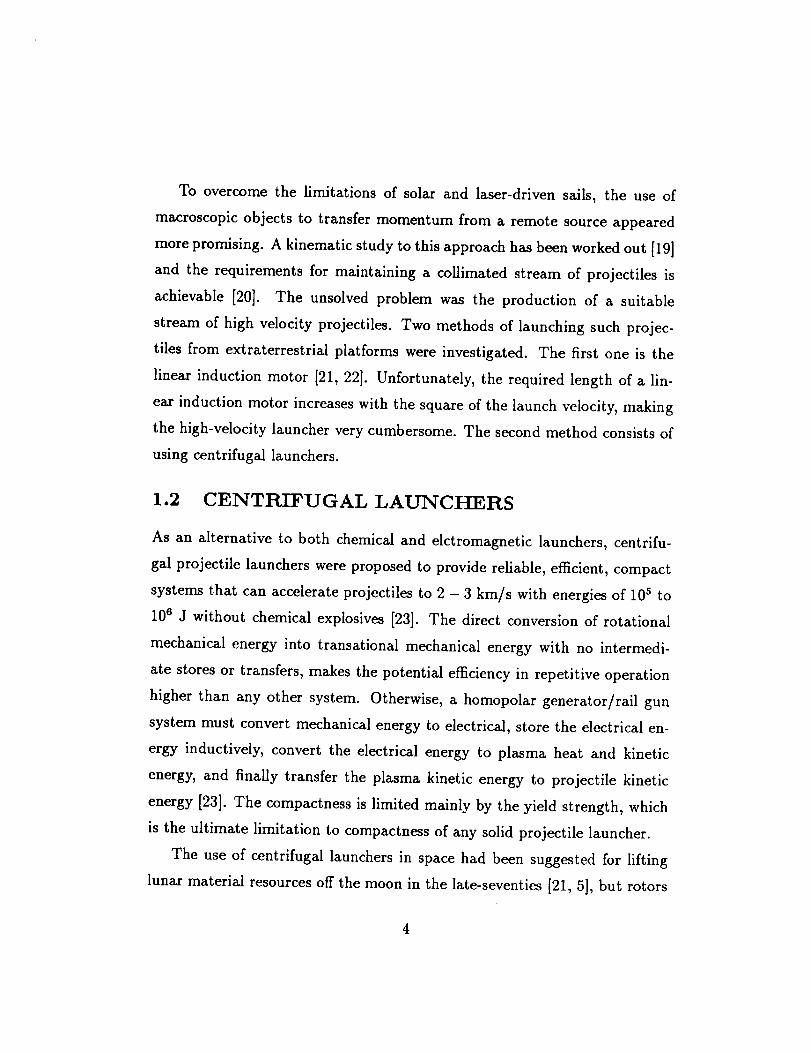
The basic idea starts with an existing centrifugal launcher [27] as illustrated

in Figure - 1 [24]. The mass driver is anchored on a large body and used

4

Figure- 1. Centrifugal launcher.

fi

to throw small masses towards a curved track or guide tube on the payload.

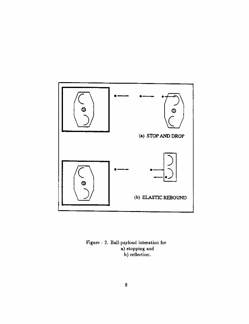
Momentum may be transferred by stopping these masses at the payload, or

more efficiently, by reflecting them back to the launcher [24]. These two

options are summarized in Figure - 2 [24].

To increase the velocity of the projectiles incident on the payload, a cen-

trifugal relay is inserted between the launcher and the payload as illustrated

in Figure - 3 [24]. The requirements on this relay are: its rotational energy

must be maintained so that it accelerates incoming projectiles to a higher

speed when passing them on to the payload; and it must be continuously

accelerated so that its velocity is intermediate between the first launcher and

the payload. This method can be extended by inserting two or more centrifu-

gal relays between the primary launcher and the payload [18]. This makes

this recently discovered method using centrifugal relays for the acceleration

of spaceborne payload to high velocity at high thrust, very attractive. It

has unique advantages over chemical rockets (low velocity - high thrust),

and other advanced methods such as plasma thrusters and solar sails (high

velocity - low thrust) [18].

1.4 OBJECTIVE

The purpose of this work is to explore the use of centrifugal relays for space-

craft propulsion in sufficient detail to assess the potential of this method for

orbit transfers requiring large velocity increments (Av's up to 10 kin/s), and

for the capture into Earth orbit of suborbital payloads. The investigation of

this potentially viable novel spaceborne propulsion concept is a joint project

between the Aeronautical and Astronautical Engineering department, and

the Nuclear Engineering department at the University of Illinois. This new

initiative in advanced propulsion systems is funded by NASA.

lu

(a) STOP AND DROP

Q ,,,,,,,,,,,-,-GD

(b) ELASTIC REBOUND

Figure - 2. Ball-payload interation for

a) stopping and

b) reflection.

8

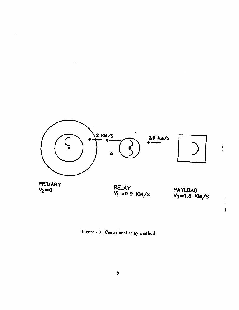
/PRIMARY

V2-o RELAYv_=0.9 Ku/s

Figure - 3. Centrifugal relay method.

9

1.5 DEFINITION OF THE PROBLEM

For the purpose of this thesis, the goal is to assess the potential of centrifugal

relays for a specific type of mission. The research can be divided into four

areas: kinematics, mechanical design, guidance, and systems. We propose to

investigate two aspects of this project and identify all the requirements for

the kinematics and the guidance system. We will then identify the concepts

of the solutions to each problem and we will define the components of each

part.

We will start in Chapter 2 by giving an overview of the launch system as

a whole, followed by a description of the kinematics involved to understand

how momentum is transferred. We will also discuss design considerations for

the rotors. We will then give in Chapter 3 a detailed description of the launch

of one ball. Then, we will add to it the catching part in Chapter 4. We will

also consider in this chapter the trajectory of the ball on the catching rotor

and investigate a delay circuit that will insure that the ball flies off this rotor

in the desired direction (which is, in this case, back to the launcher). After

this one ball, one launcher, and one relay (payload in this case) problem is

solved, we can consider the case of launching two or more balls. Then we

can study the problem of additional tracks on the relay. The purpose would

be to launch balls in the opposite direction and insure conservation of the

angular velocity of the rotor. This generalization process of launching n balls

is described in Chapter 5. We also develop in this chapter a program that

keeps track of the position of the relay as the balls are launched. It compiles

all the data necessary for the visualization of the process, such as the time at

which a ball is released near the center of the primary launcher, the time at

which it exits the launcher, the time at which it is caught, sent back to the

I0

launcher,and at what speedthe relay is moving. Finally, this rotor is to be

consideredasa launcherandthe sequencerepeatsitself. The final stepwould

be to write a generalcodethat treats arbitrary numbersof relaystaking into

account the externally imposedgravitational potential appropriate to the

mission type, but this is not in the scopeof this thesis. We are limiting

ourselvesto the completestudy of a one relay case. For guidance purposes,

we will be considering guide barrels as a first step in velocity trimming.

Electromagnetic focussing has been identified as the aiming mechanism. We

will be giving in Chapter 6 a detailed description of the tracking mechanism

(interrupt of optical beams) and the switching circuitry for the deflection coils

and all the electronics involved in the guidance system. The final step would

be to consider the system as a whole for optimization of mission profiles. One

could study the Mars mission. One could estimate the performance and the

cost of such system, and this last part is again suggested as a continuation to

this work and not part of it. We will be giving in Chapter 7 our concluding

remarks. We will summarize the results and discuss future work that we

suggest necessary before the completion of this project as a whole.

11

Chapter

KINEMATICS AND DYNAMICS OF THE

CENTRIFUGAL RELAY DESIGN

Understanding the kinematics of the centrifugal relay system is of great

importance to this project. Before we start our kinematic study, we will give

a brief overview of the whole launch system in order for the reader to get

a clear picture of the concept. We will also discuss design considerations

for the centrifugal launchers and come up with a conceptual design for the

rotors.

2.1 OVERVIEW

The overall launch system is outlined in Figure - 4 [24]. For the first step of

the launch process, a large flywheel is geared to a small primary centrifugal

launcher. The power source could be nuclear, bioconversion, or physical

conversion of solar energy [19]. Ferromagnetic ball bearings are released near

the axis onto a curved track, and exit into a guide barrel. The spherical shape

of the projectiles would minimize the influence of solar winds according to a

study by Brian Von Herzen [28], although we are not concerned in this thesis

12

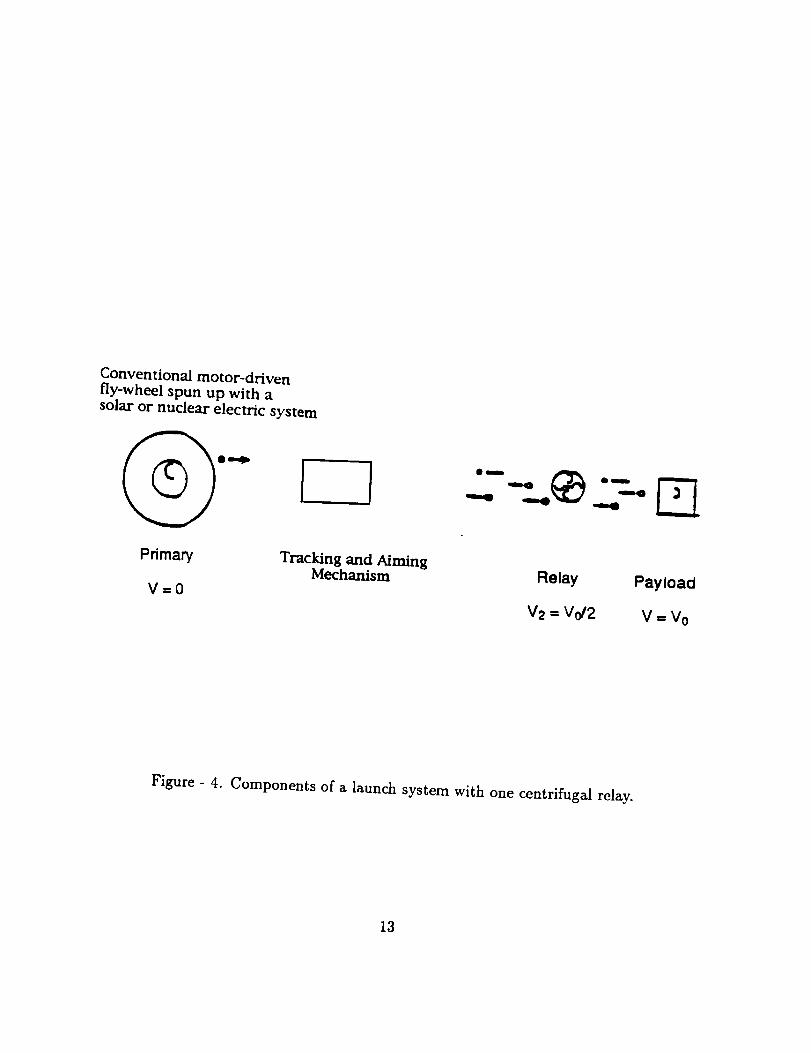
Conventional motor-drivenfly-wheel spun up with asolar or nuclear electric system

! I -"-

Primary Tracking and AimingMechanism Relay Payloacl

V = 0 V2 = Vo/2 V = Vo

Figure - 4. Components of a launch system with one centrifugal relay.

13

with the external perturbations from gravitational fields and solar winds.

For position and timing measurements,eachball interrupts at least two sets

of horizontal and vertical laser beamsdirected upon fine-scalephotodiode

arrays. For aiming, setsof top/bottom and left/right coil pairs areenergized

to impart small lateral velocity increments.Solenoidalcoils surrounding the

flight path are used to exactly time the arrival of eachball at a target rotor

0.1-10 km downstream.

The stream of balls so launchedfirst encountersa spinning relay rotor.

In a spacebornesystem, deflector shields would protect the relay against

razemisaimedballs. The rotating balls land on a guide track with velocities

matched to the track velocity sothat they roll up the track. Presentplans

call for the relay rotors to bemadeof non-ferromagneticcompositematerials.

Coils imbeddednear the rotor axisslow downthe motion sothat, whena ball

rolls backdownthe track, it leavesgoingalmostexactly forward or backward.

Forward-goingballs go on to impel the next relay or the payload assembly;

backward-goingballs arecollectedat the primary launcher. Additional tracks

on each rotor assemblyare used to processballs which land near axis to

maintain nearly constantrotational energyand/or arebeingpassedbackward

for eventual collection and reuse.

For a detailed description of centrifugal relays for spacecraftpropulsion,

the reader may refer to "Centrifugal Relaysfor SpacecraftPropulsion" by

Clifford Singer and Richard Singer [24].

For the purposeof this thesis,wewill beconsideringjust onerelay and the

balls areonly goingbackwardto the primary launcher. Themethod is general

and the results can be generalizedeasily for forward going balls impelling

other relays or the payload. Before doing this, however, it is desirable to

treat the one relay casein all details as completely as possible. We will

14

start here by describing the kinematics involved in this project and show

how the centrifugal launcherscan be usedas energyand momentum source

for spacebornepropulsionsystems.

2.2 KINEMATICS

The purpose of these kinematics calculations is the determination of momen-

tum transfer. We will start by studying the case of a one ball launch and see

how that ball transfers momentum to the payload. We will then generalize

the results and write a recursive formula that gives the momentum gained by

the payload as a function of the number of balls launched. This study will

allow us to estimate the amount of initial stored energy required to launch a

payload.

2.2.1 Momentum Transfer after the Launch of the First Ball

The approach here is similar to the one followed by Clifford Singer and

Richard Singer [24]. The general linear momentum conservation equation

can be written for this system as:

(1)

where m is the mass of the ball and M is the mass of the rotor catching the

ball or, eventually the payload. _,, is the velocity that the ball has when it

leaves the primary launcher and ffo,,t is its velocity after it impacts the relay

or payload, and rolls back off the track heading back toward the primary

launcher. Vii,_ is the relay/payload velocity before the launch of this first ball,

and P'o,,t is its velocity after this first launch is completed.

The energy conservation equation can be expressed in terms of the rota-

15

tional energy E,.ot, gained by the relay as:

1 2 1MVi_ ] 1 2 1 2

total initial l_inetic energy total final kinetic energy

or,

2E,.ot = m(v_. - 2 M(V_ - _vo.,)+ v;.,). (3)

Let us denote by Ag the decrease in ball velocity,

Aft= _7_. - fro.,. (4)

Then, the momentum lost by the ball is mAff. It corresponds to the momen-

tum gained by the rotor M(Vo,,- G,,). So, the momentum transfer can be

written as:

M(_'o.t - _,,) = rnAK (5)

Equation (3) can be rewritten as:

2E,.o, = m(_,,_ - G,_t)(ff,_, + G.t) + M(_,., - ¢o.t)(G,, + _'o.t),

and, using Equations (4, 5), it becomes:

2E,.ot = mA$(_. + G.t) - rnA$(_'i,, + _'o.,).

Now, we can still substitute (fi'_. - Aft') for _7o.t from Equation (4) and,

(G. + _Ag) for Vo.t from Equation (5) in the equation above and get:

In the case of the payload, there is no rotational energy transfer

(E,.ot = 0). Equation (6)can then be written as:

2(_,, - G,,) = Ag(1 + ---_),

16

or, using the definition of Aft:

2(_

1+"

and finally,

+ _.(-1 + gl_o.,= --" M, (7)

1+"

We can also determine the increase in payload velocity as:

17out_Q,_= m ... m _,_Av =

Substituting for ffo,,t from Equation (7), the increase in payload velocity be-

comes:

_o.,- _,. = m 2(_,. - ¢,.) (8)M 1+ '_

Now, if we go back to the case of a relay, the rotational energy is generally not

zero. It can be obtained from Equation (6) provided Ag has been determined.

In the next chapter, we will determine the

we analyze its interaction with the relay

have to mention here that our study will

final velocity of the ball, go,,t after

using Lagrangian mechanics. We

assume an infinite mass rotor. In

practice, the rotor is about 10 kg and the ball is just a few grams. The ratio

m/M is of order 10 -4, which justifies our assumption of infinite mass relay.

If we were to take into account the finite mass of the relay, the Lagrangian of

the system would be more complicated and the angular velocity of the relay

would not be constant but would be an extra unknown to be determined.

This would complicate the analysis. We will thus simplify the Lagrangian

and study the interactions of the ball with an infinite mass rotor, keeping in

mind that we have an error of the order of (re�M) 2 stepwise according to

Equation (8), where the increase in velocity of the relay would be:

17

,._ rn _. (1-- .

Knowing that m/M ,.-, 10 -4, we believe this is a quite good approximation

and we will definitely consider in the next chapter an infinite mass rotor. We

can also estimate at this point the cumulative error after the launch is com-

pleted. We will be throwing balls on this rotor to increase its velocity until it

becomes comparable to the velocity of the incoming balls, _7i,. According to

Equation (8) again, the total number of these increments would be M/2rn.

So, the total error can now be determined by multiplying the total number

of increments by the stepwise error. The cumulative error is estimated to be

of the order of m/2M.

In the case of an infinite rotor mass, the rotational energy gained by the

relay is zero, making the cases of relay and payload similar. Furthermore, if

we start for this first ball launch with an initial zero velocity for the relay

(V/, = 0), we get from Equation (7):

and from Equation (8):

_t m ..

which represents the limiting case of an elastic collision where the ball trans-

fers twice its momentum to the relay. Now, we can determine the actual

rotational energy if we consider a step by step analysis and write the angular

momentum conservation equation. The angular momentum lost by the ball

will be gained by the rotor. Knowing if,., and ffo,,t from the Lagrangian anal-

ysis, we can write the angular momentum/_ before and after the interaction

18

respectively as:

and

f_ = _,, X rn_,

where _,_ is the position vector when the ball impacts the track on entry, and

Four its position at the exit of the track when traveling back to the primary

launcher. Then, the decrease in the ball angular momentum, f_i,, - f-,o,,t will

correspond to the increase in angular momentum of the relay, A[,,oto,. And

finally, if we know the moment of inertia of the rotor, Z, oto,. we will determine

the increase in its angular velocity Aw from:

A/,,o_o, = -Loto,AS.

2.2.2 Momentum Transfer after the Launch of n Balls

Let us now consider a sequence of such interactions and derive a recursive for-

mula giving the increase in relay/payload velocity as a function of the number

of balls launched. The relay/payload initial velocity, before the launch of the

first ball, is V_,,. After the impact of the first ball, the velocity becomes:

as shown in Equation (8). We can now write the final velocity of the re-

lay/payload after the second ball is launched:

m(_,,-_) + .-, ('7,,,- V,,. +2_",+_ '0 )Vi" + 2M 1+_ 2M 1+_ '

or,

19

We also derived the result for the case of three bails launched (n = 3):

.... _-_ •[1+

We went on and wrote the velocity resulting after 4 balls have been launched,

and also after 5 balls were launched. We then expressed the general formula

giving the final velocity of the relay/payload after n balls are launched as:

p=t p [1 + _](9)

We then wrote a little program (cf. APPENDIX), that uses the expres-

sion derived above and computes the velocity of the relay after n balls are

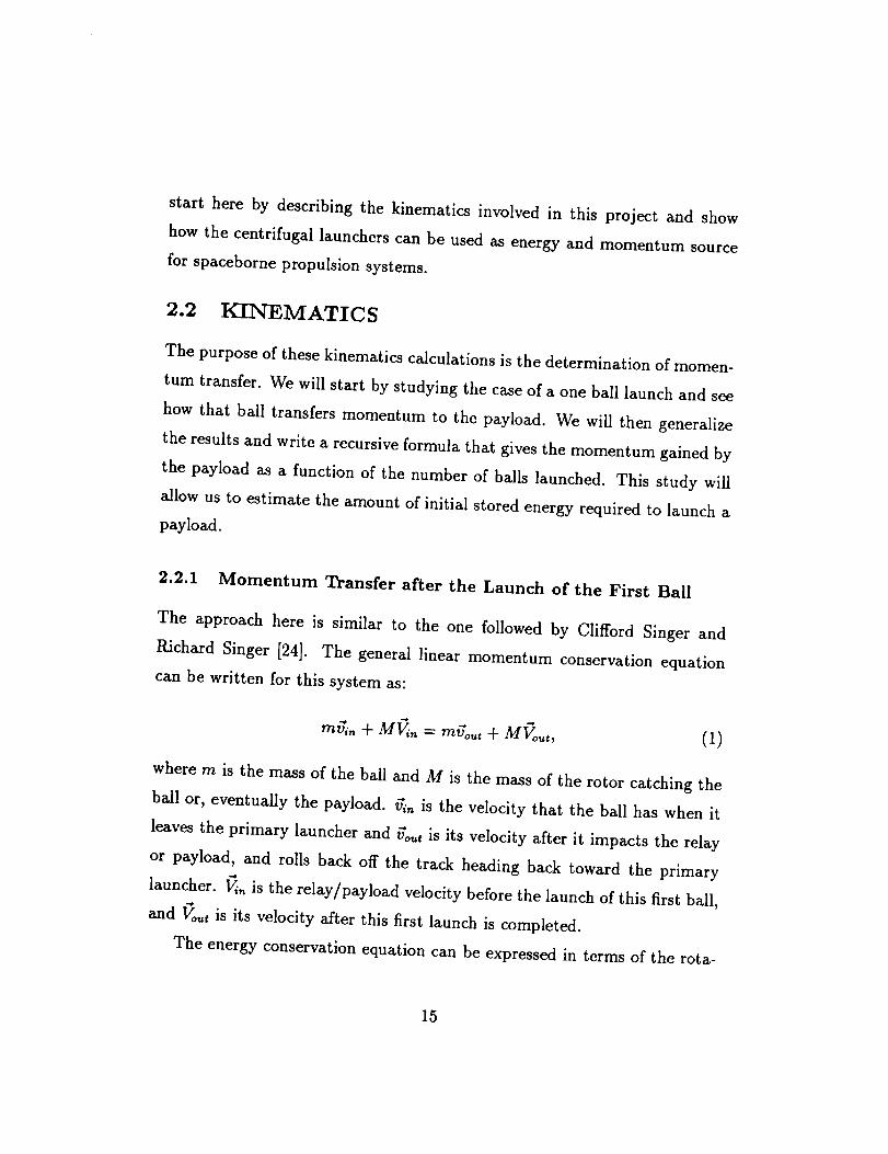
launched. We plotted in Figure - 5 the generated data to show how tPo,,t

varies with n. We can see that the velocity of the relay increases almost

linearly with the number of balls launched, but then, as the relay is going

faster and faster, the effect of one ball becomes less and less important. Very

little momentum is transferred when the rotor is moving at speeds similar to

the speed of the incoming balls, until it reaches the speed of the balls and

they will not be able to catch up with it. In the practical case considered

here, some 8000 balls would be needed to reach a velocity v,._t,,_ = 1698 m/s.

Only the first 10% of the total number of balls needed to reach this limiting

case of a relay moving, practically as fast as the balls, will provide half of

the final rotor speed while the remaining 90% of the balls will provide the

remaing half of the total velocity increments. This suggests that one should

accelerate the relay until it reaches about half the velocity of the incoming

2O

1.33

Velay

(kin/s)

0.67

2

0

0.0 1 0 °

' ' ' I ' ' , I ' ' ' I _ '

, , I , , ,. I , i , ! i ,

2.0 103 4.0 103 6.0 103 8.0 1 03

Number of balls

Figure - 5. Velocity of the relay versus the number of balls launched.

21

balls as further acceleration would not be cost effective since the balls are

not as efficient in terms of momentum transfer.

2.3 DESIGN CONS/DE;RATIONS :FOR TI-]_ C_',N-

TRIFUGAL RELAYS

One major design consideration is the fact that the relay must process a

large number of balls quickly and efficiently. The rotor is a disk or a cylinder

spinning at high angular velocity with guide tracks to process the balls in

the necessary direction. The balls are either caught near the axis of the rotor

and launched forward or caught nearer the tip of the rotor, slowed to a stop

at the axis and then propelled forward or backward using another track. The

objective of the first type of processing is to increase the velocity of the bails.

The second type of processing increases the angular and linear momentum

of the relay. For the determination of the exit velocity and the forces of

constraint on the ball, a track shape needs to be chosen. If the ball starts at

the center of the rotor and is launched tangentially, it leaves with twice the

tip speed of the rotor, where the maximum tip speed depends on material

properties of the rotor [23]. The shape analyzed here is the logarithmic spiral.

The objective is to develop a method that can be used to analyze different

shapes quickly and easily.

Original studies of the kinematics of ball/rotor interaction idealized the

relatively small bails as point masses [24]. Then an equation of motion treat-

ing the pellet as a ball of finite radius was derived [29]. One constraint to

be satisfied is that the balls must not bounce nor slide during the catching

process to insure a maximum exchange of momentum between the ball and

the rotor. This constraint is satisfied if the velocity vectors of the point of

impact on the ball and the blade are equal. We have started detailed kine-

22

matic studiesby assumingthat the velocity vector at the edgeof a ball rolled

off a previous rotor must match the velocity vector of the contact point on

the next rotor it encounters. This condition is met by slightly adjusting the

aiming and timing so each ball launched encounters the next rotor at the

correct distance from this rotor's axis. This removes a degree of freedom

which complicated the analysis made in the paper "Centrifugal Relays for

Spacecraft Propulsion" [24]. This should considerably simplify the next step

in the kinematic analysis-writing a computer program which follows the tra-

jectories of all objects in the system in the presence of a gravitational field.

To obtain an even more complete description of ball/rotor interactions,

AUTOLEV program may be used. This program, by Schaechter and Levin-

son [30], automatically generates FORTRAN coding for complete solution for

rigid body kinematics of finite mass balls interacting with a free-flying rotor

in a gravitational field. While including the effects of finite ball/rotor mass

ratio is not expected to be important for the kinematics of the overall mission

performance, it will determine the exact amount of magnetic drag needed to

hold the balls near the rotor axis long enough that they will roll back off

at the right time. The same method can also be used to examine various

schemes for emplacing and activating these coils. To date, the AUTOLEV

program has been successfully used for balls landing with properly matched

velocities, rolling up towards the axis of a rotating relay, and rolling back off

the track for relaunch [31]. The program is designed so that investigation

of additional effects like small velocity mismatches at catch, finite ball/rotor

mass ratios, and gravitational fields are straightforwardly accomodated by

changes in the program input.

23

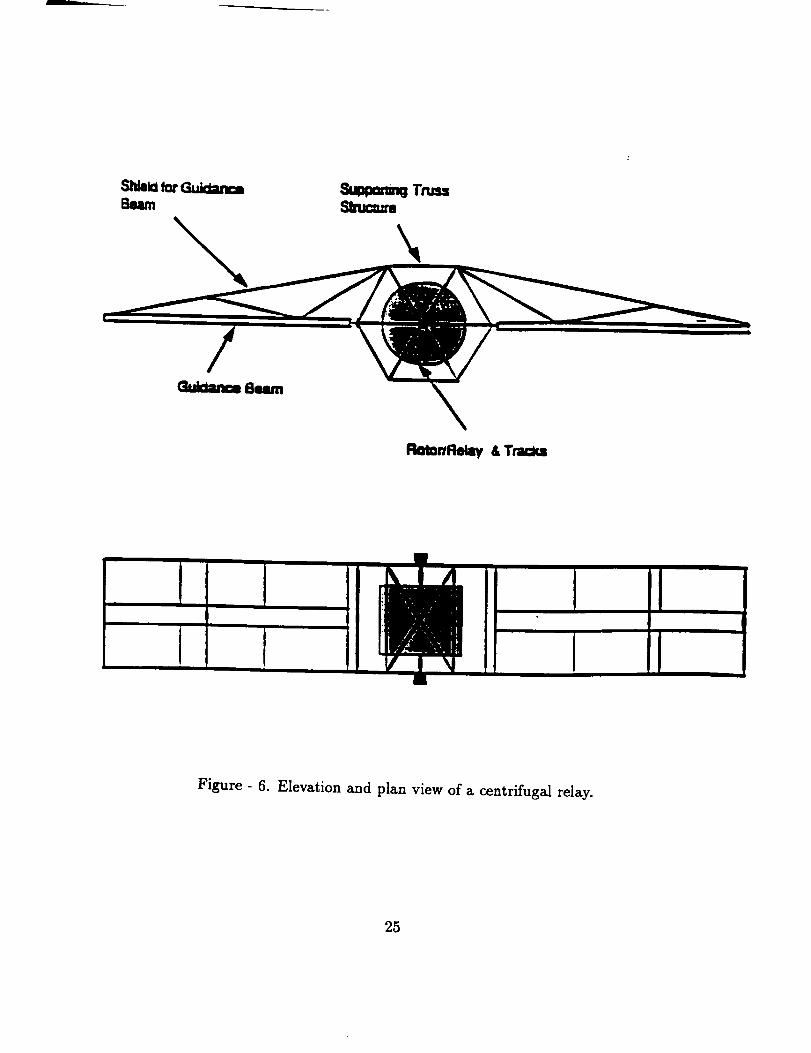
2.4 CONCEPTUAL DESIGN OF THE RELAYS

The first task in designing the centrifugal relays is coming up with a con-

ceptual idea. The rotor has to have guide tracks for the pellets. It should

spin at very high angular velocity processing balls in both directions. The

rotor should include guidance tubes in the path of the incoming pellets for

position control. A protection shield has to be placed in front of the guide

tubes and rotor to prevent errant bails from impacting these systems. A

supporting truss structure is needed to mate the rotor, the guidance tubes

and the protection shield. To minimize the total system mass, the size and

the mass of the whole relay may need to be kept small. This conceptual

design can be summarized schematically as illustrated in Figure - 6 [32].

2.5 DESIGN CONSIDERATIONS FOR THE RO-

TOR

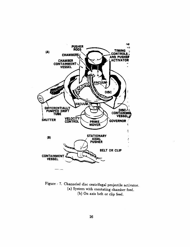
The basic concept of a centrifugal projectile accelerator is that a projectile

can be accelerated centrifugally by either being constained to move along a

channel in a rotating disk or arbor, or by being released from the edge [23].

Figure - 7 illustrates such launcher [23].

The rotor is a disk or a cylinder spinning at high angular velocity with

guide tracks to process the balls in the necessary direction. The "forward"

or "backward" launching depends on the objective of the launch. It could be

increasing the velocity of the ball, or the angular and linear momentum of

the relay. The idea in this design is to have one rotor accomplish one task.

For example one rotor would catch the balls near the tip and slow them to

a stop at its axis increasing the rotational and transitional velocity of the

relay. The balls would be collected at the axis of this rotor and then fed to

24

RmortRetlly & 1"_

Figure - 6. Elevation and plan view of a centrifugal relay.

25

(A)

.,_.PUSHER :_.

RODS TIMING ._CHAMBERS,

AND PUSHE]WCHAMBER ACTIVATOR

CONVESSEL

VELOCITYCONTROL

CONTAINMavUSZL.

GOVERNOR .';

(B) STATIONARYAXIAL

BELT OR CLIPCONTAINMENT 6".=..\ .'.._._._-_. _1__

VESSEL , __

i

.t

Figure - 7. Channeled disc centrifugalprojectileactivator.

(a) System with corotating chamber feed.

(b) On axis belt or clipfeed.

26

another disk to be propelled in the necessary direction (forward or backward).

A display of this concept is given in Figure- 8 [32]. The disks are all rotating

at the same rate. The balls are fed through the shafts to the correct track.

In practice, instead of having several disks, we will just use a multiple track

rotor.

Another point discussed here is whether the rotor should be a cylinder

with a track bored through it or a rotating disk with a surface track. The

latter case may seem more interesting for reasons of machining and catching

incoming balls. It is easier to catch the ball on a surface track then in a small

hole. But the track bored through a cylinder may be more practical for the

transfer of the ball from one track to the other at the center. Conceptually,

the best design would be a combination of these two alternatives. We would

have a surface track starting at the edge of the rotor and continuing into a

path bored through the rotor. The track will end at the axis of the cylinder.

The second track will start from the center at a lower level and emmerge to

the surface toward the tip of the rotor.

Typical materials of interest for use in a pellet launcher are given in

Table - 1 [33], where V_ represents the critical velocity, p is the density and

a the yield strength of the rotor material. To build a launcher that ejects

pellets with velocities less than V_, we can just use a tube of uniform cross

section. Above V_, the pellet launcher must be tapered for part of its length,

increasing in thickness toward the axis [33].

The tube may be subject to considerable wear due to friction and abrasion

from the pellets, and should be designed for easy maintenance. This could be

accomplished by providing the tube with a removable liner, and by designing

other high - wear parts for easy removal and replacement [33].

The U. S. Department of Energy has designated Lawrence Livermore

27

b_t canbe_ed _l'et_,'own back

Figure - 8. Multiple track relay concept.

28

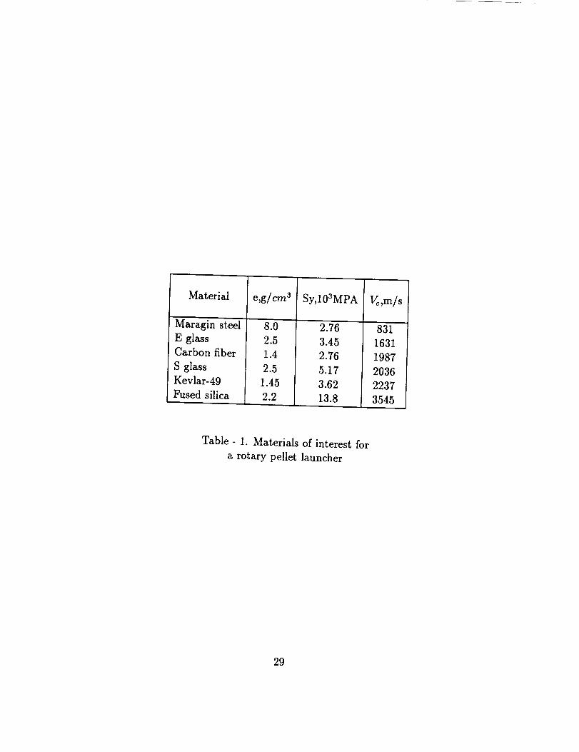
Material

Maragin steel

E glass

Carbon fiber

S glass

Kevlar-49

Fused silica

e,g/ cm 3

8.0

2.5

1.4

2.5

1.45

2.2

Sy,103MPA

2.76

3.45

2.76

5.17

3.62

13.8

Yc_m/s

831

1631

1987

2036

2237

3545

Table - 1. Materials of interest for

a rotary pellet launcher

29

National Laboratory the leadlaboratory in its flywheel rotor and technology

developmentprogram. Although the objective of that program wasstoring

energy,the rotors that were developedcan be modified to launch projec-

tiles [23]. One of the near-term objectivesof this program is to developan

efficient,economical,and practical compositeflywheel. State-of-the-art com-

posite rotors developedin the program [34] have maximum tip speeds< 1

km/s. Their radii are typically 10 - 20cm, and massesarea few kilograms.

Thesecentrifugal launchersaresummarizedin Table - 2 [23].

For the determination of the exit velocity and the forces of constraint

on the ball, a track shapeneedsto be chosen. The launch should be such

that the exit velocity is approximately twice the tip speedof the rotor. The

maximum tip speed,Vc is proportional to (a/p) '/_ [231.

The shape considered is the logarithmic spiral. An illustration of the

track shape is given in Figure - 9. The method developed should be general

and could be applied to analyze different shapes quickly and easily. This is

the subject of the next chapter, a detailed analysis of the launching process.

3O

Rotor State-of- Near-Term-DOE Demothe-Art Objective

0.24 0.32 0.57Maximum energydensity (MJ/kg)Maximum rotationalenergy (MJ)Mass (kg)

Radius (cm)

Maximum frequency

(rpm)

Maximum tip

speed (km/s)

0.62

2.6

20.3

49,000

1.04

3.6

11.2

30.5

35,400

1.13

3.4

6

120

12,000

1.5

Projectiie State-of- Near-Term:DOE Demo

the-Art Objective

Mass (g)

Maximum velocity

(km/s)

Maximum energy

(MJ)

26

1.04

0.014

112

1.13

0.072

60

3

0.27

Table - 2. Rotors and launching capabilities

31

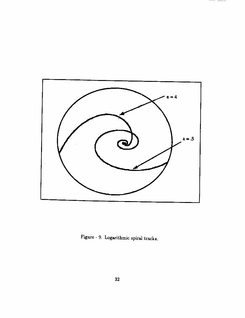
a = .5

Figure - 9. Loga_ithraic spiral tracks.

32

Chapter 3

ANALYSIS OF THE LAUNCHING

PROCESS

Lagrange equations with multipliers are used to analyze the launch pro-

cess. The track shape is represented as a constraint equation between the

radial and angular positions. A second constraint equation represents the

fact that the ball is restricted to roll on the track. We wish to avoid skidding

because frictional losses would make the system non-conservative.

The velocity of the center of mass of the ball along the track is:

v2 = ÷2 4-r2(_2, (10)

and

O(t) = Oo +wt + C(t), (11)

where r is the radial displacement of the ball, w the rotation speed of the

rotor, _ the angle that defines the position of the ball along the track, and

0o any initial angle that might be present as illustrated in Figure - 10. If we

let m be the mass of the ball, then the kinetic energy is:

1 2

33

r1

! Track: r = ro e a_

a=l

0< _<2.3 rad

r o

Figure - 10. Track on primary launcher.

34

where 2- is the moment of inertia of the ball defined as

Z = _me 2, (13)

being the radius of the balland & the angular velocityof the ball around

its center of mass. These quantities are all defined in Figure - 11.

The Lagrangian is:

L=T-V=T

since there is no potential energy.

The constraints equations are:

fl = r0e_c(t)- r(t)= O,

(14)

(15)

and

f2 = e,_(t)- s(t) = o, (16)

where s, the track shape length defined in Figure - 11, is related to r as

follows:

ds 2 = dr 2 + r2d_ 2, (17)

or,

T_ = 1+ r_ _ (18)

Now, from Equation (15), we can write:

(=lln ra r 0

d E 1

dr ar

Then,

=l+--a2 _

(19)

(20)

(21)

35

r(t)

a (t)

S (track distance)

_;(t)

Center of relayI (radius)

m m

Figure - 11. Rolling of the ball on the track.

36

or_

Integrating this equation and using the initial condition s = 0 when r = ro

to determine the constant of integration, we can write s(t) as a function of

_(t):

and ]'2 becomes:

f2=&r(t)-(_(r(t)-ro)=O.

The equations of motion are:

(24)

and

d(OL I OL Of 1 Of 2-87 - 0-7= A, --_-+ _2--_ ,\/

d[0L 0L 0f,

(25)

(26)

(27)

Dividing Equation (25) by m gives:

_r(w+_)_+A'__+__V_+ 1m _-

Equation (26) can be written as:

A,_ + 2_÷(_+ _) - a_- = 0.

m

=0. (2s)

(29)

37

Dividing Equation (27) by 2- gives:

A2

a - Te = o. (30)

From Equation (30) combined with Equations (16, 23) differentiated twice

with respect to time, we get:

_2= 74 = ?_= _.

Solving for A1 from Equation (29) we get:

__,= 2_÷ + 2÷_+ _. (32)7"t2 a a a

Now, substituting for ,_1 from above and )_2 from Equation (31), and using

the following set of equations derived from Equation (10)

_= --,÷ (33)ar

and

Equation (28) becomes:

_= 1 r/: - ÷2a r2 , (34)

or simply,

where

[1 _ _] [_ _]÷2 -a-_r + + ÷ --- + - rw2a2 r a_r, = 0, (35)a

- K_r = 0, (36)

K s _-_j2

(1 + _)(1 + if)'(37)

38

and

We can also write K s as:

2"

m_2"

5_ 2K__ (3s)

taking into account the fact that the projectiles have a spherical shape, which

means:2

J __ _.

5

The corresponding solution to the governing equation is:

r(t) = AcoshK(t -to) + BsinhK(t - to). (39)

Differentiating this equation, we can write:

÷(t) = AK sinh K(t - to) + BK cosh K(t - to). (40)

Now, at t = to, when the ball is released near the center, we have:

r(to) = to,

and

Consequently,

and

,:(to)= o.

A = to,

B-O.

The trajectory of the ball on the track is then given by:

,'(t) = ro cosh K(t - to). (41)

39

One quantity of interest is the exit velocity. It can now be determined,

and we can study its behavior as a function of the designparameterssuch

asthe track shapeconstant a.

3.1 EXIT VELOCITY

The position of the ball on the rotating track with respect to a fixed frame,

with 0o = 0, is given at all times by:

r-'(t) = ( r°e_¢tO c°s(wt + _(t)) ) . (42)roe <_`_ sin(wt + ((t))

We can get the velocity vector by differentiating the position vector above,

roaCe"¢(0 cos(wt + ¢(t)) - ro(w + ¢)e"_(0 sin(wt + ¢(t)) i. (43)roaCe "¢(0 sin(wt + ((t)) + ro(w + ¢)e _¢('} cos(wt + ¢(t)) )

Then,

Using Equation (33), v 2 can be written as:

ff+w +a 2

Now, from Equation (41) we get:

(44)

5]. (45)

÷ = KrosinhK(t - to). (46)

This can be combined with Equation (41) to express a relationship between

r and ÷,

÷= K ro (47)

4O

Substituting for ÷ from Equation (47) and K from Equation (38) in Equa-

tion (45) we get:

And finally, we can write the exit velocity v,xit as:

(48)

l_e_cit "- ?)_ip 1+7 _j/+ -, (49)

where vtiv is equal to wrt.

Also from the geometry, as outlined on Figure - 12, we can write:

d_ _/_¢tan-y = d--x = dx/d¢'

where tan 3' is the slope of the tangent to the track at the exit, and x and y

are given by:

and

We can also write tan 7 as:

tan _ =

z = e< cos(¢ + wt),

y = e"¢ sin(¢ + wt).

a sin(¢ + wt) + cos(¢ + wt)

a cos(¢ + wt) - sin(¢ + wt)"

Now, let us express _ in terms of 7. We can write, after inspecting Figure - 12:

7r

¢ +,,,t =/_+-y- _,

41

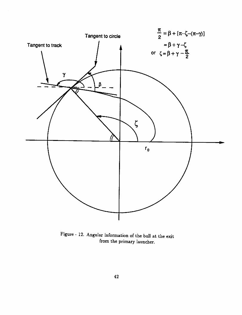
Tangent to track

Tangent to circle

or _=13+_'-_"

r o

Figure - 12. Angular information of the ball at the exit

from the primary launcher.

42

where 8 is the angle between the tangent to the rotor rim and the tangent

to the track at the exit. Using this relationship between the angles, tan-),

becomes:

-a cos(_/+ 3') + sin(fl + 7) sin 3'

tan7 = asin(8 + 3') + cos(8 + 3') = cos----_"

This equation can be rewritten as:

-a cos(8 + 3')cos3'+ sin(8 + 3')cos3'= a sin(8 + 3')sin3'+ cos(8 + 3')sin 3',

or simply,

-a cos fi = - sin 8.

Thus, the main result of this geometrical derivation is:

tan fl = a

or_1

cos8 - 4"f + ,_2

If the ball leaves from the center (to = 0) tangentially (8 = 0) Equa-

tion (49) becomes:

Ve_:it = 1.84vtip,

and we can see that the ball leaves with almost twice the tip speed of the

launcher. Felber [23] stated that the ball leaves with twice the tip speed in

the same conditions of launch. But in his case, the ball was considered as a

point mass with zero inertia (e --, 0), which means that all the energy gained

by the ball is used for the translational displacement of the ball, whereas

in our case, some of the energy is used to spin the ball around its center

of mass. So, the resulting translational velocity is less than in the case of

43

Felber's calculations, and in general, the exit velocity does depend on the

inertia of the projectile. We can actually find his result from our general

expression just by setting ff - 0 (no inertia) in Equation (37) which gives:

K 2 __

1+ 3"

Then, substituting for ÷ from Equation (47) and K from above in Equa-

tion (45), we find:

v,_.i,=vtip 2-(r°_2+2 1- ro _ 1

or, as a function of the angle fl at launch,

which is what Felber [23] published. In this particular case, we can see that

when the ball leaves from the center (r0 _ 0) tangentially (fl = 0), it leaves

with twice the tip speed (v,,it = 2vtip).

The dependency of the exit velocity on the track shape constant a is

illustrated in Figure - 13.

Another important point about this launch process analysis is the deter-

mination of the time delay needed to insure that the ball is launched exacly

forward. The ball will be kept near the rotor axis while launcher is rotating

until the track is oriented in such a way that when the ball rolls off the edge

it is going exactly forward.

44

1.9

1.8

Vxit/Vti p

1.7

1.6

1.5

1.4

0 2 3 4

a (track shape constant)

5

Figure - 13. Exit velocity of the ball versus the track

shape constant.

45

3.2 TIM_ DELAY NEEDED TO INSURE LAUNCH

EXACTLY FORWARD

The position of the ball on the rotating track is given by Equation (42) and

its velocity by Equation (43). In order for the ball to go exactly forward

(horizontally), ff at the exit should be of the form:

Let tl be the time at which the ball leaves the launcher, and to the time

at which the ball is released near the center of the rotor. The origin of

time (t = 0), is taken to be at the beginning of the spinning process of the

launcher. We can determine the time it takes for the ball to roll down the

track all the way to the edge, which is (tl - to), by solving Equation (41) at

the exit (t = tl), where r(t) will be set equal to rx. Then we can get the total

launch time tl by setting Equation (43) at the exit equal to Equation (50).

Finally, the delay time to can be determined just by combining these two

results.

3.2.1 Determination of (tl - to)

At the exit, Equation (41) becomes:

(tl) = = coshZ(t - to).

This equation can be solved for (tl - to) as:

tl - to = _-_ cosh -1

(51)

(52)

46

3.2.2 Determination of tl

Equation (43) can be rewritten as:

( ÷ cos(wt + ¢) - r(w + _) sin(wt + ¢')vV

(53)

At the exit, t = tt, the two components of the velocity vector have to

satisfy the condition expressed in Equation (50). We must have vv = 0 or,

,z,sin(wt,+ _,) + r,(w + _I)cos(wh + _i) -" O, (54)

where the subscript "1" means that the quantity is taken at the exit. This

equation can also be written as:

rlr:, tan(w/, + ¢,) + r,w + r,-- = 0. (55)

arl

Then,

wt, + _1 = arctan [ 1 ]rl

a _w + kr, (56)

where ÷: can be obtained from Equation (47) and ¢1 from Equation (19)

where we replace r by ft. Finally, we can write the expression of tl as a

function of the parameters of the system:

1(tl = -- arctan03

l T'IW

a +kr- 1 In r_o)a(57)

The parameter k is adjusted so that the results are physically acceptable.

The value of tl must be greater than (tt - to) found previously. We can

check the accuracy of the results here by plugging the expression of tl above

47

into the first component of the velocity vector at the exit, VH and it should

satisfy the equation vH = v,_,.

These calculations can now be applied to the practical case we are con-

sidering and the actual values of to and tl can be determined. This will allow

us to have a good picture of the launching process.

3.3 APPLICATION

The practical case considered is as follows:

• The radius of the rotor is: rl = 0.1 m.

• The distance from the center of the rotor at which the ball starts the

acceleration process is: r0 = 0.01 m.

• The track shape constant is taken as a = 1.

• The launcher is rotating at an angular velocity w = 10000 rad/s,

which gives a tip speed of vtlp = 1 km/s and a revolution period of

T = 2r/w = 0.63 ms.

The results are as follows:

1. The ball leaves the launcher with an exit velocity v_it = 1.7 km/s.

2. The timing is such that:

• tl - to = 0.5 ms from Equation (52),

• tl = 0.9 ms from Equation (57), where k = 4,

• and to = 0.4 ms.

48

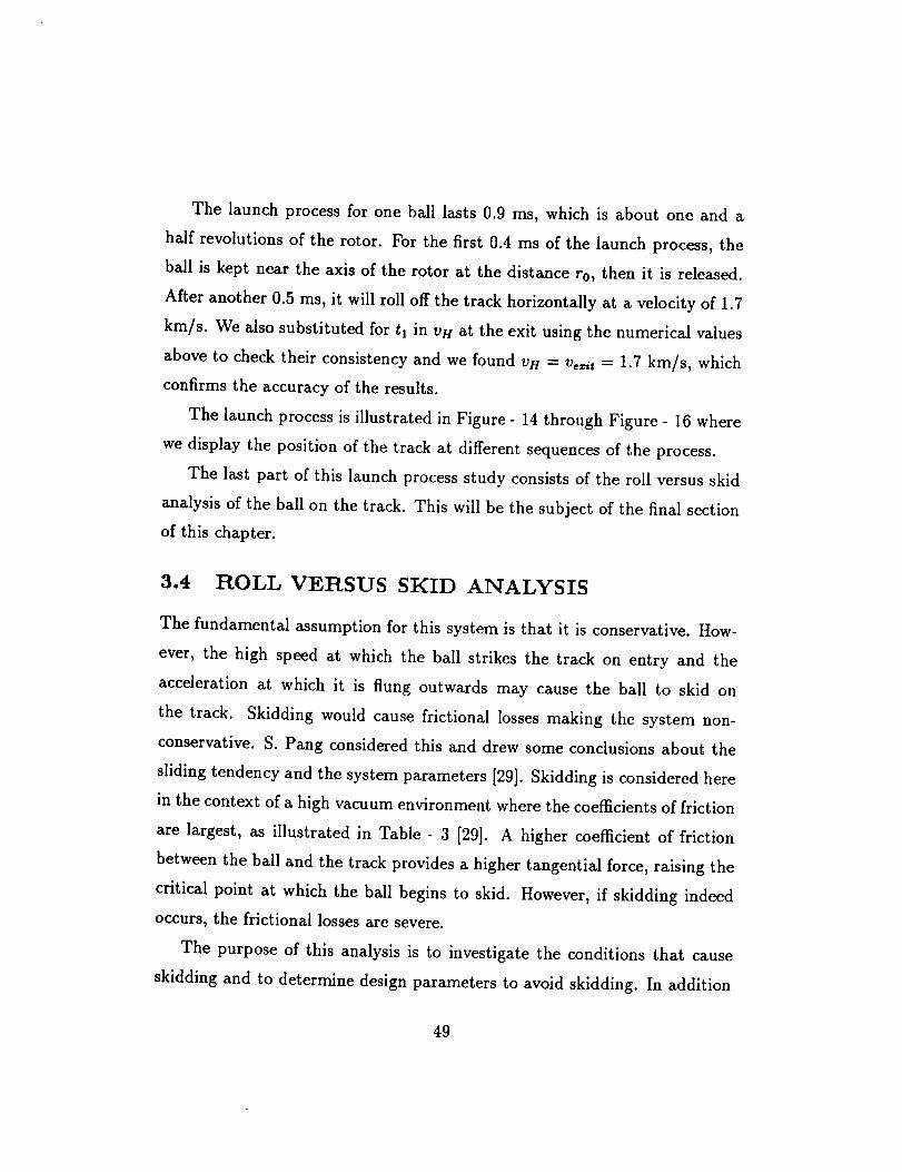
The launch processfor one ball lasts 0.9 ms, which is about one and a

half revolutions of the rotor. For the first 0.4 ms of the launch process, the

ball is kept near the axis of the rotor at the distance r0, then it is released.

After another 0.5 ms, it will roll off the track horizontally at a velocity of 1.7

km/s. We also substituted for t_ in vn at the exit using the numerical values

above to check their consistency and we found vH = v,,/t = 1.7 km/s, which

confirms the accuracy of the results.

The launch process is illustrated in Figure - 14 through Figure - 16 where

we display the position of the track at different sequences of the process.

The last part of this launch process study consists of the roll versus skid

analysis of the ball on the track. This will be the subject of the final section

of this chapter.

3.4 ROLL VERSUS SKID ANALYSIS

The fundamental assumption for this system is that it is conservative. How-

ever, the high speed at which the ball strikes the track on entry and the

acceleration at which it is flung outwards may cause the ball to skid on

the track. Skidding would cause frictional losses making the system non-

conservative. S. Pang considered this and drew some conclusions about the

sliding tendency and the system parameters [29]. Skidding is considered here

in the context of a high vacuum environment where the coefficients of friction

are largest, as illustrated in Table - 3 [29]. A higher coefficient of friction

between the ball and the track provides a higher tangential force, raising the

critical point at which the ball begins to skid. However, if skidding indeed

occurs, the frictional losses are severe.

The purpose of this analysis is to investigate the conditions that cause

skidding and to determine design parameters to avoid skidding. In addition

49

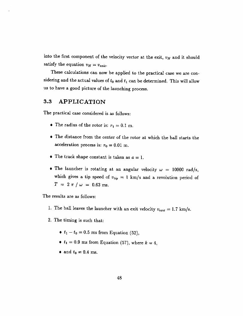
Figure - 14. Track orientation at the instant t = 0.

5O

Figure - 15. Track orientation at the instant t = to = 0.4 ms.

The ball is now released near the center of the lanucher.

51

Figure - 16. Track orientation at the instant t = tl = 0.9 ms.

The ball now rolls of the track.

52

Material Pair

P,I-AI

Be-Cu-Be-Cu

Brass-Brass

Copper-Copper

Be-Cu-Brass

Cu-Steel

Cr-Cr

Stainless Steel-

-Stailess Steel

In Air

0.78

0.58

0.32

1.04

0.38

0.55

0.85

0.51

In High Vacuum

1.57

1.10

0.71

2.00

0.9

0.96

1.30

0.93

Table - 3. Table of coefficients of friction

53

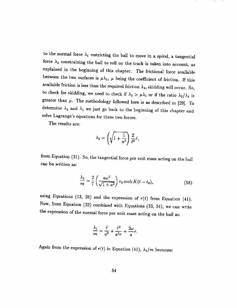
to the normal force A1restricting the ball to move in a spiral, a tangential

force X2 constraining the ball to roll on the track is taken into account, as

explained in the beginning of this chapter. The frictional force available

between the two surfaces is /_A_, /_ being the coefficient of friction. If this

available friction is less than the required friction As, skidding will occur. So,

to check for skidding, we need to check if X2 > _X1 or if the ratio )_/X1 is

greater than _t. The methodology followed here is as described in [29]. To

determine A2 and A1 we just go back to the beginning of this chapter and

solve Lagrange's equations for these two forces.

The results are:

(_ :I-..=

from Equation (31). So, the tangential force per unit mass acting on the ball

can be written as:

m = 7 k_] rocoshK(t-to), (58)

using Equations (13, 38) and the expression of r(t) from Equation (41).

Now, from Equation (32) combined with Equations (33, 34), we can write

the expression of the normal force per unit mass acting on the ball as:

,_1 /: ÷2 2w

m -- a 2 + _ + --7:"a2r a

Again from the expression of r(t) in Equation (41), X_/m becomes:

54

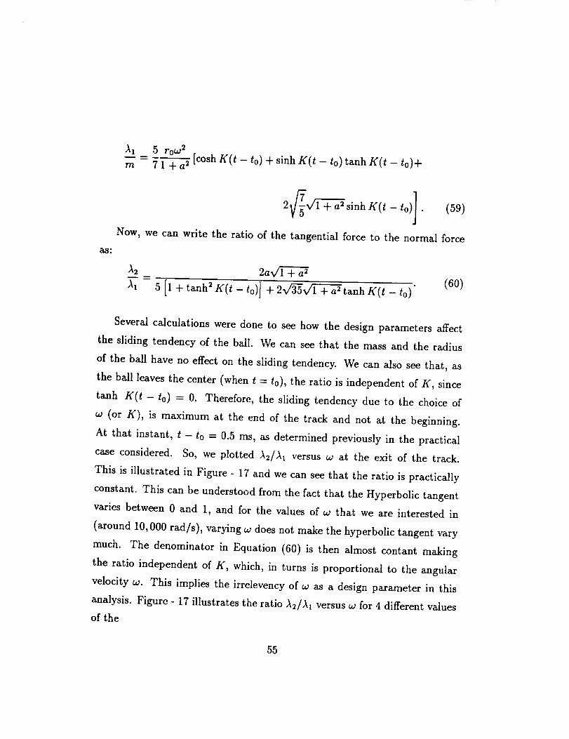
as:

A_ _ 5r°wZ [cosh K(t - to) + sinh K(t - to) tanh K(t - to)+m 71 +a 2

2V/_v/'f + a2 sinh K(t - to)] . (59)

Now, we can write the ratio of the tangential force to the normal force

A2 2avfi " + a s-- = . (60)

A, 5 [l +tanh2K(t_to)] + 2v/_V_ +a_tanhK(t-to)

Several calculations were done to see how the design parameters affect

the sliding tendency of the ball. We can see that the mass and the radius

of the ball have no effect on the sliding tendency. We can also see that, as

the ball leaves the center (when t = to), the ratio is independent of K, since

tanh K(t - to) = O. Therefore, the sliding tendency due to the choice of

w (or K), is maximum at the end of the track and not at the beginning.

At that instant, t - to = 0.5 ms, as determined previously in the practical

case considered. So, we plotted A_/A1 versus w at the exit of the track.

This is illustrated in Figure - 17 and we can see that the ratio is practically

constant. This can be understood from the fact that the Hyperbolic tangent

varies between 0 and 1, and for the values of w that we are interested in

(around 10,000 tad/s), varying w does not make the hyperbolic tangent vary

much. The denominator in Equation (60) is then almost contant making

the ratio independent of K, which, in turns is proportional to the angular

velocity w. This implies the irrelevency of w as a design parameter in this

analysis. Figure - 17 illustrates the ratio A_/A1 versus w for 4 different values

of the

55

2

1.5

0.5

0

i I I I I I i

a=lO

a=3

a=l

I f I, I ! !

a=0.5

I

5 7 9 11 13 15 17 19 21

CO(1 03 rad/s)

Figure - 17. Required coefficient of friction versus

the angular velocity of the rotor.

56

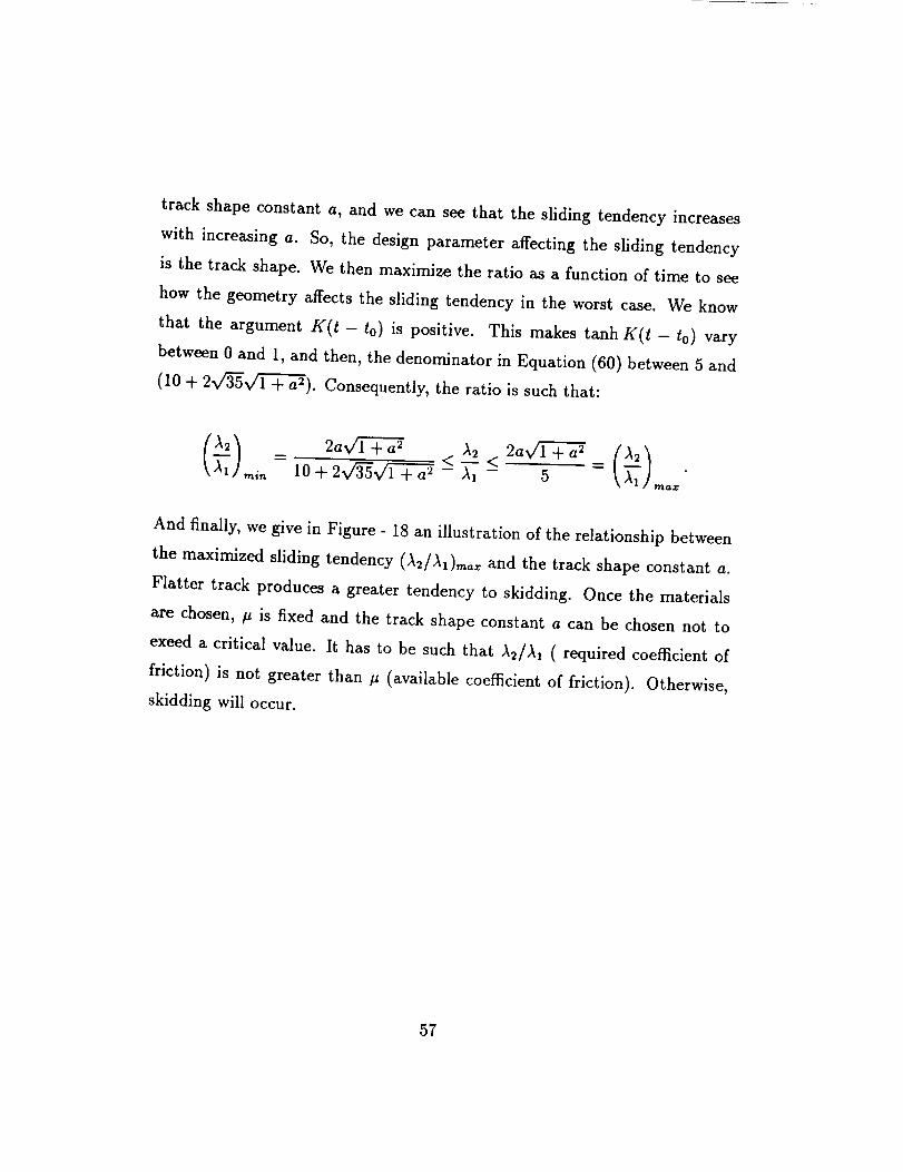
track shape constant a, and we can see that the sliding tendency increases

with increasing a. So, the design parameter affecting the sliding tendency

is the track shape. We then maximize the ratio as a function of time to see

how the geometry affects the sliding tendency in the worst case. We know

that the argument K(t - to) is positive. This makes tanh K(t - to) vary

between 0 and 1, and then, the denominator in Equation (60) between 5 and

(10 + 2v/_v_ + a2). Consequently, the ratio is such that:

Z = 10+ lvT--- < - < ++ - A1 - 5 = _ ,,,_="

And finally, we give in Figure - 18 an illustration of the relationship between

the maximized sliding tendency (X2/X1)m_ and the track shape constant a.

Flatter track produces a greater tendency to skidding. Once the materials

axe chosen, # is fixed and the track shape constant a can be chosen not to

exeed a critical value. It has to be such that $2/$i ( required coefficient of

friction) is not greater than tt (available coefficient of friction). Otherwise,

skidding will occur.

57

45 _''" ' , i , , , i ' , , i " ' ' i ' , , I , , ,

/35

25

( Z1 / Z2 ) max

_'_ , , , I , , , I , , , I , , , I" 5 I I I

4

0 /'2 4 6 8 10 2/

a acritical

Figure - 18. Required coefficient of friction versus

the track shape constant.

58

Chapter 4

ANALYSIS OF THE CATCI-]:ING

PROCESS

The ball, launched from the primary centrifuge according to the process

described in detail in the previous chapter, is then caught on the second

centrifuge. The resulting momentum transfer is used to propel this centrifuge.

4.1 CATCHING CONDITION

For a maximum momentum exchange, the velocity vectors of the points of

impact on the ball and the rotating blade must be equal to insure no bounc-

ing, nor sliding of the ball on the track. The normal components of the

two velocity vectors have to match so that the ball does not bounce off the

track, and the tangential components have to be equal to insure no sliding

of the ball on the track. This catching condition can be summarized by the

following equation:

v] - v_ - 0, (61)

59

where, vl is the velocity of the tip of the ball, and v: the velocity of the

impact point on the track where the ball is to land. Solving Equation (61)

will allow us to determine the exact position and timing for catching.

4.2 DETERMINATION OF CATCHING P OSITION

AND TIME

At the exit of the primary launcher, the center of mass of the ball has a linear

velocity v,_it, as mentioned in the previous chapter. The ball is also rotating

at a rate & as explained before.

have a velocity v_ such that:

This makes the impact point on the ball

v_:_it_usin- (u cos _ ) , (62 )

where the angle ( is defined in Figure - 18 and u is the rotating speed,

from Equation (24) in the previous chapter, differentiated once with respect

to time. This can be, equivalently written as:

(/;u = + ÷1. (63)

Substituting for ÷l from Equation (47), also in the previous chapter, taken

at the exit of the track, we can write:

u= (64)

6O

The velocity of the point of impact on the rotating track is:

_ = ( v_la_ - r°we_<sin(wt + () ) (65)rowe _ cos(wt + _)

where v,,t_v is the linear velocity at which the relay is moving. This velocity

vector is obtained by differentiating with respect to time the position vector

of the impact point on the blade,

F=(v_*i_vt+r°e_¢c°s(wt+_))roe*¢ sin(wt + _) " (66)

We have to keep in mind while differentiating that we are only interested in

one point, the impact point. This means that ( is not a variable here. It has

a specific value that we have to solve for ¢_.

From Equations (61, 62, 64) we get:

v_._.ti_. - u cos ( = -_r0e _¢' sin(wti + (1), (67)

and

- usin_ = ovroe _¢' cos(tvt_ + ¢i), (68)

where 73relative is the relative speed of the two moving bodies (ball and relay),

tJrelative -- ,3exit -- Urelalt _ (69)

and ti is the time at which the ball impacts the track.

When we solve Equations (67, 68) the catching parameters, position on

the blade, _i and time at which catching occurs, ti will be determined.

61

From Figure - 19,wecanseethat:

dz dz/d('

where

and

Then,

x = roe a_ cos(¢ + tot),

y = roe a¢ sin(C" + wt).

tan _1 + a tan(_ + cat)

a - tan(_ + cat) "(70)

Let us now consider the following identities:

and

1cos_ = 4-

V/1 + tan 2

1sin _ = +

_/1 + cot 2 _"

Usingthe relationship between (tan_) and (tan(¢ + cat))expressed in Equa-

tion (7O),(cos_) and (sin_) can be rewritten as:

(a - tan(¢ + cat))cos_ = +

V/(1 + a2)(1 + tanZ(C + cat))

and

62

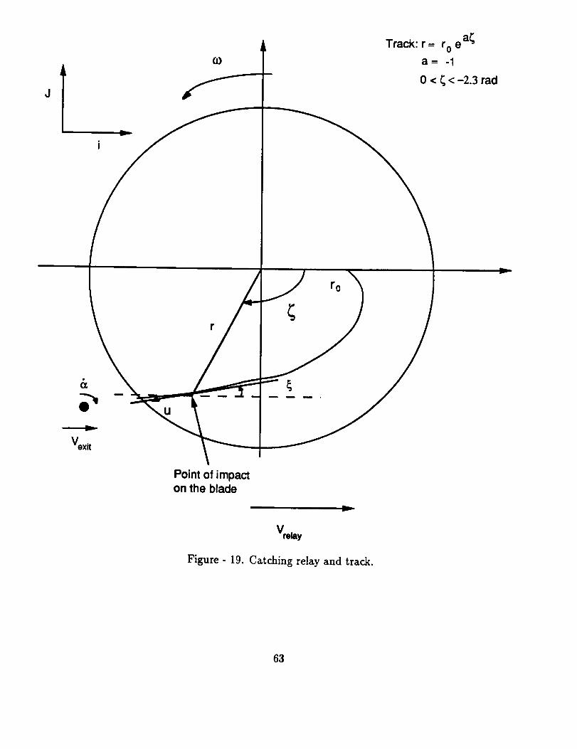
J

CO

Track: r = r o e a'=_"

a= -1

0 < _ < -2.3 rad

ro

v

&

Point of impacton the blade

ii,...--

Figure - 19. Catching relay and track.

63

sin _ = -4-(1 + a tan(( + _,t))

V/(1-4- a2)(1 + tan2(_ -t- wt))

Now, substituting for (cos_) and (sin_) as above in Equations (67, 68), we

get:

u(a - tan(Ci + wti)) = -rowe a_' sin(w(i + (i),

v,e,ati,_e _ V/(1 + a2)( 1 + tan2(( i + wti))

(71)

and

=(1+ atan((, + _t,)) = ro,_<' ¢os(_t,+ _,).=F _/(1 + aU)(1 + tan2(_i + wti))

Dividing Equation (71) by Equation (72) we get:

(72)

v,_t_t,,_<(1 + a2)(l + tanS((/+ wti))

:F u(l + a tan((i + wti))

a - tan((/+ wti)+

1 + a tan((_ + wt_)

= - tan((_ + _tO. (73)

This can also be written as:

q:-U 1 + a tan(_i +¢oti)

a(1 + tan2((i + wti))

1 + a tan(_ + wt_)

or simply,

T--l_relative

tL a- _ + tan2((i + wt,). (74)

64

If we square this equation, we can solve for tan(Ci + wti) as:

tan2((i +wti)= (v'e_ti_'e) z (1 + aJ-_) - 1. (75)

Now, we can go back to Equation (72) and rewrite it using the identity:

cos(¢_+ _t_) = +V/1 + tan2(_i + wti)

The equation then becomes:

.(i + a tan(¢_ +_t,))= rowe °c", (76)

or, if we want to solve for _i,

(i = al_ln [ u(l+atan(_+wti))](77)

where, tan(_'_ + wt_) is given by Equation (75). The solution, ¢'i, gives the

position of the ball on the track at catching. We can also solve for the

argument (wt_ + (i) of the tangent from Equation (75), and finally deduce t_,

the time at which catching must occur. This time can be written as:

ti=- arctan 1+_-_ -1 -(i+kTr , (78)od

where, k is chosen so that the catching time is greater that the time the ball

exits the launcher.

65

4.3 NUMERICAL APPLICATION

Let us now consider again the practical system proposed in the previous

chapter and determine the position and time of catching. Let us assume at

this point that the second centrifuge is not moving yet. It is just rotating at

the same angular rate w as the primary launcher. Consequently,

v,._t,,ti,_, = v,=it = 1.7 km/s.

We can also have from the previous chapter (Equation (47)) the value of ÷

at the exit, which is, ÷1 = 595 m/s for the particular example analyzed in

the previous chapter. Substituting for ÷1 in Equation (63), we can determine

the value of u as:

u = 841 m/s.

We also have:

• r0=0.01 m,

• and w = 10000 rad/s, as before.

• The track shape is the same as for the launcher case but its orientation

is different, and so the constant has a different value. For the catcher,

the track shape constant is a = -1.

After substituting for u, Vrel,,ti,_,, to, w, and a in Equation (75) we get:

tan2((_ + wt_) = 7.17,

or,

tan(_'i + wti) = +2.68.

66

Now,substituting this result in Equation (77), wering the catchingposition:

_i = -2.3 rad,

which representsthe edgeof the track. This result confirms our intuitive

feeling that the ball had to be caught on the edgeof the track to satisfy

the velocitiesmatching asexplainedbefore. Finally, wecansolvefor ti from

Equation (78):

ti = 1.3 ms,

where k was taken equal to 3.

Knowing the total time of the launch sequence tl = 0.9 ms from the

previous chapter, we can deduce the time of flight of the ball between the

two centrifuges. This time is:

t flight = ti -- tl = 0.4 ms.

And knowing the velocity at which the ball is travelling, we can deter-

mine what distance, d, initially we should place the relay from the primary

launcher:

d = Yezit tltigat = 0.68 m.

It is better to start with an initial separation of about 500 m to insure that

the time the ball spends on the relay is very small compared to the total time

of flight of the ball for kinematics studies purposes as we shall see later. The

ball will then be caught several revolution later than the time ti calculated

above. We have to choose k such that the time of flight will correspond to the

desired distance. This fact will not be taken into account in this chapter. We

will consider the minimal separation between the launcher and the relay of

0.68 m, but we will make the necessary changes in the generalization chapter

for multiple balls launching.

67

To conclude this section on the catching conditions, we illustrate the

orientation of the track both at t = 0 and at t = ti in Figure - 20 and

Figure- 21.

4.4 BEHAVIOR OF THE BALL ON THE CATCI-_R

Now that the first ball is caught smoothly at the edge of the blade without

any bouncing or sliding, we have to determine its trajectory on the track.

As for the launch process, Lagrange equations with multipliers are used to

analyze the behavior of the ball on the centrifuge. The same constraints as

before are on the system. The first specifies the track shape and the second

insures that the system is conservative by constraining the ball to roll on the

track. Equations (10) through (21) from Chapter 3 still apply, although the

orientation of the angle ( and the track shape constant a are different in this

case. The reader should refer to Figure - 19 where an illustration of the track

on the catching rotor was given.

Equation (21) from the previous chapter gives in this case:

This equation can be integrated and, along with the initial condition, s = 0

when r = ra, it gives a relationship between the track length and the radial

position of the ball:

s(t)= (_ (rx--r). (80)

Then, the second constraint equation becomes:

f_=ga(t)+(_(r(t)-rl)=O. (81)

68

Figure - 20. Orientation of the track on the relay at the

instant t = 0.

69

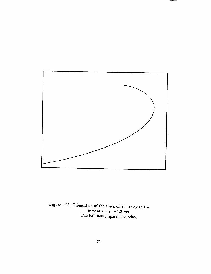
Figure - 21. Orientation of the track on the relay at the

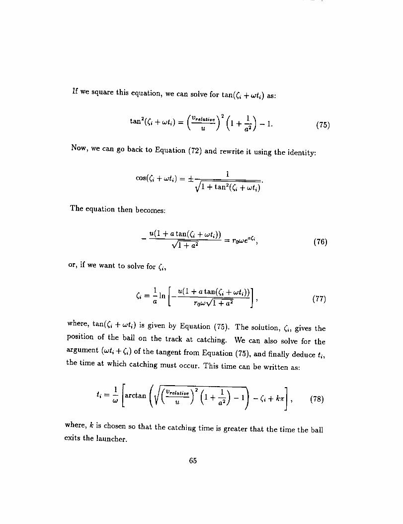
instaat t -- ti = 1.3 ms.

The ball now impacts the relay.

7O

The equationsof motion turned out to be exactly the sameasfor the launch

process,and the governingequation is:

r(t) = A cosh K(t - ti) + B sinh K(t - ti). (82)

The initial conditions at catching are known in terms of position and velocity:

r(ti) = r,,

and

v(t_) = v...,

for the center of mass.

Now, from v(ti) we can get ÷(t;). We have:

v2 =÷2+r2@+_)2,

from Equations (10, 11) of the previous chapter. We can also use the rela-

tionship between _ and ÷ as expressed in Equation (33) in Chapter 3 and

the previous equation becomes:

v 2=÷2 1+_-_ +r2w 2+-r÷w,a (83)

or_

2r÷w + r2w 2 - v 2 = O.a

The solution to this equation is:

--2r_ + ,/-5÷= o , (84)

where D is defined as:

D=4[v2( 1 +a _) -r2w2] • (85)

71

Equation (84) can be expressed as:

-arw 4- a_/v_(1 + a s) - a_r_w _÷= (86)

1 +a 2

At t = ti we get:

-ar, w + a_/v_'xi,(1 + a 2) - a2r_w _÷(ti) (87)

1 +a 2

where the "+" sign was chosen over the "-" sign because ÷(ti) has to be

negative since r(t) is decreasing from rl, radius of the rotor, to r0 near the

center. We also know that the track shape constant a is, in the case of the

catcher, negative. It turns out that:

= -÷,,

where ÷1 is the value of ÷ at the end of the launch sequence (at time tl).

Now, from Equation (82) we can write:

r(ti) = A.

Differentiating Equation (82) with respect to time and setting t = ti we can

also write:

÷(t,) = BK.

Identifying these two equations with the initial conditions at catching as

expressed before we get:

A= FI,

72

and

K

The trajectory of the ball on the catcher blade is given at all times by:

r(t) = r, cosh K(t - t,) - -_ sinh K(t -ti). (88)

Let us denote the time it takes for the ball to reach the center of the rotor

by t2. Solving Equation (88) at the center (r(t) = r0) gives the value of the

interval of time (t2 - ti). This interval of time is the time actually spent by

the ball on the track of the catching rotor while t2 is the total time from the

very beginning of the launching process (t = 0).

The ball is now going to be transferred to another track on the catcher

and then be propelled forward or backward. For the purpose of this partial

study, we will only consider throwing it back to the primary launcher.

4.5 RETURN OF THE BALL TO THE PRIMARY

LAUNCHER

The ball is now on the second track of the catcher to be propelled backward.

The track shape is always the same and the orientation is opposite to the

track where the ball is caught making it similar to the track where the ball

is accelerated on the primary launcher. The trajectory of the ball is then

known. We just need to replace to in Equation (41) (Chapter 3) by t3 and

we can write:

r(t) = ro cosh K(t - t3), (89)

73

where t3 is the time at which the ball leaves the center of the catcher and

starts rolling back off toward the edge.

The position and the velocity of the ball as functions of time are described

in Equations (42, 43) in the previous chapter. We also need to satisfy Equa-

tion (50) from that chapter to insure that the ball leaves exactly backward

(horizontally).

Let t4 denote the time at which the ball leaves the edge of the catcher. We

can find the value of this time by solving the condition expressed in Equa-

tion (50) mentioned before. This condition has been developed in Chapter 3,

we will then just use the result in Equation (57) (previous chapter), where we

replace tl by t4. The value of k is adjusted so that the results are physically

acceptable. The value of t4 has to be greater than (t2 + (t4 - t3) ). The value

of (t4 - t3) can be determined by solving Equation (89) at the edge where

t = t4 and r(t) = rl.

Finally, (t 3 - ti), the transfer time between the two tracks and possibly

some extra delay time where the ball is maintained near the rotor axis to

insure proper orientation of the centrifuge, can now be deduced knowing

(t4 - t3), t4, and ti.

4.6 PRACTICAL CAS_

This is a continuation of the practical case considered previously. Let us use

the same specifications as before for the centrifuge:

• rl = 0.1 m,

• ÷I = 595 m/s,

• K = 5976.

74

The trajectory of the ball on the track is described by:

r(t) = 0.1 cosh K(t - ti) - 0.099 sinh g(t - t,).

Figure - 22 shows the position of the ball as a function of time. r(t) decreases

from rl to r0 in an interval of time (t2 - ti) = 0.5 ms.

Knowing ti from the previous section, ti = 1.3 ms, we can now deduce

t2. So, the total time for the ball to reach the center of the catcher from the

time we start spinning the centrifuges is t2 = 1.8 ms. The position of both

tracks is represented at this time in Figure - 23 and Figure - 24.

We also illustrate ÷(t) versus t in Figure - 25. The mathematical expres-

sion for ÷(t) as a function of time is:

÷(Q = 597.6 sinh K(t - t,) - 595 cosh K(t - t,).

It starts at -÷1 = -595 m/s and reaches the value -4.25 m/s after 0.5 ms

which gives a velocity value of the center of mass, according to Equation (83),

of 104.33 m/s at ro near the center of the rotor ( about 6% of its initial value).

This should help the transfer to the second track.

Now, before we can determine how long the ball is going to be kept near

the center, we can calculate the interval of time (t4 - ta) as explained before.

We find:

t4 -- t3 = 0.5 ms,

still the same time as before since the ball is rolling from r0 at rest, to the

edge, rl.

The next step is to calculate t4 knowing that it has to be greater than

2.3 ms. The result is:

t4 = 2.48 ms,

with a value of k equal to 9.

75

0.1

r(t)

0.08

0.06

0.04

m

0.02

0

0

, I I I , I

1 2 3

!

!

m

u

4

K(t-t i)

Figure - 22. Radial position of the ball on the relay.

76

J

Figure - 23. Orientation of the track on the relay at the

instant t = t2 = 1.8 ms.

The ball is now at the center of the relay.

77

Figure - 24. Orientation of the 2"d track on the relay(accelerationpart) at the instant t = t2 = 1.8 ms.

The ball is now being transferred to this track.

78

r(t)

100

-40

-180

-320

-460

-600

0 2

K(t-t i)

3 4

Figure - 25. Variations of ÷(t) from the catching

point to the center of the relay.

79

And finally, wecan deducet3:

t3 = 1.98 ms.

From the instant t_ to the instant t3, for 0.18 ms, the ball will be trans-

ferred to the second track and will be kept there until the end of this time

interval, when a new acceleration sequence begins. An illustration of the

position of the track at this particular moment is given in Figure - 26. The

ball is now released from the center.

The total time for the ball to be accelerated, launched, caught, and for it

to roll back off the catcher to its edge is 2.48 ms. It leaves with a velocity of

1.7 km/s backward. An illustration of the rotor blade from where the ball is

going to be launched backward at that particular time is given in Figure - 27.

Assuming that the catcher is still at the same distance from the primary

launcher after this first ball catching, the time of flight between the two

centrifuges is still 0.4 ms as before. This means that the total time it takes

for the first ball to be launched and collected back by the primary launcher

after it accomplishes its mission is 2.88 ms.

At this point, we can determine the momentum transferred by this first

ball to the relay it impacted. We found here that gout = -_i,,, which means

that the decrease in the ball velocity as defined in Chapter _2, becomes:

and the momentum gained by the relay is:

M(P'o_, - _,,) = 2rag,,,.

(90)

(91)

In the particular case considered, the numerical value of this momentum

gain is 14 kg m/s, if the ball weighs 4 grams (0.5 cm radius steel ball).

Furthermore, if the relay is 10 kg, then the velocity increment is 1.4 m/s.

8O

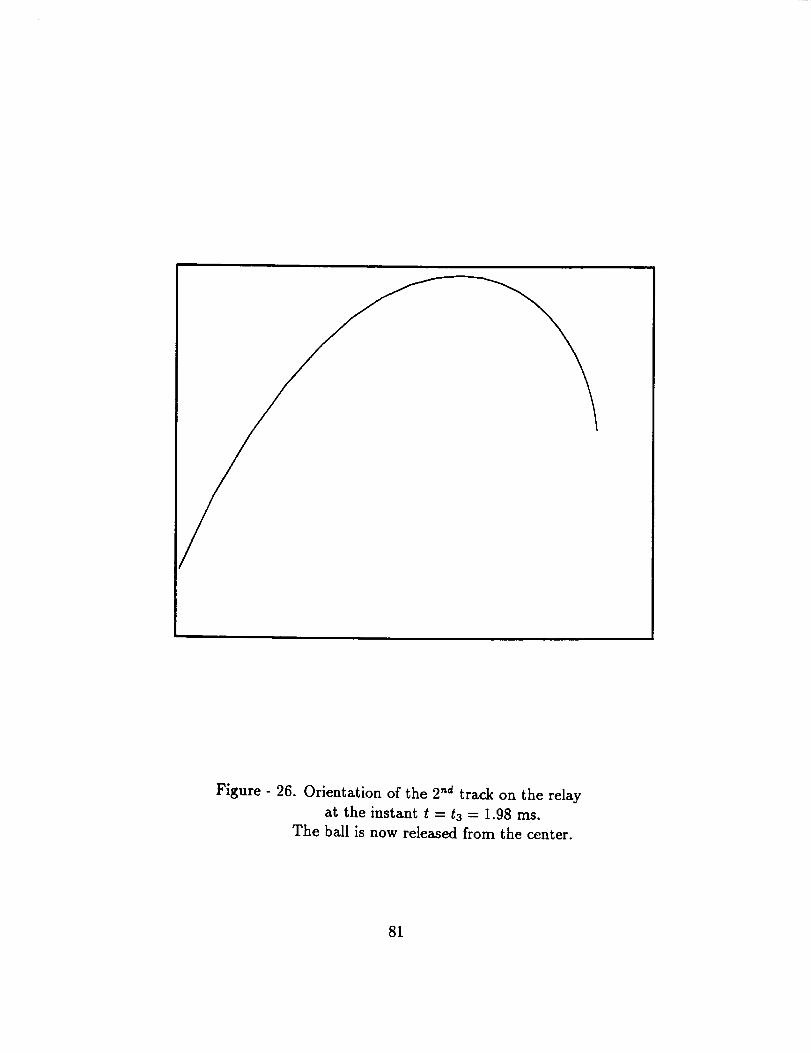
Figure - 26. Orientation of the 2"d track on the relayat the instant t = t3 = 1.98 ms.

The ball is now released from the center.

81

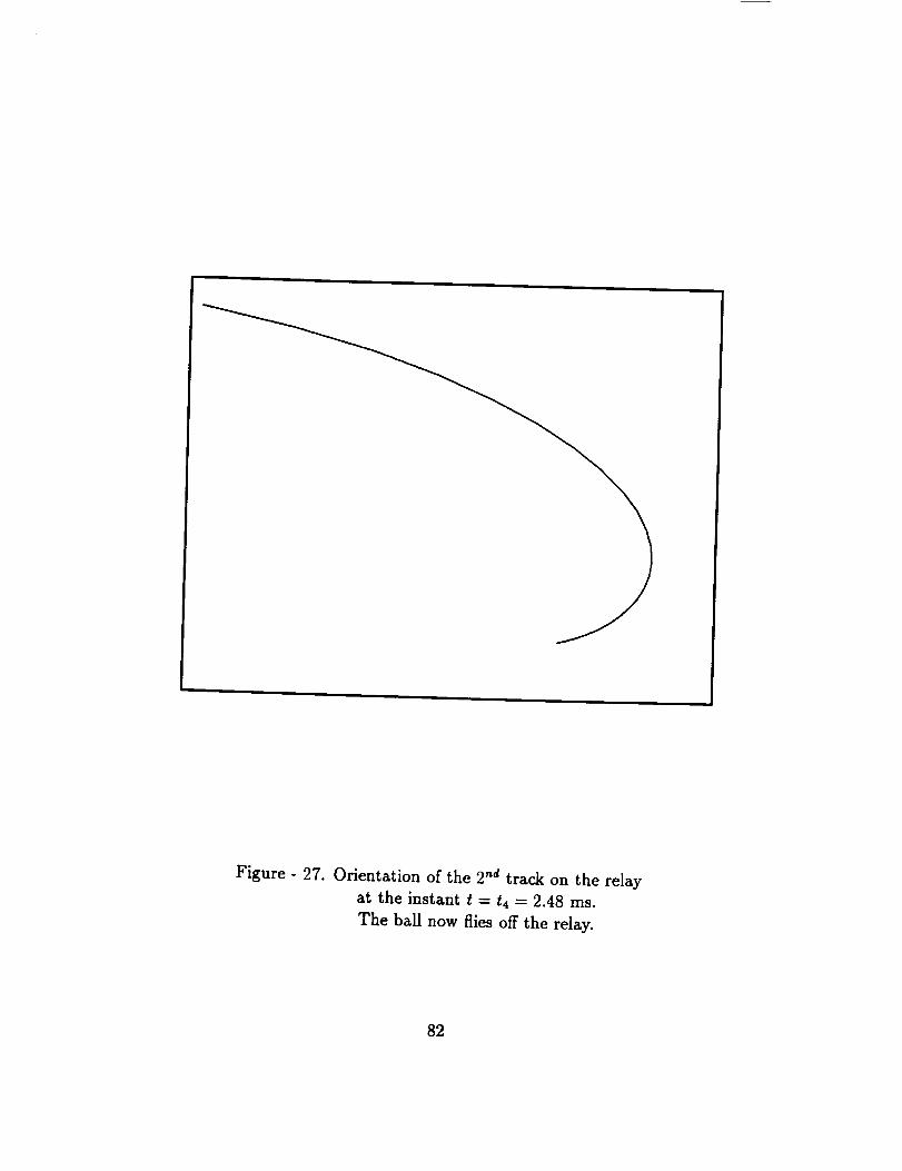
Figure - 27. Orientation of the 2"d track on the relayat the instant t = t4 = 2.48 ms.

The ball now flies off the relay.

82

Now, in terms of angular momentum,we have:

L. = x

and

= x m(-,,..).

(92)

(93)

This means that the angular momentum of the ball before and after the

interaction with the relay is exactly the same and Af_,roto,. = O. There is no

angular momentum gained by the rotor after the launch of this first ball. This

can be explained by the fact that the ball transfers all its angular momentum

to the relay when it lands on the track and rolls up to the center of the rotor

where it stops. So, in order for the ball to be accelerated on the second

track and leave with the same velocity it impacted the relay the first time,

the ball gets back the angular momentum it previously transferred to the

relay. Therefore, the relay gains /,in in a first step, and then loses f-,out in

a second step, which is exactly the same quantity, leaving it with zero net

angular momentum gain. This is not necessarily the case for the next bails

launched. It depends on whether or not the ball is leaving with exactly the

same angular momentum it had when it impacted the relay. This in turn,

depends mainly on the position where the ball is caught on the track of the

relay and where it exits this relay.

83

Chapter 5

GENERALIZATION: 1VIULTIP LF,

LAUNCH ANALYSIS

After the detailed analysis of the launching and the catching of the first

ball, as described in Chapter 3 and Chapter _ respectively, we are now to

consider multiple balls launching and catching, until our objective of acceler-

ating the relay to the desired speed is achieved. We will start by generalizing

the results obtained in Chapter 3 to describe the acceleration of the nth ball

on the primary launcher. We will then describe the catching position and

time, and the behavior of the nth ball on the relay, based on our analysis

in Chapter _. We will also give the velocity increments the relay is getting

from its impact with the nth ball. All these results are to be coded in a

computer program that would keep track of all the information conserning

the acceleration of the spaceborne relay.

5.1 LAUNCH OF. BALLS

We can determine at this point the frequency of launch of the projectiles.

The maximum frequency would be just the same as the frequency of the

rotational movement of the centrifuge, which is in the case of the application,

84

1.59kHz. This meansthat we launch one ball per revolution. However,we

will consider launchingoneball every two revolutions instead, to makesure

that the previous ball had enoughtime to leavethe relay, when the newly

launchedball impacts it. When the track is in the right position to launch

the first ball, which is t = 0.4 ms in the particular case considered before, we

wait for exactly two revolutions (1.26 ms) and release the second ball. The

time would then be t = 1.66 ms. The first ball would have already left the

launcher. It will also take this second ball 0.5 ms to get to the tip of the rotor

and it will leave at t = 2.16 ms. We can generalize this result and state that

soon after one ball leaves the launcher, another one is released near the center

of that launcher. The exact value of this time delay between the exit at the

tip of the rotor of one ball and the release of the next one, is determined by

the difference between two periods of rotation of the centrifuge and the time

it takes the ball to reach the tip of the rotor when it is accelerated from the

center. The n th ball will be released near the center at a time treuo_e:

t..,eo..= (0.4+ x.26(. - 1))ms,

in the case of this application, or in general:

t,_le.oe= to+ 2 (n - 1) T, (94)

and it will leave the track at

te_t = (0.9 + 1.26 (n -- 1)) ms,

in this particular case, which can also be generalized as:

t.xit = q + 2 (n- 1) T (95)

85

5.2 VELO CITY OF THE RELAY AFTER THE LAUNCH

OF THE nTH BALL

Based on our kinematics calculations in Chapter ,_, the velocity of the relay

after the launch of the nth ball would be given by Equation (8) in that

chapter, where Vi_ would be the relay velocity after the (n - 1)th ball leaves

heading back to the primary launcher. We can just put that equation in a

loop specifying the initial velocity of the relay, which is zero (starting from

rest), and the program will give us the velocity of the relay after each ball

leaves it.

5.3 DETERMINATION OF THE CATCHING PO-

SITION AND TIME FOR THE nTH BALL

As we mentioned previously, we want an initial separation of about 500 m

between the primary launcher and the relay. Therefore, when we code Equa-

tion (78) (Chapter _) in the program, we keep on increasing the value of the

integer k until the corresponding catching time, ti, is such that the time of

flight of the ball, t11i_ht , corresponds to a distance of at least 500 m. This

will set the initial distance. Then we will solve Equation (78) mentioned

above, to get the time at which the nth ball must be caught, and k would

be chosen so that the result is physically acceptable. This means that the

time of catching needs to be at least equal to the time the nth ball exits the

launcher, plus the time of flight, which can be formulated mathematically as:

ti :> $ezlt + t fllght

For the determination of the catching position, we just solve Equation (77)

as explained before in Chapter 4, and we will find the angular position, _i, of

the ball on the track at the impact point. It is important to note here that

86

one condition has to be met when solving Equation (77). This condition is:

1 + a tan(_'i + wti) < O. (96)

This condition was not mentioned before in Chapter _t because it was satisfied

in the case of the first ball, in the particular example considered. However,

since we are generalizing the results in this chapter, we will have to check

this condition and make sure it is satisfied. The first ball is caught at the

edge of the track, but, as we will see later from the results of the computer

program, the second ball will be caught slightly away from the edge, toward

the center. Actually, the difference in angular position, ¢i, of the second ball

catching point and the first ball is very small (one thousandth of a radian).

This difference between two successive bails is very small, but between the

1st and the nth, it will be quite large. The catching point will move farther

and farther from the edge, until it becomes, eventually, near the center of

the relay, when this one is moving at a speed comparable to the speed of

the incoming balls. Therefore, tan(C; + wti) will change a great deal from

the value calculated for the first ball, and we want to make sure that it

always satisfies the condition expressed in Equation (96) above. Otherwise,

catching cannot be achieved. The system of Equations (71,72) from the

previous chapter, will not have a solution, and the catching condition of

matching velocity vectors at the impact point would be impossible. It turns

out, after we run our program, that this condition (Equation (96)), limits the

number of balls launched to 882 in the case of the specific example treated.

This represents actually a little more than 1/10th of the total number of bails

needed to get the relay going at a velocity almost equal to the velocity of

the incoming balls ( v_,t_ = 1.698 km/s for n = 8000, and vb_u = 1.7 km/s).

This number of balls will indeed be sufficient the accelerate the relay to more

87

than half the velocity of the balls. The relay velocity obtained with n = 882

is vr, l_v = 861 m/s. This is the limit of what we can achieve. A display of the

catching position of the last ball is given in Figure - 28. We cannot possibly

launch and catch more balls unless we change the parameters of the system,

namely, the track shape. We tried a more circular track, with a constant

a = 0.5, to improve the velocity of the relay, but the change would not be

dramatic. The exit velocity of the balls would be in this case v,_t - 1792

m/s, and the maximum number of balls we can catch smoothly would be

n = 946. The resulting relay velocity would then be v_,l_y = 951 m/s. A

display of this track is given in Figure - 29. We chose to keep the previous

case, a - 1, since the improvement is not very important compared to the

trouble that we may have for mechanical design: machining a multiple tracks

rotor as shown on Figure - 30.

5.4 BEHAVIOR OF THE .TH BALL ON THE RE-

LAY

The nth ball will go through two different stages depending on which track

it is on. At first, it will roll up the track from the catching position and stop

at the center of the relay. Then, it will be transferred to the second track,

where it will be accelerated and roll back toward the edge of the relay. It will

fly off the track and go back to the primary launcher. We will now consider

these two cases separately.

5.4.1 From Catching Position to Center of Relay

The first ball being caught at the edge of the relay, will roll for 0.5 ms to

reach the center, which is the same as the time it takes the ball to reach the

edge when accelerated from the center on the primary launcher. However,

88

First ball

Last ball

v

Figure - 28. Catching position of the first and the last ball launched.

89

Figure - 29. Logarithmic spiral track with a track shape constant a = 0.5.

90

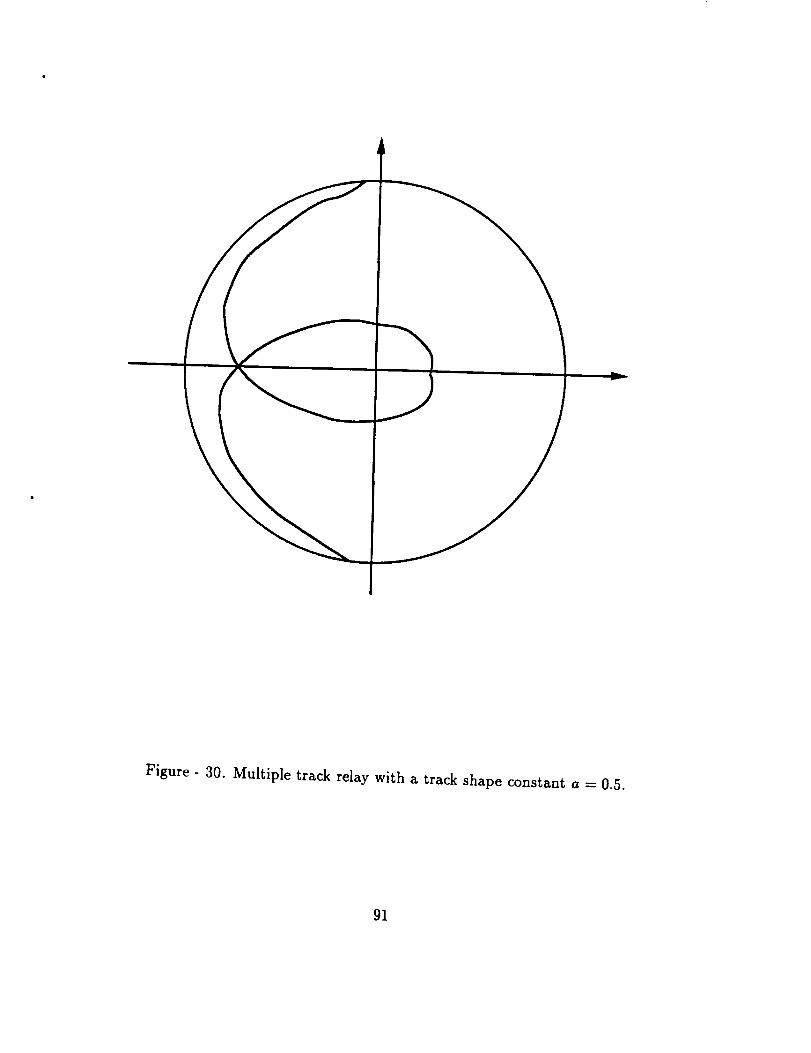
Figure - 30. Multiple track relay with a track shapeconstant a = 0.5.

91

for the secondball, since it is caught a little farther from the edge, toward

the center, the time neededfor it to reachthe centerwill beslightly shorter,

and for the next ball, it will be even shorter, and so on, until the last ball

launched. To find the exactvalueof this time, weneedto solveEquation (88)

in Chapter 4, where we replace rl by r_, and -÷t by ÷_ for the general case

of the nth ball. The equation becomes:

r(t) = ri cosh g(t - ti) + -_ sinh g(t - ti). (97)

One way to solve this equation analytically would be to use the following

identity:

cosh 2 x - sinh 2 x = 1,

or,

sinh x - i y/cosh2 x - 1.

Now, since the argument of the hyperbolic sine in our case, K(t - ti), t being

the time we are solving for, is positive, sinh K(t - ti) is also positive. There-

fore, we will chose the "q-" sign over the %" sign in the expression above.

Now substituting for sinh K(t- ti) as explained above in Equation (88) men-

tioned earlier, we get:

r(t)=ricoshg(t-t,)+ r_/cosh_K(t-t,)-l. (98)K

Let us denote cosh K(t -t_) by X, for simplification purposes• Then, Equa-

tion (98) can be written as:

or,

r(t)=ro=riX+K.__ -1'

r0 - r_X = nvZX2 - 1.K'-

(99)

( oo)

92

We can square both sides of Equation (100) and rewrite it as:

\K s- \KS +r°_ =0.

The solution to this equation is:

(101)

where A is given by:

--ror_± V_x = _ , (102)

K 2 tK 2

We would note here that we have to chose the positive root only since X

represents the hyperbolic cosine, which is always positive.

The next step is to solve for the argument, K(t - ti), of the hyperbolic

cosine. Let us call this argument x. we can write:

e x + e -xX=

2

If we denote e_ by Y, we can write the equation above as:

or simply,

y2 _ 2XY + 1 - O.

The solutions to this equation can be written as:

(103)

y = x + _"i _ l.

We have to keep in mind that Y has to be positive, since Y = c_. We

will chose the "+" sign in the above. One could argue that the root with

the "-" sign is also positive. But, even when positive, it will be a relatively

93

small number, which in turns meansthat the argument of the exponential,

x = K(t - ti), would be negative. And this last statement is not physically

acceptable. Therefore, we will chose the larger solution of the two, which is

the one with the "+" sign.

We can finally write the time the needs the reach the center of the relay:

1 [X + _, (104)t - ti = _ In

where X is as defined in Equation (102) above.

5.4.2 Acceleration of the nth Ball from the Center to the Edge

Now, the ball is being accelerated from rest on the second track, where it will

fly off the edge and travel back to the primary launcher. The orientation of

this track is similar to the launching track on the primary launcher (a = 1).

However, that track should be oriented such that the ball is launched back-

ward and not forward. There is a difference of 7r in the angular position

of the ball at the exit with respect to its position on the primary launcher.

The time it takes the ball to reach the edge is, as determined before, 0.5 ms,

and it will be the same for all balls. The exit time can be calculated from

Equation (57) in Chapter 3. The value of k would be chosen so that the value

of the time obtained here is greater than the time it takes this nth ball to

reach the center, calculated in the previous section, plus the 0.5 ms needed

to reach the edge of the second track when accelerated from the center of the

relay, as explained in the beginning of this paragraph. We will also note that

we start here with a value of k = 1, instead of 0 as in the case of the primary

launcher, to take care of the orientation of the track that has to insure a

backward launch.

94

5.5 POSITION OF THE RELAY

We need to determine the exact position of the moving relay when the nth

ball is about to impact it. After the (n - 1)th ball leaves the relay, this latter

would be moving at a velocity already determined (second section of this

chapter). Therefore, the distance it travelled from the time the (n - 1)th ball

left it, until the nth ball arrives, can be easily determined. This relay position

should be compared to the distance that the nth ball travelled, from the time

it exit the primary launcher, to the catching time. If the distance travelled by

the ball is larger, as we will see from the results of the program, a mechanism

should be included to slow down the ball for exact timing. This is one of

the purposes of the guidance system. As we will describe it in details later,

all three directions of motion would be corrected by the aiming mechanism.

Vertical adjustment will insure the catching of the ball at the desired position,

¢i, and a longitudinal adjustment will insure a synchronization between the

incoming ball and the catching time on the relay.

5.6 ROTATIONAL ENERGY OF THE RELAY

The last part of this kinematics and dynamics study, would be to calculate the

change in rotational energy the relay experiences due to its impact with all

these little projectiles. For the first ball, caught and launched from the edge,

there is no change in rotation energy, as explained in Chapter _. However,

for the nth ball, caught at a position between the edge and the center of the

relay, and then accelerated all the way to the edge, the relay would lose some

rotational energy. Let us determine exactly how much energy it would lose.

95

We have:

and

We also have:

and,

_,_ = ( r;cos(wt; + ¢i) )ri sin(wti -t- _i) '

f'o_,= ( r' c°s(wt + (') )rl sin(wt + (_1) '

where t is the time the nth ball flies off the edge of the relay and all other

quantities are as defined previously.

Therefore, we can write the angular momentum as:

Lin "- -mriVin sin(wti + _i),

and,

Lo_, = rnrlvi, sin(wt + (1).

These two quantities can be easily calculated and the difference, Li,_ - Lo,,,

which is negative, represents the decrease in rotational energy after the nth

ball impacts and leaves the relay. We have to compile all the decreases of

energy, from the second to the last ball, to get the total lost of rotational

energy. We should then be able to deduce the change in angular speed of the

96

relay. We expect this change to be negligible, but we will calculate it in our

program.

We are now ready to write the general program that codes all the different

steps described in this chapter. We win mention though that we added one

more thing at the beginning of this program. It will check first the sliding

tendency based on the roll versus skid analysis in Chapter 3. If the ball

is expected to slide on the track, it will ask the user to change the system

parameters. Otherwise, it will inform him that the choice of parameters

is fine and that the ball will roll nicely on the track. It will then go on

calculating the data needed to summarize all the derivations and visualize

the propulsion of the spaceborne relay.

We will include in this section a summary of the results for the first 20

balls launched. Table - 4 will give the timing information, and Table - 5 the

positions information. The general code written is given in the appendix.

97

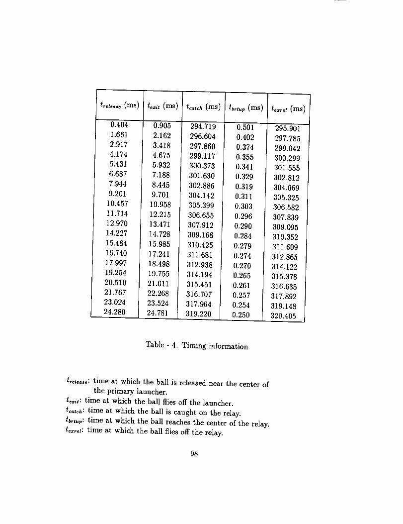
0.404

1.661

2.917

4.174

5.431

6.687

7.944

9.201

10.457

11.714

12.970

14.227

15.484

16.740

17.997

19.254

20.510

21.767

23.024

24.280

0.905

2.162

3.418

4.675

5.932

7.188

8.445

9.701

10.958

12.215

13.471

14.728

15.985

17.241

18.498

19.755

21.011

22.268

23.524

24.781

294.719

296.604

297.860

299.117

300.373

301.630

302.886

304.142

305.399

306.655

307.912

309,168

310.425

311.681

312.938

314,194

315.451

316.707

317.964

319.220

t .o, (ms)

0.501

0.402

0.374

0.355

0.341

0.329

0.319

0.311

0.303

0.296

0.290

0.284

0.279

0.274

0.270

0.265

0.261

0.257

0.254

0.250

te_e, (ms)

295.901

297.785

299.042

300.299

301.555

302.812

304.069

305.325

306.582

307.839

309.095

310.352

311.609

312.865

314.122

315.378

316.635

317.892

319.148

320.405

Table- 4. Timing information

t,¢_,_: time at which the ball is released near the center of

the primary launcher.

t_xi,: time at which the ball flies off the launcher.

tcatch: time at which the ball is caught on the relay.

tbrt,,p: time at which the ball reaches the center of the relay.

t_x_¢t: time at which the ball flies off the relay.

98

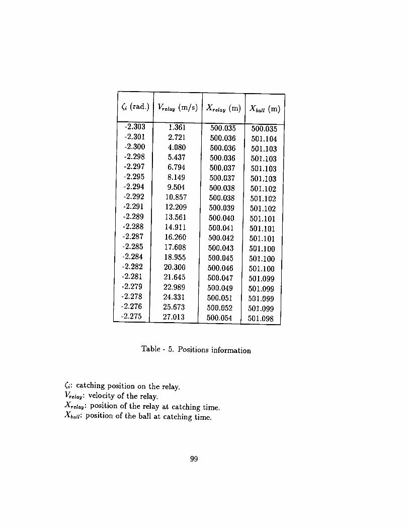
¢, (rad.)

-2.303

-2.301

-2.300

-2.298

-2.297

-2.295

-2.294

-2.292

-2.291

-2.289

-2.288

-2.287

-2.285

-2.284

-2.282

-2.281

-2.279

-2.278

-2.276

-2.275

(m/s)

1.361

2.721

4.080

5.437

6.794

8.149

9.504

10.857

12.209

13.561

14.911

16.260

17.608

18.955

20.300

21.645

22.989

24.331

25.673

27.013

500.035

500.036

500.036

500.036

500.037

500.037

500.038

500.038

500.039

5O0.040

500.041

50O.O42

500.043

500.045

500.046

500.047

500.049

500.051

500.052

5OO.O54

x o,,(m)

500.035

501.104

501.103

501.103

501.103

501.103

501.102

501.102

501.102

501.101

501.101

501.101

501.100

501.100

501.100

501.099

501.099

501.099

501.099

501.098

Table - 5. Positions information

(i: catching position on the relay.

V_elau: velocity of the relay.

X,_a_: position of the relay at catching time.

Xb_u: position of the ball at catching time.

99

APPENDIX

COMPUTERIZED COMMUNICATION AND

SYSTEM FOR SPACEBORNE CENTRIFUGAL

SPACECRAFT PROPULSION

CONTROL

RELAYS FOR

One of the most important engineering problems for this project consists

of accurately tracking the position of the projectiles and rotors and guiding each

projectile exactly onto the appropriate guide tracks on each rotor. We have to

control velocity vectors of the rapidly moving balls so that they encounter guide

tracks on the spinning rotors at just the right location and time. We need to

correct errors in lateral positions and make longitudinal adjustments to insure

that projectiles arrive at the next relay in proper synchrony with its rotation.

Guidance studies include the tracking mechanism (interrupt of optical

beam) and the aiming mechanism (electromagnetic focussing including the

electromagnetic deflection coils design and the switching circuitry). A

schematic of the system is given in figure 1.

@

i

.,, .,._

_,,_ 0

=,_

"_ "' II

[_, : ,

.'N-

Q

@

g

,]

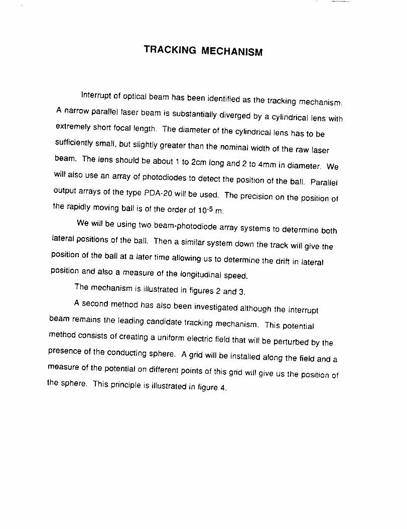
TRACKING MECHANISM

Interrupt of optical beam has been identified as the tracking mechanism,

A narrow parallel laser beam is substantially diverged by a cylindrical lens with

extremely short focal length. The diameter of the cylindrical lens has to be

sufficiently small, but slightly greater than the nominal width of the raw laser

beam. The lens should be about 1 to 2cm long and 2 to 4mm in diameter. We

will also use an array of photodiodes to detect the position of the ball. Parallel

output arrays of the type PDA-20 will be used. The precision on the position of

the rapidly moving ball is of the order of 10 -5 m.

We will be using two beam-photodiode array systems to determine both

lateral positions of the ball. Then a similar system down the track will give the

position of the ball at a later time allowing us to determine the drift in lateral

position and also a measure of the longitudinal speed.

The mechanism is illustrated in figures 2 and 3.

A second method has also been investigated although the interrupt

beam remains the leading candidate tracking mechanism. This potential

method consists of creating a uniform electric field that will be perturbed by the

presence of the conducting sphere. A grid will be installed along the field and a

measure of the potential on different points of this grid will give us the position of

the sphere, This principle is illustrated in figure 4,

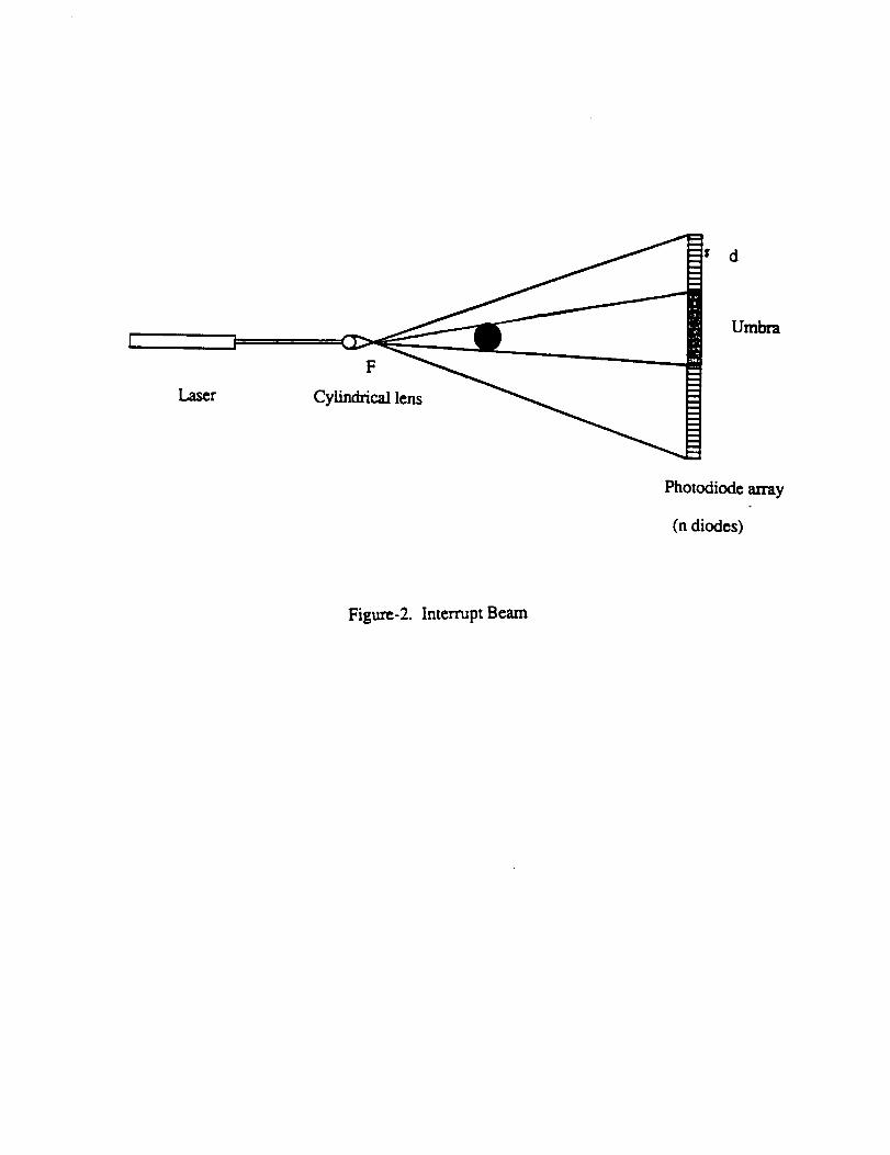
Lair

F

Cylindrical lens

d

Umbra

Photodiode array

(n diodes)

Figure-2. Interrupt Beam

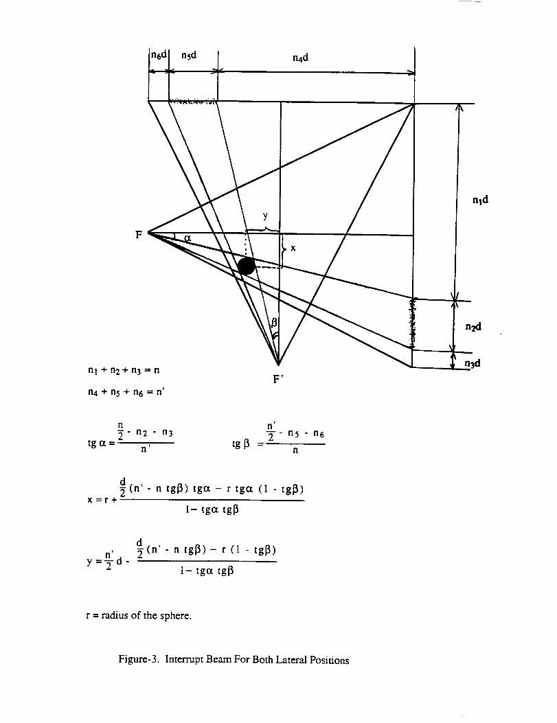
n4d

F

nl + n2+ n3 -- n

ml+n5+n6-n'

t

I'I rl'

_- n2 - n3 T" n5 - n6tg ot = n' tg 13 = n

d(n' - n tg13) tgct - r tgcx (1 - tg13)

x----r+I- tga tg13

n t

Y =Td -

d_(n'- n tg[3) - r (1 - tg13)

1- tgo_ tg13

r = radius of the sphere.

Figure-3. Interrupt Beam For Both Lateral Positions

+Vo

)):)

j_m

v

Eo

2L

-Vo

V(r,0) = -Eo (1 - (a/r)3) r cos0

Figure-4. Conducting Sphere in a Uniform Electric Field

AIMING MECHANISM

For the velocity trimming, we propose that the projectiles be directed

through a guide barrel after release from the centrifugal accelerators to limit the

dispersion of lateral velocities. We identified the concept of electromagnetic

focussing as the final aiming mechanism. When the ball arrives to the

correction circuit it will be magnetized. Its magnetic moment and the external

magnetic field that we create will produce a potential energy. A force will then

be acting on the sphere modifying its position. The velocity errors are expected

to vary randomly in magnitude and in direction from one projectile to the next

one launched. We need the switching time of the electromagnetic circuit to be

very small in order for us to set the necessary amount of magnetic induction in

the circuit to make the appropriate correction for each projectile. The first thing

we need to determine is the diffusion time of the magnetic field inside the

sphere to make sure that it will have enough time to get magnetized while

passing through the electromagnetic deflection coil at a high velocity. For this,

we solved Maxwell equations,

4_ 1 c3DVxH = -_ J + _- o_--t-

1 _B_TxE+ 0

c o_t-

V.D = 4/qo_7.B= 0

and got the diffusion equation,

oqB Vx(vxB) + _c2 V2B8t - 4_¢_

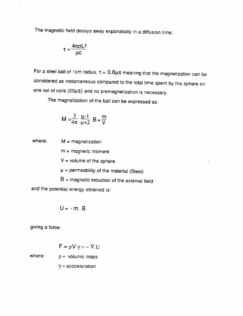
The magnetic field decays away exponatially in a diffusion time:

4_:cL 2

pc

For a steel ball of lcm radius, '_ = O.6#s meaning that the magnetization can be

considered as instantaneous compared to the total time spent by the sphere on

one set of coils (20#S) and no premagnetization is necessary.

The magnetization of the ball can be expressed as:

M=4__ I.t-1 B m#+2 = V-

where: M = magnetization

m = magnetic moment

V = volume of the sphere

p = permeability of the material (Steel)

B = magnetic induction of the external field

and the potential energy obtained is:

U= -m.B

giving a force:

where:

F = pV T = - V.U

p = volumic mass

"y = accceleration

3 _ V.B27 =_-_ _+2

This acceleration will compensate the error on the velocity"

v =vo-n_=O

Vo = initial error (about 0.1 m/s)

n = number of loops

The magnetic induction producing this acceleration is obtained when a

current l is circulating in a loop of radius a:

la 2

B=p.o 2(a2 + z2)3/2 (along the z-axis)

3 z

V.B 2 =- _ _ 02 I2a 4 (a 2 + z2) 4

Using N turns instead of one in every loop will make the current needed to

produce the same magnetic induction N times smaller. The total resistance R of

the coils (for one loop) is given by:

1R=Ro-

S

where: Ro = resistivity of the wire (copper)

I = total length of the wire

s = cross-section of the wire

The voltage necessary to produce the required current is:

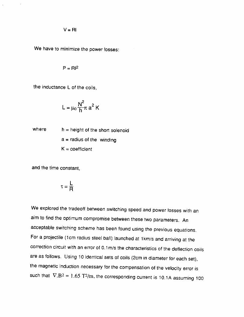
V=RI

We have to minimize the power losses:

P = RI2

the inductance L of the coils,

N2 2 KL = a

where h = height of the short solenoid

a = radius of the winding

K = coefficient

and the time constant,

We explored the tradeoff between switching speed and power losses with an

aim to find the optimum compromise between these two parameters. An

acceptable switching scheme has been found using the previous equations.

For a projectile (lcm radius steel ball) launched at lkm/s and arriving at the

correction circuit with an error of 0.1 m/s the characteristics of the deflection coils

are as follows. Using 10 identical sets of coils (2cm in diameter for each set),

the magnetic induction necessary for the compensation of the velocity error is

such that V.B 2 = 1.65 T2/m, the corresponding current is 10.1A assuming 100

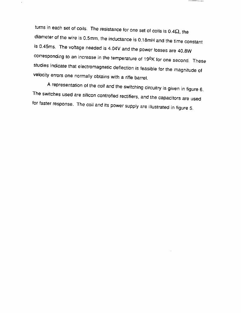
turns in each set of coils. The resistance for one set of coils is 0.4_, the

diameter of the wire is 0.5mm, the inductance is 0.18mH and the time constant

is 0.45ms. The voltage needed is 4.04V and the power losses are 40.8W

corresponding to an increase in the temperature of 19OKfor one second. These

studies indicate that electromagnetic deflection is feasible for the magnitude of

velocity errors one normally obtains with a rifle barrel.

A representation of the coil and the switching circuitry is given in figure 6.

The switches used are silicon controlled rectifiers, and the capacitors are used

for faster response. The coil and its power supply are illustrated in figure 5.

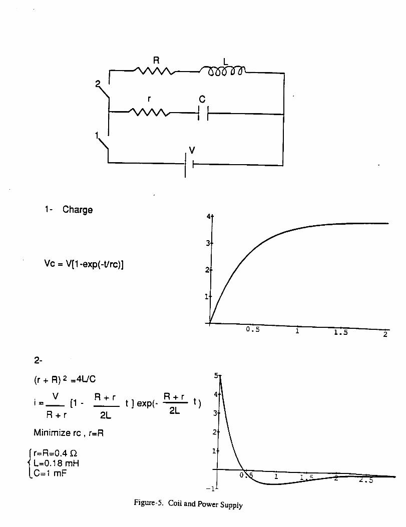
L

C

It

V

1- Charge

Vc = V[1-exp(-t/rc)]

4 _

,

2,

1

'5O. i!

1.5

m

(r + R)z =4L/C

V R+ri=___ [1 -

R+r 2L

Minimize rc, r=R

r=R=0.4 _.L--0.18 mHC=1 mF

t ] exp(-R+F

-t)2L

q

.

3.

2.

! ! J _.

-!

I/-.5

Figure-5. Coil and Power Supply

3

R t.

r 0

V

I J I '1, It,... m _ Io

2

3

,1 [ r I

t _ ° ° ' .....

Figure-6. Switching Circuitry

APPENDIX

We will present in this section the computer programs written (in c- lan-

guage), to generate the data needed for understanding the behavior of the

system as a function of certain parameters. We will start with RELAYVE-

LOCITY.C, the velocity of the relay versus the number of balls launched, as

illustrated in Figure-5 in the 2nd chapter. The second program we wrote,

EXITVELOCITY.C, illustrates the dependency of the exit velocity of the

balls from the primary launcher, V_=it, on the track shape constant, a. An

illustration of V_i_]Vtlp was given in Figure - 13. The third program written,

ROLLSKIDW.C, represents the sliding tendency of the ball on the track as

a function of the angular velocity w. An illustration of the ratio A2]A1, ver-

sus w, for four different values of the track shape constant, a, was given in

Figure - 17. The fourth program, ROLLSKIDA.C, represents the maximized

sliding tendency of the ball on the track as a function of the track shape

constant a. An illustration of the ratio ()_[A1)ma_, versus a, was given in

Figure - 18. Finally, the general code that summarizes all the analysis done

in Chapter 2 through Chapter 5, KIN&DYN.C, is given in this last part of

the appendix. This code generates all the data necessary to visualize the

concept of acceleration of a spaceborne payload. This program can be run

for an arbitrary number of balls, but the number n was chosen equal to 20.

The data obtained was given in Table - 4 and Table - 5.

100

/* RELAYVELOCITY.C */

/* THIS PROGRAM CALCULATES THE RELAY VELOCITY */

#include "stdio.h"

main ()

{

FILE _fp;

float V_exit=1701; /_ this value of the exit velocity of the ball was

float M=IO;

float m=4e-S;

float eps--m/M;

float V[8010];

int i;

int n=8000;

V [0] =0 ;

calculated in the numerical application in the

second chapter _/

/_ mass of the relay in kg _/

/* mass of the ball in kg _/

/* number of balls launched */

/* relay initial velocity */

/_ Opening of a file for the data _/

if ((fp=f open ("velocity. dat", "w") )--=NULL)

{

printf("cannot open file/n") ;

exit (I) ;

}

101

I* Calculation of the relay velocity */

for (i=O; i<n; i++)

{

V [i+ I]=V [i]+2*eps* (V_exit-V [i]);

fprintf (fp, "Y.f\n",V[i] ) ;

)

}

102

/* EXITVELOCITY.C */

/* THIS PROGRAM ILLUSTRATES THE RELATIONSHIP BETWEEN

THE EXIT VELOCITY OF THE BALLS FKOM THE PRIMARY

LAUNCHER, AND THE TRACK SHAPE CONSTANT. _/

#include "stdio.h"

#include <math.h>

main()

{

FILE *fp;

float rO=le-2;

float r1=10e-2;

float omega=tOe+3;

float a=0.5;

float V_tip;

float V_exit;

int i;

float ratio[15];

/_ distance from center of rotor to beginning

of track (in meters) */

/* radius of the rotor (in meters) _/

/_ rotor angular speed (in radians per second) _/

/_ track shape constant */

/* rotor tip speed (in meters per second) _/

/* exit velocity of the balls from the primary

launcher */

/* Opening of a file for the data */

if((fp=fopen("exitvelocity.dat","w"))==NULL)

{

printf("cannot open file\n");

103

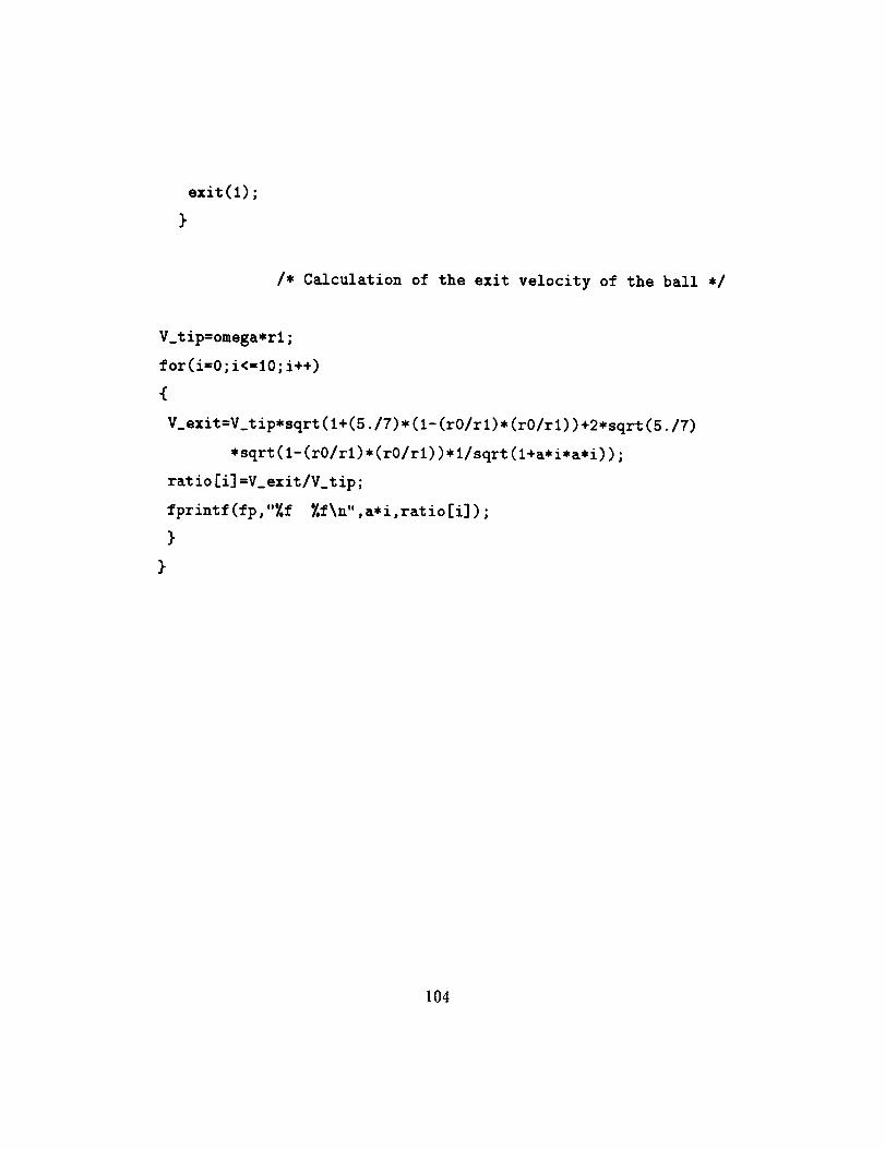
exit(l);

}

/* Calculation of the exit velocity of the ball */

V_tip=omega*rl;

for(i=O;i<=lO;i++)

{

V_exit=V_tip*sqrt(l+(5./?)*(1-(rO/rl)*(rO/rl))+2,sqrt(5./7)

*sqrt(1-(rO/rl)*(rO/rl))*I/sqrt(l+a,i,a,i));

ratio [i]=V_exit/V_tip ;

fprintf (fp, "%f %f\n", a,i, rat io [i]) ;

}

104

/* ROLLSKIDW.C */

/* THIS IS AN ANALYSIS OF THE SLIDING TENDENCY

OF THE BALL ON THE TRACK AS A FUNCTION OF

THE ANGULAR VELOCITY OF THE ROTOR */

#include "stdio.h"

#include <math.h>

main()

{

FILE *fp;

float r1=10e-2; /* radius of the rotor */

float omega; /* rotor angular speed (in radians per second) */

float omegaO=lO00.O;

/* track shape constant */

/* rotor tip speed (in meters per second) */

float a;

float V_tip;

float KO;

float K;

float t=O.5e-3;

/* constant appearing in the equations of motion */

/* time at which ball reaches the edge

of the track */

float th;

float ratio1[25] ;/* required coefficient of friction */

float ratio2[25] ;

float ratio3[25] ;

float ratio4[25] ;

int i;

105

/_ Opening of a file for the data */

if ((fp=f open ("rollskidv. dat", "w") )--=NULL)

{

printf("cannot open file\n") ;

exit(1);

}

/* Calculations and writing of the data */

V_tip=omega*rl;

a=0.5;

for(i=l;i<=20;i++)

(

omega=omegaO#i;

KO=5./(7*(l+I/(a_a)));

K=omega*sqrt(KO);

th=tanh(K*t);

ratiol[i]=2*a*sqrt(1+a*a)/(5*(1+th*th)+2*sqrt(55*(l+a*a))*th);

}

a=l.;

for(±=l;i<=20;i++)

{

omega=omegaO*i;

KO=5./(7*(l+l/(_*a)));

K=omega*sq_c(KO);

th=ta_h(K*t);

106

rat io2 [i] -2,a*sqrt (1+a,a) / (5* (l+th*th) +2*sqrt (35* (l+a*a)) *th) ;

)

a=3. ;

f or (i=l ;i<=20; i++)

{

omegaffiomegaO* i ;

KO=5. / (7* (1+1/(a,a) ) ) ;

K=omega*sqrt (KO) ;

th=t anh (K,t) ;

rat io3 [i] =2*a*sqrt (l+a*a) / (5, (i +th*th) +2*sqrt (35, (l+a*a)) *th) ;

}

a=10. ;

for (i=1; ±<=20; i++)

{

omega=omegaO* i ;

KO=5. / (7* (I+I/(a,a) )) ;

Kfomega*sqrt (KO) ;

th=tanh (K,t) ;

rat io4 [i] =2*a*sqrt (l+a*a) / (5* (l+th*th) +2*sqrt (35* (l+a*a)) *th) ;

fprintf(fp,"_.f _.f _.f Y.f 7.f\n",omega,ratiol[i] ,ratio2[i],

ratio3 [i], rat io4 [i] ) ;

}

107

/* ROLLSKIDA.C */

/* THIS IS AN ANALYSIS OF THE SLIDING TENDENCY

0F THE BALL 0N THE TRACK AS A FUNCTION OF

THE TRACK SHAPE CONSTANT */

#include "stdio.h"

#include <math.h>

main()

{

FILE *fp;

float rl=lOe-2;

float omega=tOe+3;

float a;

float aO=0.5;

float V_tip=omega*rl;

float ratio[25];

int i;

/* radius of the rotor */

/* angular velocity of the rotor */

/* track shape constant */

/* required coefficient of friction */

/* Opening of a file for the data */

if ((fp=f open ("rollskida. dat ", "w") )==NULL)

{

printf("cannot open file\n") ;

exit (1) ;

}

108

/* Calculations and writing of the data */

for (i,:O;i<=20; i÷+)

a_aO* i ;

ratio [i] =2*a*sqrt (1+a,a)/5 ;

fprintf (fp, "_,f _,f\n", a, ratio [i]) ;

109

/* KIN&DYN.C */

/* KINEMATICS AND DYNAMICS OF THE PRIMARY LAUNCHER,

THE BELAY, AND THE PROJECTILES. */

#include "stdio.h"

#include <math.h>

main()

{

FILE *fpl;

FILE *fp2;

/* DEFINITION OF THE PARAMETERS OF THE SYSTEM

(All distances are in meters and masses in kilograms) */

float rO=le-2;

float rl=lOe-2;

float i=0.5e-2;

float M=IO;

float m=4e-3;

float omega=lOe+3;

float a-l;

float MU_avai=0.93;

float a_max;

/* distance from the center of the rotor to

the beginning of the track */

/* radius of the rotor */

/* radius of the ball */

/* mass of the rotor */

/* mass of the ball */

/* rotor angular speed (in radians per second) */

/* track shape constant */

/* available coefficient of friction; in this case,

"stainless steel-stainless steel" */

/* maximum track shape constant allowed to

avoid skidding */

110

float MU_req; /* maximum coefficient of friction required

to avoid skidding _/

float epsilon=m/M; /* mass ratio */

float pi=3.141592654;

float T=2*pi/omega; /* rotor period of rotation (in seconds) */

float V_tip=omega*rl;/* rotor tip speed (in meters per second) */

float V_exit; /* exit velocity of the balls from the

primary launcher */

float KO=5./(7*(l+l/(a*a)));

float K; /* constant appearing in the equations

of motion */

int n=20; /* number of balls to be launched */

float t_exit[25]; /* t_exit[n]=time at which the nth ball

flies off the launcher */

float t_release[25]; /* t_release [n] =time at which the nth ball

is released near the center of the launcher */

float t_brt; /* time it takes the ball to roll on the

track From rO to rl */

float V_relay[25]; /* V_relay[n]=relay linear velocity just as

the nth ball leaves the relay heading back

toward the launcher */

float t_catch[25]; /* t_catch[n]=time at which the nth ball is

caught on the track of the relay _/

float zeta_c[25]; /* zeta_c[n]=angular position of the nth ball on

the track at catching time */

float tg;

float r_c; /* r_c=radial position of the ball on the track

111

float rdot_c;

float U;

int k;

int i;

float t_flight ;

float d_min;

float d;

float Del ;

float X1 ;

float X2 ;

float X;

float t ;

float t_brtup[25] ;

float t_exrel[25] ;

float X_relay[25] ;

float X_ball[25] ;

V_relay [0]=0. ;

K=omega*sqrt (KO) ;

at catching time */

/* rdot_c-d(r_c)/dt ,/

/* rotational speed of the ball (at the tip) */

/* time of flight of ball between the launcher

and the relay */

/* minimal initial separation between

the launcher and the relay */

/* actual initial separation */

/* t_brtup[n]=time for the nth ball to roll up

the track and reach the center of the relay

when starting at the impact point */

/* t_exrel[n]=time at which the nth ball

exits the relay and travels back to the

primary launcher */

/* X_relay[n]=position of the relay when it

is about to catch the nth ball */

/* X_ball[n]=position of the ball at

catching time */

/* relay initial velocity */

112

/* ROLL VERSUS SKID ANALYSIS */

a_max=sqrt((sqrt(1+25_MU_avai_MU_avai)-l)/2);

MUreq=2*a*sqrt(1÷a*a)/5;

if(MUavai>MU_req)

{

printf("Ball will roll nicely on track. Your choice of system

parameters is fine.You could choose 'a _ as high as Zf

if you wanted to).\n",a_max);

else

{

printf("Ball will skid on track. Choose another pair

of materials to change the value of MU_avai or,

simply choose a smaller value for 'a'. The maximal

acceptable value for 'a' is _f\n",a_max);

exit () ;

)

/* EXIT VELOCITY OF THE BALLS FROM THE PRIMARY LAUNCHER */

printf("The rotor tip speed is equal to Zf mls. \n",V_tip);

V_exit=V_tip*sqrt(l+(S.17)*(l-(rOlrl)*(rOlrl))÷

2*sqrt(S./7)*sqrt(l-(rO/rl)*(rOlrl))*llsqrt(l+a*a));

printf("The speed of the ball when it flies off the track of the

primary launcher is equal to Zf mls. \n",V_exit);

113

/* FDRWARD LAUNCH (PRIMARY LAUNCHER --- RELAY) */

/* Computation of the time it takes the ball to reach

the edge of the track (distance rl) when released

near the center at a distance rO */

t_brt=(1./K)*log(rl/r0+sqrt((rl/rO)*(rl/r0)-1));

printf("The time it takes the ball to reach the edge of the

track, when released near the center of the rotor

is texit[1]-trelease[1] = _f s.\n",t_brt);

/* Computation of the time at which the Ist ball exits

the launcher */

k=O;

labell:t_exit[1]=(1./omega)*(atan((-I/a)-(V_tip/(K*sqrt((rl*rl)-

(rO*r0)))))-(1./a)*log(rl/r0)+k*pi);

while(t_exit[l]<tbrt)

k=k+2;

goto labell;

}

/* Computation of the time at which the ist ball

is released near the center of the launcher */

114

t_release [i] =t_exi% [1] -t_brt ;

/* Times at which the ith ball is released and

exits the launcher, assuming we are launching

one ball every 2 revolutions of the rotor */

for (i=l; i<=n; i÷+)

{

t_exit [i] =t_exit [I] +2* (i-I) *T;

t_release [i] =t_release [I] +2* (i-I) *T;

}

/* RELAY VELOCITY AFTER THE LAUNCH DF THE ith ball */

for(i=l;i<=n;i++)

{

V_relay [i] =V_relay [i- i] +2* (eps ilon/(1+epsilon) )* (V_exit-V_relay [i- 1] ) ;

}

/* DETERMINATION OF THE CATCHING POSITION AND TIME */

/* Catching position and time for the 1st ball */

U=sqrt(5./7)*omega*sqrt((rl*rl)-(r0*r0));

tg=sqrt(pow((V_exit-V_relay[0])/U,2)*(l+i/pow(a,2))-l);

zeta_c[1]=-(1/a)*log((-U*(l-a*tg))/(omega*r0*sqrt(l+pow(a,2))));

k=l;

115

label2 :t_catch [I]=(I/omega) * (atan (tg)-zet a_c [I] +k*pi) ;

while(t_catch [I]<=t_exit [I])

{

k=k+2 ;

goto label2;

)

/* Initial separation between the primary launcher

and the relay */

t_flight=t_catch [I]-t_exit [I] ;

d_min=V_exit*t_flight ;

printf("The minimal initial separation is Zf m. \n",d_min);

printf("It is better to start with a distance of at least

500 m, which means that the ball is caught several

revolutions later than this value of t_catch[1]

determined above. Let us add then to t_catch[1],

2k(pi)/omega until we reach our goal of 500 m.\n");

k=l ;

label3 :t_catch [1]= (1/omega)* (atan (tg)-zeta_c [1]+k*pi) ;

t_flight=t_catch [i]-t_exit [1] ;

d=V_exit*t_flight ;

while(d<500)

k=k+2;

goto label3 ;

116

printf("The initial separation is now set to _.fm.\n",d);

/* Catching position and time for the ith ball */

for (i=2; i<=n; i++)

{

tg=sqrt (pow ((V_exit-V_relay [i-l] )/U, 2) *(I+I/pow (a,2) )-I) ;

if(tg>1. )

{

zet a_c [i]=- (l/a) *log ((-U* (l-a*tg) )/(omega*r0

•sqrt (l+pow(a, 2) ))) ;

label4 :t_catch [i]=(1/omega) *(atan (tg)-zet a_c [i]+k*pi) ;

while (t_catch[i] <= (t_exit [i]+t_flight) )

<

kfk+2;

goto label4;

}

}

else

{

printf("The maximum number of balls that can be caught

is _.d\n",i-1) ;

exit () ;

/* BALL ON RELAY */

117

/* 1st phase: from impact point to center of relay */

for(i=l;i<=n;i++)

{

r_c=rO*exp(-a*zeta_c[i]);

rdot_c=(a*r_c*omega-a*sqrt(pow(V_exit,2)*(l+a*a)-

pow(a*r_c*omega,2)))l(l+a*a);

Del=(pow((rdot_c/K),2))*(pow((rdot_c/Z),2)-(r_c*r_c-rO*rO));

Xl=((-r_c*rO)-sqrt(Del))/((pow((rdot_c/K),2))-(r_c*r_c));

X2=((-r_c*rO)+sqrt(Del))l((pow((rdot_clK),2))-(r_c*r_c));

if(Xl>O)

{

if(Xl<=lO)

{

X=X1;

}

else

{

X=X2 ;

}

}

else

{

X=X2;

}

118

t_brtup [i] = (1./K)* (log (X+sqrt ( (X,X)- 1.0)) ) ;

}

/* 2nd phase: from center of relay to edge of track */

for(i=l;i<=n;i++)

k=l;

label5:t_exrel[i]=(1./omega)*(atan((-1/a)-(V_tip/(K*sqrt((rl*rl)

-(rO*rO)))))-(1./a)*log(rl/rO)+k*pi);

t=t_cat ch [i] +t_brtup [i] +t_brt ;

while (t_exrel [i] <t)

{

k=k+2;

goto labelS;

}

}

/* POSITION OF THE RELAY */

X_relay [i]=d;

for (i=2; i<=n; i++)

{

X_relay [i]=X_relay [i-l] +(V_relay [i- i]* (t_catch [i]-t_exrel [i- i]));

}

/* POSITION OF THE ITH BALL AT THE TIME OF CATCH */

119

X_ball [I] =d;

for (i=2 ;i<--n; i++)

{

X_ball [i] =V_exit* (t_catch [i] -t_exit [i] ) ;

}

/* OPENING OF FILES FOR THE DATA */

if ( (fp l=f open ("time. dat", "w" ))==NULL)

{

printf("cannot open file\n") ;

exit (1) ;

if ((fp2=f open ("posit ion. dat", "w" ))==NULL)

{

printf("cannot open filekn") ;

exit (1) ;

}

/* WRITING THE DATA */

for (i=l ;i<--n ;i++)

{

fprintf(fp1,"_.f _.f Y.f Y.f _.fkn",t_release[i] ,t_exit[i],

t_catch[i] ,t_brtup [i] ,t_exrel[i] ) ;

fprintf(fp2,"_.f _.f _.f Y.f \n" ,zeta_c [i] ,V_relay[i],

120

X_relay [i],X_ball [i]);

121

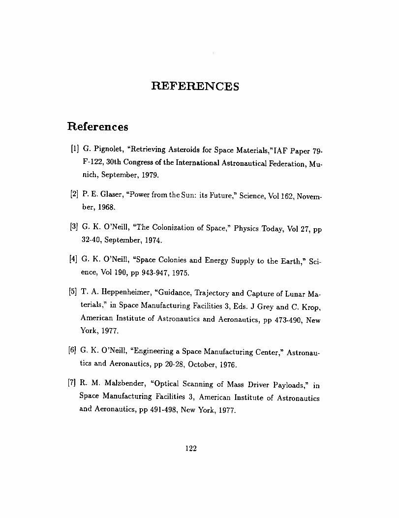
REFERENCES

References

[1] G. Pignolet, "Retrieving Asteroids for Space Materials,"IAF Paper 79-

F-122, 30th Congress of the International Astronautical Federation, Mu-

nich, September, 1979.

[2] P. E. Glaser, "Power from the Sun: its Future," Science, Vol 162, Novem-

ber, 1968.

[3] G. K. O'Neill, "The Colonization of Space," Physics Today, Vol 27, pp

32-40, September, 1974.

[4] G. K. O'Neill, "Space Colonies and Energy Supply to the Earth," Sci-

ence, Vol 190, pp 943-947, 1975.

[5] T. A. Heppenheimer, "Guidance, Trajectory and Capture of Lunar Ma-

terials," in Space Manufacturing Facilities 3, Eds. J Grey and C. Krop,

American Institute of Astronautics and Aeronautics, pp 473-490, New

York, 1977.

[6] G. K. O'Neill, "Engineering a Space Manufacturing Center," Astronau-

tics and Aeronautics, pp 20-28, October, 1976.

[7] R. M. Malzbender, "Optical Scanning of Mass Driver Payloads," in

Space Manufacturing Facilities 3, American Institute of Astronautics

and Aeronautics, pp 491-498, New York, 1977.

122

[8] J. Pearson, "Law-Cost Launch System and Orbital Fuel Depot," IAF

Paper 86-128, 37th Congress of the International Astronautical Federa-

tion, Innsbruck, Austria, October, 1986.

[9] M. W. Hunter, "Transportation: Options and High-Payoff Choices,"

Space Solar Power Rev., Vol 4, pp 99-117, 1983.

[10] L. W. Jones and D. K. Keefer, "NASA's Laser propulsion Project,"

Astronautics and Aeronautics, Vol 20, No 9, pp 66-73, 1982.

[11] J. Pearson, "The Orbital Tower: a Spacecraft Launcher Using the

Earth's Rotational Energy," Acta Astronautica, Vol 2, pp 785-799, 1975.

[12] Y. Artsutanov, "V Kosmos Bez Raket," Znanije-Sila, Vol 7, pp 25, 1969.

[13] H. Moravec, "A Non-Synchronous Rolling Skyhook," Journal of astro-

nautical science, Vol 25, pp 307-322, 1978.

[14] P. M. Birch, "Orbital Ring Systems and Jacob's Ladders," Journal of

the British Interplanetary Society, Vol 35, pp 475-497, 1982.

[15] K. Lofstrom, "The Launch Loop - A Low cost Earth-to-High Orbit

Launch System," AIAA Paper 85-1368, 1985.

[16] K. E. Drexel, "High Performance Solar Sails and Related Reflecting

Devices," AIAA Paper 79-1418, 4th Princeton/AIAA Conf. on Space

Manufacturing Facilities, May, 1979.

[17] G. Marx, Nature, Vol 211, pp 22, 1966.

[18] C. E. Singer, "Spaceborne Centrifugal Relays for Spacecraft Propulsion

and Rapid Launch of High-Velocity Projectiles," Contract NASA NAG3-

1037 Proposal, March, 1988.

123

[19] C. E. Singer, "Interstellar Propulsion Using a Pellet Stream for Momen-

tum Transfer," Journal of the British Interplanetary Society, Vol 33, pp

107-115, March 1980.

[20] C. E. Singer, "Questions Conserning Pellet-Stream Propulsion," Journal

of the British Interplanetary Society, Vol 34, pp 117-119, 1981.

[21] F. Chilton, B. Hibbs, H. Kolm, G. K. O'Neill, and K. Phillips, "Mass

Driver Applications in Space-based Manufacturing from Non-terrestrial

Materials," in Prog. in Astronautics and Aeronautics, Eds. G. K. O'Neill

and B. O'Leary, American Institute of Aeronautics and Astronautics,

Vol 57, pp 63-94, New York, 1977.

[22] H. Kolm, K. Fine, P. Mongeau, and F. Wilhams, "Electromagnetic

Propulsion Alternative," Paper AIAA-79-1418, 4th Princeton/AIAA

Conf. on Space Manufacturing Facilities, 14-17 May, 1979.

[23] F. S. Felber, "Centrifugal Projectile Launcher," IEEE Trans. Magnetics,

Vol MAG-18, No 1, pp 209-212, January, 1982.

[24] C. E. Singer, and F. R. Singer, "Centrifugal Relays for Spacecraft

Propulsion," Journal of the British Interplanetary Society, Vol 44, pp

127-134, 1991.

[25] K. Fine, "Basic Coaxial Mass Driver Construction and Testing,"

Progress Report, Department of Aeronautics and Astronautics, MIT,

March, 1979.

[26] S. Sudo, T. Baba, K. Kakubari, and K. Uo, "Pellet Guidance System

for Flexible Density Profile Control and its Operation Characteristics,"

Fusion Technology, Vol 14, pp 1334-1342, November, 1988.

124

[27] S. K. Coombs, S. L. Milora, C. A. Foster, D.D. SchuresKo, and J. T.

Hogan, "Development of Hydrogen Pellet Injectors at ORNL," Nucl.

Tech./Fusion, Vol 4, pp 666-669, September, 1983.

[28] B. P. Von Herzen, "Light pressure and Solar Wind Perturbations to

Payload Trajectories," in Space Manufacturing Facilities 3, American

Institute of Astronautics and Aeronautics, pp 499-501, New York, 1977.

[29] S. T. Pang, "Centrifugal Relay Design: Pellet Kinematics and Roll/Slide

Analysis," NASA Progress Report, October, 1990.

[30] D. A. Levinson and D. B. Schaechter, "Autolev', 1988.

[31] J. B. Ditman, "Centrifugal Relay Design; Catching and Particle Simu-

lation," NASA Progress Report, November, 1990.

[32] D. Leo, "Preliminary Design of Centrifugal Relays," NASA Progress

Report, May, 1990.

[33] R. D. Johnson and C. Holbrow, "Rotary Pellet Launcher," NASA SP-

413, pp 130-132, 1975.

[34] S. V. Kulkarni, "Flywheel Rotor and Containment Technology Develop-

ment of the U.S. Department of Energy," University of California Report

UCRL-84713, August, 1980.

125

OF POOR QUAt ;TY