rounding-based moves for semi-metric labeling
TRANSCRIPT

HAL Id: hal-01577719https://hal.inria.fr/hal-01577719
Submitted on 27 Aug 2017
HAL is a multi-disciplinary open accessarchive for the deposit and dissemination of sci-entific research documents, whether they are pub-lished or not. The documents may come fromteaching and research institutions in France orabroad, or from public or private research centers.
L’archive ouverte pluridisciplinaire HAL, estdestinée au dépôt et à la diffusion de documentsscientifiques de niveau recherche, publiés ou non,émanant des établissements d’enseignement et derecherche français ou étrangers, des laboratoirespublics ou privés.
Rounding-based Moves for Semi-Metric LabelingM. Pawan Kumar, Puneet K. Dokania
To cite this version:M. Pawan Kumar, Puneet K. Dokania. Rounding-based Moves for Semi-Metric Labeling . Journal ofMachine Learning Research, Microtome Publishing, 2016, 17, pp.1 - 42. �hal-01577719�
Journal of Machine Learning Research 17 (2016) 1-42 Submitted 10/14; Revised 12/15; Published 4/16
Rounding-based Moves for Semi-Metric Labeling
M. Pawan Kumar [email protected]
Department of Engineering ScienceUniversity of OxfordParks Road OX1 3PJUnited Kingdom
Puneet K. Dokania [email protected]
Center for Visual ComputingCentraleSupelec92295 Chatenay-MalabryFrance
Editor: Jeff Bilmes
AbstractSemi-metric labeling is a special case of energy minimization for pairwise Markov random fields.The energy function consists of arbitrary unary potentials, and pairwise potentials that are propor-tional to a given semi-metric distance function over the label set. Popular methods for solvingsemi-metric labeling include (i) move-making algorithms, which iteratively solve a minimum st-cutproblem; and (ii) the linear programming (LP) relaxation based approach. In order to convert the frac-tional solution of the LP relaxation to an integer solution, several randomized rounding procedureshave been developed in the literature. We consider a large class of parallel rounding procedures,and design move-making algorithms that closely mimic them. We prove that the multiplicativebound of a move-making algorithm exactly matches the approximation factor of the correspondingrounding procedure for any arbitrary distance function. Our analysis includes all known results formove-making algorithms as special cases.
Keywords: semi-metric labeling, move-making algorithms, linear programming relaxation, multi-plicative bounds
1. Introduction
A Markov random field (MRF) is a graph whose vertices are random variables, and whose edgesspecify a neighborhood over the random variables. Each random variable can be assigned a valuefrom a set of labels, resulting in a labeling of the MRF. The putative labelings of an MRF arequantitatively distinguished from each other by an energy function, which is the sum of potentialfunctions that depend on the cliques of the graph. An important optimization problem associate withthe MRF framework is energy minimization, that is, finding a labeling with the minimum energy.
Semi-metric labeling is a special case of energy minimization, which models several usefullow-level vision tasks (Boykov et al., 1998, 1999; Szeliski et al., 2008). It is characterized by a finite,discrete label set and a semi-metric distance function over the labels. The energy function in semi-
c©2016 M. Pawan Kumar and Puneet Dokania.

KUMAR AND DOKANIA
metric labeling consists of arbitrary unary potentials and pairwise potentials that are proportionalto the distance between the labels assigned to them. The problem is known to be NP-hard (Veksler,1999). Two popular approaches for semi-metric labeling are: (i) move-making algorithms (Boykovet al., 1999; Gupta and Tardos, 2000; Kumar and Koller, 2009; Kumar and Torr, 2008; Veksler,2007), which iteratively improve the labeling by solving a minimum st-cut problem; and (ii) linearprogramming (LP) relaxation (Chekuri et al., 2001; Koster et al., 1998; Schlesinger, 1976; Wainwrightet al., 2005), which is obtained by dropping the integral constraints in the corresponding integerprogramming formulation. Move-making algorithms are very efficient due to the availability of fastminimum st-cut solvers (Boykov and Kolmogorov, 2004) and are very popular in the computer visioncommunity. In contrast, the LP relaxation is significantly slower, despite the development of severalspecialized solvers (Globerson and Jaakkola, 2007; Hazan and Shashua, 2008; Kolmogorov, 2006;Komodakis et al., 2007; Ravikumar et al., 2008; Tarlow et al., 2011; Wainwright et al., 2005; Weisset al., 2007; Werner, 2007, 2010). However, when used in conjunction with randomized roundingalgorithms, the LP relaxation provides the best known polynomial-time theoretical guarantees forsemi-metric labeling (Archer et al., 2004; Chekuri et al., 2001; Kleinberg and Tardos, 1999).
At first sight, the difference between move-making algorithms and the LP relaxation appearsto be the standard accuracy vs. speed trade-off. However, we prove that, for any arbitrary semi-metric distance function, it is possible to design move-making algorithms that match the theoreticalguarantees of a large class of randomized rounding procedures, which we call parallel rounding.Our proofs are constructive, which allows us to test the rounding-based move-making algorithmsempirically. Our experimental results confirm that rounding-based moves provide similar accuracyto the LP relaxation while being significantly faster.
2. Related Work
As our work is concerned with only semi-metric labeling, we will focus on the related work forthis special case of energy minimization. For a more general survey, we refer the reader to (Wanget al., 2013), and for a thorough empirical comparison of the various algorithms we refer the readerto (Kappes et al., 2015; Szeliski et al., 2008).
The earliest known theoretical guarantee of a move-making algorithm was provided by Veksler(1999), who presented an analysis of the popular expansion move-making algorithm. The analysisshowed that the expansion algorithm and the parallel rounding procedure of Kleinberg and Tardos(1999) provide matching guarantees for the uniform distance function. Komodakis et al. (2008)also proposed a move-making algorithm based on the primal-dual scheme of optimizing the LP
relaxation. The resulting algorithm is similar to the expansion algorithm in terms of its theoreticalguarantees, but provides a principled formulation for improving its efficiency in dynamic settings.Despite the existing analysis of expansion-like algorithms, parallel rounding procedures (Chekuriet al., 2001; Kleinberg and Tardos, 1999) are known to perform better for several distance functions ofinterest such as the truncated linear distance, the truncated quadratic distance, and the hierarchicallywell-separated tree (HST) metric.
Kumar and Torr (2008) proposed the range expansion move-making algorithm that matches theguarantees of the rounding procedure of Chekuri et al. (2001) for the truncated linear and quadraticdistance. Kumar and Koller (2009) proposed a hierarchical move-making algorithm that matches theguarantees of the rounding procedure of Kleinberg and Tardos (1999) for the HST metric. However,their analysis is restricted to special cases of semi-metric labeling, whereas our work does not make
2

ROUNDING-BASED MOVES FOR SEMI-METRIC LABELING
any assumptions on the form of the semi-metric distance function. We note that, recently, a moregeneral algorithm has also been proposed for non-convex priors (Ajanthan et al., 2014). However,this generalized algorithm does not provide any strong theoretical gurantees on the quality of thesolution, which is the key focus of our work.
While our analysis focuses on parallel rounding, it is also worth noting that Archer et al. (2004)have proposed a serial rounding procedure for metric labeling (which is a special case of semi-metriclabeling where the distance function also satisfies the triangular inequality property). The theoreticalguarantee of serial rounding depends on the tree decomposibility of a distance function. Given anMRF with n random variables, the tree decomposibility for any metric distance function is guaranteedto be less than or equal to O(log n). This worst-case theoretical guarantee of O(log n) over all metricdistance functions can be matched by a mixture-of-tree algorithm that can be derived form the workof Andrew et al. (2011). Specifically, Andrew et al. (2011) describe an approximate algorithm forcapacitated metric labeling that builds on the cut-based decomposition method of Racke (2008).Ignoring the capacity constraints, which are not present in the standard metric labeling problem,results in an approximation of the original MRF using an O(m log n) mixture of tree-structured MRFs.Here, m is the number of edges in the MRF, and n is the number of random variables. Solving themetric labeling problem over each tree-structured MRF optimally using belief propagation (Pearl,1998), and choosing the best labeling in terms of the original problem, provides the O(log n)guarantee. We refer the reader to (Andrew et al., 2011) for details.
Note that while the mixture-of-tree algorithm provides matching worst-case guarantees to serialrounding, it does not provide a matching guarantee for a given distance function. In other words,the guarantee of the mixture-of-tree algorithm does not depend on the tree decomposibility of thedistance function. The existence or the impossibility of a matching combinatorial algorithm for serialrounding remains an open question.
3. Our Contributions
Our paper can be thought of as a generalization of (Kumar and Koller, 2009; Kumar and Torr, 2008;Veksler, 1999). Indeed, the move-making algorithms proposed in this paper are simple extensions ofthe expansion, the range expansion and the hierarchical move-making algorithms. The novelty of ourwork lies in our analysis, which improves on the state of the art in two significant aspects. First, we donot place any assumptions on the form of the distance function except that it is a semi-metric distance.This is in contrast to previous works that only focus on special cases such as the uniform metric, thetruncated convex models or the HST metric. Second, we show that the matching guarantees providedby our move-making algorithms and the parallel rounding procedures are tight, that is, they cannotbe improved through a more careful analysis.
A preliminary version of this article has appeared as (Kumar, 2014). There are two significantdifferences between the preliminary version and the current paper. First, we provide detailed proofsof all the theorems, which were omitted from the preliminary version due to a lack of space. Second,we provide an experimental comparison of the rounding-based move-making algorithms with thestate of the art methods for semi-metric labeling, including those that are directly related to theLP relaxation such as TRW-S (Kolmogorov, 2006), and those that are indirectly related to the LP
relaxation such as (Andrew et al., 2011).Finally, we note that since the publication of the preliminary version, we have also extended
rounding-based move-making algorithms to special cases of high-order potentials. This includes the
3
KUMAR AND DOKANIA
interval move-making algorithm for truncated max-of-convex potentials (Pansari and Kumar, 2015)and the hierarchical move-making algorithm for parsimonious labeling (Dokania and Kumar, 2015).
4. Preliminaries
4.1 Semi-metric Labeling
The problem of semi-metric labeling is defined over an undirected graph G = (X,E). The verticesX = {X1, X2, · · · , Xn} are random variables, and the edges E specify a neighborhood relationshipover the random variables. Each random variable can be assigned a value from the label setL = {l1, l2, · · · , lh}. We assume that we are also provided with a semi-metric distance functiond : L× L→ R+ over the labels. Recall that a semi-metric distance function satisfies the followingproperties: d(li, lj) ≥ 0 for all li, lj ∈ L, and d(li, lj) = 0 if and only if i = j. Furthermore,a distance function is said to be metric if, in addition to the above condition, it also satisfies thetriangular inequality, that is, d(li, lj) + d(lj , lk) ≥ d(li, lk) for all li, lj , lk ∈ L.
We refer to an assignment of values to all the random variables as a labeling. In other words, alabeling is a vector x ∈ Ln, which specifies the label xa assigned to each random variable Xa. Thehn different labelings are quantitatively distinguished from each other by an energy function Q(x),which is defined as follows:
Q(x) =∑
Xa∈Xθa(xa) +
∑(Xa,Xb)∈E
wabd(xa, xb).
Here, the unary potentials θa(·) are arbitrary, and the edge weights wab are non-negative. Semi-metriclabeling requires us to find a labeling with the minimum energy. It is known to be NP-hard.
4.2 Multiplicative Bound
As semi-metric labeling plays a central role in low-level vision, several approximate algorithmshave been proposed in the literature. A common theoretical measure of accuracy for an approximatealgorithm is the multiplicative bound. In this work, we are interested in the multiplicative bound of analgorithm with respect to a distance function. Formally, given a distance function d, the multiplicativebound of an algorithm is said to be B if the following condition is satisfied for all possible values ofunary potentials θa(·) and non-negative edge weights wab:∑
Xa∈Xθa(xa) +
∑(Xa,Xb)∈E
wabd(xa, xb) ≤∑
Xa∈Xθa(x
∗a) +B
∑(Xa,Xb)∈E
wabd(x∗a, x∗b). (1)
Here, x is the labeling estimated by the algorithm for the given values of unary potentials and edgeweights, and x∗ is an optimal labeling. Multiplicative bounds are greater than or equal to 1, and areinvariant to reparameterizations of the unary potentials. A multiplicative bound B is said to be tightif the above inequality holds as an equality for some value of unary potentials and edge weights.
4.3 Linear Programming Relaxation
An overcomplete representation of a labeling can be specified using the following variables: (i) unaryvariables ya(i) ∈ {0, 1} for all Xa ∈ X and li ∈ L such that ya(i) = 1 if and only if Xa is assignedthe label li; and (ii) pairwise variables yab(i, j) ∈ {0, 1} for all (Xa, Xb) ∈ E and li, lj ∈ L such
4

ROUNDING-BASED MOVES FOR SEMI-METRIC LABELING
that yab(i, j) = 1 if and only if Xa and Xb are assigned labels li and lj respectively. This allows usto formulate semi-metric labeling as follows:
miny
∑Xa∈X
∑li∈L
θa(li)ya(i) +∑
(Xa,Xb)∈E
∑li,lj∈L
wabd(li, lj)yab(i, j),
s.t.∑li∈L
ya(i) = 1, ∀Xa ∈ X,
∑lj∈L
yab(i, j) = ya(i), ∀(Xa, Xb) ∈ E, li ∈ L,
∑li∈L
yab(i, j) = yb(j), ∀(Xa, Xb) ∈ E, lj ∈ L,
ya(i) ∈ {0, 1}, yab(i, j) ∈ {0, 1}, ∀Xa ∈ X, (Xa, Xb) ∈ E, li, lj ∈ L.
The first set of constraints ensures that each random variables is assigned exactly one label. Thesecond and third sets of constraints ensure that, for binary optimization variables, yab(i, j) =ya(i)yb(j). By relaxing the final set of constraints such that the optimization variables can take anyvalue between 0 and 1 inclusive, we obtain a linear program (LP). The computational complexity ofsolving the LP relaxation is polynomial in the size of the problem.
4.4 Rounding Procedure
In order to prove theoretical guarantees of the LP relaxation, it is common to use a rounding procedurethat can covert a feasible fractional solution y of the LP relaxation to a feasible integer solution yof the integer linear program. Several rounding procedures have been proposed in the literature.In this work, we focus on the randomized parallel rounding procedures proposed by Chekuri et al.(2001) and Kleinberg and Tardos (1999). These procedures have the property that, given a fractionalsolution y, the probability of assigning a label li ∈ L to a random variable Xa ∈ X is equal to ya(i),that is,
Pr(ya(i) = 1) = ya(i). (2)
We will describe the various rounding procedures in detail in Sections 5-7. For now, we would liketo note that our reason for focusing on the parallel rounding of Chekuri et al. (2001) and Kleinbergand Tardos (1999) is that they provide the best known polynomial-time theoretical guarantees forsemi-metric labeling. Specifically, we are interested in their approximation factor, which is definednext.
4.5 Approximation Factor
Given a distance function d, the approximation factor for a rounding procedure is said to be F if thefollowing condition is satisfied for all feasible fractional solutions y:
E
∑li,lj∈L
d(li, lj)ya(i)yb(j)
≤ F ∑li,lj∈L
d(li, lj)yab(i, j). (3)
Here, y refers to the integer solution, and the expectation is taken with respect to the randomizedrounding procedure applied to the feasible solution y.
5

KUMAR AND DOKANIA
Given a rounding procedure with an approximation factor of F , an optimal fractional solution y∗
of the LP relaxation can be rounded to a labeling y that satisfies the following condition:
E
∑Xa∈X
∑li∈L
θa(li)ya(i) +∑
(Xa,Xb)∈E
∑li,lj∈L
wabd(li, lj)ya(i)yb(j)
≤
∑Xa∈X
∑li∈L
θa(li)y∗a(i) + F
∑(Xa,Xb)∈E
∑li,lj∈L
wabd(li, lj)y∗ab(i, j).
The above inequality follows directly from properties (2) and (3). Similar to multiplicative bounds,approximation factors are always greater than or equal to 1, and are invariant to reparameterizationsof the unary potentials. An approximation factor F is said to be tight if the above inequality holds asan equality for some value of unary potentials and edge weights.
Approximation factors are closely linked to the integrality gap of the LP relaxation (roughlyspeaking, the ratio of the optimal value of the integer linear program to the optimal value of therelaxation), which in turn is related to the computational hardness of the semi-metric labelingproblem (Manokaran et al., 2008). However, establishing the integrality gap of the LP relaxationfor a given distance function is beyond the scope of this work. We are only interested in designingmove-making algorithms whose multiplicative bounds match the approximation factors of the parallelrounding procedures.
4.6 Submodular Energy Function
We will use the following important fact throughout this paper. Given an energy function definedusing arbitrary unary potentials, non-negative edge weights and a submodular distance function, anoptimal labeling can be computed in polynomial time by solving an equivalent minimum st-cutproblem (Flach and Schlesinger, 2006). Recall that a submodular distance function d′ over a labelset L = {l1, l2, · · · , lh} satisfies the following properties: (i) d′(li, lj) ≥ 0 for all li, lj ∈ L, andd′(li, lj) = 0 if and only if i = j; and (ii) d′(li, lj) + d′(li+1, lj+1) ≤ d′(li, lj+1) + d′(li+1, lj) forall li, lj ∈ L\{lh} (where \ refers to set difference).
5. Complete Rounding and Complete Move
We start with a simple rounding scheme, which we call complete rounding. While complete roundingis not very accurate, it would help illustrate the flavor of our results. We will subsequently considerits generalizations, which have been useful in obtaining the best-known approximation factors forvarious special cases of semi-metric labeling.
The complete rounding procedure consists of a single stage where we use the set of all unaryvariables to obtain a labeling (as opposed to other rounding procedures discussed subsequently).Algorithm 1 describes its main steps. Intuitively, it treats the value of the unary variable ya(i) as theprobability of assigning the label li to the random variable Xa. It obtains a labeling by sampling fromall the distributions ya = [ya(i), ∀li ∈ L] simultaneously using the same random number r ∈ [0, 1].
It can be shown that using a different random number to sample the distributions ya and yb oftwo neighboring random variables (Xa, Xb) ∈ E results in an infinite approximation factor. Forexample, let ya(i) = yb(i) = 1/h for all li ∈ L, where h is the number of labels. The pairwisevariables yab that minimize the energy function are yab(i, i) = 1/h and yab(i, j) = 0 when i 6= j.
6
ROUNDING-BASED MOVES FOR SEMI-METRIC LABELING
For the above feasible solution of the LP relaxation, the RHS of inequality (3) is 0 for any finite F ,while the LHS of inequality (3) is strictly greater than 0 if h > 1. However, we will shortly show thatusing the same random number r for all random variables provides a finite approximation factor.
Algorithm 1 The complete rounding procedure.input A feasible solution y of the LP relaxation.
1: Pick a real number r uniformly from [0, 1].2: for all Xa ∈ X do3: Define Ya(0) = 0 and Ya(i) =
∑ij=1 ya(j) for all li ∈ L.
4: Assign the label li ∈ L to the random variable Xa if Ya(i− 1) < r ≤ Ya(i).5: end for
We now turn our attention to designing a move-making algorithm whose multiplicative boundmatches the approximation factor of the complete rounding procedure. To this end, we modifythe range expansion algorithm proposed by Kumar and Torr (2008) for truncated convex pairwisepotentials to a general semi-metric distance function. Our method, which we refer to as the completemove-making algorithm, considers all putative labels of all random variables, and provides anapproximate solution in a single iteration. Algorithm 2 describes its two main steps. First, itcomputes a submodular overestimation of the given semi-metric distance function by solving thefollowing optimization problem:
d = argmind′
t (4)
s.t. d′(li, lj) ≤ td(li, lj), ∀li, lj ∈ L,
d′(li, lj) ≥ d(li, lj),∀li, lj ∈ L,
d′(li, lj) + d′(li+1, lj+1) ≤ d′(li, lj+1) + d′(li+1, lj), ∀li, lj ∈ L\{lh}.
The above problem minimizes the maximum ratio of the estimated distance to the original distanceover all pairs of labels, that is,
maxi 6=j
d′(li, lj)
d(li, lj).
We will refer to the optimal value of problem (4) as the submodular distortion of the distancefunction d. Second, it replaces the original distance function by the submodular overestimation andcomputes an approximate solution to the original semi-metric labeling problem by solving a singleminimum st-cut problem. Note that, unlike the range expansion algorithm (Kumar and Torr, 2008)that uses the readily available submodular overestimation of a truncated convex distance (namely,the corresponding convex distance function), our approach estimates the submodular overestimationvia the LP (4). Since the LP (4) can be solved for any arbitrary distance function, it makes completemove-making more generally applicable.
The following theorem establishes the theoretical guarantees of the complete move-makingalgorithm and the complete rounding procedure.
Theorem 1 The tight multiplicative bound of the complete move-making algorithm is equal to thesubmodular distortion of the distance function. Furthermore, the tight approximation factor of thecomplete rounding procedure is also equal to the submodular distortion of the distance function.
7

KUMAR AND DOKANIA
Algorithm 2 The complete move-making algorithm.input Unary potentials θa(·), edge weights wab, distance function d.
1: Compute a submodular overestimation of d by solving problem (4).2: Using the approach of Flach and Schlesinger (2006), solve the following problem via an
equivalent minimum st-cut problem:
x = argminx∈Ln
∑Xa∈X
θa(xa) +∑
(Xa,Xb)∈E
wabd(xa, xb).
The proof of Theorem 1 is given in Appendix A. The following corollary of the above theorem waspreviously stated by Chekuri et al. (2001) without a formal proof.
Corollary 2 The complete rounding procedure is tight for submodular distance functions, that is, itsapproximation factor is equal to 1.
In terms of computational complexities, complete move-making is significantly faster thansolving the LP relaxation. Specifically, given an MRF with n random variables and m edges, anda label set with h labels, the LP relaxation requires at least O(m3h3 log(m2h3)) time, since itconsists of O(mh2) optimization variables and O(mh) constraints. In contrast, complete move-making requires O(nmh3 log(m)) time, since the graph constructed using the method of Flach andSchlesinger (2006) consists of O(nh) nodes and O(mh2) arcs. Note that complete move-makingalso requires us to solve the linear program (4). However, since problem (4) is independent of theunary potentials and the edge weights, it only needs to be solved once beforehand in order to computethe approximate solution for any semi-metric labeling problem defined using the distance function d.
6. Interval Rounding and Interval Moves
Theorem 1 implies that the approximation factor of the complete rounding procedure is very largefor distance functions that are highly non-submodular. For example, consider the truncated lineardistance function defined as follows over a label set L = {l1, l2, · · · , lh}:
d(li, lj) = min{|i− j|,M}.
Here,M is a user specified parameter that determines the maximum distance. The tightest submodularoverestimation of the above distance function is the linear distance function, that is, d(li, lj) = |i− j|.This implies that the submodular distortion of the truncated linear metric is (h−1)/M , and therefore,the approximation factor for the complete rounding procedure is also (h− 1)/M . In order to avoidthis large approximation factor, Chekuri et al. (2001) proposed an interval rounding procedure, whichcaptures the intuition that it is beneficial to assign similar labels to as many random variables aspossible.
Algorithm 3 provides a description of interval rounding. The rounding procedure chooses aninterval of at most q consecutive labels (step 2). It generates a random number r (step 3), and uses itto attempt to assign labels to previously unlabeled random variables from the selected interval (steps4-7). It can be shown that the overall procedure converges in a polynomial number of iterationswith a probability of 1 (Chekuri et al., 2001). Note that if we fix q = h and z = 1, interval
8

ROUNDING-BASED MOVES FOR SEMI-METRIC LABELING
rounding becomes equivalent to complete rounding. However, the analyses of Chekuri et al. (2001)and Kleinberg and Tardos (1999) shows that other values of q provide better approximation factorsfor various special cases.
Algorithm 3 The interval rounding procedure.input A feasible solution y of the LP relaxation.
1: repeat2: Pick an integer z uniformly from [−q + 2, h]. Define an interval of labels I = {ls, · · · , le},
where s = max{z, 1} is the start index and e = min{z + q − 1, h} is the end index.3: Pick a real number r uniformly from [0, 1].4: for all Unlabeled random variables Xa do5: Define Ya(0) = 0 and Ya(i) =
∑s+i−1j=s ya(j) for all i ∈ {1, · · · , e− s+ 1}.
6: Assign the label ls+i−1 ∈ I to the Xa if Ya(i− 1) < r ≤ Ya(i).7: end for8: until All random variables have been assigned a label.
Our goal is to design a move-making algorithm whose multiplicative bound matches the ap-proximation factor of interval rounding for any choice of q. To this end, we propose the intervalmove-making algorithm that generalizes the range expansion algorithm (Kumar and Torr, 2008),originally proposed for truncated convex distances, to arbitrary distance functions. Algorithm 4provides its main steps. The central idea of the method is to improve a given labeling x by allowingeach random variable Xa to either retain its current label xa or to choose a new label from an intervalof consecutive labels. In more detail, let I = {ls, · · · , le} ⊆ L be an interval of labels of length atmost q (step 4). For the sake of simplicity, let us assume that xa /∈ I for any random variable Xa.We define Ia = I
⋃{xa} (step 5). For each pair of neighboring random variables (Xa, Xb) ∈ E,
we compute a submodular distance function dxa,xb: Ia × Ib → R+ by solving the following linear
program (step 6):
dxa,xb= argmin
d′t (5)
s.t. d′(li, lj) ≤ td(li, lj), ∀li ∈ Ia, lj ∈ Ib,
d′(li, lj) ≥ d(li, lj),∀li ∈ Ia, lj ∈ Ib,
d′(li, lj) + d′(li+1, lj+1) ≤ d′(li, lj+1) + d′(li+1, lj), ∀li, lj ∈ I\{le},d′(li, le) + d′(li+1, xb) ≤ d′(li, xb) + d′(li+1, le), ∀li ∈ I\{le},d′(le, lj) + d′(xa, lj+1) ≤ d′(le, lj+1) + d′(xa, lj), ∀lj ∈ I\{le},d′(le, le) + d(xa, xb) ≤ d′(le, xb) + d′(xa, le).
Similar to problem (4), the above problem minimizes the maximum ratio of the estimated distanceto the original distance. However, instead of introducing constraints for all pairs of labels, it onlyconsiders pairs of labels li and lj where li ∈ Ia and lj ∈ Ib. Furthermore, it does not modify thedistance between the current labels xa and xb (as can be seen in the last constraint of problem (5)).
Given the submodular distance functions dxa,xb, we can compute a new labeling x by solving
the following optimization problem via minimum st-cut using the method of Flach and Schlesinger
9

KUMAR AND DOKANIA
(2006) (step 7):
x = argminx
∑Xa∈X
θa(xa) +∑
(Xa,Xb)∈E
wabdxa,xb(xa, xb)
s.t. xa ∈ Ia,∀Xa ∈ X. (6)
If the energy of the new labeling x is less than that of the current labeling x, then we update ourlabeling to x (steps 8-10). Otherwise, we retain the current estimate of the labeling and consideranother interval. The algorithm converges when the energy does not decrease for any interval oflength at most q. Note that, once again, the main difference between interval move-making and therange expansion algorithm is the use of an appropriate optimization problem, namely the LP (5), toobtain a submodular overestimation of the given distance function. This allows us to use the intervalmove-making algorithm for the general semi-metric labeling problem, instead of focusing on onlytruncated convex models.
Algorithm 4 The interval move-making algorithm.input Unary potentials θa(·), edge weights wab, distance function d, initial labeling x0.
1: Set current labeling to initial labeling, that is, x = x0.2: repeat3: for all z ∈ [−q + 2, h] do4: Define an interval of labels I = {ls, · · · , le}, where s = max{z, 1} is the start index and
e = min{z + q − 1, h} is the end index.5: Define Ia = I
⋃{xa} for all random variables Xa ∈ X.
6: Obtain submodular overestimates dxa,xbfor each pair of neighboring random variables
(Xa, Xb) ∈ E by solving problem (5).7: Obtain a new labeling x by solving problem (6).8: if Energy of x is less than energy of x then9: Update x = x.
10: end if11: end for12: until Energy cannot be decreased further.
The following theorem establishes the theoretical guarantees of the interval move-making algo-rithm and the interval rounding procedure.
Theorem 3 The tight multiplicative bound of the interval move-making algorithm is equal to thetight approximation factor of the interval rounding procedure.
The proof of Theorem 3 is given in Appendix B. While Algorithms 3 and 4 use intervals of consecutivelabels, they can easily be modified to use subsets of (potentially non-consecutive) labels. Our analysiscould be extended to show that the multiplicative bound of the resulting subset move-makingalgorithm matches the approximation factor of the subset rounding procedure. However, our reasonfor focusing on intervals of consecutive labels is that several special cases of Theorem 3 havepreviously been considered separately in the literature (Gupta and Tardos, 2000; Kumar and Koller,2009; Kumar and Torr, 2008; Veksler, 1999). Specifically, the following known results are corollariesof the above theorem. Note that, while the following corollaries have been previously proved in theliterature, our work is the first to establish the tightness of the theoretical guarantees.
10
ROUNDING-BASED MOVES FOR SEMI-METRIC LABELING
Corollary 4 When q = 1, the multiplicative bound of the interval move-making algorithm (which isequivalent to the expansion algorithm) for the uniform metric distance is 2.
The above corollary follows from the approximation factor of the interval rounding procedure provedby Kleinberg and Tardos (1999), but it was independently proved by Veksler (1999).
Corollary 5 When q =M , the multiplicative bound of the interval move-making algorithm for thetruncated linear distance function is 4.
The above corollary follows from the approximation factor of the interval rounding procedure provedby Chekuri et al. (2001), but it was independently proved by Gupta and Tardos (2000).
Corollary 6 When q =√2M , the multiplicative bound of the interval move-making algorithm for
the truncated linear distance function is 2 +√2.
The above corollary follows from the approximation factor of the interval rounding procedure provedby Chekuri et al. (2001), but it was independently proved by Kumar and Torr (2008). Finally, sinceour analysis does not use the triangular inequality of metric distance functions, we can also state thefollowing corollary for the truncated quadratic distance.
Corollary 7 When q =√M , the multiplicative bound of the interval move-making algorithm for
the truncated quadratic distance function is O(√M).
The above corollary follows from the approximation factor of the interval rounding procedure provedby Chekuri et al. (2001), but it was independently proved by Kumar and Torr (2008).
An interval move-making algorithm that uses an interval length of q runs for at most O(h/q) iter-ations. This follows from a simple modification of the result by Gupta and Tardos (2000) (specifically,theorem 3.7). Hence, the total time complexity of interval move-making is O(nmhq2 log(m)), sinceeach iteration solves a minimum st-cut problem of a graph with O(nq) nodes and O(mq2) arcs. Inother words, interval move-making is at most as computationally complex as complete move-making,which in turn is significantly less complex than solving the LP relaxation. Note that problem (5),which is required for interval move-making, is independent of the unary potentials and the edgeweights. Hence, it only needs to be solved once beforehand for all pairs of labels (xa, xb) ∈ L×L inorder to obtain a solution for any semi-metric labeling problem defined using the distance function d.
7. Hierarchical Rounding and Hierarchical Moves
We now consider the most general form of parallel rounding that has been proposed in the literature,namely the hierarchical rounding procedure (Kleinberg and Tardos, 1999). The rounding relies on ahierarchical clustering of the labels. Formally, we denote a hierarchical clustering of m levels for thelabel set L by C = {C(i), i = 1, · · · ,m}. At each level i, the clustering C(i) = {C(i, j) ⊆ L, j =1, · · · , hi} is mutually exclusive and collectively exhaustive, that is,⋃
j
C(i, j) = L,C(i, j) ∩C(i, j′) = ∅, ∀j 6= j′.
Furthermore, for each cluster C(i, j) at the level i > 2, there exists a unique cluster C(i− 1, j′) inthe level i − 1 such that C(i, j) ⊆ C(i − 1, j′). We call the cluster C(i − 1, j′) the parent of the
11

KUMAR AND DOKANIA
Algorithm 5 The hierarchical rounding procedure.input A feasible solution y of the LP relaxation.
1: Define f1a = 1 for all Xa ∈ X.2: for all i ∈ {2, · · · ,m} do3: for all Xa ∈ X do4: Define zia(j) for all j ∈ {1, · · · , hi} as follows:
zia(j) =
{ ∑k s.t. lk∈C(i,j) ya(k) if p(i, j) = f i−1a ,
0 otherwise.
5: Define yia(j) for all j ∈ {1, · · · , hi} as follows:
yia(j) =zia(j)∑hi
j′=1 zia(j′)
6: end for7: Using a rounding procedure (complete or interval) on yi = [yia(j),∀Xa ∈ X, j ∈
{1, · · · , hi}], obtain an integer solution yi.8: for all Xa ∈ X do9: Let ka ∈ {1, · · · , hi} such that yi(ka) = 1. Define f ia = ka.
10: end for11: end for12: for all Xa ∈ X do13: Let lk be the unique label present in the cluster C(m, fma ). Assign lk to Xa.14: end for
12
ROUNDING-BASED MOVES FOR SEMI-METRIC LABELING
cluster C(i, j) and define p(i, j) = j′. Similarly, we call C(i, j) a child of C(i − 1, j′). Withoutloss of generality, we assume that there exists a single cluster at level 1 that contains all the labels,and that each cluster at level m contains a single label.
Algorithm 5 describes the hierarchical rounding procedure. Given a clustering C, it proceeds ina top-down fashion through the hierarchy while assigning each random variable to a cluster in thecurrent level. Let f ia be the index of the cluster assigned to the random variable Xa in the level i. Inthe first step, the rounding procedure assigns all the random variables to the unique cluster C(1, 1)(step 1). At each step i, it assigns each random variable to a unique cluster in the level i by computinga conditional probability distribution as follows. The conditional probability yia(j) of assigning therandom variable Xa to the cluster C(i, j) is proportional to
∑lk∈C(i,j) ya(k) if p(i, j) = f i−1a (steps
3-6). The conditional probability yia(j) = 0 if p(i, j) 6= f i−1a , that is, a random variable cannot beassigned to a cluster C(i, j) if it wasn’t assigned to its parent in the previous step. Using a roundingprocedure (complete or interval) for yi, we obtain an assignment of random variables to the clustersat level i (step 7). Once such an assignment is obtained, the values f ia are computed for all randomvariables Xa (steps 8-10). At the end of step m, hierarchical rounding would have assigned eachrandom variable to a unique cluster in the level m. Since each cluster at level m consists of a singlelabel, this provides us with a labeling of the MRF (steps 12-14).
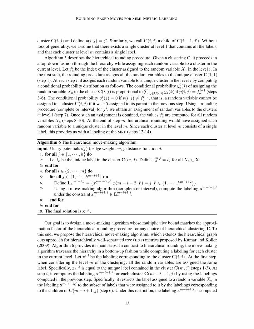
Algorithm 6 The hierarchical move-making algorithm.input Unary potentials θa(·), edge weights wab, distance function d.
1: for all j ∈ {1, · · · , h} do2: Let lk be the unique label in the cluster C(m, j). Define xm,j
a = lk for all Xa ∈ X.3: end for4: for all i ∈ {2, · · · ,m} do5: for all j ∈ {1, · · · , hm−i+1} do6: Define Lm−i+1,j
a = {xm−i+2,j′a , p(m− i+ 2, j′) = j, j′ ∈ {1, · · · , hm−i+2}}.
7: Using a move-making algorithm (complete or interval), compute the labeling xm−i+1,j
under the constraint xm−i+1,ja ∈ Lm−i+1,j
a .8: end for9: end for
10: The final solution is x1,1.
Our goal is to design a move-making algorithm whose multiplicative bound matches the approxi-mation factor of the hierarchical rounding procedure for any choice of hierarchical clustering C. Tothis end, we propose the hierarchical move-making algorithm, which extends the hierarchical graphcuts approach for hierarchically well-separated tree (HST) metrics proposed by Kumar and Koller(2009). Algorithm 6 provides its main steps. In contrast to hierarchical rounding, the move-makingalgorithm traverses the hierarchy in a bottom-up fashion while computing a labeling for each clusterin the current level. Let xi,j be the labeling corresponding to the cluster C(i, j). At the first step,when considering the level m of the clustering, all the random variables are assigned the samelabel. Specifically, xm,j
a is equal to the unique label contained in the cluster C(m, j) (steps 1-3). Atstep i, it computes the labeling xm−i+1,j for each cluster C(m − i + 1, j) by using the labelingscomputed in the previous step. Specifically, it restricts the label assigned to a random variable Xa inthe labeling xm−i+1,j to the subset of labels that were assigned to it by the labelings correspondingto the children of C(m− i+1, j) (step 6). Under this restriction, the labeling xm−i+1,j is computed
13
KUMAR AND DOKANIA
by approximately minimizing the energy using a move-making algorithm (step 7). Implicit in ourdescription is the assumption that that we will use a move-making algorithm (complete or interval) instep 7 of Algorithm 6 whose multiplicative bound matches the approximation factor of the roundingprocedure (complete or interval) used in step 7 of Algorithm 5. Note that, unlike the hierarchicalgraph cuts approach (Kumar and Koller, 2009), the hierarchical move-making algorithm can be usedfor any arbitrary clustering and not just the one specified by an HST metric.
The following theorem establishes the theoretical guarantees of the hierarchical move-makingalgorithm and the hierarchical rounding procedure.
Theorem 8 The tight multiplicative bound of the hierarchical move-making algorithm is equal tothe tight approximation factor of the hierarchical rounding procedure.
The proof of the above theorem is given in Appendix C. The following known result is its corollary.
Corollary 9 The multiplicative bound of the hierarchical move-making algorithm is O(1) for anHST metric distance.
The above corollary follows from the approximation factor of the hierarchical rounding procedureproved by Kleinberg and Tardos (1999), but it was independently proved by Kumar and Koller(2009). It is worth noting that the above result was also used to obtain an approximation factor ofO(log h) for the general metric labeling problem by Kleinberg and Tardos (1999) and a matchingmultiplicative bound of O(log h) by Kumar and Koller (2009).
The time complexity of the hierarchical move-making algorithm depends on two factors: (i)the hierarchy, which defines the subproblems; and (ii) whether we use a complete or an intervalmove-making algorithm to solve the subproblems. In what follows, we analyze its worst case timecomplexity over all possible hierarchies. Clearly, since complete move-making is more expensivethan interval move-making, the worst case complexity of hierarchical move-making will be achievedwhen we use complete move-making to solve each subproblem. We begin by noting that eachproblem is defined using a smaller label set. For simplicitly, let us assume that the clusters of thehierarchy are balanced, and that each subproblem is solved over h′ ≤ h labels. It follows that thetotal number of subproblems that we would be required to solve is O((h/h′)(log(h)/ log(h
′))−1). Next,observe that the complexity of the complete move-making algorithms is cubic in the number of labels.Thus, it follows that in order to maximize the total time complexity of hierarchical move-making, weneed to set h′ = h. In other words, hierarchical move-making algorithm is at most as computationallycomplex as the complete move-making algorithm. Recall that the complete move-making complexityis O(nmh3 log(m)). Hence, hierarchical move-making is significantly faster than solving the LP
relaxation.
8. Experiments
We demonstrate the efficacy of rounding-based moves by comparing them to several state of the artmethods using both synthetic and real data.
8.1 Synthetic Experiments
8.1.1 DATA
We generated two synthetic data sets to conduct our experiments. The first data set consists of randomgrid MRFs of size 100 × 100, where each random variable can take one of 10 labels. The unary
14

ROUNDING-BASED MOVES FOR SEMI-METRIC LABELING
potentials were sampled from a uniform distribution over [0, 10]. The edge weights were sampledfrom a uniform distribution over [0, 3]. We considered four types of pairwise potentials: (i) truncatedlinear metric, where the truncation is sampled from a uniform distribution over [1, 5]; (ii) truncatedquadratic semi-metric, where the truncation is sampled from a uniform distribution over [1, 25]; (iii)random metrics, generated by computing the shortest path on graphs whose vertices correspond tothe labels and whose edge lengths are uniformly distributed over [1, 10]; (iv) random semi-metrics,where the distance between two labels is sampled from a uniform distribution over [1, 10]. For eachtype of pairwise potentials, we generated 500 different MRFs.
The second data set is similar to the first one, except that it is defined on a smaller grid of size20× 20. The smaller grid size allows us to test the mixture-of-tree algorithm (Andrew et al., 2011)that is closely related to the serial rounding procedure of Archer et al. (2004). We generated 5different grids by sampling their edge weights from a uniform distribution over [5, 100]. For eachset of edge weights, we use the cut-based decomposition method of Racke (2008) to approximatethe original grid graph using a mixture of tree-structured graphs. We generated three types of unarypotentials by uniformly sampling from the range [0, 100], [100, 1000] and [1000, 10000] respectively.Similar to the first data set, we considered four types of pairwise potentials. For each pair of unarypotential type and pairwise potential type, we generated 100 different MRFs. This provided us with1200 MRFs for each set of edge weights, and a total of 6000 MRFs to perform our experiments.
8.1.2 METHODS
We report results obtained by the following state of the art methods using the first data set: (i) beliefpropagation (BP) (Pearl, 1998); (ii) sequential tree-reweighted message passing (TRW) (Kolmogorov,2006), which optimizes the dual of the LP relaxation, and provides comparable results to other LP
relaxation based approaches; (iii) expansion algorithm (EXP) (Boykov et al., 1999); and (iv) swapalgorithm (SWAP) (Boykov et al., 1998). We compare the above methods to a hierarchy move-makingalgorithm (HIER), where a set of hierarchies is obtained by approximating a given semi-metric as amixture of r-HST metrics using the method proposed by Fakcharoenphol et al. (2003). We refer thereader to (Fakcharoenphol et al., 2003; Kumar and Koller, 2009) for details. Each subproblem of thehierarchical move-making algorithm is solved by interval move-making with interval length q = 1(which corresponds to the expansion algorithm). In addition, for the truncated linear and truncatedquadratic cases, we present results of interval move-making (INT) using the optimal interval lengthreported by Kumar and Torr (2008).
For the second data set, we report the results for all the above methods, as well as the mixture-of-tree (MOT) algorithm. The smaller size of the grid in the second data set allows us to obtain amixture of tree-structured MRFs using the method of Racke (2008), which was not possible for thelarger 100× 100 grid used in the first data set.
8.1.3 RESULTS
Figure 1 shows the results for the first data set. In terms of the energy, TRW is the most accurate.However, it is slow as it optimizes the dual of the LP relaxation. The labelings obtained by BP
have high energy values. The standard move-making algorithms, EXP and SWAP, are fast due tothe use of efficient minimum st-cut solvers. However, they are not as accurate as TRW. For thetruncated linear and quadratic pairwise potentials, INT provides labelings with comparable energy tothose of TRW, and is also computationally efficient. However, for general metrics and semi-metrics,
15
KUMAR AND DOKANIA
0 2 4 6 8 10 124.8
5
5.2
5.4
5.6
5.8
6
6.2
6.4x 10
4
Time (sec)
Energ
y
BPTRWDUALEXPSWAPINTHIER
0 5 10 154
5
6
7
8
9x 10
4
Time (sec)
Energ
y
BPTRWDUALEXPSWAPINTHIER
Truncated Linear Truncated Quadratic
0 2 4 6 8 105.1
5.15
5.2
5.25
5.3
5.35
5.4
5.45x 10
4
Time (sec)
En
erg
y
BPTRWDUALEXPSWAPHIER
0 2 4 6 8 105.1
5.15
5.2
5.25
5.3
5.35
5.4
5.45
5.5x 10
4
Time (sec)
En
erg
y
BPTRWDUALEXPSWAPHIER
Metric Semi-Metric
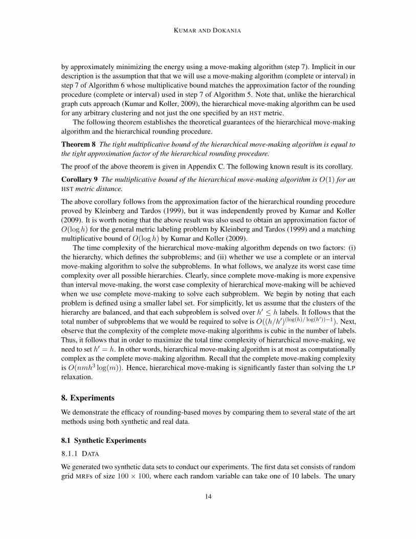
Figure 1: Results for the first synthetic data set. The x-axis shows the time in seconds, while they-axis shows the energy value. The dashed line shows the value of the dual of the LP
obtained by TRW. Best viewed in color.
it is not obvious how to obtain the optimal interval length. The HIER method is more generallyapplicable as there exist standard methods to approximate a semi-metric with a mixture of r-HST
metrics (Fakcharoenphol et al., 2003). It provides very accurate labelings (comparable to TRW),and is efficient in practice as it relies on solving each subproblem using an iterative move-makingalgorithm.
Figure 2 shows the results for the second data set. The results of all the methods are similar tothe first data set. However, the additional MOT algorithm performs very poorly compared to all othermethods. This may be explained by the fact that, while MOT provides the same worst-case guaranteesas serial rounding over all possible metric distance functions, it does not match the accuracy of serialrounding for a given distance function.
16

ROUNDING-BASED MOVES FOR SEMI-METRIC LABELING
Truncated Linear Truncated Quadratic
Metric Semi-Metric
Figure 2: Results for the second synthetic data set. The x-axis shows the time in seconds, whilethe y-axis shows the energy value. The dashed line shows the value of the dual of the LP
obtained by TRW. Best viewed in color.
17

KUMAR AND DOKANIA
8.2 Dense Stereo Correspondence
8.2.1 DATA
Given two epipolar rectified images of the same scene, the problem of dense stereo correspondencerequires us to obtain a correspondence between the pixels of the images. This problem can bemodeled as semi-metric labeling, where the random variables represent the pixels of one of theimages, and the labels represent the disparity values. A disparity label li for a random variableXa representing a pixel (ua, va) of an image indicates that its corresponding pixel lies in location(ua + i, va). For the above problem, we use the unary potentials and edge weights that are specifiedby Szeliski et al. (2008). We use two types of pairwise potentials: (i) truncated linear with thetruncation set at 4; and (ii) truncated quadratic with the truncation set at 16.
8.2.2 METHODS
We report results on all the baseline methods that were used in the synthetic experiments, namely, BP,TRW, EXP, and SWAP. Since the pairwise potentials are either truncated linear or truncated quadratic,we report results for the interval move-making algorithm INT, which uses the optimal value of theinterval length. We also show the results obtained by the hierarchical move-making algorithm (HIER),where once again the hierarchies are obtained by approximating the semi-metric as a mixture ofr-HST metrics.
8.2.3 RESULTS
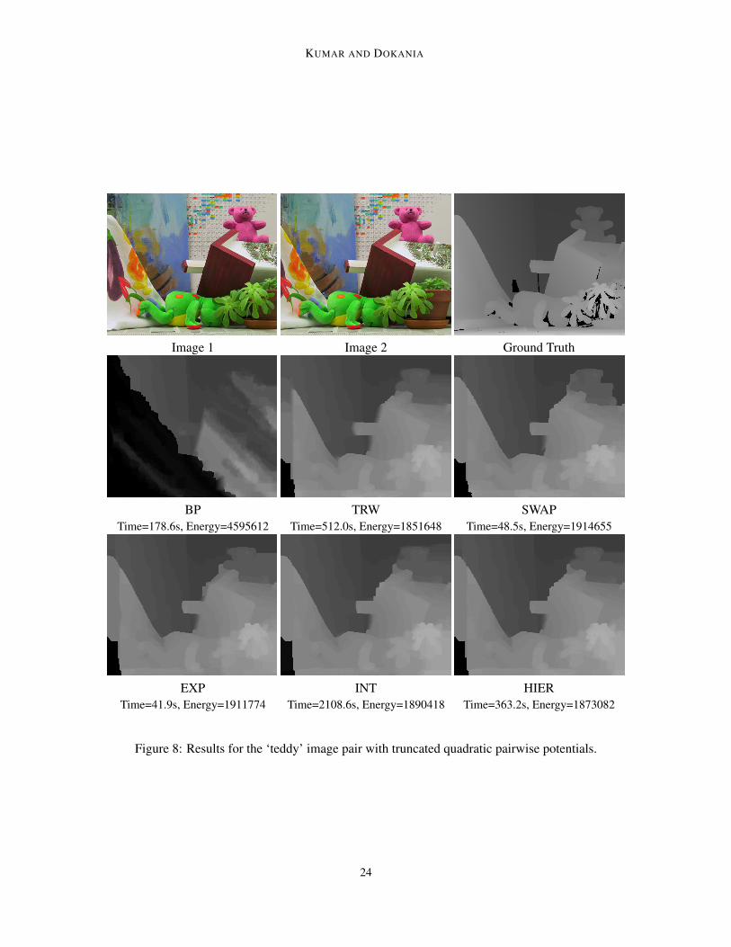
Figure 3-Figure 8 shows the results for various standard pairs of images. Note that, similar tothe synthetic experiments, TRW is the most accurate in terms of energy, but it is computationallyinefficient. The results obtained by BP are not accurate. The standard move-making algorithms, EXP
and SWAP, are fast but not as accurate as TRW. Among the rounding-based move-making algorithmsINT is slower as it solves a minimum st-cut problem on a large graph at each iteration. In contrast,HIER uses an interval length of 1 for each subproblem and is therefore more efficient. The energyobtained by HIER is comparable to TRW.
9. Discussion
For any general distance function that can be used to specify the semi-metric labeling problem, weproved that the approximation factor of a large family of parallel rounding procedures is matched bythe multiplicative bound of move-making algorithms. This generalizes previously known results onthe guarantees of move-making algorithms in two ways: (i) in contrast to previous results (Kumarand Koller, 2009; Kumar and Torr, 2008; Veksler, 1999) that focused on special cases of distancefunctions, our results are applicable to arbitrary semi-metric distance functions; and (ii) the guaranteesprovided by our theorems are tight. Our experiments confirm that the rounding-based move-makingalgorithms provide similar accuracy to the LP relaxation, while being significantly faster due to theuse of efficient minimum st-cut solvers.
Several natural questions arise. What is the exact characterization of the rounding procedures forwhich it is possible to design matching move-making algorithms? Can we design rounding-basedmove-making algorithms for other combinatorial optimization problems? Answering these questions
18

ROUNDING-BASED MOVES FOR SEMI-METRIC LABELING
Image 1 Image 2 Ground Truth
BP TRW SWAPTime=9.1s, Energy=686350 Time=55.8s, Energy=654128 Time=4.4s, Energy=668031
EXP INT HIERTime=3.3s, Energy=657005 Time=87.2s, Energy=656945 Time=34.6s, Energy=654557
Figure 3: Results for the ‘tsukuba’ image pair with truncated linear pairwise potentials.
19
KUMAR AND DOKANIA
Image 1 Image 2 Ground Truth
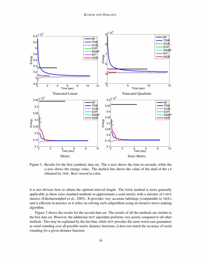
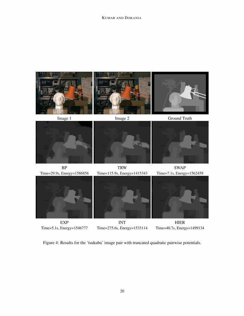
BP TRW SWAPTime=29.9s, Energy=1586856 Time=115.9s, Energy=1415343 Time=7.1s, Energy=1562459
EXP INT HIERTime=5.1s, Energy=1546777 Time=275.6s, Energy=1533114 Time=40.7s, Energy=1499134
Figure 4: Results for the ‘tsukuba’ image pair with truncated quadratic pairwise potentials.
20

ROUNDING-BASED MOVES FOR SEMI-METRIC LABELING
Image 1 Image 2 Ground Truth
BP TRW SWAPTime=16.4s, Energy=3003629 Time=105.2s, Energy=2943481 Time=7.7s, Energy=2954819
EXP INT HIERTime=11.5s, Energy=2953157 Time=273.1s, Energy=2959133 Time=105.7s, Energy=2946177
Figure 5: Results for the ‘venus’ image pair with truncated linear pairwise potentials.
21

KUMAR AND DOKANIA
Image 1 Image 2 Ground Truth
BP TRW SWAPTime=54.3s, Energy=4183829 Time=223.0s, Energy=3080619 Time=22.8s, Energy=3240891
EXP INT HIERTime=30.3s, Energy=3326685 Time=522.3s, Energy=3216829 Time=113s, Energy=3210882
Figure 6: Results for the ‘venus’ image pair with truncated quadratic pairwise potentials.
22

ROUNDING-BASED MOVES FOR SEMI-METRIC LABELING
Image 1 Image 2 Ground Truth
BP TRW SWAPTime=47.5s, Energy=1771965 Time=317.7s, Energy=1605057 Time=35.2s, Energy=1606891
EXP INT HIERTime=26.5s, Energy=1603057 Time=878.5s, Energy=1606558 Time=313.7s, Energy=1596279
Figure 7: Results for the ‘teddy’ image pair with truncated linear pairwise potentials.
23
KUMAR AND DOKANIA
Image 1 Image 2 Ground Truth
BP TRW SWAPTime=178.6s, Energy=4595612 Time=512.0s, Energy=1851648 Time=48.5s, Energy=1914655
EXP INT HIERTime=41.9s, Energy=1911774 Time=2108.6s, Energy=1890418 Time=363.2s, Energy=1873082
Figure 8: Results for the ‘teddy’ image pair with truncated quadratic pairwise potentials.
24

ROUNDING-BASED MOVES FOR SEMI-METRIC LABELING
will not only expand our theoretical understanding, but also result in the development of efficient andaccurate algorithms.
Acknowledgments
This work is partially funded by the European Research Council under the European Community’sSeventh Framework Programme (FP7/2007-2013)/ERC Grant agreement number 259112.
Appendix A. Proof of Theorem 1
We first establish the theoretical property of the complete move-making algorithm using the followinglemma.
Lemma 10 The tight multiplicative bound of the complete move-making algorithm is equal to thesubmodular distortion of the distance function.
Proof The submodular distortion of a distance function d is obtained by computing its tightestsubmodular overestimation as follows:
d = argmind′
t (7)
s.t. d′(li, lj) ≤ td(li, lj), ∀li, lj ∈ L,
d′(li, lj) ≥ d(li, lj),∀li, lj ∈ L,
d′(li, lj) + d′(li+1, lj+1) ≤ d′(li, lj+1) + d′(li+1, lj), ∀li, lj ∈ L\{lh}.
In order to prove the theorem, it is important to note that the definition of submodular distancefunction implies the following:
d(li, lj) + d(li′ , lj′) ≤ d(li, lj′) + d(li′ , lj),∀i′ > i, j′ > j.
A simple proof for the above claim can be found in (Flach and Schlesinger, 2006).We denote the submodular distortion of d by B. By definition, it follows that
d(li, lj) ≤ d(li, lj) ≤ Bd(li, lj),∀li, lj ∈ L. (8)
We denote an optimal labeling of the original semi-metric labeling problem as x∗, that is,
x∗ = argminx∈Ln
∑Xa∈X
θa(xa) +∑
(Xa,Xb)∈E
wabd(xa, xb). (9)
As the semi-metric labeling problem is NP-hard, an optimal labeling x∗ cannot be computed efficientlyusing any known algorithm. In order to obtain an approximate solution x, the complete move-makingalgorithm replaces the original distance function d by its submodular overestimation d, that is,
x = argminx∈Ln
∑Xa∈X
θa(xa) +∑
(Xa,Xb)∈E
wabd(xa, xb). (10)
25
KUMAR AND DOKANIA
Since the pairwise potentials in the above problem are submodular, the approximate solution x canbe obtained by solving a single minimum st-cut problem using the method of Flach and Schlesinger(2006). Using inequality (8), it follows that∑
Xa∈Xθa(xa) +
∑(Xa,Xb)∈E
wabd(xa, xb)
≤∑
Xa∈Xθa(xa) +
∑(Xa,Xb)∈E
wabd(xa, xb)
≤∑
Xa∈Xθa(x
∗a) +
∑(Xa,Xb)∈E
wabd(x∗a, x∗b)
≤∑
Xa∈Xθa(x
∗a) +B
∑(Xa,Xb)∈E
wabd(x∗a, x∗b).
The above inequality proves that the multiplicative bound of the complete move-making algorithm isat most B. In order to prove that it is exactly equal to B, we need to construct an example for whichthe bound is tight. To this end, let lk and lk′ be two labels in the set L such that k < k′ and
d(lk, lk′)
d(lk, lk′)= B.
Since B is the minimum possible value of the maximum ratio of the estimated distance d to theoriginal distance d, such a pair of labels must exist (otherwise, the submodular distortion can bereduced further). Let us assume that there exists an lj ∈ L such that j < k. Other cases (wherej > k′ or k < j < k′) can be handled similarly. Note that since d is submodular, it follows that
d(lk, lj) + d(lj , lk′) ≥ d(lk, lk′). (11)
We define a semi-metric labeling problem over two random variables Xa and Xb connected by anedge with weight wab = 1. The unary potentials are defined as follows:
θa(i) =
0, if i = k,
d(lk,lk′ )+d(lk,lj)−d(lj ,lk′ )2 , if i = j,∞ otherwise,
θb(i) =
0, if i = k′,
d(lk,lk′ )−d(lk,lj)+d(lj ,lk′ )2 , if i = j,∞ otherwise.
For the above semi-metric labeling problem, it can be verified that an optimal solution x∗ ofproblem (9) is the following: x∗a = lk and x∗b = lk′ . Furthermore, using inequality (11), it can beshown that the following is an optimal solution of problem (10): xa = lj and xb = lj . In other words,x is a valid approximate labeling provided by the complete move-making algorithm. The labelingsx∗ and x satisfy the following equality:∑
Xa∈Xθa(xa) +
∑(Xa,Xb)∈E
wabd(xa, xb) =∑
Xa∈Xθa(x
∗a) +B
∑(Xa,Xb)∈E
wabd(x∗a, x∗b).
26
ROUNDING-BASED MOVES FOR SEMI-METRIC LABELING
Therefore, the tight multiplicative bound of the complete move-making algorithm is exactly equal tothe submodular distortion of the distance function d.
We now turn our attention to the complete rounding procedure for the LP relaxation. Before wecan establish its tight approximation factor, we need to compute the expected distance between thelabels assigned to a pair of neighboring random variables. Recall that, in our notation, we denote afeasible solution of the LP relaxation by y. For any feasible solution y, we define ya as the vectorwhose elements are the unary variables of y for the random variable Xa ∈ X, that is,
ya = [ya(i), ∀li ∈ L]. (12)
Similarly, we define yab as the vector whose elements are the pairwise variables of y for theneighboring random variables (Xa, Xb) ∈ E, that is,
yab = [yab(i, j),∀li, lj ∈ L]. (13)
Furthermore, using ya, we define Ya as
Ya(i) =
i∑j=1
ya(j).
In other words, if ya is interpreted as the probability distribution over the labels of Xa, then Ya isthe corresponding cumulative distribution.
Given a feasible solution y, we denote the integer solution obtained using the complete roundingprocedure as y. The distance between the two labels encoded by vectors ya and yb will be denotedby d(ya, yb). In other words, if fa and fb are the indices of the labels assigned to Xa and Xb (that is,ya(fa) = 1 and yb(fb) = 1), then d(ya, yb) = d(lfa , lfb).
The following shorthand notation would be useful for our analysis.
D1(i) =1
2(d(li, l1) + d(li, lh)− d(li+1, l1)− d(li+1, lh)) ,∀i ∈ {1, · · · , h− 1}, (14)
D2(i, j) =1
2(d(li, lj+1) + d(li+1, lj)− d(li, lj)− d(li+1, lj+1)) , ∀i, j ∈ {1, · · · , h− 1}.
Using the above notation, we can state the following lemma on the expected distance of therounded solution for two neighboring random variables.
Lemma 11 Let y be a feasible solution of the LP relaxation, Ya and Yb be cumulative distributionsof ya and yb, and y be the integer solution obtained by the complete rounding procedure for y. Then,the following equation holds true:
E(d(ya, yb)) =
h−1∑i=1
Ya(i)D1(i) +
h−1∑j=1
Yb(j)D1(j) +
h−1∑i=1
h−1∑j=1
|Ya(i)− Yb(j)|D2(i, j).
27
KUMAR AND DOKANIA
Proof We define fa and fb to be the indices of the labels assigned to Xa and Xb by the roundedinteger solution y. In other words, ya(i) = 1 if and only if i = fa and yb(j) = 1 if and only ifj = fb. We define binary variables za(i) and zb(j) as follows:
za(i) =
{1 if i ≤ fa,0 otherwise,
zb(j) =
{1 if j ≤ fb,0 otherwise.
For complete rounding, it can be verified that
E(za(i)) = Ya(i). (15)
Furthermore, we also define binary variables zab(i, j) that indicate whether i and j are containedwithin the interval defined by fa and fb. Formally,
zab(i, j) =
{1 if min{i, j} ≥ min{fa, fb} and max{i, j} < max{fa, fb},0 otherwise.
For complete rounding, it can be verified that
E(zab(i, j)) = |Ya(i)− Yb(j)|. (16)
Using the result of Flach and Schlesinger (2006), we know that
d(ya, yb) =
h−1∑i=1
za(i)D1(i) +
h−1∑j=1
zb(j)D1(j) +
h−1∑i=1
h−1∑j=1
zab(i, j)D2(i, j).
The proof of the lemma follows by taking the expectation of the LHS and the RHS of the aboveequation and simplifying the RHS using the linearity of expectation and equations (15) and (16).
In order to state the next lemma, we require the definition of uncrossing pairwise variables. Givenunary variables ya and yb, the pairwise variable vector y′ab is called uncrossing with respect to ya
and yb if it satisfies the following properties:h∑
j=1
y′ab(i, j) = ya(i), ∀i ∈ {1, 2, · · · , h},
h∑i=1
y′ab(i, j) = yb(i),∀j ∈ {1, 2, · · · , h},
y′ab(i, j) ≥ 0, ∀i, j ∈ {1, 2, · · · , h},min{y′ab(i, j′), y′ab(i′, j)} = 0,∀i, j, i′, j′ ∈ {1, 2, · · · , h}, i < i′, j < j′. (17)
The following lemma establishes a connection between the expected distance between the labelsassigned by complete rounding and the pairwise cost specified by uncrossing pairwise variables.
Lemma 12 Let y be a feasible solution of the LP relaxation, and y be the integer solution obtainedby the complete rounding procedure for y. Furthermore, let y′ab be uncrossing pairwise variableswith respect to ya and yb. Then, the following equation holds true:
E(d(ya, yb)) =h∑
i=1
h∑j=1
d(li, lj)y′ab(i, j).
28

ROUNDING-BASED MOVES FOR SEMI-METRIC LABELING
Proof We define Ya and Yb to be the cumulative distributions corresponding to ya and yb respec-tively. We claim that the uncrossing property (17) implies the following condition:
i′∑i=1
j′∑j=1
y′ab(i, j) = min{Ya(i′), Yb(j′)},∀i′, j′ ∈ {1, · · · , h}. (18)
To prove this claim, assume that Ya(i′) < Yb(j′). The other cases can be handled similarly. Since
y′ab satisfies the constraints of the LP relaxation, it follows that:
h∑i=1
j′∑j=1
y′ab(i, j) = Yb(j′),
i′∑i=1
h∑j=1
y′ab(i, j) = Ya(i′). (19)
Since the LHS of equality (18) is less than or equal to the LHS of both the above equations, it followsthat
i′∑i=1
j′∑j=1
y′ab(i, j) ≤ min{Ya(i′), Yb(j′)}. (20)
Therefore, there must exist a k > i′ and k′ ≤ j′ such that y′ab(k, k′) 6= 0. Otherwise, the LHS
in the above inequality will be exactly equal to Yb(j′), which would result in a contradiction. Bythe uncrossing property (17), we know that min{y′ab(i, j), y′ab(k, k′)} = 0 if i ≤ i′ and j > j′.Therefore, y′ab(i, j) = 0 for all i ≤ i′ and j > j′, which proves the claim.
Combining equations (19) and (20), we get the following:
i′∑i=1
h∑j=j′+1
y′ab(i, j) +
h∑i=i′+1
j′∑j=1
y′ab(i, j) = |Ya(i)− Yb(j)|,∀i′, j′ ∈ {1, · · · , h}.
By solving for y′ab using the above equations, we get
h∑i=1
h∑j=1
d(li, lj)y′ab(i, j) =
h−1∑i=1
Ya(i)D1(i) +h−1∑j=1
Yb(j)D1(j) +h−1∑i=1
h−1∑j=1
|Ya(i)− Yb(j)|D2(i, j).
Using the previous lemma, this proves that
E(d(ya, yb)) =
h∑i=1
h∑j=1
d(li, lj)y′ab(i, j).
Our next lemma establishes that uncrossing pairwise variables are optimal for submodulardistance functions.
29

KUMAR AND DOKANIA
Lemma 13 Let y′ab be the uncrossing pairwise variables with respect to the unary variables ya andyb. Let d : L × L → R+ be a submodular distance function. Then the following condition holdstrue:
y′ab = argminyab
h∑i=1
h∑j=1
d(i, j)yab(i, j), (21)
s.t.h∑
j=1
yab(i, j) = ya(i), ∀i ∈ {1, · · · , h},
h∑i=1
yab(i, j) = yb(j), ∀j ∈ {1, · · · , h},
yab(i, j) ≥ 0, ∀i, j ∈ {1, · · · , h}.
Proof We prove the lemma by contradiction. Suppose that the optimal solution to the above problemis y′′ab, which is not uncrossing. Let
min{y′′ab(i, j′), y′′ab(i′, j)} = λ 6= 0,
where i < i′ and j < j′. Since d is submodular, it implies that
d(li, lj) + d(li′ , lj′) ≤ d(li, lj′) + d(li′ , lj).
Therefore the objective function of problem (21) can be reduced further by the following modification:
y′′ab(i, j′)← y′′ab(i, j
′)− λ, y′′ab(i′, j)← y′′ab(i′, j)− λ,
y′′ab(i, j)← y′′ab(i, j) + λ, y′′ab(i′, j′)← y′′ab(i
′, j′) + λ.
The resulting contradiction proves our claim that the uncrossing pairwise variables y′ab are an optimalsolution of problem (21).
Using the above lemmas, we will now obtain the tight approximation factor of the completerounding procedure.
Lemma 14 The tight approximation factor of the complete rounding procedure is equal to thesubmodular distortion of the distance function.
Proof We denote a feasible fractional solution of the LP relaxation by y and the rounded solution byy. Consider a pair of neighboring random variables (Xa, Xb) ∈ X. We define uncrossing pairwisevariables y′ab with respect to ya and yb. Using Lemmas 12 and 13, the approximation factor of the
30

ROUNDING-BASED MOVES FOR SEMI-METRIC LABELING
complete rounding procedure can be shown to be at most B as follows:
E(d(ya, yb)) =
h∑i=1
h∑j=1
d(li, lj)y′ab(i, j)
≤h∑
i=1
h∑j=1
d(li, lj)y′ab(i, j)
≤h∑
i=1
h∑j=1
d(li, lj)yab(i, j)
≤ B
h∑i=1
h∑j=1
d(li, lj)yab(i, j).
In order to prove that the approximation factor of the complete rounding is exactly B, we need anexample where the above inequality holds as an equality. The key to obtaining a tight example lies inthe Lagrangian dual of problem (7). In order to specify its dual, we need three types of dual variables.The first type, denoted by α(i, j), corresponds to the constraint
d′(li, lj) ≤ td(li, lj).
The second type, denoted by β(i, j), corresponds to the constraint
d′(li, lj) ≥ d(li, lj).
The third type, denoted by γ(i, j), corresponds to the constraint
d′(li, lj) + d′(li+1, lj+1) ≤ d′(li, lj+1) + d′(li+1, lj).
Using the above variables, the dual of problem (7) is given by
max
h∑i=1
h∑j=1
d(li, lj)β(i, j) (22)
s.t.h∑
i=1
h∑j=1
d(li, lj)α(i, j) = 1,
β(i, j) = α(i, j)− γ(i, j − 1)− γ(i− 1, j) + γ(i− 1, j − 1) + γ(i, j),
∀i, j ∈ {1, · · · , h},α(i, j) ≥ 0, β(i, j) ≥ 0, γ(i, j) ≥ 0, ∀i, j ∈ {1, · · · , h}.
We claim that the above dual problem has an optimal solution (α∗,β∗,γ∗) that satisfies the followingproperty:
min{β∗(i, j′), β∗(i′, j)} = 0,∀i, i′, j, j′ ∈ {1, · · · , h}, i < i′, j < j′. (23)
We refer to the optimal dual solution β∗ that satisfies the above property as uncrossing dual variablesas it is analogous to uncrossing pairwise variables. The above claim, namely, the existence of anuncrossing optimal dual solution, can be proved by contradiction as follows. Suppose there exists no
31
KUMAR AND DOKANIA
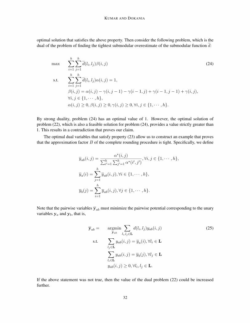
optimal solution that satisfies the above property. Then consider the following problem, which is thedual of the problem of finding the tightest submodular overestimate of the submodular function d:
maxh∑
i=1
h∑j=1
d(li, lj)β(i, j) (24)
s.t.h∑
i=1
h∑j=1
d(li, lj)α(i, j) = 1,
β(i, j) = α(i, j)− γ(i, j − 1)− γ(i− 1, j) + γ(i− 1, j − 1) + γ(i, j),
∀i, j ∈ {1, · · · , h},α(i, j) ≥ 0, β(i, j) ≥ 0, γ(i, j) ≥ 0, ∀i, j ∈ {1, · · · , h}.
By strong duality, problem (24) has an optimal value of 1. However, the optimal solution ofproblem (22), which is also a feasible solution for problem (24), provides a value strictly greater than1. This results in a contradiction that proves our claim.
The optimal dual variables that satisfy property (23) allow us to construct an example that provesthat the approximation factor B of the complete rounding procedure is tight. Specifically, we define
yab(i, j) =α∗(i, j)∑h
i′=1
∑hj′=1 α
∗(i′, j′),∀i, j ∈ {1, · · · , h},
ya(i) =h∑
j=1
yab(i, j), ∀i ∈ {1, · · · , h},
yb(j) =h∑
i=1
yab(i, j), ∀j ∈ {1, · · · , h}.
Note that the pairwise variables yab must minimize the pairwise potential corresponding to the unaryvariables ya and yb, that is,
yab = argminyab
∑li,lj∈L
d(li, lj)yab(i, j) (25)
s.t.∑lj∈L
yab(i, j) = ya(i),∀li ∈ L
∑li∈L
yab(i, j) = yb(j),∀lj ∈ L
yab(i, j) ≥ 0, ∀li, lj ∈ L.
If the above statement was not true, then the value of the dual problem (22) could be increasedfurther.
32

ROUNDING-BASED MOVES FOR SEMI-METRIC LABELING
We also define the following pairwise variables:
y′ab(i, j) =β∗(i, j)∑h
i′=1
∑hj′=1 β
∗(i′, j′), ∀i, j ∈ {1, · · · , h},
y′a(i) =h∑
j=1
y′ab(i, j),∀i ∈ {1, · · · , h},
y′b(j) =h∑
i=1
y′ab(i, j),∀j ∈ {1, · · · , h}.
It can be verified that
y′a(i) = ya(i), y′b(j) = yb(j),∀i, j ∈ {1, · · · , h}.
The above condition follows from the constraints of problem (22). Due to the uncrossing property ofβ∗, the pairwise variables y′ab are uncrossing with respect to ya and yb. By Lemma 12, this impliesthat
E(d(ya, yb)) =h∑
i=1
h∑j=1
d(li, lj)y′ab(i, j),
where ya and yb are integer solutions obtained by the complete rounding procedure. By strongduality, it follows that
E(d(ya, yb)) = B
h∑i=1
h∑j=1
d(li, lj)yab(i, j). (26)
The existence of an example that satisfies properties (25) and (26) implies that the tight approximationfactor of the complete rounding procedure is B.
Lemmas 10 and 14 together prove Theorem 1.
Appendix B. Proof of Theorem 3
We begin by establishing the theoretical properties of the interval-move making algorithm. Recallthat, given an interval of labels I = {ls, · · · , le} of at most q consecutive labels and a labeling x, wedefine Ia = I ∪ {xa} for all random variables Xa ∈ X. In order to use the interval move-makingalgorithm, we compute a submodular distance function dxa,xb
: Ia × Ib → R+ for all pairs ofneighboring random variables (Xa, Xb) ∈ E as follows:
dxa,xb= argmin
d′t (27)
s.t. d′(li, lj) ≤ td(li, lj), ∀li ∈ Ia, lj ∈ Ib,
d′(li, lj) ≥ d(li, lj),∀li ∈ Ia, lj ∈ Ib,
d′(li, lj) + d′(li+1, lj+1) ≤ d′(li, lj+1) + d′(li+1, lj), ∀li, lj ∈ I\{le},d′(li, le) + d′(li+1, xb) ≤ d′(li, xb) + d′(li+1, le), ∀li ∈ I\{le},d′(le, lj) + d′(xa, lj+1) ≤ d′(le, lj+1) + d′(xa, lj), ∀lj ∈ I\{le},d′(le, le) + d(xa, xb) ≤ d′(le, xb) + d′(xa, le).
33

KUMAR AND DOKANIA
For any interval I and labeling x, we define the following sets:
V(x, I) = {Xa|Xa ∈ X, xa ∈ I},A(x, I) = {(Xa, Xb)|(Xa, Xb) ∈ E, xa ∈ I, xb ∈ I},B1(x, I) = {(Xa, Xb)|(Xa, Xb) ∈ E, xa ∈ I, xb /∈ I},B2(x, I) = {(Xa, Xb)|(Xa, Xb) ∈ E, xa /∈ I, xb ∈ I},B(x, I) = B1(x) ∪B2(x).
In other words, V(x, I) is the set of all random variables whose label belongs to the interval I.Similarly, A(x, I) is the set of all neighboring random variables such that the labels assigned to boththe random variables belong to the interval I. The set B(x, I) contains the set of all neighboringrandom variables such that only one of the two labels assigned to the two random variables belongsto the interval I. Given the set of all intervals I and a labeling x, we define the following for allxa, xb ∈ L:
D(xa, xb; xa, xb) =∑
I∈I,A(x,I)3(Xa,Xb)
dxa,xb(xa, xb)
+∑
I∈I,B1(x,I)3(Xa,Xb)
dxa,xb(xa, xb)
+∑
I∈I,B2(x,I)3(Xa,Xb)
dxa,xb(xa, xb).
Using the above notation, we are ready to state the following lemma on the theoretical guaranteeof the interval move-making algorithm.
Lemma 15 The tight multiplicative bound of the interval move-making algorithm is equal to
1
qmax
xa,xb,xa,xb∈L,xa 6=xb
D(xa, xb; xa, xb)
d(xa, xb).
Proof We denote an optimal labeling by x∗ and the estimated labeling by x. Let t ∈ [1, q] bea uniformly distributed random integer. Using t, we define the following set of non-overlappingintervals:
It = {[1, t], [t+ 1, t+ q], · · · , [., h]}.
For each interval I ∈ It, we define a labeling xI as follows:
xIa =
{x∗a if x∗a ∈ I,xa otherwise.
Since x is the labeling obtained after the interval move-making algorithm converges, it follows that∑Xa∈X
θa(xa) +∑
(Xa,Xb)∈E
wabdxa,xb(xa, xb) ≤
∑Xa∈X
θa(xIa) +
∑(Xa,Xb)∈E
wabdxa,xb(xIa, x
Ib).
34
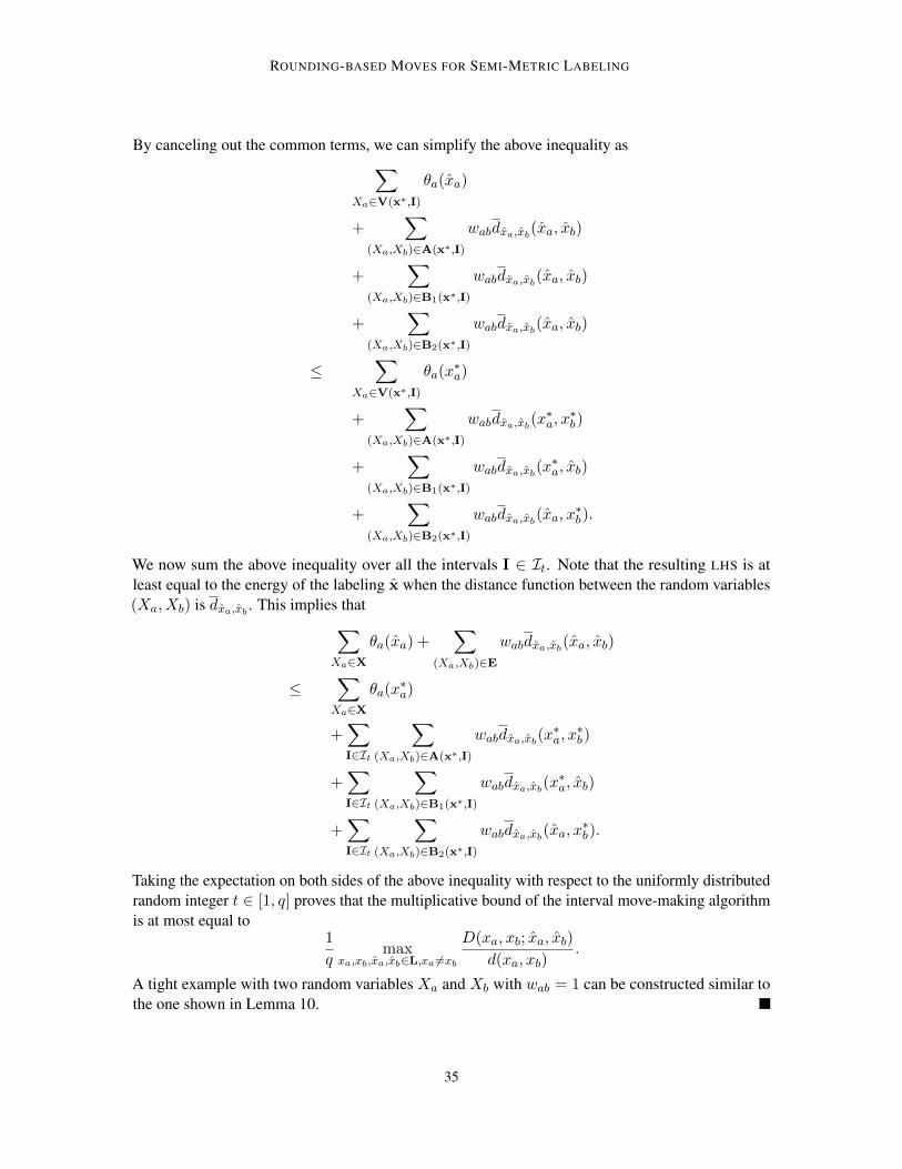
ROUNDING-BASED MOVES FOR SEMI-METRIC LABELING
By canceling out the common terms, we can simplify the above inequality as∑Xa∈V(x∗,I)
θa(xa)
+∑
(Xa,Xb)∈A(x∗,I)
wabdxa,xb(xa, xb)
+∑
(Xa,Xb)∈B1(x∗,I)
wabdxa,xb(xa, xb)
+∑
(Xa,Xb)∈B2(x∗,I)
wabdxa,xb(xa, xb)
≤∑
Xa∈V(x∗,I)
θa(x∗a)
+∑
(Xa,Xb)∈A(x∗,I)
wabdxa,xb(x∗a, x
∗b)
+∑
(Xa,Xb)∈B1(x∗,I)
wabdxa,xb(x∗a, xb)
+∑
(Xa,Xb)∈B2(x∗,I)
wabdxa,xb(xa, x
∗b).
We now sum the above inequality over all the intervals I ∈ It. Note that the resulting LHS is atleast equal to the energy of the labeling x when the distance function between the random variables(Xa, Xb) is dxa,xb
. This implies that∑Xa∈X
θa(xa) +∑
(Xa,Xb)∈E
wabdxa,xb(xa, xb)
≤∑
Xa∈Xθa(x
∗a)
+∑I∈It
∑(Xa,Xb)∈A(x∗,I)
wabdxa,xb(x∗a, x
∗b)
+∑I∈It
∑(Xa,Xb)∈B1(x∗,I)
wabdxa,xb(x∗a, xb)
+∑I∈It
∑(Xa,Xb)∈B2(x∗,I)
wabdxa,xb(xa, x
∗b).
Taking the expectation on both sides of the above inequality with respect to the uniformly distributedrandom integer t ∈ [1, q] proves that the multiplicative bound of the interval move-making algorithmis at most equal to
1
qmax
xa,xb,xa,xb∈L,xa 6=xb
D(xa, xb; xa, xb)
d(xa, xb).
A tight example with two random variables Xa and Xb with wab = 1 can be constructed similar tothe one shown in Lemma 10.
35

KUMAR AND DOKANIA
We now turn our attention to the interval rounding procedure. Let y be a feasible solution of theLP relaxation, and y be the integer solution obtained using interval rounding. Once again, we definethe unary variable vector ya and the pairwise variable vector yab as specified in equations (12) and(13) respectively. Similar to the previous appendix, we denote the expected distance between ya andyb as d(ya, yb).
Given an interval I = {ls, · · · , le} of at most q consecutive labels, we define a vector YIa for
each random variable Xa as follows:
Y Ia (i) =
s+i−1∑j=s
ya(j), ∀i ∈ {1, · · · , e− s+ 1}.
In other words, YIa is the cumulative distribution of ya within the interval I. Furthermore, for each
pair of neighboring random variables (Xa, Xb) ∈ E we define
ZIab = max{Y I
a (e− s+ 1), Y Ib (e− s+ 1)} −min{Y I
a (e− s+ 1), Y Ib (e− s+ 1)},
ZIa(i) = min{Y I
a (i), YIb (e− s+ 1)}, ∀i ∈ {1, · · · , e− s+ 1},
ZIb (j) = min{Y I
b (j), YIa (e− s+ 1)}, ∀j ∈ {1, · · · , e− s+ 1}.
The following shorthand notation would be useful to concisely specify the exact form of d(ya, yb).
DI0 = max
li,lj ,|{li,lj}∩I|=1d(li, lj),
DI1(i) =
1
2(d(ls+i−1, ls) + d(ls+i−1, le)− d(ls+i, ls)− d(ls+i, le)) ,∀i ∈ {1, · · · , e− s},
DI2(i, j) =
1
2(d(ls+i−1, ls+j) + d(ls+i, ls+j−1)− d(ls+i−1, ls+j−1)− d(ls+i, ls+j)) ,
∀i, j ∈ {1, · · · , e− s}.
In other words, DI0 is the maximum distance between two labels such that only one of the two labels
lies in the interval I. The terms DI1 and DI
2 are analogous to the terms defined in equation (14).Using the above notation, we can state the following lemma on the expected distance of the roundedsolution for two neighboring random variables.
Lemma 16 Let y be a feasible solution of the LP relaxation, and y be the integer solution obtainedby the interval rounding procedure for y using the set of intervals I. Then, the following inequalityholds true:
E(d(ya, yb)) ≤1
q
∑I={ls,··· ,le}∈I
ZIabD
I0 +
e−s∑i=1
ZIa(i)D
I1(i) +
e−s∑j=1
ZIb (j)D
I1(j)+
e−s∑i=1
e−s∑j=1
|ZIa(i)− ZI
b (j)|DI2(i, j)
.
Proof We begin the proof by establishing the probability of a random variable Xa being assigneda label in an iteration of the interval rounding procedure. The total number of intervals in the set
36
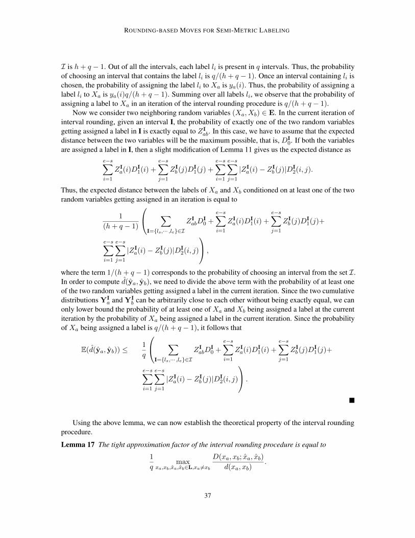
ROUNDING-BASED MOVES FOR SEMI-METRIC LABELING
I is h+ q − 1. Out of all the intervals, each label li is present in q intervals. Thus, the probabilityof choosing an interval that contains the label li is q/(h+ q − 1). Once an interval containing li ischosen, the probability of assigning the label li to Xa is ya(i). Thus, the probability of assigning alabel li to Xa is ya(i)q/(h+ q − 1). Summing over all labels li, we observe that the probability ofassigning a label to Xa in an iteration of the interval rounding procedure is q/(h+ q − 1).
Now we consider two neighboring random variables (Xa, Xb) ∈ E. In the current iteration ofinterval rounding, given an interval I, the probability of exactly one of the two random variablesgetting assigned a label in I is exactly equal to ZI
ab. In this case, we have to assume that the expecteddistance between the two variables will be the maximum possible, that is, DI
0. If both the variablesare assigned a label in I, then a slight modification of Lemma 11 gives us the expected distance as
e−s∑i=1
ZIa(i)D
I1(i) +
e−s∑j=1
ZIb (j)D
I1(j) +
e−s∑i=1
e−s∑j=1
|ZIa(i)− ZI
b (j)|DI2(i, j).
Thus, the expected distance between the labels of Xa and Xb conditioned on at least one of the tworandom variables getting assigned in an iteration is equal to
1
(h+ q − 1)
∑I={ls,··· ,le}∈I
ZIabD
I0 +
e−s∑i=1
ZIa(i)D
I1(i) +
e−s∑j=1
ZIb (j)D
I1(j)+
e−s∑i=1
e−s∑j=1
|ZIa(i)− ZI
b (j)|DI2(i, j)
,
where the term 1/(h+ q − 1) corresponds to the probability of choosing an interval from the set I.In order to compute d(ya, yb), we need to divide the above term with the probability of at least oneof the two random variables getting assigned a label in the current iteration. Since the two cumulativedistributions YI
a and YIb can be arbitrarily close to each other without being exactly equal, we can
only lower bound the probability of at least one of Xa and Xb being assigned a label at the currentiteration by the probability of Xa being assigned a label in the current iteration. Since the probabilityof Xa being assigned a label is q/(h+ q − 1), it follows that
E(d(ya, yb)) ≤1
q
∑I={ls,··· ,le}∈I
ZIabD
I0 +
e−s∑i=1
ZIa(i)D
I1(i) +
e−s∑j=1
ZIb (j)D
I1(j)+
e−s∑i=1
e−s∑j=1
|ZIa(i)− ZI
b (j)|DI2(i, j)
.
Using the above lemma, we can now establish the theoretical property of the interval roundingprocedure.
Lemma 17 The tight approximation factor of the interval rounding procedure is equal to
1
qmax
xa,xb,xa,xb∈L,xa 6=xb
D(xa, xb; xa, xb)
d(xa, xb).
37
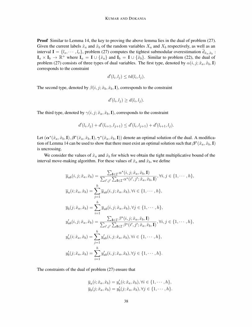
KUMAR AND DOKANIA
Proof Similar to Lemma 14, the key to proving the above lemma lies in the dual of problem (27).Given the current labels xa and xb of the random variables Xa and Xb respectively, as well as aninterval I = {ls, · · · , le}, problem (27) computes the tightest submodular overestimation dxa,xb
:Ia × Ib → R+ where Ia = I ∪ {xa} and Ib = I ∪ {xb}. Similar to problem (22), the dual ofproblem (27) consists of three types of dual variables. The first type, denoted by α(i, j; xa, xb, I)corresponds to the constraint
d′(li, lj) ≤ td(li, lj).
The second type, denoted by β(i, j; xb, xb, I), corresponds to the constraint
d′(li, lj) ≥ d(li, lj).
The third type, denoted by γ(i, j; xa, xb, I), corresponds to the constraint
d′(li, lj) + d′(li+1, lj+1) ≤ d′(li, lj+1) + d′(li+1, lj).
Let (α∗(xa, xb, I),β∗(xa, xb, I),γ∗(xa, xb, I)) denote an optimal solution of the dual. A modifica-tion of Lemma 14 can be used to show that there must exist an optimal solution such that β∗(xa, xb, I)is uncrossing.
We consider the values of xa and xb for which we obtain the tight multiplicative bound of theinterval move-making algorithm. For these values of xa and xb, we define
yab(i, j; xa, xb) =
∑I∈I α
∗(i, j; xa, xb, I)∑i′,j′∑
I∈I α∗(i′, j′; xa, xb, I)
,∀i, j ∈ {1, · · · , h},
ya(i; xa, xb) =
h∑j=1
yab(i, j; xa, xb),∀i ∈ {1, · · · , h},
yb(j; xa, xb) =
h∑i=1
yab(i, j; xa, xb),∀j ∈ {1, · · · , h},
y′ab(i, j; xa, xb) =
∑I∈I β
∗(i, j; xa, xb, I)∑i′,j′∑
I∈I β∗(i′, j′; xa, xb, I)
,∀i, j ∈ {1, · · · , h},
y′a(i; xa, xb) =h∑
j=1
y′ab(i, j; xa, xb), ∀i ∈ {1, · · · , h},
y′b(j; xa, xb) =h∑
i=1
y′ab(i, j; xa, xb), ∀j ∈ {1, · · · , h}.
The constraints of the dual of problem (27) ensure that
ya(i; xa, xb) = y′a(i; xa, xb),∀i ∈ {1, · · · , h},yb(j; xa, xb) = y′b(j; xa, xb),∀j ∈ {1, · · · , h}.
38
ROUNDING-BASED MOVES FOR SEMI-METRIC LABELING
Given the distributions ya(xa, xb) and yb(xa, xb), we claim that the pairwise variables yab(xa, xb)must minimize the pairwise potentials corresponding to these distributions, that is,
yab(xa, xb) = argminyab
∑li,lj∈L
d(li, lj)yab(i, j)
s.t.∑lj∈L
yab(i, j) = ya(i; xa, xb),∀li ∈ L
∑li∈L
yab(i, j) = yb(j; xa, xb),∀lj ∈ L
yab(i, j) ≥ 0, ∀li, lj ∈ L.
If the above claim was not true, then we could further increase the value of at least one of the duals ofproblem (27) corresponding to some interval I. Furthermore, since y′ab(xa, xb) is constructed usingβ∗(xa, xb, I), which is uncrossing, a modification of Lemma 12 can be used to show that
d(ya(xa, xb), yb(xa, xb)) =∑
li,lj∈Ld(li, lj)y
′ab(i, j; xa, xb).
Here ya(xa, xb) and yb(xa, xb) are the rounded solutions obtained by the interval rounding procedureapplied to ya(xa, xb) and yb(xa, xb).
By duality, it follows that∑li,lj∈L d(li, lj)y
′ab(i, j; xa, xb)∑
li,lj∈L d(li, lj)yab(i, j; xa, xb)≤ 1
qmax
xa,xb,xa,xb∈L,xa 6=xb
D(xa, xb; xa, xb)
d(xa, xb).
Strong duality implies that there must exist a set of variables for which the above inequality holds asan equality. This proves the lemma.
Lemmas 15 and 17 together prove Theorem 3.
Appendix C. Proof of Theorem 8
Proof The proof of the above theorem proceeds in a similar fashion to the previous two theorems,namely, by computing the dual of the problems that are used to obtain the tightest submodularoverestimation of the given distance function. In what follows, we provide a brief sketch of the proofand omit the details.
We start with the hierarchical move-making algorithm. Recall that this algorithm computes alabeling xi,j for each cluster C(i, j) ⊆ L, where C(i, j) denotes the j-th cluster at the i-th level.In order to obtain a labeling xi,j it makes use of the labelings computed at the (i + 1)-th level.Specifically, let Li,j
a = {xi+1,j′a , p(i+1, j′) = j, j′ ∈ {1, · · · , hi+1}}. In other words, Li,j
a is the setof labels that were assigned to the random variable Xa by the labelings corresponding to the childrenof the current cluster C(i, j). In order to compute the labeling xi,j , the algorithm has to choose onelabel from the set Li,j
a . This is achieved either using the complete move-making algorithm or theinterval move-making algorithm. The algorithm is initialized by define xm,j
a = k for all Xa ∈ Xwhere k is the unique label in the cluster C(m, j) The algorithm terminates by computing x1,1,which is the final labeling.
39
KUMAR AND DOKANIA
Let the multiplicative bound corresponding to the computation of xi,j be denoted by Bi,j . Fromthe arguments of Theorems 1 and 3, it follows that there must exist dual variables (α∗(i, j),β∗(i, j),γ∗(i, j))that provide an approximation factor that is exactly equal to Bi,j and β∗(i, j) is uncrossing. For eachcluster C(i, j), we define variables δa(k; i, j) for k ∈ Li,j
a as follows:
δa(k; i, j) =
∑k′∈Li,j
bα∗(k, k′; i, j)∑
l∈Li,ja
∑l′∈Li,j
bα∗(l, l′; i, j)
.
Using the above variables we define unary variables ya(k; i, j) for each k ∈ Li,j as follows:
ya(k; 1, 1) = δa(k; 1, 1),
ya(k; i, j) = ya(xi−1,p(i,j)a ; i− 1, p(i, j))δa(k; i, j).
Similarly, we define variables δb(k′; i, j) for each k′ ∈ Li,jb as follows:
δb(k′; i, j) =
∑k∈Li,j
aα∗(k, k′; i, j)∑
l∈Li,ja
∑l′∈Li,j
bα∗(l, l′; i, j)
.
Using the above variables, we define unary variables yb(k′; i, j) for each k′ ∈ Li,jb as follows:
yb(k′; 1, 1) = δb(k
′; 1, 1),
yb(k′; i, j) = ya(x
i−1,p(i,j)a ; i− 1, p(i, j))δb(k
′; i, j).
Since each cluster in the m-th level contains a single unique label, it follows that
ya = [ya(xm,ja ;m, j),∀j = 1, · · · , h],
yb = [yb(xm,jb ;m, j),∀j = 1, · · · , h],
are valid unary variables for the LP relaxation. It can be shown that applying the hierarchical roundingprocedure on the variables ya and yb provides an approximation factor that is exactly equal to themultiplicative bound of the hierarchical move-making algorithm.
References
T. Ajanthan, R. Hartley, M. Salzmann, and H. Li. Iteratively reweighted graph cut for multi-labelMRFs with non-convex priors. CoRR, 2014.
M. Andrew, M. Hajiaghayi, H. Karloff, and A. Moitra. Capacitated metric labeling. In SODA, 2011.
A. Archer, J. Fakcharoenphol, C. Harrelson, R. Krauthgamer, K. Talvar, and E. Tardos. Approximateclassification via earthmover metrics. In SODA, 2004.
Y. Boykov and V. Kolmogorov. An experimental comparison of min-cut/max-flow algorithms forenergy minimization in vision. PAMI, 2004.
Y. Boykov, O. Veksler, and R. Zabih. Markov random fields with efficient approximations. In CVPR,1998.
40

ROUNDING-BASED MOVES FOR SEMI-METRIC LABELING
Y. Boykov, O. Veksler, and R. Zabih. Fast approximate energy minimization via graph cuts. In ICCV,1999.
C. Chekuri, S. Khanna, J. Naor, and L. Zosin. Approximation algorithms for the metric labelingproblem via a new linear programming formulation. In SODA, 2001.
P. Dokania and M. P. Kumar. Parsimonious labeling. In ICCV, 2015.
J. Fakcharoenphol, S. Rao, and K. Talwar. A tight bound on approximating arbitrary metrics by treemetrics. In STOC, 2003.
B. Flach and D. Schlesinger. Transforming an arbitrary minsum problem into a binary one. Technicalreport, TU Dresden, 2006.
A. Globerson and T. Jaakkola. Fixing max-product: Convergent message passing algorithms forMAP LP-relaxations. In NIPS, 2007.
A. Gupta and E. Tardos. A constant factor approximation algorithm for a class of classificationproblems. In STOC, 2000.
T. Hazan and A. Shashua. Convergent message-passing algorithms for inference over general graphswith convex free energy. In UAI, 2008.
J. Kappes, B. Andres, F. Hamprecht, C. Schnoerr, S. Nowozin, D. Batra, S. Kim, B. Kausler,T. Kroeger, J. Lellmann, N. Komodakis, B. Savchynskyy, and C. Rother. A comparative study ofmodern inference techniques for structured discrete energy minimization problems. IJCV, 2015.
J. Kleinberg and E. Tardos. Approximation algorithms for classification problems with pairwiserelationships: Metric labeling and Markov random fields. In STOC, 1999.
V. Kolmogorov. Convergent tree-reweighted message passing for energy minimization. PAMI, 2006.
N. Komodakis, N. Paragios, and G. Tziritas. MRF optimization via dual decomposition: Message-passing revisited. In ICCV, 2007.
N. Komodakis, G. Tziritas, and N. Paragios. Performance vs computational efficiency for optimizingsingle and dynamic MRFs: Setting the state of the art with primal dual strategies. CVIU, 2008.
A. Koster, C. van Hoesel, and A. Kolen. The partial constraint satisfaction problem: Facets andlifting theorems. Operations Research Letters, 1998.
M. P. Kumar. Rounding-based moves for metric labeling. In NIPS, 2014.
M. P. Kumar and D. Koller. MAP estimation of semi-metric MRFs via hierarchical graph cuts. InUAI, 2009.
M. P. Kumar and P. Torr. Improved moves for truncated convex models. In NIPS, 2008.
R. Manokaran, J. Naor, P. Raghavendra, and R. Schwartz. SDP gaps and UGC hardness for multiwaycut, 0-extension and metric labeling. In STOC, 2008.
P. Pansari and M. P. Kumar. Truncated max-of-convex models. CoRR, 2015.
41

KUMAR AND DOKANIA
J. Pearl. Probabilistic Reasoning in Intelligent Systems: Networks of Plausible Inference. MorganKauffman, 1998.
H. Racke. Optimal hierarchical decompositions for congestion minimization in networks. In STOC,2008.
P. Ravikumar, A. Agarwal, and M. Wainwright. Message-passing for graph-structured linear pro-grams: Proximal projections, convergence and rounding schemes. In ICML, 2008.
M. Schlesinger. Syntactic analysis of two-dimensional visual signals in noisy conditions. Kibernetika,1976.
R. Szeliski, R. Zabih, D. Scharstein, O. Veksler, V. Kolmogorov, A. Agarwala, M. Tappen, andC. Rother. A comparative study of energy minimization methods for Markov random fields withsmoothness-based priors. PAMI, 2008.
D. Tarlow, D. Batra, P. Kohli, and V. Kolmogorov. Dynamic tree block coordinate ascent. In ICML,2011.
O. Veksler. Efficient graph-based energy minimization methods in computer vision. PhD thesis,Cornell University, 1999.
O. Veksler. Graph cut based optimization for MRFs with truncated convex priors. In CVPR, 2007.
M. Wainwright, T. Jaakkola, and A. Willsky. MAP estimation via agreement on trees: Messagepassing and linear programming. Transactions on Information Theory, 2005.
C. Wang, N. Komodakis, and N. Paragios. Markov random field modeling, inference and learning incomputer vision and image understanding: A survey. CVIU, 2013.
Y. Weiss, C. Yanover, and T. Meltzer. MAP estimation, linear programming and belief propagationwith convex free energies. In UAI, 2007.
T. Werner. A linear programming approach to max-sum problem: A review. PAMI, 2007.
T. Werner. Revisting the linear programming relaxation approach to Gibbs energy minimization andweighted constraint satisfaction. PAMI, 2010.
42