rock physics and reservoir characterization of a calcitic ... · geoconvention 201 3: integration 1...

GeoConvention 2013: Integration 1

Rock physics and reservoir characterization of a calcitic-

dolomitic sandstone reservoir

H. Morris and E. Efthymiou, Ikon Science, Teddington, United Kingdom B. Hardy, Ikon Science, Houston, United States of America T. Kearney, Salamander Energy, London, United Kingdom

Summary

This paper highlights key steps used to take us from a rock physics model to a reservoir model

introducing methods to improve the data quality via seismic data conditioning and highlighting some of

the benefits of using a sequential Gaussian inversion over more conventional deconvolution style

inversion methods.

The field for this study is in northwest Sumatra operated by Salamander Energy where so far four wells

have successfully tested for gas and condensate from the Belumai dolomitic sandstone. A second

prospect was drilled into a separate structure to the west of the main field structure and tested water.

The area of the gas field is approximately 6 km2 with an average reservoir thickness ranging between

25 m in the north and more than 35 m in the south. The structure is a four way dip closure with a

possible stratigraphic element to it. No contact has been penetrated to date with wells showing

‘gasdown-tos’, and the pressure data is inconclusive in determining the contact depth. On the eastern

flank of the main four way dip structure and out of closure an amplitude anomaly on the near stack is

seen in Figure 5 which does not appear on the other partial stacks or in the full stack. The rock physics

modelling and inversion studies were aimed at reducing uncertainty in the contact and understanding

the potential upside stratigraphic element.

Regional understanding together with good seismic data interpreted the reservoir facies as typical of a

shoreface depositional environment. The reservoir is composed of a dolomitic-sandstone which

becomes more carbonaceous towards the top, which then acts as the seal. The proportions of

dolomite-sandstone and carbonate control the reservoir quality. Porosities range from 0–30% with

excellent permeabilities allowing for excellent flow rates.

Rock physics analysis

The Quantitative Interpretation (QI) workflow applied in this study (Figure 1) used three wells were

analyzed and a fourth was kept back to be used as a blind test. The objective was to determine the

expected seismic and petro-elastic parameter response to different fluid fills (in this case gas-

condensate and brine), lithological and porosity variations. Forward modelling makes use of rock

physics models and allows the technical team to understand the sensitivities of the data, rather than

blind inversion techniques.


Initial petrophysics showed that porosity and hydrocarbon saturation were linked, either porosity is

being preserved by HC saturation or hydrocarbons were migrating into sands which were open to fluid

movement (or a capillary effect). 2D forward modelling, aimed at matching the synthetic to seismic,

indicated that a simple fluid substitution from the initial fluid (gas-condensate) to brine was not enough

to cause the on-off brightening seen across the potential fluid contact. Fluid substitution and a decrease

of porosity below the contact gave a far better match. Figure 2 shows the synthetic wiggle overlain on

the seismic background. The model was based on three wells. Data were interpolated between the

wells. A contact was added to the model and fluid and porosity perturbations were undertaken below

the contact to a lower porosity with brine fill. Below the 2D model we see an amplitude extraction from

the synthetic (green) and seismic (black) along the top reservoir horizon (dominant blue negative loop).

Whilst the match is relatively good there are still higher amplitudes events seen compared to those at

the well location. Understanding these higher amplitudes as well as the weaker amplitudes is key to

understanding the variability across the field to answer such questions as whether these higher

amplitudes represent better pay zones.

Figure 1: Quantitative interpretation (QI) workflow used in study

Figure 2: 2D modelling. Synthetics (wiggles) overlying seismic (colour). Top reservoir is represented by a strong

negative reflection (blue).


Forward modelling in 1D allows the ability to build a number of scenarios from the wells. It allows a look

at what log variations (velocities and density) and therefore the offset reflectivities we would expect to

see with varying fluids and porosities. Gassmann’s equation was used for carrying out fluid

substitutions and porosity perturbations. Whilst Gassmann’s equation is better known for allowing fluid

substitutions it can also be used for porosity perturbations by keeping the dry rock Poisson’s ratio and

pore bulk modulus as constant.

Figure 3 is an example of one of the wells within the field showing a combination of fluid fills and

porosities. The key thing to notice is that increasing porosity increases the amplitude, as does

increasing the hydrocarbon content (gascondensate). The aim is to determine if porosity effects can be

separated from the hydrocarbon effects. This is to avoid interpreting very clean, high porosity brine

sand as a gas sand, as in general both increase the seismic amplitude.

The AVO plot, Figure, 4 summarizes all the AVO at the top of the reservoir from Figure 3 into one plot.

The blue lines represent brine-filled reservoir, and the red lines represent gas-condensate fills.

Additionally, the darker the colour (in both fluid scenarios) means the higher the porosity. The

gascondensate fill increases the reflectivity at all angles whereas a change in porosity has its greatest

impact on the near angle reflectivities. At the far angles the separation due to porosity as far less. This

effect allowed us to use the far stack as a proxy fluid indicator.

All of the wells on the main structure drilled economically viable pay zones. To the east of the present

wells on the near stack seismic (Figure 5, red circle) there is an additional anomaly which is not as

clearly defined in either of the mid- or far-stacked seismic.

So, as well as forward modelling being able to provide a better correlation of the 2D model synthetic to

seismic above and below the potential contact, it supported this eastern anomaly as a high porosity

brine dolomitic sand. The fact that in all the other wells where there is porosity there is hydrocarbons is

not enough to confirm the additional presence of hydrocarbons.

Figure 3: Well X-1: Various combinations of porosity perturbations and fluid fills.


Figure 4: Well X-1: AVO plot showing various combinations of porosity perturbations and fluid fills. Brine fill = blue;

Gas fill = pinks to dark red. The darker the colour the higher the porosity.

Figure 5: AVO partial stack (nears, mids, fars) amplitude extractions from top reservoir, and crosssections through

the structure.

Whilst we can use the far stack to indicate the fluid fill, the ability to discriminate porosity variations

remains difficult from individual partial stacks. The near stack seismic is affected by both fluid and

lithology, and the far stack seismic response is dominated by the fluid fill. Gradient reflectivity is

required in conjunction with the partial stacks, as the gradient reflectivity is largely affected by the

porosity perturbations alone – stronger the gradient reflectivity the better the porosity.

However, as with many AVO data sets, it was found that the seismic quality was good enough to

provide adequate partial stacks for qualitative interpretation, but not for detailed quantitative

interpretation (QI) studies. When trying to use the partial stacks for quantitative AVO analysis, the data


was problematic due to varying frequencies with offset and subtle time shifts on reflections. The

difference in frequencies and time shifts is often only small and very difficult to detect when comparing

individual partial stacks which look relatively good. It is not until the partial stacks are used to create

intercept and gradient reflectivity that it becomes evident. Figures 6 and 7 show the resulting intercept

and gradient reflectivity created from the near and mid stack using the equations below:

Intercept: ( ) (

)

Gradient: ( ) (

)

Where Rn = Reflectivity at n degrees angle of incidence.

In particular, the gradient section Figure 6b appears to show a high degree of discontinuity and

variability compared to the partial stacks in Figure 5. Whilst it is possible that this is due to geological

variations, close inspection of the corresponding partial stack traces shows that it is likely to be due to

incorrect NMO corrections locally and frequency variations with offset. Often coarse velocity models

provide inaccurate results at the detailed level required for AVO analysis. Nowadays it is becoming

more common to create high-density velocity models which flatten gathers trace by trace rather than on

coarse grid sampling. However, many legacy AVO datasets still have this subtle but important problem.

Undertaking any intercept (I) and gradient (G) analysis on these volumes would just highlight noise

rather than true geological variations. The solution is either to go back to the gathers and re-stack with

a hi-fidelity velocity model or correct the partial stacks in their present state. The difference in approach

is cost, timing, and also the whether it is necessary to go back in the workflow or not. Whilst working

with the gathers may have been optimal and sorted out the issue at the source of the problem, it is

time-consuming, costly, and is repeating something which has been undertaken already, albeit with a

slightly different emphasis. The second option of working forward to improve the partial stacks available

is more progressive, quicker, and therefore more cost-effective with a focus on the requirements of the

reservoir level of interest.

Seismic data conditioning of partial stacks

Spectral equalization and phase and time alignment were required here to improve the quality of the

intercept and gradient stacks created from the partial stack. The key stages of seismic data

conditioning (SDC) were broken down into the following three parts;

Spectral balancing (phase and frequency)

Time alignment

Offset balancing

Wavelet extraction showed that the partial stacks were not entirely zero-phased; with the mid and far

stacks being in the order of 20–35 degrees out. A global operator was designed to spectrally balance

all the partial stacks. Following this, a cross correlation was undertaken to find the optimum time shift to

align the mid and far stacks to the near stack volume. The purpose of this step is to correct for any over

or under NMO correction which is often due to the use of coarse velocity models.

Once all data have been balanced and aligned the next operation corrects for any overburden lithology

or fluid effects which might be dampening the seismic signature below (i.e., at reservoir level). It is

important to correct for this in each partial stack correctly based on a window above the zone of


interest, where there is expected to be a uniform contrast observed throughout the survey. The final

stage is a small but very important step, and that is to balance the RMS AVO values undertaken in the

previous step to that of the RMS AVO values observed at the wells. By using the same window for the

seismic and the wells we can honour the earth’s true AVO character.

Quality control via time shift maps, cross correlation maps, and RMS maps before and after correction,

along with cross sections, is important at all stages in order to make sure no detail in the reservoir’s

internal geometry and AVO signature is lost.

The results of the seismic data conditioning are shown in Figure 6 and 7.

The gradient stack and map show a lot of improvement in reflectivity compared to the intercept. Prior to

conditioning, the large variability in gradient would indicate that there is a lot of variation in the porosity,

based on what was learnt in the rock physics modelling. However, following the AVO conditioning of the

seismic, we see more subtle changes in the gradient, with the gradient predominantly being positive,

which is supported by the variation observed at the wells. Modelling in Figure 3 and 4 shows the

gradient at the top of the reservoir to be positive in all scenarios.

Figure 6: Intercept and gradient Stack (created from the near and mid stacks) seismic sections through the

structure.


Figure 7: Intercept and gradient stack (created from the nears and mids) amplitude extractions from top reservoir.

The amplitude range shown is scaled from strong positive (red) to weak positive gradient (blue).

Impedance analysis

Cross-plotting the initial acoustic (AI) and Gradient (GI) impedances seen at the wells shows that it is

easily possible to discriminate between high porosity hydrocarbon-filled dolomitic sands and low

porosity brine-dominated dolomitic sands (Figure 8). However, it is important to remember that the

wells have been targeted at the key locations and only represent a small proportion of the likely

environment (i.e., they have been targeted at sweet spots).

Forward modelling allows us to model the other situations and scenarios. By doing this we gain a more

realistic set of values, which represent our entire area of interest, based on hard well data and solid

rock physics models, rather than speculating about the unknown possibilities. The Figure 9 cross-plot

shows the broad set of AI and GI values likely to be found where there is low- to mid-porosity within our

prospect area.


By using two impedances in conjunction with one another we are able to separate out the fluid and

lithology effects. Increasing porosity reduces AI and increases GI values, and the inclusion of

hydrocarbon decreases both AI and GI.

Figure 8:

Acoustic impedance (AI) versus gradient impedance (GI), (ii) Acoustic impedance (AI) versus elastic impedance

(EI) far from all the initial logs of the five wells.

Figure 9: Acoustic impedance versus gradient impedance (GI) of the original data and all forward modelling

scenarios, porosity perturbations, and fluid substitution. Red represents hydrocarbon fill, blue represents brine fill.

Lighter colours represent lower porosities and darker colours represent higher porosities.

Inversion review

Once we have gained a good understanding of the impedance properties, and found out the correct

properties to invert to (in this case AI, GI, and EI ), the wells are tied and inversions are quality checked

at the wells to determine the best method. Figure 10 shows an example of the good well ties achieved

for the near stack seismic.


Prior to running an inversion over large 3D data sets it is important to understand what is going to be

achievable and what confidence we can get from the results. Two important things to check are

inversion results at the well and the ability to predict away from the wells, by using a blind well test.

Detailed analysis identified that the thickness of the sands was at or is near tuning thickness. It is

important to consider the impact of this on inversions when identifying which are going to be useful and

what is achievable. Band limited inversions are limited to what they can resolve and struggle below

tuning thickness. Here we present a collocated sequential Gaussian inversion (SGS), otherwise

identified as a single iteration of a stochastic inversion, as a geostatistical adaptive method to achieve

our goals.

The band limited inversion is not able to capture the detail of the impendence values, whereas the

sequential Gauss- ian approach is, as shown by Figure 11. The key difference between the two

methods is that the band limited method is a trace by trace process (each trace is inverted

independently of the others) whereas the sequential Gaussian simulation (SGS) approach is a

sequential process where each inverted trace forms new control data, ensuring stratigraphic continuity

and realistic heterogeneity. The band limited inversion is a ‘deconvolution’of the seismic building up

from a low frequency model, which gets updated until a best match with the seismic is obtained. The

collocated SGS produces a 3D geostatistical impedance model which honours the wells, is constrained

by the soft data, and optimized to the seismic. At each location the impedance values are convolved

with the wavelet to produce a synthetic; it passes through an optimizing loop where it aims to find the

best match between synthetic and seismic. The collocated part of the title means that the impedance

model is constrained by a soft property, in this case a coloured inversion (Lancaster and Whitcombe,

2000). The benefits of using coloured inversion are that the amplitudes on the shoulders of the seismic

spectrum are boosted and balanced with the dominant frequencies, thus maximizing the detail in the

seismic and matching the spectrum in the earth.

Additionally, due to SGI being built up from kriging at the wells, we can expect the inversion to be

perfect at every well. The only difference is the upscaling. Whilst the method is applicable to fine scale

inversion, the sampling used here was limited to 2 ms (well below the vertical resolution of seismic).

There is considerable debate in the industry about geostatistical inversion. Geologists and engineers

who are interested in the finer detail of the model are usually supporters of the technique, whilst

geophysicists are often sceptical about the ability to go beyond seismic resolution. Resolution is limited

by the bandwidth of the seismic data. SGI provides a full bandwidth model with the high frequencies

simulated by variogram analysis, determined from the well data. Uncertainty, shown by the variation in

these higher frequencies, can be understood using analysis of multiple realizations. A single realization

is also valuable: it ties the wells, it gives the right texture to the model (i.e., heterogeneity), and it gives

geologically sound continuity along beds. It has also been noted on several occasions that the mean of

the SGI results in a smoothed model which is the same as the band limited inversion result (Doyen

2007).


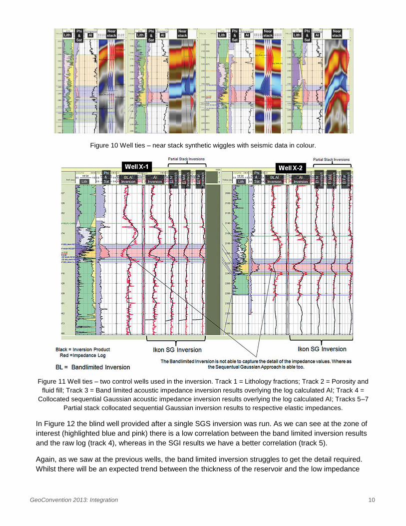
Figure 10 Well ties – near stack synthetic wiggles with seismic data in colour.

Figure 11 Well ties – two control wells used in the inversion. Track 1 = Lithology fractions; Track 2 = Porosity and

fluid fill; Track 3 = Band limited acoustic impedance inversion results overlying the log calculated AI; Track 4 =

Collocated sequential Gaussian acoustic impedance inversion results overlying the log calculated AI; Tracks 5–7

Partial stack collocated sequential Gaussian inversion results to respective elastic impedances.

In Figure 12 the blind well provided after a single SGS inversion was run. As we can see at the zone of

interest (highlighted blue and pink) there is a low correlation between the band limited inversion results

and the raw log (track 4), whereas in the SGI results we have a better correlation (track 5).

Again, as we saw at the previous wells, the band limited inversion struggles to get the detail required.

Whilst there will be an expected trend between the thickness of the reservoir and the low impedance


values, the absolute values of the band limited inversion are not of the same scale as those of the log.

This makes any facies or reservoir characterization based on this inversion directly impossible.

Conversely we see that the SGI values are in an equivalent range (Figure 13).

Once the method (collocated SGI) was agreed and all preparations completed, multiple realizations of

joint stochastic inversions (JSI) were run. In JGI we invert simultaneously – for example to AI and GI.

We use a statistical rock physics model (a cloud transform in this case) made from well log data and

modelled data to ensure that the resulting AI and GI realizations have the same statistical relationship

as the well-log data (Figure 9). Not only does AI have to match with the normal incidence reflectivity,

and GI with the gradient reflectivity seismic, but both the AI and GI profiles need to match satisfactorily

to the well and model-based cloud transform.

All of the JSI results are equi-probable, and statistical analysis can make use of the multiple cubes in a

post processing manner. One approach used here was to invert simultaneously to AI and EI, create

mean cubes of AI and EI, and then apply a Bayesian classification scheme created from pdf maps

extracted from cross plots (Figure 14) to map out reservoir quality types. The end result shows the

results in the form of a ‘Most likely’ or Maximum a-posteriori probability’ cube. Here the classifications

groups are high, mid, and low porosity classes. Alternatively outputs can be probability cubes of high

porosity sand or even gas saturation.

Figure 12: Blind well used for quality assurance. Track 1 = lithology fractions; Track 2 = Porosity and fluid fill;

Track 3 = AVO synthetic; Track 4 = Band limited Acoustic impedance inversion results overlying the log

calculated AI; Track 5 = Collocated sequential Gaussian acoustic impedance inversion results overlying the log

calculated AI; Track 6: Seismic and synthetic along well path.


Figure 13: A comparison of a band limited inversion versus a single sequential Gaussian inversion.


Figure 14: Bayesian classification.

Another approach that was used for comparison was applying a rock physics model to create fluid and

lithology indicators and thus be able to produce a pay indicator. The following equations were used to

map out the resulting property cubes from the mean AI and GI products.

Fluid indicator: ( )

Lithology indicator: (( ) )

Pay = Fluid indicator * Lithology indicator

The rock physics model pay prediction provides a cleaner looking pay than the Bayesian classification

as shown by Figure 15. The transition from pay to non-pay is more gradual rather than at the edges of

the Bayesian classification method, it is more of a sharp transition and appears more noisy.

Figure 15: Pay indicator from a) Rock physics model and b) Bayesian classification.

Conclusions

The forward modelling of the various scenarios gave the interpretation team an understanding of the

effects of various conditions (brine, gas, high porosities, and low porosities). It identified that it would


be possible to separate out the lithology effects and the fluid effects, prevent a misinterpretation, and

provide an insight into where the inversion results and classification would lead.

The data conditioning of partial stacks proved to be an essential part of the workflow, making the

gradient stack a coherent volume rather than a volume dominated by noise. Calibrating the background

AVO seismic signature to the wells meant that the synthetic and seismic responses were aligned in

their properties in and around the reservoir. The ability to optimally condition partial stacks rather than

raw gathers meant that the time and cost were greatly reduced, giving operational flexibility.

A comparison of a conventional band limited inversion versus the stochastic inversion highlighted the

weakness of the band limited inversion to capture the detail required due to resolution issues.

Stochastic inversions are an integrated modelling method and are capable of capturing or including

very high resolution detail from the well. By using a relatively coarse sample rate of 2 ms we were able

to prudently predict below standard seismic resolution, and therefore the seismic data drove the

inversion rather than geostatistics. Whilst there were discrepancies between the realizations, a

consistency in general supported a strong inversion result and a common answer. Acoustic and

gradient impedance were fundamental in the reservoir characterization, and the elastic impedance

acted as a good QC of the inversion prediction and results.

The Bayesian classification and rock physics model calibrated methods both showed similar results in

predicting pay vs. non-pay areas, with the rock physics model providing a possibly more refined final

result. The overall method shows a robust and coherent approach to understanding and predicting the

reservoir characteristics. It also allowed us to gain confidence in predictions of proximal prospects. The

use of the stochastic inversion and Bayesian classification and rock physics models to constrain and

calibrate the inversions gives the results enhanced meaning in terms of reservoir properties.

The rock physics to reservoir workflow produces a sophisticated high resolution static model which

integrates all seismic and well data into one workflow from the basic interpretation through to dynamic

modelling.

References

E. Efthymiou, Morris, H. Kemper, M. and Kerr, J.D. [2010] Seismic Data Conditioning of Partial Stacks for AVO - Using Well

Offset Amplitude Balancing. 72nd EAGE Conference & Exhibition, Poster Presentation.

Doyen. P. [2007] Seismic Reservoir Characterization: An Earth Modelling Perspective. EAGE Publication.

Lancaster, A. and Whitcombe, D. [2000] Fast-track ‘coloured’ inversion. 70th Expanded Abstracts, 19, 1572.

rock physics and reservoir characterization of a calcitic ... · geoconvention 201 3: integration 1...

Documents