rock fall engineering: development and calibration …
TRANSCRIPT

ROCK FALL ENGINEERING: DEVELOPMENT AND CALIBRATION OF AN IMPROVED MODEL FOR ANALYSIS OF ROCK FALL HAZARDS ON HIGHWAYS AND RAILWAYS
by
Duncan C. Wyllie
A THESIS SUBMITTED IN PARTIAL FULFILLMENT OF THE REQUIREMENTS FOR THE DEGREE OF
DOCTOR OF PHILOSOPHY
in
The Faculty of Graduate and Postdoctoral Studies
(Geological Engineering)
THE UNIVERSITY OF BRITISH COLUMBIA
(Vancouver)
June 2014
© Duncan C. Wyllie, 2014

ii
ii
Abstract
My research on rock falls over the last five years is an extension of my 45 year professional
career that has included a wide variety of rock fall projects. This experience has provided me
with an excellent understanding of rock fall behavior; the objective of my research has been to
apply this to developing improvements in rock fall modeling methods and design of rock fall
containment structures. My research to meet these objectives has involved the following:
Case studies – details of rock fall behavior at six locations with varied topography and geology
are presented, and the results have been used to verify the application of impact mechanics
theory to rock falls, and to calibrate modeling programs.
Rock fall trajectories and velocities – the application of Newtonian mechanics to rock fall
trajectories and velocities is described, and results compared with actual translational and
angular velocities, and trajectory heights.
Impact mechanics – the application of theoretical impact mechanics to rock fall impacts is
discussed in terms of [normal impulse – relative velocity] diagrams for rough, rotating bodies,
and equations relating impact and restitution velocities and angles.
Coefficient of restitution – it is shown that the normal coefficient of restitution defined by the
normal final and impact velocities is related primarily to impact angle rather than slope material
properties. Furthermore, for shallow impact angles less than about 20 degrees, the normal
coefficient of restitution can be greater than 1.0.
Energy changes – energy is lost during impact and gained during trajectories. Equations for
energy changes are developed, as well as diagrams showing values of changing potential, kinetic
and angular energies during rock falls.
Rock fall modeling – results of rock fall modeling using the RocScience program RocFall 4.0 for
five case studies are presented; the applicable input parameters are listed.
Design of protection structures –impact mechanics and scale model tests of protection nets
show that these structures can be designed to redirect rather than stop rock falls, and to absorb
energy uniformly during impact. These properties mean that only a portion of the impact
energy is absorbed by the net and that forces induced in the net are minimized.

iii
Preface
This dissertation is original, independent work of the author, Duncan C. Wyllie.
The work includes six case studies. Field data for two of the case studies (Tornado and Mount
Stephen) is new data that was collected by the author specifically for this research. The third
case study (asphalt) is a rock fall that was carefully documented for a project; permission to use
this data for the research has been obtained from the client. The other three studies are
published data: Kreuger Quarry rock fall tests in Oregon, Uma-gun Doi-cho rock fall test site in
Ehime Prefecture, Japan and laboratory tests at Kanazawa University, Japan. The Oregon case
study is public domain data, while permission to use the Japanese data has been obtained from
the authors.
Portions of the dissertation will be published in 2014 as follows:
Calibration of Rock Fall Parameters, to be published in the International Journal of rock
Mechanics and Mining Sciences; the material for this paper forms part of Chapters 2
and 4 of the thesis.
Rock Fall Engineering, a textbook to be published by Taylor and Francis, in London, U.K.;
the book contains Chapters 2 to 7 of the thesis and the appendices, and four additional
chapters.
Duncan C. Wyllie, P. Eng. Dr. Erik Eberhardt, Ph.D., P. Eng.
January 2014

iv
Table of Contents
ABSTRACT ...................................................................................................................................... ii
PREFACE ........................................................................................................................................ iii
TABLE OF CONTENTS .................................................................................................................... iv
LIST OF TABLES ........................................................................................................................... viii
LIST OF FIGURES ........................................................................................................................... ix
LIST OF SYMBOLS ......................................................................................................................... xv
1 INTRODUCTION – OBJECTIVES AND METHODOLOGY ...................................................... 1
1.1 Rock falls – causes and consequences ................................................................ 1
1.2 Background to rock fall research program .......................................................... 3
1.3 Objectives of research ......................................................................................... 5
1.3.1 Objective #1 – Document rock fall events ............................................. 6
1.3.2 Objective #2 – Develop applications of impact mechanics to rock fall .. 6
1.3.3 Objective #3 – Calibrate of rock fall modeling parameters.................... 6
1.3.4 Objective #4 – Test improved rock fall protection structures ............... 7
1.4 Methodology ....................................................................................................... 7
1.4.1 1 – Documentation of rock fall events ................................................... 7
1.4.2 2 – Trajectories and translational/rotational velocities ......................... 8
1.4.3 3 – Application of impact mechanics to rock falls .................................. 8
1.4.4 4 – Rock fall modeling ............................................................................ 9
1.4.5 5 – Development and testing of attenuator-type rock fall fences ......... 9
1.4.6 Conclusions ........................................................................................... 10
2 DOCUMENTATION OF ROCK FALL EVENTS ..................................................................... 11
2.1 Impacts on rock slopes ...................................................................................... 12
2.1.1 Mt. Stephen, Canada – 2000 m high rock slope................................... 13
2.1.2 Kreuger Quarry, Oregon – rock fall test site ........................................ 18
2.1.3 Ehime, Japan – rock fall test site .......................................................... 20
2.2 Impacts on talus and colluvium slopes .............................................................. 23
2.2.1 Ehime, Japan – rock fall tests on talus ................................................. 23
2.2.2 Tornado Mountain – rock falls on colluvium ....................................... 24
2.3 Impact on asphalt .............................................................................................. 30
2.4 Impact with concrete ........................................................................................ 32
2.5 Summary of case study results .......................................................................... 32
3 ROCK FALL VELOCITIES AND TRAJECTORIES ................................................................... 35
3.1 Trajectory calculations ...................................................................................... 35
3.1.1 Trajectory equation .............................................................................. 36

v
3.1.2 Nomenclature – trajectories and impacts ............................................ 38
3.1.3 Rock fall trajectories ............................................................................. 38
3.1.4 Trajectory height and length ................................................................ 41
3.1.5 Field trajectory heights......................................................................... 44
3.2 Rock fall velocities ............................................................................................. 47
3.2.1 Field velocity measurements ............................................................... 47
3.2.2 Effect of friction and slope angle on velocity ....................................... 48
3.3 Variation of trajectories with restitution angle ................................................. 51
3.3.1 Calculated trajectories for varying restitution angles (θ0) ................... 51
3.3.2 Field values of restitution angles (θ0) ................................................... 52
3.4 Angular velocity ................................................................................................. 56
3.4.1 Field measurements of angular velocity .............................................. 56
3.4.2 Relationship between trajectories and angular velocity ...................... 59
3.5 Field observations of rock fall trajectories ........................................................ 59
3.5.1 Rock falls down gullies ......................................................................... 60
3.5.2 Run-out distance .................................................................................. 61
3.5.3 Dispersion in run-out area.................................................................... 62
4 IMPACT MECHANICS ...................................................................................................... 63
4.1 Principles of rigid body impact .......................................................................... 63
4.1.1 Rigid body impact ................................................................................. 63
4.1.2 Kinetics of rigid bodies ......................................................................... 65
4.2 Forces and impulses generated during collinear impact .................................. 65
4.3 Energy changes during impact .......................................................................... 67
4.4 Coefficient of restitution ................................................................................... 69
4.5 For frictional angular velocity changes during impact, for rough surface ........ 73
4.6 Impact behaviour for rough, rotating body ...................................................... 76
4.6.1 Impulse calculations ............................................................................. 77
4.6.2 Final velocities for rock fall impacts ..................................................... 79
4.6.3 Example of impact mechanics calculation ........................................... 82
4.6.4 Effect of angular velocity on trajectories ............................................. 83
4.7 Calculated vs. actual restitution velocities ........................................................ 85
5 COEFFICIENT OF RESTITUTION ....................................................................................... 87
5.1 Newton’s coefficient of restitution ................................................................... 88
5.2 Normal coefficient of restitution ....................................................................... 89
5.2.1 Theoretical relationship between impact angle and normal coefficient
of restitution ...................................................................................................... 90
5.2.2 Field data showing relationship between impact angle and normal
coefficient of restitution .................................................................................... 95
5.2.3 Application of [θi – eN] relationship to rock fall modeling .................... 98
5.3 Tangential coefficient of restitution and friction .............................................. 99
5.3.1 Field values of tangential coefficient of restitution ........................... 100
5.3.2 Application of eT to rock fall modeling ............................................... 102

vi
6 ENERGY CHANGES DURING IMPACTS AND TRAJECTORIES .......................................... 104
6.1 Impact mechanics theory and kinetic energy changes ................................... 105
6.1.1 Kinetic energy changes for normal impact, non-rotating body ......... 105
6.1.2 Kinetic energy changes for inclined impact, rotating body ................ 110
6.2 Rotational energy gains/losses ........................................................................ 116
6.3 Total energy losses .......................................................................................... 117
6.4 Energy loss diagrams ....................................................................................... 118
6.4.1 Energy partition diagram for potential, kinetic and rotational energies
119
6.4.2 Energy head ........................................................................................ 121
6.5 Loss of mass during impact ............................................................................. 122
6.6 Effect of trees on energy losses ...................................................................... 127
7 ROCK FALL MODELING ................................................................................................. 131
7.1 Spreadsheet calculations ................................................................................. 132
7.2 Terrain model – two dimensional v. three dimensional analysis .................... 133
7.3 Modeling methods – lumped mass ................................................................. 134
7.3.1 Rock fall mass and dimensions ........................................................... 134
7.3.2 Slope definition parameters ............................................................... 135
7.3.3 Rock fall seeder .................................................................................. 135
7.3.4 Normal coefficient of restitution ........................................................ 136
7.3.5 Tangential coefficient of restitution and friction ............................... 137
7.3.6 Surface roughness .............................................................................. 138
7.3.7 Rotational velocity .............................................................................. 139
7.3.8 Probabilistic analysis .......................................................................... 140
7.3.9 Data sampling points .......................................................................... 140
7.4 Modeling methods – discrete element model (DEM) ..................................... 141
7.5 Modeling results of case studies ..................................................................... 141
7.5.1 Rock fall model of Mt. Stephen events .............................................. 141
7.5.2 Rock fall model of Kreuger Quarry, Oregon tests .............................. 145
7.5.3 Rock fall model of Ehime, Japan test site ........................................... 148
7.5.4 Rock fall model of Tornado Mountain events .................................... 152
7.5.5 Rock fall model of asphalt impact event ............................................ 156
7.6 Summary of rock fall simulation results .......................................................... 158
8 DESIGN PRINCIPLES OF ROCK FALL PROTECTION STRUCTURES ................................... 160
8.1 Structure location with respect to impact points ........................................... 160
8.2 Attenuation of rock fall energy in protection structures ................................ 161
8.2.1 Velocity changes during impact with a fence ..................................... 162
8.2.2 Energy changes during impact with a fence ...................................... 166
8.2.3 Energy efficiency of fences ................................................................. 167
8.2.4 Configuration of redirection structures ............................................. 168
8.2.5 Hinges and guy wires .......................................................................... 169
8.3 Minimizing forces in rock fall protection fences ............................................. 171
8.3.1 Time – force behavior of rigid, flexible and stiff structures ............... 171

vii
8.3.2 Energy absorption by rigid, flexible and stiff structures .................... 174
8.4 Design of stiff, attenuator fences .................................................................... 178
8.5 Model testing of protection structures ........................................................... 180
8.5.1 Model testing procedure .................................................................... 180
8.5.2 Model test parameters ....................................................................... 182
8.5.3 Results of model tests ........................................................................ 182
9 CONCLUSIONS AND ON-GOING RESEARCH .................................................................. 187
9.1 Conclusions ...................................................................................................... 187
9.1.1 Case studies of rock fall events and testing sites ............................... 187
9.1.2 Impact mechanics theory ................................................................... 187
9.1.3 Performance of rock fall protection structures .................................. 188
9.2 Future research work ...................................................................................... 190
9.2.1 Additional case studies ....................................................................... 190
9.2.2 Impact mechanics ............................................................................... 190
9.2.3 Protection structures.......................................................................... 190
REFERENCES .............................................................................................................................. 192
APPENDIX A: DOCUMENTATION OF ROCK FALL IMPACTS AT MOUNT STEPHEN ..................... 198
APPENDIX B: IMPACT MECHANICS – NORMAL COEFFICIENT OF RESTITUTION ........................ 204
APPENDIX C: IMPACT MECHANICS – IMPACT OF ROUGH, ROTATING BODIES ......................... 209
C.1 Equations of relative motion ........................................................................... 209
C.2 Equations of planar motion for impact of rough bodies ................................. 213
C.3 Equations of motion for translating and rotating bodies – final velocities ..... 215
APPENDIX D: ENERGY LOSS EQUATIONS ................................................................................... 219
APPENDIX E: CONVERSION FACTORS ........................................................................................ 223
INDEX.................... ..................................................................................................................... 226

viii
List of Tables
Table 2-1: Mt Stephen rock fall site: trajectory S-A-B from 112 m above track ........................... 17
Table 2-2: Oregon impact points from source at crest: 15 m high cut at face angle of 76° ......... 18
Table 2-3: Ehime, Japan rock fall test site: trajectory for concrete cube ...................................... 22
Table 2-4: Tornado Mountain rock fall A trajectory from source, fall height 350 m .................... 26
Table 2-5: Impact on asphalt ......................................................................................................... 31
Table 2-6: Summary of rock properties ......................................................................................... 33
Table 2-7: Summary of coefficients of restitution calculated for rock fall case studies ............... 34
Table 3-1: Values of effective friction coefficient μ´ for characteristics of slope materials ......... 50
Table 4-1: Volume and radius of gyration of common rock fall body shapes ............................... 79
Table 7-1: Summary of input parameters used in RocFall 4.0 to stimulate case study rock falls 159

ix
List of Figures
Figure 1.1: Consequences of rock falls; a) rock fall that blocked highway; b) rock fall that was struck by car .....................................................................................................................................1
Figure 1.2: Typical slope configuration showing the relationship between slope angle and rock fall behavior ......................................................................................................................................3
Figure 2.1: Mt. Stephen rock fall site. a) view of lower one third approximately of rock face with concrete block barrier at base of slope; b) MSE barrier constructed with concrete blocks, compacted rock fill and Geogrid reinforcing strips, with steel mesh fence along top, to contain rock falls and snow avalanches (courtesy Canadian Pacific Railway) ........................................... 14
Figure 2.2: Mt. Stephen – cross section of lower part of slope showing ditch and typical trajectories for falls that impact the barrier.................................................................................. 16
Figure 2.3: Image of rock fall test carried out in Oregon (Pierson et al., 2001) ............................ 19
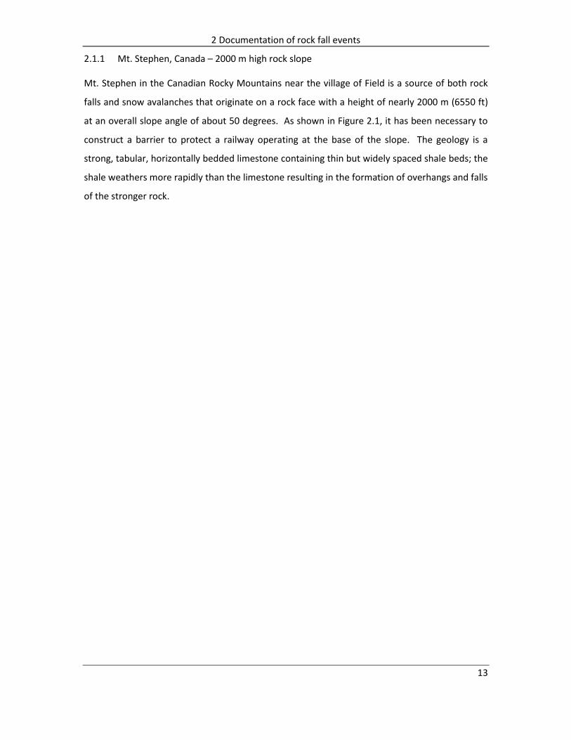
Figure 2.4: Kreuger Quarry, Oregon test site - typical rock fall trajectory and impact points for 15 m high, 76 degree rock face with horizontal ditch ........................................................................ 20
Figure 2.5: Ehime test site in Japan – rock slope with talus deposit at base; concrete cube test block .............................................................................................................................................. 21
Figure 2.6: Ehime test site, Japan – results of rock fall test showing trajectories, and impact and restitution velocities for concrete cube test block; h´ is maximum trajectory height normal to slope, vi, vf are impact and final velocities (Ushiro et al., 2006) ................................................... 23
Figure 2.7: Images of Tornado Mountain rock fall. a) tree with diameter of about 250 mm (9.8 in) sheared by falling rock at a height of about 1.6 m (5.2 ft); fragment of rock broken off main rock fall visible in lower left corner; b) Boulder A, with volume of about 1.4 cu. m (1.8 cu. yd), at slope distance of about 740 m (2,450 ft) from source ........................................................................... 25
Figure 2.8: Tornado Mountain, Boulder A – mapped impact points (total 46) and broken trees
(indicated by arrows ), with detail of velocity components at impact #A26 .............................. 29
Figure 2.9: View of 138 m (450 ft) high slope comprising 58 m (190 ft) high rock slope where rock fall originated, colluvium slope at 42 degrees, and 10 m (33 ft) high cut face above the road .... 30
Figure 2.10: Final trajectory of a rock falling from a height of 136 m (445 ft) and impacting a horizontal asphalt surface ............................................................................................................. 31
Figure 3.1: Examples of impact points visible in the field. a) Distance successive impact points on slope surface (Christchurch, New Zealand 2011 earthquake); b) impact point on tree showing trajectory height (Tornado Mountain, Canada) ............................................................................ 35
Figure 3.2: Definition of trajectory velocity components and directions ..................................... 37
Figure 3.3: Definition of trajectory parameters. a) Velocity nomenclature for trajectories and impacts; b) parameters used in equation (3.4) to calculate rock fall trajectories ........................ 40
Figure 3.4: Trajectory calculations showing rock fall path, impact points, impact velocities and trajectory height and length .......................................................................................................... 43
Figure 3.5: Plot of normal trajectory heights from Ehime test site for spherical and cubic concrete blocks, and blocks of rock (see Figure 2.6 for slope section). (Ushiro et al., 2006) ....... 46

x
Figure 3.6: Range of velocities for Ehime rock fall test site (see Figure 2.6 for slope section) ..... 48
Figure 3.7: Velocity of rock fall on slope dipping at ψs: a) limit equilibrium forces acting on sliding block; b) relationship between free fall height, H and sliding distance, S .................................... 49
Figure 3.8: Trajectories related to restitution angle, θ0: θ0 = 15 degrees and θ0 = 45 degrees .... 52
Figure 3.9: Ranges of values for restitution angle, θ0. a) Tornado Mountain tree impacts (21 points); b) Ehime test site trajectory measurements for spherical, cubic concrete blocks and blocks of rock (Ushiro et al., 2006) ................................................................................................ 55
Figure 3.10: Relationship between angular velocity and fall height for rock falls at Ehime test site, Japan for spherical and cubic concrete blocks, and of blocks of rock (Ushiro et al., 2006) .. 58
Figure 3.11: Effect of attitude of block during impact on angular velocity ................................... 59
Figure 3.12: Mountain slope with three sinuous gullies in which all rock falls are concentrated 61
Figure 4.1: Forces generated at contact point during normal impact .......................................... 64
Figure 4.2: Variation in force F during impact. a) Relationship between force and deformation at the impact point; b) change in force and impulse with time during impact; pc is impulse generated up to time of maximum compression (t = i to t = c); (pf – pc) is impulse generated during restitution phase of impact (t = c to t = f) .......................................................................... 68
Figure 4.3: Example of plastic impact where a rock fall is embedded in a gabion wall ................ 69
Figure 4.4: Relationship between normal impulse pN and changes in tangential and normal velocities vT, vN, and energy during impact; EcN is the kinetic energy absorbed during the compression phase of impact (t = c); (EfN – EcN) is the strain energy recovered during the restitution phase (t = c to t = f) ...................................................................................................... 70
Figure 4.5: Changes in rotational (ω) and slip (vs) velocities during impact, and transition from slip to rolling mode when vs = 0. a) Negative angular velocity: vS = (vT – r · ω); b) positive angular velocity: vS = (vT + r · ω) .................................................................................................................. 75
Figure 4.6: Impact of rough, rotating sphere on a slope in plane motion .................................... 77
Figure 4.7: Diagram of impact showing equations defining impact and restitution velocity vectors ....................................................................................................................................................... 81
Figure 4.8: Example of rock fall impact showing values calculated final (restitution) velocity and angle .............................................................................................................................................. 82
Figure 4.9: Influence of impact angular velocity, ωi on restitution velocity, vf and angle, θf. a) ωi = -15 rad · s-1; b) ωi = -25 rad · s-1; c) ωi = +15 rad · s-1 ............................................................... 84
Figure 4.10: Plot comparing restitution velocities – actual (Chapter 2) and calculated (equations (4.20) to (4.24)) values .................................................................................................................. 86
Figure 5.1: Impacts between successive trajectories showing typical inelastic behavior and loss of energy during impact where second trajectory (on right) is lower than first trajectory; rock falls will always have lower trajectories than those shown (Micheal Maggs, Wikimedia Commons) ..................................................................................................................................... 87
Figure 5.2: Normal impulse-velocity plot showing relationships between changes in normal (N) and tangential (T) velocity components and coefficients of restitution – eN = (vfN/viN) and eT = (vfT/viT) ............................................................................................................................................ 88

xi
Figure 5.3: Isaac Newton's measurement of normal coefficient of restitution using impact of spheres suspended on pendulums ................................................................................................ 89
Figure 5.4: a) Effect of impact angle θi on the normal coefficient of restitution, eN; b) Geometry of collinear and eccentric impacts ................................................................................................. 92
Figure 5.5: Relationship between impact angle θi and normal coefficient of restitution eN with best fit (power) curve for average values of θi and eN each material type ................................... 94
Figure 5.6: Measurement of normal coefficient of restitution for concrete using drop test (hi) to measure rebound height (hf) (Masuya, et al., 2001) ..................................................................... 96
Figure 5.7: Relationship between impact angle θi and the normal coefficient of restitution eN for the rock fall sites described in Chapter 2; total of 58 points for five slope materials................... 97
Figure 5.8: Values for tangential coefficient of restitution eT for 56 impact points at rock fall sites described in Chapter 2 ................................................................................................................ 100
Figure 5.9: Test procedure to measure friction coefficient between block of rock and slope material (Masuya, et al., 2001) ................................................................................................... 102
Figure 6.1: Rock fall that stopped, just before causing serious damage to a building, when it impacted a horizontal surface that absorbed most of the fall energy ........................................ 105
Figure 6.2: Energy changes (normal) during compression and restitution phases of impact. a) Forces generated at contact point during normal impact; b) energy plotted on [force, F – deformation, δ] graph; c) energy changes plotted on [normal impulse, pN – relative velocity, v] graph ............................................................................................................................................ 107
Figure 6.3: Reduction in tangential velocity, vT during impact. a) [pN – v] diagram showing change in vT during impact, and corresponding reduction in energy, ET; b) changes in velocity components ................................................................................................................................. 113
Figure 6.4: Translational and angular velocity components at impact point #A26 for Tornado Mountain rock fall event ............................................................................................................. 115
Figure 6.5: Energy loss diagram for cubic, concrete block with constant mass at Ehime test site, Japan – see Figure 2.6 (Ushiro et al., 2001) ................................................................................. 121
Figure 6.6: Plot of horizontal rock fall distance x against loss of volume ratio, Ω/Ω0 showing ranges of values of λ for data from Mt. Pellegrino and Camaldoli Hills (Nicolla et al., 2009)..... 124
Figure 6.7: Energy partition plot for diminishing mass at the Ehime rock fall test site – cubic concrete block with initial side length 0.6 m (2 ft) ...................................................................... 126
Figure 6.8: Relationship between maximum energy that can be dissipated by six different tree species and the tree diameter, measured at chest height (Dorren and Berger, 2005) .............. 128
Figure 6.9: Impact of a 5 cu. m (6.5 cu. yd) rock fall with kinetic energy of about 200 to 800 kJ (75 to 300 ft tonf) with a 1.1 m (3.6 ft) diameter cedar tree. Rock was stopped and upper part of tree was broken off about 14 m above base (Vancouver Island, near Ucluelet) ........................ 130
Figure 7.1: Rock falls at Mt. Stephen (see section 2.1). a) Simulation of rock falls showing three typical rock fall paths; b) accumulation of falls that impacted fence on top of barrier .............. 132
Figure 7.2: Plot of normal component of impact velocity and scaled normal coefficient of restitution from equation (7.1) ................................................................................................... 137

xii
Figure 7.3: Relationship between slope roughness (ε) and radius of rock fall (r) ....................... 139
Figure 7.4: Simulation of rock falls at Mt. Stephen for three calculated rock trajectories ......... 143
Figure 7.5: Calculated vertical distribution impact points on barrier at Mt. Stephen ................ 144
Figure 7.6: Analysis using RocFall 4.0 of rock falls at Mt. Stephen at barrier, analysis point x = 116.3 m a) translational velocity distribution; b) total energy (KE + RE) distribution................. 145
Figure 7.7: Calculated trajectories for two 580 kg (1,280 lb) rocks at Krueger Quarry rock fall tests on 15 m (50 ft) high cut at a face angle of 76 degrees; refer to Fig 10.3 for first impact and roll out distances ......................................................................................................................... 147
Figure 7.8: Analysis using RocFall 4.0 of rock falls at Krueger Quarry for 15 m (50 ft) high cut at a face angle of 76 degrees, analysis point x = 10 m (33 ft) a) translational velocity distribution; b) total energy (KE + RE) distribution .............................................................................................. 148
Figure 7.9: Calculated trajectory using RocFall 4.0 for a 520 kg (1150 lb) concrete cube at the test site in Ehime Prefecture in Japan ................................................................................................ 150
Figure 7.10: Trajectory height envelope comparison between field results and RocFall 4.0 simulated results for concrete cube at test site in Ehime Prefecture in Japan ........................... 151
Figure 7.11: Analysis using RocFall 4.0 of rock falls at Ehime test side for 42 m (140 ft) high natural slope comprising bedrock (26 m) (85 ft) and talus (16 m) (50 ft) at analysis point x = 52.1 m a) translational velocity distribution; b) total energy (KE + RE) distribution........................... 152
Figure 7.12: Calculated trajectories using RocFall 4.0 for fall A, a 3750 kg (8300 lb) limestone block at Tornado Mountain ......................................................................................................... 154
Figure 7.13: Trajectory height envelope from RocFall 4.0 simulated results for a 3750 kg (8300 lb) limestone block at Tornado Mountain ................................................................................... 154
Figure 7.14: Analysis using RocFall 4.0 of rock falls at Tornado Mountain, block A at analysis point x = 610 m a) translational velocity distribution; b) total energy (KE + RE) distribution ..... 155
Figure 7.15: Calculated trajectories using RocFall 4.0 of a single 500 kg (1,100 lb) rock fall from the crest of the slope and impacting the asphalt road; refer to Figure 2.10 for impact details on asphalt ......................................................................................................................................... 157
Figure 7.16: Analysis using RocFall 4.0 of rock fall impacting asphalt at analysis point x = 140 m a) translational velocity distribution; b) total energy (KE + RE) distribution ................................... 158
Figure 8.1: Tornado Mountain rock fall site – for impact #A43 on 8 m (25 ft) wide bench excavated for the railway, 70 per cent of the impact energy is lost during impact.................... 161
Figure 8.2: Behavior of flexible and rigid structures. a) Flexible steel cable net that stops rock falls by deflection with no plastic deformation of the steel; b) rigid concrete wall shattered by rock fall impact ............................................................................................................................ 162
Figure 8.3: Effect of impact angle with fence on energy absorption. a) Normal impact results in the fence absorbing all impact energy; b) oblique impact results in rock being redirected off the net with partial absorption of impact energy ............................................................................. 163
Figure 8.4: Hanging net installed on steep rock face that redirects rock falls into containment area at base of slope, where cleanout of accumulated rock falls is readily achieved ................ 169

xiii
Figure 8.5: Low friction hinge at base of post allowed the post to deflect, with no damage to the foundation, during an impact that exceeded the service limit states energy (above Shuswap Lake, British Columbia, Canada) .................................................................................................. 170
Figure 8.6: Relationship between time of impact and force generated in rigid, flexible and stiff fences .......................................................................................................................................... 172
Figure 8.7: Plot of duration of impact against rock fall impulse absorbed by fence; curves are developed by integrating [time-force] equations shown in Figure 8.6 to give the area under [time – force] curves ............................................................................................................................. 177
Figure 8.8: [Time – force] -plot for rigid, flexible and stiff structures showing force generated in structure at time taken to absorb impact impulse...................................................................... 178
Figure 8.9: Rock fall trajectories impacting attenuator type fence. Trajectory A – low energy impact close to slope impact point; trajectories B and C – high energy impacts distant from prior impact point ................................................................................................................................ 180
Figure 8.10: a) Baseball pitching machine and b) wave net. ....................................................... 181
Figure 8.11: Configuration of rock fall fence used in model tests. Orientations of hinged posts are defined by angles α and β, measured relative to the normal to the slope ................................. 182
Figure 8.12: Path of deflected projectile after impact with net oriented up-slope (β = +60 degrees). Approximate velocities at ten frame intervals (0.0083 s) during impact shown ....... 183
Figure 8.13: Relationship between energy efficiency and angle β of upper net, for a non-rotating body ............................................................................................................................................. 184
Figure 8.14: Relationship between the duration of impact and change in velocity during impact ..................................................................................................................................................... 185
Figure 8.15: Relationship between duration of impact and the amount of impulse that is absorbed by the fence; compare with Figure 8.7 for stiff structures ......................................... 186
Figure A.1: Plan of Lockblock wall/ fence and slope…………………………………………………….......…....199
Figure A.2: Section #3. a) Cross section view, b) distribution of impact points……………......….... 200
Figure A.3: Section #7. a) Cross section view, b) distribution of impact points………………..........201
Figure A.4: Section #12. a) Cross section view, b) distribution of impact points………………..…....202
Figure A.5: Calculated vertical distribution impact points on barrier at Mt. Stephen………..…....203
Figure B.1: Relationship between normal impulse pN and changes in tangential and normal velocities vT, vN, and energy during impact………………………………………………………………………….....204
Figure C.1: Impact mechanics principles for two dimensional (planar) motion a) forces generated at contact point during normal impact; b) impact of rough, rotating sphere on a slope, v = velocity at center of mass, V = relative velocity at impact point……….....………………......……….....210
Figure C.2: Dimensions of rotating, impacting body defining inertial coefficients for plane motion, rotating about z axis through centre of gravity (+)……………………………………………….......211
Figure C.3: in rotational (ω) and slip (vs) velocities during impact, and transition from slip to rolling mode when vs = 0; for negative angular velocity: vS = (vT – r·ω)……………………………..…....211
Figure C.4: Diagram of impact showing impact and restitution velocity vectors and equations for calculating final velocities……………………………………………………………………………………………………....218

xiv
Figure D.1: Energy changes (normal) during compression and restitution phases of impact. a) Forces generated at contact point during normal impact, with energy changes plotted on [force, F – deformation, δ] graph; b) energy changes plotted on [normal impulse, pN – velocity, v] graph…………………………………………………………………………………………………………………………………......219

xv
List of Symbols
0 Subscript for velocities at the start of trajectory (t = 0) a Constant used in [time – force] relationship for flexible nets; acceleration b Constant used in [time – force] relationship for stiff nets D Diameter of falling rock (m) eN Normal coefficient of restitution eT Tangential coefficient of restitution Ec Energy absorbed during compression phase of impact (J) Ee Energy efficiency for fence design (Ef- Ec) Energy recovered during restitution phase of impact (J) Ei, Ef Impact (i) and restitution (final, f) energies for impact with protection structures
(J) F Force (N) f Subscript for velocities and energies at the completion of impact (t = f) g Gravitational acceleration (m · s-2) H Rock fall height (m) h Trajectory height – vertical (m) h' Trajectory height – normal to slope (m) I Moment of inertia (kg · m2) I´ Tensor defining components of moments of inertia i Subscript for velocities at the moment of impact (t = i); inclination of asperties
(degrees). k Radius of gyration (m) L Side length of cubic block; length of trajectory between impacts; sliding length
of rock falls (m) m Mass of rock fall (kg) m(n) Mass of rock fall at impact point n (kg) m(0) Mass of rock fall at source (kg) N Subscript for the component of velocity normal to the slope n Impact number; gradient of line for [time – force] relationship for rigid
structures p Probability pN Normal impulse (kg · m · s-1) pT Tangential impulse (kg · m · s-1) R Frictional resistance at impact point r Radius of rock fall body (m) s Dimension defining slope roughness (m) T Subscript for the component of velocity tangential to the slope t Time (s) v Relative velocity at contact point (m · s-1) vN Normal component of relative velocity at contact point (m · s-1) vT Tangential component of relative velocity at contact point (m · s-1) Vi Velocity of centre of mass at impact time t = i (m · s-1) Vf Velocity of centre of mass, final or restitution at time t = f (m · s-1) ViN Normal component of impact velocity of centre of mass (m · s-1) ViT Tangential component of impact velocity of centre of mass (m · s-1) VfN Normal component of final velocity of centre of mass (m · s-1)

xvi
VfT Tangential component of final velocity of centre of mass (m · s-1) x Horizontal coordinate (m); exponent in time – force power relationship z Vertical coordinate (m) α Angle of velocity vector relative to positive x-axis (degrees) β1, β2, β3 Inertial coefficients related to rotation of block during impact ε Angle defining slope roughness η Slope resistance factor used in velocity calculations θi Impact angle relative to slope surface (degrees) θf Final or restitution angle relative to slope surface (degrees) κ Slope gradient, trajectory calculations
μ Friction coefficient at impact point μ´ Effective friction coefficient of slope surface σu(r) Uniaxial compressive strength of rock (MPa) φ Friction angle (degrees) ψ Dip angle – slope (s), face (f), plane (p), (degrees) Ω Volume of rock fall (m3) Ω0 Volume of rock fall at source (m3) ω Angular velocity (rad · s-1)

1 Introduction – objectives and methodology
1 1
1 Introduction – objectives and methodology
1.1 Rock falls – causes and consequences
In mountainous terrain, infrastructure such as highways, railways and power generation
facilities, as well as houses and apartment buildings, may be subject to rock fall hazards that can
result in economic losses due to service interruptions, equipment and structural damage, and
loss of life. Figure 1.1 shows two examples of the consequences of rock falls: a) a fall with a
volume of about 80 cu. m from a height of 350 m that shattered an unreinforced concrete wall
and caused severe traffic delays; b) a fall with dimensions of about 150 mm that bounced on the
asphalt and then was struck by a car with the rock passing through the windshield.
Figure 1.1: Consequences of rock falls; a) rock fall that blocked highway; b) rock fall that was struck by car
1 Introduction – objectives and methodology
2
It is well established that rock fall hazards are particularly severe in areas with heavy
precipitation, frequent freeze-thaw cycles (Hungr and Hazzard, 1999; Peckover, 1975; TRB,
1996). These climatic conditions exist, for example, in the Alps, on the west coast of North
America and in Japan. In contrast, in Hong Kong, where temperatures are more mild but intense
rainfall events occur, rock fall hazards can also be severe because of the high population density
(Chau et al., 2003).
Another cause of rock falls are ground motions caused by seismic events (Harp and Jibson, 1995;
Harp et al., 2003). Although rock falls due to earthquakes only occur in seismic-prone zones and
these events are much less frequent than rock falls induced by weathering, the consequence of
earthquake induced events can be widespread and severe as shown by the extensive damage
caused by the 2008 Christchurch earthquake in New Zealand (Dellow, et al., 2011).
As a consequence of these damaging effects of rock falls, and my experience in this field over
the past 40 years, I decided to undertake the research discussed in this thesis. The work was
carried out between 2009 and 2013 with the objectives of understanding rock fall behavior in
detail, and developing methods to improve the design and construction of protection structures.
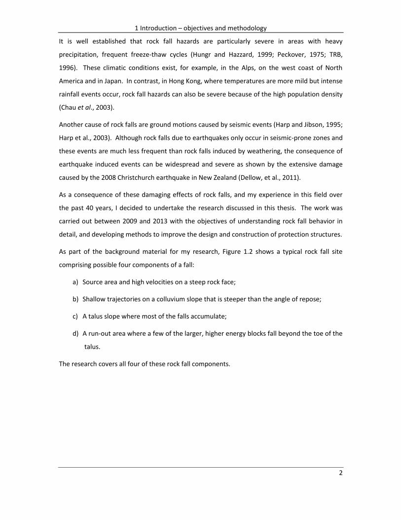
As part of the background material for my research, Figure 1.2 shows a typical rock fall site
comprising possible four components of a fall:
a) Source area and high velocities on a steep rock face;
b) Shallow trajectories on a colluvium slope that is steeper than the angle of repose;
c) A talus slope where most of the falls accumulate;
d) A run-out area where a few of the larger, higher energy blocks fall beyond the toe of the
talus.
The research covers all four of these rock fall components.
1 Introduction – objectives and methodology
3
Figure 1.2: Typical slope configuration showing the relationship between slope angle and rock fall behavior
1.2 Background to rock fall research program
I had my first experience with rock falls in 1968 when working as an underground miner in
Broken Hill, Australia where I was hit by a fall from the “back” (roof) of a development “drive”
(tunnel). Fortunately, my injuries had no lasting effect, and I learnt the significant benefits of
“barring down” (removing loose rock).
My next rock fall experience was in Canada in March 1974, nearly 40 years ago, when a rock fall
caused the derailment of a freight train, with fatal consequences. I was involved in the design
and construction of the remediation work for this incident and this was the start of my
professional career in the field of rock slope engineering for civil engineering projects.
Since 1974 I have been involved in many hundreds of other rock fall projects, mainly in western
Canada, but also in the United States from Alaska to New Jersey, and in Peru, New Zealand,

1 Introduction – objectives and methodology
4
Hong Kong, Greece and Turkey. These projects have involved the investigation, design,
construction and maintenance of remedial measures that have provided me with extensive
experience on the actual behavior of rock falls.
In the 1970’s and 1980’s the only rock fall protection methods available were a simple, but
reliable ditch design chart developed from field tests (Ritchie, 1963), and double twist draped
wire mesh and gabions (rock filled wire baskets) produced by the Maccaferri company in Italy.
Another development in the 1970’s was a rock fall modeling program that was used to examine
rock fall behavior at Hells Gate in the Fraser Canyon, British Columbia; this was probably one of
the first modeling programs (Piteau, 1980).
In the late 1980’s and early 1990’s two significant developments occurred that resulted in a
rapid expansion in the availability in north America of reliable rock fall protection measures.
The first development was the up-grading of Interstate Highway I-70 west of Denver, Colorado
through Glenwood Canyon. One of the project requirements was the retention of the aesthetics
of the canyon by avoiding the excavation of high cuts and wide ditches to contain rock falls.
Because of the significant rock fall hazards from the natural mountain slopes in the canyon, a
comprehensive research program was initiated to develop alternate protection measures to
ditches. The research resulted in the development of mechanically stabilized earth (MSE) rock
fall barriers, attenuator-type structures and Flexpost fences (Barrett and Pfeiffer, 1989; Barrett
and White, 1991; Hearn, 1991). Another development in Colorado at this time was the rock fall
modeling program CRSP (Colorado Rockfall Simulation Program) that was calibrated against
some of the rock fall tests used to evaluate the rock fall protection structures (Pfeiffer and
Bowen, 1989). CRSP has undergone several up-grades and continues to be widely used today. I
have visited Glenwood Canyon and worked with members of CODOT who were responsible for
the research.
The second significant development of the 1980’s was the introduction in North America by
Geobrugg of Switzerland of rock fall fences fabricated with woven wire mesh. One of their early
products was tested in California that demonstrated the viability of using these types of
structures to provide protection against rock falls (Smith and Duffy, 1990). The woven cable
nets have now been replaced by more effective Ringnets, and several other companies (Trumer,
Maccaferri) supply comparable products. I have been involved with several dozen projects using

1 Introduction – objectives and methodology
5
a variety of rock fall fences, and am working with Geobrugg to develop improved protection
products.
I have also been involved for many years with the activities of the Transportation Research
Board (TRB) in Washington, DC that has an active committee on rock fall research. It was
through the TRB that I became acquainted with rock fall mitigation in Japan, and the work of Dr.
Yoshida and Dr. Masuya of Kanazawa University, and Mr. Toshimitsu Nomura of Protec
Engineering in Niigata. I have visited Japan several times to study their approach to rock fall
mitigation. Of particular interest is their work on reinforced concrete rock fall sheds that
incorporate flexible, energy absorbing features (Yoshida et al., 2007). I have also had access to
the results of some of their rock fall testing as described in Chapter 2.
In summary, developments over the last 25 years in the fields of both computer modeling and
mitigation products have provided engineers with the ability to design and build protection
structures that have significantly improved public safety from rock fall hazards. I am very
familiar with all these developments, which, together with my experience on numerous rock fall
projects over the last 40 years, comprises the background to my research.
1.3 Objectives of research
As a result of my experience in rock fall mitigation as described in the previous section, I have
made two observations regarding the design and performance of protection structures where I
thought that it would be possible to make improvements. These two observations were:
i. Fence dimensions – the dimensions of fences are determined by calculating likely rock fall
trajectory heights to make sure that few, if any, rocks pass over the fence. I found that
fences designed with commercially available software such as RocFall 4.0 (RocScience, 2012)
and CRSP (2011), were much higher than required to contain more rock falls. That is,
impacts on the fence were occurring in the lower one third to one quarter with virtually no
impacts in the upper two thirds. These observations were made in about 12 fences where
the sources of the rock falls were at height of up to 250 m, and many hundreds of impacts
had occurred. This clearly demonstrated that the simulation programs were calculating
trajectories that were significantly higher than reality, and that fences were higher, and
more expensive, than required.
ii. Impact energy absorption of protection structures – in the 1960’s and 1970’s, a number of
rigid concrete walls were constructed for rock fall protection. While these walls were

1 Introduction – objectives and methodology
6
effective in containing small falls because of their steep up-slope faces, they were sometime
shattered by larger falls. The wire rope fences introduced in the 1990’s were much more
effective in containing falls than concrete walls because of their flexibility. However, I
observed that most of the impact energy absorption occurred near the point of maximum
deformation when the flexibility of the fence components had diminished and the forces in
the structure suddenly increased. I considered that stiff structures would absorb impact
energy more uniformly during the entire impact period, resulting in the development of
lower forces in the fence. The construction of stiff fences would require modifications to
the configuration and design of fences.
As a result of these observations, four research objectives were developed as discussed below.
1.3.1 Objective #1 – Document rock fall events
Because it is not possible to precisely model rock falls using impact mechanics theory, my
objective has been to carefully document actual rock fall events and use these data to test
impact mechanics theory and calibrate rock fall simulation programs. The events that have
been documented for this research include three sites in British Columbia where I have collected
unique data on impact locations and trajectory paths, and two cases, one in Oregon (Pierson et
al., 2000) and Japan (Ushiro et al., 1999) where details of rock fall tests have been documented
in the literature.
1.3.2 Objective #2 – Develop applications of impact mechanics to rock fall
Rock falls comprise a series of trajectories each followed by an impact. While trajectories can be
readily calculated from Newtonian mechanics, impact is a more complex process involving a
translating and rotating, rough body making an oblique, non-compliant contact with an irregular
slope. My objective was to make a detailed study of impact mechanics theory as developed by
Goldsmith (Goldsmith, 1960) and Stronge (Stronge, 2000) and adapt this theory to rock fall
impacts. Impact mechanics provides detailed information of changes in translational and
rotational velocities, and energies, that occur during the impact process that can be compared
with the field data.
1.3.3 Objective #3 – Calibrate rock fall modeling parameters
The data obtained from the documented rock fall events together with the theoretical velocity
changes during impact can be used to calibrate rock fall modeling programs. My objective has

1 Introduction – objectives and methodology
7
been to run the commercially available program RocFall 4.0 (RocScience 2012) to determine the
values of the input parameters that are needed to closely simulate the documented rock fall
events. The parameters have been compared to the values predicted by impact mechanics
theory. The program RocFall 4.0 was selected because it is widely used and details of the
modeling algorithms are provided.
1.3.4 Objective #4 – Test improved rock fall protection structures
Impact mechanics theory can be applied to the study of how fences and nets contain rock falls.
That is, rock falls are either stopped or redirected by the structure depending on the impact
geometry. Where the rock is stopped, all the impact energy is absorbed by the fence. However,
where rocks are redirected, and not stopped, by the fence, only a portion of the impact energy
is absorbed with the remainder of the energy being retained in the moving body. My objective
was to carry out both impact mechanics analysis and model tests to investigate the relationship
between the impact geometry and the energy absorption of the fence, and determine if this
could be used to design more energy efficient fences.
1.4 Methodology
Section 1.3 above describes the four objectives of my research. The following is a discussion of
the methods used to meet these objectives.
1.4.1 1 – Documentation of rock fall events
My files contain information of 14 rock fall sites, most of which are projects on which I had
worked, together with events that have been reported in the literature. My plan has been to
select sites where the data on impacts and trajectories was both reliable and detailed so that
calculated impact parameters would also be reliable. Also, it was necessary to select sites with a
wide range of both topographic and geologic properties that would encompass most of the rock
fall conditions that occur in nature. I selected five sites, three of which are my own data and
two from the literature, to be my reference rock fall events, as follows:
i. Tornado Mountain in the east Kootenays of British Columbia;
ii. Mt. Stephen near the village of Field in south eastern British Columbia;
iii. A highway location where an impact on asphalt was documented in detail;
iv. Kreuger Quarry in Oregon where 11,500 rock fall tests were documented in detail;

1 Introduction – objectives and methodology
8
v. Test site in Ehime Prefecture on Shikoku Island in Japan where 100 tests were
conducted on blocks of rock, and concrete spheres and cubes.
For each site, the [x –z] co-ordinates of each impact, and the trajectory impact angle (θ0) were
known or measured. A spreadsheet was then written that calculated at each impact the velocity
components (normal, tangential and vertical, horizontal), as well as the normal and tangential
coefficients of restitution (eN, eT). The spreadsheet also calculated the energy loss at each
impact point and the energy gained during each trajectory.
It is intended that these case studies can be used by others to calibrate rock fall modeling
programs.
This work is described in Chapter 2. In addition, Appendix A provides details of the locations of
466 impacts on the barrier at Mt. Stephen.
1.4.2 2 – Trajectories and translational/rotational velocities
The trajectory phase of rock falls involves the application of Newtonian mechanics to determine
the path of the fall through the air and the change in the translational velocity during the
trajectory. This procedure was used to calculate trajectories for the five reference case studies,
and compare actual and theoretical translational velocities.
With respect to rotational velocity, detailed information on these velocities was available from
the Shikoku test site in Japan. These test results are a useful set of data showing the range of
rotational velocities that occur for rock falls, and the relationship between the size of the body
and its rotational velocity.
This subject is addressed in Chapter 3.
1.4.3 3 – Application of impact mechanics to rock falls
The impact mechanics model used in my research is a co-linear (planar) impact of a rough
(frictional), translating and rotating body of any shape defined by its radius (r) and radius of
gyration (k) impacting a stationary, planar but irregular surface (slope). This is a non-compliant
impact where no interpenetration of the bodies occurs. Appendices B, C and D show the
derivation of equations for the changes in velocity and energy during impact for a spherical
body.

1 Introduction – objectives and methodology
9
I have found that a very valuable means of illustrating the impact process is to use [normal
impulse, pN – relative velocity, v] plots. These plots clearly illustrate the changes in translational
and rotational velocity, and energy that occur during impact, and how the frictional and
compression components of impact can be separated. Impact mechanics also shows the effect
of the impact angle for a rough, rotating body on the restitution velocity, and how the normal
coefficient of restitution eN, can be greater than 1 for shallow angle impacts.
Chapters 4, 5 and 6 discuss respectively the principles of impact mechanics, the coefficients of
restitution eN and eT, and energy changes during impact.
1.4.4 4 – Rock fall modeling
I used the simulation program RocFall 4.0 to model the five reference rock fall events. For each
rock fall, the values of the input parameters required to closely match the actual rock fall events
were determined. I found that minor changes in the values of the impact parameters have a
significant effect on rock fall behavior. For each of the reference cases, the required values of
the input parameters – seeder velocities, normal and tangential coefficients of restitution and
surface roughness - are listed.
I intend that these parameter values will provide a guideline to others using this program on
appropriate values to use to simulate actual rock falls.
The analysis results are discussed in Chapter 7.
1.4.5 5 – Development and testing of attenuator-type rock fall fences
I have used the principles of impact mechanics to examine how rock falls interact with rock fall
fences, and the benefit of having fences redirect rather than stop falls. This is, if a rock fall is
redirected, and not stopped, by the fence then only a portion of the impact energy is absorbed
by the net and the rest is retained in the rock fall. Furthermore, if the fence is “stiff” rather than
highly flexible, energy is absorbed uniformly over the duration of the impact resulting in reduced
forces being induced in the fence.
Stiff structures that redirect rock falls are termed “attenuators”.
The theoretical performance of fences with different stiffnesses when impacted by rock falls is
demonstrated by the use of [force – time] diagrams. In order to test this theoretical
performance, I carried out a series of 1/20 scale model tests of a wire mesh fence to investigate
the effect of impact angle on the performance of attenuator-type protection structures. That is,

1 Introduction – objectives and methodology
10
these structures redirected rather than stopped the impacting body such that the velocity was
attenuated during the time of contact. The tests involved using a baseball pitching machine to
project spherical bodies at the wire mesh models. The motion of the body during contact with
the fence and canopy was captured by a high speed camera running at 1205 frames per second
to record the changes in translational and rotational velocity that occurred during contact.
The translational and angular velocities on the high speed videos were analyzed with ProAnalyst
motion analysis software.
The study of attenuator structures is discussed on Chapter 8.
1.4.6 Conclusions
In Chapter 9 I discuss the conclusions that can be drawn from my research, and what further
work may be carried out to develop the theoretical and applied results.
In summary, the research presented in this thesis is a combination of my 40 years of practical
experience with projects involving rock falls, and the last five years of detailed study of five case
studies, impact mechanics theory and model testing of attenuator-type rock fall protection
structures. My overall objective has been to show that the theory can be applied to rock falls
such that rock fall analysis programs can more closely simulate actual field conditions, and that
the principle of attenuation can be used to design more efficient protection structures.

2 Documentation of rock fall events
11 11
2 Documentation of rock fall events
This chapter documents five rock fall events that encompass many commonly occurring rock fall
conditions. These data are from both natural events where it has been possible to precisely
map impact points and trajectories, and from carefully documented, full-scale rock fall tests.
These case studies are for a variety of slope geometries and fall heights, and for slope materials
comprising rock, colluvium, talus and asphalt. For these sites, the velocity components in
directions normal and parallel to the slope have been calculated from the impact co-ordinates,
and the results have been used to calculate normal and tangential coefficients of restitution,
and the energy losses.
The documented events provide reliable data that can be used to calibrate impact and trajectory
models. Each of the case studies has been modeled using the program RocFall 4.0 (RocScience,
2012) as described in Chapter 7, where values for the input parameters that are required to fit
the calculated trajectories to the field conditions are listed.
Rock falls comprise a series of impacts, each followed by a trajectory and methods of modeling
both impacts and trajectories are required to simulate these events. The basic attributes of
trajectories and impacts are as follows:
Trajectory – rock fall trajectories follow well defined parabolic paths according to Newtonian
mechanics, where three points on the parabola completely define the fall path (Chapter 3). In
calculating trajectories at sites where information on precise impact points and trajectory paths
is not available, it is necessary to select the two end points for each trajectory and to make an
assumption for the angle at which the rock leaves the slope surface. These data have been
obtained from measurements at the fully documented rock fall sites, and from only using
trajectories that are found to be both realistic, and mathematically feasible.
Impact – the theory of impact mechanics (Chapter 4) can model rock falls, but it is necessary to
make simplifying assumptions compared to the actual conditions that occur. Natural conditions
includes irregularly shaped, translating and rotating blocks of rock impacting a slope that may be
comprised of a different material and also be rough and irregular.
In examining velocity changes during impact, it is useful to calculate the changes in normal and
tangential velocity components that occur as the result of deformation and friction at the
contact surface. The changes in the velocity components can be quantified in terms of the

2 Documentation of rock fall events
12
normal (eN) and tangential (eT) coefficients of restitution as defined in the following two
equations:
iN
fN
Nvvelocitynormalimpact
vvelocitynormalfinalenrestitutiooftcoefficienNormal
,
,, (2.1)
iT
fT
Tv,velocitygentaltanimpact
v,velocitygentialtanfinale,nrestitutiooftcoefficienTangential (2.2)
For each documented rock fall site described in this chapter, insets on the impact drawings show
arrows, the lengths and orientations of which are proportional to the velocity vectors. The
notation on the vectors include the subscript “i” referring to values at the moment of impact
(time, t = i), and the subscript “f” refers to values at the end of the impact (time, t = f); the final
velocity is also referred to as the “restitution” velocity. Also, the subscript “N” refers to the
component of the vector normal to the slope and the subscript “T” refers to the component of
the vector tangential to the slope at each impact point. The included angle between the vector
and the slope is shown by the symbol θ, with the same subscript designations for impact and
final angles.
It is also noted that normal impact velocities (-viN) are negative because the positive normal axis
is in the direction out of the slope, and consequentially normal restitution velocities (vfN) are
positive. The positive tangential axis is down slope so all tangential velocities are positive.
This chapter documents actual final velocities and angles measured in the field, while Chapter 3
derives the trajectory equations, and Chapter 4 shows the derivation, based on impact
mechanics theory, of equations defining the final velocities and angles. Section 4.7 compares
the actual and calculated sets of data for the five documented case studies. Each case study
gives the shape, dimensions, mass and radius of gyration of typical blocks of rock. It has been
assumed that the rock fall shapes are either cuboid for falls from low heights, or ellipsoidal
where cubic blocks have had the sharp edges and corners broken off by successive impacts on
the slope.
2.1 Impacts on rock slopes
Data have been analyzed for falls at locations in Canada, the United States and Japan, for slopes
ranging in height from 2000 m to 15 m (6550 to 50 ft). The following is a discussion on falls at
three locations where the falls impacted rock slopes.
2 Documentation of rock fall events
13
2.1.1 Mt. Stephen, Canada – 2000 m high rock slope
Mt. Stephen in the Canadian Rocky Mountains near the village of Field is a source of both rock
falls and snow avalanches that originate on a rock face with a height of nearly 2000 m (6550 ft)
at an overall slope angle of about 50 degrees. As shown in Figure 2.1, it has been necessary to
construct a barrier to protect a railway operating at the base of the slope. The geology is a
strong, tabular, horizontally bedded limestone containing thin but widely spaced shale beds; the
shale weathers more rapidly than the limestone resulting in the formation of overhangs and falls
of the stronger rock.

2 Documentation of rock fall events
14
Figure 2.1: Mt. Stephen rock fall site. a) view of lower third, approximately, of rock face with concrete block barrier at base of slope; b) MSE barrier constructed with concrete blocks, compacted rock fill and Geogrid reinforcing strips, with steel mesh fence along top, to contain rock falls and snow avalanches (courtesy Canadian Pacific Railway)

2 Documentation of rock fall events
15 15
The barrier comprises a mechanically stabilized earth (MSE) wall built with pre-cast concrete
blocks (dimensions 1.5 m long, 0.75 m in section; 5 by 2.5 ft) forming each face, with Geogrid
reinforcement and compacted gravel fill between the walls, and a steel cable fence along the
top of the wall. The total height of the structure is 11.6 m (38 ft). Figure 2.2 shows a typical
section of the lower 120 m (400 ft) of the slope that was generated from an aerial Lidar survey
of the site. Figure 2.2 also shows a range of feasible trajectories of rock falls that impacted the
lower part of the rock slope and were then contained by the barrier.

2 Documentation of rock fall events
16
S
A
B
vi = 29.8 ms-1
viN= -13.0 ms-1
vf = 20.6 ms-1
vfT = 18.1 ms-1
vfN= 9.7 ms-1
eN = 0.75eT = 0.68
ψslope = 41˚
θf= 20˚
viT = 26.8 ms-1
θi = 26˚
Detail of velocity componentsat impact point on rock
-ω
αf = 225°
S
A
B
vi = 29.8 ms-1
viN= -13.0 ms-1
vf = 20.6 ms-1
vfT = 18.1 ms-1
vfN= 9.7 ms-1
eN = 0.75eT = 0.68
ψslope = 41˚
θf= 20˚
viT = 26.8 ms-1
θi = 26˚
Detail of velocity componentsat impact point on rock
-ω
αf = 225°
Figure 2.2: Mt. Stephen – cross section of lower part of slope showing ditch and typical trajectories for falls that impact the barrier

2 Documentation of rock fall events
17
Table 2-1: Mt Stephen rock fall site: trajectory S-A-B from 112 m above track
Impact point from source (n)
Impact Coordinates Trajectory angle,
restitution from
horizontal, x axis (αf)
Slope angle
(above impact point)
s
Coefficients of restitution
Kinetic energy
lost during impact (J)
x co-ordinate
(m)
z co-ordinate, elevation
(m)
Normal coefficient
of restitution,
eN
Tangential coefficient
of restitution,
eT
Trajectory S-A-B
1: Source area
40.00 112.00 -
2: Rock face
60.00 71.50 200.0 41.0 0.75 0.68 -10,270
3: Barrier impact
117.00 8.00 - - - - -
It was possible to identify rock fall impact points on both the steel mesh fence and the concrete
blocks, and to define the co-ordinates of each point relative to one end of the wall. In total, 466
impacts were documented. Analyses of typical trajectories that were mathematically and
physically feasible allowed the impact velocity (vi) and restitution velocity (vf) to be calculated at
each impact point from which the velocity components, and tangential (eT) and normal (eN)
coefficients of restitution were determined. The inset on Figure 2.2 shows the velocity
components at impact point A for trajectory S – A – B. Table 2-1 shows detail of trajectory S – A
– B.
The inset shows that velocities at the point of impact for this height of fall can be as great as 30
m · s-1 (100 ft · s-1). Furthermore, calculation of velocities at the point of impact with the barrier
after trajectories that originate at heights of 70 to 100 m (230 to 330 ft) above the barrier can be
as high as 48 m · s-1 (160 ft · s-1). Velocities of this magnitude are consistent with the height of
the fall and the steepness of the slope.
The impact energies can be calculated from the mass and velocities of the falls. The rocks
tended to break up on impact with the rock slope, and the maximum block dimensions of
ellipsoid shaped blocks at the barrier location are about 300 to 500 mm (12 to 20 in), with
masses in the range of 50 to 150 kg (110 to 330 lb). Based on a typical velocity at the point of
impact with the barrier of about 45 m · s-1 (150 ft · s-1), the impact energies (KE =½ m · v2) are
approximately 60 to 180 kJ (22 to 66 ft tonf). It was found that the unreinforced concrete blocks

2 Documentation of rock fall events
18
forming the face of the MSE wall were readily able to withstand these impacts, with damage
being limited to chips a few millimeters deep.
Analyses of these rock falls using the program RocFall 4.0 are given in Section 7.5.1.
Typical rock fall properties: ellipsoidal block with axes lengths 0.4 m (1.3 ft), 0.4 m (1.3 ft) and
0.2 m (0.7 ft), mass of 44 kg (97 lb) (unit weight of 26 kN · m-3 (165 lbf · ft-3)) and radius of
gyration of 0.13 m (0.43 ft) (see Table 4.1 for ellipsoid properties).
2.1.2 Kreuger Quarry, Oregon – rock fall test site
An extensive rock fall test program was carried out at the Kreuger Quarry in Oregon to
determine the required ditch configurations to contain rock falls on highways (Pierson et al.,
2001). The geometries of the excavated rock cuts included cut heights ranging between 8 m (25
ft) and 24 m (80 ft), face angles ranging between vertical and 45 degrees and ditches inclined at
4H:1V and 6H:1V (towards the slope), and horizontal; in total 11,250 separate rock fall tests
were conducted (see Figure 2.3). For each rock fall, the data collected included the first impact
position in the ditch, and the roll-out distance. The rock at the test site was a strong, blocky
basalt that was excavated with controlled blasting on the design final line to produce a face with
few irregularities.
Table 2-2: Oregon impact points from source at crest: 15 m high cut at face angle of 76°
Impact point from
source (n)
Impact Coordinates Trajectory angle,
restitution from
horizontal, x axis (αf)
Slope angle
(above impact
point) s
Coefficients of restitution Kinetic energy
lost during
impact (J)
x co-ordinate
(m)
z co-ordinate, elevation
(m)
Normal coefficient
of restitution,
eN*
Tangential coefficient
of restitution,
eT*
Crest (1) 0.00 15.00 0
76˚ face (2)
1.50 7.00 225.0 76.0 -2.51 0.59 -14,248
Ditch impact (3)
6.25 0.10 140.0 0.0 0.24 0.55 -56,122
2nd impact (4)
9.00 0.00 - - -

2 Documentation of rock fall events
19
Figure 2.3: Image of rock fall test carried out in Oregon (Pierson et al., 2001)
Figure 2.4 and Table 2-2 show that test results for a 15 m (50 ft) high cut at a face angle of 76
degrees (¼H:1V) with a horizontal ditch. The diagram shows the measured location of the first
impact point in the ditch for the 95th percentile of the test rocks, and the assumed trajectories
for a rock fall from the crest of the cut initially impacting the face and then the ditch. The
second impact point in the ditch is an estimated location based on common rock fall behavior.
The inset on Figure 2.4 shows the calculated velocity components, using the spreadsheet
described in Section 7.1, at the impact point on the cut face, and the values for eT and eN for the
first two impact points. These calculated values show the difference in behavior of rock falls
that impact at a shallow angle (on the rock face) and at a steep angle (in the ditch). That is, for
shallow angle impacts, the normal coefficient is greater than 1, while for steep angle impacts the
normal coefficient is less than 1. These field tests and impact mechanics theory show that eN is
related to the impact angle θi, and that eN is generally greater than 1 when θi is less than about
20 degrees – see Figures 5.5 and 5.7. In contrast, the tangential coefficient is less than 1 for
both impacts and the similar values of eT for the two impacts shown in Figure 2.3 indicate that eT
is a function of the slope material rather than the impact conditions. Coefficients of restitution
are discussed in Chapter 5.
Analyses of these rock falls using the program RocFall 4.0 are given in Section 7.5.2.
2 Documentation of rock fall events
20
Typical rock fall properties: cubic block with side lengths 0.6 m (2 ft), mass of 580 kg (1280 lb)
(unit weight of 26 kN · m-3 (165 lbf · ft-3)) and radius of gyration of 0.245 m (0.80 ft).
ψslope= 76˚ψ
slope = 76
˚
vi = 12.5 m · s-1
viN = -2.9 m · s-1
vf = 10.2 m · s-1
vfT
= 7.2 m · s-1
vfN = 7.2 m · s-1
eN = 2.51eT = 0.59
θf = 45˚
viT
= 12.2 m · s-1
Detail of velocity componentsat impact point on rock face
θi = 13˚
-ω
eN = 0.24eT = 0.55
15 mα0 = 225°
α0 = 140°
Figure 2.4: Kreuger Quarry, Oregon test site - typical rock fall trajectory and impact points for 15 m high, 76 degree rock face with horizontal ditch
2.1.3 Ehime, Japan – rock fall test site
In 2003 a rock fall study was carried out on a 42 m (140 ft) high rock and talus slope at the Uma-
gun Doi-cho test site in Ehime Prefecture on Shikoku Island (Ushiro et al., 2006). The slope
comprised a 26 m (85 ft) high rock slope in horizontally bedded sandstone and mudstone with a
face angle of 44 degrees, above a 16 m (50 ft) high talus slope at angle of 35 degrees (Figure
2.5).

2 Documentation of rock fall events
21
Figure 2.5: Ehime test site in Japan – rock slope with talus deposit at base; concrete cube test block

2 Documentation of rock fall events
21 22
Table 2-3: Ehime, Japan rock fall test site: trajectory for concrete cube
Impact point from
source (n)
Impact Coordinates Trajectory angle,
restitution from
horizontal, x axis (αf)
Slope angle
(above impact point)
s
Coefficients of restitution Kinetic
energy lost during
impact (J)
x co-ordinate
(m)
z co-ordinate, elevation
(m)
Normal coefficient
of restitution,
eN
Tangential coefficient
of restitution,
eT
0 – source 0.00 45.00
1 – rock 1.00 44.00 181.0 45.0 0.64 1.01 -1,851
2 – rock 3.00 42.50 205.0 36.9 0.89 0.95 -1,263
3 – rock 6.00 39.70 198.0 43.0 1.71 0.49 -17,403
4 – rock 12.00 31.75 209.7 53.0 0.34 0.94 -8,303
5 – rock 15.00 29.67 189.7 34.7 4.58 0.58 -30,832
6 – talus 28.00 18.23 209.1 41.3 0.22 0.73 -45,806
7 – talus 31.00 16.19 185.6 34.2 5.47 0.71 -17,642
8 – talus 49.00 2.57 184.5 37.1 0.00 0.00 -25,873
9 – stop 53.00 2.00 -148,973
The test involved both natural boulders, and spherical and cubic concrete blocks containing
embedded three dimensional accelerometers and a data acquisition system recording data at a
frequency of 1/2000 seconds. The instrumentation together with high speed cameras, gave the
precise location, and translational and rotational velocities over the full extent of the fall path.
Figure 2.6 shows the impact points and trajectories of a typical test of a concrete cube, together
with the impact and final velocities, vi and vf and the maximum trajectory height h´ measured
normal to the slope (see also Figure 3.5).
Also shown on Figure 2.6 are the calculated velocity components and the values for eN and eT at
impact point #3 on rock, and the eN and eT values for impact points # 6 and #7 on talus. Table 2-
3 shows detail of rock fall trajectory for a concrete cube. For the rock impact, the value for eN is
greater than 1, and has a similar value to that for the Oregon test for the shallow impact angle
point on the steep rock face. At both the Oregon and Ehime test sites, eN values greater than 1
occurred for shallow angle impacts where the impact angles (θi) were small (13 and 12 degrees
respectively).
Analyses of these rock falls using the program RocFall 4.0 are given in Section 7.5.3.
Typical rock fall properties: cubic concrete block with side lengths of 0.6 m (2 ft), mass of 520 kg
(1,150 lb) (unit weight of 24 kN · m-3 (150 lbf · ft-3)) and radius of gyration of 0.245 m (0.80 ft).

2 Documentation of rock fall events
23
Impact #6eN = 0.22eT = 0.73
Impact #7eN = 5.48eT = 0.71
ViVi
ViVi
ViVi
ViVi
ViVi
ViVi
ViVi
h’=0.
27m
h’=0.
98m
h’=0
.27m
h’=0
.09m
h’=1.7
4m
h’=0
.08m
h’=2
.46m
Impact #6eN = 0.22eT = 0.73
Impact #7eN = 5.48eT = 0.71
ViVi
ViVi
ViVi
ViVi
ViVi
ViVi
ViVi
h’=0.
27m
h’=0.
98m
h’=0
.27m
h’=0
.09m
h’=1.7
4m
h’=0
.08m
h’=2
.46m
Impact #6eN = 0.22eT = 0.73
Impact #7eN = 5.48eT = 0.71
ViVi
ViVi
ViVi
ViVi
ViVi
ViVi
ViVi
h’=0.
27m
h’=0.
98m
h’=0
.27m
h’=0
.09m
h’=1.7
4m
h’=0
.08m
h’=2
.46m
viN = -1.9 m · s-1
vf = 5.7 m · s-1
vfT
= 4.7 m · s-1
vfN = 3.3 m · s-1
eN = 1.70eT = 0.49
ψslope = 43˚
θf = 35˚
viT
= 9.5 m · s-1
θi = 12˚
Detail of velocity componentsat impact point #3 on rock
vi = 9.7 m · s-1
-ω
viN = -1.9 m · s-1
vf = 5.7 m · s-1
vfT
= 4.7 m · s-1
vfN = 3.3 m · s-1
eN = 1.70eT = 0.49
ψslope = 43˚
θf = 35˚
viT
= 9.5 m · s-1
θi = 12˚
Detail of velocity componentsat impact point #3 on rock
vi = 9.7 m · s-1
-ω
αf = 185.6°
Figure 2.6: Ehime test site, Japan – results of rock fall test showing trajectories, and impact and restitution velocities for concrete cube test block; h´ is maximum trajectory height normal to slope, vi, vf are impact and final velocities (Ushiro et al., 2006)
2.2 Impacts on talus and colluvium slopes
Information of impacts on talus and colluvium have been obtained from the Ehime test site in
Japan (Figure 2.6), and from two rock falls on Tornado Mountain in south-east British Columbia,
Canada (Figure 2.8).
2.2.1 Ehime, Japan – rock fall tests on talus
The calculated eN and eT values for impact #6 at Ehime on talus are shown on Figure 2.6. It is of
interest that the eT values of #6 and #7 impacts are nearly identical, while the eN values are very
different; the trajectory after impact #6 barely leaves the slope surface, while the trajectory
after impact #7 is the longest and highest of the rock fall. The difference in the trajectories is
probably due to a combination of slope roughness and the attitude of the block as it impacted
the surface. The eN value of 5.48 at impact point #7 is a reliable, measured value that is a
significantly higher than other calculated values at this site.

2 Documentation of rock fall events
24
2.2.2 Tornado Mountain – rock falls on colluvium
The Tornado Mountain site comprises a 50 m (165 ft) high rock face in very strong, blocky
limestone, above a colluvium slope at an angle varying from 35 degrees on the upper slope in
talus to 22 degrees on the lower slope (Figures 2.7 and 2.8). The colluvium is a mixture of gravel
and soil forming a uniform slope with no significant irregularities, and no previous rock falls. The
slope is sparsely vegetated with pine trees having diameters ranging from about 300 to 500 mm
(12 to 20 in).

2 Documentation of rock fall events
25
Figure 2.7: Images of Tornado Mountain rock fall. a) tree with diameter of about 250 mm (9.8 in) sheared by a falling rock at a height of about 1.6 m (5.2 ft); fragment of rock broken off main rock fall visible in lower left corner; b) Boulder A, with volume of about 1.4 cu. m (1.8 cu. yd), at slope distance of about 740 m (2,450 ft) from source

2 Documentation of rock fall events
26
Table 2-4: Tornado Mountain rock fall A trajectory from source, fall height 350 m
Impact point from
source
Impact Coordinates Trajectory angle,
restitution from
horizontal, x axis (αf)
Slope angle
(above impact point)
s
Coefficients of restitution
Kinetic energy
lost during impact (J)
x co-ordinate
(m)
z co-ordinate, elevation
(m)
Normal coefficient
of restitution,
eN
Tangential coefficient
of restitution,
eT
A - source 0.00 350.00
B - rock 8.00 316.00 213.0 76.7 0.24 0.97 -597,368
C - rock 28.00 295.00 205.0 46.4 0.98 0.74 -636,093
D - talus 48.00 280.00 200.0 36.9 1.12 0.84 -383,565
E 72.00 265.00 185.0 32.0 1.19 0.74 -649,674
1 98.00 255.45 167.6 20.2 1.35 0.35 -968,096
2 117.70 244.60 176.2 28.8 0.78 0.53 -428,292
3 132.60 236.15 177.0 29.6 0.88 0.53 -346,394
4 144.60 229.50 176.4 29.0 1.11 0.60 -227,818
5 158.80 221.05 168.0 30.8 1.23 0.52 -291,750
6 176.60 210.90 177.1 29.7 0.82 0.60 -349,399
7 192.20 202.45 175.8 28.4 0.82 0.48 -396,086
8 202.40 197.10 175.1 27.7 1.29 0.72 -119,311
9 218.70 188.05 176.4 29.0 0.63 0.41 -458,078
10 225.70 184.40 174.9 27.5 1.50 0.79 -42,725
11 240.20 176.05 177.3 29.9 0.90 0.60 -294,735
12 253.30 169.30 174.7 27.3 1.26 0.68 -188,389
13 272.00 159.25 175.7 28.3 0.68 0.44 -498,765
14 281.20 154.60 174.2 26.8 1.10 0.62 -163,044
15 291.60 149.15 175.1 27.7 1.00 0.54 -218,672
16 301.70 143.10 178.3 30.9 0.99 0.62 -195,226
17 312.60 136.75 177.6 30.2 1.46 0.79 -80,514
18 335.00 123.10 178.8 31.4 0.85 0.48 -585,150
19 351.60 112.65 179.6 32.2 1.02 0.65 -312,023
20 370.40 102.20 194.5 29.1 0.59 0.85 -218,275
21 383.50 95.25 175.3 27.9 1.44 0.44 -542,278
22 395.60 89.00 189.0 27.3 0.72 0.60 -259,761
23 416.40 77.90 171.0 33.4 1.36 0.57 -200,941
24 427.20 72.65 173.3 25.9 0.94 0.65 -179,329
25 437.70 67.90 171.7 24.3 0.89 0.53 -224,677
26 445.60 64.25 142.6 24.8 1.29 0.27 -179,883
27 452.10 61.20 172.5 25.1 0.89 1.03 -6,012
28 463.00 56.55 158.0 23.1 1.03 0.42 -248,912
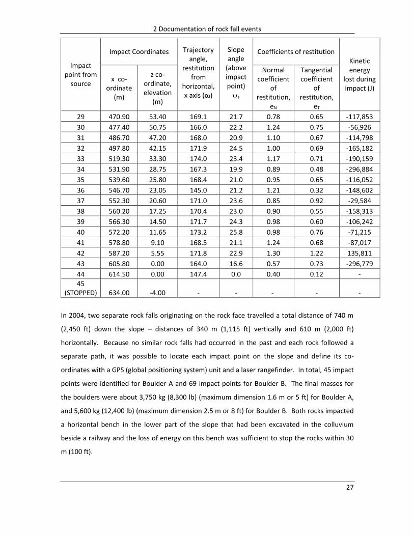
2 Documentation of rock fall events
27
Impact point from
source
Impact Coordinates Trajectory angle,
restitution from
horizontal, x axis (αf)
Slope angle
(above impact point)
s
Coefficients of restitution Kinetic energy
lost during impact (J)
x co-ordinate
(m)
z co-ordinate, elevation
(m)
Normal coefficient
of restitution,
eN
Tangential coefficient
of restitution,
eT
29 470.90 53.40 169.1 21.7 0.78 0.65 -117,853
30 477.40 50.75 166.0 22.2 1.24 0.75 -56,926
31 486.70 47.20 168.0 20.9 1.10 0.67 -114,798
32 497.80 42.15 171.9 24.5 1.00 0.69 -165,182
33 519.30 33.30 174.0 23.4 1.17 0.71 -190,159
34 531.90 28.75 167.3 19.9 0.89 0.48 -296,884
35 539.60 25.80 168.4 21.0 0.95 0.65 -116,052
36 546.70 23.05 145.0 21.2 1.21 0.32 -148,602
37 552.30 20.60 171.0 23.6 0.85 0.92 -29,584
38 560.20 17.25 170.4 23.0 0.90 0.55 -158,313
39 566.30 14.50 171.7 24.3 0.98 0.60 -106,242
40 572.20 11.65 173.2 25.8 0.98 0.76 -71,215
41 578.80 9.10 168.5 21.1 1.24 0.68 -87,017
42 587.20 5.55 171.8 22.9 1.30 1.22 135,811
43 605.80 0.00 164.0 16.6 0.57 0.73 -296,779
44 614.50 0.00 147.4 0.0 0.40 0.12 -
45 (STOPPED) 634.00 -4.00 - - - - -
In 2004, two separate rock falls originating on the rock face travelled a total distance of 740 m
(2,450 ft) down the slope – distances of 340 m (1,115 ft) vertically and 610 m (2,000 ft)
horizontally. Because no similar rock falls had occurred in the past and each rock followed a
separate path, it was possible to locate each impact point on the slope and define its co-
ordinates with a GPS (global positioning system) unit and a laser rangefinder. In total, 45 impact
points were identified for Boulder A and 69 impact points for Boulder B. The final masses for
the boulders were about 3,750 kg (8,300 lb) (maximum dimension 1.6 m or 5 ft) for Boulder A,
and 5,600 kg (12,400 lb) (maximum dimension 2.5 m or 8 ft) for Boulder B. Both rocks impacted
a horizontal bench in the lower part of the slope that had been excavated in the colluvium
beside a railway and the loss of energy on this bench was sufficient to stop the rocks within 30
m (100 ft).

2 Documentation of rock fall events
28
In addition to the impact points on the colluvium, it was also possible to locate a total of 21
trees that had been impacted and broken off by the boulders, and measure the height of the
impact and the distance of the tree from the two adjacent impact points (see Figure 2.7a)). It is
considered that the trees did not impede the trajectories because of their small diameter and
low strength. Using information on the co-ordinates of successive impact points on the slope
and the impact with the trees it was possible for these 21 cases to calculate precise trajectories
and velocities, including angles θf at the completion of impact and start of the new trajectory.
The average value of θf for the tree impacts was 33 degrees, with a range of 6 to 63 degrees (see
Figure 3.9a)); this range of θf was entirely due to the variation in the orientation of the blocks of
rock at the impact points because the slope surface was uniform. The average value of θf was
used to calculate likely velocities components for all other impacts.
Details of the distributions of measured θf values at the Tornado Mountain and Ehime sites are
shown in Figure 3.9.
For Boulder A, at impact #26 where the precise trajectory could be determined from a broken
tree and the impact angle θi was 22 degrees, the calculated value of eN is 1.29, a value that is
consistent with other sites where shallow angle impacts occurred. For all 114 impacts on both
fall paths where the paths of the rock falls comprised shallow, “skipping” trajectories, the
average value of eN was 1.02. The calculated value for eT at impact #A26 was 0.27 as shown on
Figure 2.8, with the average value of eT for Boulders A and B being 0.65.
Figure 2.7a) shows images of a 250 mm (9.8 in) diameter tree that was sheared by the rock fall
at a height of about 1.6 m (5 ft) above the ground. Also shown in the image is a block that broke
away from the main block at this impact point. This rock fragment is one of about 20 similar
blocks that were observed on the slope over the lower half of the rock fall path; relationships
between loss of mass and the run out distance are discussed in Section 6.5.
The trajectories were also analyzed to determine the maximum height of the fall path,
measured normal to the ground surface. It was found that the average height was 1.3 m (4 ft).
Analyses of these rock falls using the program RocFall 4.0 are given in Section 7.5.4.
Typical rock fall properties: ellipsoidal block (Boulder A) with axes lengths 1.6 m (5.2 ft), 1.3 m
(4.3 ft) and 1.3 m (4.3 ft), mass of 3750 kg (8300 lb) (unit weight of 26 kN · m-3 (165 lbf · ft-3))
and radius of gyration of 0.46 m (1.5 ft).

2 Documentation of rock fall events
28 29
Figure 2.8: Tornado Mountain, Boulder A – mapped impact points (total 46) and broken trees (indicated by arrows ), with detail of velocity components at impact #A26
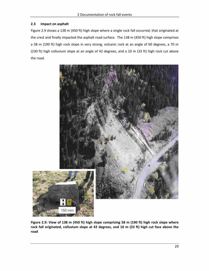
2 Documentation of rock fall events
29 30
2.3 Impact on asphalt
Figure 2.9 shows a 138 m (450 ft) high slope where a single rock fall occurred, that originated at
the crest and finally impacted the asphalt road surface. The 138 m (450 ft) high slope comprises
a 58 m (190 ft) high rock slope in very strong, volcanic rock at an angle of 60 degrees, a 70 m
(230 ft) high colluvium slope at an angle of 42 degrees, and a 10 m (33 ft) high rock cut above
the road.
Figure 2.9: View of 138 m (450 ft) high slope comprising 58 m (190 ft) high rock slope where rock fall originated, colluvium slope at 42 degrees, and 10 m (33 ft) high cut face above the road

2 Documentation of rock fall events
31
Table 2-5: Impact on asphalt
Impact point from source
(n)
Impact Coordinates Trajectory angle,
restitution from
horizontal, x axis (αf)
Slope angle
(above impact point)
s
Coefficients of restitution
Kinetic energy
lost during impact (J)
x co-ordinate
(m)
z co-ordinate, elevation
(m)
Normal coefficient
of restitution,
eN
Tangential coefficient
of restitution,
eT
Source 0.00 637.00
1 – rock 113.00 511.00 212.0 41.0 0.17 27.60 -570,123
2 – asphalt 124.00 501.00 118.0 0.0 0.38 0.24 -106,024
3 – 2nd impact 127.10 502.63
Figure 2.10 shows the final trajectories of the fall from the top of the 10 m (33 ft) high rock cut
to just after the impact on the road. These trajectories were precisely defined by a survey of the
site and the inset on Figure 2.10 shows the calculated velocity components at the asphalt impact
point. Although this is a single record of an impact with asphalt, the author has investigated
several similar events where comparable trajectories were generated for impacts on asphalt.
10 m
viN = -16.5 m · s-1
vf = 7.1 m ·s-1
vfT = 3.3 m · s-1
vfN = 6.3 m · s-1
eN = 0.38eT = 0.24
θf = 62˚
viT = 13.8 m ·s-1
θi = 50˚
vi = 21.5 m · s-1
-ω
Detail of velocity componentsat impact point on asphalt
viN = -16.5 m · s-1
vf = 7.1 m ·s-1
vfT = 3.3 m · s-1
vfN = 6.3 m · s-1
eN = 0.38eT = 0.24
θf = 62˚
viT = 13.8 m ·s-1
θi = 50˚
vi = 21.5 m · s-1
-ω-ω
Detail of velocity componentsat impact point on asphalt
α0 = 212°
α0 = 118°
1
2
3
Figure 2.10: Final trajectory of a rock falling from a height of 136 m (445 ft) and impacting a horizontal asphalt surface
The trajectory shown in Figure 2.10 is a relatively steep angle impact (i.e., θi = 50 degrees)
compared to the shallow angle impacts at Tornado Mountain and the Oregon test site, and for

2 Documentation of rock fall events
32
this condition the value of eN is 0.38. As discussed in Chapter 5, the value of eN for steep impacts
is low compared to shallow impacts. The value for eT for this relatively smooth impact surface is
0.24.
Analyses of these rock falls using the program RocFall 4.0 are given in Section 7.5.5.
Typical rock fall properties: cuboid block with axes lengths 0.84 m (2.8 ft), 0.58 m (1.9 ft) and
0.4 m (1.3 ft), mass of 500 kg or 1100 lb (unit weight of 26 kN · m-3 or 165 lbf · ft-3), and radius of
gyration of 0.295 m (1 ft).
2.4 Impact with concrete
Tests were conducted to find the normal restitution coefficient of concrete. The tests involved
dropping a boulder from a known height (hi) on to a horizontal concrete slab and measuring the
rebound height (hf). It was found that the normal coefficient of restitution eN for the concrete
under these impact conditions was 0.18 (eN = (vf/vi) = √(hf/hi) – see also Section 5.2.2, Figure 5.6
(Masuya et al., 2001).
2.5 Summary of case study results
This section summarizes the conditions at each of the documented case studies (Table 2-6) and
the calculated normal and tangential coefficients of restitution (Table 2-7).

2 Documentation of rock fall events
33
Table 2-6: Summary of rock properties
Site Mt. Stephen,
Canada
Kreuger Quarry, Oregon
Ehime, Japan
Tornado Mt., Canada
Highway (asphalt)
Geology
Strong, massive,
horizontally bedded
limestone containing
thin but widely
spaced shale beds
Hard durable basalt
Horizontally bedded
sandstone and
mudstone, with talus
Rock face in very strong,
massive limestone, talus and
colluvium on slope
Approx 60 m of rock
slope, 70 m of colluvium
(sand & gravel) and 8
m of rock cut
Slope angle (deg)
60 76 43 30 47
Dimension
ellipsoidal block with
axes lengths 0.4 m (1.3 ft), 0.4 m (1.3 ft)
and 0.2 m (0.7 ft)
cubic block with side
lengths 0.6 m (2 ft)
cubic concrete
block with side lengths
of 0.6 m (2 ft)
ellipsoidal block
(Boulder A) with axes
lengths 1.6 m (5.2 ft),
1.3 m (4.3 ft) and
1.3 m (4.3 ft)
cuboid block with axes lengths
0.84 m (2.8 ft), 0.58 m (1.9 ft) and
0.4 m (1.3 ft)
Radius (m) 0.2 0.3 0.3 0.8 0.36
Radius of gyration
0.13 m or 0.43 ft
0.245 m (0.80 ft)
0.245 m (0.80 ft)
0.46 m (1.5 ft)
0.295 m (1 ft)
Mass 44 kg (97 lb) 580 kg (1280
lb) 520 kg
(1,150 lb) 3750 kg (8300 lb)
500 kg or 1100 lb
Table 2.7 summarizes the calculated normal and tangential coefficients of restitution for the five
case studies, as well as the results of a rock dropped vertically on to a concrete surface. The
tabulated results show that eN has a range of values that are greater than 1 for shallow angle
impacts and as low as 0.24 for steep angle impacts, and 0.18 for the vertical drop test on
concrete; Chapter 5 discusses the relationship between the angle of impact θi and eN.
The results for eT have a narrower range from 0.25 and 0.27 for relatively smooth asphalt and
colluvium surfaces, to 0.49 and 0.73 for rock and talus surfaces. The eT results show a trend
between low values for smooth, soft surfaces to higher values for rough, hard surfaces that is
consistent with frictional properties of rock surfaces.
Chapter 4 (impact mechanics) and Chapter 5 (coefficients of restitution) discuss the theoretical
relationship between the values of eN and eT, and impact conditions. In addition, Section 4.7

2 Documentation of rock fall events
34
compares the final velocities and angles for the five case studies discussed in this chapter, with
the calculated final velocities and angles based on impact mechanics theory.
Table 2-7: Summary of coefficients of restitution calculated for rock fall case studies
Site no.
Rock fall site Slope
material Normal coefficient of
restitution, eN Tangential coefficient
of restitution, eT
1 Mt. Stephen,
Canada rock 0.75 0.68
2 Oregon ditch study (rock face impact)
rock 2.51 0.59
2 Oregon ditch study
(ditch impact) rock 0.24 0.55
3 Ehime, Japan
(rock slope, #3) rock 1.70 0.49
3 Ehime, Japan
(talus slope, #6) talus 0.22 0.73
3 Ehime, Japan
(talus slope, #7) talus 5.48 0.71
4 Tornado Mountain,
Canada colluvium 1.29 0.27
5 Highway asphalt 0.38 0.24
6 Drop test, Japan (see Figure 5.6)
concrete 0.18 -

3 Rock fall velocities and trajectories
35 35
3 Rock fall velocities and trajectories
Analysis of rock falls involves study of both trajectories and impacts. This chapter discusses
trajectories and how they depend on the translational and angular velocities of the falling
bodies. Also discussed are physical characteristics of rock fall sites such as run-out distance,
dispersion of falls in the run-out area and the influence of gullies on rock fall behavior.
Trajectories are defined by the distance between impact points and the height of the rock fall
path above the ground surface. In a few instances it is possible to measure these two
parameters in the field, as was the case with the two rock falls at Tornado Mountain discussed
in Section 2.2.2 where impacts with trees and the ground could be used to precisely define
trajectories. Figure 3.1 shows examples of well-defined impact points.
Figure 3.1: Examples of impact points visible in the field. a) Distance successive impact points on slope surface (Christchurch, New Zealand 2011 earthquake); b) impact point on tree showing trajectory height (Tornado Mountain, Canada)
3.1 Trajectory calculations
The trajectories that rock falls follow are exactly defined by Newtonian mechanics, assuming
that no air resistance occurs. This section defines the basic equations that govern trajectories,

3 Rock fall velocities and trajectories
36
and how these are applied to the analysis of rock falls to determine the location of impact
points, and the height and length of trajectories.
3.1.1 Trajectory equation
The trajectory portion of rock falls between impacts, that is, the flight path and changes in the
translational velocity, is governed by Newtonian mechanics and gravitational acceleration. The
calculations are based on acceleration in the vertical direction being equal to gravity (az = -g),
with no acceleration in the horizontal direction (ax = 0). Figure 3.2 shows a body moving with an
initial velocity V0 in direction α0 relative to a horizontal [x] and vertical [z] co-ordinate system.
Determination of the vertical and horizontal co-ordinates of the falling rock, and its velocity Vt,
at any time t during the trajectory, involves integration between the start of the trajectory at
time t = 0 and time t, of the following expressions for acceleration and velocity.
Vertical acceleration, az = -g; horizontal acceleration, ax = 0
Vertical velocity, t
ztz dtaV0
; horizontal velocity, t
xtx dtaV0
= -g · t + c = c´
At the start of the trajectory when t = 0, the velocity components are:
Vtz = v0z = c and Vtx = V0x = c’
Vtz = -g · t + V0z Vtx = V0x
Vertical location, t
z dtVtgz0
0 )( ; horizontal location, t
x dtVx0
0 )(
''2
10
2 ctVtgz z x =V0x·t + c’’’ (3.1)
When t = 0, z = 0, x = 0 and c’’ = c’’’ = 0
Therefore: tVtgz z 0
2
2
1 ; x = v0x·t or
xVxt
0
(3.2)
where V0z and V0x are respectively, the velocity components in the vertical and horizontal
directions at the start of the trajectory.
Equations (3.2) defines a parabolic curve, that gives the [x, z] co-ordinates of rock fall
trajectories, and other projectiles, as a function of time of flight, t.

3 Rock fall velocities and trajectories
37
The angle α0, measured counter-clockwise from the positive x axis, defines the direction of the
velocity vector V0 at time t = 0 (Figure 3.2) from which the following expressions can be
obtained:
x
z
V
V
0
00tan and 000 cosVV x (3.3)
Equations (3.2) and (3.3) can be combined to define the location of the body in terms of [x, z]
co-ordinates, the initial velocity v0 and angle α0 as shown in equation (3.4):
0
2
00
tancos2
x
V
xgz (3.4)
Figure 3.2: Definition of trajectory velocity components and directions
Equation (3.4) can be rearranged to show the relationship between the initial velocity V0 , of the
body, its angle relative to the x-axis α0, and the distance travelled by the body from the initial
point to the point defined by the co-ordinates [x, z]1:
5.0
00
0
)tan(2cos
g
zx
xV
(3.5)
1 Equation (3.5) can also be used for applications other than rock falls. For example, for water discharging from a pipe, the vertical and horizontal distances of the jet from the discharge point can be measured as well as the angle of the pipe. These values can be entered in equation (3.5) to find the discharge velocity, from which the flow rate can be calculated knowing the discharge area.

3 Rock fall velocities and trajectories
38
Worked example 3A – trajectory co-ordinates: if the initial velocity, V0 = 20 m · s-1 at an angle
α0 = 35 degrees, the vertical and horizontal components of the initial velocity are:
V0z = 20 sin 35 = 11.5 m · s-1; V0x = 20 cos 35 = 16.4 m · s-1
and the co-ordinates at time t = 2 seconds are given by equation (3.2):
z = -(0.5) · (9.81) · (2)2 + (11.5)· (2) = 3.38 m
If t = 4 seconds, z = -32.5 m, showing that, at this time when x = 65.6 m, the body has descended
below the x-axis and now has a negative z value.
3.1.2 Nomenclature – trajectories and impacts
The nomenclature used to define the velocities and angles of trajectories and impacts is shown
in Figure 3.3. For trajectories, the start of the trajectory is designated by the subscript “0” (time,
t = 0) and the end of the trajectory where the next impact starts is designated by the subscript
“i” (time, t = i).
With respect to the impact, the moment of impact at the end of the trajectory is designated by
the subscript “i” (e.g. Vi, θi), and the end of the impact and the start of the next trajectory by the
subscript “f” (e.g. Vf, θf). That is, Vf = V0 and θf = θ0, and the velocity at the end of the impact
equals the velocity at the start of the next trajectory. The final velocity and angle are also
termed the “restitution” parameters. Chapter 4, Impact Mechanics discusses methods of
calculating velocity components during impact.
3.1.3 Rock fall trajectories
The trajectory equations discussed in Section 3.1.1 can be applied directly to the analysis of rock
falls to determine parameters such as impact and restitution velocities, and trajectory lengths
and heights.
Figure 3.3 shows a typical rock fall configuration at the completion of an impact where a body is
just leaving the ground (impact point (n)) at a final (restitution) velocity Vf, equal to the velocity
at the start of the trajectory, V0. The orientation of this velocity vector can be defined by either
of two angles, α0 or θ0. The angle α0 is relative to the positive x-axis, measured either counter-
clockwise (positive) or clockwise (negative) and can have values between 0 and 360 degrees.
Angle α0 is used for the application of equations (3.1) to (3.5); in applying these equations,

3 Rock fall velocities and trajectories
39
values of α0 of +330 degrees or -30 degrees, for example, give identical results. That is, α0 = -30
degrees is equivalent to α0 = +330 degrees because sin (-30) = sin (330) = (-0.5).
The angle θ0, at the start of the trajectory, is used to define the orientation of the velocity vector
relative to the ground surface, and is a parameter that is more readily used in the analysis of
field data. If the slope angle is ψs, then the relationship between these three angles is given by:
θ0 = (ψs + α0) (3.6)
Equation (3.6) is applied for positive and negative values of α0.
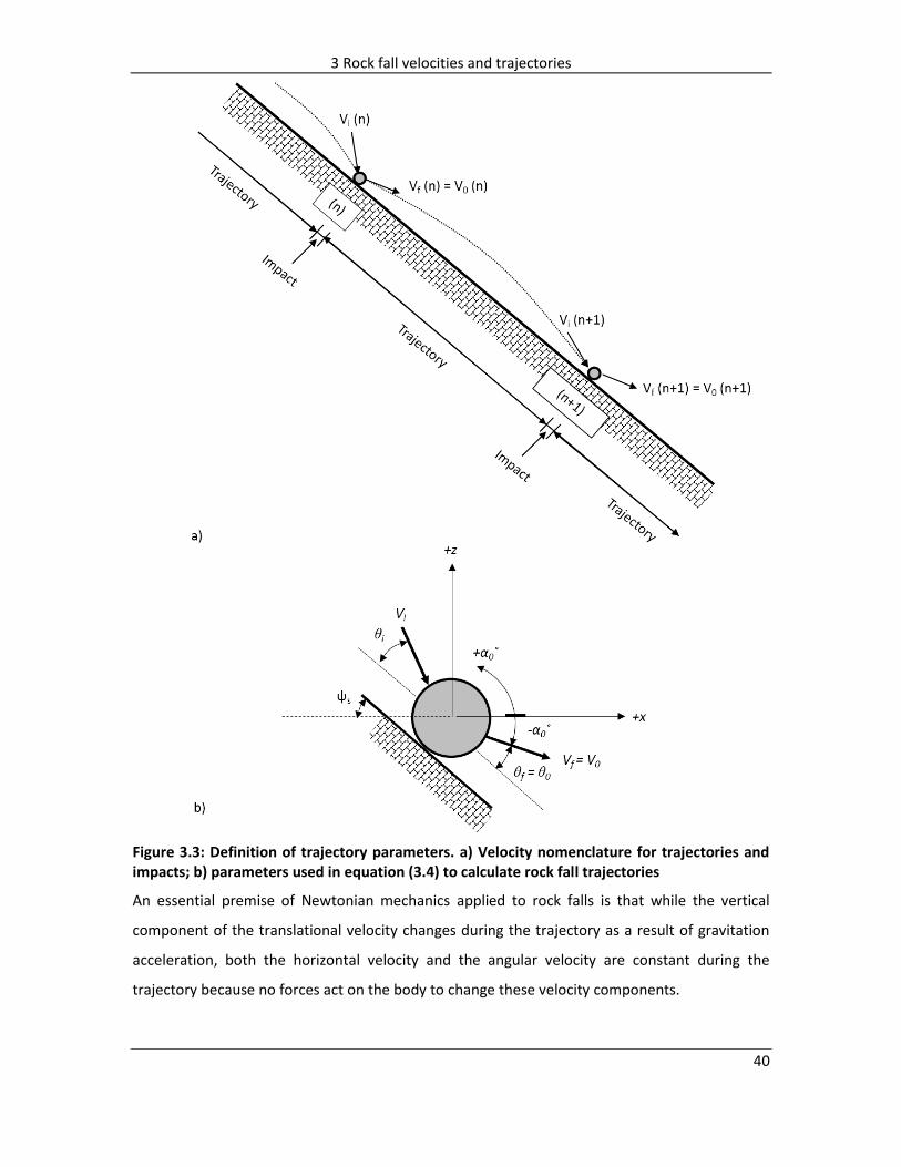
3 Rock fall velocities and trajectories
40
Figure 3.3: Definition of trajectory parameters. a) Velocity nomenclature for trajectories and impacts; b) parameters used in equation (3.4) to calculate rock fall trajectories
An essential premise of Newtonian mechanics applied to rock falls is that while the vertical
component of the translational velocity changes during the trajectory as a result of gravitation
acceleration, both the horizontal velocity and the angular velocity are constant during the
trajectory because no forces act on the body to change these velocity components.

3 Rock fall velocities and trajectories
41
The full trajectory of the rock fall, defined by the [x, z] co-ordinates, can be obtained from
equation (3.4) for specified values of V0, θ0 and ψs. Figure 3.4 shows successive locations of a
rock fall following a parabolic trajectory between impact points (n) and (n+1).
3.1.4 Trajectory height and length
The trajectory equations discussed in Section 3.1.1 above that define the rock fall path through
the air, can also be used to find the next impact point, the slope distance between impact
points, and height of the rock fall above the slope surface. These data are useful in designing
the location and height of fences and barriers on the slope.
Figure 3.4 shows the calculated trajectory between impact points (n) and (n+1) for the velocity
vector and slope angle parameters at point (n), where the velocity at the start of the trajectory
Vo is equal to the velocity at the completion of impact at point (n), or Vf(n). The co-ordinates of
impact point (n+1) can be found from the point of intersection between the equations for the
trajectory and slope. If the average slope between the impact points has gradient κ, then the
equation of the slope is:
z = κ · x (3.7)
and the point of intersection is found by equating equations (3.4) and (3.7) as follows:
tancos2
2
0
x
V
xgx
and
2
0 cos
1
)tan(2
Vg
ximpact (3.8)
Once the x co-ordinate of the impact point is known, it can be substituted in either equation
(3.4) or (3.7) to find the z co-ordinate.
The trajectory equation can also be used to find the vertical height h of the body above the
slope at any point, as well as the maximum height hmax, and the x co-ordinate of this height. The
height of the body above the slope is equal to the difference in z co-ordinates given by
equations (3.2) and (3.7).
h = (ztraj – zslope)

3 Rock fall velocities and trajectories
42
= (a · x2 + b · x) – (κ·x)
= (a · x2) + x(b-κ) (3.9a)
where
2
0 cos
1
2
V
ga and tanb (3.9b)
Equations (3.9a) and (3.9b) define the height of the body above the slope for any value of the
horizontal co-ordinate [x].
The maximum height of the body above the slope can be found by differentiation of equation
(3.9a), and equating the result to zero. The differential of equation (3.9a) is
)(2 bxadx
dh (3.10)
and the value of the x co-ordinate where the height is a maximum is:
a
bx
2
)( (3.11)
This value of x can then be substituted in equation (3.9a) to calculate the maximum trajectory
height, hmax (Figure 3.4).

3 Rock fall velocities and trajectories
43
Figure 3.4: Trajectory calculations showing rock fall path, impact points, impact velocities and trajectory height and length
Worked example 3B – trajectory calculations: a rock fall comprises a series of impacts with a
slope at a uniform angle ψs = 40 degrees (gradient, κ = -0.84). At impact point (n) with co-
ordinates [0, 0], the velocity at the start of the trajectory is V0(n) = 18 m · s-1 (Figure 3.4), and the
angle of the velocity vector at this point is θ0(n) = 20 degrees. The angle α0 defining the
orientation of the velocity vector can be found from equation (3.6) to be α0 = -20 degrees.
Based on these parameters, the co-ordinates of any point on the parabolic trajectory can be
found from equation (3.4):
z = -0.017x2 – 0.36x
The equation of the slope is (z = -0.84 x), so the co-ordinates of the next impact point (n+1) can
be found from equating these two expressions for z. The co-ordinates of impact point (n+1) are:
[x(n+1) = 28.2 m, z(n+1) = -23.8 m].
The slope length L between these two impact points is obtained from the difference Δ, of their
vertical (z) and horizontal (x) co-ordinates:

3 Rock fall velocities and trajectories
44
L = (Δx2 + Δz2)0.5
= 36.8 m
From equation (3.11), the maximum vertical height of the trajectory above the slope is 3.39 m,
which occurs at x co-ordinate 14.0 m.
It is also possible to calculate the impact velocity at impact point (n+1), Vi(n+1) as follows. The
horizontal and vertical components of the velocity at impact point (n) at the start of the
trajectory are respectively:
V0x(n) = V0(n) cos α = 16.9 m · s-1 and V0z(n) = V0(n) sin α = 6.2 m · s-1
During the trajectory to impact point (n+1), the vertical velocity component will increase due to
gravitational acceleration and the vertical velocity at point (n+1) is:
)(22
)(0)1( zgVV nzniz
= 22.4 m · s-1
The horizontal velocity component will not change during the trajectory so that the two
components of the impact velocity at impact point (n+1) are Vix(n+1) = 16.9 m · s-1 and Viz(n+1) =
22.4 m · s-1 . The resultant impact vector at point (n+1) has a velocity of Vi(n+1) = 28.1 m · s-1. The
angle θi(n+1) of the vector is given by:
916
4221
.
.tana)n(i 53 degrees
at an angle of αi(n+1) = 180 - 53 = 127 degrees.
3.1.5 Field trajectory heights
Section 3.1.4 above and Figure 3.4 show the calculated theoretical trajectory height measured
vertically from the slope surface for a parabolic rock fall trajectory. Information on actual
trajectory heights is available from the Ehime test site in Japan where the test blocks comprised
concrete spheres with a diameter of 0.54 m (1.8 ft), concrete cubes with a side length of 0.6 m
(2 ft) and blocks of rock with masses ranging from 120 kg to 2060 kg (260 lb to 4550 lb). The test
program consisted of 10 spheres, 10 cubes and 20 blocks of rock, with half of the tests carried
out on a treed slope and the second half after the trees had been removed (see Section 6.6
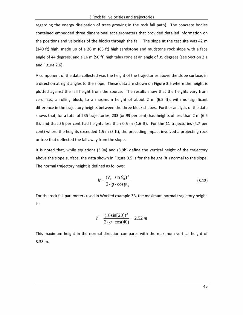
3 Rock fall velocities and trajectories
45
regarding the energy dissipation of trees growing in the rock fall path). The concrete bodies
contained embedded three dimensional accelerometers that provided detailed information on
the positions and velocities of the blocks through the fall. The slope at the test site was 42 m
(140 ft) high, made up of a 26 m (85 ft) high sandstone and mudstone rock slope with a face
angle of 44 degrees, and a 16 m (50 ft) high talus cone at an angle of 35 degrees (see Section 2.1
and Figure 2.6).
A component of the data collected was the height of the trajectories above the slope surface, in
a direction at right angles to the slope. These data are shown on Figure 3.5 where the height is
plotted against the fall height from the source. The results show that the heights vary from
zero, i.e., a rolling block, to a maximum height of about 2 m (6.5 ft), with no significant
difference in the trajectory heights between the three block shapes. Further analysis of the data
shows that, for a total of 235 trajectories, 233 (or 99 per cent) had heights of less than 2 m (6.5
ft), and that 56 per cent had heights less than 0.5 m (1.6 ft). For the 11 trajectories (4.7 per
cent) where the heights exceeded 1.5 m (5 ft), the preceding impact involved a projecting rock
or tree that deflected the fall away from the slope.
It is noted that, while equations (3.9a) and (3.9b) define the vertical height of the trajectory
above the slope surface, the data shown in Figure 3.5 is for the height (h´) normal to the slope.
The normal trajectory height is defined as follows:
sg
Vh
cos2
)sin('
2
00
(3.12)
For the rock fall parameters used in Worked example 3B, the maximum normal trajectory height
is:
mg
h 52.2)40cos(2
])20sin[18('
2
This maximum height in the normal direction compares with the maximum vertical height of
3.38 m.
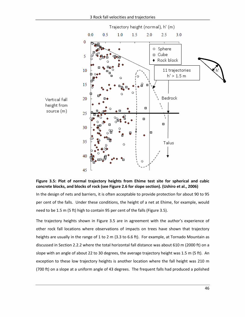
3 Rock fall velocities and trajectories
46
Figure 3.5: Plot of normal trajectory heights from Ehime test site for spherical and cubic concrete blocks, and blocks of rock (see Figure 2.6 for slope section). (Ushiro et al., 2006)
In the design of nets and barriers, it is often acceptable to provide protection for about 90 to 95
per cent of the falls. Under these conditions, the height of a net at Ehime, for example, would
need to be 1.5 m (5 ft) high to contain 95 per cent of the falls (Figure 3.5).
The trajectory heights shown in Figure 3.5 are in agreement with the author’s experience of
other rock fall locations where observations of impacts on trees have shown that trajectory
heights are usually in the range of 1 to 2 m (3.3 to 6.6 ft). For example, at Tornado Mountain as
discussed in Section 2.2.2 where the total horizontal fall distance was about 610 m (2000 ft) on a
slope with an angle of about 22 to 30 degrees, the average trajectory height was 1.5 m (5 ft). An
exception to these low trajectory heights is another location where the fall height was 210 m
(700 ft) on a slope at a uniform angle of 43 degrees. The frequent falls had produced a polished
3 Rock fall velocities and trajectories
47
rock surface on the well-defined rock fall path, and in the lower part of the slope, trajectory
heights of up to 4 m (13 ft) were observed.
3.2 Rock fall velocities
Section 3.1 above discussed trajectory paths with respect to their height and length, and the
equations that define these characteristics. This section discusses rock fall velocities, and the
conditions that influence velocity.
When a rock fall involves a series of impacts and trajectories, the velocity will increase if the
energy lost due to plastic deformation of the slope during impact is less than the energy gained
due to gravitational acceleration during the subsequent trajectory. Eventually, as the slope
angle flattens and/or the energy absorbing properties of the slope increase from bare rock to
soil, for example, the energy losses on impact will exceed the energy gains during the trajectory,
and the velocity will decrease.
3.2.1 Field velocity measurements
Typical velocities for the Ehime test site in Japan, as a function of the fall height, are shown in
Figure 3.6, in which the impact (Vi) and restitution (Vf) velocity components are shown
separately (see Figure 2.6 for slope section). The plot shows that impact velocities are greater
than restitution velocities, representing the loss of energy at the impacts; the variation in the
velocities is the result of the details of differing geometric conditions at the impact points.
Features of the plot in Figure 3.6, which are typical of rock falls, are that the velocities increase
in the early part of the fall over a height of about 15 m (50 ft) in this case, and then reach an
approximate terminal velocity of about 15 to 18 m · s-1 (50 to 60 ft · s-1). The plot also shows
that velocities in the rock and talus portions of the slope, with the velocities on the talus being
somewhat less than those on the rock. The velocities decrease at fall heights greater than 40 m
(130 ft) where the rocks roll past the base of the talus slope on to flatter ground and stop
moving.

3 Rock fall velocities and trajectories
48
Figure 3.6: Range of velocities for Ehime rock fall test site (see Figure 2.6 for slope section)
3.2.2 Effect of friction and slope angle on velocity
The main site characteristics that influence rock fall velocities, in addition to the fall height, are
the slope angle and the material(s) on the slope surface, with lower velocities for shallow slopes
and softer, more energy absorbing material compared to higher velocities for steep, hard rock
slopes. The relationship between velocity and height, incorporating the slope angle and the
characteristics of the slope material, is discussed below.
Referring to Figure 3.7a), a block of rock with mass m, is sliding on a slope dipping at ψs degrees
with the surficial material having an effective friction coefficient μ´. The motion of this block can
be studied using limit equilibrium methods that compare the relative magnitudes of the driving
and resisting forces (Wyllie and Mah, 2002). If the driving force is greater than the resisting
force, then the out-of-balance force (m · a), causes acceleration a, of the block according to the
following relationship:

3 Rock fall velocities and trajectories
49
)( forceresistingforcedrivingam
)cos'sin( ss gmgm
s
sga
tan
'1sin
Referring to Figure 3.7b), the velocity V, of the block sliding down the sloping plane over a
distance S is:
s
HaSaV
sin
222
and the rock fall velocity expressed in terms of the vertical fall height H is:
5.0
tan
'12
s
HgV
(3.13)
Figure 3.7: Velocity of rock fall on slope dipping at ψs: a) limit equilibrium forces acting on sliding block; b) relationship between free fall height, H and sliding distance, S
Equation (3.13) can also be expressed in the following manner:
5.02 Hg
V
(3.14)
where η is a parameter representing the slope characteristics:

3 Rock fall velocities and trajectories
50
5.0
tan
'1
s
(3.15)
or 21tan' s (3.16)
The parameter μ´ is an effective friction coefficient that incorporates both the material forming
the slope surface and the roughness of this surface. As the result of extensive field testing of
rock falls in Japan, values for the effective friction coefficient μ´ have been determined as shown
in Table 3.1 (Japan Road Association, 2000).
Table 3-1: Values of effective friction coefficient μ´ for characteristics of slope materials
Slope category
Characteristics of slope surface materials Design μ´ values*
Range of μ´ from
field tests
A Smooth, strong rock surfaces and uniform slope profile;
no tree cover. 0.05 0.0 to 0.1
B Smooth to rough, weak rock surfaces with medium to
high roughness slope profile; no tree cover. 0.15 0.11 to 0.2
C Smooth to rough, weak rock, soil, sand or talus with low
to medium roughness slope profile; no tree cover. 0.25 021 to 0.3
D Talus with angular boulders exposed at surface,
medium to high roughness slope profile; no tree cover or few trees.
0.35 ~0.31
* These values for μ´ tend to give upper bound velocity values.
Referring to Figure 3.6, the series of dashed curves show the relationship between values of η
and the measured rock fall velocities. When η = 1 and HgV 2 , the curve shows the free
fall velocity. For values of η less than 1, the velocity decreases as shown by the set of curves for
η values of 0.8 to 0.2.
Worked example 3C – fall velocities: the Ehime test site has two slope components: a 26 m high
rock slope at an average angle of 44 degrees, and a 16 m high talus slope at an angle of 35
degrees (see Sections 2.1 and 2.2, and Figure 2.6). From Table 3.1, the approximate friction
coefficients are 0.15 for the rock and 0.35 for the talus.
Figure 3.6 shows the measured velocities at the site, together with curves representing values
for the parameter η. On Figure 3.5, the maximum velocities correspond to values of η of ηrock =
0.9 and ηtalus = 0.7, equation (3.16) gives values for the friction coefficients as follows:

3 Rock fall velocities and trajectories
51
μ´rock = tan 44 (1 – 0.92) = 0.18 and for talus, μ´talus = tan 35 (1 – 0.72) = 0.36
Comparison of these calculated values for μ´ with the values shown on Table 3.1, shows that
equation (3.13) gives values for the maximum velocities if the friction angles given in Table 3.1
are applied.
In another example, at Tornado Mountain (see Section 2.2 and Figure 2.8) where the slope has
low roughness comprising gravel and soil, the impact velocities are in the range of 10 to
15 m · s-1 on the lower part of the slope where the slope angle is 22 degrees and the fall height
H, is about 250 m. The value for η is given by (equation (3.14):
39.0)2502(
5.125.0
g and μ’colluvium = tan 22 (1 – 0.392) = 0.34
This value for μ´colluvium is consistent with values for the friction coefficient given in Table 3.1 for
talus.
These back analyses for the relationship between velocity, slope angle and friction show that the
friction coefficients given on Table 3.1 can be used to estimate velocity values, although these
velocities may be at the high end of the actual velocity values.
The relationships in equations (3.12) to (3.14) and the effective friction coefficients shown in
Table 3.1 are used in Japan to estimate fall velocities and impact energies in the design of
protection structures. The application of these relationships to the Ehime and Tornado rock fall
sites illustrates that this is a useful method to estimate rock fall velocities when no field data are
available.
3.3 Variation of trajectories with restitution angle
This section discusses the variation of the angle at the start of the trajectory θ0, following an
impact, and its influence on the length and height of trajectories. This can be an important
factor in the design of protection structures that should be positioned at low trajectory and low
velocity locations on the slope.
3.3.1 Calculated trajectories for varying restitution angles (θ0)
Figure 3.8 shows two possible trajectories between a pair of impact points, (n) and (n+1) on the
slope dipping at angle ψs = 30 degrees, together with the initial velocities and angles at point (n).
At the start of the trajectory, the body leaves the slope with a restitution velocity V0, and at

3 Rock fall velocities and trajectories
52
angle θ0 relative to the slope surface. The [x, z] co-ordinates of the body at any point during the
trajectory can be calculated using equation (3.4). Figure 3.8 shows the successive positions of
the body for two possible trajectories defined by the initial angles θ0 = 15 degrees and θ0 = 45
degrees. In applying equation (3.4) to calculate the [x, z] co-ordinates of the trajectories, the α0
angles for the upper and lower trajectories are respectively α0 = +15 degrees and α0 = -15
degrees, where α0 is defined by equation (3.6) - (α0 = θ0 – ψs).
Also, equation (3.5) can be used to calculate the velocity required for the body to reach the
impact point (point (n+1)) with co-ordinates: [xi = 14] and [zi = -8]. For the low angle trajectory
(θ0 = 15 degrees), the required velocity is 15.5 m · s-1 (50.9 ft · s-1), while for the higher angle
trajectory (θ0 = 45 degrees), the required velocity is only 9.3 m · s-1 (30.5 ft · s-1). That is, as the
height of the trajectory increases, the velocity required for the body to reach a defined point
decreases.
Figure 3.8: Trajectories related to restitution angle, θ0: θ0 = 15 degrees and θ0 = 45 degrees
3.3.2 Field values of restitution angles (θ0)
Studies of the rock falls at Tornado Mountain and Ehime in Japan discussed in Chapter 2, have
been carried out to investigate the variation in restitution angles θ0 that occurs in the field
(Figure 3.9a) and b)).

3 Rock fall velocities and trajectories
53
For the two Tornado Mountain rock falls (see Section 2.2.2), the co-ordinates for a total of 114
impact points were measured in the field from which it was possible to determine the slope
length and inclination of each trajectory. However, it was only possible to determine the
trajectory path from equation (3.4) if information was also available on the magnitude of the
angle α0 defining the inclination of the initial velocity relative to the x-axis (Figure 3.2). This
information was provided at 21 locations along the trajectories where rock falls impacted trees
and it was possible to measure the height of the impact, and the distance of the tree from the
preceding impact point. These measurements provided three points on the parabolic path of
the rock fall from which the trajectory parameters, including the value of the angle α0, could be
precisely calculated.
From the 21 calculated values of α0 angles and the measured slope angle ψs between the two
impact points on the slope, values of the initial angle θ0 were calculated using equation (3.6). It
was found that the values of θ0 ranged from 6 to 63 degrees, a difference of 57 degrees, with an
average value of 33 degrees (Figure 3.9a)). That is, the impact process caused the restitution
angle to vary from a shallow angle in which the block barely left the slope surface, to larger
angles where the block follows a relatively high trajectory. Analysis of trajectories shows that
the height of the trajectory does not significantly influence the distance between impact points
because the restitution velocity decreases as the trajectory height increases, i.e., high angle
trajectories have velocities that are less than shallow angle trajectories.
A particular feature of the Tornado Mountain site is the uniform slope, at an angle of between
22 to 30 degrees, composed of gravel and soil with essentially no surface roughness or
irregularities. Therefore, variation in the restitution angle would be entirely the result of the
attitude of the rotating, irregular block as it impacted the slope.
Values of restitution angles were also measured at the Ehime test site (see Sections 2.1 and 2.2)
using data from the embedded accelerometers and high speed cameras (Figure 3.9b). The slope
materials comprised weak rock in the upper 25 m (80 ft) and talus in the lower part of the slope.
The values of θ0 ranged from about 5 to 55 degrees, with an average of 26 degrees, discounting
two outlying values between 65 and 70 degrees (Figure 3.9b). The histogram also shows the θ0
values for spherical and cubic concrete blocks, and blocks of rock. It may be expected that the
spherical blocks would show less variation than the more irregular cubes and blocks of rock, but
Figure 3.9b) shows that the distribution of θ0 values is similar for all three block shapes.

3 Rock fall velocities and trajectories
54
The two plots in Figure 3.9a) and b) are similar with respect to both range and form of the
distributions, despite the significantly different site characteristics. This range of θ0 values
accounts for the variation of trajectories that are usually observed in the field, even where
conditions are similar for each impact. An additional factor influencing variations in the values
of the angle θ0 is the angular velocity of the block as discussed in Section 3.4 below.

3 Rock fall velocities and trajectories
55
a)
b)
θ0
vf
Figure 3.9: Ranges of values for restitution angle, θ0. a) Tornado Mountain tree impacts (21 points); b) Ehime test site trajectory measurements for spherical, cubic concrete blocks and blocks of rock (Ushiro et al., 2006)
3 Rock fall velocities and trajectories
56
3.4 Angular velocity
Measurement of angular velocity of rock falls in the field requires the use of high speed
cameras, or embedded accelerometers in concrete blocks as used at the Ehime test site in
Japan.
3.4.1 Field measurements of angular velocity
For the rock falls at the 42 m (140 ft) high Ehime test site in Japan, the rotational velocity was
accurately measured throughout the fall. The tests were conducted on spherical concrete blocks
(diameter 0.54 m (1.8 ft)) and cubic concrete blocks (side length 0.6 m (2 ft)), as well as 20
irregularly shaped blocks of rock with masses ranging from 120 to 2060 kg (260 lb to 4550 lb)
(see Section 2.2).
Figure 3.10 is a plot relating the measured angular velocity ω, to the fall height, H for the Ehime
test site. The data shows that the range of angular velocities was 6 to 33 rad · s-1. For the first
10 m (30 ft) approximately of the fall height, ω increases with each impact, and thereafter the
blocks rotate at a terminal velocity that ranges between about 12 and 30 rad · s-1. That is, at
each successive impact, the angular velocity may increase or decrease depending on the
attitude of the blocks as they impact the slope.
Further analysis of the data on Figure 3.10 shows the relationship between the dimensions and
shapes of the blocks and the angular velocity. The range of angular velocities shown in Figure
3.10 is similar for all three block shapes, with the spherical and cubic concrete blocks reaching
slightly higher angular velocities of about 32 rad · s-1 than that for the irregular blocks of rock at
27 rad · s-1.
The angular velocity measurements have also been analyzed to show the relationships between
the translational and angular velocities at the start of the trajectory v0 and ω0, respectively of
the blocks and their dimensions r. The theoretical relationship between these three parameters
is as follows:
r
V00
or 0
0
Vr (3.17)
3 Rock fall velocities and trajectories
57
For the three types of blocks used at the Ehime test site, the following values were obtained for
values of the radius r, as defined by equation (3.17).
Spheres with radius, r = 0.27 m,
0
0
V 0.2 to 0.54 m
Cubes with side length 0.6 m and semi-diagonal length, r = 0.42 m,
0
0
V 0.25 to 0.7 m
Blocks of rock with an average radius, r = 0.65 m,
0
0
V 0.3 to 1.0 m
For all three types of block, the theoretical relationship defined by equation (3.17) is reasonably
consistent with the field values. That is, the actual radius of the rotating body lies within the
range of field values for the ratio (V0/ω0). Also, the tests showed that the range of field values
for the ratio (V0/ω0) is wider for irregularly shaped blocks of rock than for the more uniform
concrete spheres and cubes.
These results indicate that the relationship given by equation (3.17) can be used to estimate
values for the angular velocity of blocks with known dimensions and velocities.
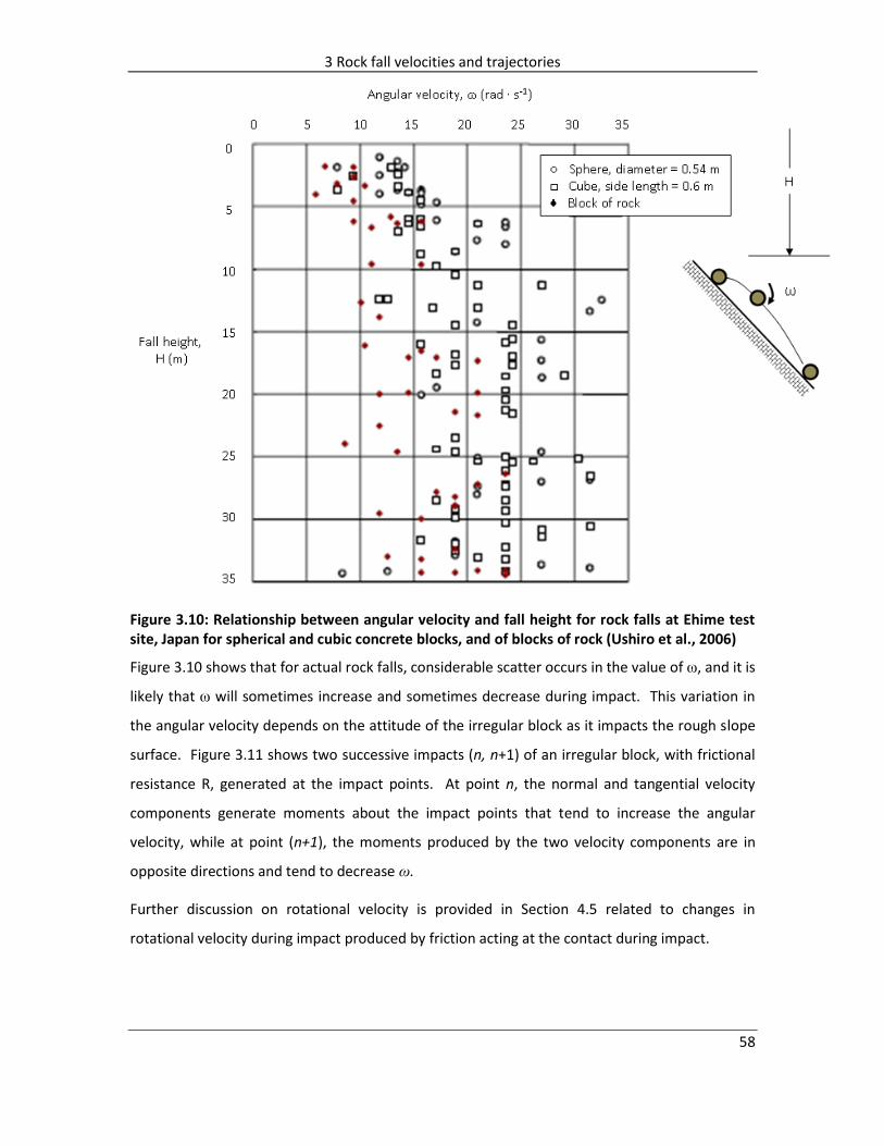
3 Rock fall velocities and trajectories
58
Figure 3.10: Relationship between angular velocity and fall height for rock falls at Ehime test site, Japan for spherical and cubic concrete blocks, and of blocks of rock (Ushiro et al., 2006)
Figure 3.10 shows that for actual rock falls, considerable scatter occurs in the value of ω, and it is
likely that ω will sometimes increase and sometimes decrease during impact. This variation in
the angular velocity depends on the attitude of the irregular block as it impacts the rough slope
surface. Figure 3.11 shows two successive impacts (n, n+1) of an irregular block, with frictional
resistance R, generated at the impact points. At point n, the normal and tangential velocity
components generate moments about the impact points that tend to increase the angular
velocity, while at point (n+1), the moments produced by the two velocity components are in
opposite directions and tend to decrease ω.
Further discussion on rotational velocity is provided in Section 4.5 related to changes in
rotational velocity during impact produced by friction acting at the contact during impact.

3 Rock fall velocities and trajectories
59
Figure 3.11: Effect of attitude of block during impact on angular velocity
3.4.2 Relationship between trajectories and angular velocity
For a perfectly elastic impact of a smooth, non-rotating block, the impact and restitution
velocities and angles will be identical. However, for actual rock falls where the block is rotating
with frictional resistance being developed at the impact point and plastic compression of the
slope materials occurring, the restitution parameters will change during impact.
Impact mechanics theory discussed in Chapter 4 shows that the effect of clockwise rotation as
shown on Figure 3.11, for a frictional impact is to flatten the trajectory, i.e. reduce the value of
θ0. Also, the higher the clockwise angular velocity, the smaller the value of θ0 with a flatter
trajectory. Furthermore, as the trajectory becomes flatter (closer to the slope surface), the
velocity increases as shown in Figure 3.8 where two trajectory paths are compared.
Impact mechanics also shows that the effect of counter clockwise rotation is to produce higher,
slower trajectories.
3.5 Field observations of rock fall trajectories
This section briefly describes some of the characteristics of rock fall trajectories in the field.

3 Rock fall velocities and trajectories
60
3.5.1 Rock falls down gullies
Rock falls on steep slopes are similar to water flow in that falls will tend to concentrate in gullies.
That is, minor gullies in the upper part of the slope act as a “water shed” in which falls over a
wide area on the upper slope combine into a single gully at the base of the slope. For example,
at one active rock fall site, falls were originating from a maximum height of about 250 m (820 ft)
over a slope length of about 120 m (400 ft), but they were almost all contained by a 12 m (40 ft)
long fence in a gully at the base of the slope. This shows that careful examination of the rock fall
geometry can result in substantial savings in construction of protection measures.
Another effect of rock falls concentrating in gullies, is that the fall path is not a straight line
down the maximum gradient line. Figure 3.12 shows a slope about 500 m (1,640 ft) high on
which rock falls are entirely concentrated into three, sinuously-shaped gullies in which the rock
fall paths are significantly longer and flatter than the slope cross-section. This shows that rock
falls can be much more accurately modeled in three dimensions than in two dimensions. That
is, cross sections of the slope shown in Figure 3.12 would be irregular where the section crossed
the gullies, and modeling of this slope would probably show significant trajectory heights where
falls impacted the sides of the gullies. In contrast, a section down a gully would be an essentially
uniform slope in which trajectory heights would probably not exceed 2 m (6.6 ft).
Figure 3.12 also shows how all rock falls over a length of several hundred meters along crest can
be contained by just three fences located in the base of the gullies, each about 20 m (65 ft) long.

3 Rock fall velocities and trajectories
61
Figure 3.12: Mountain slope with three sinuous gullies in which all rock falls are concentrated
3.5.2 Run-out distance
The maximum distance that a rock fall will travel from the source zone can be an important
parameter in the location and/or protection of facilities in the run-out area. Figure 1.1 shows a
typical rock fall site made up of four areas – the rock face where the fall originates, a colluvium
slope, a talus slope where most of the rock falls accumulate, and a run-out zone, or rock fall
“shadow area”, between the base of the talus cone and the maximum travel distance. The
maximum travel distance is defined by a line drawn at a dip angle of 27.5 degrees from the base
of the rock face to the intersection with the ground surface (Hungr and Evans, 1988).
Depending on the level of risk acceptance for the facilities, the run-out area could be
designated an exclusion zone in which no continuously occupied structure such as a house,
could be located. Alternatively, it may be acceptable to locate such facilities as a lightly used

3 Rock fall velocities and trajectories
62
road or a golf course within the run-out zone, perhaps with some protection such as a ditch
along the up-slope edge.
Section 8.5.5 discusses the application of decision analysis to rationally evaluate the cost benefit
of alternate rock fall protection measures based on the probability of rock falls occurring, the
consequence of such falls, and the cost of constructing protection measures.
3.5.3 Dispersion in run-out area
Where a talus cone has developed at the base of a rock fall area, over time falls will disperse
uniformly over the talus to build up the cone equally over its full area. This is a progressive
process whereby the accumulation of rock falls on one area of the cone will then divert
subsequent rock falls to a lower area that is built up in turn.
At the Ehime test site discussed in Chapter 2, it was found that the falls dispersed over an area
subtended by an angle of 60 degrees, with about 93 per cent of the falls within a 30 degree
angle. At other test sites in Japan, the angle defining the width of the dispersal area varied from
45 to 70 degrees (Ushiro and Hideki, 2001). At Tornado Mountain, the horizontal distance
between the two rock falls was 87m (285 ft) after falling 740 m (2450 ft), or a dispersion angle of
7 degrees.
This information can be used to determine the length of rock fall fence that may be required to
contain falls.
4 Impact mechanics
63 63
4 Impact mechanics
The theory of impact mechanics is used in a wide variety of fields (Goldsmith, 1960; Stronge,
2000) and builds on earlier work carried out by Sir Isaac Newton (Newton, 1687) and others
such as Poisson and Hertz in the 19th century. The theories generally apply to the impact
between two bodies, made of different materials, that are both translating and rotating,
have unequal masses and are moving in three dimensional space. For rock falls, the impact
conditions are somewhat simplified because one of the bodies (the slope) is stationary and
has infinite mass. However, the roughness of the slope and irregularity of the rock falls
introduces complexities in the modeling that can be accounted for by probabilistic analyses.
Furthermore, the theory needs to account for the condition that the two bodies are not be of
the same material.
This chapter summarizes the application of impact mechanics theory to rock falls, and how
the theory can be applied to the actual rock fall events documented in Chapter 2. Chapters 5
and 6 cover respectively coefficients of restitution and energy losses, and show how the field
results can be used to calibrate impact mechanics theory and modeling programs.
The theory for impact mechanics described in this thesis is based primarily on the work of W.
J. Stronge (2000).
4.1 Principles of rigid body impact
The theory of impact mechanics can be applied to rock falls in order to understand the
impact process, and to develop algorithms for modeling rock falls. This work involves the
application of rigid body impact and kinetics to rock fall behavior as described below.
4.1.1 Rigid body impact
The particular physical conditions that are applicable to rock falls are low velocity (i.e., less
than about 40 m · s-1 (130 ft · s-1)), and impact of initially nonconforming hard, rigid bodies
that result in minor deformations but high stresses generated over the small area of the
impact, and to a very shallow depth. During impact, the shapes of the two surfaces are
briefly conformable. These contact conditions, in which no inter-penetration or adhesion of
the two bodies occurs, are referred to as low compliance impacts.

4 Impact mechanics
64
The highly stressed contact area of the rock fall and the slope can be considered as a short,
stiff spring, or an infinitesimally small, deformable particle (Figure 4.1). The spring or particle
is compressed during the compression phase of impact, and then releases energy to force
the rock fall away from the slope after the time of maximum compression and during the
restitution phase of impact.
The duration of the impact is very short, possibly a few tenths of a second, which has a
number of implications for modeling rock falls. First, changes to the position of the rock fall
are negligible during impact, and second, gravitational forces can be ignored because they
are very low compared to the high induced forces at the impact point.
Based on these assumed conditions of impact, the change in velocity of the rock fall during
impact can be resolved as a function of the normal component of impulse, where the normal
impulse is equal to the integral of the normal contact force over the time of the impact.
Since the impact involves only compression, and not extension of the spring or particle, the
normal component of impulse is a monotonously increasing function of time after impact.
Thus, variations in velocity during impact are resolved by choosing as an independent
variable the normal component of impulse, pN, rather than time. This principle gives velocity
changes during impact that are a continuous, smooth function of impulse (Stronge, 2000).
Throughout this thesis, impacts are modeled in terms of the relationship between changes in
normal and tangential relative (between the periphery of the body and the slope) velocity
components, vN and vT, and the normal component of impulse, pN.
Figure 4.1: Forces generated at contact point during normal impact

4 Impact mechanics
65
4.1.2 Kinetics of rigid bodies
Kinetics is a means of examining the change in velocity of the body when forces act on the
body during impact.
A rock fall is a rigid body as defined in Section 4.1.1 above, and can be considered as a point
mass, of infinitesimal size. If the body has mass m and is moving with velocity V (at the
center of gravity), then the momentum of the body is (m · V). If a resultant force F acts on
the body, this causes a change in momentum according to Newton’s second law of motion.
Second Law: the momentum (m · v), of a body has a rate of change with respect to
time that is proportional to, and in the direction of, any resultant force F(t) acting on
the body.
Assuming that the mass of the body is constant during impact, then the change in velocity is
a continuous function of the impulse, p. The forces F, -F acting on the rock fall and the slope
that prevent interpenetration of the two bodies are related by Newton’s third law of motion:
Third law: two interacting bodies have forces of action and reaction that are equal in
magnitude, opposite in direction and collinear, i.e., F = - F.
The application of the second and third laws to rock falls is shown in the following sections.
4.2 Forces and impulses generated during collinear impact
Calculation of the forces and impacts during rock fall impacts applies Newton’s second and third
laws discussed in Section 4.1.2 above.
The impact process for a non-rotating, rigid body moving with relative velocity vN and impacting
a stationary surface at right angles can be simulated with an infinitesimal, deformable particle at
the contact point between the two bodies (Figure 4.1). The particle acts as a short, stiff spring
that, during impact, generates equal and opposite reaction forces F, -F at the point of impact
that are parallel to the velocity direction.
The reaction forces change the momentum of the body, and for a constant mass during impact,
the velocity is changed. The change in momentum generated by the impact produces a finite
impulse p that continuously changes the velocity during the impact time. During impact of a
body with mass m, a change in normal velocity occurs from viN at impact (time t = i) to vN at time

4 Impact mechanics
66
t. The normal component of impulse pN, generated by the normal component of the contact
force F(t) is given by the relationship:
dtFvvmdp iNNN (4.1a)
where dt
dvmF
dtdt
dvmdpN
m
dpdv N
N (4.1b)
and t
iNiNN pdtFvvm )( (4.1c)
The relative normal velocity vN at any time t during the impact can be obtained by integration,
for the limit that at the moment of impact t(i), the normal velocity is given by:
t
itNN dp
mv
)(
1 (4.2)
m
pvv N
iNN where viN < 0 (4.3)
The impacting normal velocity is negative because, as shown in Figure 4.1, the positive normal
axis is in the direction away from the point of impact.
Equation (4.3) shows that the normal component of the relative velocity is a linear function of
the normal impulse. This relationship between v and p is the basis for determining changes in
impulse during impact, and finding the terminal impulse pf, at the termination of impact (t = f)
when the body separates from the slope.
Equation (4.3) can also be used to find the impulse values at maximum compression (pcN). At
the point of maximum compression, the normal velocity is momentarily equal to zero and the
corresponding normal impulse has a value pcN given by equation (4.3)
m
pv cN
iN 0
and

4 Impact mechanics
67
iNcN vmp (4.4)
At the end of the impact (t = f), the final normal velocity is vfN and the final normal impulse (pfN)
can also be found from equation (4.3),
)( iffN vmvmp (4.5)
4.3 Energy changes during impact
The impact process results in compression δ of the deformable particle during the compression
phase (Figure 4.1), followed by expansion during the restitution phase. The changes in the
normal contact force F during impact are illustrated in Figure 4.2a) where the force (Fc) and
deformation (δc) are at a maximum at the end of the compression phase, followed by partial
recovery (δf), for inelastic impact, at the completion of the recovery phase. The recovery of
kinetic energy is the process that drives the bodies apart in the final phase of the impact after
maximum compression.
Figure 4.2b) shows the changes in the normal contact force as a function of time. The area
under the [t – F] curve up to time tc is the impulse pc generated during the compression phase
and represents the kinetic energy of relative motion converted into internal energy of
deformation. The area between times tc and tf is the change in impulse (pf – pc) and represents
the energy recovered during the restitution phase. The changes in velocity during impact can be
quantified in terms of the normal coefficient of restitution, eN that is the ratio of the final normal
velocity vfN to the impact normal velocity, viN.
On Figure 4.2b), for an elastic impact the two areas are identical - eN = 1, while for a perfectly
plastic impact no energy is recovered - eN = 0.
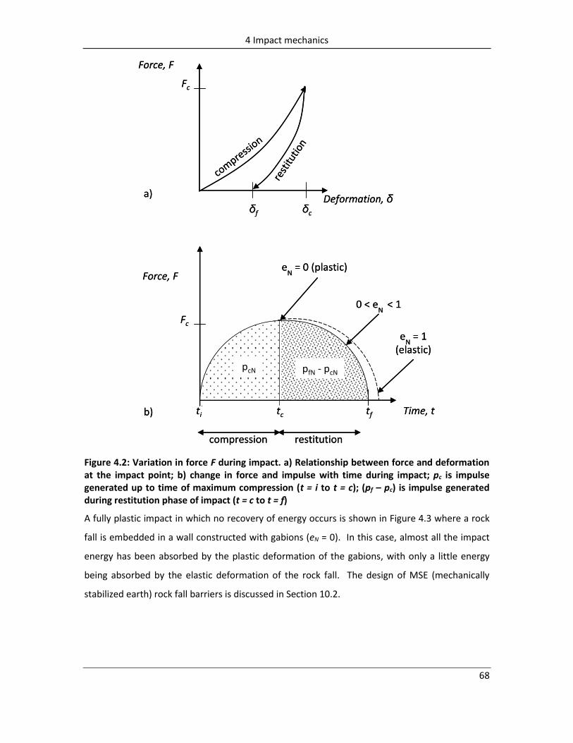
4 Impact mechanics
68
Force, F
Deformation, δ
compre
ssion
rest
itutio
n
a)
compression restitution
Fc
δcδf
Time, t
Fc
tc tf
eN
= 1 (elastic)
eN
= 0 (plastic)
0 < eN
< 1
b)
pcN pfN - pcN
Force, F
ti
Force, F
Deformation, δ
compre
ssion
rest
itutio
n
a)
compression restitution
Fc
δcδf
Time, t
Fc
tc tf
eN
= 1 (elastic)
eN
= 0 (plastic)
0 < eN
< 1
b)
pcN pfN - pcN
Force, F
ti
Figure 4.2: Variation in force F during impact. a) Relationship between force and deformation at the impact point; b) change in force and impulse with time during impact; pc is impulse generated up to time of maximum compression (t = i to t = c); (pf – pc) is impulse generated during restitution phase of impact (t = c to t = f)
A fully plastic impact in which no recovery of energy occurs is shown in Figure 4.3 where a rock
fall is embedded in a wall constructed with gabions (eN = 0). In this case, almost all the impact
energy has been absorbed by the plastic deformation of the gabions, with only a little energy
being absorbed by the elastic deformation of the rock fall. The design of MSE (mechanically
stabilized earth) rock fall barriers is discussed in Section 10.2.

4 Impact mechanics
69
Figure 4.3: Example of plastic impact where a rock fall is embedded in a gabion wall
4.4 Coefficient of restitution
The principle of separating the compression and restitution phases of impact can be
demonstrated on a normal impulse [(pN) – relative velocity (v)] plot as shown in Figure 4.4. On
this plot, the normal velocity changes during impact, starting with a negative value (-viN) at the
point of impact, increasing to zero at the point of maximum compression pc, and finally reaching
a positive value (vfN) at the point of separation. Also, the tangential velocity vT decreases
continuously during impact from viT at the point of impact, to vfT at the point of separation, as
the result of frictional resistance on the contact surface. The role of friction on impact behavior
is discussed in Section 4.5.

4 Impact mechanics
70
+N
vi
-viN
vf
vfT
vfN
viT
Velocity, v
compression restitution
viN
pcN pfN
Normal impulse, pN
viT
vfT
vfN
+T
EcN
EfN -EcN
Figure 4.4: Relationship between normal impulse pN and changes in tangential and normal velocities vT, vN, and energy during impact; EcN is the kinetic energy absorbed during the compression phase of impact (t = c); (EfN – EcN) is the strain energy recovered during the restitution phase (t = c to t = f)
The [pN – v] plot on Figure 4.4 shows the changes in both the normal (vN) and tangential (vT)
velocities, and the magnitude of the internal energy of deformation generated during impact.
These changes in velocity and energy can be quantified in terms of the coefficient of restitution2,
e that has normal and tangential components as follows:
iN
fN
Nv
ve (4.6)
and
iT
fT
Tv
ve (4.7)
The parameter eN, which is related to compression/hystersis at the contact point, is used to
determine the normal velocity and energy changes that occur during impact as discussed in this
chapter. The parameter eT, which quantifies the changes in tangential velocity during impact, is
2 In this treatment of impact mechanics as it applies specifically to rock falls, the term coefficient of restitution is used to quantify the changes in both velocity and energy, and it encompasses the terms kinetic, kinematic and energetic coefficients of restitution that apply in certain impact conditions (Stronge, 2000).

4 Impact mechanics
71
a function of the friction acting on the contact surface and the effect of friction on the angular
velocity of the body.
Examples of actual changes in normal and tangential velocities during impact and the
corresponding values of eN and eT are discussed in the documentation of rock fall events
discussed in Chapter 2, and are listed in Table 2.1.
With respect to the energy of deformation, the triangular area EcN in Figure 4.4 represents the
kinetic energy of normal motion that is absorbed in compressing the deformable region, while
triangular area (EfN – EcN) represents the elastic strain energy recovered during restitution. The
expression for the energy change during compression is:
dpm
pvdpvE
cN cNp pN
iNNcN
0 0
m
ppv cN
cNiN2
2
since pcN = - m · viN (equation (4.4))
2
2
1iNcN vmE (4.8)
and the energy change during restitution is:
fN
cN
fN
cN
p
p
p
p
NNiN
NiNcNfN
m
ppvdp
m
pvEE
2)(
2
2
2 12
1
cN
fN
iNp
pvm (4.9)
where viN < 0.
Derivation of equations (4.8) and (4.9) is shown in Appendix B. Equations (4.8) and (4.9) are also
derived in Chapter 6 that discusses energy losses during impact.
The expressions in equations (4.8) and (4.9) for the partially irreversible changes in kinetic
energy of normal motion that occur during impact can be used to define the normal coefficient
of restitution, eN as follows:

4 Impact mechanics
72
)(
)()(2
cNN
cNNfNN
NpE
pEpEe
(4.10)
This definition of the coefficient of restitution where the impulse is an independent variable,
separates the energy loss due to compression and hysteresis of the contact forces from that due
to friction and slip between the colliding bodies. As shown in Figure 4.2, the value for eN can
range from eN = 1 for a perfectly elastic material where no loss of energy occurs during impact,
to eN = 0 for a perfectly plastic material where no separation occurs during impact and no
recovery of the initial kinetic energy occurs.
Also, the relationships shown in equations (4.8), (4.9) and (4.10) can be combined, for normal
impact, to find the following expression for the normal coefficient of restitution in terms of the
normal impulses at maximum compression (pcN) and at the completion of the impact (pfN):
2
2 1
cN
fN
Np
pe (4.11)
Substitution of the expressions for pcN and pfN in equations (4.4) and (4.5) into equation (4.11),
yields the following expression relating impulse to the coefficient of restitution:
)1()1( NcNNiNfN epevmp (4.12)
and for the normal coefficient of restitution,
iN
fN
Nv
ve (4.6)
cN
cNfN
Np
ppe
)( (4.13)
As shown in Figure 4.4 and expressed in equations (4.6) and (4.13), the normal coefficient of
restitution is the ratio of final normal velocity to the impact normal velocity, and is also the
square root of the negative ratio of the energy recovered during the restitution phase of the
impact to the energy lost during the compression phase (equation (4.10)).
For rough bodies where slip occurs at the contact point, but the direction of slip is constant, the
two expressions for the coefficient of restitution in equations (4.6) and (4.13) are equivalent.

4 Impact mechanics
73
4.5 For frictional angular velocity changes during impact, for rough surface
For oblique impact of a rock fall with a slope, the impulse acting at the contact point gives an
impulsive moment about the centre of mass of the rock fall (Figure 4.5). This impulsive moment
changes the angular and translational velocities during the period of contact.
Changes in the rotational and translational velocities during impact can be attributed to friction
at the rock-slope contact. According to Coulomb’s definition of friction, the coefficient of
friction μ, is the ratio of the tangential to normal forces acting at the contact point.
Furthermore, the ratio of the tangential to normal forces is a constant such that the friction
coefficient is also a constant that is independent of the slip velocity and the normal force.
It is noted that in rock mechanics, it is usually assumed that the coefficient of friction decreases
with increasing normal stress due to breakdown of the asperities on the rough rock surfaces
during shear movement. However, for rock fall impacts that are of short duration and have
limited shearing distance, the friction coefficient is considered to be independent of the normal
force.
When a translating and rotating body impacts a stationary slope, slip will initially occur between
the two bodies and frictional forces will be generated at the contact point. In accordance with
the usual concept of friction relating normal and tangential impulses, slip of the body on the
slope is assumed to occur at the value of limiting friction, requiring that
pT = |μ · pN| (4.14a)
while slip stops and the body rolls during impact when
(pT ≤ μ · pN) (4.14b)
This transition from slip to rolling is illustrated on Figure 4.5. The behavior of a rotating body
during impact can be demonstrated on the [normal impulse (pN) – relative velocity (v)] plot on
Figure 4.5. For a spherical body with radius r and rotating at angular velocity -ω, the velocity at
the periphery of the body (-r · ω) is parallel, but opposite in direction, to the translational
tangential velocity vT. If the magnitudes of |r · ω| and vT are unequal, then slip will occur
between the moving body and the stationary ground, with the slip velocity vS, being given by:
vS = vT + r · ω (4.15)

4 Impact mechanics
74
The direction of rotation is negative if the peripheral velocity (r · ω) is in the opposite direction
to the positive tangential axis. For rock falls, the angular velocity is usually negative because the
tangential translational velocity acting down slope and the friction force (μ · pN) acting upslope
interact to spin the rock clockwise as shown in Figure 4.5.
The slip velocity depends on the both the magnitude and direction of the angular velocity
relative to the tangential velocity as defined by equation (4.15) and shown on Figure 4.5. If the
angular velocity is negative, then the slip velocity is less than the initial tangential velocity
(Figure 4.5a)), while if the angular velocity is positive, the slip velocity is greater than the initial
tangential velocity (Figure 4.5b)).
Depending on the details of the impact process, the values of (r · ω) and vT may equalize during
impact, in which case slip will cease at impulse psN and from this point the body will roll with no
change in angular velocity. In other conditions related to the attitude of the irregular body
impacting the slope, slip may continue throughout the impact.
The [pN – v] plot in Figure 4.5 also shows that the tangential velocity decreases during the slip
phase of the impact from viT to vfT. This reduction in tangential velocity can be attributed to the
friction force acting at the contact between the impacting body and the slope, and to the
irregularities of the slope at the impact point. Equations developed in Section 4.6 show the
slope of the tangential velocity line.
The [pN – v] plots in Figure 4.5 show the angular velocity increasing during the slip phase (ωs >
ωi). However, for irregularly shaped, rotating blocks impacting the slope at a variety of
attitudes, the velocity components may combine under some conditions to reduce the velocity
during impact, rather than increasing with each impact (see also Figure 3.11). At the Ehime test
site described in Sections 2.1.3 and 2.2.1, the rotational velocities of about 100 test blocks on
the 42 m (140 ft) high slope varied between 6 and 33 rad · s-1. The measured values of ω at
Ehime are plotted against the fall height on Figure 3.10 and show that while ω does generally
increase during the fall, low values for ω occur in the lower part of the fall showing that some
impact conditions can result in the rotational velocity decreasing during impact.
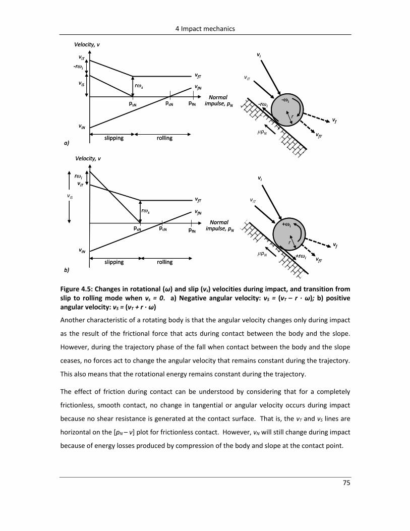
4 Impact mechanics
75
vi
vf
vfT
viT
-ωi-rωi
μpN
r
slipping rolling
viN
pcN pfN
viT
vfT
vfNviS
psN
rωs
-rωi
Normal impulse, pN
Velocity, v
vi
vf
vfT
viT
+ωi
+rωiμpN
r
slipping rolling
viN
pcN pfN
viT
vfT
vfN
psN
rωs
rωi
Normal impulse, pN
Velocity, v
viS
a)
b)
vi
vf
vfT
viT
-ωi-rωi
μpN
r
slipping rolling
viN
pcN pfN
viT
vfT
vfNviS
psN
rωs
-rωi
Normal impulse, pN
Velocity, v
vi
vf
vfT
viT
+ωi
+rωiμpN
r
slipping rolling
viN
pcN pfN
viT
vfT
vfN
psN
rωs
rωi
Normal impulse, pN
Velocity, v
viS
a)
b)
Figure 4.5: Changes in rotational (ω) and slip (vs) velocities during impact, and transition from slip to rolling mode when vs = 0. a) Negative angular velocity: vS = (vT – r · ω); b) positive angular velocity: vS = (vT + r · ω)
Another characteristic of a rotating body is that the angular velocity changes only during impact
as the result of the frictional force that acts during contact between the body and the slope.
However, during the trajectory phase of the fall when contact between the body and the slope
ceases, no forces act to change the angular velocity that remains constant during the trajectory.
This also means that the rotational energy remains constant during the trajectory.
The effect of friction during contact can be understood by considering that for a completely
frictionless, smooth contact, no change in tangential or angular velocity occurs during impact
because no shear resistance is generated at the contact surface. That is, the vT and vS lines are
horizontal on the [pN – v] plot for frictionless contact. However, vN will still change during impact
because of energy losses produced by compression of the body and slope at the contact point.

4 Impact mechanics
76
4.6 Impact behaviour for rough, rotating body
When a rock fall impacts a slope, the parameters defining the impact conditions are the
translational and rotational velocities at the moment of impact (t = i), and the impact angle
relative to the slope (θi). In addition, the characteristics of the slope are defined by the normal
coefficient of restitution, and the friction coefficient. In order to model rock fall behavior, it is
necessary to calculate the final translational and rotational velocities (t = f), and the angle at
which the body leaves the slope. These three final parameters can then be used to calculate the
subsequent trajectory of the body. This section describes how impact mechanics can be used to
derive the equations defining changes in velocity components and angles during impact. The
impact mechanics model discussed in this section is based on the work of Stronge (2000) and
Goldsmith (1960) on collision between solid bodies, with modifications to suit the particular
conditions of rock falls.
The theory of impact mechanics can be used to model impact between two irregularly shaped,
rough, rotating bodies moving in three dimensional space; for rock falls, the model can be
simplified by making one of the bodies (the slope) stationary and of infinite mass. For the
purpose of developing equations to model impact in this thesis, further simplifications will be
made that friction is developed at the impact point, and the body is moving in two-dimensional
space (plane motion) (Figure 4.6). The size and shape of the body are defined by the radius (r)
and the radius of gyration (k).
The equations of motion are referenced to coordinate axes set up at the impact point in
directions normal N and tangential T to the slope surface. The positive normal axis is away from
the slope and the positive tangential axis is down-slope such that the impact normal velocity is
negative and the tangential velocity is positive. In addition, the angular velocity is negative
when it is in the –T direction at the contact point. Subscript “i” refers to conditions at impact
(time, t = i), and subscript “f” refers to restitution conditions at the end of impact (time, t = f).
The radius of the spherical body is r.

4 Impact mechanics
77
vf
vi
-viN
vfT
vfN
viT
+N
θi
θf
-ωi
μpN
r-rωi
+T
vf
vi
-viN
vfT
vfN
viT
+N
θi
θf
-ωi
μpN
r-rωi
+T
Figure 4.6: Impact of rough, rotating sphere on a slope in plane motion
4.6.1 Impulse calculations
The impact of the rock fall with the slope in plane motion produces normal and tangential
impulses pN and pT respectively at the contact point that alter the normal and tangential
velocity components of the rock during impact. The velocity changes are governed by the
magnitude of the normal coefficient of restitution eN and the limiting value of the coefficient of
friction μ. Values of the coefficient of restitution have been determined by documenting actual
rock fall events as described in Chapter 2, and for the coefficient of friction from both laboratory
tests and rock fall events.
Figure 4.6 shows a body with mass m, radius r and radius of gyration k impacting the slope at a
shallow angle. Following the nomenclature defining impact velocities shown in previous
sections of this chapter, at any time during the impact, the linear impulse-momentum equation
(4.1c) provides the following relationship for the normal impulse pN related to the change in the
normal component of the velocity:
NiNN pvvm )( (4.1c)
And the equivalent tangential impulse equation pT :
TiTT pvvm )( (4.16)

4 Impact mechanics
78
where viT and viN are respectively the initial tangential and normal translational velocity
components at impact (time, t = i).
With respect to the rotation of the block with angular velocity ω at time t, initial angular velocity
ωi and moment of inertia I, the angular impulse-momentum equation is:
t
i dtrFIdI0
)()( (4.17)
and
rpkm Ti )(2 (4.18)
where I = m · k2 , and k is the radius of gyration of the body.
The volumes and radii of gyration of bodies that may simulate rock falls are listed in Table 4-1.

4 Impact mechanics
79
Table 4-1: Volume and radius of gyration of common rock fall body shapes
Body shape Volume, Ω Axial radius of gyration, k
Cube: side length L 3L 6
L – axis normal to face, or along diagonal
Sphere: radius r 3
3
4r r
5.0
5
2
Cylinder: length L, radius r Lr 2
5.022
12
3
Lr– axis through mid-height
(“tumbling” motion)
Ellipsoid: axes 2a, 2b, 2c cba 3
4
5.022
5
)(
ba– rotation about axis c
4.6.2 Final velocities for rock fall impacts
For a rotating rock fall impacting a slope at an oblique angle, the rock will have both
translational v, and angular ω, velocities, with the translational velocity expressed as normal and
tangential components relative to the slope surface (Figure 4.6). At the contact point, equal and
opposite forces, F, -F are developed that oppose interpenetration of the rock into the slope and
give differentials of impulse dp in the normal and tangential directions that are related by:
dtFdp N (4.1a)
Newton’s second law (see Section 4.1.2), gives equations of motion for translation of the centre
of the rock fall mass in the normal N, and tangential T, planes:
m
dpdv N
N
and
m
dpdv T
T
and for planar rotation of the rock fall:
Ndpkm
rd
2 (4.19)
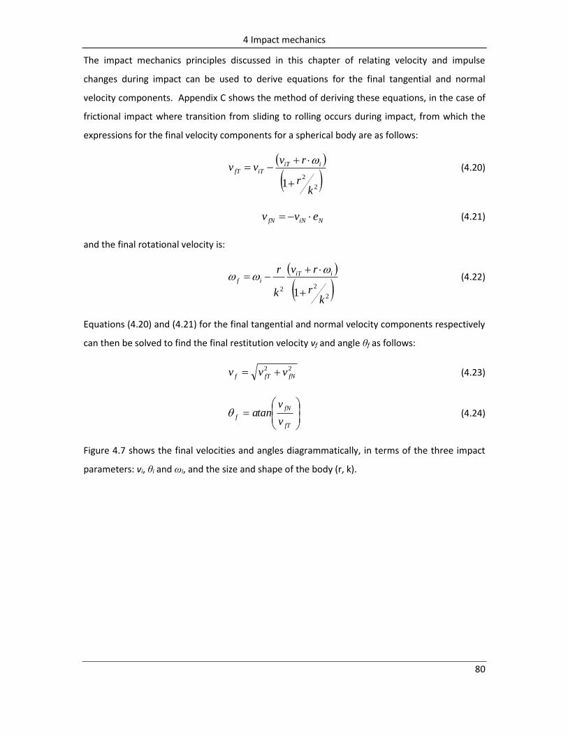
4 Impact mechanics
80
The impact mechanics principles discussed in this chapter of relating velocity and impulse
changes during impact can be used to derive equations for the final tangential and normal
velocity components. Appendix C shows the method of deriving these equations, in the case of
frictional impact where transition from sliding to rolling occurs during impact, from which the
expressions for the final velocity components for a spherical body are as follows:
2
2
1k
r
rvvv iiT
iTfT
(4.20)
NiNfN evv (4.21)
and the final rotational velocity is:
2
22 1k
r
rv
k
r iiTif
(4.22)
Equations (4.20) and (4.21) for the final tangential and normal velocity components respectively
can then be solved to find the final restitution velocity vf and angle θf as follows:
22
fNfTf vvv (4.23)
fT
fN
fv
vtana (4.24)
Figure 4.7 shows the final velocities and angles diagrammatically, in terms of the three impact
parameters: vi, θi and ωi, and the size and shape of the body (r, k).

4 Impact mechanics
81
vi
vf = ( vfT2 + vfN
2 )1/2
vfT
+N
+T
θi
θf
-ωi
viN = - vi sinθiviT = vi cosθi
vfN = - eN · viN
Equation (4.24)
= atan (vfN/vfT)
ωf = Equation (4.22)
vi
vf = ( vfT2 + vfN
2 )1/2
vfT
+N
+T
θi
θf
-ωi
viN = - vi sinθiviT = vi cosθi
vfN = - eN · viN
Equation (4.24)
= atan (vfN/vfT)
ωf = Equation (4.22)
Figure 4.7: Diagram of impact showing equations defining impact and restitution velocity vectors
It is of interest that in equations (4.20) to (4.24) defining the final velocities and restitution
angle, the only physical property of the slope/rock fall that is incorporated is the normal
coefficient of restitution. The friction coefficient, which relates tangential and normal impulses
during slip (Equation (4.14a)), is used to calculate the reduction in tangential velocity during
impact as shown in Appendix C, Section C.2. Also, Chapter 6 shows the calculation of energy
losses for rotating bodies incorporating the coefficient of friction.
When slip halts and the block rolls, no additional change in tangential velocity occurs because
sliding friction does not operate in this phase of the impact process. Furthermore, while the size
(radius, r) and shape (radius of gyration, k) of the body influences the final velocity and angle
calculations, these values are independent of the mass because the forces generated at the
impact point are much larger than gravity so body forces can be neglected (see Section 4.1). The
equations presented in this chapter demonstrate the basic behavior of a rough, rotating sphere
impacting a stationary slope surface, for a two-dimensional (planar) condition. If necessary, the
equations can be modified to analyze other block shapes such as ellipsoids or slabs. While the
equations are a simplification of actual rock fall behavior, they provide a useful framework for
understanding the various factors that influence rock fall behavior, and can be used to examine
actual rock falls and assist in the design of protection measures. Section 4.7 compares actual
velocities documented in Chapter 2 with velocities calculated from the theoretical equations.

4 Impact mechanics
82
4.6.3 Example of impact mechanics calculation
Correct application of the equations in this chapter requires careful attention to the signs
(negative and positive) of the velocities and angles according to the system of axes as shown in
Figure 4.6. The following worked example illustrates a sample calculation.
Worked example 4A – impact final velocities: for a 1.5 m diameter spherical rock fall, the
impact translational and rotational velocities (vi and ωi), and impact angle θi relative to the
slope, are shown in Figure 4.8. The tangential and normal components of the impact velocity
are calculated as follows:
19.19cos smvv iiiT ; 13.9sin smvv iiiN
The radius of gyration k of the sphere is r √(2/5) = 0.47 m.
The coefficient of restitution eN is determined from the relationship between θi and eN as
discussed in Chapter 5 (Section 5.2, equation (5.4)) where it is demonstrated that:
03.15.19
iNe
= 0.71
vi = 22 m s-1
viN = -9.3 m s-1
vf = 18.7 m s-1
vfT = 17.5 m s-1
vfN = 6.6 m s-1viT = 19.9 m s-1
θi = 25˚
θf = 20.7˚
ωi = -15 rad s-1
ωf = -23.3 rad s-1
-ω
vi = 22 m s-1
viN = -9.3 m s-1
vf = 18.7 m s-1
vfT = 17.5 m s-1
vfN = 6.6 m s-1viT = 19.9 m s-1
θi = 25˚
θf = 20.7˚
ωi = -15 rad s-1
ωf = -23.3 rad s-1
-ω
Figure 4.8: Example of rock fall impact showing values calculated final (restitution) velocity and angle
Application of equations (4.20) to (4.24) gives the values for the final translational and angular
velocity components, and the restitution as shown on Figure 4.8. These results show that during

4 Impact mechanics
83
impact the normal velocity component changes from -9.3 m · s-1 towards the slope to +6.6m · s-1
away from the slope, while the tangential velocity component reduces from 19.9 to 17.5 m · s-1,
and the angular velocity increases, in the negative direction, from -15 to -23.3 rad · s-1. The
overall effect of the impact is to reduce the velocity of the rock by 3.3 m · s-1, or 15 per cent. The
final angle, θf = 20.7 degrees.
The effect of rotation on the impact process is illustrated by letting ωi = 0, for which the new
values for the calculated final velocities are: vfT = 14.2 m · s-1, ωf = -19 rad · s-1 and θf = 24.8
degrees. That is, the effect of a rotational velocity of -15 rad · s-1, compared to the body not
rotating at impact, is to increase vfT from 14.2 to 17.5 m s-1, and produce a flatter trajectory as θf
changes from 24.8 to 20.7 degrees.
4.6.4 Effect of angular velocity on trajectories
Worked example 4A and Figure 4.8 show the influence of the angular velocity on the restitution
velocity and angle. That is, an increasing negative angular velocity produces a flatter, greater
velocity trajectory. The impact mechanics equations can also be used to find the effect of
positive rotational velocity on trajectories as follows.
Equation (4.20) shows the relationship between the impact rotational velocity ωi and the
restitution tangential velocity vfT. Also, equation (4.21) relates the restitution normal velocity vfN
to the normal coefficient of restitution eN, and equations (4.23) and (4.24) can then be used to
find the restitution velocity vf and angle θf.
The influence of the impact angular velocity ωi on the restitution velocity and angle is shown in
Figure 4.9. In these three models, the impact velocity is vi = 22 m s-1 at angle θi = 25 degrees.
Impacts have been studied for three angular velocities: Model a) - ωi = -15 rad · s-1; Model b) - ωi
= -25 rad · s-1; Model c) - ωi = +15 rad · s-1. As shown on Figure 4.5, the angular velocity is
negative if its direction at the contact point is in the opposite direction to the positive tangential
axis, i.e., clockwise in this model.
The calculation of the final velocities and angles for the three conditions on Figure 4.9 confirms
that the effect of an increasing negative angular velocity is to increase the final velocity and
produce a flatter trajectory. That is, for conditions a) and b), the final velocity increases from
18.7 m · s-1 to 20.7 m · s-1, while the final angle decreases from 20.6 degrees to 18.6 degrees.

4 Impact mechanics
84
In model 4.9c), the body is rotating in a counter-clockwise (positive) direction, and the
restitution velocity now decreases to 12.9 m · s-1 at a larger angle of θf = 27.1 degrees.
In rock falls, rotation is almost always in the negative direction because the frictional resistance
at the contact between the slope surface and the moving body sets up a moment acting
clockwise. The calculations show that the negative angular velocity flattens the trajectory which
is consistent with the low trajectory heights shown on Figure 3.5. Furthermore, the distributions
of θf values plotted in Figures 3.9 a) and b) show that the majority of θf values are less than
about 30 degrees, with few high angle trajectories; that is, θf values greater than 60 degrees are
rare. An exception to this condition is for very shallow angle impacts (θi <15°) where high angle
final trajectories can occur (see Section 5.2).
Figure 4.9: Influence of impact angular velocity, ωi on restitution velocity, vf and angle, θf. a) ωi = -15 rad · s-1; b) ωi = -25 rad · s-1; c) ωi = +15 rad · s-1
Calculation of ωf using equation (4.22) shows that for a sphere, ωf will increase with every
impact. In fact, field studies show that the angular velocity may increase or decrease on impact,
depending on the attitude of the non-spherical block relative to the slope at the point of impact.
Measured values of ωf shown on Figure 3.10 illustrate the variation in ωf values, and that ωf may
increase or decrease during impact after the initial 5 to 10 m of fall height (see Section 3.4.1).

4 Impact mechanics
85
The trajectories of rock falls are important in the selection of appropriate heights for protection
structures such as fences and barriers. Both field data and impact mechanics theory show that
low trajectories are more common than high trajectories and this may be taken into account in
fence design.
4.7 Calculated vs. actual restitution velocities
Chapter 2 describes five rock fall events where the impact and restitution velocities and angles
were carefully documented; vectors of these velocities for a typical impact at each sites are
shown on the insets in Figures 2.2 to 2.10. Information is also available on the shape,
dimensions, radius and radius of gyration of a typical block at each site.
These actual restitution velocities can be compared with velocities calculated using equations
(4.20) to (4.24) in Section 4.6.2 based on impact mechanics theory. In applying these equations,
values are required for the initial angular velocity ωi, and the normal coefficient of restitution eN,
at the impact points. Values for these two parameters were obtained from the following
relationships:
r
vii (3.17)
where vi is the impact velocity and r is the radius of the body.
and
03.15.19
iNe (5.4)
where θi is the impact angle.
Figure 4.10 is a plot comparing the two sets of restitution velocities. The plot shows that the
calculated velocities are in all cases greater than the actual velocities by values ranging from 20
to 50 per cent. Sensitivity analyses of these calculations shows that the calculated and actual
values are closer when the angular velocity is reduced and the normal coefficient of restitution
is increased. However, reasonable changes to these parameters are not sufficient to make the
calculated velocities equal to the actual values.

4 Impact mechanics
86
Figure 4.10: Plot comparing restitution velocities – actual (Chapter 2) and calculated (equations (4.20) to (4.24)) values

5 Coefficient of restitution
87 87
5 Coefficient of restitution
The results of the field studies in Chapter 2 and the discussion of impact mechanics in Chapter 4
illustrate how rock fall behavior can be defined by values for the normal and tangential
coefficients of restitution (eN and eT) that are applicable to the particular site conditions. The
coefficients of restitution quantify velocity changes during impact and help in understanding
how conditions at the impact points influence rock fall behavior. Figure 5.1 shows three impacts
and two trajectories and clearly illustrates the reduced velocity and height of the second
trajectory due to the loss of energy at the first impact, i.e., eN < 1. Figure 5.1 shows typical
behavior of a rubber ball – rock falls will always have lower trajectories than these because of
the relatively low eN of rock.
Changes in the velocity components during impact and the corresponding coefficients of
restitution are also illustrated in Figure 5.2 on the [normal impulse, pN – relative velocity, v]
diagram. The normal coefficient of restitution defines the change in normal velocity during
impact and is related to the impact angle as discussed in this chapter, and the inelastic
compression of the slope materials. The tangential coefficient of restitution defines the
reduction in tangential velocity during impact and is related to the friction force generated
between the slope and the body. This chapter discusses how these coefficients are correlated
with impact conditions and are not purely material properties.
Figure 5.1: Impacts between successive trajectories showing typical inelastic behavior and loss of energy during impact where second trajectory (on right) is lower than first trajectory; rock falls will always have lower trajectories than those shown (Micheal Maggs, Wikimedia Commons)

5 Coefficient of restitution
88
This chapter summarizes the results of the eN and eT values obtained from the five field studies
described in Chapter 2, encompassing four different slope materials and 57 impacts. A sixth
location is a laboratory test where blocks of rock were dropped on to a concrete floor and the
rebound heights were measured to give values for eN.
vi
-viN
vf
vfT
vfN
viT
Velocity, v
compression restitution
viN
pcN pfN
Normal impulse, pN
viT
vfT
vfN
+N
+T
vi
-viN
vf
vfT
vfN
viT
Velocity, v
compression restitution
viN
pcN pfN
Normal impulse, pN
viT
vfT
vfN
+N
+T
Figure 5.2: Normal impulse-velocity plot showing relationships between changes in normal (N) and tangential (T) velocity components and coefficients of restitution – eN = (vfN/viN) and eT = (vfT/viT)
5.1 Newton’s coefficient of restitution
The concept of the coefficient of restitution, which in this case was the normal coefficient, was
first developed by Isaac Newton (1686) who suspended spheres of the same material on
pendulums and measured how high they rebounded after impact (Figure 5.3); the
measurements incorporated corrections for velocity losses due to air friction. Values for the
coefficient of restitution found by Newton included 0.56 for steel and 0.94 for glass. One of the
purposes of the experiments was to prove the Third law of motion – every action has an equal
and opposite reaction.
It was assumed at the time of Newton’s experiments that the coefficients of restitution were
material properties. However, it is now understood for impact between rough, rotating bodies
of different materials, such as rock falls, reductions in velocity depend not only on the material
forming the body, but also on the impact conditions such as mass and shape of the impacting
body, and the impact angle and velocity.

5 Coefficient of restitution
89
Figure 5.3: Isaac Newton's measurement of normal coefficient of restitution using impact of spheres suspended on pendulums
5.2 Normal coefficient of restitution
Equation (4.6) and the [pN – v] diagram shown on Figure 5.2 define the normal coefficient of
restitution as the ratio of the final to impact normal velocities:
i
f
iN
fN
Nh
h
v
ve (4.6)
where vfN (t = f) and viN (t = i) are the final (restitution) and impact velocities respectively, and eN
is negative because viN, acting in the negative direction of the normal axis, has a negative value.
Equation (4.6) indicates that the value of the normal coefficient can be determined by dropping
blocks of rock from height (hi) on to different surfaces and measuring the height of the rebound
(hf) in a similar manner to the procedure used by Newton. However, this is not applicable to
rock falls where the irregular, rotating blocks are impacting rough slope surfaces at oblique
angles. In fact, for rock falls, it is difficult to measure the value of eN in the laboratory because of
the complexity of the impact process. Field measurement of coefficients of restitution involves
carefully documenting impacts and trajectories, by locating impact points or using a high speed
camera, and then calculating the normal and tangential components of the impact and
restitution velocities.3
3 Because rock fall impacts differ significantly from Newtonian-type impacts (Figure 5.3), the ratio of final to impact normal velocities for rock falls (eN) may be termed the “apparent” coefficient of restitution. In this thesis, eN always refers to rock fall impacts where eN is not a material property, and can have a value greater than 1.

5 Coefficient of restitution
90
A further complication with the velocity measurements is that considerable scatter occurs in the
values as the result of the wide variation in the impact conditions of the rotating, irregular
blocks impacting the rough slope surface. This variation can best be handled using probabilistic
methods in which the design values of velocity, coefficient of restitution and rock fall mass are
expressed as probability distributions rather than discrete values. This result in turn means that
the design of protection structures can be based on probabilistic methods in which the structure
is designed to withstand, for example, impact of 90 per cent or 95 per cent of likely rock fall
energies rather than the largest event that may ever occur. Where these large events rarely
occur, the cost of providing protection against all rock falls would have to be balanced against
the likely consequence of the fall.
5.2.1 Theoretical relationship between impact angle and normal coefficient of restitution
The [normal impulse, pN – relative velocity, v] diagram in Figure 5.4a) illustrates the influence of
impact conditions on the normal coefficient of restitution eN, keeping in mind the discussion in
Section 5.1 that eN is not a material property, but depends on the impact characteristics. The
two dashed lines on Figure 5.4a) represent changes in the normal velocity during impact for two
identical, non-spherical eccentric impacts with respect to mass and impact translational velocity.
The approximate relationship between the normal impulse pN and the normal velocity vN is
assumed to be linear with gradient equal to (1/m).
m
pvv N
iNN (4.3)
On Figure 5.4a), the only difference between the two lines is the impact angles θi, θi´. The lines
show the change in normal velocity during impact from a negative value acting towards the
slope at the point of impact (t = i), to zero at the point of maximum compression (t = c), to a
positive velocity acting away from the slope at the end of the impact (t = f).
The upper dashed line on Figure 5.4a) represents a shallow angle impact close to the slope
surface, while the lower dashed line represents a steeper angle impact (θ'i < θi). For the shallow
impact, the normal velocity component is small relative to the normal component for the steep

5 Coefficient of restitution
91
impact (v´iN < viN). However, the slope of the [pN – v] line is the same for both impacts because
the mass is unchanged.
Examination of the final and initial normal velocities for the two impact conditions on Figure
5.4a) shows that e'N > eN , and that e'N > 1.0 for the shallow angle impact. A normal coefficient of
restitution that is greater than 1 does not mean that energy is created during the impact
process; e´N > 1 because the geometry of the impact results in the final normal velocity
component being greater than the impact vertical velocity component.
With respect to energy changes during impact, the final velocity will always be less than the
impact velocity (v'f < v'i and vf < vi ) resulting in a net loss of energy during impact (Giacomini, A.
et al., 2010; Buzzi, O. et al., 2012; Asteriou, H. et al., 2012; Spadari, M. et al., 2012). Energy
changes during impact are discussed in more detail in Chapter 6.
Figure 5.4a) also shows that the value of the normal impulse at maximum compression is also
influenced by the impact angle (pc > p'c). That is, a shallow impact results in a “softer” impact
than a steeper impact. For steep angle impacts, the body will cause more compression of the
slope material, compared to shallow angle impacts, resulting in less rebound and a smaller value
of vfN.
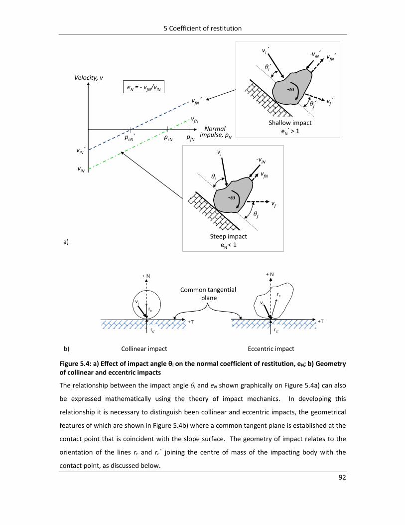
5 Coefficient of restitution
92
vi ´
vf´
θi´
θf´
-viN´ vfN´
-ω
Shallow impacteN´ > 1
vi
vf
θi
θf
-viN
vfN
-ω
Steep impacteN < 1
viN´
pcN pfN
vfN ´
vfN
viN
pcN´
Velocity, v
Normal impulse, pN
eN = - vfN/viN
a)
b) Collinear impact Eccentric impact
-ω
rc
rc’
+ N
vi
+T
rc
rc’
+ N
+T
vi+
+
Common tangentialplane
Figure 5.4: a) Effect of impact angle θi on the normal coefficient of restitution, eN; b) Geometry of collinear and eccentric impacts
The relationship between the impact angle θi and eN shown graphically on Figure 5.4a) can also
be expressed mathematically using the theory of impact mechanics. In developing this
relationship it is necessary to distinguish been collinear and eccentric impacts, the geometrical
features of which are shown in Figure 5.4b) where a common tangent plane is established at the
contact point that is coincident with the slope surface. The geometry of impact relates to the
orientation of the lines rc and rc´ joining the centre of mass of the impacting body with the
contact point, as discussed below.

5 Coefficient of restitution
93
Collinear impact – collinear impact occurs where the line between the centre of mass of the
impacting body lies on the normal to the common tangent plane; this will occur for a spherical
body. For these conditions, the equations of motion for normal and tangential directions can be
decoupled such that spin and friction do not contribute to the normal component of the final
velocity. That is, the normal coefficient of restitution is equal to the ratio of the final to impact
normal velocity components and will be less than 1.0.
Appendix C shows, for collinear impacts, the derivation of equations for the final translational
and angular velocities and the restitution angle relative to the slope for conditions where slip
stops during impact. These equations can be rearranged to find a mathematical relationship
between the final and impact angles, θf and θi as follows.
The restitution (final, t = f) angle θf is related to the final normal and tangential velocities as
shown in equation (4.24):
fT
fN
fv
vtan (4.24)
For a rough, rotating sphere, the final tangential (vfT) and normal velocities (vfN) are given by
equations (4.20) and (4.21) that can be combined with equation (4.24) as follows:
221
tan
krv
rvv
ev
iN
iiTiT
NiNf
(5.1)
Since the impact angle θi is related to the impact velocity components as follows
iT
iNi
v
vtan
equations (5.1) and (4.24) can be rearranged to show the relationship between θf and θi :
ii
i
Nif
cosv
r
kr
etantan
11
11
22
(5.2)
For an impacting sphere where k2 = r2 · (2/5) and (1+r2/k2)-1 = 0.29, equation (5.2) simplifies to:

5 Coefficient of restitution
94
ii
i
Nif
cosv
r..
etantan
2901710
(5.3)
Equations (5.1) to (5.3) are applicable to collinear impact conditions.
Eccentric impact – for actual rock falls where the body is non-spherical and rough, and impact
occurs at an oblique angle, eccentric impact conditions apply as defined in Figure 5.4b). For
these conditions, the line rc from the centre of mass of the impacting body does not lie on the
on the normal to the common tangent plane, and the equations of motion each involve both
normal and tangential forces, such that the effects of friction and normal forces are not
separable.
For both collinear and eccentric impact, Goldsmith (1960) provides a graphical solution for
finding the final impulses, velocities and angles. These plots show how the normal and
tangential impulses vary throughout the duration of impact, and are related to the impact angle
and the friction at the contact point. Also, the normal impulse decreases as the impact angle
becomes shallower, which is consistent with the impact model shown in Figure 5.4a).
Figure 5.5: Relationship between impact angle θi and normal coefficient of restitution eN with best fit (power) curve for average values of θi and eN each material type

5 Coefficient of restitution
95
5.2.2 Field data showing relationship between impact angle and normal coefficient of restitution
In order to examine the influence of the impact angle θi on the normal coefficient of restitution
eN , actual values of θi and eN have been obtained from the field data described in Chapter 2
where impacts and trajectories were carefully documented (Figure 5.5). For each material type
and test site, as well as a drop test on concrete (Figure 5.6), the average [θi – eN] value has been
plotted on Figure 5.5. The best fit line for the average field data points is defined by the
following relationship:
03.15.19
iNe (5.4)
Figure 5.5 show that for steep impacts (θi > ~60 degrees), eN is less than about 0.3 and little
rebound occurs. Also, for shallow skidding impact of rotating blocks (θi < ~20 degrees), values of
eN are greater than 1 such that the final normal velocity is greater than the impact normal
velocity (vfN > viN). The relationship between θi and eN shown on Figure 5.5 supports the [pN – v]
plot in Figure 5.4 illustrating the influence of the impact angle on the normal coefficient of
restitution.
On Figure 5.5, the reference data point for the field values of eN is for θi = 90 degrees, i.e., a non-
rotating block dropped on to a horizontal surface. This is the basic definition of the normal
coefficient of restitution as shown in Newton’s measurements (Figure 5.3). Figure 5.6 shows a
test to measure eN for concrete in which a block of rock was dropped on a horizontal concrete
surface; measurements of the average rebound height showed that eN = 0.18 (Masuya et al.,
2001). While similar tests on other slope materials were not carried out, it is reasonable to
expect that eN values for sound rock may be close to 0.18, while impacts on soil and talus would
be less than 0.18. In fact, simple observations of dropping rocks on to various ground surfaces
shows that rebound heights are always less than about 5 percent of fall height (eN ≯ 0.2). This
observation is in contrast with eN values quoted in the literature of about 0.46 for bare rock
(RocScience, 2003).

5 Coefficient of restitution
96
Drop height (hi)
Rebound height
(hf)
Concrete
1802
1
.h
h
v
ve
i
f
i
f
N
Figure 5.6: Measurement of normal coefficient of restitution for concrete using drop test (hi) to measure rebound height (hf) (Masuya, et al., 2001)
It is noted that it would be unusual that a non-rotating rock fall would impact a slope at right
angles, and that almost all conditions would tend to have impact angles significantly less than 90
degrees. Therefore, the Newtonian definition for eN is generally inapplicable to rock falls.
Figures 2.2 to 2.10 show details of the velocities and angles for selected impact points at the
various field sites that have been studied to research rock fall characteristics and calculate
values for eN. These sites were selected in order to incorporate a wide variety of both geometric
and geologic conditions. That is, the impact angles (θi) varied from about 50 degrees at the
asphalt site and 70 degrees for the impact in the ditch at the Oregon test site, to about 13
degrees for the ¼H:1V face at the Oregon site and 22 degrees on Tornado Mountain. The slope
materials studied included rock (Mt. Stephen, Oregon, Ehime), talus (Ehime), colluvium (Tornado
Mountain), asphalt and concrete. The total number of impacts included in this summary is 58.

5 Coefficient of restitution
97
Figure 5.7: Relationship between impact angle θi and the normal coefficient of restitution eN for the rock fall sites described in Chapter 2; total of 58 points for five slope materials
For each impact at the case study sites, the [θi – eN] co-ordinates are plotted on Figure 5.7, with
the symbols indicating the slope material. The point on the extreme right side of the plot (θi =
90 degrees) is the drop test on concrete. The colluvium points are from the Tornado Mountain
site where most θi values are in the range of 15 to 25 degrees (see Figure 2.8). The scatter in the
Tornado Mountain points can be attributed primarily to the irregularity in the shape of the
falling rock and the variation in the impact angle, because the colluvium was at a uniform slope
with no significant roughness. For impacts on talus, two points are available from the Ehime site
– impacts #6 and #7 (see Figure 2.6). These two impacts had significantly different behavior
with the rock barely leaving the slope after #6, while the trajectory after impact #7 is the longest
and highest of the rock fall. As shown in the inserts on Figure 2.6, the values of eN range from
0.22 for impact #6 to 5.48 for impact #7; impact #6 is plotted on Figure 5.5. For impacts on rock,
the range of θi values is 11 to 70 degrees and while values of eN are scattered, they do exhibit a
trend with high eN values at shallow impact angles, to low eN values at steeper impact angles.
The best fit curve fitted to the field data on Figure 5.7 shows that θi and eN are related by a
power curve defined by equation (5.4) for which the correlation coefficient R2 is -0.48. This
reasonably high correlation is driven by the points with values of θi less than 15 degrees and

5 Coefficient of restitution
98
more than 35 degrees where the scatter is limited compared to points with θi in the range of 35
to 70 degrees.
The data plotted on Figure 5.7 shows how the value of eN decreases as the impact angle θi
increases from very shallow impacts (low values of θi) to a value of 0.18 for normal impacts (θi =
90 degrees). For shallow impacts, i.e., θi less than about 15 degrees, the value of eN may be
greater than 1. As discussed in Section 5.2.1 above and demonstrated in Figure 5.4, values of eN
greater than 1 does not mean that energy is being created during impact, but only that the
impact geometry causes the final normal velocity to be greater than the impact normal velocity.
Because the tangential velocity (and energy) always decreases during impact, a net energy loss
occurs during impact (see Section 6.1.2).
The symbols on Figure 5.7 show [eN – θi] values for the five different slope materials listed in the
legend. It is noted that values for each slope material are not grouped together, but tend to
follow the best fit line according to the value of the impact angle. This would indicate that eN is
correlated more closely with the impact geometry, particularly at shallow impact angles that
tend to occur in rock falls, than with the slope material properties. The values for colluvium
occur over a narrow range of θi values because they were obtained from the Tornado Mountain
site where the slope geometry is uniform, whereas the θi values for impacts on rock have a
wider range because they were obtained from three sites, each with different geometries.
In Figure 5.7, considerable scatter occurs in the plotted values. This scatter is due to the
interaction during impact between the irregularly shaped, rotating rock fall and the rough slope
surface. The degree of scatter caused by these interactions can be observed on Figure 5.7 for
the colluvium impacts. These 43 points are for one ellipsoid-shaped block with a major axis of
1.6 m (5.2 ft.) and a minor axis of 1.3 m (4.3 ft.), impacting a planar colluvium slope with a slope
angle of between 20 and 33 degrees and no significant roughness. Because of the uniformity of
the slope, the scatter in the eN values is almost entirely the result of the attitude and angular
velocity of the block as it impacted the slope.
5.2.3 Application of [θi – eN] relationship to rock fall modeling
One of the input parameters for rock fall modeling programs is the normal coefficient of
restitution eN, for each slope material along the fall path. The program RocFall 4.0 (RocScience,
2012), for example, lists suggested values for eN that have been obtained by users of the

5 Coefficient of restitution
99
program from their experience of actual rock falls; typical values for eN listed in RocFall are as
follows:
Bare rock – 0.46; asphalt – 0.4; soil – 0.34; talus – 0.32
These values listed for eN are clearly greater than values that would be obtained by dropping
blocks of rock on to these surfaces and measuring the rebound height. Figure 5.6, for example,
shows a block of rock dropped on to concrete where the measured value of eN was 0.18. Since
the quoted values for eN have been obtained by back analysis of rock fall events, it is expected
that the back analysis values may be consistent with the [θi – eN] relationship shown in Figures
5.5 and 5.7. That is, eN values of 0.4 to 0.5 correspond to impact angles of between 30 and 40
degrees that are consistent with the values measured in the case studies described in Chapter 2.
The relationship between the impact angle θi and the normal coefficient of restitution eN
developed from both field studies and impact mechanics theory shown in Figures 5.4, 5.5 and
5.7 demonstrates that eN depends more on the impact geometry than on the properties of the
slope material. This conclusion is supported by the values for eN from RocFall 4.0 listed above
that are similar for the four materials, and all greater than the measured value for concrete.
It is possible that the [θi – eN] relationship given by equation (5.4) can be used in rock fall
modeling where the geometry of the trajectory just prior to impact, in relation to the slope,
defines the impact angle θi. This value for θi can then be input in equation (5.4) to determine the
value of eN used to calculate, for that impact, final velocities and angles using equations (4.20) to
(4.24). An example of this procedure is shown in the Worked example 4A (Section 4.6.3) where
the value of θi was 25 degrees and the corresponding value of eN from equation (5.4) was 0.71.
This value of eN was then used in equation (4.21) to calculate the final normal velocity vfN.
5.3 Tangential coefficient of restitution and friction
The reduction in tangential velocity during impact, as shown on the [pN – v] plot in Figure 5.2,
can be quantified in terms of the tangential coefficient of restitution, eT that is defined as
follows:
iT
fT
Tv
ve (4.7)
when vfT is the final tangential velocity, and viT is the impact tangential velocity.

5 Coefficient of restitution
100
5.3.1 Field values of tangential coefficient of restitution
The values of eT measured at the five rock fall locations described in Chapter 2 have been
plotted on Figure 5.8 showing a total of 56 impact points for rock (12 points), talus (one point),
colluvium (43 points) and asphalt (one point). The legend also shows the average eT values for
impacts on rock and colluvium.
Figure 5.8: Values for tangential coefficient of restitution eT for 56 impact points at rock fall sites described in Chapter 2
Figure 5.8 shows considerable scatter in the eT values, as would be expected for the site
conditions where the slope surfaces are rough and the rock falls are irregular blocks. In fact, no
significant difference is evident in the values of eT for rock, talus and colluvium. The lowest
value for eT of 0.24 is that for asphalt that is a relatively smooth surface compared to the rock
and talus slopes.
The impact process for a rock fall involves the development of shear and normal forces between
the rock fall and the slope, and the shear displacement of the rock along this surface. This is
typical shearing behavior in which frictional resistance is developed between the two surfaces
according to Coulomb’s law of friction. Therefore, the tangential coefficient of restitution is
analogous to the coefficient of friction μ, and the plot in Figure 5.8 provides an indication of the
coefficient of friction values that are developed during impact of rock falls.

5 Coefficient of restitution
101
The values of eT plotted on Figure 5.8 appear to be independent of the impact velocity and
angle, which is consistent with Coulomb’s law in which the friction coefficient is independent of
velocity and normal force. The usual practice in rock mechanics is to combine the effects of the
frictional properties of the rock material with the roughness, or asperities, of the surface to
determine the effective friction angle of a rock surface. If the friction angle of the rock is φr and
the asperities are simulated as saw teeth-shaped ridges inclined at angle i, then the effective
friction angle of the surface is (Wyllie and Mah, 2002; Patton, 1966):
ir (5.5)
and tan
Equation (5.5) demonstrates that slopes in strong rock with rough surfaces and high values of i,
can have friction coefficients, 𝓊, that are greater than 1. In rock mechanics, it is usual to assume
that the asperities are sheared off as the normal stress increases relative to the rock strength so
that the value of i decreases with increasing normal stress. It is possible that similar behavior
may occur with rock falls in which fragments of the rock fall break off on impact to form a
smoother, more uniform shape with the progression of the fall; the loss of mass during falls is
discussed in more detail in Section 6.5. Although the asperities may break down at the impact
points, this will not change the basic friction coefficient of the rock that is independent of the
normal stress and shearing velocity.
In Figure 5.8, the values of eT for each field site are plotted as a separate set of points with the
“calculation #” referring to successive impacts. The plot shows that the eT values do not decline
during the course of the fall indicating that loss of mass of the body and the formation of a
smoother shape does not result in a significant reduction in the value of eT.
Furthermore, analysis of correlations for eT shows no relationship between eT and the impact
angle θi. However, a negative correlation exists between eT and eN – at high values of eN, values
of eT are low, and as eN decreases, eT increases. That is, at shallow impact angles, when the
normal restitution velocities can be high, a significant loss of tangential velocity occurs due to
friction on the impact surface.
As a comparison with the field values of eT, direct measurements have been made of the friction
coefficient for blocks of rock sliding on various geological materials (Masuya et al., 2001). These
tests involved pulling a natural block of rock with a mass of 433 kg (950 lb.) on surfaces

5 Coefficient of restitution
102
comprising concrete, a gravel road and soil (Figure 5.9). The friction coefficient was calculated
from the shear force that was recorded by a load cell on the pulling cable, and the shear
displacement that was measured with a laser displacement meter. It was found that the
average friction coefficients μ for these materials were:
μconcrete = 0.59; μgravel = 0.68; μsoil = 0.90.
Figure 5.9: Test procedure to measure friction coefficient between block of rock and slope material (Masuya, et al., 2001)
These measured values of the friction coefficient are comparable to the field values of eT plotted
on Figure 5.8, considering the wide scatter in the results. Also, the lowest values for the
tangential coefficients of restitution, eT, are for the smoothest surfaces - asphalt and concrete.
Another application of the effective coefficient of friction to rock fall behavior is in the
calculation of fall velocities. Section 3.2.2 describes how fall velocities are related to the fall
height, slope angle and the effective friction coefficient of the slope surface. Equation (3.13)
relates the fall velocity to these three parameters, and Table 3-1 lists values for effective friction
coefficients for a number of slope materials determined from equation (3.13) for field
measurements of actual rock fall velocities.
5.3.2 Application of eT to rock fall modeling
Reference to equations (4.20) to (4.24) that define the final velocities and angles for conditions
where slip stops during impact, shows that the friction coefficient at the impact point does not
directly influence the calculated values of these parameters. The final velocity and angle
depends on the normal coefficient of restitution and the size (radius, r) and shape of the body
(radius of gyration, k).

5 Coefficient of restitution
103
As discussed in Chapter 6 on energy losses during impact, the friction coefficient is a component
of the equations defining the loss of energy for a rotating body where energy is lost due to
friction during the slip phase of the impact process.

6 Energy changes during impacts and trajectories
104 104
6 Energy changes during impacts and trajectories
A rock fall event comprises a series of impacts, each followed by a trajectory. When the velocity
and energy that are lost during impact are less than the velocity and energy that are gained
during the subsequent trajectory, the rock fall will continue down the slope. However, as the
slope angle decreases such that the impacts occur at a steeper angle with the slope surface and
the trajectories become shorter, then the energy lost at the point of impact will be greater than
the energy gained during the trajectory and the rock fall will come to a stop. For example, the
relationship between slope geometry and energy loss is illustrated in Figure 6.1 where a high
velocity rock fall on a steep rock face was stopped in a short distance when it impacted a level
bench and no significant damage occurred to the building.
A similar situation is shown in Figure 2.8 for the Tornado Mountain case study where the rock
fall continued for a slope distance of about 700 m (2,300 ft) where the slope angle was uniform
at 30 to 22 degrees, with little reduction in velocity. However, once the rock impacted the level
ditch beside the railway, about 70 per cent of the energy was lost and it stopped within a
distance of about 30 m or 100 ft (see Figure 9.1).
For any rock fall, each impact and trajectory will be different as the result of variations in the
slope properties, slope angle, material type and roughness, and the attitude of the rock at the
impact point. These differences in site conditions result in corresponding differences in the
translational and rotational velocities at each impact point. Regardless of these velocity
variations, the energy changes that occur during a fall comprise a reduction in kinetic energy
during impact as a result of compression and friction, followed by an increase in kinetic energy
during the trajectory as a result of gravitational acceleration. The rotational energy will also
change during impact, but will remain constant during the trajectory.
This chapter discusses changes in the translational and rotational energies that occur during
rock falls, and how they can be quantified. This information can be used in the design of rock
fall containment structures, such as barriers and fences, with respect to both their location and
allowable impact energy capacity. A technique is demonstrated (Section 6.4) in which the
potential, kinetic and rotational energies can be partitioned and then plotted for every stage of
the rock fall. Such a plot will indicate the lowest energy location along the rock fall path, and the
optimum location for the barrier or fence.

6 Energy changes during impacts and trajectories
105
Figure 6.1: Rock fall that stopped, just before causing serious damage to a building, when it impacted a horizontal surface that absorbed most of the fall energy
6.1 Impact mechanics theory and kinetic energy changes
This section shows the development of equations defining the changes in kinetic energy that
occur during impact. Two cases are considered: first, a non-rotating body impacting the slope in
the normal direction, and second, a rotating body impacting the slope at an oblique angle such
that energy changes occur in both the normal and tangential directions.
6.1.1 Kinetic energy changes for normal impact, non-rotating body
The theory of impact mechanics addresses the normal force generated in an infinitesimal,
deformable particle at the contact point (Figure 6.2a)). As discussed in Chapter 4 (Section 4.1) it
was demonstrated that the impact comprises two phases – a compression phase up to the point
of maximum compression (impulse = pcN), followed by a restitution phase from the point of
maximum compression to the point of separation (impulse = pfN) (Figure 6.2b)). In terms of the
kinetic energy changes during impact, energy is absorbed by both the rock and the slope
material during compression, and then a portion of this energy is recovered during restitution.
The recovered elastic strain energy is converted into kinetic energy, and it is this energy that
drives the rock away from the slope. For perfectly elastic materials no energy is lost during

6 Energy changes during impacts and trajectories
106
impact, while for perfectly plastic materials all the impact energy is absorbed in compression
and the rock fall remains in contact with the slope because no energy is recovered to produce
separation (see Figure 4.3).
The process of energy loss and recovery during impact can also be expressed in terms of
[deformation , δ – normal force, F] plots, and [normal impulse, pN – relative velocity, v] plots as
shown in Figure 6.2. In Figure 6.2b), the deformation at maximum compression is δc, while the
deformation at the completion of the impact is δf, where δc > δf because, for a partially elastic
impact, only part of the deformation is recovered during the restitution phase. The energy
associated with each phase of the impact is equal to the area under curve on the [δ – F] plot,
with the energy lost during normal compression being EcN, and the energy recovered during
normal restitution being (EfN – EcN) (Figure 6.2b)). On the [pN – v] plot, these energies are equal
to the triangular areas for the impulse at maximum compression pcN and the final impulse pfN
(Figure 6.2c).

6 Energy changes during impacts and trajectories
107
Figure 6.2: Energy changes (normal) during compression and restitution phases of impact. a) Forces generated at contact point during normal impact; b) energy plotted on [force, F – deformation, δ] graph; c) energy changes plotted on [normal impulse, pN – relative velocity, v] graph

6 Energy changes during impacts and trajectories
108
Equations for energy changes during impact can be developed from the [pN – v] plot illustrated
in Figure 6.2c), with the impact process simulated by the infinitesimal deformable particle at the
impact point. During impact, the energy EN generated in the particle by the normal component
of the force FN can be calculated from the relationship between the force and the differential
normal impulse: dpN = FN dt = m dv (see equation (4.1a)), so that the energy generated from the
moment of impact (pN = 0) up to time t and impulse pN is:
Np
N
t
NN dpvdtvFE00
(6.1)
For the compression phase of the impact up the impulse pcN, the relationships between impulse
and velocity are as follows:
m
pvv N
iNN (see equation (4.3))
and the impulse at maximum compression is:
pcN = -m · viN (see equation (4.4))
where viN is negative because it acts towards the slope in the direction of the (–N) axis (Figure
6.2a)).
Therefore, the energy lost during the compression phase of the impact is given by the area on
the [pN – v] plot between impact (pN = 0) and maximum compression (pN = pcN):
cNp
NNcNN dpvpE0
)(
cNp
NN
iN dpm
pv
0
m
ppv cN
cNiN2
2
2
2
1iNvm (6.2)
where viN is the normal impact velocity and m is the mass of the body.
Equation (6.2) shows that all the impact kinetic energy is lost (EN(pcN) is negative) up to the point
of maximum compression, δc when the normal velocity is reduced to zero (vN = 0).

6 Energy changes during impacts and trajectories
109
A similar approach can be used to find the energy recovered during the restitution phase of the
impact, (EN(pf) – EN(pc)) between the impulse at maximum compression (pcN) and the impulse at
the end of the impact (pfN). The energy recovered, which is termed the elastic strain energy, is
the area on the [pN – v] plot between these two impulses:
N
p
p
NiNcNNfNN dp
m
pvpEpE
fN
cN
m
ppv
m
ppv cN
cNiN
fN
fNiN22
22
22
12
cN
fNiN
p
pvm (6.3)
Derivation of this equation is shown in Appendix B, equation (B.9). Alternatively, the elastic
strain energy can be calculated from the area of the restitution triangle between impulse values
pcN and pfN on Figure 6.1c). Derivation of equation (6.3) from the area of this triangle is also
shown in Appendix D (equation D.3).
Equations (6.2) and (6.3) together define the net energy loss during normal impacts as;
EN (net) = [ energy lost in compression ] + [ energy gained in restitution ]
cNNfNNcNN pEpEpE
222
122
cN
fNiNiN
p
pvmvm
22
112 cN
fNiN
p
pvm (6.4)
Equation (4.12) defines the relationship between normal impulses pfN, pcN and the normal
coefficient of restitution eN, as:
NcNNiNfN epevmp 11 (4.12)
and N
cN
fNe
p
p 1

6 Energy changes during impacts and trajectories
110
and
2
2 1
cN
fN
Np
pe
Substitution of equation of (4.12) into equation (6.4) gives the following expression for the net
energy loss during normal impact:
22 12
1)( NiNN evmnetE (6.5)
In the development of equation (6.5) for normal impact, the value of the normal coefficient of
restitution, eN is always less than 1 because it is defined by the energy losses for a non-rotating
body. In contrast, Figures 5.5 and 5.7 show the conditions that result in eN > 1, that is, when a
rotating body impacts the slope at a shallow angle, θi < 15 degrees approximately. Therefore,
for shallow impact of a rotating, rough body, eN may be greater than 1, but energy will be lost
for the overall impact because energy is also lost in the tangential component of impact.
Worked example 6A – energy loss for normal impact: as an illustration of the application of
equation (6.5), consider the test to determine the value of eN for concrete shown in Figure 5.6.
If the block of rock is dropped vertically on to the concrete from a height of 5 m, then viN = √(2 g
h) = 9.9 m · s-1. The tests described in Figure 5.6 show that eN = 0.18 for these conditions, so that
(1 - eN2) = 0.97. If the block mass is 1000 kg, then the impact kinetic energy is ½ m · viN
2 = 49 kJ,
and the net energy loss, EN(net) = -49 x 0.97 = -47.5 kJ, or 97 per cent of the impact energy.
In energy calculations it is necessary to use the mass and not the weight of the body. That is,
the unit weight of rock is generally equal to 26 kN · m-3, or 1 cu. m. of rock weighs 26000 N.
Since weight is a force, the mass is related to the weight by the gravitational acceleration, g =
9.81 m · s-2, and the mass of 1 cu. m. of rock is 26000/9.81 = 2650 kg.
6.1.2 Kinetic energy changes for inclined impact, rotating body
The usual impact condition for a rock fall is an oblique impact of the body with the slope, with
the body rotating in the negative direction, i.e., the peripheral velocity (-r · ωi) is in the direction
opposite to the positive tangential axis. Calculation of the energies lost during compression, and
gained during restitution, uses the same principles as shown in Figure 6.2, and described in
Section 6.1.1 for normal impact of a non-rotating body. However, for oblique impact of a
rotating body, energy losses occur to the normal and tangential components of kinetic energy,
as well as the rotational energy.

6 Energy changes during impacts and trajectories
111
The kinetic energy changes are separated into the normal and tangential components, with the
normal component comprising loss of energy up to the point of maximum compression, δc
followed by partial recovery during restitution at the final compression δf (δf < δc). In the
tangential direction, energy is lost throughout the impact process as the result of friction acting
at the contact point defined by the friction coefficient μ. These energy changes can then be
combined to find the net kinetic energy loss during impact.
The energy calculations assume that the direction of slip is constant throughout the impact,
which occurs if the initial slip velocity (vis) is large so that slip does not halt during contact, or the
initial slip velocity is zero. For rock falls, this assumption is valid because of the high friction at
the impact points combined with the generally high tangential velocity component that
generates spin in the negative direction as demonstrated in Figure 6.3.
Normal component of energy loss – the equation defining the normal velocity vN at any time
during oblique impact of a rotating body is given in Appendix C which shows that vN is related to
inertial coefficients β, the friction coefficient μ and the mass of the body m:
m
pvv N
iNN23
(C.15b)
where inertial coefficients β2 and β3 are as defined in Appendix C.1, equations (C.11); inertial
coefficients are defined by the size (radius, r) and shape (radius of gyration, k) of the rotating
body.
At the point of maximum compression when the body is momentarily stopped, vN = 0 at impulse
pc (Figure 6.2c)). Therefore,
23
iN
cN
vmp (6.6)
The partial energy lost during the period of compression from the time of impact (pN = 0) up to
impulse at maximum compression (pN = pcN) is determined by integration of the area on the [pN
– v] plot:
cNp
NNcNN dpvpE0
cNp
NN
iN dpm
pv
0
23

6 Energy changes during impacts and trajectories
112
0
2
2
23
m
ppv cN
cNiN
2
23
23
23
2
2
iNiN vm
m
vm
23
2
iNvm
(6.7)
The same approach can be taken to find the partial energy recovered during restitution,
determined by integration of the area on the [pN – v] plot between impulses pcN and pfN:
fN
cN
p
pNNcNfN dpvpEpE
fN
cN
p
pN
NiN dp
m
pv 23
m
ppv
m
ppv cN
cNiN
fN
fNiN22
2
23
2
23
2223
2cNfNcNfNiN pp
mppv
From equations (B.15b) and (4.4),
cNiN p
mv 23
Therefore:
223
2cNfNcNNfNN pp
mpEpE
(6.8)
The net normal kinetic energy loss during impact is found by adding equations (6.7) and (6.8)
where:
EN (net) = [ energy lost in compression ] + [ energy gained in restitution ]
Tangential component of energy loss – because shearing occurs during the rock/slope contact
for an oblique impact, a frictional force is generated at this point. The tangential component of

6 Energy changes during impacts and trajectories
113
the reaction force is in the opposite direction to the slip direction, and the tangential velocity
reduces from the impact value viT to a final velocity of vfT as shown on Figure 6.3a). The uniform
velocity reduction during impact assumes that the body slips throughout the impact (see Section
4.5). This reduction in velocity results in a loss of energy during the impact defined by the
triangular area on Figure 6.3a) follows:
fp
TfT dpvpE0
Figure 6.3: Reduction in tangential velocity, vT during impact. a) [pN – v] diagram showing change in vT during impact, and corresponding reduction in energy, ET; b) changes in velocity components
According to Coulomb’s definition of friction, the coefficient of friction μ is the ratio of the
tangential to normal impulses or forces acting at the contact point, and the relationship
between the impulse components is as follows:
NT dpdp (4.14a)
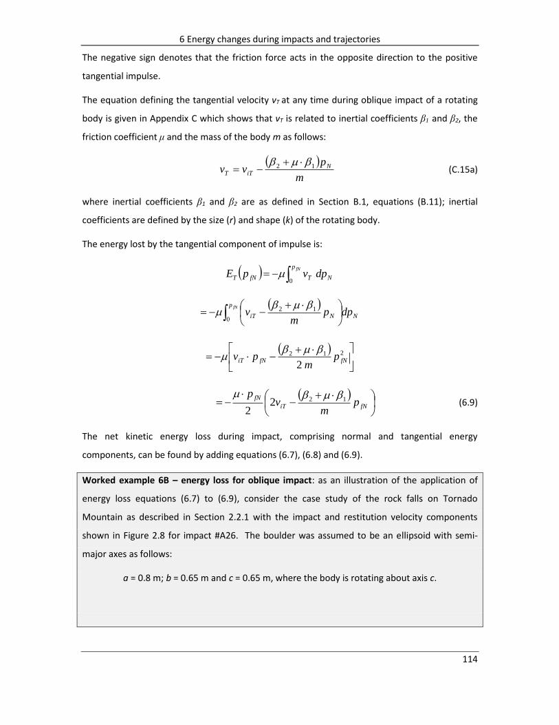
6 Energy changes during impacts and trajectories
114
The negative sign denotes that the friction force acts in the opposite direction to the positive
tangential impulse.
The equation defining the tangential velocity vT at any time during oblique impact of a rotating
body is given in Appendix C which shows that vT is related to inertial coefficients β1 and β2, the
friction coefficient μ and the mass of the body m as follows:
m
pvv N
iTT12
(C.15a)
where inertial coefficients β1 and β2 are as defined in Section B.1, equations (B.11); inertial
coefficients are defined by the size (r) and shape (k) of the rotating body.
The energy lost by the tangential component of impulse is:
fNp
NTfNT dpvpE0
fNp
NNiT dppm
v0
12
212
2fNfNiT p
mpv
fNiT
fNp
mv
p122
2
(6.9)
The net kinetic energy loss during impact, comprising normal and tangential energy
components, can be found by adding equations (6.7), (6.8) and (6.9).
Worked example 6B – energy loss for oblique impact: as an illustration of the application of
energy loss equations (6.7) to (6.9), consider the case study of the rock falls on Tornado
Mountain as described in Section 2.2.1 with the impact and restitution velocity components
shown in Figure 2.8 for impact #A26. The boulder was assumed to be an ellipsoid with semi-
major axes as follows:
a = 0.8 m; b = 0.65 m and c = 0.65 m, where the body is rotating about axis c.

6 Energy changes during impacts and trajectories
115
eN = 1.29eT = 0.27
viN = -4.4 m · s-1
vf = 6.4 m · s-1
vfT = 3.0 m · s-1
vfN = 5.7 m · s-1
θf = 63˚
ψslope = 25˚
θi = 22˚vi = 11.7 m · s-1
viT = 10.8 m · s-1 ·
Tree stumpheight = 1.4 m
-ω-ω
Detail of velocity componentsat impact point #A26 on colluvium
Figure 6.4: Translational and angular velocity components at impact point #A26 for Tornado Mountain rock fall event
The volume of the ellipsoid is 1.42 cu. m., and the mass is about 3750 kg if the rock unit weight
is 26 kN · m-3. The radius of gyration of the body k is ((a2 +b2)/5)1/2 = 0.46 m. The average radius
of the body is (a + b)/2 = 0.725 m.
The values of the three inertial coefficients are given by equations (B.11) as follows:
β1 = 1 + rb2/k2 = 3.00; β2 = ra rb/k2 = 2.46; β3 = 1 + ra
2/k2 = 4.02
For an impact velocity of vi = 11.7 m · s-1 at an angle θi = 22 degrees, the normal and tangential
components of the initial velocity are:
viN = -11.7 sin(22) = -4.4 m · s-1 and viT = 11.7 cos(22) = 10.8 m · s-1
For the granular colluvium on the slope surface at the impact point, the friction coefficient μ can
be assumed to have a value of 0.68, as determined in the laboratory testing carried out by
Masuya et al. (2001), and described in Section 5.3.
Substitution of these parameter values in equation (6.6) gives a value for the impulse at
maximum compression, pcN = 2898 kg · m · s-1. The calculated value of the normal coefficient of
restitution eN at impact #A26 is 1.30 (Figure 2.8), so the final impulse, pfN = pcN (1+eN) = 6665 kg ·
m · s-1.

6 Energy changes during impacts and trajectories
116
Using these values for impulses pfN and pcN, the changes in energy at impact #A26 are calculated
as follows:
EN(pc) = -12.9 kJ; EN(pf) - EN(pc) = 10.7 kJ; ET(pf) = -31.3 kJ
and the net energy loss during impact due to changes in translational velocities, is equal to the
sum of these energy changes, ΔE = is -33.5kJ.
6.2 Rotational energy gains/losses
The rotational energy Er of a falling body depends on its mass and shape as defined by its
moment of inertia I, and the angular velocity ω, as follows:
2
2
1 IEr (6.10)
As an example of measured angular velocities of rock falls, Section 3.4.1 (Figure 3.10) describing
the Ehime test site in Japan shows that ω first increases with the fall distance and then tends to
a terminal velocity in the range of about 15 to 35 rad · s-1. Furthermore, the angular velocity
may increase or decrease during impact depending on the geometry of the impact, so the
rotational energy may also increase or decrease during impact.
Based on equation (6.10), where the angular velocity changes from ωi at the point of impact to
ωf at the termination of impact, the change in rotational energy during impact is:
22
2
1fir IE (6.11)
Worked example 6C – change in rotational energy: as an illustration of the application of
equations (6.10) and (6.11), consider rock fall impact #A26 at Tornado Mountain discussed in
the previous section. This body was assumed to be an ellipsoid with semi-axes of a = 0.8 m, b =
0.65 m and c = 0.65 m, and mass, m of approximately 3750 kg. The moment of inertia of an
ellipsoid rotating about axis c is (see Table 4.1):
22
5ba
mI = 797 kg · m2 (6.12)
No measurements of the angular velocity are available for this fall. However, an approximate
value for the angular velocity can be obtained from equation (3.17) where a relationship

6 Energy changes during impacts and trajectories
117
between the angular velocity ω, the final translational velocity vf and the radius r of the body
has been developed from the measurements of the angular velocity of test rocks. That is,
r
v f
f (3.17)
If the radius r = 0.725 m, and the final translational velocity, vf(A26) = 6.4 m · s-1 (Figure 2.8), then
the final angular velocity, ωf(A26) = -8.8 rad · s-1.
The impact angular velocity at #A26, ωi(A26) is equal to the final angular velocity at impact point
#A25, equal to ωi(A25), because the angular velocity does not change during the trajectory from
#A25 to #A26. Trajectory calculations for the rock fall show that the final velocity at #A25 was
vf(A25) = 8.07 m · s-1, and from equation (3.17), ωi(A26) = -11.1 rad · s-1. Based on these translational
velocity parameters, the angular velocity decreased from -11.1 to -8.8 rad · s-1 during impact
#A26. From equation (6.11), the change in rotational energy during the impact is
2
1 rE 797( (-11.1)2-(-8.8)2 )
= - 18.3 kJ
6.3 Total energy losses
The total energy loss during impact is the sum of the translational and rotational energy losses.
Referring to the calculated energy losses for Tornado Mountain impact #A26 that are calculated
in Worked examples 6B and 6C above, the total energy loss is equal to:
ΔE = ΔKE + ΔRE = (-33.5) + (-18.3) = -51.8 kJ
These calculations show that the rotational energy loss is about 35 per cent of the total energy
loss; the field data (Chapter 2) shows that this ratio between the kinetic and rotational energies
is typical for rock falls.
The theoretical energy losses calculated using impact mechanics as described in Sections 6.1 and
6.2 and demonstrated in Worked examples 6A, 6B and 6C, can be compared with the change in
kinetic energy, ΔKE calculated from the initial and final velocities for impact #A26 as shown in
Figure 6.4 where vi = 11.7 m · s-1 and vf = 6.4 m · s-1.
22
2
1fi vvmKE = - ½ 3750 (11.72 – 6.42) = -180 kJ.
6 Energy changes during impacts and trajectories
118
These values for the theoretical and field net energy losses show that the theoretical value
calculated from impact mechanics theory is less than the actual energy losses. That is, for the
translational velocities, the theoretical energy loss is only 19 per cent (-33.5/-180 = 0.19) of the
actual energy loss, or for the combined kinetic and rotational energies, the theoretical energy
loss is about 29 per cent (-51.8/-180 = 0.29) of the field value. It is expected that this difference
is because the impact mechanics theory does not fully account for the plasticity that occurs in
actual rock fall impact, or the loss of mass due to fragmentation of the block (see Section 6.5).
For impacts in the other case studies described in Chapter 2, the theoretical energy losses are
also less than the actual energy losses, with the differences being similar to those for Tornado
Mountain impact #A26. Furthermore, the differences between the theoretical and actual
energy losses shows no apparent relationship to the type of slope material, although further
studies of the available data may provide information on a factor to be included in the energy
loss equations to account for the plastic deformation at the impact points.
6.4 Energy loss diagrams
One of the design requirements of rock fall protection structures is locating the structure where
the rock fall energy is at a relatively low value along the rock fall path. The general behavior of
rock falls with respect to energy changes during the series of impacts and trajectories is as
follows:
Potential energy (PE) will decrease continuously during the fall in proportion to the loss
of elevation;
Translational kinetic energy (KE) will decrease during impact in proportion to the
reduced velocity, as a result of compression of the slope material in the normal
direction, and frictional losses in the tangential direction;
Rotational energy (RE) may decrease or increase during impact depending on the
attitude of the body at the point of impact (see Figure 3.11);
Translational energy will increase during the trajectory phases of the fall as the result of
gravity acting on the body to increase the vertical velocity component;
Rotational energy will remain constant during trajectories because no rotational forces
act on the body when it is moving through the air.

6 Energy changes during impacts and trajectories
119
It is assumed that no energy losses due to air friction occur during trajectories because they
would be very small compared to impact energy losses. Also, gravity effects during impacts can
be ignored because reaction forces are large compared to the body force and act for a very
short time, and no significant change in the position of the body occurs during impact.
These energy changes during a rock fall can be illustrated on energy loss diagrams, of which two
types are discussed in the following sections.
6.4.1 Energy partition diagram for potential, kinetic and rotational energies
At the moment that a rock fall detaches from the slope, it will possess potential energy equal to
PE = m · g ·h (6.13)
where m is the mass of the body, g is the gravitational acceleration and h is the total fall height.
As the body falls during the first trajectory, the potential energy is converted into kinetic energy
that increases as the body accelerates. At the first impact point, the velocity decreases as the
slope deforms and the body slips, causing the kinetic energy to decrease. Also at the impact
point, the body starts to rotate and gain rotational energy as the result of friction forces acting
on the periphery of the body. Once the body leaves the slope, the translational velocity and
kinetic energy increase due to gravitational acceleration, while the angular velocity remains
constant. This sequence of events is repeated with each impact.
Figure 6.5 illustrates an energy partition diagram for a cubic concrete block at the Ehime test
site in which the PE, KE, RE are all represented at each every impact point and during each
trajectory. The vertical axis shows the overall vertical height of the fall from the source, with the
elevation of each impact point defined. The horizontal axis shows the partition of the energy
throughout the fall, with the maximum value equal to the potential energy at the source; the
potential energy decreases continually during the fall. At each impact point, the decrease in
velocity, and corresponding kinetic energy loss, is represented by the decrease in the width of
the KE area. The rotational energy area remains constant during trajectories, but for this test
the rotational energy increases with each impact as shown by the increase in width of the area
representing RE during impact. The relative widths of the KE and RE bands indicate the low ratio
between RE and KE.

6 Energy changes during impacts and trajectories
120
The area between the potential energy area and the combined kinetic-rotational area
represents the cumulative energy loss at the impact points that becomes wider with each
impact. All the energy has been dissipated when the rock stops moving.
The value of the energy partition diagram is that it enables low energy locations on the slope to
be identified that are the optimum locations for rock fall fences or barriers. That is, energy will
be high on the steep, upper part of the face but will diminish as the slope angle is reduced. Also,
the trajectories will be close to the ground on the lower slope, which will limit the height of
protection structures.
Another factor to consider in the location of fences or barriers is to find areas immediately after
an impact point where the kinetic energy has been lost during impact and before gravity has
caused the velocity to increase during the next trajectory. Impact points will often occur on
benches where rock falls accumulate.

6 Energy changes during impacts and trajectories
121
Figure 6.5: Energy loss diagram for cubic, concrete block with constant mass at Ehime test site, Japan – see Figure 2.6 (Ushiro et al., 2001)
6.4.2 Energy head
An alternative method of showing the progressive energy loss for a series of impacts is to plot
the “energy head”, given by:
g
vzE
2
2
(6.14)
where z is the body elevation and v is the length of the velocity vector (Hungr and Evans, 1988).
A plot of energy head comprises a horizontal line during each trajectory where the energy head

6 Energy changes during impacts and trajectories
122
is constant, and a drop in the energy head representing the loss of energy at each impact point.
Plots of this type have been used to show the transition from trajectory to rolling phase of rock
falls where the slope of the energy line equals the coefficient of rolling friction for the slope
material.
6.5 Loss of mass during impact
The energy change calculations discussed previously in this chapter all assume that the mass of
the rock fall remains constant throughout the fall. In reality, falls will break up to some extent at
the impact points so that the final mass will be less than the mass at the source. Possible
reasons for breakup of the body are that the initial block contains planes of weakness along
which fracture can readily occur during impact with the slope. Also, the initial body may have an
irregular form that will progressively break down into a more uniform spherical or ellipsoidal
shape that will spin and bounce more readily than an elongated shape.
Quantitative information on the loss of mass during the course of a rock fall can be obtained
from studies carried out in Italy (Nicolla et al., 2009), and from the Tornado Mountain rock fall
site described in Section 2.2.1. The Italian studies involved two natural rock fall sites where
previous events could be observed, as well as a test site where the falls were carefully
documented. These data have been used to develop a relationship between the body size and
the distance travelled from the source.
A summary of the two Italian rock fall sites and the Tornado Mountain case study described in
Chapter 2 is a follows:
Camaldoli Hill, Naples – the slope geometry at the rock fall locations comprised a 200 m
(660 ft) high upper rock slope at an overall angle of about 56 degrees, above a 60 m (200 ft)
high talus slope at an angle of 37 degrees. The maximum horizontal fall distance was about
200 m (660 ft). The rock forming the cliff is a tuff (Neapolitan yellow tuff) of varying
composition that had a uniaxial compressive strength up to about 10 MPa and deformation
modulus of about 10 GPa. The rock contains sets of sub-vertical joints that are parallel and
normal to the slope, and a sub-horizontal joint set that dips at 5 to 38 degrees and forms the
base of columnar blocks. The joint spacing has a maximum value of about 3 to 5 m (10 to 15
ft) which defines the maximum block size.

6 Energy changes during impacts and trajectories
123
Block sizes were assessed by mapping the dimensions of blocks in-place on the cliff face, and
of fallen blocks on the slope. A total of 298 blocks were mapped on the face with volumes
ranging from 1 cu. m (1.3 cu. yd) to 50 cu. m (65 cu. yd), with about 34 per cent of the blocks
having volumes less than 2.5 cu. m. (3.3 cu. yd). A total of 120 fallen blocks were mapped,
of which 96 per cent had volumes less than 5 cu. m (6.6 cu. yd) indicating the fragmentation
of blocks during falls.
In addition to the natural falls, a test was conducted on a slope with similar geometry where
images of the falls were analyzed to determine the approximate size of blocks before and
after impact. The initial volumes of the test blocks ranged from 1 to 12 cu. m (1.3 to 16 cu.
yd).
Monte Pellegrino, Palermo – the slope geometry comprised a 100 m (330 ft) high slope at a
face angle of about 42 degrees gradually flattening to a slope angle of 23 degrees; the
maximum vertical fall height was 290 m (950 ft) and the horizontal distance was about 300
m (980 ft). The rock forming the cliffs is a strong, blocky limestone with a compressive
strength of about 100 MPa and a modulus of about 100 GPa.
Similarly to the Camaldoli Hill site, block sizes were measured in situ and on the run-out
area. Most of the in situ blocks had volumes up to 2.5 cu. m (3.3 cu. yd), with the largest
volume being about 27 cu. m (35 cu. yd), while 87 per cent of the fallen blocks had volumes
of less than 5 cu. m (6.6 cu. yd).
Tornado Mountain, Canada – at this site where the two separate rock fall paths were clearly
distinguishable on the slope, it was possible to measure the final dimensions of the rock fall,
as well as fragments that had broken from the block at specific impact locations (see Figure
2.7). It was not possible to access the source area on a steep rock face to measure the
dimensions of the original rock falls. However, from observations of the size of the clearly
visible source area, and of the very strong, massive limestone forming the slope it is
estimated that the original rock falls had volumes in the range of 30 to 50 cu. m (40 to 65 cu.
yd).
The Italian field data were used to develop the following relationship between the volume of the
source rock fall Ω0, and the volume Ω at any horizontal distance x from the source:
x1
1
0
(6.15)

6 Energy changes during impacts and trajectories
124
where λ (m-1) is a reduction coefficient defining the loss of mass with distance fallen.
Figure 6.6 shows the values of the coefficient λ defining the envelopes of loss of mass data for
the Mt. Pellegrino and Camaldoli Hill rock fall sites. For the Mt. Pellegrino data, the values of λ
are in the range of 0.0035 and 0.01 m-1, while for the Camaldoli Hills, the values of λ values are
in the range of 0.008 to 0.02 m-1. These results demonstrate that as much as 80 per cent of the
original rock mass is lost during the course of the rock fall, with most of this loss probably
occurring in the first few impacts where the rock is falling fast down the steep face, and the
irregular shape is broken down at the impact points. Also, the initial impacts may be on the rock
face where more fragmentation may occur compared to the talus or soil lower on the slope.
Figure 6.6: Plot of horizontal rock fall distance x against loss of volume ratio, Ω/Ω0 showing ranges of values of λ for data from Mt. Pellegrino and Camaldoli Hills (Nicolla et al., 2009)
It is of interest that the limestone at Mt. Pellegrino is an order of magnitude stronger than the
tuff in the Camaldoli Hills and that the reduction in mass is less at Mt. Pellegrino than at the
Camaldoli Hills. These results indicate that the values of λ may have a relationship with the rock
strength.
For the Tornado Mountain rock fall site (see Section 2.2), the dimensions of selected rock
fragments broken off the main rock fall in the lower part of the slope were recorded, together
with the corresponding impact number. For rock fall A, where the final volume was about 1.42
cu. m (1.86 cu. yd) (mass = 3750 kg) (8,300 lb), it was estimated that fragments with a total
volume of about 8 cu. m (10.5 cu yd) broke off the body after impact #A10, of which a total of

6 Energy changes during impacts and trajectories
125
ten blocks with a total volume of about 2 cu. m (2.6 cu. yd) broke off between impacts #26 and
#31. It was not possible to distinguish rock fragments from above impact #A10, but it is
expected that much of the loss of volume occurred early in the fall where the rock fell 40 m (130
ft) on to a bare rock bench. Using this data, the following approximate relationship was
developed between the volume Ω(n) at impact number n, the initial volume Ω(0):
8.0
)0(
)(
n
n (6.16)
Equation (6.16) shows that if Ω(46) = 1.42 cu. m (2 cu. yd) after 46 impacts, then the original
volume Ω(0) was about 30 cu. m (40 cu. yd); a rock fall with this volume is feasible for this strong,
massive limestone. That is, about 95 per cent of the original rock volume was lost during this fall
over a total horizontal distance of about 610 m (2,000 ft).
In order to compare the results of equations (6.15) for the Italian data and (6.16) for the
Tornado Mountain events, the positions of the impacts at Tornado were converted into
horizontal distances from the source x, with the fall stopping at a distance of x = 610 m (2,000
ft), and the ratio Ω/Ω0 = 1.42/30 = 0.047. Substitution of these values into equation (6.15) gives
a value for the reduction coefficient λ, of 0.03, and a curve on slightly below those show on
Figure 6.6. It is considered that this value for λ is consistent with the Italian data considering the
relatively limited information available at Tornado Mountain.
The loss of volume (and mass) during the course of rock falls obviously has an effect on the
potential, kinetic and rotational energy losses. While the energy partition diagram in Figure 6.5
shows the loss of energy for each impact at the Ehime test site for a constant mass, Figure 6.7
shows the loss of energy for the mass decreasing at each impact point according to the
relationship given in equation (6.15).
The test block was a cubic-shaped concrete body with side dimensions of 0.6 m (2 ft), and an
initial volume, Ω0 = 0.22 m3 (0.30 yd3) (mass = 520 kg) (1150 lb), and the total horizontal (x)
distance travelled was 57 m or 190 ft (Figure 2.6). Assuming a reduction factor of λ = 0.02, the
decrease in volume is calculated using equation (6.15), for a final volume of 0.1 m3 (0.1 yd)3.
Figure 6.7 shows details of the changes in potential, kinetic and rotational energy for the fall at
the Ehime test site in Japan described in Section 2.2 for a mass that reduces with each impact
according to equation (6.15), from an initial volume of 0.22 m3 (0.3 yd3) to a final volume of 0.1

6 Energy changes during impacts and trajectories
126
m3 (0.13 yd3). In preparing the plot shown in Figure 6.7, the calculated progressively reduced
mass at each impact during the fall was used to calculate the corresponding reduced values of
the potential and kinetic energies, as well as the reduced moment of inertia of the body to
calculate the changes in rotational energy (see equation (6.10)). For a cubic body with side
length L, the moment of inertia, I is given by (see Table 4-1):
6
2LmI
Figure 6.7: Energy partition plot for diminishing mass at the Ehime rock fall test site – cubic concrete block with initial side length 0.6 m (2 ft)

6 Energy changes during impacts and trajectories
127
Comparison of the two sets of energy partition lines shown in Figures 6.5 and 6.7 clearly
demonstrate the effect of the rock mass diminishing during the fall, assuming that the
translational velocities at the impact points are the same for each case. The increased width of
the energy loss area on Figure 6.5 compared to Figure 6.7 represents the energy required to
fracture the falling rock.
An application of the concept of rock mass loss during falls, is in the design of rock fall fences.
For a fence located at some distance from the source, the impact energy will be less than for a
fence located close to the source.
6.6 Effect of trees on energy losses
Rock falls often occur on forested slopes because falls occur in wet, cold climates that are
conducive to tree growth, and falls are triggered by water and ice pressures. Also, growth of
tree roots in cracks can be a triggering mechanism as discussed in Section 1.4.
Studies have been carried out in both Japan (Masuya, et al., 2009; Ushiro et al., 2006) and
Europe (Dorren and Berger, 2012; Dorren, Berger and Putters, 2006; Dorren and Berger, 2005)
to quantify the effect of trees on rock fall behavior. The Japanese tests by Ushiro were part of
the Ehime study (see Section 2.1) where fall velocities and run-out distances were measured for
tests conducted before and after the trees were removed. At Ehime, the talus was sparely
forested with pine and oak having trunk diameters in the range of 100 to 500 mm (4 to 20 in).
Measurements of impact velocities showed no significant difference in the velocities between
tests conducted with the trees on the slope and after they were removed. Similar results were
obtained at Tornado Mountain where the impacted trees were about 200 mm (8 in) in diameter.
Where trees were impacted by rock falls, they were sheared off with apparently no reduction in
the velocity of the fall; Figure 2.7 shows a typical tree on Tornado Mountain that was impacted
and sheared off by a rock fall.
Masuya et al. (2009) have developed a rock fall simulation model that incorporates the tree
height, trunk diameter and a probability density function expressed as the number of trees per
square meter of slope surface. Collisions between a rock and a tree are modeled in the same
manner as collisions with the slope, but with a restitution coefficient of 0.1 and a friction
coefficient of 0.03. The model showed that the effect of trees is to approximately halve the
velocity of the falls, and to cause a wider dispersion of the falls on the slope compared to a bare
slope. Section 3.5.3 discusses dispersion areas of rock falls on talus slopes.

6 Energy changes during impacts and trajectories
128
In the European study by Dorren and Berger (2005), tests were conducted on two similar parts
of a talus cone with a slope angle of 38 degrees and a slope length of 302 m (990 ft). One part
of the talus was denuded of trees, while the other part was forested with trees having an
average diameter of 310 mm (12 in) and density of 290 trees per hectare. This slope
configuration allowed two near identical rock fall tests to be conducted – one slope with trees
and one without trees. For each test, 100 rocks were rolled with their impacts and trajectories
recorded at 25 frames per second by five high speed cameras mounted in nearby trees; the
rocks had an average diameter of 0.91 m (3 ft) and volume of 0.49 cu. m (0.6 cu. yd). The effect
of the trees on the rock fall behavior was to reduce the average velocity from 13.4 m · s-1 (44 ft ·
s-1) to 11.2 m · s-1 (37 ft · s-1), and the maximum velocity from 14.8 m · s-1 (49 ft · s-1) to 11.6 m · s-
1 (38 ft · s-1). From these results, as well as other tests on the resistance of trees to impact, it
was possible to find a relationship between the diameter of tree trunks (measured at chest
height, approximately where impacts occur), and the energy dissipated per tree for six tree
species as shown in Figure 6.8. The tests also showed the relative wider dispersion of the rock
falls by the tree impacts compared to bare slopes, similarly to that modeled by Masuya (2009).
Figure 6.8: Relationship between maximum energy that can be dissipated by six different tree species and the tree diameter, measured at chest height (Dorren and Berger, 2005)
The energy dissipation data shown on Figure 6.8 can be used to evaluate the results obtained
from the Ehime test site and the Tornado Mountain rock fall events. In both these cases, the
tree diameters were in the range of 100 to 200 mm (4 to 8 in) where the energy dissipation

6 Energy changes during impacts and trajectories
129
would be negligible. This low energy dissipation is consistent with the observation that the tree
impacts at Ehime and Tornado Mountain had no significant effect on rock fall velocities and run-
out distance.
Another characteristic of tree impact observed by Dorren and Berger is for rocks that are
entirely or partially stopped by a tree. In some of these cases, the “whipping” action of the tree
during impact can break off the upper part of the tree well above the impact point. Figure 6.9
shows a cedar tree with a diameter of 1.1 m (3.6 ft) that stopped a rock with a volume of about
5.5 cu. m (190 cu. ft.) moving at an estimated velocity of 5 to 10 m s-1 (15 to 30 ft · s-1); the
approximate impact kinetic energy was 200 to 800 kJ (80 to 300 ft tonf). The tree was tilted and
broke off at a height of about 14 m (46 ft) above the ground. Comparison of these impact
parameters with Figure 6.8 confirms the capacity of this 1.1 m diameter tree to absorb this
impact energy.

6 Energy changes during impacts and trajectories
130
Figure 6.9: Impact of a 5 cu. m (6.5 cu. yd) rock fall with kinetic energy of about 200 to 800 kJ (75 to 300 ft tonf) with a 1.1 m (3.6 ft) diameter cedar tree. Rock was stopped and upper part of tree was broken off about 14 m above base (Vancouver Island, near Ucluelet)

7 Rock fall modeling
131 131
7 Rock fall modeling
Design of rock fall protection structures requires information on the mass and impact velocity of
the fall to determine the impact energy, and the fall trajectories to determine the height and
location of the structure on the slope. These design parameters are usually obtained from
computer simulation programs. Numerous modeling programs have been developed since the
late 1980’s that include programs, and a variety of university research tools. The complexity of
these programs varies from simple two-dimensional, lumped mass models, to three-dimensional
models in which the shape and size of the body can be defined and its orientation is tracked
during the fall.
This chapter discusses first, the general principles of rock fall modeling, the required input
parameters and the outputs that are generated. Second, analysis results are presented that
model the rock falls for the five case studies described in Chapter 2; the modeling was carried
out using the RocScience program Rocfall 4.0. The purpose of carrying out these back analyses
was to determine the values of the input parameters that are required to closely model the
actual events. It is intended that these analyses will provide benchmarks for rock fall modeling,
because comparisons of the results of rock fall analysis programs with commonly used
parameters show that calculated trajectories are often higher than those that occur in the field.
The consequence of unrealistically high, calculated trajectories is that many fences and barriers
are higher, and more expensive, than required. For example, the author has observed fences
that were designed using commercial software, where all the impacts were in the lower one
third of the structure.
Another purpose of providing the case study information in Chapter 2 is to provide actual rock
fall data that can be used by developers of modeling software to calibrate their programs.
The modeling methods discussed in this chapter are based on the programs RocFall 4.0
(RocScience, 2012) and CRSP – Colorado Rockfall Simulation Program (Pfeiffer and Higgins
(1995); Jones, et al., (2000)). These two programs are commercially available and the
calculations methods are documented in detail. Also, the two programs can produce identical
results with the use of appropriate input parameters. Figure 7.1 shows the results of a typical
rock fall simulation for the Mt. Stephen site using RocFall 4.0 (Section 2.1.1).

7 Rock fall modeling
132
a)
b)
Rock (strong limestone)
Rn 0.75
Rt 0.59
Φ 5.71° SD 2.5°
Roughness SD 11.5
70 80 90 100 110 12060
40
30
20
10
0
Ele
va
tio
n, z –
co
ord
ina
tes (
m)
50
Off-set, x - coordinate (m)
MSE wall
H = 6.6 m
Steel wire fence
H = 5.0 m
a)
b)
Rock (strong limestone)
Rn 0.75
Rt 0.59
Φ 5.71° SD 2.5°
Roughness SD 11.5
70 80 90 100 110 12060
40
30
20
10
0
Ele
va
tio
n, z –
co
ord
ina
tes (
m)
50
Off-set, x - coordinate (m)
MSE wall
H = 6.6 m
Steel wire fence
H = 5.0 m
Rock (strong limestone)
Rn 0.75
Rt 0.59
Φ 5.71° SD 2.5°
Roughness SD 11.5
70 80 90 100 110 12060
40
30
20
10
0
Ele
va
tio
n, z –
co
ord
ina
tes (
m)
50
Off-set, x - coordinate (m)
MSE wall
H = 6.6 m
Steel wire fence
H = 5.0 m
Figure 7.1: Rock falls at Mt. Stephen (see section 2.1). a) Simulation of rock falls showing three typical rock fall paths; b) accumulation of falls that impacted fence on top of barrier
7.1 Spreadsheet calculations
A detailed analysis of rock fall trajectories and impacts for a lumped mass can be carried out on
a spreadsheet using the basic principles of trajectories and impact mechanics described in the
previous chapters. The calculation method is summarized in this section.
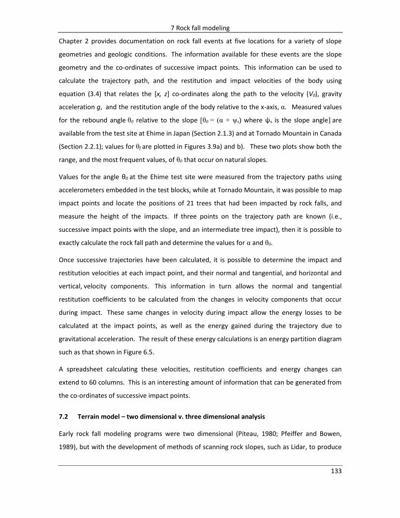
7 Rock fall modeling
133
Chapter 2 provides documentation on rock fall events at five locations for a variety of slope
geometries and geologic conditions. The information available for these events are the slope
geometry and the co-ordinates of successive impact points. This information can be used to
calculate the trajectory path, and the restitution and impact velocities of the body using
equation (3.4) that relates the [x, z] co-ordinates along the path to the velocity (V0), gravity
acceleration g, and the restitution angle of the body relative to the x-axis, α. Measured values
for the rebound angle θ0 relative to the slope [θ0 = (α + ψs) where ψs is the slope angle] are
available from the test site at Ehime in Japan (Section 2.1.3) and at Tornado Mountain in Canada
(Section 2.2.1); values for θf are plotted in Figures 3.9a) and b). These two plots show both the
range, and the most frequent values, of θ0 that occur on natural slopes.
Values for the angle θ0 at the Ehime test site were measured from the trajectory paths using
accelerometers embedded in the test blocks, while at Tornado Mountain, it was possible to map
impact points and locate the positions of 21 trees that had been impacted by rock falls, and
measure the height of the impacts. If three points on the trajectory path are known (i.e.,
successive impact points with the slope, and an intermediate tree impact), then it is possible to
exactly calculate the rock fall path and determine the values for α and θ0.
Once successive trajectories have been calculated, it is possible to determine the impact and
restitution velocities at each impact point, and their normal and tangential, and horizontal and
vertical, velocity components. This information in turn allows the normal and tangential
restitution coefficients to be calculated from the changes in velocity components that occur
during impact. These same changes in velocity during impact allow the energy losses to be
calculated at the impact points, as well as the energy gained during the trajectory due to
gravitational acceleration. The result of these energy calculations is an energy partition diagram
such as that shown in Figure 6.5.
A spreadsheet calculating these velocities, restitution coefficients and energy changes can
extend to 60 columns. This is an interesting amount of information that can be generated from
the co-ordinates of successive impact points.
7.2 Terrain model – two dimensional v. three dimensional analysis
Early rock fall modeling programs were two dimensional (Piteau, 1980; Pfeiffer and Bowen,
1989), but with the development of methods of scanning rock slopes, such as Lidar, to produce

7 Rock fall modeling
134
digital terrain models (DTM) ) it has become possible to import DTM’s into rock fall modeling
programs and run three dimensional analyses.
Modeling of a slope in two dimensions will only provide reliable results if the cross section is
reasonably uniform along the slope. However, as discussed in Section 3.5.1, it is found that rock
falls often accumulate in gullies in a similar manner to which water flows down slopes. Figure
3.12 shows a slope in which all the rock falls over a slope length of several hundred meters along
the crest are concentrated in three narrow gullies. Modeling of rock falls on this slope using a
two dimensional program would give erroneous results because the model would not simulate
the sinuous shape of the gullies and the generally uniform slope profile along the path of the
gullies. A two dimensional analysis of the slope in Figure 3.12 would show a series of ridges and
hollows that would not be realistic model of the rock fall path.
7.3 Modeling methods – lumped mass
The primary components of rock fall modeling programs are first, algorithms to calculate the
rock fall impacts and trajectories and second, routines to process the graphics of the slope and
the rock fall paths. Of these components, the calculation of the impacts and trajectories can be
readily accomplished if a lumped mass model is used, as is the case with the programs RocFall
4.0 and CRSP; the calculations can be handled on a spreadsheet as described in Section 7.1.
However, the calculations are more complex if the shape and size of the body are defined such
that the program tracks the orientation of the body during both the trajectory and impact
phases of the fall. Still more complexity is introduced if the rock breaks up during impact.
This section reviews the methods used to calculate trajectories and impacts for a lumped mass
model such as used in the programs RocFall 4.0 and CRSP. Section 7.4 discusses models that use
bodies with defined dimensions and shapes.
The component of the modeling programs that processes the graphics is beyond the scope of
this thesis.
7.3.1 Rock fall mass and dimensions
The lumped mass model , which is used in the programs RocFall 4.0 and CRSP, assumes that the
body is infinitely small, which allows the use of Newtonian mechanics as described in the earlier
chapters, to calculate impact and trajectory behavior, ignoring the effect of air friction. The
mass of the body is used to determine energies from the calculated velocities, and it is assumed

7 Rock fall modeling
135
that the mass is constant during the fall; loss of mass during the course of a fall is discussed in
Section 6.5.
Calculation of the effects of slope roughness (see Section 7.3.6) and rotational velocity (see
Section 7.3.7) requires a value for the dimensions of the body. In CRSP, the default body shape
is a sphere, because it yields the maximum volume for a given radius, and the program
calculates the radius of the body from the mass and rock density. It is also possible to define
cylindrical and discoid shaped bodies in order to calculate corresponding moments of inertia.
7.3.2 Slope definition parameters
Development of a rock fall model requires definition of the slope parameters that comprise the
slope geometry, and the material properties. The slope geometry is defined, for a two-
dimensional model, by a series of [x - z] co-ordinates that join straight line segments. Each
segment is assigned a slope material, the properties of which are the normal and tangential
coefficients of restitution, the surface roughness and the friction angle. These parameters are
discussed in the following sections.
Some models use a “spline” function to create a smooth curved surface between the defined
points, but this approach does not allow a series of horizontal benches and steep cut slopes to
be modeled.
7.3.3 Rock fall seeder
The rock fall models incorporate a “seeder” that defines the rock fall conditions at the origin of
the falls in the model. In RocFall 4.0, the seeder parameters are the horizontal and vertical
translational velocity components, the rotational velocity and the mass of the fall. These
parameters allow falls to be modeled either where the source of the falls is the same point as
the seeder (vx = vz ≈ 0), or where the source of the falls is outside the model area and the falls
have finite velocities at the origin of the model (vx , vz > 0). The relative values of vx and vz are
selected to obtain the required trajectory angle.
With respect to angular velocity, either a negative or positive value can be input. However, it
appears that the direction of rotation makes little difference to the calculated trajectories.
Typical RocFall 4.0 analyses show that the effect of rotational velocity is to flatten trajectories,
which is consistent with impact mechanics theory for negative direction of rotation (see Section
4.6.4 and Figure 4.9).

7 Rock fall modeling
136
7.3.4 Normal coefficient of restitution
The coefficient of restitution, e relates the velocity of the falling body at the end of impact with
the velocity at the moment of impact (see Chapter 4). It is also usual to examine the velocity
changes in the normal (N) and tangential (T) components of velocity during impact and the
corresponding normal eN, and tangential eT, coefficients of restitution. This section discusses the
normal coefficient, while Section 7.3.5 discusses the tangential coefficient and its relationship to
the frictional properties of the slope surface.
The normal coefficient of restitution is defined as follows:
iN
fN
Nv
ve (4.6)
where vfN is the normal component of the velocity at the completion of the impact (t = f), and viN
is the normal component of velocity at the moment of impact (t = i).
It is recognized in the CRSP and RocFall 4.0 models that eN is not a material property, but is
dependent on impact conditions and to a lesser degree on the type of slope material. That is,
for a high velocity impact the body will tend to penetrate further into the ground in an inelastic
impact, compared to a lower velocity impact that will tend to be a more elastic and have a
greater rebound height. This behavior is modeled by the following empirical equation that
scales the normal component of the restitution velocity vfN, according to the following equation:
2
1K
v
evv
iN
NiNfN (7.1)
where viN is the normal component of the impact velocity, and K is a constant. The term
[(1+(viN/K)2)-1] is a scaling factor that is equal to 0.5 for the default value of K = 9.14 m · s-1 (30 ft ·
s-1). Figure 7.2 is a plot of the scaling factor given by equation (7.1) for values of K ranging from
9 to 40 m · s-1 (30 to 130 ft · s-1). The curves show that vfN equals viN (i.e., eN = 1) for low velocity
impacts when the scaling factor approaches 1 for elastic impact.

7 Rock fall modeling
137
Figure 7.2: Plot of normal component of impact velocity and scaled normal coefficient of restitution from equation (7.1)
The form of the relationship given by equation (7.1) and plotted in Figure 7.2 is similar to that
discussed in Section 5.2.1 and in Figure 5.5 that relates the normal coefficient of restitution eN to
the impact angle θi. That is, high normal velocities occur when the impact is close to normal, or
θi > ~60 degrees. Under these conditions, eN has a low value close to the basic coefficient of
restitution determined by a drop test (see Figure 5.6). However, for shallow impacts where θi <
~30 degrees and the normal velocity component is small, the value of eN becomes larger.
Equation (7.1) shows that the maximum value of eN scaled is 1.0, while the field data and impact
mechanics show that eN can have values greater than 1 for shallow impact angles. The
relationship between θi and eN is given by the equation:
03.15.19
iNe (5.4)
7.3.5 Tangential coefficient of restitution and friction
The tangential coefficient of restitution eT, is defined by the ratio of the final and initial
tangential velocities during impact as follows:
iT
fT
Tv
ve (4.7)
Tangential velocity changes depend on the extent of slip and rolling that occurs during impact,
and the effects of friction at the rock-slope contact.

7 Rock fall modeling
138
In CRSP, the tangential coefficient of restitution is scaled by a friction factor f(F), and a scaling
factor SF that incorporate the impact translational and rotational velocities, and the normal
coefficient of restitution (Pfieffer and Bowen, 1989). In RocFall 4.0, analysis values for eT
incorporate data from back analysis of rock falls.
Since eT is related to a effective friction coefficient μ’, guidance on appropriate values for eT can
be obtained from measurements of fall velocity related to the fall height and the slope angle
(Japan Road Association, 2000); Table 3.1 lists values for μ’ for characteristics of different slope
materials. For example, μ’ ≈ 0.05 for “smooth, strong rock surfaces with no tree cover”, and μ’
≈ 0.35 for “talus with angular boulders exposed at the surface, no tree cover”. In addition,
values for eT have been calculated by back analysis for the five case studies discussed in Chapter
2 and are listed in Table 2-1; these values have been used in the RocFall 4.0 modeling of these
five sites as presented in Section 7.5.
In RocFall 4.0, the friction angle φ input parameter is related to calculate the distance that the
body slides down the slope when the trajectory phase of the fall is complete. The value of φ
used in the analysis is a function of the body shape since a spherical body will have less frictional
resistance to sliding than a tabular body. The distance L that a body will slide along a surface
dipping at ψs degrees and with a friction angle φ is:
tancossin2
22
ss
fTiT
g
vvL (7.3)
where viT is the tangential velocity at the start of sliding and vfT is the velocity when the body has
slid distance L (Stevens, 1998).
7.3.6 Surface roughness
The surface roughness of the slope materials has a significant effect on rock fall behavior, i. e.,
trajectory heights generally increase with increased roughness.
Surface roughness can be quantified by relating the perpendicular variation s, of the slope from
the average slope inclination, within a slope distance equal to the radius r, of the body (Pfieffer
and Bowen, 1989) as shown in Figure 7.3. The angle ε is defined by the dimensions r and s as
follows:
r
s1tan (7.4)

7 Rock fall modeling
139
Figure 7.3 shows that the value of the angle ε diminishes with increasing radius of the body.
That is, for approximately the same slope roughness, the roughness angle will diminish as the
body size increases, (r1 > r2) and (ε2 > ε1).
In CRSP, the slope roughness is input as the dimension s from which the angle ε is calculated
using the defined radius of the spherical body. In RocFall 4.0, the roughness is defined as a
standard deviation in the dip angle of the slope segment.
Figure 7.3: Relationship between slope roughness (ε) and radius of rock fall (r)
7.3.7 Rotational velocity
Rock falls rotate as the result of the moment generated by the tangential velocity and the
frictional resistance at the contact of periphery of the body and the slope surface. Rotation of
the body has two main effects on rock fall behavior. First, rotation causes the trajectories to be
flatter than for a non-rotating body (see Section 4.6.4), and second, the rotating body has
rotational energy that contributes to the total impact energy (see Section 6.2).

7 Rock fall modeling
140
Body rotation is incorporated in the CRSP and RocFall 4.0 models by calculating the rotational
velocity ω for a body with radius r with tangential translational velocity vT from the following
relationship:
r
vT (7.5)
The rotational energy (RE) of the body can be calculated using the moment of inertia, I, for the
selected body shape and the calculated rotational velocity (RE = ½ I · ω2).
7.3.8 Probabilistic analysis
Modeling of rock falls must take into account the natural variability of site conditions that
includes irregularly shaped blocks of rock, and variability of the coefficients of restitution and
slope roughness. Actual site conditions are modeled by probabilistic analyses in which the
average input parameters include standard deviations that represent the likely range of the
parameter values from the average values. The program then carries out a Monte Carlo analysis
for a large number of rock fall runs, with a random number generator selecting parameter
values for each run from the probability distributions defined by the standard deviations. The
result of the Monte Carlo analysis is a plot of all the analyzed rock falls that shows the likely
distributions of rock fall behavior that may be expected.
Examples of probabilistic analyses are provided in Section 7.5 for the five case studies described
in Chapter 2.
7.3.9 Data sampling points
The usual objective of running rock fall models is to design structures and ditches to protect
facilities at the base of the slope. Design information required for these structures are the
trajectory height and the impact energy. The modeling programs incorporate sampling points at
which information is provided on distributions of analysis data – total, translational and
rotational energies, velocity and trajectory height. By moving the sampling point across the
slope, it is possible to identify the location with the minimum energy and/or the lowest
trajectory.
Examples of data generated at sampling points are provided in the analyses of the case studies
in Section 7.5.

7 Rock fall modeling
141
7.4 Modeling methods – discrete element model (DEM)
Rock falls models that use a lumped mass in which the mass of the body is defined but the mass
is concentrated in a point are described in Section 7.3. Alternatively, discrete element models
(DEM) can be used in which the mass, dimensions and shape of the body are defined, and the
body can break into smaller fragments as it impacts the slope during the fall (Zhang and Rock,
2012) (Chen et al., 2013).
In DEM analysis, the body is made up of a collection of small spheres, in tight tetrahedral
packing, connected with appropriate constitutive models to describe rigidity, heterogeneity and
fracture of the model. This model can accurately replicate trajectories, rolling, sliding, launching
behavior of the body, and crack propagation within the body. With respect to impact of the
body with the slope, the parameters related to impact that are required for DEM modeling are
damping, stiffness and friction coefficients.
As of 2013, commercial modeling programs in which the mass, shape and size of the body are
defined are not widely available.
7.5 Modeling results of case studies
For each of the five documented rock fall sites described in Chapter 2, a computer simulation
has been run using the program Rocfall 4.0 (RocScience, 2012). These analyses demonstrate the
operation and results of the program, and determine the site parameters that are required to
produce calculated rock fall paths that closely follows the actual paths.
In defining the modeling parameters required to duplicate the actual field results, it was found
that very fine adjustments were necessary in the average values of parameters. That is,
analyses of active rock fall sites using apparently appropriate input parameters may show that
falls stop part way down the slope, or that unrealistically high trajectories are generated.
7.5.1 Rock fall model of Mt. Stephen events
Section 2.1.1 in Chapter 2 describes the rock fall conditions at Mt. Stephen in the Rocky
Mountains near Field, British Columbia in Canada. Figures 2.1 and 2.2 show respectively
photographs of a portion of the site, and a typical section of the lower part of the slope. This is
a highly active rock fall site, due to the topography, geology and weather. That is, the mountain
is about 2000 m (6550 ft) high at an overall face angle of about 50 degrees so that rock falls can
fall from great heights and attain high velocities, with most falls reaching the base of the slope.

7 Rock fall modeling
142
The geology comprises horizontally bedded limestone and shale where the limestone is much
stronger than the shale and occurs in thicker beds; the limestone contains sets of vertical joints.
The relatively rapid weathering of the shale compared to the limestone results in the formation
of unstable overhangs and columns in the limestone that are the sources of the rock falls. The
other factor causing the high rock fall frequency is the weather – very cold winters forming ice
on the slope, and rainfall during the spring and fall. Figure 7.4 shows the lower 120 m (400 ft)
portion of the slope.
The protection provided for these severe rock fall and snow avalanche conditions comprises a
6.6 m (21.5 ft) high MSE (mechanically stabilized earth) wall, with a 5 m (16.5 ft) high steel wire
fence along the top (Figure 7.1). This barrier has been very successful in protecting the railway
from both types of hazard.
The actual rock falls at Mt. Stephen have been modeled using the program RocFall 4.0. Figure
7.4 shows the calculated trajectories for three falls, and Figures 7.5 and 7.6 show graphs of the
distributions of impact location, velocity and energy at the barrier location
The material types used in the analysis was rock for the entire slope, with soil in the ditch
behind the barrier. For this case study, all the rock falls were contained by the barrier so it was
not possible to use the back analysis feature in RocFall 4.0. The parameters for the slope,
including the standard deviations (SD) quantifying the range of the values, required to simulate
the rock falls are shown in Figure 7.4. It is assumed that all rock falls originated higher on the
slope than elevation 118 m (390 ft.) so the x and z seeder velocities have values that generate
trajectories that are consistent with observed field conditions.

7 Rock fall modeling
143
20 40 60 80 100 1200
80
60
40
20
0
Point seeder
X velocity 11 m/s SD 3.0
Z velocity 6 m/s SD 2.5
Rock mass 44 kg
ω -20 rad/s SD 3.0
Off-set, x – coordinate (m)
Ele
va
tio
n, z –
co
ord
ina
te (
m)
140
100
120
Rock (strong limestone)
Rn 0.75
Rt 0.59
Φ 5.71° SD 2.5°
Roughness SD 11.5
Analysis point
x = 116.3
Figure 7.4: Simulation of rock falls at Mt. Stephen for three calculated rock trajectories
Observations of rock fall impacts on the MSE barrier and the fence provided reliable information
on the impact locations. In total, it was possible to identify 466 impact points as either chips on
the concrete blocks forming the face of the MSE wall, or as deformations of the steel wires in
the fence. Analysis of the impact locations showed their vertical distribution, with impacts over
the full 11.6 m (38 ft) height of the structure with the maximum impacts at the base and the
number of impacts decreasing with height. The horizontal distribution of impacts showed that
most occurred where the slope geometry included the lower face sloping at about 45 degrees
on which many blocks impacted and then generated a trajectory that impacted the barrier
(Figure 7.4). Figure 7.5 shows the calculated vertical distribution of the impacts on the barrier,
which closely match the actual impact locations.
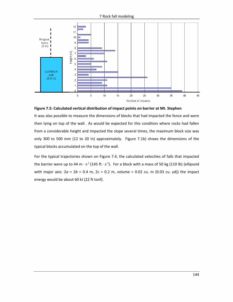
7 Rock fall modeling
144
Figure 7.5: Calculated vertical distribution of impact points on barrier at Mt. Stephen
It was also possible to measure the dimensions of blocks that had impacted the fence and were
then lying on top of the wall. As would be expected for this condition where rocks had fallen
from a considerable height and impacted the slope several times, the maximum block size was
only 300 to 500 mm (12 to 20 in) approximately. Figure 7.1b) shows the dimensions of the
typical blocks accumulated on the top of the wall.
For the typical trajectories shown on Figure 7.4, the calculated velocities of falls that impacted
the barrier were up to 44 m · s-1 (145 ft · s-1). For a block with a mass of 50 kg (110 lb) (ellipsoid
with major axis: 2a = 2b = 0.4 m, 2c = 0.2 m, volume = 0.02 cu. m (0.03 cu. yd)) the impact
energy would be about 60 kJ (22 ft tonf).

7 Rock fall modeling
145
Figure 7.6: Analysis using RocFall 4.0 of rock falls at Mt. Stephen at barrier, analysis point x = 116.3 m a) translational velocity distribution; b) total energy (KE + RE) distribution
The calculated velocities and energies plotted in Figure 7.6 appear to be less than the actual
values where falls originate on the steep slope from heights of hundreds of meters above the
barrier and attain high velocities.
7.5.2 Rock fall model of Kreuger Quarry, Oregon tests
The purpose of the rock fall tests carried out in the Krueger Quarry in Oregon was to determine
the required dimensions and configurations of catchment areas to contain rock falls on
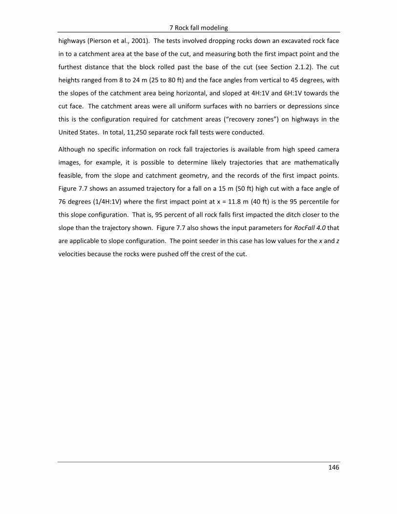
7 Rock fall modeling
146
highways (Pierson et al., 2001). The tests involved dropping rocks down an excavated rock face
in to a catchment area at the base of the cut, and measuring both the first impact point and the
furthest distance that the block rolled past the base of the cut (see Section 2.1.2). The cut
heights ranged from 8 to 24 m (25 to 80 ft) and the face angles from vertical to 45 degrees, with
the slopes of the catchment area being horizontal, and sloped at 4H:1V and 6H:1V towards the
cut face. The catchment areas were all uniform surfaces with no barriers or depressions since
this is the configuration required for catchment areas (“recovery zones”) on highways in the
United States. In total, 11,250 separate rock fall tests were conducted.
Although no specific information on rock fall trajectories is available from high speed camera
images, for example, it is possible to determine likely trajectories that are mathematically
feasible, from the slope and catchment geometry, and the records of the first impact points.
Figure 7.7 shows an assumed trajectory for a fall on a 15 m (50 ft) high cut with a face angle of
76 degrees (1/4H:1V) where the first impact point at x = 11.8 m (40 ft) is the 95 percentile for
this slope configuration. That is, 95 percent of all rock falls first impacted the ditch closer to the
slope than the trajectory shown. Figure 7.7 also shows the input parameters for RocFall 4.0 that
are applicable to slope configuration. The point seeder in this case has low values for the x and z
velocities because the rocks were pushed off the crest of the cut.

7 Rock fall modeling
147
2 4 8 10 12 140
8
6
4
2
0
Point seeder
X velocity 0.17 m/s
Z velocity 0.47 m/s
Rock mass 580 kg
Rock (strong basalt)
Rn 1.00
Rt 0.59
Φ 3.01° SD 3.01°
Roughness SD 5
Ditch
Rn 0.25
Rt 0.59
Φ 3.01° SD 3.01°
Roughness SD 5
10
12
14
16
6 16 18 20
Off-set, x – coordinate (m)
Ele
va
tio
n, z –
co
ord
ina
te (
m)
Analysis point
x = 10.0
95 percentile:
1st impact
x = 11.895 percentile:
Roll out
distance
x = 19.4
Figure 7.7: Calculated trajectories for two 580 kg (1,280 lb) rocks at Krueger Quarry rock fall tests on 15 m (50 ft) high cut at a face angle of 76 degrees; refer to Fig 10.3 for first impact and roll out distances
Figure 7.7 also shows an analysis point located at x = 10 m (33 ft), or about 1.4 m (5 ft) from the
base of the cut; this location represents the 70th percentile of the first impact points. The
calculated distributions of translational velocities and energies at x = 10 m (33 ft) are shown on
Figure 7.8.

7 Rock fall modeling
148
Figure 7.8: Analysis using RocFall 4.0 of rock falls at Krueger Quarry for 15 m (50 ft) high cut at a face angle of 76 degrees, analysis point x = 10 m (33 ft) a) translational velocity distribution; b) total energy (KE + RE) distribution
7.5.3 Rock fall model of Ehime, Japan test site
In 2003 a series of rock fall tests was carried out at a test site in Ehime Prefecture on Shikoku
Island in Japan, as part of an extensive testing program that started in about 1961, located at
least 16 other sites around Japan (see Sections 2.1.3 and 2.2.1). The Ehime tests were
comprehensive in terms of the number of block shapes tested and the range of site conditions,
and were documented in detail using 14 high speed cameras on the slope, and accelerometers

7 Rock fall modeling
149
sampling at 2 kHz embedded in concrete blocks. The data collected allowed the precise
positions of impact points and trajectory paths to be determined throughout each fall, as well as
the translational and rotational velocities.
The test slope was a 42 m (140 ft) high natural slope, comprising a 26 m (85 ft) high rock face at
an angle of 44 degrees in horizontally bedded sandstone and shale, with a 16 m (50 ft) high talus
slope forming the lower part of the slope. The talus cone was sparsely vegetated with pine and
oak trees with trunk diameters of 100 to 200 mm (4 to 8 in).
The test conditions were as follows. The test bodies comprised concrete cubes – side length 0.6
m (2 ft) and weight of 520 kg (1,150 lb), concrete spheres – diameter 0.54 m (1.8 ft) and weight
of 200 kg (440 lb), and blocks of rock with masses ranging from 120 kg to 2060 kg (260 to 4550
lb). The tests involved rolling ten cubes, ten spheres and 20 blocks of rock, with half the tests
being run on the natural treed slope, and the second half after the trees had been removed.
The collected data was used to determine the fall paths and trajectory heights, as well as the
translational and rotational velocities. A photograph of the slope is shown in Figure 2.5, and
details of the interpreted data are presented in Figure 3.5 – trajectory heights normal to the
slope; Figure 3.6 – translational velocities; Figure 3.9 distribution of restitution angles; and
Figure 3.10 – angular velocities.
Figure 7.9 shows a simulation, using RocFall 4.0, of the actual fall path of a concrete cube as
shown on Figure 2.6. The input parameters for the rock and talus material properties and the
seeder values are also shown on Figure 7.9.

7 Rock fall modeling
150
10 20 30 40 50 600
40
30
20
10
0
Point seeder
X velocity 0 m/s
Z velocity 0 m/s
Rock mass 520 kg
Rock (sandstone & mudstone)
Rn 1.00
Rt 0.59
Φ 8.53° SD 2°
Roughness SD 3
Talus
Rn 1.00
Rt 0.72
Φ 19.29° SD 2°
Roughness SD 8
Off-set, x – coordinate (m)
Ele
vati
on
, z –
co
ord
inate
(m
)
Analysis point
x = 52.1
10 20 30 40 50 600
40
30
20
10
0
10 20 30 40 50 600
40
30
20
10
0
Point seeder
X velocity 0 m/s
Z velocity 0 m/s
Rock mass 520 kg
Rock (sandstone & mudstone)
Rn 1.00
Rt 0.59
Φ 8.53° SD 2°
Roughness SD 3
Talus
Rn 1.00
Rt 0.72
Φ 19.29° SD 2°
Roughness SD 8
Off-set, x – coordinate (m)
Ele
vati
on
, z –
co
ord
inate
(m
)
Analysis point
x = 52.1
Figure 7.9: Calculated trajectory using RocFall 4.0 for a 520 kg (1150 lb) concrete cube at the test site in Ehime Prefecture in Japan
Figure 7.10 shows a comparison between the actual and calculated trajectory heights for a test
with a concrete cube. The two sets of data are reasonably consistent except for the talus impact
at x = 34 m where the calculated trajectory is 50 per cent greater than the actual trajectory.
Figure 3.5 shows the measured trajectory heights for all the tests, where 99 per cent of the
trajectory heights were less than 2 m (7 ft), and 95 per cent were less than 1.5 m (5 ft).

7 Rock fall modeling
151
Figure 7.10: Trajectory height envelope comparison between field results and RocFall 4.0 simulated results for concrete cube at test site in Ehime Prefecture in Japan
Figure 7.11 shows the distributions of the velocity and total energy of 24 tests of concrete
cubes. The analysis point (x = 52.1 m) is located at the base of the talus slope where a rock fall
protection structure may be located. The calculated velocities at the analysis point can be
compared with the actual velocities at this location shown on Figure 3.6. Where H = 41 m in
Figure 2.6, equivalent to x = 52.1 m in Figure 7.9, the actual range of velocities is 5 to 15 m·s-1.
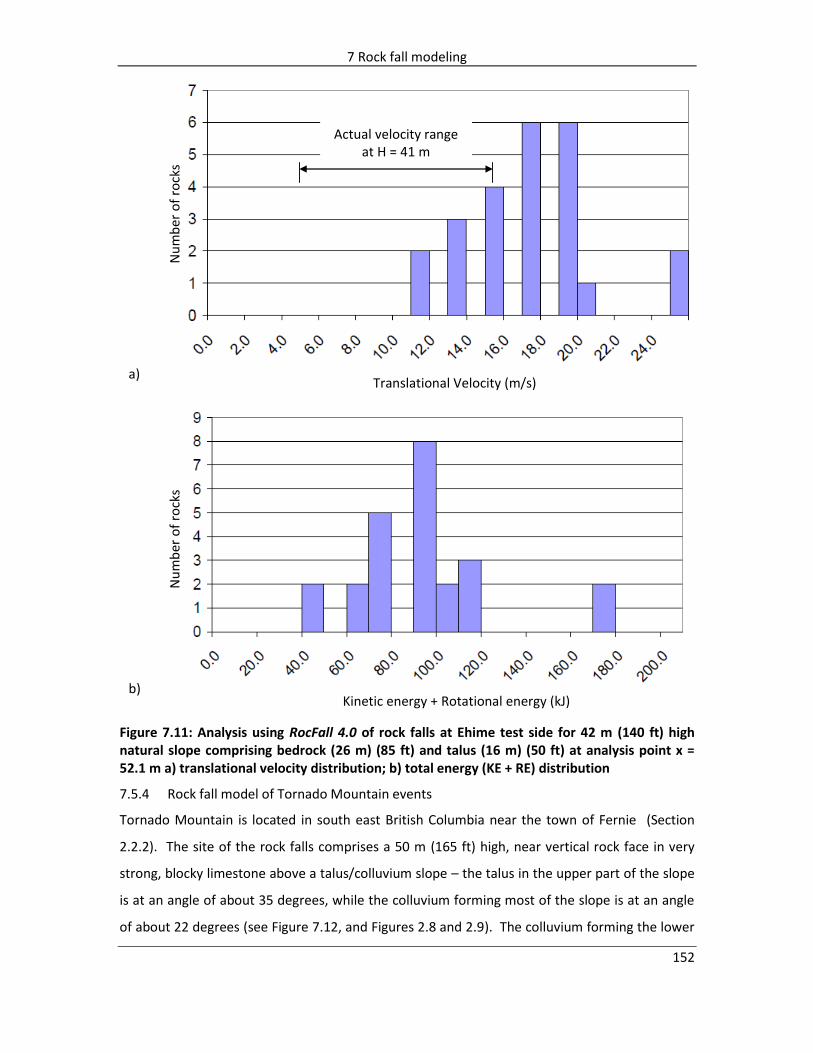
7 Rock fall modeling
152
a)
b)
a)
b)
Translational Velocity (m/s)
Kinetic energy + Rotational energy (kJ)
Nu
mb
er o
f ro
cks
Nu
mb
er o
f ro
cks
Actual velocity range at H = 41 m
Figure 7.11: Analysis using RocFall 4.0 of rock falls at Ehime test side for 42 m (140 ft) high natural slope comprising bedrock (26 m) (85 ft) and talus (16 m) (50 ft) at analysis point x = 52.1 m a) translational velocity distribution; b) total energy (KE + RE) distribution
7.5.4 Rock fall model of Tornado Mountain events
Tornado Mountain is located in south east British Columbia near the town of Fernie (Section
2.2.2). The site of the rock falls comprises a 50 m (165 ft) high, near vertical rock face in very
strong, blocky limestone above a talus/colluvium slope – the talus in the upper part of the slope
is at an angle of about 35 degrees, while the colluvium forming most of the slope is at an angle
of about 22 degrees (see Figure 7.12, and Figures 2.8 and 2.9). The colluvium forming the lower

7 Rock fall modeling
153
slope is a mixture of gravel and soil forming a uniform slope with no significant irregularities; the
slope is sparsely vegetated with trees having diameters ranging from about 300 to 500 mm (12
to 20 in).
In 2004, two separate rock falls, with masses of A = 3750 kg (8,300 lb) and B = 5600 kg (12,400
lb), occurred from a source area on the limestone cliff. The rocks travelled total distances of 740
m (2450 ft) down the slope before impacting a horizontal bench where most of the kinetic
energy was absorbed and the rocks stopped within 30 m (100 ft). Because the two rocks
followed slightly different paths and no previous falls had occurred in this area, it was possible
to identify and map most of the impact points in the slope, including 21 trees that were sheared
off by the falls. This information on the impact locations allowed velocities and trajectories to
be calculated as discussed in Section 2.2.2.
Figure 7.12 shows the results of the RocFall 4.0 simulation of Tornado Mountain fall A, with the
input parameters required to produce trajectories that reasonably closely match the field
measurements. Figure 7.13 compares the calculated trajectory heights with the average height
measured in the field of 1.5 m (5 ft) and shows that most of the calculated trajectories are
significantly higher than actual heights. This discrepancy between calculated and actual heights
can lead to the construction of protection structures that are higher than required. It is the
author’s experience that calculated trajectories are often higher than actual trajectories.

7 Rock fall modeling
154
100 200 300 400 500 6000
400
300
200
100
0
Point seeder
X velocity 0 m/s
Z velocity 0 m/s
Rock mass 3750 kg
Rock (strong limestone)
Rn 0.75
Rt 0.59
Φ 2.86° SD 1.50°
Roughness SD 35
Off-set, x – coordinate (m)
Ele
vati
on
, z –
co
ord
inate
(m
)
Colluvium
Rn 1.00
Rt 0.62
Φ 19.29° SD 2°
Roughness SD 0
Analysis point
x = 610.0
Figure 7.12: Calculated trajectories using RocFall 4.0 for fall A, a 3750 kg (8300 lb) limestone block at Tornado Mountain
Figure 7.13: Trajectory height envelope from RocFall 4.0 simulated results for a 3750 kg (8300 lb) limestone block at Tornado Mountain

7 Rock fall modeling
155
Figure 7.14: Analysis using RocFall 4.0 of rock falls at Tornado Mountain, block A at analysis point x = 610 m a) translational velocity distribution; b) total energy (KE + RE) distribution
Figure 7.14 shows the calculated distributions for the velocity and energy at an analysis point
located just above the bench on which the railway is sited, and where a fence or barrier would
likely be constructed. The actual impact properties of fall A at this location were a velocity of 18
m · s-1 (60 ft · s-1) and a kinetic energy of 600 kJ (220 ft tons). If the block has a moment of
inertia of 800 kg · m2 and is rotating at 15 rad · s-1, then the rotational energy, RE = (½ I · ω2) = 90

7 Rock fall modeling
156
kJ, and the total energy is 690 kJ (255 ft tonf). These actual impact velocity and energy values
are plotted on Figure 7.14, showing that they are at the low end of the calculated distributions.
The comparatively high calculated velocities may account for the calculated trajectories being
higher than the actual trajectories.
7.5.5 Rock fall model of asphalt impact event
A single rock fall occurred from the crest of a natural 138 m (450 ft) high slope made up of a 56
m (180 ft) high rock slope at an angle of 60 degrees, a 70 m (230 ft) high colluvium slope at an
angle of 42 degrees, and a 10 m (33 ft) high rock cut above a highway (see Section 2.3). Figure
7.15 shows two calculated trajectories for the full fall height, together with the RocFall 4.0
parameters required to generate this simulation.
Figure 7.16 shows the calculated distributions of impact velocity and energy just before the
impact with the asphalt at the analysis point x = 140 m. These calculated values can be
compared with the precise trajectory of the fall from the crest of the rock cut to just before and
after impact with the asphalt as shown in Figure 2.10 and discussed in Section 2.3. For a block
with a mass of 500 kg (1100 lb), a moment of inertia, I = (m · k2) = (500 · 0.2952) = 43.5 kg · m2,
an impact velocity of 21.5 m · s-1 (70 ft · s-1), and a rotational velocity of 15 rad · s-1, the impact
kinetic and rotational energies are 115 kJ (42.5 ft tonf) and 4.8 kJ (1.8 ft tonf) respectively.
These actual velocity and energy values are plotted on the calculated distributions.
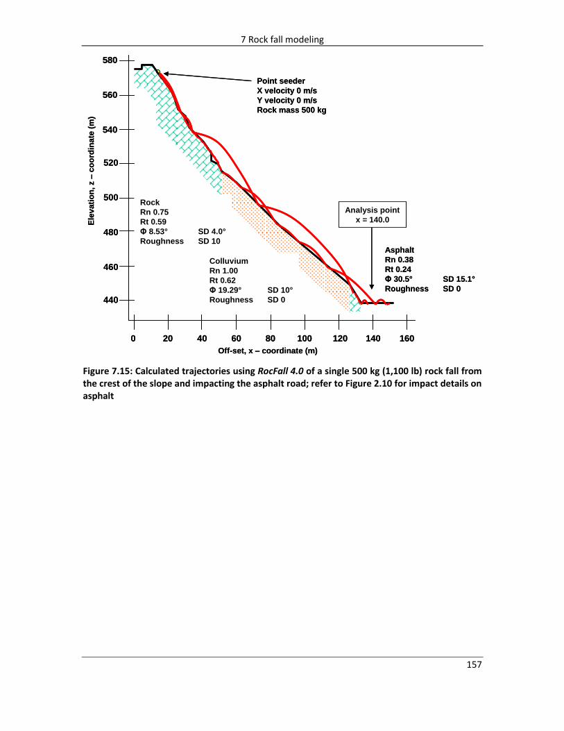
7 Rock fall modeling
157
20 40 60 80 100 1200
520
500
480
460
440
Point seeder
X velocity 0 m/s
Y velocity 0 m/s
Rock mass 500 kg
Off-set, x – coordinate (m)
Ele
va
tio
n, z –
co
ord
ina
te (
m)
140
540
560
160
580
Colluvium
Rn 1.00
Rt 0.62
Φ 19.29° SD 10°
Roughness SD 0
Analysis point
x = 140.0
Rock
Rn 0.75
Rt 0.59
Φ 8.53° SD 4.0°
Roughness SD 10Asphalt
Rn 0.38
Rt 0.24
Φ 30.5° SD 15.1°
Roughness SD 0
Figure 7.15: Calculated trajectories using RocFall 4.0 of a single 500 kg (1,100 lb) rock fall from the crest of the slope and impacting the asphalt road; refer to Figure 2.10 for impact details on asphalt

7 Rock fall modeling
158
Figure 7.16: Analysis using RocFall 4.0 of rock fall impacting asphalt at analysis point x = 140 m a) translational velocity distribution; b) total energy (KE + RE) distribution
7.6 Summary of rock fall simulation results
Section 7.5 describes the results of rock fall simulations for the five case studies described in
Chapter 2. The simulations show the calculated trajectory heights and the velocity and energy
distributions at selected analysis points that correspond to locations where reliable field data is
available. It was found that it is possible to simulate actual field conditions, although calculated
trajectory heights and velocities tend to be higher than actual heights and velocities.

7 Rock fall modeling
159
Furthermore, it was found that the calculated results are very sensitive to the input parameters.
Table 7-1 lists the input parameters that were used in the simulations, RocFall 4.0.
As a general comment on the simulation of rock falls, it is difficult to obtain calculated results
that are close to actual conditions without first knowing the actual field conditions in order to
calibrate the calculations. That is, small changes in the input parameters can produce large
changes in the calculated results that may appear to be reasonable, but are in fact incorrect. It
is hoped that the simulation results presented in this chapter will be of assistance in producing
reliable simulations.
Table 7-1: Summary of input parameters used in RocFall 4.0 to stimulate case study rock falls
Site no. Rock fall site
Slope material
Normal coefficient of restitution, eN
mean*
Tangential coefficient of restitution, eT
mean*
Friction Angle (deg)
mean / SD
Slope Roughness
(deg) SD
1 Mt. Stephen,
Canada rock 0.75 0.59 5.71 / 2.50 11.50
2 Oregon ditch study (rock
face impact) rock 1.00 0.59 3.01 / 3.01 5.00
2 Oregon ditch study (ditch
impact) rock 0.25 0.59 3.01 / 3.01 5.00
3 Ehime, Japan (rock slope)
rock 1.00 0.59 8.53 / 2.00 3.00
3 Ehime, Japan (talus slope)
talus 1.00 0.72 19.29 / 2.00 8.00
4 Tornado
Mountain, Canada
rock 0.75 0.59 2.86 / 1.50 35.00
4 Tornado
Mountain, Canada
colluvium 1.00 0.62 19.29 / 2.00 0.00
5 Highway asphalt 0.38 0.24 30.5 / 15.10 0.00
5 Highway rock 0.75 0.59 8.53 / 4.00 10.00
5 Highway colluvium 1.00 0.62 19.29 / 10.00 0.00
*In RocScience 4.0, default SD for eN and eT = 0.04

8 Design principles of rock fall protection structures
160 160
8 Design principles of rock fall protection structures
The design of rock fall protection structures such as wire rope fences is based on the efficient
absorption of impact energy. This requires that the structure be both flexible and stiff. That is,
the structure must be flexible to deflect during impact, and also stiff so that energy is absorbed
during deflection. The most effective protection structures are those in which energy is
absorbed uniformly throughout the impact period. This chapter discusses the design principles
for protection structures that absorb energy efficiently.
8.1 Structure location with respect to impact points
One of the factors in the location of protection structures is to find a position where the rock fall
energy is relatively low. That is, in order to limit the impact energy on the structure, it should be
located just after an impact point to benefit from the loss of energy due to plastic deformation
that occurs during the time that the rock is in contact with the ground.
Energy loss during impact can be demonstrated for rock falls at the Ehime test site in Japan. For
one of the tests, Figure 2.6 shows the impact and restitution velocities at each impact and the
energy partition plot in Figure 6.5 shows the corresponding kinetic and rotational energies over
the full extent of the rock fall path. The energy partition plot shows how the kinetic energy
increases due to gravitational acceleration during the trajectories and is lost during the impacts,
while the rotational energy changes (either increases or decreases) during the impacts, but
remains constant during the trajectories. For impact #5 at a fall height of 15.5 m (50 ft), the
impact kinetic energy is 53.4 kJ (20 ft tonf) while the restitution kinetic energy is 24.5 kJ (9 ft
tonf), a loss of 28.9 kJ (11 ft tonf) or 54 per cent during impact.
While this energy loss demonstrates the value in locating the structure immediately after impact
points, the generally uniform slope topography at the Ehime test site means that impacts will
not occur at well-defined locations on the slope. Therefore, no optimum location for a barrier
on the slope can be found.
A common topographic feature that defines an impact point along a rock fall path is a break in
slope forming a relatively shallow angle bench on which rock falls will tend to accumulate. If
such a feature does not occur naturally, it may be worthwhile to excavate a bench on which to

8 Design principles of rock fall protection structures
161
locate the barrier since it could be designed for a lower impact energy than one located on the
uniform slope.
For the rock fall site at Tornado Mountain discussed in Section 2.2.2 and shown in Figure 2.8, an
8 m (25 ft) wide bench was excavated in the slope on which the railway was constructed; Figure
8.1 shows a detail of the bench. Both the documented rock falls at the site impacted this bench
and stopped within 30 m (100 ft) of the railway after falling over a slope distance of about 700 m
(2,300 ft) down the uniform slope above the railway.
Trajectory calculations for Boulder A show that for rock falls impacting the horizontal bench
(impact #A43), the impact velocity was 17.9 m · s-1 (60 ft · s-1) and the restitution velocity was 9.8
m · s-1 (30 ft · s-1), representing a loss of kinetic energy of 422 kN (50 tonf) for the 3750 kg (8270
lb) block (i.e., KEA43i = 0.5 · 3750 · 17.922 = 602 kJ and KEA43f = 0.5 · 3750 · 9.82 = 180 kJ). That is,
70 per cent of the impact energy was lost during impact #A43, whereas for impacts on the more
uniform slope higher on the mountain, the typical energy loss was about 20 per cent. This
demonstrates the effectiveness of a horizontal bench on mitigating rock fall hazards - for a fence
or barrier located along the outer edge of such a bench, the design energy can be 50 per cent of
the energy required on the uniform slope.
Figure 8.1: Tornado Mountain rock fall site – for impact #A43 on 8 m (25 ft) wide bench excavated for the railway, 70 per cent of the impact energy is lost during impact
8.2 Attenuation of rock fall energy in protection structures
Figure 8.2 illustrates two examples of rock fall barriers - a flexible wire rope fence that has been
effective in stopping and containing rock falls, and a rigid concrete wall that has been shattered

8 Design principles of rock fall protection structures
162
by a rock fall. This section demonstrates how protection structures can be designed to
attenuate and dissipate a portion of the impact energy rather absorb the entire energy, and how
impact mechanics can be used to develop these designs.
Figure 8.2: Behavior of flexible and rigid structures. a) Flexible steel cable net that stops rock falls by deflection with no plastic deformation of the steel; b) rigid concrete wall shattered by rock fall impact
8.2.1 Velocity changes during impact with a fence
If a rock fall is stopped by a protection structure, then all the impact energy is absorbed in the
structure because the impact translational and rotational velocities are reduced to zero.
However, if the rock is redirected by the structure, then the restitution velocities have finite
values and the difference between the impact and restitution velocities represents the portion
of the impact energy absorbed in the structure (Figure 8.3).

8 Design principles of rock fall protection structures
163
vi
vi = 22 m/s
vf = 11.4 m/s
+ωivi
vf
μpN
+ωi
vi
μpN
θi
θi
PostNet
+N
T+
+N
T+
a)
b)
Hinge
Guy wire
with brake
+N
T+
Guy wire
with brake
Efficiency = Ef / Ei = 0
Efficiency = Ef / Ei
= 39 / 139 = 28 %
Figure 8.3: Effect of impact angle with fence on energy absorption. a) Normal impact results in the fence absorbing all impact energy; b) oblique impact results in rock being redirected off the net with partial absorption of impact energy
Figure 8.3 shows a rock fall fence on a slope at two orientations – normal to the slope (Figure
8.3a), and inclined up-slope (Figure 8.3b). The fence is impacted by a rock fall with initial
translational velocity vi and rotational velocity ωi, at an impact angle of the rock with the net of
θi.
For the fence oriented normal to the slope, the rock impacts the net approximately at right
angles (θi = 90 degrees). Under these conditions, the rock deflects the net and its velocity
progressively diminishes until it is reduced to zero at the point of maximum deflection before it
rebounds off the net. At the time of zero velocity, all the impact energy has been absorbed by
the net.

8 Design principles of rock fall protection structures
164
In contrast to the normal impact shown in Figure 8.3a), Figure 8.3b) shows the fence oriented
up-slope so that the rock fall impacts the net at an oblique angle (θi < 90 degrees). For this
impact angle, the rock is redirected by the net and the velocity decreases to vf when it loses
contact with the net; at no time during the impact does the velocity become zero. For these
conditions, only a portion of the impact energy is absorbed by the fence.
The behavior of a rotating body impacting a net at either a normal or oblique angle as shown in
Figure 8.3 can be modeled approximately using the principles of impact mechanics discussed in
Chapter 4. That is, equations (4.20) to (4.24) can be used to calculate the influence of the fence
configuration on changes in the translational and angular velocities and angles during impact.
For impact of a rotating body with a stationary net, the parameters governing the impact
behavior are the normal coefficient of restitution eN , the radius of the body r, and its radius of
gyration, k. In addition, the calculations require that normal and tangential axes be set up, with
the positive directions of each defined, as well as the impact and restitution angles of the
velocity vectors relative to the fence. Figure 8.3 shows these axes relative to the fence, with the
positive normal axis (+N) in the opposite direction to the impact direction, and the positive
tangential axis (+T) in the downward direction. This means that the normal component of the
impact velocity, which is towards the net, is negative (-vi). The orientations of the impact (i) and
restitution (f) velocity vectors – θi and θf – are defined relative to the fence inclination.
The insets on Figure 8.3 show the usual direction of rotation (clockwise) for rock falls due to the
frictional forces acting at the contact point with the slope (see Section 4.5). Since the direction
of rotation at the contact point is in the direction of the positive tangential axis, the clockwise
rotation is defined as a positive rotational velocity. The combined effect of the rotation and
normal impulse pN is to generate a frictional force (μ · pN) at the contact point that modifies the
shear component of the velocity and the restitution angle as discussed in Section 4.5.
Worked example 8A below shows the method of calculating the restitution velocities of a rock
fall impacting a fence at an oblique angle using equations (4.20) to (4.24) that apply impact
mechanics to model velocity changes during impact.
Worked example 8A – velocity changes during oblique impact: for oblique impact of a body
with a fence at the orientation shown in Figure 8.3b). The values for the impact parameters are:
vi = 22 m · s-1; ωi = 18 rad · s-1; θi = 50 degrees

8 Design principles of rock fall protection structures
165
The body is assumed to be a cube with side length of 0.6 m (see Section 2.1 on Ehime test site,
Japan), the properties of which are:
mass, m = 520 kg; radius (diagonal) = 0.43 m; radius of gyration, k = 0.35 m
For this impact geometry, the impact normal (N) and tangential (T) velocity components are as
follows:
viT = vi cos θi = 22 cos 50 = 14.1 m · s-1
and
viN = -vi sin θi = -22 sin 50 = -16.9 m · s-1
The final tangential velocity component is calculated using equation (4.20):
2
2
1k
r
rvvv iiT
iTfT
(4.20)
= 9.9 m · s-1
The final normal velocity is calculated using the normal coefficient of restitution, eN.
NiNfN evv = - (-16.9 · 0.35) = 5.9 m · s-1 (4.21)
where eN is defined by the impact angle θi as demonstrated in Section 5.2.2 and Figure 5.7.
Equation (5.4); approximately relates eN and θi as follows:
03.15.19
iNe (5.4)
Therefore, for an impact angle of 50 degrees, the approximate normal coefficient of restitution
is 0.35.
The final rotational velocity is given by equation (4.22):
2
22 1k
r
rv
k
r iiTif
(4.22)
= -11.6 rad · s-1
The final restitution velocity vf and angle θf can be calculated from the final tangential and
normal velocities components as follows:

8 Design principles of rock fall protection structures
166
22
fNfTf vvv = 11.5 m s-1 (4.23)
and
fT
fN
fv
vtana (4.24)
= 31 degrees
On Figure 8.3b), the velocity vectors are drawn to scale to show the results of the impact
calculations. These calculations show that the redirection of the body by the net results in the
velocity being reduced by 48 per cent, from vi = 22 m · s-1 to vf = 11.5 m · s-1. The velocity will
decrease up to the point of maximum deflection and will not be zero at any time.
The change in the rotational velocity from ωi = +18 rad · s-1 to ωf = -11.6 rad · s-1 indicates that
the direction of rotation reverses during impact. Model tests of bodies impacting the net at an
oblique angle indicate the reversal of the rotation direction.
8.2.2 Energy changes during impact with a fence
The velocity changes during impact with the fence discussed in Section 8.2.1 above and shown
in Figure 8.3 can also be used to calculate the energy changes during impact and determine how
much of the energy is absorbed by the net.
For the fence configuration shown in Figure 8.3a) where the impact is normal to the net, the
velocity of the rock is reduced from the initial velocity vi at the moment of impact to zero at the
time of maximum deflection. Therefore, the total impact energy of the rock fall is absorbed by
the net, i.e. (E = ½ m · vi2). This type of impact is also illustrated in Figure 8.2a) where the rocks
that have been stopped by the net accumulate in the base of the fence.
For the fence configurations shown in Figures 8.3b) and 8.4 where the impact is oblique to the
net, the velocity decreases during impact but the rock is not stopped. Therefore, only a portion
of the impact energy is absorbed by the fence, with the remainder of the energy being retained
by the moving rock.
Worked example 8B below illustrates the calculation method for an oblique impact with a fence.

8 Design principles of rock fall protection structures
167
Worked example 8B – energy changes during oblique impact: calculations of the velocity
changes that occur during an oblique impact are described in Worked example 8A. The
corresponding energy changes during impact are calculated as follows.
For an oblique impact of 50 degrees with the net, the velocity decreases from 22 m · s-1 to 11.5
m · s-1, and the rotational velocity changes during impact from 18 rad · s-1 to -11.6 rad · s-1.
The moment of inertia of the body, I = m · k2 = 520 · 0.352 = 63.7 kg · m2
Assuming that the mass of the rock remains constant during impact, the initial and final energies
are as follows:
Initial energy: KEi = ½ m· Vi2 = ½ 520 · 222 = 125.8 kJ; REi = ½ I · ωi
2 = ½ 63.7 · 182 = 10.3 kJ
Total impact energy, Ei = (125.8 + 10.3) = 136.1 kJ
Final energy: KEf = ½ m · Vf2 = ½ 520 · 11.52 = 34.4 kJ; REf = ½ I · ωf
2 = ½ 63.7 · (-11.6)2 = 4.3 kJ
Total final energy, Ef = (34.4 + 4.3) = 38.7 kJ
These calculations show that, for an oblique impact, the impact energy that is absorbed by the
net is 97.4 kJ (136.1 – 38.7), which is only 72 per cent of the impact energy compared to 100 per
cent of the impact energy for a normal impact.
8.2.3 Energy efficiency of fences
The discussion on the velocity and energy changes related to the impact configuration in
Sections 8.2.1 and 8.2.2 above can be used to quantify the relationship between energy
absorption by the fence and the impact configuration.
For a normal impact where the rock fall is stopped by the net, all the impact energy is absorbed
by the structure, which has to be designed to withstand the full impact energy. In contrast, for
an oblique impact only a portion of the impact energy is absorbed by the structure. The portion
of the impact energy that is deflected by the net can be expressed in terms of the efficiency of
the structure as follows:
%E,energypactIm
E,energystitutionReE,Efficiency
i
f
e 100 (8.1)

8 Design principles of rock fall protection structures
168
For the two fence configurations shown in Figures 8.3a) and b), the efficiencies are respectively
0 per cent for the normal impact and Ee = 39.2/138.8 = 28 per cent for the oblique impact where
the rock fall is redirected by the net.
The benefit of a high efficiency fence is that, for the same impact energy, it can be constructed
from lighter weight materials than a zero efficiency fence. Conversely, design impact loads will
be greater with increasing energy efficiency of the fence. The influence of fence configuration
on energy efficiency is discussed further in Section 8.3 and 8.4 of this chapter.
8.2.4 Configuration of redirection structures
Figure 8.3 shows how an oblique impact on a net can be achieved by inclining the fence up-
slope. The same impact configuration occurs for the hanging net shown in Figure 8.4 where a
vertical hanging net, that is unconstrained along its lower edge, is suspended from a series of
posts attached to the rock face. When rock falls impact the net, their velocity is reduced and
they are redirected into a catchment area at the base of the net; the rock falls that accumulate
in the catchment area can be readily removed by maintenance equipment. In comparison, for
the net shown Figure 8.2a) removal of accumulated rock falls requires access of the slope to
detach the lower edge of the net from the support cables.
The hanging net configuration shown in Figure 8.4 is applicable at locations where the rock face
is near vertical and the ditch width is limited so that it is not possible to construct the type of
fence shown in Figure 8.2a).

8 Design principles of rock fall protection structures
169
vi
Post
Hanging
netHinge
Guy wire
with brake
Figure 8.4: Hanging net installed on steep rock face that redirects rock falls into containment area at base of slope, where cleanout of accumulated rock falls is readily achieved
8.2.5 Hinges and guy wires
Both the fence configurations shown in Figures 8.3b) and 8.4 incorporate hinges at the base of
the posts, and guy wires, equipped with brakes, to hold the posts in place. These two
components of the fences are energy absorbing features that, together with the net itself,
ensure that the entire structure is flexible. Ideally, all components of the fence are equally
flexible because forces tend to concentrate in the stiffest part of the structure. The absorption
of impact energy with time in rock fall containment structures is discussed in Section 8.3, with
the design objective being to absorb energy uniformly during impact in order to minimize the
forces induced in the structure.
Commercially available braking elements in the guy wires, comprising a variety of loops, coils or
sliding connections, that absorb energy by plastic deformation and need to be replaced when
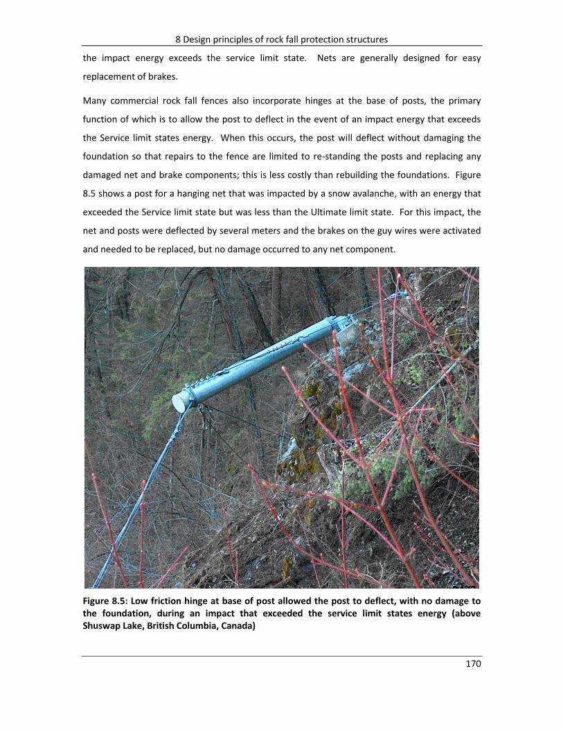
8 Design principles of rock fall protection structures
170
the impact energy exceeds the service limit state. Nets are generally designed for easy
replacement of brakes.
Many commercial rock fall fences also incorporate hinges at the base of posts, the primary
function of which is to allow the post to deflect in the event of an impact energy that exceeds
the Service limit states energy. When this occurs, the post will deflect without damaging the
foundation so that repairs to the fence are limited to re-standing the posts and replacing any
damaged net and brake components; this is less costly than rebuilding the foundations. Figure
8.5 shows a post for a hanging net that was impacted by a snow avalanche, with an energy that
exceeded the Service limit state but was less than the Ultimate limit state. For this impact, the
net and posts were deflected by several meters and the brakes on the guy wires were activated
and needed to be replaced, but no damage occurred to any net component.
Figure 8.5: Low friction hinge at base of post allowed the post to deflect, with no damage to the foundation, during an impact that exceeded the service limit states energy (above Shuswap Lake, British Columbia, Canada)

8 Design principles of rock fall protection structures
171
In contrast to the energy absorbing features of brakes, most hinges are low friction units that do
not absorb energy when the post deflects. It is believed that inclusion of frictional elements into
hinges will allow the hinges to both deflect in order to prevent damage to the foundation, and
to absorb energy. The combined activation of the guy wire brakes and the post frictional hinges
will produce a reasonably uniform absorption of energy during the time of impact. As discussed
in Section 8.3 below, uniform energy absorption with time minimizes the forces that are induced
in the fence by the impact.
8.3 Minimizing forces in rock fall protection fences
A fundamental design feature of effective rock fall fences and barriers is the flexibility of the
structure so that energy is absorbed in the structure during impact. An example of a flexible
structure is a net fabricated with woven steel wires that is supported on posts with flexible
hinges and deformable guy wires; most components of the net will deform and absorb energy
with impact (Figure 8.2a)). This energy absorption will not, up to the design (service) energy,
cause any damage to the structure. In contrast, rigid structures such as mass concrete walls
have essentially no capacity to absorb energy except by fracturing, resulting in permanent
damage (Figure 8.2b)).
8.3.1 Time – force behavior of rigid, flexible and stiff structures
The capacity of a structure to absorb energy can be quantified by examining the force generated
in the structure during the time of impact. This behavior is illustrated in Figure 8.6 by [time –
force] plots for three different types of structure. These plots do not show the behavior of
actual structures, but demonstrate the difference between the rigid, flexible and stiff structures,
the characteristics of which are discussed below.
The objective of studying [time – force] behavior is to design structures in which the force
induced by the impact in the structure is minimized. That is, it is preferable that structures have
high energy efficiency as defined in Section 8.2.3 above. By minimizing the induced force it is
possible to construct fences that use lighter weight materials, and are less costly, than if the full
impact energy has to be absorbed by the fence.
Figure 8.6 shows typical [time – force] relationships for rigid, flexible and stiff fences, and the
equations that define these relationships. The physical characteristics of these three types of
structures are discussed below.

8 Design principles of rock fall protection structures
172
Figure 8.6: Relationship between time of impact and force generated in rigid, flexible and stiff fences
a) Rigid structures – for a rigid structure such as a mass concrete wall, the primary means of
energy dissipation is shattering of the brittle concrete and permanent damage to the
structure (Figure 8.2b)). This behavior is illustrated in Figure 8.6 as a straight line with a
steep gradient representing the very short time of impact before fracturing occurs at a force
equal to the strength of the concrete. This behavior shows that concrete walls are not
effective rock fall barriers.
b) Flexible structures – a variety of rock fall fences are available in which all the components
are flexible, and energy is absorbed by deformation of these components without damage
(Figure 8.2a)). For these structures in which the components are highly flexible, a significant
amount of deformation has to occur before energy starts to be absorbed. Furthermore, if
the bases of the support posts incorporate low friction hinges, no energy is absorbed as the
posts rotate on the hinges. This behavior is illustrated in Figure 8.6 by a curve that shows
little force generated in the fence during the early time of impact, after which the force
increases with increasing deformation of the net and supports. Flexible structures are

8 Design principles of rock fall protection structures
173
effective in containing rock falls, but must be strong enough to absorb the full impact energy
since the rock falls are stopped by the net.
c) Stiff structures – stiff structures are modified flexible fences that are designed to start
absorbing energy from the moment of impact. The behavior is illustrated in Figure 8.6 as a
curve with an approximately constant gradient throughout the time of impact, after the
initial contact. This [time – force] behavior is achieved by the following characteristics of
fence design:
Attenuation and redirection – Section 8.2.1 above and Figure 8.3 demonstrate the
difference between normal and oblique impact of a rock fall with a fence, and how the
energy efficiency can be improved by the rock being redirected rather than stopped by
the structure.
Flexible nets – a variety of nets are available in which the steel wire or cable
components deform during impact. Nets that are slightly stretched between the
support cables will be somewhat stiffer than nets that are very loosely attached to the
cables.
Frictional hinges – posts supporting rock fall nets are usually anchored to the ground
with rock or soil anchors, or attached to concrete blocks buried in the ground. The
connection between the posts and the foundation can be rigid or hinged, with the
advantage of hinged connections being that the post can deflect without damage to the
foundation, resulting in reduced maintenance costs. However, if the hinge is very
flexible, then no energy is absorbed during deflection. In a stiff structure, hinges are
frictional so that the posts can deflect without damaging the foundations, but energy
will be absorbed during deflection.
Energy absorbing guy wires – it is common that the guy wires supporting fence posts
incorporate brakes that deform plastically and absorb energy where the impact energy
exceeds a design threshold.
If these four features have the same [time – force] and stiffness characteristics then they
will absorb energy simultaneously, starting at the time of first contact. These features and
the performance of stiff fences are discussed in more detail in Section 8.5, Model testing.

8 Design principles of rock fall protection structures
174
8.3.2 Energy absorption by rigid, flexible and stiff structures
The [time (t) – force (F)] plots in Figure 8.6 are modeled as a straight line for the rigid concrete
wall, and as power curves for the flexible and stiff fences according to the following
relationships:
Rigid structure – 1tnF (8.2)
where n is the gradient of the line analogous to the stiffness of the structure, and t1 is the
duration of contact. For a mass concrete, unreinforced wall an assumed value for the
gradient is 1E6 units [MLT-3], consistent with the short duration of contact and the large
force generated in the structure in this time.
Flexible structure – xtaF 2 (8.3)
where a is a constant, t2 is the duration of contact and x is an exponent that has a value
greater than 1; an exponent greater than 1 generates a curve for which the force is
negligible during the initial contact and then increases rapidly with time. For this
illustration of the behavior of a flexible structure, the value of a is 40,000 and the exponent
x is 2.0.
Stiff structure – xtbF 3 (8.4)
where b is a constant, t3 is the duration of contact and x is an exponent that has a value less
than 1; an exponent less than 1 generates a curve for which the force increases steadily
throughout the contact time. For this illustration of the behavior of a stiff structure, the
value of b is 30,000 and the exponent x is 0.6.
For [time – force] plots illustrated in Figure 8.6, the area under the curve equals the impulse of a
rock fall absorbed by the structure over any specified time interval (see Section 4.2 and equation
(4.1)). The impulse (or momentum) of the rock fall at the time of contact with the structure is
equal to (m · vi), where m is the mass of the rock fall and vi is the impact velocity. The duration
of the contact time must be sufficient for the impact impulse to be absorbed, and this contact
duration will differ with the stiffness of the structure. That is, for a rigid structure, the contact
duration, t1 will be short because of the rapid increase in the force, while for flexible and stiff
structures the contact duration t2 and t3 will be longer than t1 as the force increases slowly

8 Design principles of rock fall protection structures
175
during contact. The objective of this design approach is to minimize the force in the structure,
and this is achieved with a relatively long duration contact time.
The impulse absorbed by the structure can be obtained by integration of the [time – force] plots
to find the areas under the curves over the duration of contact, as follows:
Rigid structure – from equation (8.2), impulse absorbed by the structure over contact
time t1 is:
1
0
1
0
2
12
1t t
tndttndtFp (8.5)
Flexible structure – from equation (8.3), impulse absorbed by the structure over contact
time t2, for x > 1 is:
2
0
2
0
1
21
t t)x(x t
x
adttadtFp (8.6)
Stiff structure – from equation (8.4), impulse absorbed by the structure over contact
time t3, for x < 1 is:
3
0
3
0
1
31
t t)x(x t
x
bdttbdtFp (8.7)
In Figure 8.7, these integrated equations are plotted to show the relationship between the time
of contact and the impulse absorbed by the fence.
If the impulse of the rock fall is defined by the mass and velocity at the time of contact, then
equations (8.5), (8.6) and (8.7) can be solved to find the duration of contact for each type of
structure. Referring to the Worked Example 9A above, for a rock fall mass, m of 520 kg (1150 lb)
and impact velocity, vi of 22 m · s-1 (70 ft · s-1), the impulse is 11,440 kg · m · s-1. For this impulse,
the corresponding contact durations are:
Rigid structure: for n = 1E6, t1 = 0.15 seconds.
Flexible structure: for a = 4E4 and x = 2.0, t2 = 0.95 seconds.
Stiff structure: for b = 3E4 and x = 0.6, t3 = 0.73 seconds.
These contact duration can be substituted in equations (8.2), (8.3) and (8.4) to find the
maximum forces generated in the structures during contact as follows:

8 Design principles of rock fall protection structures
176
Rigid structure: for t1 = 0.15 seconds, F = 151 kN.
Flexible structure: for t2 = 0.95 seconds, F = 36.1 kN.
Stiff structure: for t3 = 0.73 seconds, F = 22.0 kN.
Figure 8.7 shows the [time – impulse] plots for the three types of structure that are given by
equations (8.5), (8.6) and (8.7) and represent the areas under the [time – force] plots given in
Figure 8.6. Figure 8.8 shows the force generated in the structure due to the absorption of the
applied impulse. The plots in Figures 8.7 and 8.8 and the values of the maximum forces show
that stiff structures absorb impact energy more efficiently than both rigid and highly flexible
structures. For the example presented in this section, the maximum force generated in a stiff
structure is only 15 per cent (22.0/151 = 0.15) of that for a rigid structure, and 61 per cent
22.0/36.1 = 0.61) of that for a flexible structure.

8 Design principles of rock fall protection structures
177
Figure 8.7: Plot of duration of impact against rock fall impulse absorbed by fence; curves are developed by integrating [time-force] equations shown in Figure 8.6 to give the area under [time – force] curves
The calculated forces in the three structures can be illustrated graphically on the [time – force]
plot in Figure 8.8.

8 Design principles of rock fall protection structures
178
Figure 8.8: [Time – force] plot for rigid, flexible and stiff structures showing force generated in structure at time taken to absorb impact impulse
8.4 Design of stiff, attenuator fences
This chapter has discussed two concepts related to the energy absorption efficiency of rock fall
fences – attenuation and uniform energy absorption. First, an oblique impact in which the rock
is redirected by the net results in only a portion of the impact energy being absorbed by the
fence, with the remainder of the energy being retained in the moving rock. This is in contrast to
normal impact between the net and a rock fall where all the energy is absorbed as the rock is
brought to rest by the fence. Fences that deflect rock falls may be termed “attenuator”
structures.
Second, for a fence designed so that the energy is absorbed uniformly with time, the forces
generated in the fence by the impact will be less than that for both rigid and highly flexible
structures. Fences with uniform energy absorption with time may be termed “stiff” structures.
Figure 8.3b) shows a fence that is inclined up-slope, while Figure 8.9 shows an alternative
configuration in which the posts supporting the net are made of two segments; in both cases, a
hinge is located at the connection between the base of the post and the foundation. The
function of the up-slope segment of the net is to create impacts at an oblique angle so that the

8 Design principles of rock fall protection structures
179
net acts as an attenuator, with the rock falls being redirected so only a portion of the impact
energy is absorbed by the fence. Also, if the net is slightly tensioned between the support posts,
and the hinge has frictional resistance to movement, energy is absorbed approximately
uniformly during impact. For the fence configuration shown in Figure 8.9, rock falls impacting
the lower (down-sloping) segment of the net will deform the net and then impact the slope,
with the ground taking out the remaining energy.
The functions of the two net segments are related to the trajectories of rock falls and their
related energies (Figure 8.9). Rock fall energies are lowest immediately after impact with the
ground where much of the energy is lost in plastic deformation, and highest at the end of the
trajectory when the fall has been subject to gravity acceleration. The energy changes during
impact and trajectory phases of rock falls are illustrated graphically on energy partition diagrams
(Figures 6.5 and 6.7), on which the low energy portions of the fall after each impact can be
clearly identified. Based on the principles shown in the energy partition diagrams, fences should
be designed to withstand the high energy portion of falls, i. e., at the end of trajectories, if it is
not possible to locate the fence on the outside of a bench where rock falls will impact as shown
in Figure 8.1.
Figure 8.9 shows three trajectories: trajectory A is a low energy impact occurring soon after
impact, while trajectories B and C are higher energy impacts occurring a longer time after
impact. In Figure 8.9, trajectory B impacts the upper portion of the fence at an oblique angle
and is redirected toward the ground by the net so the energy is attenuated. Trajectory C
impacts the lower part of the fence such that the net is deflected and impacts the ground where
the impact energy is absorbed.
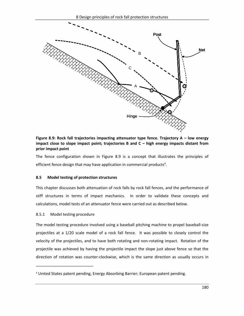
8 Design principles of rock fall protection structures
180
Post
Net
A
B
C
Hinge
Post
Net
A
B
C
Post
Net
Post
Net
A
B
C
Hinge
Figure 8.9: Rock fall trajectories impacting attenuator type fence. Trajectory A – low energy impact close to slope impact point; trajectories B and C – high energy impacts distant from prior impact point
The fence configuration shown in Figure 8.9 is a concept that illustrates the principles of
efficient fence design that may have application in commercial products4.
8.5 Model testing of protection structures
This chapter discusses both attenuation of rock falls by rock fall fences, and the performance of
stiff structures in terms of impact mechanics. In order to validate these concepts and
calculations, model tests of an attenuator fence were carried out as described below.
8.5.1 Model testing procedure
The model testing procedure involved using a baseball pitching machine to propel baseball-size
projectiles at a 1/20 scale model of a rock fall fence. It was possible to closely control the
velocity of the projectiles, and to have both rotating and non-rotating impact. Rotation of the
projectile was achieved by having the projectile impact the slope just above fence so that the
direction of rotation was counter-clockwise, which is the same direction as usually occurs in
4 United States patent pending, Energy Absorbing Barrier; European patent pending.
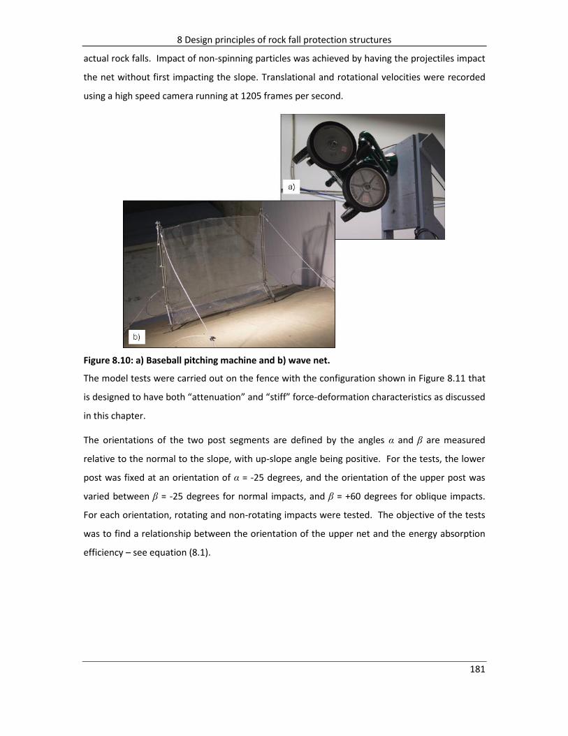
8 Design principles of rock fall protection structures
181
actual rock falls. Impact of non-spinning particles was achieved by having the projectiles impact
the net without first impacting the slope. Translational and rotational velocities were recorded
using a high speed camera running at 1205 frames per second.
Figure 8.10: a) Baseball pitching machine and b) wave net.
The model tests were carried out on the fence with the configuration shown in Figure 8.11 that
is designed to have both “attenuation” and “stiff” force-deformation characteristics as discussed
in this chapter.
The orientations of the two post segments are defined by the angles α and β are measured
relative to the normal to the slope, with up-slope angle being positive. For the tests, the lower
post was fixed at an orientation of α = -25 degrees, and the orientation of the upper post was
varied between β = -25 degrees for normal impacts, and β = +60 degrees for oblique impacts.
For each orientation, rotating and non-rotating impacts were tested. The objective of the tests
was to find a relationship between the orientation of the upper net and the energy absorption
efficiency – see equation (8.1).

8 Design principles of rock fall protection structures
182
vi
PostNet
α = -25˚
β = +40˚ +ωi
ψs = 30˚
Figure 8.11: Configuration of rock fall fence used in model tests. Orientations of hinged posts are defined by angles α and β, measured relative to the normal to the slope
8.5.2 Model test parameters
The baseball pitching machine allowed the translational velocity of the projectile, as well as its
rotational velocity to be controlled, with values selected to achieve impacts with high enough
energy to significantly deflect the net. The translational velocities varied between 7 and 27 m ·
s-1 (25 to 90 ft · s-1), and the rotation was counter-clockwise for the model shown in Figure 8.12.
The projectile was a dense rubber ball with a dimpled surface, a diameter of 75 mm (3 in) and a
mass of 140 gram (0.3 lb). For a sphere, the rotation parameters are: radius of gyration, k =
(2/5)0.5 · r = 0.024 m and moment of inertia, I = m · k2 = 7.9E-5 kg · m2.
8.5.3 Results of model tests
For the model tests, the image analysis software, ProAnalyst© (Xcitex, 2008), was used to find
the impact (initial) velocities, Vi, ωi and final (restitution) velocities, Vf, ωf from which the initial
and final total energies could be calculated. Figure 8.12 shows a typical result of an oblique
angle impact between the projectile and the fence inclined up-slope, and the reduction in
velocity that occurs during impact. The image shows the redirection by the net of the body,

8 Design principles of rock fall protection structures
183
which “rolls” down the net during impact; contact duration is 0.0506 seconds (61 frames).
During this contact duration the velocity decreases from Vi = 14.6 m · s-1 (48 ft · s-1) at the point
of impact to a minimum velocity of 8.3 m · s-1 (27 ft · s-1) between frames #90 to #99,
approximately 0.03 seconds after impact. After this time, the velocity increases slightly to Vf =
9.41 m · s-1 (31 ft · s-1) as projectile starts to rebound off the net. These velocity changes
illustrate “attenuation” type behavior of the fence.
Figure 8.12: Path of deflected projectile after impact with net oriented up-slope (β = +60 degrees). Approximate velocities at ten frame intervals (0.0083 s) during impact shown
The changes in velocity were then used to find a relationship between the fence orientation
defined by the angle β and the energy efficiency Ee (see equation (8.1)), where the energy
efficiency increases when more of the impact energy retained by the moving projectile and less
is absorbed by the net. For a projectile that is stopped by the net and all the impact energy is
absorbed, the energy efficiency is zero.

8 Design principles of rock fall protection structures
184
Figure 8.13 shows the relationship between the angle β and the energy efficiency. That is, when
normal impact occurs (β = 0), all the energy is absorbed and Ee = 0. For a non-rotating body, the
energy efficiency increases as the upper net is inclined further up-slope (angle β increases)
showing the effect of the body being re-directed due to the oblique impact angle. When β = 60
degrees, only about 50 per cent of the impact energy is absorbed.
Figure 8.13: Relationship between energy efficiency and angle β of upper net, for a non-rotating body
The test results also provided information on the changes in velocity and impulse over the
duration of the impact. For example, the relationship between the velocity and duration that
the body is in contact with the net is shown in Figure 8.14 for a variety of tests in which the β
angle varied from 0 to 60 degrees. The velocity decreases during contact from an initial value of
about 15 m·s-1 to a minimum value of about 7 m·s-1 before increasing slightly as the body starts
to rebound off the net. At no time does the velocity approach zero indicating that only a portion
of the impact energy is absorbed by the net.

8 Design principles of rock fall protection structures
185
Figure 8.14: Relationship between the duration of impact and change in velocity during impact
The velocity, V data shown in Figure 8.15 can be expressed as an impulse, (p = m · V) where m is
the mass of the body. For the baseball-size body used in the tests with a mass of 0.14 kg (0.3 lb),
impulse values were calculated for the corresponding velocities measured during the impact.
Figure 8.15 shows the relationship between the duration of the impact and the percentage of
the impact impulse that is absorbed by the fence during impact. That is, the impulse begins to
be absorbed very soon after impact, and increases steadily during the impact.
The form of the actual [time – impulse] relationship shown in Figure 8.15 can be compared with
the theoretical relationship between [time – force] shown in Figure 8.6 where the behavior of
rigid, flexible and stiff structures are compared. It is apparent that the fence configuration used
for the model tests has produced a stiff structure that absorbs energy throughout the impact,
thus minimizing the induced force.

8 Design principles of rock fall protection structures
186
Figure 8.15: Relationship between duration of impact and the amount of impulse that is absorbed by the fence; compare with Figure 8.7 for stiff structures
This chapter has examined the theory of designing efficient protection structures that redirect
(attenuate) rather than stop rock falls. This concept has been used in the construction of
hanging net-type fences as shown in Figure 8.4. The author has been involved with the design
and construction of about 25 hanging nets that have been impacted by many hundreds of rock
falls, almost all of which have caused no significant damage to the fence. This performance,
together with theory and model tests, would indicate that attenuator-type structures are
effective in containing rock falls.

9 Conclusions
187 187
9 Conclusions and On-going Research
The research that I have conducted between 2009 and 2013 has been a very rewarding
experience in terms of the intellectual challenge of applying impact mechanics theory to rock
falls, and developing equations defining velocity and energy changes during rock fall impacts. I
started this research with wide experience of rock fall events, and practical knowledge of the
design, construction and performance of protection structures, but little knowledge of the
theoretical aspects of impact behavior and how protection structures function in absorbing
impact energy. My research has provided me with this valuable theoretical knowledge.
I consider that my research over the last five years is a phase in my on-going work to improve
the design and function of rock fall protection structures, and provide better safety for the
public from these hazards.
This chapter summarizes the conclusions that I have developed on rock fall behavior, and the
work that I plan to carry out in the future.
9.1 Conclusions
The three main conclusions that I have drawn from my research are discussed below.
9.1.1 Case studies of rock fall events and testing sites
Because it is difficult to accurately simulate rock falls using mathematical models, it is important
to have documented case studies that can be used to calibrate simulation programs. The five
case studies provide reliable data on rock falls for a wide range of topographic and geologic
conditions that I believe will be good calibration tools. In fact, as of November 2013, the data
are being used to calibrate a modeling program that is under development.
I have a number of other case studies in my files that I hope will be useful to interested
researchers, in addition to those described in this thesis.
One of the interesting findings from examining the case studies was that the normal coefficient
of restitution, eN can be greater than 1 for shallow impact angles, θi (θi < ~20 degrees) and that a
power curve defines the relationship between eN and θi. Furthermore, the normal coefficient of
restitution is not a function of the slope material on which the rock falls impact. That is, it was
found that one of the lowest values for eN (0.18) was for a rock dropped on to a horizontal
concrete surface, while eN values greater than 1 occurred for shallow impacts (θi ≈ 20 degrees)

9 Conclusions
188
on the relatively soft soil/gravel colluvium at Tornado Mountain. This apparent paradox can be
explained by impact mechanics theory for impact of rotating, non-spherical bodies (see Section
9.1.2 below).
Also, it is important to note that eN > 1 does not mean that energy is being created during
impact. Impact mechanics analysis separates the normal velocities and energy changes due to
inelastic compression and hysteresis of the slope materials, from the tangential velocity and
energy changes due to friction at the contact surface. Therefore, while energy may be gained in
the normal direction, energy will always be lost in the tangential direction, and a net energy loss
will occur for the impact.
The implication of this research finding is as follows. The existing rock fall modelling programs
relate eN and eT values to the slope material and assume that these are material properties.
However, the research shows that it would be more appropriate to use a specific eN value for
each impact related to the impact angle θi, with the value of θi determined from the geometrics
of the impact.
Values of eT to use in rock fall modelling are always less than 1 due to friction acting on the
contact surface, and may be related to the roughness of the surface. The field data shows that
eT values lie between about 0.3 and 0.9, and that eT is independent of the slope material and the
body shape. The lowest value for et was 0.24 for the relatively smooth asphalt surface.
9.1.2 Impact mechanics theory
I found that my application of Dr. Stronge’s impact mechanics to rock falls has been most useful
in developing a detailed understanding of the impact behavior; I believe that this is the first
application of Dr. Stronge’s methods to rock falls. That is, the use of the normal impulse, pN as
an independent variable that is tracked during impact, shows that a linear relationship exists
between the normal impulse and the relative velocity, v. This linear relationship between pN
and v can be plotted on a [pN – v] diagram that shows the normal, tangential and rotational
velocity components at any stage of the impact. Equations for velocity and angle changes
during impact were developed for collinear impact of a rough, rotating sphere.
A further function of [pN – v] diagrams is that inelastic compression and rebound phases of
impact are separated so that the corresponding energy changes can be calculated, in both the
normal and tangential directions.

9 Conclusions
189
The finding that the normal coefficient of restitution is related to the impact angle, and can be
greater than 1, only occurs for eccentric impact where a non-spherical, rough rotating body
impacts the slope at a shallow angle (θi < ~20 degrees) . These impact conditions can be
examined using [pN – v] diagrams where the changes in the normal and shear components of
velocity during impact are represented asstraight lines. The slope of the line depends on the
mass and shape of the impacting body and its rotational velocity, while the intercept of the line
depends on the normal component of impact velocity. Typical [pN – v] plots show that values of
eN increase as the impact angle θi decreases, i.e., becomes flatter, and that eN can have values
greater than 1.
This theoretical relationship between eN and θi with eN being greater than 1 for shallow impacts,
supports the findings of the field studies.
9.1.3 Performance of rock fall protection structures
Rock fall fences and nets can provide protection against rock falls by either stopping or
redirecting rock falls. If a rock fall is stopped by the net, then all the impact energy is absorbed
by the net. However, if the rock is redirected by the net so that its velocity is only reduced, then
a portion of the impact energy is absorbed with the remainder of the energy being retained in
the moving rock. The lower velocity falls can then be contained in a less expensive containment
structures such as a ditch or low energy capacity barrier.
Furthermore, if a “stiff” structure is used in which the impact energy is absorbed uniformly
during impact, compared to highly “flexible” nets that only absorb energy at large deflections,
then impact forces induced in the net are minimized. This behavior of stiff nets and fences that
redirect rock falls is demonstrated both from the theory of impact mechanics and scale model
tests. The tests involved using a baseball pitching machine to project baseballs at the net and a
high speed camera to record the changes in translational and rotational velocities during impact.
The impact calculations and model test results provide consistent results.
Structures that redirect and reduce the velocity of falls, rather than stop falls, are termed
“attenuators”. Various net configurations that achieve this function are hanging nets, fences
that are inclined up-slope (“Wave nets”) and canopies.
The implication of this performance of stiff, attenuator protection structures is that it should be
possible to use lighter, smaller structures to contain rock falls. That is, these structures will be

9 Conclusions
190
less expensive than structures currently used so that more nets can be installed to provide
greater protection for the public in rock fall hazard environments.
9.2 Future research work
As stated above, my research over the past five years is part of my on-going study of rock fall
behavior. It is my intention to continue with this work in the future that I plan will involve the
following activities.
9.2.1 Additional case studies
Over the course of my engineering work I expect that I will study other rock fall events and that
these will be added to my compendium of case studies. If this work provides useful results, I
would make them available to others working in this field.
It will be most valuable to collect additional field data on the relationship between the normal
coefficient of restitution and the impact angle. These data will help to refine the relationship
between these two parameters, and may show how that other characteristics of rock fall
impacts influence eN, in addition to the impact angle.
9.2.2 Impact mechanics
The impact model described in this thesis applies to bodies of any shape defined by their radius,
r and radius of gyration, k. However, the equations developed in this thesis for changes in
velocity and energy during impact apply to only collinear impact for translating and rotating,
rough spheres. It is my intention to develop equations for velocity and energy changes that
apply to eccentric impact for any body shape. These equations will then be used to compare
theoretical behavior with the case study results where eccentric impacts of non-spherical bodies
occur.
Another valuable investigation would be to analyze high speed photography of actual rock fall
impacts to measure changes in relative velocity and normal impulse during impact. These
results could then be plotted on [pN – v] diagrams to see how closely actual impact behavior
matches impact mechanics theory. This information would be used to make appropriate
modifications to the theoretical equations in order to develop equations that would reliably map
actual velocity and energy changes during impact.

9 Conclusions
191
It is noted in this thesis that the actual velocity and energy changes during impact are greater
than those calculated using theoretical impact mechanics, probably because the theory does not
fully account for the plastic conditions that occur in actual impacts.
9.2.3 Protection structures
The model tests of rock fall fences carried out with the baseball pitching machine showed that
stiff structures that redirect falls are effective in efficiently containing rock falls. It is now
planned to carry out full scale testing in a local quarry. The tests will involve various
configurations of both wave nets and hanging nets, with concrete blocks of various sizes used as
the projectile; the velocity and impact energy will be controlled by varying the fall height. Data
will be collected using a three-dimensional accelerometer in the concrete block, load cells in the
guy cables and a high speed camera. The information will be recorded in a data acquisition
system operating at 2 kHz.
It is intended that the field tests, together with theoretical studies of impact mechanics, will be
used to develop improved rock fall protection nets and fences. Specifically, the tests will
investigate the relationships between changes in velocity and energy during impact, and the
configuration of the net, such as the incidence angle and the stiffness of the net. One of the
potential benefits of stiff nets compared to the present highly flexible nets will be that less
deformation will occur with a stiff net. This will allow nets to be located closer to the structure
being protected which will reduce installation and maintenance costs.
192 192
References
Ashayer, P. (2007). Application of rigid body impact mechanics and discrete element modeling to rockfall simulation. Ph.D. thesis, University of Toronto, Grad. Dept. of Civil Engineering.
Asteriou, H., Saroglou, G. and Tsiambaos, T. (2012). Geotechnical and kinematic parameters affecting the coefficient of restitution for rock fall analysis. Int. J. Rock Mechanics and Mining Sciences, 54, pp 103 – 113, September.
Beladjine, D., Ammi, M., Oger, L. and Valance, A. (2007). Collision process between an incident bead and a three-dimensional granular packing. Physical Review E, 75: 1-12.
Benjamin, J. R. and Cornell, A. C. (1979). Probability, Statistics and Decision for Civil Engineers. McGraw-Hill, New York.
Bichler, A. and Stelzer, G. (2012). A fresh approach to the hybrid/ attenuator rockfall fence. Proc. 11th Int. Symp. on Landslides (ISL) and the 2nd North American Symp. on Landslides, June 2-8, Banff, Alberta, Canada.
Brunet, G. and Giacchetti, G. (2012). Design software for secured drapery. Proc. 63rd Highway Geology Symp., Redding, CA.
Bugnion, L., Wendeler, C. and Shevlin, T. (2012). Impact pressure measurements in shallow landslides for flexible barrier design. Proc. of the 11th Int. Symp. on Landslides (ISL) and the 2nd North American Symp. on Landslides, June 2-8, 2012, Banff, Alberta, Canada
Bunce, C. M., Cruden, D. M. and Morgenstern, N. R. (1997). Assessment of the hazard from rock fall on a highway. Canadian Geotech. J., Vol. 34, 344-56.
Buzzi, O., Giacomini, A. and Spadari, M. (2012). Laboratory investigation of high values of restitution coefficients. J. Rock Mech. Rock Eng., 43: 35-43.
California Polytechnical State University (1996). Response of the Geobrugg cable net system to debris flow loading. Department of Civil and Environmental Engineering, San Luis Obispo, CA, pp 3, 35, 59.
Canadian Geotechnical Society (2006). Canadian Foundation Engineering Design Manual, 4th Edition. BiTech Publishing, Richmond, British Columbia, 488 pages.
Chau, K. T., Wong, R. H. C., Liu, J. and Lee, C. F. (2003). Rockfall hazard analysis for Hong Kong based on rockfall inventory. Rock Mech Rock Eng, 36(5):383 - 408.
Chau, K. T., Wong, R. H. C. and Wu, J. J. (2002). Coefficient of restitution and rotational motions of rock fall impacts. Int. J. Rock Mech. & Mining Sciences, 39:69-77.
Chen, G., Zheng, L., Zhang, Y. and Wu, J. (2013). Numerical Simulation in Rockfall Analysis: A Close Comparison of 2-D and 3-D DDA. Rock Mechanics and Rock Engineering, 46(3), 527-541.
Dellow, G., Yetton, M., Archibald, G., Barrell, D.J.A., Bell, D., Bruce, Z., Campbell, A., Davies, T., De Pascale, G., Easton, M., Forsyth, P.J., Gibbons, C., Glassey, P., Grant, H., Green, R., Hancox, G., Jongens, R., Kingsbury, P., Kupec, J., MacFarlane, D., McDowell, B., McKelvey, B., McCahon, I., McPherson, I., Molloy, J., Muirson, J., O'Halloran, M., Perrin, N., Price, C., Read, S., Traylen, N., Van Dissen, R., Villeneuve, M. and Walsh, I. (2011) Landslides Caused by the 22 February 2011 Christchurch Earthquake and Management of Landslide Risk in the

193
Immediate Aftermath. Bulletin of the New Zealand Society for Earthquake Engineering 44(4): 227-238.
Dijkstra, T. A., Chandler, J., Wackrow, R., Meng, X. M., Ma, D. T., Gibson, A., Whitworth, M., Foster, C., Lee, K., Hobbs, P. R. N., Reeves, H. J. and Wasowski, J. (2012). Geomorphic controls and debris flows - the 2010 Zhouqu disaster, China. Proceedings of the 11th International Symposium on Landslides (ISL) and the 2nd North American Symposium on Landslides, June 2-8, 2012, Banff, Alberta, Canada.
Dorren, L. K. A. and Berger, F. (2012). Integrating forests in the analysis and management of rock fall risks: experience from research and practice in the Alps. Proc. 11th Int. Conf. and 2nd North American Symp. on Landslides and Engineered Slopes. Banff, Canada, June 2012, p. 117-127.
Dorren, L. K. A., Berger, F. and Putters, U. S. (2006). Real size experiments and 3-D simulation of rock fall on forested and non-forested slopes. Natural Hazards and Earth Science Systems, 6: 145-53.
Dorren, L. K. A., and Berger, F. (2005). Stem breakage of trees and energy dissipation during rock fall events. Tree Physiology, 26:63-71.
European Organisation for Technical Approvals (February 1, 2008). ETAG 27, Guideline for European Technical Approval of Falling Rock Protection Kits. EOTA. Retrieved on May 22, 2013, from http://www.eota.be/pages/home/
Geobrugg (2012). RUVOLUM Online Tool, Version 2012 software. Geobrugg AG, Switzerland. Retrieved on May 22, 2013, from http://applications.geobrugg.com/
Geobrugg (2010). Product literature - TECCO damping modules for rock fall protection galleries. Romanshorn, Switzerland.
Giacchetti, G., Grimod, A. and Cheer, D. (2011). Soil nailing with flexible facing: design and experience. Proc. Second World Landslide Forum, Rome, October.
Giacchetti, G. and Zotti. I. M. (2012). Design Approach for Rockfall Barriers. Geotechnical XI National Congress in Costa Rico (August 9 and 10). San Jose, Costa Rica, 2012.
Giacomini, A., Thoeni, K., Lambert, C., Booth, S. and Sloan, S. W. (2012). Experimental study on rockfall drapery systems for open pit highwalls. Int. J. of Rock Mechanics and Mining Sciences 56(0): 171-181.
Giacomini, A., Spadari, M., Buzzi, O., Fityus, S. G. and Giani, G. P. (2010). Rockfall motion characteristics on natural slopes in eastern Australia. Eurock 2010, Lausanne, Switerland, 15 to 17, June.
Goldsmith, W. (1960). Impact – Theory and Physical Behaviour of Colliding Solids (2001 edition). Dover Publications, New York, 379 pages.
Grimod, A. and Giacchetti, G. (2011). Protection from high energy impacts using reinforced earth embankments: design and experience. Proc. 2nd World Landslide Forum, Rome, October.
Gutenberg, B. and Richter, C. F. (1954). Seismicity of the Earth, 2nd. Ed. Princeton University Press, Princeton, NJ.
Hambleton, J. P., Buzzi, O., Giacomini, A., Spadari, M. and Sloan, S. W. (2013). Perforation of Flexible Rockfall Barriers by Normal Block Impact. Rock Mechanics and Rock Engineering 46(3): 515-526.

194
Harp, E. L., Jibson, R. W., Kayen, R. E., Keefer, D. K., Sherrod, B. L., Carver, G. A., Collins, B. D., Moss, R. E. S. and Sitar, N. (2003). Landslides and liquefaction triggered by the M7.9 Denali Fault earthquake of 3 November, 2002. GSA Today, August 2003, 10 pages.
Harp, E. L. and Jibson, R. W. (1995). Inventory of landslides triggered by the 1994 Northridge, California earthquake. Dept. of the Interior, USGS, Open file Report 95-213, 17 pages.
Harp, E. L. and Wilson, R. C. (1995). Shaking intensity thresholds for rock falls and slides: evidence from 1987 Whittier Narrows and Superstition Hills earthquakes strong motion records. Bull. Seismological Soc. Am., 85(6), 1739-57.
Harr, M. E. (1977). Mechanics of Particulate Matter - a Probabilistic Approach." McGraw-Hill, New York: 543 pages.
Hungr, O. and Evans, S. G. (1988). Engineering evaluation of fragmental rock fall hazards. Proc. 5th Inter. Symp. on Landslides, Lausanne, Switzerland, July, 685-90.
Hungr, O., Evans, S. G. and Hazzard, J. (1999). Magnitude and frequency of rock falls and rock slides along the main transportation corridors on southwestern British Columbia. Can. Geotech. J.,36: 224-238.
Jacquemoud, J. (1999). Swiss Guideline for the design of rock fall protection galleries: background, safety concept and case histories. Proc. Joint Japan-Swiss Seminar on Impact Load by RockFalls and Design of Protection Measures. Kanazawa, Japan, October, 161 pages.
Japan Road Association (2000). Rock Fall Control Manual (in Japanese). 422 pages.
Jibson, R. W. and Harp, E. L. (1995). Inventory of Landslides Triggered by the 1984 Northridge, California Earthquake. U. S. Dept. of the Interior, USGS, Open file 95-213, 17 pp.
Jones, C. L., Higgins, J. D. and Andrew, R. D. (2000). Colorado Rockfall Simulation Program, version 4.0 (CRSP). CO Dept. of Transportation, Denver, CO, Report no. CDOT-STMB-CGS-99-1, 127 pages.
Keefer, D. K. (1992). The susceptibility of rock slopes to earthquake-induced failure. Proc. 35th Annual Meeting of the Assoc. of Eng. Geologists, (ed. Martin L. Stout), Long Beach, CA, 529-38.
Kirsten, H. A. D. (1982). Design and construction of the Konwyn’s Pass rock fall shelter. Civ. Engr. S. Afr, 24(9), 477-92.
Kobayashi, Y., Harp, E. L. and Kagawa, T. (1990). Simulation of rock falls triggered by earthquakes. J. Rock Mech. Rock Eng., 23(1):1-20.
Komura, T., Muranishi, T., Nisizawa, K. and Masuya, H. (2001). Study on parameters concerning impact of falling rock on field slopes and rock fall simulation method. Proc. 4th Asia-Pacific Conf. on Shock and Impact Loads on Structures, 345-352.
Labouise, V., Descoeudres, F. and Montani, S. (1996). Experimental study of rock sheds impacted by rock blocks. Struct. Eng. Int., Vol. 3, 171-6.
Maccaferri S.p.A. (2012). Slope mesh design software, BIOS and Mac.Ro1. Maccaferri S.p.A., Bologna, Italy.
Maccaferri S.p.A, Bologna, Italy (2012). Rockfall and Debris Flow Protection Embankments. Product literature, www.maccaferri.ca.

195
Maggs, Micheal (2007, October 8). Bouncing ball strobe edit, in Wikimedia Commons. Retrieved May 22, 2013, from https://en.wikipedia.org/wiki/File:Bouncing_ball_strobe_edit.jpg
Mamaghani, I. H. P, Yoshida, H. and Obata, Y. (1999). Reinforced expanded polystyrene Styrofoam covering rock sheds under impact of falling rocks. Joint Japan-Swiss scientific seminar on impact loads by rock falls and design of protective structures, Kanazawa, Japan, Oct., 79-89.
Masuya, H., Amanuma, K., Nishikawa, Y. and Tsuji, T. (2009). Basic rock fall simulation with consideration of vegetation and application of protection measures. Nat. Hazards and Earth Systems Sciences, 9:1835-43.
Masuya, H., Ihara, T., Onda, S. and Kamijo, A. (2001). Experimental study on some parameters for simulation of rock fall on slope. Proc. 4th Asia-Pacific Conf. on Shock and Impact Loads on Structures, 63-69.
McCauley, M. L.,Works, B. W. and Naramore, S. A. (1985). Rock fall mitigation. Report FHWA/CA/TL-85/12. FHWA, U.S. Department of Transportation.
National Cooperative Highway Research Program (NCHRP) (1999). Geotechnical related development of load and resistence factor design (LRFD). Synthesis of Highway Practice (276), TRB, Washington, D. C., 69 pages.
Newmark, N. M. (1965). Effects of earthquakes on dams and enbankments. Geotechnique, 15(2), 139-160.
Newton, I. (1687). Philosophiae Naturalis Principia Mathematica. Cambridge, U.K.: Cambridge University Press.
Nocilla, N., Evangelista, A. and di Santolo, A. S. (2009). Fragmentation of rock falls: two Italian case studies of hard and soft rocks. Rock Mech. Rock Eng. 42:815-833.
Nishikawa, Y., Masuya, H. and Moriguti, Y (2012). Three dimensional simulation of rock fall motion with consideration of roughness of the slope surface. Trans. Japan Soc. for Computational Engineering and Science, 2012, 20120003.
Palisade Corporation (2012). Computer program @RISK, version 5.0. Palisade Corporation, Ithaca, New York, USA. www.palisade.com
Patton, F. D. (1974). Multiple modes of shear failure in rock. Proc. 1st. Int. Cong. on Rock Mechanics, Lisbon, 1, 509-13.
Peckover, F. L. (1975). Treatment of rock falls on railway lines. American Railway Engineering Association, Bulletin 653, Washington, D. C., pp. 471-503.
Pfeiffer, T. J. and Bowen, T. D. (1989). Computer simulation of rock falls. Bull. Assoc. Engineering Geologists, Vol XXXVI, No. 1, 135-46.
Pfeiffer, T. J., Higgins, J. D.D. J., Andrew, R. D., Schultz, R. J. and Beck, R. B. (1995). Colorado Rock Fall Simulation Program. Version 3.0, User's Manual. Colorado Department of Transportation.
Pfeiffer, T. J. and Higgins, J. D. (1995). Rockfall hazard analysis using the Colorado Rockfall Simulation Program. TRB, Washington, DC, Transportation Research Record 1288, 117-26.
Pierson, L. A., Davis, S. A., and Van Vickle, R. (1990). The Rock Fall Hazard System, Implementation Manual. Technical Report, #FHWA-OR-EG-90-01, Washington, D. C.

196
Pierson, L. A., Gullixson, C. F. and Chassie, R. G. (2001). Rockfall Catchment Area Design Guide. Research Report SPR-3(032): Oregon Department of Transportation-Research Group, Federal Highway Administration.
Piteau and Associates Ltd. (1980). Slope stability analysis for rockfall problems: the computer rockfall model for simulating rockfall distributions, Part D. Rock Slope Engineering, reference manual FHWA-TS-79-208. FHWA, Department of Transportation, Washington D.C., 62-8.
Poisson, S. D. (1811). Traité de Méchanique. Courier, Paris. (English translation by Rev. H. H. Harte, Longman & Co 1817).
Protec Engineering, Niigata, Japan (2012).MSE embankments for rock fall containment. Technical literature, www.proteng.co.jp.
Raiffa, H. (1968). Decision analysis: introductory lectures on choices under uncertainty. Addison-Wesley, Reading MA, 309 pages.
Ritchie, A. M. (1963). An evaluation of rock fall and its control. Highway Research Record 17, Highway Research Board, NRC, Washington DC, pp. 13-28.
RGHRG (Railway Ground hazard Research Group), 2012. Annual Meeting, Vancouver, Canada, December.
Rochet, L. (1987). Application des modeles numeriques de propagation a l'tude des eboulements rocheux. Bulletin de liaison laboratorires des ponts et chaussees. 150-1, Sept.-Oct..
RocScience (2012). Computer program RocFall 4.0. RocScience Inc., Toronto, Canada.
Schellenberg, K. and Vogel, T. (2009). A dynamic design method for rockfall protection galleries. J. Int. Assoc. Bridge and Structural Eng., SEI Vol. 19(3), 321-6.
Skermer, N. A. (1984). M Creek debris flow disaster. Canadian Geotechnical Conference: Canadian Case Histories, Landslides, Toronto, pp.187-94.
Spadari, M., Giacomini, A., Buzzi, O., Fityus, S. G. and Giani, G. P. (2012). In situ rock fall testing in New South Wales, Australia. Int. J. Rock Mechanics and Mining Sciences, 49, pp 84 – 93.
Stevens, W. D. (1998). RocFall: a tool for probabilistic analysis, design of remedial measures and prediction of rock falls. Thesis for M. App. Sc. degree, University of Toronto, Dept. of Civil Eng., 28 pages.
Stock, G. M., Luco, N., Harp, E. L., Collins, B. D., Reichenbach, P., Frankel, K. L., Matasci, B., Carrea, D., Jaboyedoff, M., Oppikofer, T. (2012). Quantitative rock fall hazard and risk assessment in Yosemite Valley, California, USA. Proc. 11th Int. Conf. and 2nd North American Symp. on Landslides and Engineered Slopes. Banff, Canada, Vol.2, 1119-1125.
Stock, G. M., Sitar, N., Borchers, J. W., Harp, E. L., Snyder, J. B., Collins, B.D., Bales, R.C., Wiezorek, G.F. (2012). Evaluation of hypothesized water-system triggers for rock falls from Glacier Point, Yosemite National Park, California, USA. Proc. 11th Int. Conf. and 2nd North American Symp. on Landslides and Engineered Slopes. Banff, Canada Vol.2, 1165-1171.
Stronge, W. J. (2000). Impact Mechanics. Cambridge University Press, Cambridge, U. K., 280 pages.
Transportation Research Board (TRB) (1996). Landslides, Investigation and Mitigation. National Research Council, Special Report 247, Washington DC, 673 pages.
197
Ushiro, T. and Tsutsui, H. (2001) T. Hideki. Movement of a Rockfall and a Study on Its Prediction. Proceeding of the International Symposium on Geotechnical & Environmental Challenges in Mountainous Terrain. Ehime, Japan, Nov. 2001: 275-285
Ushiro, T., Kusumoto, M., Shinohara, S. and Kinoshita, K. (2006). An experimental study related to rock fall movement meshanism. J. Japan Soc. of Civil Engineers, Series F, 62(2), 377-386 (in Symp. on Geotechnical and Environmental Challenges in Mountainous Terrrain, Kathmandu, Nepal, 366-375.
Vogel, T., Labiouse, V. and Masuya, H. (2009). Rockfall protection as an integral task. Structural Engineering International, SEI Vol. 19(3), 304-12, IABSE, Zurich, Switzerland, www.iabse.org
Watts, C.F., Underwood, S.A., Haneberg, W.C., Rogers, J.D. (2012). Fully rationalized equations for incorporating joint water pressure in rock slope stability analyses at Glacier Point in Yosemite National Park, California. Proc. 11th Int. Conf. and 2nd North American Symp. on Landslides and Engineered Slopes. Banff, Canada, Vol.2, 1173-1178.
Wu, Shie-Shin (1985). Rockfall Evaluation by Computer Simulation, Transportation Research Record 1031, 1-5.
Wyllie, D. C. (1987). Rock slope inventory system. Proc. Federal Highway Administration Rock Fall Mitigation Seminar, FHWA, Region 10, Portland, OR.
Wyllie, D. C. (1999). Foundations on Rock (second edition). E&FN Spon, London, UK, 401 pages.
Wyllie, D. C. and Mah, C. W. (2002). Rock Slope Engineering, fourth edition. Taylor and Francis, London, UK, 422 pages.
Wyllie, D. C. (2006). Risk management of rock fall hazards. Proc. 59th Annual Canadian Geotechnical Conference, Canadian Geotech. Soc., Vancouver, Canada.
Wyllie, D. C., McCammon, N. R. and Brumund, W. F. (1979). Use of risk analysis in planning slope stabilization programs on transportation routes. Transportation Research Board, Research Record 749, Washington D.C..
Xcitex (2008). Proanalyst©, Motion Analysis Software. Xcitex Inc., Cambridge, MA, USA.
Yokoyama, K., Ohira, M. and Yoshida, H. (1993). Impulsive properties due to rock fall on a steel rock shed (in Japanese), J. of Struct. Eng., Vol.39A, 1573-1586.
Yoshida, H., Nomura, T., Wyllie, D. C., & Morris, A. J. (2007). Rock fall sheds - application of Japanese designs in North America. Proc. 1st. North American Landslide Conference, Vail, CO.,AEG Special Publication No. 22., ed. Turner, A. K., Schuster, R. L., 179-196.
Zhang, R. and Rock, A. (2012). Rockfall stimulation using a 3-D discrete element model with engineering validation. Proc. 11th Int. Conf. and 2nd North American Symp. on Landslides and Engineered Slopes. Banff, Canada, Vol.2, 1153-1164.
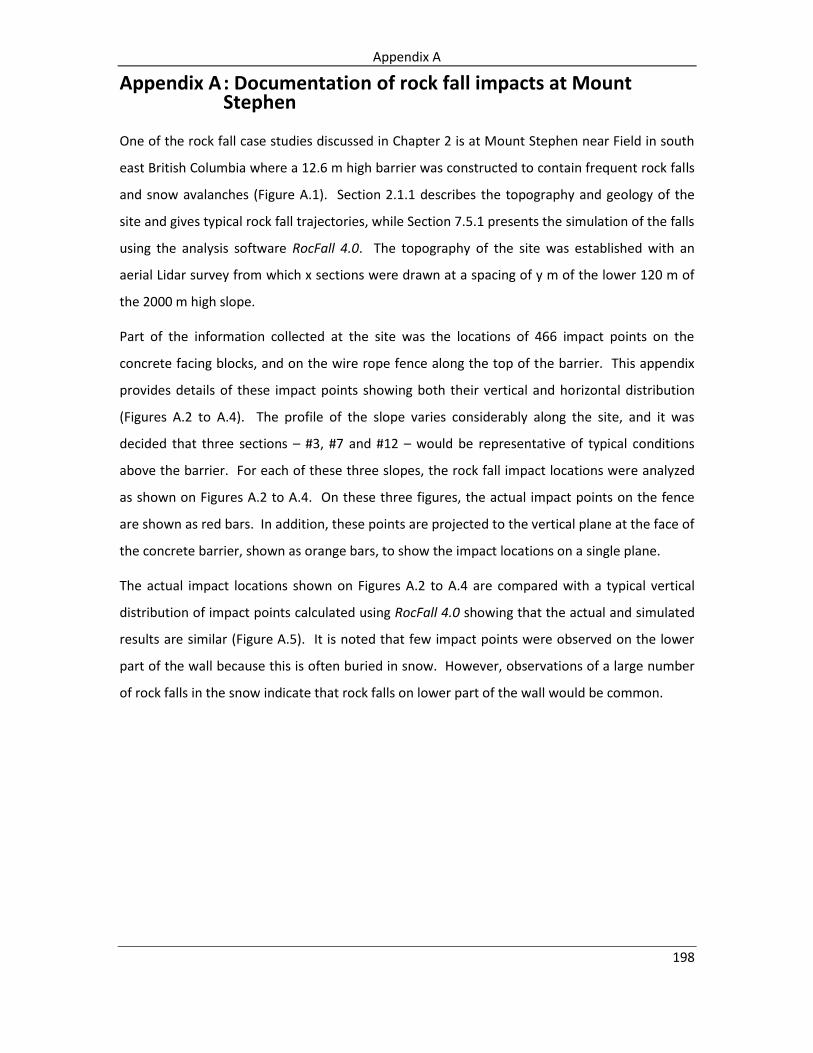
Appendix A
198 198
Appendix A : Documentation of rock fall impacts at Mount Stephen
One of the rock fall case studies discussed in Chapter 2 is at Mount Stephen near Field in south
east British Columbia where a 12.6 m high barrier was constructed to contain frequent rock falls
and snow avalanches (Figure A.1). Section 2.1.1 describes the topography and geology of the
site and gives typical rock fall trajectories, while Section 7.5.1 presents the simulation of the falls
using the analysis software RocFall 4.0. The topography of the site was established with an
aerial Lidar survey from which x sections were drawn at a spacing of y m of the lower 120 m of
the 2000 m high slope.
Part of the information collected at the site was the locations of 466 impact points on the
concrete facing blocks, and on the wire rope fence along the top of the barrier. This appendix
provides details of these impact points showing both their vertical and horizontal distribution
(Figures A.2 to A.4). The profile of the slope varies considerably along the site, and it was
decided that three sections – #3, #7 and #12 – would be representative of typical conditions
above the barrier. For each of these three slopes, the rock fall impact locations were analyzed
as shown on Figures A.2 to A.4. On these three figures, the actual impact points on the fence
are shown as red bars. In addition, these points are projected to the vertical plane at the face of
the concrete barrier, shown as orange bars, to show the impact locations on a single plane.
The actual impact locations shown on Figures A.2 to A.4 are compared with a typical vertical
distribution of impact points calculated using RocFall 4.0 showing that the actual and simulated
results are similar (Figure A.5). It is noted that few impact points were observed on the lower
part of the wall because this is often buried in snow. However, observations of a large number
of rock falls in the snow indicate that rock falls on lower part of the wall would be common.

Appendix A
199
5696300
5696250
5696200
5696150
5696100
5696050
5696000
538650 538700 538750 538800 538850 538900
Lockblock wall and fe
nce
#12
#7
#3
1400
Figure A.1: Plan of Lockblock wall/ fence and slope

Appendix A
200
Lockblock wall
10 blocks high
(6.6 m)
Ringnet Fence
5 m high
Height (m)
Number of Impacts
20 40 60 80
0
1
2
3
4
5
6
7
8
10
11
12
9
13
-1
-2
0
1
2
3
4
5
6
7
8
10
11
12
9
13
-1
-2
Figure A.2: Section #3. a) Cross section view, b) distribution of impact points
b)
a)

Appendix A
201
Lockblock wall
10 blocks high
(6.6 m)
Ringnet Fence
5 m high
Height (m)
Number of Impacts
20 40 60 80
0
1
2
3
4
5
6
7
8
10
11
12
9
13
-1
-2
0
1
2
3
4
5
6
7
8
10
11
12
9
13
-1
-2
Figure A.3: Section #7. a) Cross section view, b) distribution of impact points
a)
b)

Appendix A
202
Lockblock wall
10 blocks high
(6.6 m)
Ringnet Fence
5 m high
Height (m)
Number of Impacts
20 40 60 80
0
1
2
3
4
5
6
7
8
10
11
12
9
13
-1
-2
0
1
2
3
4
5
6
7
8
10
11
12
9
13
-1
-2
Figure A.4: Section #12. a) Cross section view, b) distribution of impact points
b)
a)

Appendix A
203
Figure A.5: Calculated vertical distribution impact points on barrier at Mt. Stephen

Appendix B
204 204
Appendix B: Impact mechanics – normal coefficient of restitution
This appendix shows the derivation of the equations defining the normal coefficient of
restitution in terms of the energy loss during compression and the energy recovery during
restitution phases of impact. This is an expansion of the information contained in Section 4.4 of
the main text.
The principle of separating the compression and restitution phases of impact can be
demonstrated on a normal impulse pN, relative velocity v [pN – v] plot as shown in Figure B.1; v is
the velocity at the center of gravity of the body. On this plot, the normal velocity changes
during impact, starting with a negative value (-viN) at the point of impact, increasing to zero at
the point of maximum compression pc, and finally reaching a positive value (vfN) at the point of
separation. Also, the tangential velocity vT decreases continuously during impact from viT at the
point of impact, to vfT at the point of separation. The change in normal velocity is the result of
plastic deformation of the body and slope during impact, while the change in tangential velocity
is the result of frictional resistance on the contact surface.
+N
vi
-viN
vf
vfT
vfN
viT
Velocity, v
compression restitution
viN
pcN pfN
Normal impulse, pN
viT
vfT
vfN
+T
EcN
EfN -EcN
+N
vi
-viN
vf
vfT
vfN
viT
Velocity, v
compression restitution
viN
pcN pfN
Normal impulse, pN
viT
vfT
vfN
+T
EcN
EfN -EcN
Figure B.1: Relationship between normal impulse pN and changes in tangential and normal velocities vT, vN, and energy during impact The [pN – v] plot on Figure B.1 shows the changes in both the normal (vN) and tangential (vT)
velocity components, and the magnitude of the internal energy of deformation generated
during impact. These changes in velocity, as well as energy, can be quantified in terms of the
coefficient of restitution, e that has normal (N) and tangential (T) components as follows:
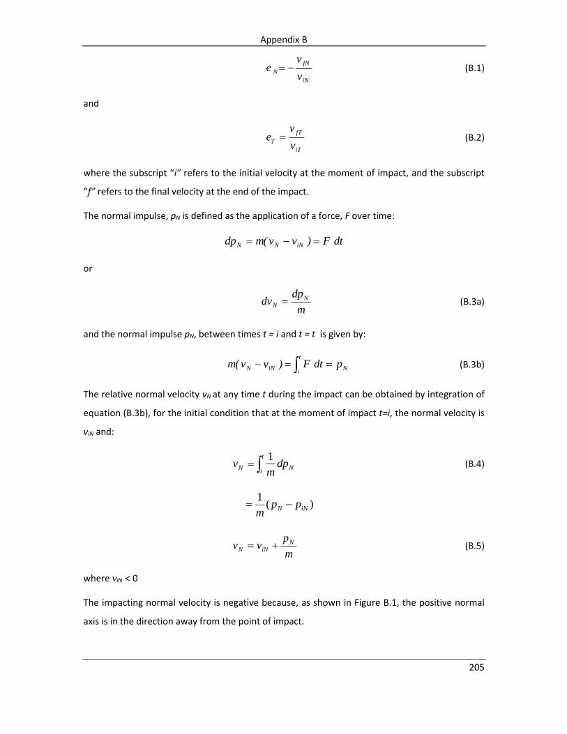
Appendix B
205
iN
fN
Nv
ve (B.1)
and
iT
fT
Tv
ve (B.2)
where the subscript “i” refers to the initial velocity at the moment of impact, and the subscript
“f” refers to the final velocity at the end of the impact.
The normal impulse, pN is defined as the application of a force, F over time:
dtF)vv(mdp iNNN
or
m
dpdv N
N (B.3a)
and the normal impulse pN, between times t = i and t = t is given by:
t
iNiNN pdtF)vv(m (B.3b)
The relative normal velocity vN at any time t during the impact can be obtained by integration of
equation (B.3b), for the initial condition that at the moment of impact t=i, the normal velocity is
viN and:
t
iNN dp
mv
1 (B.4)
)(1
iNN ppm
m
pvv N
iNN (B.5)
where viN < 0
The impacting normal velocity is negative because, as shown in Figure B.1, the positive normal
axis is in the direction away from the point of impact.
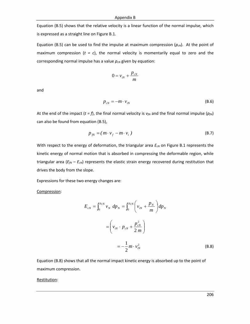
Appendix B
206
Equation (B.5) shows that the relative velocity is a linear function of the normal impulse, which
is expressed as a straight line on Figure B.1.
Equation (B.5) can be used to find the impulse at maximum compression (pcN). At the point of
maximum compression (t = c), the normal velocity is momentarily equal to zero and the
corresponding normal impulse has a value pcN given by equation:
m
pv cN
iN 0
and
iNcN vmp (B.6)
At the end of the impact (t = f), the final normal velocity is vfN and the final normal impulse (pfN)
can also be found from equation (B.5),
)vmvm(p iffN (B.7)
With respect to the energy of deformation, the triangular area EcN on Figure B.1 represents the
kinetic energy of normal motion that is absorbed in compressing the deformable region, while
triangular area (EfN – EcN) represents the elastic strain energy recovered during restitution that
drives the body from the slope.
Expressions for these two energy changes are:
Compression:
N
cNp cNpN
iNNNcN dpm
pvdpvE
0 0
m
ppv cN
cNiN2
2
2
2
1iNvm (B.8)
Equation (B.8) shows that all the normal impact kinetic energy is absorbed up to the point of
maximum compression.
Restitution:

Appendix B
207
fNp
cNp
fNp
cNp
NNiNN
NiNcNfN
m
ppvdp
m
pv)EE(
2
2
m
ppv
m
pv cN
cNiN
fN
iN22
22
22
22
2
iNiN
fN
iN
vmvm
m
pv
where: 222
iNcN vmp
22
22
iNfN
fNiNcNfN
vm
m
ppv)EE(
where: cN
iNiN
p
vmv
2
and 2
21
cN
iN
p
vm
m
2
2
222
22fN
cN
iNfN
cN
iNiNcNfN p
p
vmp
p
vmvm)EE(
2
22
212 cN
fN
cN
fNiN
p
p
p
pvm
2
2 12
1
cN
fN
iNp
pvm (B.9)
where viN < 0.
The expressions in equations (B.8) and (B.9) for the partially irreversible changes in kinetic
energy of normal motion that occur during impact can be used to define the normal coefficient
of restitution, eN as follows:
)(
)()(2
cNN
cNNfNN
NpE
pEpEe
(B.10)

Appendix B
208
This definition of the coefficient of restitution in terms of energy separates the energy loss due
to plastic compression and hysteresis of the contact forces from that due to friction and slip
between the colliding bodies.
The relationships shown in equations (B.8), (B.9) and (B.10) can be combined, for normal impact,
to find the following expression for the normal coefficient of restitution in terms of the normal
impulses at maximum compression (pcN) and at the completion of the impact (pfN):
2
2 1
cN
fN
Np
pe (B.11)
Substitution of the expressions for pcN and pfN in equations (B.6) and (B.7) into equation (B.11),
yields the following expression relating impulse to the coefficient of restitution:
)e(p)e(vmp NcNNiNfN 11 (B.12)
and for the normal coefficient of restitution,
iN
fN
Nv
ve (B.1)
cN
cNfN
Np
ppe
)(
As shown in Figure B.1 and expressed in equation (B.1), the normal coefficient of restitution is
the ratio of final normal velocity to the impact normal velocity, and is also the square root of the
negative ratio of the energy recovered during the restitution phase of the impact to the energy
lost during the compression phase (equation (B.10)).
For rough bodies where slip occurs at the contact point, but the direction of slip is constant, the
two expressions for the coefficient of restitution in equations (B.1) and (B.13) are equivalent.
Appendix C
209 209
Appendix C: Impact mechanics – impact of rough, rotating bodies
This appendix shows the derivation of equations defining the final translational and rotational
velocities due to impact of a rough, rotating body. This is an expansion of the information
contained in Section 4.6.2.
C.1 Equations of relative motion
For a rotating body impacting a slope at an oblique angle, the body will have both translational
v, and angular ω, velocities. The relative velocities at the impact points, expressed as normal and
tangential components, are vN and vT. (Figure C.1). At the contact point, equal and opposite
forces, F, -F are developed that oppose interpenetration of the body into the slope and give
differentials of impulse dp over time dt in the normal and tangential directions that are related
by:
dtFdp (C.1)

Appendix C
210
Figure C.1: Impact mechanics principles for two dimensional (planar) motion a) forces generated at contact point during normal impact; b) impact of rough, rotating sphere on a slope, v = velocity at center of mass, V = relative velocity at impact point
From Newton’s second law (see Section 4.1.2), equations of motion for translation of the centre
of the body with mass m and velocity v, for the normal N and tangential T axes are:
m
dpdV N
N (C.2)
and

Appendix C
211
m
dpdV T
T (C.3)
and for planar rotation of a body with radius r and radius of gyration k:
Tdpkm
rd
2 (C.4)
The relative velocity at the contact point, v, is the difference between the velocity at the center
of mass, V, and the peripheral velocity r·ω. The relative velocity has components vN and vT in the
normal and tangential directions.
Based on these relationships, the planar relative velocity changes are given by:
N
N
N
T
dp
dpm
dv
dv
32
211
(C.5)
from which the tangential and normal components of the velocity changes are
m
dpdpdv NT
T21
(C.6a)
and
m
dpdpdv NT
N32
(C.6b)
where β1, β2 and β3 are inertial coefficients. The definition of the inertial coefficients is shown in
Figure C.2 where a body with mass M impacts the slope with mass M´. A local axis system is set
up at the impact point with the tangential (T) axis parallel to the slope, and the normal (N) axis
normal to the slope with positive away from the slope. The dimensions of the body relative to its
centre of mass and the point of impact are defined by tangential and normal radii, rT and rN and
the radius of gyration kr. If the body is rotating about a fixed z axis, the components of the
moments of inertia for plane motion are defined by the tensor, I´:
22
22
'TTN
NTN
rzmrrm
rrmzrmI (C.7)
that yields three components of the moment of inertia I:
2222;; TTzNTTNNTT rzmIrrmIzrmI (C.8)

Appendix C
212
Inertial coefficient β1 is in relation to the term (rN2 + z2) where z = 1:
2
2
1 1r
N
kM
rm
Inertial coefficient β2 is in relation to the term (m· rT · rN):
22
r
TN
kM
rrm
Inertial coefficient β3 is in relation to the term (z2 + rT 2):
2
2
3 1r
T
kM
rm
where m is the effective mass of the two impacting bodies and is defined as
111 'MMm (C.10)
Since the mass of the slope M' is very large, m = M, the inertial coefficients are reduced to:
2
2
1 1k
rN
22k
rr TN
2
2
3 1k
rT
Equations (C.11) for the inertial coefficients can be applied to any body shape with radius r and
radius of gyration k.
(C.9)
(C.11)

Appendix C
213
+T
+N
+
r
M
M'
rN
rT
N
T
+T
+N
+
r
M
M'
rN
rT
N
T
Figure C.2: Dimensions of rotating, impacting body defining inertial coefficients for plane motion, rotating about z axis through centre of gravity (+)
C.2 Equations of planar motion for impact of rough bodies
For usual rock fall conditions where friction is generated at the impact point, the body may
initially slip from the point of impact until a normal impulse value psN, and then roll during which
time the relative tangential velocity at the contact point vT , is zero (Figure C.3). According to
Coulomb’s law, if the coefficient of friction is μ, then the body will slip at the contact point when
the relationship between the tangential and normal impulses is:
pT = -μ · pN (C.12)
vi
vf
vfT
viT
-ωi-rωi
μpN
r
slipping rolling
viN
pcN pfN
viT
vfT
vfNviS
psN
rωs
-rωi
Normal impulse, pN
Velocity, v
VT
Figure C.3: Changes in rotational (ω) and slip (vs) velocities during impact, and transition from slip to rolling mode when vs = 0; for negative angular velocity: vS = (vT – r·ω)

Appendix C
214
From equation (C.5), the change in relative velocity components during the period of slip in
terms of the normal impulse pN, are:
N
N
N
T
dp
dpm
dv
dv
32
211 (C.13)
and the equations for the change in relative velocity components are given by:
m
dpdv N
T21
(C.14a)
and
m
dpdv N
N32
(C.14b)
Integration of these equations for dvT and dvN for the period t = i to t = vs gives components of
velocity for any normal impulse pN, during the period of slip
NiTT p
mvv 12
(C.15a)
and
NiNN p
mvv 23
(C.15b)
Equations (C.15a, b) show that the relationship between v and pN is linear with the gradient
being proportional to (1/m). The equations also show that tangential velocity decreases
throughout the impact from the impact value viT, while the normal velocity increases from an
initial negative value to a final positive value as it leaves the slope.
At the point of maximum compression during impact, the normal velocity is zero and equation
(C.15b) gives the following expression for the normal impulse pcN
cNiNN p
mvv 230
and
23
iN
cN
vmp (C.16)

Appendix C
215
From Appendix B, equation (B.12), the relationship between the impulses at maximum
compression and the completion of the impact is:
NcNNiNfN epevmp 11 (C.17)
from which it is possible to develop, for a rough, rotating body, an expression for the impulse at
the end of the impact, pfN
23
1
iNN
fN
vmep (C.18)
C.3 Equations of motion for translating and rotating bodies – final velocities
The angular velocity ω can be incorporated into the impact mechanics equations (C.5) to (C.11)
as follows.
For a collinear impact of a sphere with radius r, Figure C.3 shows that rT = 0 and rN = r, and
equations (C.11) are further reduced to:
2
2
1 1k
rN ; β2 = 0; β3 = 1
and equations (C.15a) and b)) for the tangential and normal velocity components simplify to:
NiTT p
mvv 1
(C.19a)
m
pvv N
iNN (C.19b)
For the impacting sphere that is a rigid body, the translational velocity components at the centre
of mass are designated by VT and VN and the differential equations for the changes in velocity
components in terms of the normal impulse are:
NN
NNT dpkm
rd
m
dpdVdp
mdV
2;;
(C.20)
The components of relative velocity at the contact point for collinear impact are:
rVv TT ; NN Vv (C.21)

Appendix C
216
The equations for the relative velocity at the point of impact in terms of the normal impulse are
obtained by integration, for the initial conditions (viT = ViT + r · ωi) and (viN = ViN) as follows:
Tangential velocity:
drdvvv TiTT
NNiTT dp
km
rrdp
mvv
2
NiTT pk
r
mvv
2
2
1
(C.22)
Normal velocity:
NiNN dpm
vv1
m
pvv N
iNN (C.23)
The transition from compression to restitution occurs at the point of maximum compression
when (vcN = 0) and (pcN = -m · viN). Using these relationships, the equations for the tangential and
normal relative velocities can be expressed as dimensionless ratios as follows:
cN
N
iN
iT
iN
T
p
p
k
r
v
v
v
v
2
2
1 (C.24)
and
cN
N
iN
N
p
p
v
v1 (C.25)
When slip stops prior to separation (ps < pf), the relative tangential velocity vsT = 0, and equation
(C.24) can be solved to determine an expression for the impulse ratio at time t = s:
2
2
2
2
11k
rV
rV
kr
vv
p
p
iN
iTiN
iT
cN
sN
(C.26)

Appendix C
217
Furthermore, when sliding halts prior to separation, no changes occur to either the tangential
velocity or the angular velocity from this point until the point of separation, i.e., (vfT = vsT) and
(ωf = ωs).
Expressions for the final tangential and normal velocity components at the centre of mass are:
iN
cN
sNiTfT V
p
pVV
2
2
1k
r
rVV iiT
iT
(C.27)
NiNfN eVV (C.28)
and the final rotational velocity is:
iN
cN
sNif V
p
p
k
rrr
2
2
2
22
1k
r
rV
k
r iiTif
(C.29)
Equations (C.27) and (C.28) for the final tangential and normal velocity components respectively
can then be solved to find the final restitution velocity Vf and angle θf as follows:
22
fNfTf VVV (C.30)
fT
fN
fV
Vanat (C.31)
Figure C.4 shows these equations for the final velocities and angles diagrammatically, in terms of
the three impact parameters: Vi, θi and ωi.
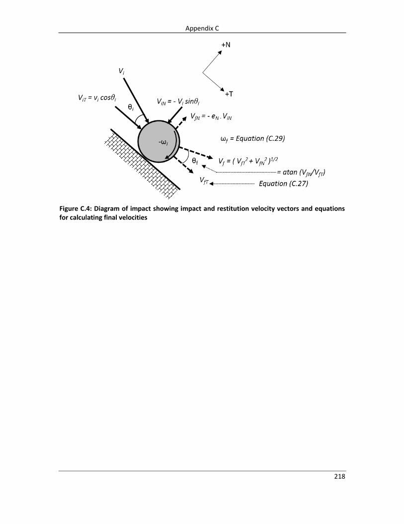
Appendix C
218
Figure C.4: Diagram of impact showing impact and restitution velocity vectors and equations for calculating final velocities

Appendix D
219 219
Appendix D: Energy loss equations
This appendix shows the derivation of equations defining the energy changes that occur during
normal impact of a non-rotating body, and is an expansion of the equations described in Section
6.1 in the main text.
Equations for the energy changes during impact can be developed from the [pN – v] plot
illustrated in Figure D.1 where the impact process is divided into compression and restitution
phases. The energy change during each phase is represented by the areas on the [δ – F] plot or
the [pN – v] plot. The appendix derives the energy changes in terms of the normal impulse pN
and relative velocity v using the linear relationship between these two parameters established in
Appendix B, equation (B.5).
Figure D.1: Energy changes (normal) during compression and restitution phases of impact. a) Forces generated at contact point during normal impact, with energy changes plotted on [force, F – deformation, δ] graph; b) energy changes plotted on [normal impulse, pN – velocity, v] graph
The impact process can be simulated by an infinitesimal deformable particle at the impact point.
During impact, the energy EN generated in the particle by the normal component of the force FN

Appendix D
220
can be calculated from the relationship between the force and the differential normal impulse:
dpN = FN dt = m dv, so that the energy generated from the moment of impact (t = i) up to time t
is:
Np
i NN
t
i NNNdpvdtvFE (D.1)
For the compression phase of the impact up the impulse pcN, the relationships between impulse
and velocity are as follows:
pcN = -m · viN (see equation (B.6))
where viN is negative because it acts towards the slope in the direction of the (–N) axis (see
Figure C.1a).
and
m
pvv N
iNN (see equation (B.5))
Therefore, the energy lost during the compression phase of the impact is given by:
cNp
iNNcNN dpv)p(E
cNp
NN
iN dpm
pv
0
m
ppv cN
cNiN
2
2
2
2
1iNvm (D.2)
where viN is the normal impact velocity and m is the mass of the body.
Equation (D.2) shows that all the normal impact kinetic energy is lost (EN(pcN) is negative) up to
the point of maximum compression, δc when the normal velocity is reduced to zero (vN = 0).
A similar approach can be used to find the energy recovered during the restitution phase of the
impact, (EN(pf) – EN(pc)) between maximum compression (pcN) and the end of the impact (pfN):
N
fNp
cNp
NiNcNNfNN dp
m
pvpEpE

Appendix D
221
m
ppv
m
ppv cN
cNiN
fN
fNiN22
22
22
12
cN
fNiN
p
pvm
The energy recovered during restitution is termed the elastic strain energy. A complete
derivation of equation (D.3) is given in Appendix B, equation (B.9).
Alternatively, the elastic strain energy can be calculated from the area of the restitution triangle
between impulse values pcN and pfN on Figure C.1b as follows:
fNcNfNcNNfNN vpppEpE 2
1
m
pv
p
pp
fN
iN
cN
fN
cN 12
1
cN
iNfN
iN
cN
fNiN
p
vpv
p
pvm1
2
cN
fN
cN
fNiN
p
p
p
pvm11
2
2
22
12
cN
fNiN
p
pvm (D.3)
Equations (D.2) and (D.3) together define the net energy loss during normal impacts as;
EN(net) = [ energy lost in compression ] + [ energy gained in restitution ]
cNNfNNfNN pEpEpE
222
122
cN
fNiNiN
p
pvmvm
22
112 cN
fNiN
p
pvm (D.4)

Appendix D
222
Equation (B.12) defines the relationship between normal impulses pfN, pcN and the normal
coefficient of restitution eN as:
NcNNiNfN epevmp 11 (D.5)
and
N
cN
fNe
p
p 1
and
2
2 1
cN
fN
Np
pe
Substitution of equation of (D.5) into equation (D.4) gives the following expression for the net
energy loss during normal impact:
22 12
1NiNN evmnetE (D.6)
In the development of equation (D.6) for normal impact, the value of eN is always less than 1
because it is defined by the energy losses for a spherical body.

Appendix E
223 223
Appendix E: Conversion factors
Imperial Unit SI Unit SI Unit Symbol Conversion Factor
(Imperial to SI)
Conversion Factor
(SI to Imperial)
Length
Mile kilometer km 1 mile = 1.609 km 1 km = 0.6214 mile
Foot Meter m 1 ft = 0.3048 m 1 m = 3.2808 ft
millimeter mm 1 ft = 304.80 mm 1 mm = 0.003 281 ft
Inch millimeter mm 1 in = 25.40 mm 1 mm = 0.039 37 in
Area
Square mile square kilometer km2 1 mile2 = 2.590 km2 1 km2 = 0.3861 mile2
hectare ha 1 mile2 = 259.0 ha 1 ha = 0.003 861 mile2
Acre hectare ha 1 acre = 0.4047 ha 1 ha = 2.4710 acre
square meter m2 1 acre = 4047 m2 1 m2 = 0.000 247 1 acre
Square foot square meter m2 1 ft2 = 0.092 90 m2 1 m2 = 10.7639 ft2
Square inch square millimeter mm2 1 in2 = 645.2 mm2 1 mm2 = 0.001 550 in2
Volume
Cubic yard cubic meter m3 1 yd3 = 0.7646 m3 1 m3 = 1.3080 yd3
Cubic foot cubic meter m3 1 ft3 = 0.028 32 m3 1 m3 = 35.3147 ft3
liter l 1 ft3 = 28.32 l 1 liter = 0.035 31 ft3
Cubic inch cubic millimeter mm3 1 in3 = 16 387 mm3 1 mm3 = 61.024 x 10⁻⁶ in3
cubic centimeter cm3 1 in3 = 16.387 cm3 1 cm3 = 0.061 02 in3
liter 1 in3 = 0.016 39 l 1 liter = 61.02 in3
Imperial gallon cubic meter m3 1 gal = 0.004 55 m3 1 m3 = 220.0 gal
liter l 1 gal = 4.546 l 1 liter = 0.220 gal
Pint liter l 1 pt = 0.568 l 1 liter = 1.7598 pt
US gallon cubic meter m3 1 US gal = 0.0038 m3 1 m3 = 264.2 US gal
liter l 1 US gal = 3.8 l 1 liter = 0.264 US gal
Mass
Ton tonne t 1 ton = 0.9072 tonne 1 tonne = 1.1023 ton
ton (2000 lb) (US) kilogram kg 1 ton = 907.19 kg 1 kg = 0.001 102 ton
ton (2240 lb) (UK) kilogram kg 1 ton = 1016.0 kg 1 kg = 0.000 984 ton
Kip kilogram kg 1 kip = 453.59 kg 1 kg = 0.002 204 6 kip
Pound kilogram kg 1 lb = 0.4536 kg 1 kg = 2.204 6 lb

Appendix E
224
Imperial Unit SI Unit SI Unit Symbol Conversion Factor
(Imperial to SI)
Conversion Factor
(SI to Imperial)
Mass Density
ton per cubic yard
(2000 lb) (US)
kilogram per
cubic meter
kg/m3 1 ton/yd3 = 1186.55 kg/m3 1 kg/m3 = 0.000 842 8 ton/yd3
tonne per
cubic meter
t/m3 1 ton/yd3 = 1.1866 t/m3 1 t/m3 = 0.8428 ton/yd3
ton per cubic yard
(2240 lb) (UK)
pound per cubic foot
kilogram per
cubic meter
kilogram per
cubic meter
kg/cm3
kg/cm3
1 ton/yd3 = 1328.9 kg/m3
1 lb/ft3 = 16.02 kg/m3
1 kg/m3 = 0.000 75 ton/yd3
1 kg/cm3 = 0.062 42 lb/ft3
tonne per
cubic meter
t/m3 1 lb/ft3 = 0.01602 t/m3 1 t/m3 = 62.42 lb/ft3
Pound per cubic inch
gram per cubic centimeter
g/cm3 1 lb/in3 = 27.68 g/cm3 1 g/cm3 = 0.036 13 lb/in3
tonne per
cubic meter
t/m3 1 lb/in3 = 27.68 t/m3 1 t/m3 = 0.036 13 lb/in3
Force
ton force (2000 lb) (US)
kilonewton kN 1 tonf = 8.896 kN 1 kN = 0.1124 tonf (US)
ton force (2240 lb) (UK)
kilonewton kN 1 tonf = 9.964 KN 1 kN = 0.1004 tonf (UK)
kip force kilonewton kN 1 kipf = 4.448 kN 1 kN = 0.2248 kipf
pound force newton N 1 lbf = 4.448 N 1 N = 0.2248 lbf
tonf/ft (2000 lb) (US)
kilonewton per meter
kN/m 1 tonf/ft = 29.189 kN/m 1 kN/m=0.034 26 tonf/ft (US)
tonf/ft (2240 lb) (UK)
kilonewton per meter
1 tonf/ft = 32.68 kN/m 1 kN/m = 0.0306 tonf/ft (UK)
pound force per foot
newton per meter N/m 1 lbf/ft = 14.59 N/m 1 N/m = 0.068 52 lbf/ft

Appendix E
225
Imperial Unit SI Unit SI Unit Symbol Conversion Factor
(Imperial to SI)
Conversion Factor
(SI to Imperial)
Flow Rate
cubic foot per minute
cubic meter per second
m3/s 1 ft3/min = 0.000 471 9 m3/s
1 m3/s = 2118.880 ft3/min
liter per second l/s l ft3/min = 0.4719 l/s 1 l/s = 2.1189 ft3/min
cubic foot per second
cubic meter per second
m3/s 1 ft3/s = 0.028 32 m3/s 1 m3/s = 35.315 ft3/s
liter per second l/s 1 ft3/s = 28.32 l/s 1 l/s = 0.035 31 ft3/s
gallon per minute liter per second l/s 1 gal/min = 0.075 77 l/s 1 l/s = 13.2 gal/min
Pressure, Stress
ton force per square foot
(2000 lb) (US)
kilopascal kPa 1 tonf/ft2 = 95.76 kPa 1 kPa = 0.01044 ton f/ft2
ton force per square foot
(2240 lb) (UK)
kilopascal kPa 1 tonf/ft2 = 107.3 kPa 1 kPa = 0.00932 ton/ft2
pound force per square foot
pascal Pa 1 lbf/ft2 = 47.88 Pa 1 Pa = 0.020 89 lbf/ft2
kilopascal kPa 1 lbft/ft2 = 0.047 88 kPa 1 kPa = 20.89 lbf/ft2
pound force per square inch
pascal Pa 1 lbf/in2 = 6895 Pa 1 Pa = 0.000 1450 lbf/in2
kilopascal kPa 1 lbf/in2 = 6.895 kPa 1 kPa = 0.1450 lbf/in2
Weight Density*
pound force per cubic foot
kilonewton per
cubic meter
kN/m3 1 lbf/ft3 = 0.157 kN/m3 1 kN/m3 = 6.37 lbf/ft3
Energy
Foot lbf joules J 1 ft lbf = 1.356 J 1 J = 0.7376 ft lbf
* Assuming a gravitational acceleration of 9.807 m/s2.
226
Index
A
Accelerometer Japan test site ............................................................................................................................ 22
Air friction ...................................................................................................................................... 88 Angular velocity
block radius .......................................................................................................................... 56, 85 block shape (sphere, cube, boulder) ......................................................................................... 56 clockwise/counter clockwise ..................................................................................................... 84 effect on trajectory ............................................................................................................... 59, 83 energy change ......................................................................................................................... 116 final value equation ............................................................................................................80, 217 friction effects ........................................................................................................................... 73 impact with fence .................................................................................................................... 164 impulse relationship .................................................................................................................. 78 Japan test site ............................................................................................................................ 56 rock fall modeling .................................................................................................................... 140 rotation during trajectory .......................................................................................................... 75
Asperity ........................................................................................................................................ 101 Asphalt
impact energy (calculated) ...................................................................................................... 156 normal coefficient of restitution/impact angle relationship ..................................................... 96 rock fall modeling .................................................................................................................... 156 test site ...................................................................................................................................... 30 trajectories (calculated) ........................................................................................................... 156
Attenuation high speed camera image ........................................................................................................ 183 impact energy .......................................................................................................................... 173 impact with fence .................................................................................................................... 179 model testing ........................................................................................................................... 180 oblique impact with fence ....................................................................................................... 178 rock fall energy ........................................................................................................................ 161 stiff protection structures ....................................................................................................... 181
B
Back analysis rock fall modeling .................................................................................................................... 131
Basalt Oregon ....................................................................................................................................... 18
Baseball pitching machine ........................................................................................................... 182 Bench
rock fall containment .............................................................................................................. 160 Best fit curve
normal coefficient of restitution/impact angle relationship ..................................................... 97 Block shape
227
angular velocity ......................................................................................................................... 56 restitution angle ........................................................................................................................ 53
Brake guy wire ................................................................................................................................... 169
C
Canada Mt. Stephen ........................................................................................................................13, 141 Shuswap Lake .......................................................................................................................... 170 Tornado Mountain .................................................................................................................... 24 Vancouver Island ..................................................................................................................... 129
Case study ...................................................................................................................................... 11 asphalt ....................................................................................................................................... 31 Japan, Ehime .............................................................................................................................. 20 Mt. Stephen ............................................................................................................................... 13 Oregon test site ......................................................................................................................... 18 restitution velocity .................................................................................................................... 85 summary of results .................................................................................................................... 33 Tornado Mountain .................................................................................................................... 24
Christchurch, New Zealand impact points ............................................................................................................................. 35
Coefficient of restitution case studies .......................................................................................................................... 12, 33 tree impacts ............................................................................................................................. 127 velocity changes ........................................................................................................................ 70
Coefficient of restitution, normal concrete ..................................................................................................................................... 95 definition ................................................................................................................................... 89 energy changes .......................................................................................................................... 72 energy definition ..................................................................................................................... 207 final velocity .............................................................................................................................. 81 greater than 1 ............................................................................................................................ 91 impact angle relationship ...................................................................................................90, 137 impact mechanics .................................................................................................................... 204 material property ...................................................................................................................... 88 plot, normal value/impact angle ............................................................................................... 95 rock fall modeling ...............................................................................................................98, 136
Coefficient of restitution, tangential case study values ................................................................................................................33, 100 rock fall modeling .................................................................................................................... 138
Collinear impact .............................................................................................................. 93, 188, 215 Colluvium
asphalt test site ......................................................................................................................... 30 coefficient of restitution, normal .............................................................................................. 97 Tornado Mountain .................................................................................................................... 24
Colorado Rockfall Simulation Program ........................................................................................ 131 Compression
energy loss equations .............................................................................................................. 219

228
Concrete coeffient of restitution .............................................................................................................. 95 drop test ............................................................................................................................... 32, 97 friction coefficient test ............................................................................................................ 102
Concrete block Japan test site ............................................................................................................................ 22 Mt. Stephen ............................................................................................................................... 15
Concrete wall rigidity ...................................................................................................................................... 161 shattered by rock fall ............................................................................................................... 162
Contact duration (model tests) ................................................................................................... 183 Conversion factors ....................................................................................................................... 223 Correlation coefficient
normal coefficient of restitution/impact angle relationship ..................................................... 97 Coulomb’s law of friction ............................................................................................... 73, 113, 213 Cross-section down gully ............................................................................................................... 60 Cube
angular velocity ............................................................................................. See Angular velocity concrete ................................................................................................................................... 150 Japan test site ............................................................................................................................ 22 volume, radius of gyration ........................................................................................................ 79
Cuboid asphalt test site ......................................................................................................................... 32 Oregon case study ..................................................................................................................... 20
Cylinder rock fall modeling .................................................................................................................... 135 volume, radius of gyration ........................................................................................................ 79
D
Decision analysis protection options ..................................................................................................................... 62
Deformable particle ................................................................................................ 64, 108, 209, 219 Deformation/velocity plot
energy change ......................................................................................................................... 106 Design principles
rock fall protection .................................................................................................................. 160 Digital terrain model (DTM) ........................................................................................................ 134 Discoid
rock fall modeling .................................................................................................................... 135 Discrete element model (DEM) ................................................................................................... 141 Dispersion of rock falls
angle .......................................................................................................................................... 62 effect of trees .......................................................................................................................... 127
Ditch hanging net .............................................................................................................................. 168 Oregon case study ..................................................................................................................... 18
Drop test concrete ..................................................................................................................................... 95

229
Duration contact time with structure ..................................................................................................... 174 impact in model testing ........................................................................................................... 185
E
Eccentric impact .....................................................................................................................94, 189 Effective friction coefficient .......................................................................................................... 50 Elastic impact ................................................................................................................................. 67
eN = 1.......................................................................................................................................... 72 Elastic strain energy
conversion to kinetic energy ................................................................................................... 105 derivation of equation ............................................................................................................. 221 recovery during restitution ................................................................................................71, 109 velocity of body after impact .................................................................................................. 206
Ellipsoid Mt. Stephen ............................................................................................................................... 18 Tornado Mountain .................................................................................................................... 28 volume, radius of gyration ........................................................................................................ 79
Energy [Force - time] curve ................................................................................................................... 67
Energy absorption rigid, flexible, stiff structures ............................................................................................171, 174
Energy change derivation of equations ........................................................................................................... 219 during impact ............................................................................................................................ 67 energy partition diagram ......................................................................................................... 120 impact and trajectory .............................................................................................................. 104 inclined impact/rotating body ................................................................................................. 110 mitigation structure design ..................................................................................................... 160 normal impact/non-rotating body .......................................................................................... 105 normal impact/rotating body .................................................................................................. 111 normal, recovery/restitution ................................................................................................... 112 relationship to impact angle ...................................................................................................... 91 rotational energy ..................................................................................................................... 116 tangential/rotating body ......................................................................................................... 113 total change during impact ..................................................................................................... 117
Energy efficiency impact with fence .................................................................................................................... 167 rock fall fence .......................................................................................................................... 183
Energy head ................................................................................................................................. 121 Energy loss
compression phase .............................................................................................................71, 108 loss and recovery ..................................................................................................................... 106
Energy partition diagram mass constant .......................................................................................................................... 119 mass loss .................................................................................................................................. 126
Energy recovery restitution ................................................................................................................................ 109

230
Europe tree impacts ............................................................................................................................. 128
Exclusion zone ............................................................................................................................... 61
F
Fence energy changes during impact ................................................................................................ 166 energy efficiency ..................................................................................................................... 167 flexibility .................................................................................................................................. 161 hinge, guy wire, brake ............................................................................................................. 169 impact energy absorption ....................................................................................................... 162 inclined up-slope ..................................................................................................................... 164 Mt. Stephen ............................................................................................................................... 15 normal to slope ....................................................................................................................... 163 partial energy absorption ........................................................................................................ 164
Final velocities translational, rotational equations .....................................................................................80, 217
Flexible protection structure ....................................................................................................... 172 Force
minimized impact force ........................................................................................................... 171 Foundation
hinged post .............................................................................................................................. 170 Fragmentation on impact ............................................................................................................ 124 Friction
fence hinges, brakes ................................................................................................................ 171 hinge ........................................................................................................................................ 173 tangential velocity ..................................................................................................................... 69
Friction coefficient angular velocity ......................................................................................................................... 73 effect on velocity ....................................................................................................................... 48 effective friction values ............................................................................................................. 50 laboratory tests – soil, gravel, concrete .................................................................................. 102 list of slope materials ................................................................................................................ 50 rock fall modeling .................................................................................................................... 138 tree .......................................................................................................................................... 138
G
Gabion plastic impact............................................................................................................................. 68
Geogrid Mt. Stephen ............................................................................................................................... 15
Golf course .................................................................................................................................... 62 GPS ................................................................................................................................................. 27 graphical solution
impulse calculations .................................................................................................................. 94 Gravel
friction coefficient ................................................................................................................... 102 Gravity

231
trajectory equation .................................................................................................................... 36 Gully
concentration of rock falls ......................................................................................................... 60 rock fall modeling .................................................................................................................... 134
Guy wire rock fall fence .......................................................................................................................... 169
H
Hanging net redirection of rock falls ............................................................................................................ 168
Height trajectory, normal ...................................................................................................................... 45 trajectory, vertical ..................................................................................................................... 42
Hertz .............................................................................................................................................. 63 High speed camera ........................................................................................................................ 89
Japan test site ............................................................................................................................ 22 model tests .............................................................................................................................. 181
Highway asphalt case study ..................................................................................................................... 30 ditch design tests ....................................................................................................................... 18 rock fall modeling .................................................................................................................... 156
Hinge friction ..................................................................................................................................... 173 rock fall fence .......................................................................................................................... 169
I
Impact compression phase .................................................................................................................... 64 duration ..................................................................................................................................... 64 energy changes .......................................................................................................................... 67 restitution phase ....................................................................................................................... 64 rough rotating body ................................................................................................................... 76 stress induced ............................................................................................................................ 63
Impact angle normal coefficient of restituaton relationship .......................................................................... 90
Impact energy Mt. Stephen ............................................................................................................................... 17
Impact mechanics ..................................................................................................................... 11, 63 coefficient of restituation, normal ............................................................................................ 93 coefficient of restitution, normal ............................................................................................ 204 rough, rotating body ................................................................................................................ 209
Impact points Japan test site ............................................................................................................................ 22 Mt. Stephen ............................................................................................................................... 17 Oregon case study ..................................................................................................................... 19 Tornado Mountain .................................................................................................................... 27
Impulse [time – force] plot .................................................................................................................... 174

232
absorption by fence ................................................................................................................. 185 change in momentum ............................................................................................................... 65 end of impact (final value) ......................................................................................................... 67 fence design ............................................................................................................................. 175 function of time ......................................................................................................................... 64 linear function of velocity .......................................................................................................... 66 mass/velocity equation ............................................................................................................. 77 maximum compression ......................................................................................................66, 206 Newton second law ................................................................................................................. 209 normal component .................................................................................................................... 66 normal, maximum compression ................................................................................................ 91 relationship to impact angle ...................................................................................................... 90
Inertial coefficient ................................................................................................................111, 211 Integration
[time – force] plot .................................................................................................................... 175 final velocity calculations ........................................................................................................ 216 impulse calculation .................................................................................................................. 205 slip calculations ....................................................................................................................... 214 trajectory calculation ................................................................................................................. 36
Italy Naples ...................................................................................................................................... 122 Palermo ................................................................................................................................... 123
J
Japan Ehime test site ........................................................................................................................... 20 tree impacts ............................................................................................................................. 127
Japan test site energy loss at impact ............................................................................................................... 160 energy partition diagram ......................................................................................................... 119 impact energies (calculated) ................................................................................................... 151 normal coefficient of restitution/impact angle relationship ..................................................... 96 rock fall modeling .................................................................................................................... 148 trajectory (calculated) ............................................................................................................. 150 trajectory calculations ............................................................................................................. 133 trajectory heights (calculated) ................................................................................................ 150 velocities (calculated) .............................................................................................................. 151
K
Kinetic energy energy partition diagram ......................................................................................................... 119
L
Lidar ............................................................................................................................................... 15 Limestone
loss of mass, Italy ..................................................................................................................... 123 Mt. Stephen case study ............................................................................................................. 13

233
Tornado Mountain case study ................................................................................................... 24 Limit equilibrium analysis .............................................................................................................. 48 Linear relationship, impulse-velocity .......................................................................................... 214 Location
protection structure ................................................................................................................ 160 Loss of mass
energy changes ........................................................................................................................ 122 rock fall modeling .................................................................................................................... 141
Low compliance impact ................................................................................................................. 63 Lumped mass
rock fall modeling .................................................................................................................... 134
M
Mass constant, rock fall modeling .................................................................................................... 135 effective, of two bodies ........................................................................................................... 212 loss of ................................................................................................................... See Loss of mass
Maximum compression (impact)............................................................................................66, 204 Model testing
angular velocity ....................................................................................................................... 181 baseball .................................................................................................................................... 180 duration of impact ................................................................................................................... 185 energy absorption ................................................................................................................... 181 rock fall fence .......................................................................................................................... 180 stiff structure ........................................................................................................................... 185
Moment of inertia body shapes ............................................................................................................................... 78 energy change ......................................................................................................................... 116 impact of rough, rotating bodies ............................................................................................. 211
Monte Carlo analysis rock fall modeling .................................................................................................................... 140
MSE barrier Mt. Stephen ........................................................................................................................15, 143
Mt. Stephen case study .................................................................................................................................. 13 impact energies (calculated) ................................................................................................... 145 impact points (calculated) ....................................................................................................... 144 MSE barrier ................................................................................................................................ 15 normal coefficient of restitution/impact angle relationship ..................................................... 96 rock fall modeling .................................................................................................................... 141 rock fall simulation .................................................................................................................. 131 trajectories (calculated) ........................................................................................................... 143 velocities (calculated) .............................................................................................................. 145
N
New Zealand .................................................................................................................................. 35 Newton .......................................................................................................................................... 63
coefficient of restitution ............................................................................................................ 88

234
second law .................................................................................................................... 65, 79, 210 third law ................................................................................................................................ 65, 88
Newtonian mechanics ...................................................................................................... 11, 40, 134 Normal impulse/velocity plot
energy change ......................................................................................................................... 106 Normal velocity
changes during impact .............................................................................................................. 69 final value equation ............................................................................................................80, 217 negative value ........................................................................................................................... 69
O
Oblique impact partial energy absorption ........................................................................................................ 166
Oregon test site case study .................................................................................................................................. 18 impact energies (calculated) ................................................................................................... 147 normal coefficient of restitution/impact angle relationship ..................................................... 96 rock fall modeling .................................................................................................................... 145 trajectories (calculated) ........................................................................................................... 146 velocities (calculated) .............................................................................................................. 147
P
Parabola ......................................................................................................................................... 11 Partial energy absorption
fence inclined upslope ............................................................................................................. 164 Pendulum (Newton) ...................................................................................................................... 88 Planar motion equations, rough bodies ...................................................................................... 213 Plastic impact
eN = 0.......................................................................................................................................... 72 gabion ........................................................................................................................................ 68
Poisson ........................................................................................................................................... 63 Potential energy
energy partition diagram ......................................................................................................... 119 ProAnalyst software .................................................................................................................... 182 Probabilistic analysis
design of protection structures ................................................................................................. 90 rock fall modeling .................................................................................................................... 140
R
Radius of gyration ........................................................................................................................ 211 body shapes ............................................................................................................................... 79
Railway ........................................................................................................................................ 161 Mt. Stephen ............................................................................................................................... 13 Tornado Mountain .................................................................................................................... 27
Recovery of kinetic energy ............................................................................................................ 67 Redirection
impact with fence (image) ....................................................................................................... 182

235
oblique impact with fence ....................................................................................................... 164 rock fall fence .......................................................................................................................... 173
Reduction coefficient loss of mass ............................................................................................................................. 124
Relative motion equations .......................................................................................................... 209 Restitution
energy equations ..................................................................................................................... 219 Restitution angle
block shape ................................................................................................................................ 55 effect on trajectory .................................................................................................................... 51 Japan test site ............................................................................................................................ 52 Tornado Mountain .................................................................................................................... 53
Restitution velocity calculated vs. case study values ................................................................................................ 85
Rigid body impact .......................................................................................................................... 63 Rigid body kinetics ......................................................................................................................... 65 Rigid protection structure ........................................................................................................... 172 RocFall 4.0 ................................................................................................................................... 131 Rock fall modeling
angular velocity ................................................................................................................135, 139 case studies ............................................................................................................................. 141 coefficient of restitution, normal ............................................................................................ 136 coefficients of restitution (summary) ...................................................................................... 158 CRSP coefficient of restitution, normal ................................................................................... 136 discrete element model (DEM) ............................................................................................... 141 friction coefficients (summary) ............................................................................................... 159 Japan test site .......................................................................................................................... 149 mass ......................................................................................................................................... 134 Mt. Stephen ............................................................................................................................. 141 Oregon test site ....................................................................................................................... 146 probabalisic analysis ................................................................................................................ 140 sampling point ......................................................................................................................... 140 seeder ...................................................................................................................................... 135 shape ....................................................................................................................................... 134 slope parameters ..................................................................................................................... 135 slope roughness ........................................................................................................ 134, 138, 159 tangential coefficient of restitution ........................................................................................ 138 Tornado Mountain .................................................................................................................. 152
Rocky Mountains ........................................................................................................................... 13 Rolling contact ............................................................................................................................... 74 Rotational energy
energy partition diagram ......................................................................................................... 118 Rough, rotating body
impact mechanics .................................................................................................................... 209 Roughness
coefficient of restitution, tangential ....................................................................................... 101 rock fall modeling .................................................................................................................... 135
Rubber ball

236
model testing of fence ............................................................................................................. 182 trajectory image ........................................................................................................................ 87
Run-out distance protection of facilities ............................................................................................................... 61
S
Sampling point rock fall modeling .................................................................................................................... 140
Sandstone/mudstone Japan test site ............................................................................................................................ 20
Scaling factor rock fall modeling .................................................................................................................... 136
Seeder rock fall modeling .................................................................................................................... 135
Service limit state hanging net .............................................................................................................................. 170
Shale .............................................................................................................................................. 13 Simulation
rock fall programs .................................................................................................................... 131 Sliding
rock fall modeling .................................................................................................................... 138 Slip velocity .............................................................................................................................73, 213 Slope angle
trajectory calculations ............................................................................................................... 39 Slope material
normal coefficient of restitution/impact angle relationship ..................................................... 98 Snow avalanche ........................................................................................................................... 170 Soil
friction coefficient ................................................................................................................... 102 Sphere
angular velocity ......................................................................................................................... 56 CRSP analysis ........................................................................................................................... 135 impact equations ..................................................................................................................... 215 impact mehanics........................................................................................................................ 93 Japan test site ............................................................................................................................ 22 rock fall modeling .................................................................................................................... 138 volume, radius of gyration ........................................................................................................ 79
Spline function (rock fall modeling) ............................................................................................ 135 Spreadsheet
trajectory calculations ............................................................................................................. 132 Standard deviation
rock fall modeling .................................................................................................................... 139 Stiff protection structure
fence ........................................................................................................................................ 173 Surface roughness
rock fall modeling .................................................................................................................... 138
237
T
Tabular rock fall modeling .................................................................................................................... 138
Talus cone ........................................................................................................................................... 62 Japan test site ............................................................................................................................ 23 treed slope ............................................................................................................................... 128
Tangential velocity changes during impact .............................................................................................................. 69 final value equation ............................................................................................................80, 217
Terminal velocity ........................................................................................................................... 47 Tetrahedral packing (DEM analysis) ............................................................................................ 141 Three dimensional modeling ....................................................................................................... 134 Time – force plot
fence design ............................................................................................................................. 171 protection structure ................................................................................................................ 174
Tornado Mountain case study .................................................................................................................................. 24 energy loss ............................................................................................................................... 104 energy loss on bench ............................................................................................................... 161 impact energy (calculated) ...................................................................................................... 156 loss of mass ............................................................................................................................. 123 normal coefficient of restitution/impact angle relationship ..................................................... 96 restitution angles ....................................................................................................................... 53 rock fall modeling .................................................................................................................... 152 trajectories (calculated) ........................................................................................................... 153 trajectory heights (calculated) ................................................................................................ 156 tree impact .......................................................................................................................127, 129 velocities (calculated) .............................................................................................................. 156
Trajectory asphalt test site ......................................................................................................................... 31 effect of angular velocity ........................................................................................................... 59 effect of restitution angle .......................................................................................................... 51 end points .................................................................................................................................. 11 equation .................................................................................................................................... 36 height ......................................................................................................................................... 41 height equation ......................................................................................................................... 52 height, block shape .................................................................................................................... 45 Japan test site ....................................................................................................................... 22, 44 length ......................................................................................................................................... 41 Mt. Stephen ............................................................................................................................... 17 Oregon case study ..................................................................................................................... 19 spreadsheet calculations ......................................................................................................... 133 Tornado Mountain ............................................................................................................... 28, 46
Translational kinetic energy energy loss diagram ................................................................................................................. 118
Tree friction coefficient ................................................................................................................... 138
238
impact ........................................................................................................................... 24, 53, 133 impact energy .......................................................................................................................... 129 impact mark ............................................................................................................................... 35 impact, velocity reduction ....................................................................................................... 128 stopping rock fall ..................................................................................................................... 127 whipping action ....................................................................................................................... 129
Tuff loss of mass ............................................................................................................................. 122
Two dimensional modeling ......................................................................................................... 133
U
Uniform energy absorption protection structures ............................................................................................................... 169
V
Velocity friction effect ............................................................................................................................. 48 Japan test site ............................................................................................................................ 47 rock fall ...................................................................................................................................... 47 rock slope .................................................................................................................................. 47 slope angle effect ...................................................................................................................... 48 slope height effect ..................................................................................................................... 48 talus slope .................................................................................................................................. 47 trajectory calculations ............................................................................................................... 38
Volume body shapes ............................................................................................................................... 78
W
Windshield (damage) .......................................................................................................................1 Worked example
3A - trajectory co-ordinates ...................................................................................................... 38 3B - trajectory calculations ........................................................................................................ 43 3C - fall velocity ......................................................................................................................... 50 4A - impact final velocity ........................................................................................................... 82 6A - energy loss normal impact ............................................................................................... 110 6B - energy loss oblique impact .............................................................................................. 114 6C - change in rotational energy ............................................................................................. 116 8A - velocity changes during oblique impact .......................................................................... 164 8B - energy changes during oblique impact ............................................................................ 167