rocfall: design of remedial measures and prediction of ... · ii abstract stevens, warren d., 1998....
TRANSCRIPT

ROCFALL:
A TOOL FOR PROBABILISTIC ANALYSIS,
DESIGN OF REMEDIAL MEASURES
AND PREDICTION OF ROCKFALLS
by
Warren Douglas Stevens
A thesis submitted in conformity with the requirements
for the degree of Master of Applied Science
Graduate Department of Civil Engineering
University of Toronto
© Copyright by Warren Douglas Stevens 1998

ii
Abstract
Stevens, Warren D., 1998. RocFall: a Tool for Probabilistic Analysis, Design of RemedialMeasures and Prediction of Rockfalls. A thesis submitted in conformity with therequirements for the degree of Master of Applied Science, Graduate Department ofCivil Engineering, University of Toronto.
Accurate prediction of rockfalls is practically impossible. Variability in slope geometry,
poorly defined initial conditions, uncertain material properties (especially coefficients of
restitution) and an analysis method that is sensitive to minor changes in these parameters are
contributing factors that make accurate prediction extremely difficult. Performing
probabilistic simulation and statistical analyses has proven to be an effective and acceptable
method for overcoming these difficulties and thereby enabling the production of rational
engineering designs.
The computer program RocFall is a tool to assist engineers with probabilistic simulation of
rockfalls and the design of remedial measures. This thesis details the difficulties with
rockfall analyses and explains how RocFall can be used to overcome these difficulties. This
thesis presents the equations and the algorithm used by the program to simulate the rockfalls.
Essential to the use of a computer program in engineering practice, this thesis also presents a
thorough verification of the program’s output.

iii
Acknowledgements
I would like to thank the following people and institutions:
Dr. John Curran, my supervisor, for his support, direction, and advice he provided throughout
the course of this work. Dr. Curran was instrumental in bringing about this work - before
meeting him, I had not even heard the term “rockfall”.
Natural Sciences and Engineering Research Council of Canada (NSERC) and
Rocscience Inc. for providing funding for this work through the NSERC Industrial
Postgraduate Scholarship (IPS) program.
Dr. Brent Corkum, my programming guru, for the countless times he helped me - especially
the advice he provided when RocFall was experiencing numerical instability problems.
Dr. Jose Carvalho for giving RocFall a practical evaluation and providing suggestions.
Dr. Reginald Hammah for providing assistance with statistics. Igor Pashutinski for ensuring
consistency in RocFall's user-interface. Keyvan Saneinjad for finding bugs in RocFall's
graphical database. And last, but not least, Anita Soni and George Stevens for proof-reading
this thesis.

iv
Table of Contents
Abstract ii
Acknowledgements iii
Table of Contents iv
List of Tables vi
List of Figures vii
List of Appendices viii
List of Symbols ix
Chapter One Introduction 1
Chapter Two Difficulties with Rockfall Analyses 2
2.1 Slope Geometry 2
2.2 Material Properties 3
2.3 Initial Conditions 4
2.4 Probabilistic Analysis 4
2.5 Solution to the Difficulties 5
2.6 Conclusion 6
Chapter Three RocFall: Overview & Details 7
3.1 Slope 7
3.2 Random Variables 8
3.3 Vertex Variation 8
3.4 Initial Conditions for the Rocks 9
3.5 Multiple Seeders 9
3.6 Data Collectors 10
3.7 Envelopes 11
3.8 Location of Rock Endpoints 12
3.9 Barriers 12
Chapter Four Particle Algorithm 13
4.1 The Algorithm 13

v
Table of Contents
4.2 Assumptions 14
4.3 Projectile Algorithm 15
4.4 Equations 15
4.5 Sliding Algorithm 18
4.6 Sliding Downslope 19
4.7 Sliding Upslope 20
Chapter Five Numerical Instabilities 24
5.1 Impossible Situations 24
5.2 Numerical Instabilities 25
5.3 Machine Error 25
Chapter Six Recommendations 26
Chapter Seven Conclusion 27
7.1 Final Product 27
7.2 Verification 27
7.3 The Program 27
References 28
Appendix A Verification A1
Verificaiton #1 Projectile A4
Verification #2 Sliding A15
Verification #3 Probability A25
Verification #4 Envelopes A34
Appendix B Computer Code B1
Input Functions B2
Output Functions B9
Computer Code B12

vi
List of Tables
Appendix A - Verification Overview
Table A.0.1 - Verification contents A3
Appendix A - Projectile Verification
Table A.1.1 - Slope geometry A5
Appendix A - Sliding Verification
Table A.2.1 - Slope geometry A16
Table A.2.2 - Difference between cases A17
Table A.2.3 - Sliding downhill and off of the segment, comparison of results A18
Table A.2.4 - Sliding downhill and stopping, comparison of results A19
Table A.2.5 - Sliding uphill and off the segment, comparison of results A21
Table A.2.6 - Sliding uphill and stopping, comparison of results A24
Appendix A - Probability Verification
Table A.3.1 - Slope geometry A28
Table A.3.2 - Distribution of rock endpoints, comparison of results A33
Appendix A - Graphs & Envelopes Verification
Table A.4.1 - Comparison of velocity and kinetic energy results for step 1 A38
Table A.4.2 - Comparison of velocity and kinetic energy results for step 2 A40
Table A.4.3 - Comparison of velocity and kinetic energy results for step 3 A41
Table A.4.4 - Comparison of velocity and kinetic energy results for step 4 A44
Table A.4.5 - Comparison of bounce-height results
Appendix B - Computer Code
Table B.1.1 - Metric units for CRockFallEngine B7
Table B.1.2 - U.S. units for CRockFallEngine B8

vii
List of Figures
Chapter Four
Figure 4.1 Particle Algorithm 21
Figure 4.2 Projectile Algorithm 22
Figure 4.3 Sliding Algorithm 23
Appendix A - Projectile Verification
Figure A.1.1 Rock trajectory in RocFall A6
Figure A.1.2 Rock trajectory in comparison program A6
Appendix A - Sliding Verification
Figure A.2.1 Sliding downhill and off of the segment A20
Figure A.2.2 Sliding downhill and stopping A20
Figure A.2.3 Sliding uphill and off of the segment A22
Figure A.2.4 Sliding uphill and stopping A22
Appendix A - Probability Verification
Figure A.3.1 Distribution of rock endpoints A26
Appendix A - Envelopes Verification
Figure A.4.1 Velocity envelope A35
Figure A.4.2 Kinetic energy envelope A36
Figure A.4.3 Bounce height envelope A42
Appendix B - Computer Code
Figure B.1.1 CRockFallEngine hierarchy chart B3

viii
List of Appendices
Appendix A - Verification A1
Appendix B - Computer Code B1

ix
List of Symbols
∆h = height of the rock above the slope
φ = friction angle of the line segment
µ = mean of a normal distribution
θ = slope of the line segment
σ = standard deviation of a normal distribution
a = coefficient of the quadratic term in the quadratic equation
b = coefficient of the linear term in the quadratic equation
c = constant term in the quadratic equation
g = acceleration due to gravity, sign is negative in all equations
HS = height of the slope
k = friction & slope angle coefficient in the sliding algorithm
KEA = kinetic energy of the rock immediately after impact
KEB = kinetic energy of the rock immediately before impact
KEPEAK = kinetic energy of the rock at the peak of the trajectory
m = additive constant coefficient for a random variable
n = multiplicative constant coefficient for a random variable
q = tangent of the, slope of the line segment in the sliding algorithm
RN = coefficient of normal restitution
RT = coefficient of tangential restitution
s = distance the rock slides on the slope in the sliding algorithm
sD = distance from the initial position of the rock to the end of the line segment
Si = first in a pair of successive samples from a uniform distribution
Sj = second in a pair of successive samples from a uniform distribution
t = parameter in the parametric form of the parabola equations

x
List of Symbols
VA = velocity of the rock immediately after impact
VB = velocity of the rock immediately before impact
VCHECK = velocity of the rock between steps in the projectile algorithm
VEXIT = velocity of the rock at the end of the line segment in the sliding algorithm
VMIN = minimum velocity still considered to be moving
VNA = velocity of the rock immediately after impact, normal to the line
VNB = velocity of the rock immediately before impact, normal to the line
VPEAK = velocity of the rock at the peak of the parabolic path
VTA = velocity of the rock immediately after impact, tangential to the line
VTB = velocity of the rock immediately before impact, tangential to the line
VX0 = initial horizontal velocity of the rock
VXA = horizontal velocity of the rock immediately after impact
VXB = horizontal velocity of the rock immediately before impact
VY0 = initial vertical velocity of the rock
VYA = vertical velocity of the rock immediately after impact
VYB = vertical velocity of the rock immediately before impact
X = a random variable
x = horizontal location of the rock
X0 = initial horizontal location of the rock
X1 = horizontal location of the first vertex of the line segment
X2 = horizontal location of the second vertex of the line segment
XI = horizontal location of the intersection between the parabola and the line
Y0 = initial vertical location of the rock
Y1 = vertical location of the first vertex of the line segment
Y2 = vertical location of the second vertex of the line segment
YI = vertical location of the intersection between the parabola and the line
y = vertical location of the rock
Zj = sample from a normal distribution

1
1. Introduction
The accurate prediction of rockfalls is practically impossible. An engineer attempting to
perform a rockfall analysis will encounter a number of difficulties. The slope geometry is
highly variable. The location where the rocks begin is often unknown. The slope material
can be variable or the relevant material properties not well known. The calculations used to
simulate the rockfall events are sensitive to small changes in these parameters. Taken
together, these factors all contribute to make accurate prediction of rockfalls extremely
difficult. Determination of a single factor of safety, or creation of a design that is certain to
prevent all rockfalls, are generally not realistic goals. This thesis will begin by detailing the
difficulties that are encountered when performing a rockfall analysis and present a solution to
those difficulties.
Employing probability and statistics in the analysis of rockfall simulations has proven to be
an effective and acceptable method for dealing with these difficulties. The goal of this thesis
was to create a tool to assist engineers with the probabilistic analysis of rockfalls, the result of
which is the program RocFall1. RocFall is a robust, easy-to-use computer program that
performs a probabilistic simulation of rockfalls and can be used to design remedial measures
and test their effectiveness. An overview of the RocFall program is presented, with a focus
on how RocFall helps to deal with the difficulties identified above.
The final section of this thesis presents a verification of the program’s results and the
computer code that is used to calculate the motion of the rocks. The verification is contained
in the first appendix and the computer code is contained in the second appendix.
The majority of the effort necessary to prepare this thesis was devoted to the creation and
coding of the RocFall program. A great deal of effort was required to ensure that the
program was robust, correct, fully functional and easy-to-use. RocFall meets these
objectives.
1 RocFall is available from Rocscience Inc. Rocscience can be found on the internet at:www.rocscience.com or can be contacted by telephone: 1-416-698-8217, or by fax: 1-416-698-0908

2
2. Difficulties with Rockfall Analyses
Prediction of rockfalls is a difficult task. Slopes that are at risk of rockfall often have highly
variable geometry. The location and mass of the rocks that will, eventually, become the
rockfall are uncertain. The materials that make up the slope can vary considerably from one
section of the slope to the other and the relevant material properties are usually not well
known. The equations used to simulate the rockfalls are sensitive to small changes in these
parameters. Each of these difficulties will be discussed in more detail below.
The responsibility for the sensitivity of the simulation to small changes in these parameters
does not lie entirely with the computer program or the equations used; the physical process of
a rockfall is sensitive to small changes in these parameters as well.
2.1 Slope Geometry
Since the area at risk of rockfalls is often very large (e.g. a long mountain highway), the slope
geometry can vary considerably along this distance. Performing a detailed survey and
analysis of the entire area is usually not feasible for budgetary reasons. Often the engineer is
only able to obtain a survey of a few cross sections, those that appear to be most at risk of
rockfalls. Therefore, the geometry used in the simulation is not always exact.
Even when the slope geometry is well known, most rockfall simulations are sensitive to small
changes in the slope geometry. For example, if a small block of rock were to slide down a
long inclined section of slope (gaining considerable speed along the way), the slope geometry
at the end of the inclined section plays a super-critical role in determining the trajectory of
the rock. If the edge of the slope were to drop-off quickly, the rock would simply fall off the
end, landing fairly close to the edge of the slope. Alternatively, if the rock were to encounter
a small “ramped” section, the rock could be deflected up and away from the slope. When this
occurs, the rock can land quite far from the slope. Trajectories like these are the most
important to predict, because they can send rocks far away from the slope and well above the
height of any realistic barriers.

3
2.2 Material Properties
The materials that constitute the slope can vary considerably from the crest of the slope to the
toe and from cross-section to cross-section. Even when the material is uniform, the material
properties relevant to the rockfall analysis (the coefficients of restitution) may not be well
known.
Typical values for the coefficient of normal restitution (RN) used in rockfall analyses range
from 0.3 to 0.5. Typical values used for the coefficient of tangential restitution (RT) range
from 0.8 to 0.95. Vegetated areas and soft soils occupy the lower end of the ranges, and
bedrock and asphalt the higher end. Unfortunately, the algorithm used for the rockfall
simulation is sensitive to small changes in the coefficients of restitution. For example, a
slope segment with RN = 0.4 will exhibit behaviour that is very different from the same slope
segment with RN = 0.5.
To make matters worse, the value of the coefficient of restitution can be highly variable
within a small section of the slope. For example, an area that contained mainly loose gravel
with a few sections of exposed bedrock would exhibit very different behaviour depending on
whether the falling rocks were to strike a section of bedrock (RN = 0.5) or a section of gravel
(RN = 0.35).
Most engineers are familiar with the concept of “friction angle”, and would be able to specify
the friction angle of each slope segment with a good degree of certainty. The typical engineer
is much less familiar with coefficients of restitution and does not have a great deal of
certainty about what values are appropriate in each situation. In fact, most engineers have a
difficult time accurately determining coefficients of restitution a priori. A popular method
for determining coefficients of restitution is to perform a back-analysis after a rockfall has
occurred. Usually the field data for this back analysis provides an endpoint for the rock (this
will be obvious), a mass for the rock (easy to measure), a starting point (the original location
of the rock may appear less weathered), and the location of a few impact points (marks or
dents along the slope profile). The empirical values for the coefficients of restitution are
determined by adjusting the coefficients of restitution in the computer program, until the
program is able to reproduce the same impact locations and rock endpoints that occurred in

4
the field. This technique is fairly crude and the engineer is usually left with a good deal of
uncertainty about the proper values for the coefficients of restitution.
2.3 Initial Conditions
Most slopes that pose a risk of rockfall are quite steep and have a large number of loose rocks
or debris along the entire slope profile. This implies that a rock can start from almost
anywhere along the slope. While small variations in the initial position of the rocks are not as
critical in determining the trajectory of the rock, as the material properties or the slope
geometry, they are still significant.
Naturally occurring slopes often exhibit a large degree of variation in the mass of the rocks
that comprise a rockfall. Virtually all naturally occurring slopes have a number of very small
(under 5 kg) rocks scattered around. The size of the largest rocks varies widely, and depends
entirely on the local conditions, but it is not uncommon for the mass of the rocks to vary by
three orders of magnitude from the smallest rock to the largest. Determining a mass for the
rocks is important if barriers are used for remedial measures, since barrier capacities are
specified in units of energy.
2.4 Probabilistic Analysis
This combination of uncertainty about input parameters and sensitivity to those parameters
requires the use of some additional technique to turn this pseudo-analysis into a valid
scientific effort. Performing probabilistic simulation of rockfalls, combined with a proper
statistical analysis has proven to be an effective and acceptable method for dealing with these
difficulties.
It is impractical to perform a probabilistic analysis by hand (performing enough simulations
to create a statistically valid data set would be extremely time consuming). The purpose of
this thesis was to produce a computer program that could perform a probabilistic simulation
of rockfalls, which could then be used in the context of a proper statistical analysis.
Despite all of the difficulties rockfall prediction is faced with it does have one thing in its
favour - the particle analysis that is used to simulate the rockfalls requires very little computer

5
time. A typical computer today (a 200 MHz Pentium) can perform approximately 50 particle
simulations per second. This speed of calculation allows the engineer to resort to probability
to aid in the prediction of rockfalls. If the coefficients of restitution (or some other
parameter) are not well known, but an expected range can be determined, then a large number
of analyses can be performed, randomly sampling from this range. This will produce a
distribution of outcomes, based on the sampled range of input. This distribution can be
analysed and a probable outcome is obtained.
2.5 Solution to the Difficulties
The variability in the slope geometry, the uncertain material properties, and the unknown
initial conditions can all be taken into account using a probabilistic approach. The application
of the probabilistic approach to solving the difficulties presented in the previous sections, is
detailed below.
Slope Geometry The uncertainty about the slope geometry could be modelled by
assigning a random distribution to the location of each of the slope vertices. This can be used
to simulate the change of the slope geometry from one section of slope to the other. This can
also be used to determine the sensitivity of the current slope profile to changes in the location
of vertices, which is helpful when determining where remedial measures would be of most
use.
Material Properties The area of gravel and exposed bedrock that was discussed in the
preceding section could be modelled with a large standard deviation for the coefficient of
normal restitution (RN). The range for RN could be large enough so that the low end of the
range (the gravel) and the high end of the range (the bedrock) would both be covered by the
distribution.
Initial Conditions The uncertainty about the initial location of the rock could be modelled
by randomly starting the rocks at various locations along the slope profile. Typically,
locations near the crest of the slope are chosen, because the rocks beginning at these locations
have the most potential energy and are likely to be the most hazardous. The mass of the
rocks could be specified with a standard deviation that includes the largest blocks that are
likely to come free and the small debris that will fall from the slope.

6
2.6 Conclusion
When using the results from a probabilistic analysis, it is usually wise to be conservative with
the design. This is a prudent choice because, as with any statistical simulation, the actual
outcome is not guaranteed to be in the range predicted by the simulation, and the “worst case”
may not have appeared in the simulation. For example, a barrier that was adequate to catch
all the rocks run in the simulation, may not be tall enough to catch a rock that is in the
extreme “tail” of a distribution.
How conservative the design must be depends entirely on the application. For example,
when designing an infrequently-used logging road it may be sufficient to catch ninety-five
percent of the rocks predicted by the simulation (in order to keep the road free of debris).
Alternatively, when designing the slope beside a busy highway it may be required that the
design catch all of the rocks predicted by the simulation, and include an additional measure of
conservatism.

7
3. RocFall: Overview & Details
The primary goal of this thesis was to create a tool to assist engineers with the probabilistic
analysis of rockfalls. The result of this work is the program RocFall. RocFall is a robust,
easy-to-use program that can be used to simulate almost all rockfall events. RocFall can be
also be used to design remedial measures and test their effectiveness. RocFall employs a
particle analysis for the calculation of the rock movement, which will be discussed in much
more detail in the following chapter. This chapter will outline the major features of RocFall
and detail how they are useful to the engineer who is performing a probabilistic rockfall
analysis.
The simplest simulation that can be performed in RocFall has two essential components: a
slope and a rock. More advanced simulations can include barriers and incorporate random
variation in the mass, velocity and position of the rock, and random variation in the location
and material properties of each segment of the slope.
RocFall produces many forms of output to assist with statistical analyses and to aid in the
design of remedial measures. RocFall produces plots displaying the maximum velocity,
kinetic energy and bounce-height of the rocks, along the length of the entire slope profile
(referred to as “envelopes” in the program). These envelopes are useful when deciding where
remedial measures should be placed. The program also produces histograms displaying the
distribution of the velocity, kinetic energy and bounce-height of the rocks at any location
along the slope profile (referred to as “data collectors” in the program). The data collectors
are useful when designing the remedial measures (e.g. deciding the capacity of a barrier).
3.1 Slope
The slope creation process in RocFall is relatively unrestricted; virtually any slope geometry
can be modelled. The slope profile can contain any number of overhanging sections. The
slope can be made up of any number of segments and each segment can have different
material properties (i.e. RN, RT, φ). It is important to be able to model overhanging sections
because the slopes that are at risk of rockfall are the same slopes that are most likely to
contain overhanging sections.

8
3.2 Random Variables
One of the requirements of a probabilistic analysis tool is to be able to specify some of the
input parameters as random distributions when the simulation is performed. In order to
provide a thorough probabilistic analysis, almost all of the parameters in RocFall can be
defined by either a constant value or by a random variable. The mass of the rock, the initial
position of the rock, the velocity of the rock, the location of each of the slope vertices and the
coefficients of restitution and friction angle (for each slope segment and for each barrier) can
all be defined by random variables. Each distribution is specified separately and each
distribution is independent of all the others.
Although it is unlikely that all of these items will be assigned a random distribution at the
same time, this feature allows the program user to perform a sensitivity study on any of the
input parameters. Determining the most sensitive parameter in the simulation is very useful
when deciding where remedial measures would be most effective. If the remedial measure
can be taken on the most sensitive parameter, this will provide the most economical design.
The only parameter that cannot be assigned a distribution is the location of the barriers. If
barriers are going to be employed in a design, the location will be known (and usually
specified) by the program user, so varying the location is not necessary.
3.3 Vertex Variation
Assigning a normal distribution to the slope vertices allows the engineer to statistically
simulate the effect of the variation in the slope geometry, as it changes from cross-section to
cross-section. This can be thought of as simulating the three-dimensional shape of the slope.
This feature is also useful if the exact location of the vertices is not known. This can occur if
the slope geometry was scaled-off of a diagram produced for some other reason (e.g. highway
construction) and is not exact, or if the model geometry is supposed to represent many similar
(but not identical) cross-sections.
Assigning a random distribution to a vertex can also be used to determine the sensitivity of
the current slope profile to changes in the location of vertices. This is the most useful

9
application of this feature and can often be helpful when determining where remedial
measures would be of most use. For example, if it were found that the location of the rock
endpoints is particularly sensitive to the location of one of the benches on a slope, removing
the bench (or otherwise changing the geometry) would be the best choice for the remedial
measure.
3.4 Initial Conditions for the Rocks
Before a simulation can begin, the initial location, velocity and mass of the rocks must be
defined. This section will detail how these initial conditions are specified.
The starting location for the rocks can be specified anywhere on or above the slope surface
(i.e. anywhere, except underground). The starting location can be defined by a single point in
space (referred to as a “point seeder” in the program). In this case, all of the rocks will begin
the simulation at the same location. This would be useful if the engineer was modelling two
parallel roadways (one further up the slope than the other), and the majority of rockfalls were
caused by debris originating at the side of the higher road. Placing the point seeder at the side
of the higher road would model this situation quite well.
The starting location can also be defined by a poly-line (referred to as a “line seeder” in the
program). The initial position of each rock is determined by randomly generating a location
somewhere along the length of the poly-line. The location generated has equal probability of
being generated at any location along the poly-line (i.e. a uniform distribution). This method
of “line seeding” is useful when the engineer is uncertain exactly where the rockfall will be
initiated, but would like to specify a likely range for the starting points (e.g. along one of the
upper segments of the slope.)
3.5 Multiple Seeders
Any number and combination of point seeders and line seeders can be added to the
simulation. Regardless of how many seeders are present, only one rock is generated at a
time, and the generation is independent of the generation of the other rocks in the simulation.

10
When there are multiple point seeders present, or a combination of point seeders and line
seeders, the rock will start from any one of the seeders with equal probability. When there
are multiple line seeders present, the user of the program is allowed to choose between two
options. The first option is to have the rock start with equal probability on any of the seeders
(this is the same probability behaviour as described above). The second option is to have the
rock location generated with a probability proportional to the length of the seeder (relative to
the other seeders). For example, if there are three seeders present, with lengths of 1 m , 3 m,
and 6 m then the probability that the rock with begin on each of the seeders, respectively, is
0.1, 0.3 and 0.6.
The mass, initial horizontal velocity and initial vertical velocity of the rocks can each be
specified by a constant value or sampled from a random distribution. The sampling of the
mass and velocity are independent of the sampling technique that is used to generate the
location of the rock.
3.6 Data Collectors
In order to assist with the design of remedial measures, RocFall provides an ability to
determine the current state of the rocks as they pass certain locations on the slope (referred to
as a “data collector” in the program). A data collector is a single line segment that can be
placed anywhere along the slope profile. The data collector records the position, velocity and
kinetic energy of every rock that passes through the data collector during the simulation.
After the simulation has been performed, the data collectors can present a distribution of the
velocity, kinetic energy and position of the all the rocks that passed the data collector.
The data collectors are useful for determining the distribution of velocity, kinetic energy and
bounce-height at a certain location. This information is useful when designing barriers.
Once the location for the barrier has been decided, a data collector can be placed at the
location, and the simulation re-run. The data collector will display the distribution of kinetic
energy of the rocks that passed through the data collector. This can be used to specify the
required capacity of the barrier. The data collector will also display the distribution of
bounce-height of the rocks. This can be used to specify the required height of the barrier.

11
Checking all of the data collectors requires a substantial amount of effort during the course of
a simulation. Since the envelopes use (invisible) data collectors to gather their information, it
is not uncommon for there to be 500 data collectors present in each simulation. This involves
performing 500 parabola-line intersections each time the rock strikes a slope segment or
barrier. In the course of a typical simulation, checking the data collectors requires the
parabola-line intersection routine to be executed tens of millions of times.
3.7 Envelopes
The program produces three “envelopes”: the kinetic energy envelope, the velocity envelope
and the bounce-height envelope. Each envelope is defined by the maximum value (e.g.
maximum velocity) at a number of evenly spaced horizontal locations along the slope profile.
The kinetic energy envelope measures the highest kinetic energy that any rock attained while
passing each horizontal location. The velocity envelope measures the highest velocity that
any rock attained while passing each horizontal location. The bounce-height graph measures
the maximum height that any rock reached minus the slope height at each horizontal location
(i.e. the maximum height above the slope). Any horizontal location that is not crossed by a
rock is given a value of zero when creating the envelope.
The envelopes provide an overview of the condition of the rocks as they travel from one
section of the slope to the other. The envelopes are very helpful in determining where
remedial measures, particularly barriers, would be most effective. If there are few restrictions
on the placement of a barrier, a good choice of location would be at a local minimum on the
bounce-height envelope. This is a good choice of location because it is a section of the slope
where the rocks are not likely to be travelling far above the ground, and the barrier would not
have to be very tall to be able to intercept all of the rocks.
Since the envelopes only display the maximum value, at any location, it is typical to use a
data collector in combination with the envelope. The data collector can be used to determine
the distribution of energies at a specific location once the envelopes have been used to narrow
down a location of interest.
The data that is required to create the envelopes is gathered by placing a number of vertical
data collectors (invisible to the program user) equally spaced along the length of the slope

12
profile. The number of locations is specified by the program user in the “number of intervals
to use when plotting” option in RocFall.
3.8 Location of Rock Endpoints
The location of the rock endpoints is, arguably, the most important single piece of output
from the program. This is considered an essential piece of output because it is usually the
final location of the rocks that determines whether a design is successful or not. The
adequacy of a design can often be summarised in a yes or no question (e.g. did the rocks
reach the highway, or not?)
The location of the rock endpoints is presented as a distribution. The distribution can either
be displayed graphically in the program or pasted into another program for further statistical
analysis.
3.9 Barriers
Barriers are modelled in the program very much like a slope segment that happens to be
attached at an odd angle to the remainder of the slope. The barriers and slope segments are
both modelled by a straight line and have the same set of material properties (RN, RT, φ). The
rock bounces and slides on the barriers in the same manner as the slope segments.
The barriers must have one end attached to a slope vertex. The other end must be placed such
that the barrier does not intersect any of the other barriers or any slope segments (i.e. the
barrier must have one end on the ground and not intersect any other items). These restrictions
were required because crossing barriers, and barriers suspended in the air, provided too many
“special cases” where the rock might become trapped.
The simulation of remedial measures, such as a barrier, is useful to the engineer because it
allows them to test their design with more simulation. For example, a barrier proposed as the
final design could be placed in the simulation and a sensitivity analysis performed. This
study would reveal the required conditions for the design to fail. The likelihood of the
conditions that brought about the failure could be evaluated and the adequacy of the design
decided.

13
4. Particle Algorithm
RocFall employs a particle analysis to calculate the movement of the rock. This chapter will
detail the particle model as it is used in RocFall: the assumptions that are made, the equations
that are used, and the algorithm that was used to implement the model in RocFall. The C++
implementation of the particle algorithm is presented in much more detail in Appendix B.
A simpler version of this particle model was originally presented by Hoek (1987). The
algorithm presented here uses the same assumptions about the slope and the rock as Hoek,
but places fewer restrictions on the model. This algorithm permits overhanging sections of
the slope, uphill sliding, sliding on any slope segment and the inclusion of barriers in the
simulation.
The particle model is a fairly crude model of the physical process of a rockfall. The particle
model neglects the effects that the size, shape and angular momentum of the particle have on
the outcome. However, the particle model does have the advantage of being extremely quick
to calculate, which allows sensitivity analyses to be performed. Since the input for most
rockfall analyses is so poorly defined, it is equally important to determine the sensitivity of
the results as it is to determine the results themselves.
4.1 The Algorithm
There are three distinct sections to the particle analysis: The particle algorithm, the projectile
algorithm, and the sliding algorithm. The particle algorithm makes sure all of the simulation
parameters are valid, sets up all of the initial conditions in preparation for the projectile and
sliding algorithms and then starts the projectile algorithm. The remainder of the simulation
(until the rock comes to rest) is spent in either the projectile algorithm or the sliding
algorithm. The projectile algorithm is used to calculate the movement of the rock while the
rock is travelling through the air, bouncing from one point on the slope to another. The
sliding algorithm is used to calculate the movement of the rock while the rock is in contact
with the slope. Because the velocity of the rock has to be very low before the rock will leave
the projectile algorithm, the majority of the simulation is spent in the projectile algorithm. A
better understanding of these three algorithms and the interaction between them can be gained

14
by looking at Figures 4.1, 4.2 and 4.3. Thorough examples of the use of these algorithms can
be found in the first two chapters of the verification appendix.
The largest problem that was encountered when implementing the particle analysis was the
numerical instabilities of the projectile algorithm. These problems are explained in much
more detail in the following chapter.
4.2 Assumptions
Each rock is modelled as a particle. The particle may be thought of as an infinitesimal circle,
since the size of the rock does not play a role in the algorithm, but the equations used in the
sliding algorithm imply a circular shape. Because each rock is assumed to be infinitely small,
there is no interaction between particles, only with the slope segments and barriers. Because
there is no interaction between particles, each rock behaves as if it were the only rock present
in the simulation.
Although the rocks are not considered to have any size (for the purpose of interaction with
other rocks, the slope or barriers) they are considered to have a mass. The mass it is not used
in any of the equations used to calculate the motion of the rocks, it is only used to calculate
the kinetic energy when creating the graphs and presenting results. The mass is determined at
the beginning of the simulation and stays constant throughout the simulation. The rocks
cannot break or split into multiple pieces during the simulation. The mass can be specified by
a constant value or samples sampled from a random distribution.
The frictional resistance of the air is not taken into account in any of the equations. It is
assumed that the rocks are massive enough and travelling at low enough speeds that this can
be ignored. Incorporating air resistance would make the analysis much more complicated
and would have little effect on the outcome of the simulation.
The slope is modelled as one continuous group of straight line segments, connected end to
end. In order to be considered valid, a slope segment cannot cross any other slope segments,
and vertices cannot be coincident. Otherwise, the geometry is unrestricted. The barriers and
data collectors are modelled as single straight line segments.

15
4.3 Projectile Algorithm
The projectile algorithm assumes that the rock has some velocity (even a small velocity) that
will move it, through the air, from its present location to a new location where the rock will
strike another object (which can be further along the same object). The path the rock will
take through the air is, because of the force of gravity, a parabola.
The essence of the projectile algorithm is finding the location of intersection between a
parabola (the path of the rock) and a line segment (a slope segment or a barrier). Once the
intersection point is found, the impact is calculated according to the coefficients of restitution.
If, after the impact, the rock is still moving fast enough the process begins again, with the
search for next intersection point. In this context “fast enough” is defined as the minimum
velocity (VMIN) and is specified by the program user at the beginning of the simulation. The
minimum velocity defines the transition point between the projectile state and the state where
the rock is moving too slowly to be considered a projectile and should instead be considered
rolling, sliding or stopped. The outcome of the simulation and the time it takes to perform
each simulation are not particularly sensitive to changes in VMIN.
4.4 Equations
Using the parametric form of the equations (for the parabola and the line) is beneficial when
overhanging sections of the slope or barriers are permitted. The parametric form of the
equations is advantageous because the parabolic path of the rock, may intersect multiple
slope segments and barriers, and the order of intersection must be determined. Since the rock
only really impacts the first intersection point, finding the smallest value of the parameter
used in the parabolic equations provides a simple method for determining the correct
intersection.
The equations used for the projectile calculations are listed below:
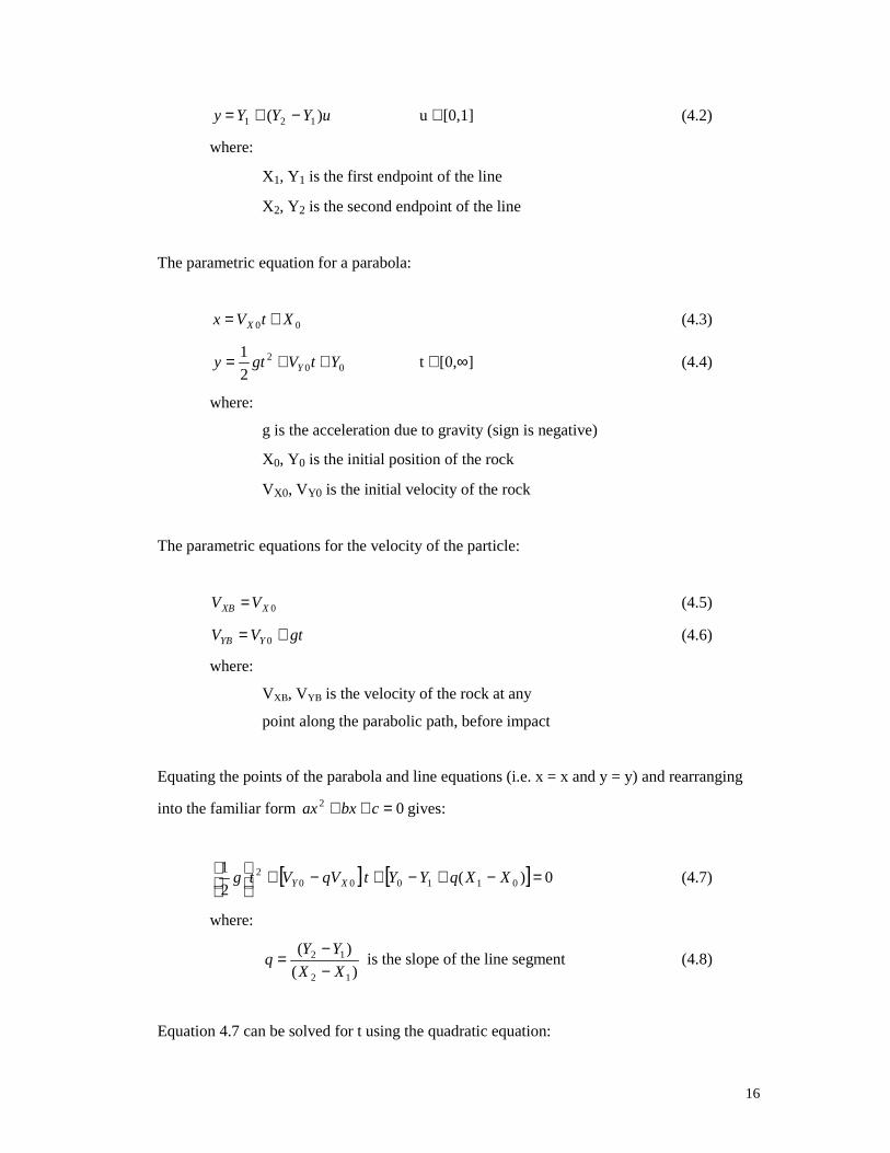
The parametric equation for a line:
uXXXx )( 121 −+= (4.1)
16
uYYYy )( 121 −+= u ∈[0,1] (4.2)
where:
X1, Y1 is the first endpoint of the line
X2, Y2 is the second endpoint of the line
The parametric equation for a parabola:
00 XtVx X += (4.3)
002
2
1YtVgty Y ++= t ∈[0,∞] (4.4)
where:
g is the acceleration due to gravity (sign is negative)
X0, Y0 is the initial position of the rock
VX0, VY0 is the initial velocity of the rock
The parametric equations for the velocity of the particle:
0XXB VV = (4.5)
gtVV YYB += 0 (4.6)
where:
VXB, VYB is the velocity of the rock at any
point along the parabolic path, before impact
Equating the points of the parabola and line equations (i.e. x = x and y = y) and rearranging
into the familiar form 02 =++ cbxax gives:
[ ] [ ] 0)(2
1011000
2 =−+−+−+
XXqYYtqVVtg XY (4.7)
where:
)(
)(
12
12
XX
YYq
−−
= is the slope of the line segment (4.8)
Equation 4.7 can be solved for t using the quadratic equation:

17
a
acbbt
2
42 −±−= (4.9)
where:
ga2
1= (4.10)
00 XY qVVb −= (4.11)
)( 0110 XXqYYc −+−= (4.12)
During each pass through the algorithm, the parabola formed by the rock trajectory is
checked with every segment of the slope and with every barrier. All of the slope segments
and barriers that have a valid intersection with the parabola are inserted into a list. The list is
then sorted by the value of the t parameter to determine the correct intersection.
Once the correct intersection is determined, the velocity just prior to impact is calculated
according to equations 4.5 and 4.6. These velocities are transformed into components normal
and tangential to the slope according to:
)sin()()cos()( θθ XBYBNB VVV −= (4.13)
)cos()()sin()( θθ XBYBTB VVV += (4.14)
where:
VNB, VTB are the velocity components of the rock, before impact,
in the normal and tangential directions, respectively
θ is the slope of the line segment
The impact is calculated, using the coefficients of restitution, according to:
NBNNA VRV = (4.15)
TBTTA VRV = (4.16)
where:
RN is the coefficient of normal restiution ∈[0,1]
RT is the coefficient of tangential restiution ∈[0,1]
VNA , VTA are the velocity components of the rock, after impact,
in the normal and tangential directions, respectively

18
The post-impact velocities are transformed back into horizontal and vertical components
according to:
)cos()()sin()( θθ TANAXA VVV += (4.17)
)cos()()sin()( θθ NATAYA VVV −= (4.18)
where:
VXA, VYA are the velocity components of the rock, after impact,
in the horizontal and vertical directions, respectively
Once the correct intersection is determined and the velocities have been calculated, all of the
data collectors are checked for intersection with the parabola (in a manner similar to checking
the slope segments). Any data collector with a parametric value (the value of t) less than the
value of the actual intersection is informed of the rock’s trajectory. The location, velocity
and kinetic energy of the rock, at the moment it passes the data collector, are recorded by the
data collector.
The velocity of the rock is then calculated and compared to VMIN. If it is greater than VMIN
the process starts over again, with the search for the next intersection point. If the velocity is
less than VMIN the rock can no longer be considered a particle, and is sent into the sliding
algorithm.
4.5 Sliding Algorithm
The sliding algorithm is used to calculate the movement of the rocks after they have exited
the projectile algorithm. The rocks can slide on any segment of the slope and on any barrier.
For the purpose of the sliding algorithm, the slope segment or barrier that the rock slides on,
consists of a single straight-line segment that has properties of slope angle (θ) and friction
angle (φ). The friction angle can be specified by a constant value or sampled from a random
distribution.
The rock can begin sliding at any location along the segment and may have an initial velocity
that is directed upslope or downslope. Only the velocity component tangential to the slope is
considered in the equations.

19
Once the sliding is initiated, the algorithm used depends on whether the initial velocity is
upslope or downslope. The algorithm used when the initial velocity is downslope will be
explained first.
4.6 Sliding Downslope
When the initial velocity of the rock is downslope (or zero) the behaviour of the rock depends
on the relative magnitudes of the friction angle (φ) and the slope angle (θ).
θ = φ If the slope angle is equal to the friction angle, the driving force (gravity) is equal to
the resisting force (friction) and the rock will slide off the downslope end of the segment,
with a velocity equal to the initial velocity (i.e. VEXIT = V0). There is a special case when
V0 = 0; in this case, the rock does not move, and the simulation ends.
θ > φ If the slope angle is greater than the friction angle, the driving force is greater than
the resisting force and the rock will slide off the downslope endpoint with an increased
velocity. The speed with which the rock leaves the slope segment is calculated by:
sgkVVEXIT 220 −= (4.19)
where:
VEXIT is the velocity of the rock at the end of the segment
V0 is the initial velocity of the rock, tangential to the segment
s is the distance from the initial location to the endpoint of the segment
g is the acceleration due to gravity (-9.81m/s/s)
k is )tan()cos()sin( φθθ −±
where:
θ is the slope of the segment
φ is the friction angle of the segment
± is + if the initial velocity of the rock is downslope or zero
± is − if the initial velocity of the rock is upslope

20
θ < φ If the slope angle is less than the friction angle, the resisting force is greater than the
driving force and the rock will decrease in speed. The rock may come to a stop on the
segment, depending on the length of the segment and the initial velocity of the rock.
Assuming that the segment is infinitely long, a stopping distance is calculated. The distance
is found by setting the exit velocity (VEXIT) to zero in equation 4.19 and rearranging:
gk
Vs
2
20= (4.20)
The distance from the initial location of the rock to the end of the segment is calculated. If
the stopping distance is greater than the distance to the end of the segment, then the rock will
slide off of the end of the segment. In this case, the exit velocity is calculated using equation
4.19. If the stopping distance is less than the distance to the end of the segment then the rock
will stop on the segment and the simulation is stopped. The location where the rock stops is a
distance of s downslope from the initial location.
4.7 Sliding Upslope
When sliding uphill both the frictional force and the gravitational force act to decrease the
velocity of the particle. Assuming that the segment is infinitely long, the particle will
eventually come to rest. The stopping distance is calculated using equation 4.20 and the
distance from the initial location of the rock to the upslope end of the segment is calculated.
If the stopping distance is greater than the distance to the end of the segment, the rock will
slide off of the end of the segment. In this case, the exit velocity is calculated using equation
4.19. If the stopping distance is less than the distance to the end of the segment the rock
comes to rest and the simulation is stopped.
If the rock slides up and stops it is then inserted into the downslope sliding algorithm. If the
segment is steep enough to permit sliding (i.e. θ > φ) then the rock will slide off the bottom
end of the segment. If the segment is not steep enough, then the location where the rock
stopped moving (after sliding uphill) is taken as the final location and the simulation is
stopped.

21

22

23

24
5. Numerical Instabilities
A lot of time and effort was required to solve the numerical instability problems in RocFall.
This chapter outlines some of the difficulties that were encountered when the particle
algorithm was implemented and the solution to those difficulties.
It is the author’s experience that writing an engineering program that works ninety five
percent of the time (a few situations not being handled properly) requires less than half of the
time and effort required to write a program that handles all of the situations properly. It is
important for a program that performs probabilistic simulations to work correctly in all cases.
Since each simulation has a slightly different outcome, and hundreds of simulations are
performed, a problem that occurs only once in a thousand simulations, will be noticed very
quickly.
5.1 Impossible situations
It is trivial to construct a case that is analytically valid (if not realistic) that could cause an
unsuspecting rockfall algorithm to continue indefinitely. For example, dropping a rock with
zero initial velocity onto a horizontal surface with RN = 1 would cause the rock to bounce up
and down − forever. This would cause the program to enter an endless calculation loop, and
stop responding to the user (otherwise known as a “crash”). While this example is contrived,
it is possible for the user of the program to inadvertently specify a similar situation.
Since the goal was to construct a robust program, this possibility of this situation, and similar
situations, was handled. Each rock is given a certain amount of real time (not to be confused
with simulation time, which will usually be much longer) to finish all of its calculations.
Since the amount of real time permitted for the calculations (approximately 10 s) is many
times larger than the typical solution time (approximately 0.02 s) whenever a simulation
“time’s out” the reason is almost always that the conditions specified are “impossible” and
convergence (the rock stopping) will never occur.

25
5.2 Numerical instabilities
One of the equations used to find the parabola-line intersection (equation 4.8) is unstable in
two situations (the instability is caused by the (X2 - X1) term in the denominator). The first
instability is encountered when the length of the line segment approaches zero. This problem
was solved by the forcing the program user to enter geometry such that each of the slope
segments is at least 1 mm in length.
The second instability is encountered when the line segment is vertical. Noting that the
parameter u can be removed from equation 4.1 when the line is vertical solved this problem.
When the parameter u is removed and the horizontal location is equated (i.e. x = x) with
equation 4.3 (the parabola equation), these equations can be solved for t.
0
01 )(
XV
XXt
−= (4.21)
The solution is now stable, for all cases except when the line is vertical and the rock has zero
initial horizontal velocity (VX0). When this occurs, there is no intersection between the
parabola and the line, and the instability is avoided.
The non-parametric versions of the parabola-line intersection were unstable for horizontal
velocities close to zero, which is a much more common occurrence than vertical slope
segments. This is another reason why the parametric versions of the equations are superior to
the slope, y-intercept form of the equations.
5.3 Machine Error
When equation 4.9 (the quadratic equation) is solved in the projectile algorithm the two roots
represent the starting point and ending point of the trajectory. A difficulty presents itself
because “machine error” will cause the root at the beginning of the trajectory to have a
parameter that is not exactly zero. When the bounce-height becomes extremely small, it can
become difficult to determine which root represents the beginning and which represents the
end. This difficulty was solved by offsetting the rock slightly below the segment, before each
trajectory, and taking the smallest positive root as the beginning point.

26
6. Recommendations
RocFall is an ongoing project. While the user-interface of the program can always be
improved, these recommendations focus on the calculation aspect of the program. The
recommendations are listed in order of desirability:
1. Gathering of empirical data for the coefficients of restitution
The outcome of a rockfall simulation is very dependent on the values used for the coefficients
of restitution. Unfortunately, appropriate values are not always well known and a lot of time
is usually spent determining what values should be used. Gathering a large sample of
previously used values in one location, similar to the work of Tomory (1997), would be
extremely useful. Gathering this data would require a substantial amount of time and effort.
2. Mass-based “plasticity” function for the coefficient of restitution
This would involve varying the coefficient of restitution based on the mass of the rock (i.e.
more massive rocks would use lower coefficients of restitution when the impact was
calculated). This would not require much work to implement.
3. “Breakable” barriers
This would require very little effort to add to the current program (in fact, most of the code
has already been written). The reason it was not added is that the outgoing velocity (after the
rock has passed through the barrier) is difficult to define. It was thought that the velocity
vector of the rock would be changed (tending towards the normal of the barrier, perhaps).
Further research into this behaviour should be performed before this feature is added.
4. Three-dimensional particle analysis
This would require a large amount of effort, but is within the realm of possibility. The factor
limiting the usefulness of this type of model would likely be the lack of input data (i.e. this
would require a large number of cross sections, which might not be available).
5. Consider angular velocity and/or shape effects in the particle model
Although desirable, this would require re-writing and re-verifying the entire calculation
section of the program. This would require a substantial amount of work.

27
7. Conclusion
7.1 Final Product
The final product of this work is the program RocFall. RocFall is a robust, easy-to-use
program that is capable of simulating rockfalls on a wide variety of slope geometries, and has
been used by dozens of engineers over the course of the last six months. The implementation
of the particle analysis is extremely robust and has proven to be stable for all of the realistic
and pathological cases that have been attempted.
The goal of this thesis was to create a tool to assist engineers with the probabilistic analysis of
rockfalls and the design of remedial measures. RocFall meets these objectives.
7.2 Verification
Essential to the use of a computer program in engineering practice, this thesis presents a
thorough verification of the program’s output. This verification can be found in appendix A.
The verification was placed in an appendix because it is lengthy and it was meant to be
readable separate from the body of the thesis. This was done so that an engineer that is using
the program can refer to the verification, without having to read the entire thesis.
7.3 The Program
RocFall was written with Microsoft Visual C++ 5.0 using the Microsoft Foundation Classes
(MFC) class library. The complete RocFall program consists of slightly more than 26,000
lines of code contained in approximately 400 files. It would be impractical, and of little
value, to print out and include all of these files, as this would expand the thesis by more than
800 pages. Instead, only those files that relate to the particle analysis have been included in
this thesis. A thorough explanation of the calculation engine used by the particle analysis,
and a guide to its use, is presented in appendix B.

28
ReferencesAnten, H. and Rorres, C. Elementary Linear Algebra 6th Edition. John Wiley & SonsInc., New York.
Azzoni, A., Barbera, G.L., Zaninetti, A., Analysis and Prediction of Rockfalls Using aMathematical Model. Int. J. Rock. Mech. Min. Sci & Geomech, Elsevier Science Ltd. GreatBritain, Vol 32 No 8 pp 709-724 1995.
Canale R.P., Charpa, S.C., Numerical Methods for Engineers. Second Edition. McGraw-HillPublishing Company. New York.
Corkum, B. 1986. The Discrete Element Method in Geotechnical Engineering. Department ofCivil Engineering, University of Toronto, Toronto, Ontario, Canada.
Hoek, E. 1984. Acceptable Risks and Practical Decisions in Rock Engineering. Departmentof Civil Engineering, University of Toronto, Toronto, Ontario, Canada.
Hoek, E. 1987. RockFall - A Program for the Analysis of Rockfalls from Slopes. Departmentof Civil Engineering, University of Toronto, Toronto, Ontario, Canada.
Hoek, E. 1994. Course Notes for Rock Engineering (CIV 529S). Evert Hoek ConsultingEngineer Ltd, North Vancouver, British Columbia, Canada.
Hoek, E. 1996. Report on Tuen Mun Highway Widening Shui On - Balfour Beatty JVContract Hong Kong. Evert Hoek Consulting Engineer Ltd, North Vancouver, BritishColumbia, Canada.
Pfeiffer, T.J., and Bowen, T.D., Computer Simulation of Rockfalls. Bulletin of theAssociation of Engineering Geologists Vol. XXVI, No. 1, 1989 p 135-146.
Ross, Sheldon M., 1987. Introduction to Probability and Statistics for Engineers andScientists. John Wiley & Sons Inc., New York.
Salvador, Tony. 1989. Rockfall. University of Toronto, Toronto, Ontario, Canada.
Santo, A. and Budetta, P. 1994. Morphostructural Evolution and Related Kinematics ofRockfalls in Campania (southern Italy): A case study. Engineering Geology 36 ElsevierScience Ltd. Great Britain, pp.197-210.
Stevens, W. 1996. Rockfall 4.0 Software for the Analysis of Falling Rocks on a Steep Slope.B.A.Sc. Thesis. Department of Civil Engineering, University of Toronto, Ontario, Canada.
Stevens, W. 1997. The rockfall files: A guide to the On-going Investigation of Rockfalls atthe University of Toronto. Department of Civil Engineering, University of Toronto, Toronto,Ontario, Canada.
Tomory, Paul B. 1997. Analysis of Split Set Bolt Performance. M.A.Sc. Thesis. Departmentof Civil Engineering, University of Toronto, Toronto, Ontario, Canada.