robustness of idle-throttle continuous descent …staff.itee.uq.edu.au/pal/papers/atio09.pdf ·...

Robustness of Idle-throttle

Continuous Descent Approach Trajectories

against Modified Timing Requirements

Peter A. Lindsay∗ and Colin Ramsay†

ARC Centre for Complex Systems, The University of Queensland, Brisbane 4072, Australia

Miguel Vilaplana‡, Javier Lopez Leones‡ and Enrique Casado‡

Boeing Research & Technology Europe, Madrid, Spain

Paul C. Parks§

The Boeing Company, Seattle, WA, USA

This paper reports on a study of the robustness of Continuous Descent Approach (CDA)trajectories in the face of late changes to the Required Time of Arrival (RTA). We demon-strate a method for determining limits on how much the RTA can be modified, as a functionof notification lead-time, without significantly impacting on optimality of the CDA. Ourfocus is on the period between Top Of Descent (TOD) from cruise level and arrival at ametering fix. The aim is to help determine how flexible airspace constraints would needto be in order to accommodate robust CDA. The Aircraft Intent Description Language(AIDL) is used as the modelling language.

I. Introduction

In this paper we report the results of a study of the robustness of Continuous Descent Approach (CDA)trajectories in the face of late changes to the Required Time of Arrival (RTA). We demonstrate a method

for determining limits on how much the RTA can be changed, as a function of notification lead-time, withoutsignificantly impacting on the main goal of ‘ideal’ CDA. We define an ideal CDA as an idle-throttle descentalong a fixed lateral approach path with a planned speed schedule. (The reasoning behind our definition isexplained below; other definitions are possible.1) Such trajectories are desirable for many different economicand environmental reasons, including fuel use, emissions and noise abatement.

Underlying the motivation for this study is the assumption that, as a result of improved trajectory predic-tion and trajectory conformance, in the ideal future trajectory-based ATM (Air Traffic Management) System,most of the current tactical ATC approach-sequencing practices will have been replaced by a mechanismfor adjusting RTAs, with supporting processes for recalculating the affected trajectories from knowledge ofuser preferences.1–4 It is thus vital to understand the key parameters of such a mechanism when designingsupporting tools and procedures for CDA: namely, according to how soon one realises that a change to anRTA may be required, how much change is feasible without significant loss of the benefits of CDA, and whatvariation is associated with the revised trajectory.

∗Professor of Systems Engineering, School of Information Technology and Electrical Engineering, The University of Queens-land, Brisbane 4072, Australia.

†Research Fellow, ARC Centre for Complex Systems, The University of Queensland, Brisbane, Australia.‡Advanced Trajectory Technologies, Boeing Research and Technology Europe, Madrid, Spain.§Lead Engineer – Planning and Decision Aids, Networked Systems Technology, Boeing Research and Technology, The Boeing

Company, Seattle, WA, USA. Member.

1 of 24

American Institute of Aeronautics and Astronautics

I.A. Background

A number of studies1,5, 6 have considered the final approach segment and Terminal Manoeuvring Area (TMA)aspects of CDA, but we focus on the approach phase here, between Top of Descent (TOD) and arrival ata metering fix. Our ultimate aim is to inform the redesign of airspace to enable CDA to be flown with aslittle intervention as possible (in this case, just one single speed adjustment), by understanding what air-sideflexibility is possible.

Other studies4 have considered the issue of modifying RTA while in the flight is in cruise phase, which isclearly the preferred option if possible since adjustment can be made relatively easily and cheaply. However,for the foreseeable future it is inevitable that adjustments will sometimes need to be made to the aircraft’sRTA once a descent from cruise level has been initiated. This would typically be due to ‘last minute’events that could not always be predicted accurately, such as runway activity, spacing adjustments, anddeconfliction with departing aircraft. This prompts the question of how much flexibility exists after descenthas begun.

Current tactical ATCo (Air Traffic Controller) approaches to modifying approach trajectories to insertdelay into a trajectory include vectoring and holding, both of which are undesirable because they involveextra fuel burn, noise and workload for flight crew and controllers. Our approach is instead to check to whatdegree the aircraft’s FMS (Flight Management System) can use elevator control to accommodate the change,keeping a fixed lateral path and modifying the speed schedule. A steeper (hence faster) descent will resultin the aircraft passing the fix earlier; a shallower descent will make it pass later. Of course this will result ina change to the altitude profile, and a change to the height at which the fix is passed, but (within limits) weexpect this to be an acceptable compromise. Where path lengthening is feasible, this could be incorporatedinto a shallower descent, in order to insert a delay without needing to change the height target – but thatwill be left to a later study. For now we are interested in the extent to which it is feasible to achieve the newRTA while following a fixed lateral path, and the consequent effect on the speed and height at which the fixis passed.

Put in a different way, the objective is to determine what values of ∆RTA and lead-time will require pathlengthening and/or holding in addition to speed control.

Note that we are considering ideal idle-throttle CDAs as a way of minimising fuel use/emissions and ad-dressing noise abatement. This is by contrast with CDAs that follow a fixed pre-determined three-dimensionalgeometrical profile (VNAV-Path descent). Although the latter are certainly an improvement on stepped ap-proaches, they become suboptimal if the RTA changes, since engine control is required in order to maintainthe vertical profile. In our approach the throttle remains at idle throughout descent, until the metering fixis passed; what happens after that is outside the scope of our immediate study (but see Section III.A belowfor more discussion).

I.B. The Modelling Approach

Our study was performed using a prototype trajectory modelling tool developed by BRTE. The tool usesthe Aircraft Intent Description Language (AIDL)7 as the input format.

AIDL is a formal language developed by BRTE to describe and exchange aircraft intent information. Inthe context of trajectory prediction, aircraft intent means an unambiguous description of how the aircraftis intended to be operated within a certain time interval. AIDL is characterized by an alphabet and agrammar. The alphabet is formed by a set of instructions, which are conceptual elements used to modelthe basic commands, guidance modes and control strategies at the disposal of the pilot/FMS, to directthe operation of the aircraft. The AIDL grammar is defined in such a way that a valid AIDL sentenceis guaranteed to unambiguously define the aircraft’s trajectory, given a suitable set of initial conditions,aircraft performance model and model of the environment. This makes AIDL ideally suited for use as theinput language for a wide range of real-time/fast-time simulators and trajectory prediction tools.

Previously AIDL has been considered as a potential tool for transfer of aircraft intent information betweenair- and ground-based systems, for example to examine the conditions under which conflicts can arise.8 Ourapplication demonstrates its use for modelling and testing new concepts of operation such as CDA.

For our study, AIDL sentences were developed to describe the baseline CDA scenarios and their variants,including different intervention lead-times and revised speed schedules. Then BRTE’s prototype trajectory-computation tool was used in a series of experiments to calculate the effect on the time, height and speedat which the metering fix gets passed. The effects of a number of different environmental, aircraft and

2 of 24


flight-deck factors on the results were also modelled, using variants of the baseline AIDL sentences.

I.C. Structure of this Paper

The remainder of this paper is organised as follows. Section II describes AIDL in more detail. Section IIIdescribes the CDA scenario on which the approach is illustrated: namely, a Boeing 737-800 (B738) seriesaircraft performing an idle-throttle Mach/CAS descent from cruise level to pass over a metering fix at agiven time. Some time after TOD the flight crew modify the aircraft’s Mach/CAS speed schedule values,and the aircraft’s trajectory gets modified accordingly: the aircraft continues to fly at idle throttle andelevator controls are used to achieve the new speed schedule. Section IV presents the main results of theB738 study, in terms of the effect that different speed schedule values have on the time, height and speed atwhich the aircraft passes the fix.

Section V investigates the sensitivity of the results to various different flight factors, including environ-mental factors (barometric pressure and wind), aircraft factors (weight), and flight deck factors (cruise heightand initial speed schedule). We assume that these variations are known prior to descent and incorporatedinto the calculation of the TOD point and original RTA. It would be a straightforward matter to modify ourmodels to treat them instead as uncertainty factors if desired (individually or collectively), but we have notdone so here.

Section VI summarises the results of a second study, involving a Boeing 777-300 (B773) series aircrafton a longer descent, by way of comparison.

I.D. Acronyms

AIDL Aircraft Intent Description Language CDA Continuous Descent Approach

APM Aircraft Performance Model EM Environmental Model

ATCo Air Traffic Controller FMS Flight Management System

ATM Air Traffic Management RTA Required Time of Arrival

B738 Boeing 737-800 ∆RTA net change in RTA

B773 Boeing 777-300 TAS True Air Speed

BRTE Boeing Research & Technology Europe TCI Trajectory Computation Infrastructure

CAS Calibrated Air Speed TOD Top Of Descent

II. The Aircraft Intent Description Language (AIDL)

This section describes the modelling language used in the study. As noted above, AIDL is characterized byan alphabet and a grammar. The alphabet is formed by a set of instructions, which are conceptual elementsused to model the basic commands, guidance modes and control strategies at the disposal of the flight crewand/or FMS, to direct operation of the aircraft. The grammar describes rules for assembling instructions intosets and sequences, in order to describe aircraft intent. A valid AIDL sentence describes a unique 4D aircrafttrajectory when interpreted in an appropriate Trajectory Computation Infrastructure (TCI) environment.9

Each of these aspects is described in more detail below.

II.A. AIDL instructions

Table 1 lists the 34 instruction types currently supported by AIDL. There are AIDL instructions for alldifferent aspects of aircraft motion: lateral and vertical motion, speed, energy, engine and configurationsettings. They are grouped into the following classes:

• Set instructions model control and configuration transients. Typically, a set instruction captures theevolution of a state or configuration variable from an initial to a target value according to an externallydefined function (e.g., the APM may define the transients of flap deployment).

• Law instructions model closed-loop control and guidance laws. Typically, these instructions capturethe evolution of a control or state variable as a function of one or more state variables (e.g., a lawdescribing the evolution of the Mach number as a function of the altitude).

3 of 24


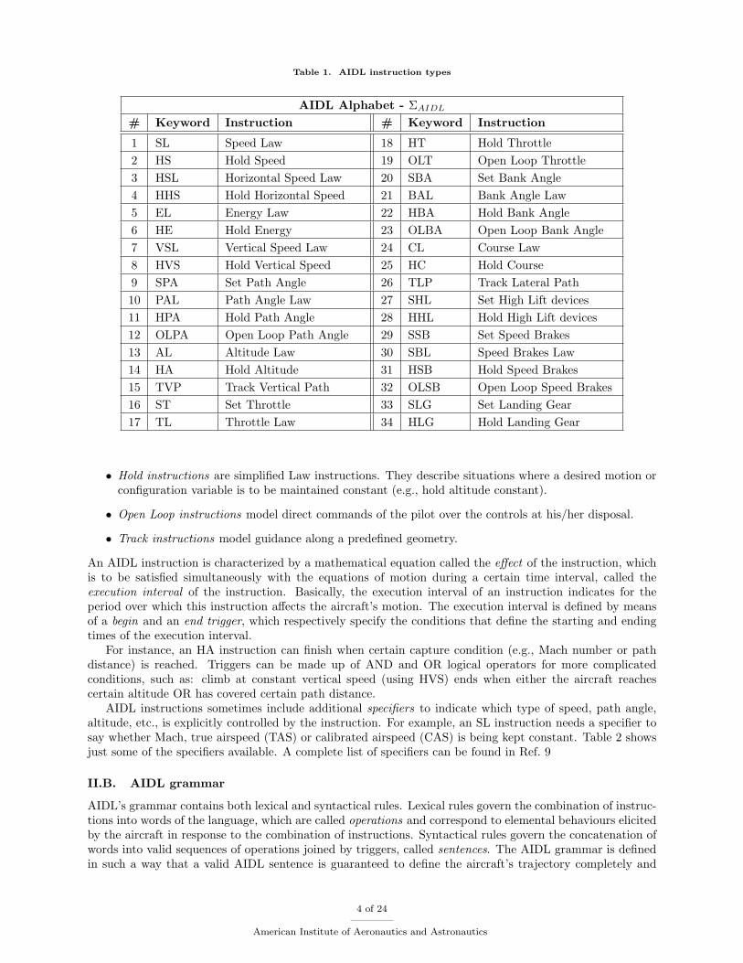
Table 1. AIDL instruction types

AIDL Alphabet - ΣAIDL

# Keyword Instruction # Keyword Instruction

1 SL Speed Law 18 HT Hold Throttle

2 HS Hold Speed 19 OLT Open Loop Throttle

3 HSL Horizontal Speed Law 20 SBA Set Bank Angle

4 HHS Hold Horizontal Speed 21 BAL Bank Angle Law

5 EL Energy Law 22 HBA Hold Bank Angle

6 HE Hold Energy 23 OLBA Open Loop Bank Angle

7 VSL Vertical Speed Law 24 CL Course Law

8 HVS Hold Vertical Speed 25 HC Hold Course

9 SPA Set Path Angle 26 TLP Track Lateral Path

10 PAL Path Angle Law 27 SHL Set High Lift devices

11 HPA Hold Path Angle 28 HHL Hold High Lift devices

12 OLPA Open Loop Path Angle 29 SSB Set Speed Brakes

13 AL Altitude Law 30 SBL Speed Brakes Law

14 HA Hold Altitude 31 HSB Hold Speed Brakes

15 TVP Track Vertical Path 32 OLSB Open Loop Speed Brakes

16 ST Set Throttle 33 SLG Set Landing Gear

17 TL Throttle Law 34 HLG Hold Landing Gear

• Hold instructions are simplified Law instructions. They describe situations where a desired motion orconfiguration variable is to be maintained constant (e.g., hold altitude constant).

• Open Loop instructions model direct commands of the pilot over the controls at his/her disposal.

• Track instructions model guidance along a predefined geometry.

An AIDL instruction is characterized by a mathematical equation called the effect of the instruction, whichis to be satisfied simultaneously with the equations of motion during a certain time interval, called theexecution interval of the instruction. Basically, the execution interval of an instruction indicates for theperiod over which this instruction affects the aircraft’s motion. The execution interval is defined by meansof a begin and an end trigger, which respectively specify the conditions that define the starting and endingtimes of the execution interval.

For instance, an HA instruction can finish when certain capture condition (e.g., Mach number or pathdistance) is reached. Triggers can be made up of AND and OR logical operators for more complicatedconditions, such as: climb at constant vertical speed (using HVS) ends when either the aircraft reachescertain altitude OR has covered certain path distance.

AIDL instructions sometimes include additional specifiers to indicate which type of speed, path angle,altitude, etc., is explicitly controlled by the instruction. For example, an SL instruction needs a specifier tosay whether Mach, true airspeed (TAS) or calibrated airspeed (CAS) is being kept constant. Table 2 showsjust some of the specifiers available. A complete list of specifiers can be found in Ref. 9

II.B. AIDL grammar

AIDL’s grammar contains both lexical and syntactical rules. Lexical rules govern the combination of instruc-tions into words of the language, which are called operations and correspond to elemental behaviours elicitedby the aircraft in response to the combination of instructions. Syntactical rules govern the concatenation ofwords into valid sequences of operations joined by triggers, called sentences. The AIDL grammar is definedin such a way that a valid AIDL sentence is guaranteed to define the aircraft’s trajectory completely and

4 of 24


Table 2. Some AIDL instruction specifiers

Instructions Parameter Keyword Units

SL, HS Mach number MACH –

calibrated airspeed CAS kt

true airspeed TAS kt

indicated airspeed IAS kt

HA geopotential pressure altitude PRE ft

geometric altitude GEO ft

TL max climb regime MCMB –

low idle throttle regime LIDL –

go around regime GA –

throttle control parameter THRO –

thrust coefficient CT –

unambiguously over the corresponding execution interval, given a suitable set of initial conditions, aircraftperformance model and model of the environment.

AIDL is based on the principle that, during any given time interval, the trajectory of an aircraft (consid-ered as a mass-point) is determined by closing the three degrees of freedom (3-DOF) of the aircraft motion.9

Under certain assumptions about the underlying aircraft performance model, this is done mathematically byadding three constraints (which can be expressed as algebraic equations) to the three ordinary differentialequations (ODEs) that govern the aircraft’s motion. Certain AIDL instructions (called motion instructions)each close a single DOF of aircraft motion. The time interval during which each instruction is active iscontrolled through the trigger conditions.

Not any combination of three instructions results physically compatible according to the laws that governthe flight dynamics of an aircraft. However, it has been found that the rules governing valid combinationsadmit the structure of a formal regular language (in the sense of the Mathematical Theory of Formal Lan-guages). The AIDL grammatical rules ensure that grammatically valid combinations of motion instructions,together with suitable initial conditions and trigger conditions, possess a unique 4D trajectory-segment so-lution when combined with suitable models of aircraft performance and environmental conditions (see nextsection).9 The AIDL alphabet of instructions covers a very wide range of aircraft motion elements under awide range of different possible aerodynamic configurations, including activation of high-lift devices and/orspeed brakes, and landing gear status. AIDL also provides features to help trajectory modelling tasks bydelegating to the TCI the location of auto and default parameter values. Moreover, the AIDL also cap-tures current and advanced optimal flight modes. These features make AIDL ideal for platform-independentspecification of aircraft intent.

See Fig. 2 below for an example of aircraft intent expressed graphically using AIDL, together with verticaland horizontal views of the corresponding trajectory.

II.C. Trajectory computation for AIDL

As noted above, a grammatically correct AIDL sentence defines a unique 4D aircraft trajectory segment fora given set of initial conditions when interpreted in a suitable model of aircraft performance and model ofenvironmental conditions. Boeing RTE have developed a prototype tool-set for calculating this trajectory,based on the architecture in Figure 1. The general characteristics required of the different components ofthe Trajectory Computation Infrastructure (TCI) are described briefly below.

The Aircraft Performance Model (APM) is based on BADA models,11 which provide data for predictionof the aircraft performance. The prototype tool-set used in our experiments included means for calculatingforces associated with aerodynamic drag, lift, engine thrust and weight, parametrically modelled as functionsof the atmosphere conditions (pressure, temperature and wind), aircraft position, aircraft true airspeed andaircraft type. (The prototype tool supports Boeing 737-800 and 777-300 series aircraft types.) It also includeda series of parametric models which capture the primitive ways in which an aircraft can be operated (e.g.

5 of 24


Figure 1. Trajectory Computation Infrastructure (TCI) for AIDL

the way it: deploys and retracts high-lift devices, spoilers or landing gear; holds altitude, speed, pathangle and bank angle; rolls and pitches; etc) and parametric models which restrict aircraft behavior to staywithin appropriate limits for safeguarding operation of the aircraft and limiting equipment degradation (e.g.speed limitations, weight limitations, load factor limitations, etc), as functions of a set of aircraft-specificparameters.

The Environmental Model (EM) provides means for predicting the environmental conditions (tempera-ture, atmospheric pressure and wind) that the airplane would encounter as it flew its trajectory, as a functionof spatial position and time.

The TCI used in our experiments was able to interpret AIDL expressions as sets of algebraic differentialequations and numerically integrate them for given initial conditions using the APM and EM. The outputwas a sequence of state vector values sampled at a discrete set of time instants. It also included supportfor certain forms of implicit parameters in AIDL trigger conditions, such as being able to determine theappropriate point for Top Of Descent (TOD) in order to satisfy a given Required Time of Arrival (RTA) atan approach fix, or to calculate the point at which to transition smoothly from constant Mach to constantCAS during descent. It does this by iterating calculations and backtracking. We made good use of thesefeatures in our experiments, as discussed further in Section III below.

6 of 24


III. Case Study I: Boeing 737-800

This section describes the scenario on which the approach is illustrated: a Boeing 737-800 aircraft performingan idle-throttle Mach/CAS Continuous Descent Approach (CDA) from cruise level to pass over a meteringfix at a given Required Time of Arrival (RTA) and given height and speed. Sometime after descent hascommenced, ATC notifies the aircraft that the RTA needs to be changed. The question is, by how much canthe RTA feasibly be modified, while still maintaining idle throttle, a constant Mach/CAS regime and cleanconfiguration, and just using elevator controls to achieve the new speed schedule? (That is, using a steeper– thus faster – descent to achieve an earlier RTA, or a shallower – thus slower – descent to achieve a laterRTA.) Of course, the answer will depend in part on how much lead-time is given. Since the revised descenttrajectory will also result in the fix being passed at a new height and speed, the answer will also dependon whether these new values are tolerable, as well of course as whether the remainder of the trajectory isacceptable. As noted above, we restrict ourselves to calculating the affect that modifying the speed schedulehas on the time, height and speed at which the fix is passed.

Table 3. Baseline scenario for B738 study

Initial conditions Final conditions

weight height Mach CAS TAS height CAS TAS

(tonne) (FL) (kt) (kt) (FL) (kt) (kt)

58 350 0.763 258 440 100 280 323

Section III.A explains the context of the study and the reasons behind some of the assumptions used.Section III.B describes the baseline (uninterrupted) scenario and how it was modelled in AIDL. Section III.Cdescribes how interrupted descents (i.e., CDAs where the speed schedule was modified at a given time) weremodelled in AIDL, and how the resulting effects on time, height and speed at the metering fix were calculated;the results are presented in Section IV below. Section V describes how the methodology was modified toinvestigate sensitivity of the results to a range of different flight factors. Section VI gives summary resultsfor a second scenario, involving a Boeing 777-300 aircraft descending from a higher cruise level.

III.A. Context

In order to keep the study manageable, and to report the results in a systematic manner, we made somesimplifying assumptions which will be explained here briefly.

The reason for considering idle throttle CDA was explained above: we wish to minimize fuel burn,emissions and (perhaps) noise. As noted above, using elevator controls to achieve a new RTA is howevergoing to result in a change to the height and speed at which the metering fix is passed. This will mean thatan aircraft operating procedure would need to be put in place to handle the rest of the descent trajectory,from the metering fix through to landing on the runway, to complement our proposed strategy. One suchprocedure is described in Ref. 3, for example. But these matters are outside the scope of our current study,and we focus simply on elucidating the size of the height and speed ‘errors’ that might result under ourapproach. (Note also that we are not assuming the use of any particular Flight Management System (FMS)mode on the aircraft: the purpose of the study is simply to investigate the implications of using speed controlto meet revised RTAs after TOD.)

Another simplifying assumption is that we consider just a single modification to the descent trajectory,and assume that speed schedules are kept constant before and after the trajectory change. The reason forconsidering just a single change was to keep the experiments manageable; however, the methodology couldeasily be adapted to more complex situations, such as where further constraints are imposed (additionalto, or in place of, the revised RTA requirement), such as speed or height limits (upper and/or lower). Themotivation for keeping speed schedules constant is that this is a typical ATC-related operating principlein many existing ATM systems, intended to facilitate maintenance of ATCo situation awareness, and weanticipate that this principle is likely to remain important – if not become even more important – in future.(The new speed schedule would need to be conveyed to the ATM System of course, and checked for conflictsbefore a revised clearance would be granted, but such matters are outside the scope of our study.)

7 of 24


Finally, we have described our study in terms of modifying the trajectory to achieve a revised RTA. Thereis an underlying assumption that time-based management of air traffic at key points (“metering” at fixes)is, and will remain, important in high traffic-density ATM. But in lower density ATM it may be preferableto allow the on-board FMS to calculate a revised speed schedule which is optimal for that flight overall(through to landing), and to inform ATC of the desired revision to RTA. But that is outside the currentstudy; the modelling methodology could be modified to cater for such a situation if desired.

III.B. Baseline Scenario

This section describes the baseline (uninterrupted) CDA scenario and how it was modelled in AIDL. Theaircraft descends from cruise level FL350 and cruise speed Mach.763 to pass over a metering fix at heightFL100 (see Table 3). The aircraft’s initial weight is 58 tonnes and the aircraft is in a clean configurationthroughout descent (i.e., no speed brakes or high-lift devices deployed, and landing gear retracted). Thefix’s coordinates are 25◦ N and 15◦ W, and the aircraft’s lateral path is a great circle, at a constant bearingof 180◦ (i.e., due South). The CAS value of the speed schedule is 280 kt. The standard atmospheric modelwas used,10 with a temperature of 15 ◦C at sea level and no wind.

OP#1

HS(MACH)

TL(LIDL)

TLP

HS(CAS)

HHL

HSB

HLG

O2

Great circle from O1 to O2

HA(PRE)

TOD

Transition Altitude

TOD

180ºO2

O1

O1

O2

A

Mach = 0.763

CAS= 280kt

vCAS=280kt A

Initial Conditions

Ver

tical

Ho

rizo

ntal

AIR

CR

AFT

TR

AJE

CTR

OY

OPERATIONS

Con

figur

atio

n

Pro

files

AIR

CR

AFT

INT

NE

T

Mot

ion

Pro

files

OP#2 OP#3

Figure 2. The baseline (uninterrupted) B738 CDA trajectory in AIDL

8 of 24


The AIDL representation of this baseline case is given in the top part of Fig. 2. The initial conditions canbe summarized as clean aerodynamic configuration at a geopotential pressure altitude of 35,000 ft with Machnumber M of 0.763. The initial HS (Hold Speed) and HA (Hold Altitude) instructions have their specifiershown within the instruction box. The HA operation concludes at point TOD, which is modelled by afloating trigger. At this point the power plant transitions to second operation OP#2 and then maintainsthe LIDL (Low Idle) regime, which is shown within the TL (Throttle Law) instruction. This causes theaircraft to start descent. The aircraft maintains its speed at Mach 0.763, represented by means of an HSinstruction with Mach as specifier. This instruction is active until the calibrated airspeed (CAS) is 280kt; atthis moment – called the transition altitude (TA) – the condition defining the floating trigger is satisfied andOP#2 ends. Thereafter the aircraft stops flying at constant Mach to continue at constant CAS of 280 kt(OP#3).

On the lateral path, the sequence consists of a single instruction, corresponding to following a great circlepath defined by the O1 and O2 way points, corresponding to the starting point and the meter fix lat/longcoordinates, respectively. This is specified using the TLP (Track Lateral Path) instruction with an intrinsicconstraint, defined in the box above the instruction. Finally, on the configuration threads the sequencerepresents the clean configuration state with the landing gear, high lift devices and speed brakes in retractedpositions (configuration instructions HLG, HHL and HSB respectively).

BRTE’s prototype AIDL-based trajectory computation tool was used to calculate where and when TODwould occur, using the standard BADA B738 performance characteristics.11 The tool calculated that TODwould occur 70 NM and 651 secs away from the fix. Likewise, the tool calculated that the Mach/CAStransition would take place 69 secs after TOD. The initial speed (Mach.763) equates to 440 kt True AirSpeed (TAS) and 258 kt CAS. The aircraft overflies the fix at 323 kt TAS. The trajectory computed by thetool for this case is called the reference run (or sometimes, the nominal case) in what follows.

III.C. Interventions to Modify RTA

For the purposes of analysis, we consider two types of modification to the trajectory during a Mach/CASdescent.

The first type, which we call a rescheduled CAS intervention, is where the CAS value of the speed scheduleis revised during the Mach phase of descent before the new CAS is reached. (The aircraft’s calibrated airspeedsteadily increases during a typical constant Mach descent.) The AIDL sentence representing this situationis almost exactly the same as before, except that the CAS value in the floating trigger (between operationsOP#2 and OP#3) is changed from 280 kt to the appropriate new value, and the floating trigger for TOD isreplaced by a value trigger, using the value of TOD computed from the reference run.

The second type of trajectory modification, which we call an altered CAS intervention, is where theCAS value of the speed schedule is revised during the CAS phase of descent. Fig. 3 illustrates how thisis modelled in AIDL. This involves adding a fourth operation (OP#4), in which a speed law is used withthe new value of CAS (250 kt in the example illustrated) triggered at time tc (B) and then held constantuntil the fix is overflown (O2). Note that this results in an instantaneous change in the value of CAS inthe corresponding equations of motion, which is clearly unrealistic in practice. We could remedy this bymaking some assumptions about how the flight crew would achieve the change in practice, and then modelit in AIDL and extract the results. If the speed change is done quickly enough though, we expect that theresults will not be very different from the ones obtained using our simplified approach.

A third possible scenario, where both the Mach and the CAS values are changed after descent hascommenced, was not considered in this study; nor was the case where the CAS value is revised during theMach phase but after the new CAS value has already been exceeded. The technique used for the altered CASinterventions could easily be adapted for these cases. However the time frames within which the interventionswould need to take place is quite short in both cases, so the results will not differ much from the other cases,while complicating the analysis somewhat.

Figure 4 shows the true airspeed (TAS) values calculated by the tool for three cases: the baseline referencerun (“nominal case”); a rescheduled CAS run where the CAS value has been changed to 300 kt during theMach phase (“300(R)”); and an altered CAS run where the CAS value has been altered to 260 kt with alead-time of 395 secs (“260(A)”). Figure 5 shows the pitch values for the same runs: this illustrates what theelevator controls actually do during the runs. Figure 6 shows the average ground speed for the same runs.Finally, Figure 7 shows the descent profile for the 3 comparison trajectories. In short, the 260(A) descent

9 of 24


OP#1

HS(MACH)

TL(LIDL)

TLP

HS(CAS)

HHL

HSB

HLG

O2

Great circle from O1 to O2

HA(PRE)

TOD

Transition Altitude

TOD

180ºO2

O1

O1

O2

A

Mach = 0.763

CAS= 280kt

vCAS=280kt A

Initial Conditions

Ver

tical

Ho

rizo

ntal

AIR

CR

AFT

TR

AJE

CTR

OY

OPERATIONS

Con

figur

atio

n

Pro

files

AIR

CR

AFT

INT

NE

T

Mot

ion

Pro

files SL(CAS=250kt)

tC B

OP#4

B

CAS= 250kt

Altered CAS

OP#2 OP#3

Figure 3. An example ‘altered CAS’ trajectory represented in AIDL

10 of 24


0 10 20 30 40 50 60 70 80300

320

340

360

380

400

420

440

460

distance [NM]

TA

S [k

t]

TAS vs distance

260(A)Nominal300(R)

Figure 4. TAS vs distance from TOD for 3 example B738 runs

0 10 20 30 40 50 60 70 80−5

−4.5

−4

−3.5

−3

−2.5

distance [NM]

Pitc

h [d

eg]

Pitch vs distance

260(A)Nominal300(R)

Figure 5. Pitch values for the 3 example B738 runs

11 of 24


0 10 20 30 40 50 60 70 80360

370

380

390

400

410

420

430

440

450

distance [NM]

dist

ance

/t [k

t]

distance/t vs distance

260(A)Nominal300(R)

Figure 6. Average ground speed values for the 3 example B738 runs

0 10 20 30 40 50 60 70 800.5

1

1.5

2

2.5

3

3.5x 10

4 Hp vs distance

distance [NM]

Hp

[ft]

300(R)260(A)Nominal

Figure 7. Descent profile for the 3 example B738 runs

12 of 24


is shallower and slower than the baseline (uninterrupted) CDA, whereas the 300(R) descent is steeper andfaster.

In Section IV below we vary the value of CAS used in the two different types of intervention and reportthe effect on the time as which the fix is overflown (∆RTA) and the associated changes in height and speedat which the fix is passed. In Section V we modify parameters in the initial conditions, Aircraft PerformanceModel and Environment Model to simulate variations in different flight factors, and rerun the experimentsin order to investigate the sensitivity of the results to those factors.

IV. Results

This section reports the results of the experiments to determine the effect that different speed schedulevalues have on the time, height and speed at which the aircraft passes the fix, according to the amount oflead-time given (see Section III for details). Here the Mach value is kept constant and a CAS value of 280 ktis used as the reference case. We report the results obtained by varying the CAS value of the modified speedschedule between 250 kt and 310 kt in steps of 10 kt in two cases, according to whether the CAS value ischanged during the Mach or CAS phase of Mach/CAS descent.

In what follows the “height error” (∆height) is reported as the difference between the height at whichthe fix is passed and the nominal height (10,000 ft) in pressure altitude, and “speed error” (∆speed) is thedifference in true airspeed from the nominal speed at which the fix is passed (323 kt). Figures reported arerounded as follows: time to the nearest whole second, speed to the nearest knot, and (pressure) height tothe nearest 10 ft.

IV.A. Rescheduled CAS Interventions

For the rescheduled CAS interventions, where the CAS value of the Mach/CAS descent is changed beforethe transition from the Mach regime, we varied the CAS value is varied from 260 kt to 310 kt. (The CASvalue at cruise is 258 kt, so values lower than this cannot be used, for the reasons given in Section III.C.)

Table 4. Effect of Rescheduled CAS interventions

Revised transition time lead-time ∆RTA height error speed error

CAS value (sec after TOD) (sec) (sec) (ft) (kt)

260 7 >644 26 2850 -10

270 39 >612 12 1450 -5

280 69 - 0 0 0

290 97 >582 -11 -1480 4

300 122 >582 -20 -2960 8

310 146 >582 -28 -4460 12

Table 4 summarizes the results for the different CAS values. It shows the net amount by which the time-at-fix would be altered (∆RTA) if the CAS value was revised after TOD, together with the correspondingnet change in the height and speed at which the fix would be passed. The ‘transition time’ column indicateshow long after TOD the Mach/CAS transition would occur. The ‘lead-time’ column indicates the minimumlead time required to allow a rescheduled CAS intervention to occur (i.e., net amount of time before theflight was originally scheduled to fly over the fix). Note that for CAS values lower than the nominal value(280kt), the lead-time is longer (i.e., the intervention needs to occur earlier in the Mach phase) since theCAS value is reached earlier. For CAS values higher than 280kt, on the other hand, the lead-time is 582(= 651-69) secs, since after this point the flight will have transitioned into the CAS phase of descent, anda “rescheduled CAS intervention” is no longer possible. Note that the actual time at which a rescheduledCAS intervention takes place does not affect the ∆RTA (etc) results, provided of course that the CAS valueis revised before the minimum lead-time is reached. Revising the CAS value after this time corresponds tothe altered CAS intervention, which is treated separately below.

13 of 24


Discussion

As can be seen, the window of opportunity for taking this kind of intervention is relatively small. We shallsee below that the altered CAS intervention can have a larger affect on the time-at-fix than this case, as wellas having a substantially longer window of opportunity and wider range of CAS values. For this reason wefocus analysis on the altered CAS intervention in most of the rest of the paper.

IV.B. Altered CAS Interventions

0 100 200 300 400 500 600−40

−30

−20

−10

0

10

20

30

40

50

60delta t vs lead−time

lead−time [sec]

delta

t [s

ec]

250 [kt] 260 [kt] 270 [kt] 280 [kt] 290 [kt] 300 [kt] 310 [kt]

Figure 8. Effect on time-at-fix (∆RTA) of altered CAS interventions, by lead-time

For the altered CAS interventions, we varied the CAS value of the intervention from its nominal value of280 kt by ±30 kt, in steps of 10 kt. We varied the lead-time at which the intervention was applied (measuredrelative to the time when the flight was originally scheduled to overfly the fix) in steps of 30 sec from 30 secup to 570 sec (which is the maximum possible, since the Mach/CAS transition takes place 582 sec beforethe original RTA in the baseline case). Figure 8 shows the effect on time-at-fix for the different CAS valuesagainst the lead-time. Figures 9 and 10 show the corresponding effect on height and speed error, respectively.

Table 5 extracts values for three representative cases of CAS values (the maximum and minimum valuesconsidered, plus the 260 kt case for comparison with the rescheduled CAS intervention results above) for arange of different lead-times.

Discussion

The first thing to notice is that the effect of lead-time on ∆RTA is almost linear in all cases, and almostlinear with respect to the new CAS value. This means that choosing a CAS value to achieve a desired ∆RTAfor a given lead-time will be relatively straightforward: it should be possible to develop simple rules of thumbfor controller to apply. The effect on height error is perhaps more of a concern however, since the valuesare very high relative to the nominal passing height of 10,000 ft. The feasibility of such interventions willdepend on other traffic and the structure of the airspace along the descent path, as well of course as the“recovery procedures” discussed in section III.A.

14 of 24


0 100 200 300 400 500 600−4000

−3000

−2000

−1000

0

1000

2000

3000delta Hp vs lead−time

lead−time [sec]

delta

Hp

[ft]

250 [kt] 260 [kt] 270 [kt] 280 [kt] 290 [kt] 300 [kt] 310 [kt]

Figure 9. Effect on height-at-fix of altered CAS interventions, by lead-time

0 100 200 300 400 500 600−40

−30

−20

−10

0

10

20

30

40delta tas vs lead−time

lead−time [sec]

delta

tas

[kt]

250 [kt] 260 [kt] 270 [kt] 280 [kt] 290 [kt] 300 [kt] 310 [kt]

Figure 10. Effect on speed-at-fix of altered CAS interventions, by lead-time

15 of 24


Table 5. Effect of altered CAS intervention, by lead-time

Lead-time CAS = 250 kt CAS = 260 kt CAS = 310 kt

(sec) ∆RTA ∆height ∆speed ∆RTA ∆height ∆speed ∆RTA ∆height ∆speed

(sec) (ft) (kt) (sec) (ft) (kt) (sec) (ft) (kt)

540 52 2240 -24 33 1580 -16 -39 -2950 19

450 45 1850 -26 29 1310 -17 -34 -2380 22

300 32 1220 -29 20 850 -19 -25 -1530 26

150 17 600 -31 11 422 -21 -13 1440 30

The next thing to notice is that the effect on ∆RTA is more pronounced in the altered CAS case than forthe rescheduled CAS interventions, even when the lead-time is as short as 450 secs: +29 sec for the 260 ktaltered CAS case vs +26 sec for the corresponding rescheduled CAS case; and −34 sec for the 310 kt casevs −28 sec. The difference is even more extreme for longer lead-times, and/or when the lower CAS value(250 kt) is considered. Moreover, the height errors are typically less in the altered CAS cases: +1310 ft forthe 260 kt case vs +2850 ft; and −2380 ft for the 310 kt CAS case vs −4460 ft. These perhaps surprisingresults are due in part to some of the “quirks” of the values selected for our case study, and in part due tothe nature of the interventions. For example, where the new CAS value is greater than the nominal value,the rescheduled CAS intervention essentially “wastes time” waiting until the Mach/CAS transition takesplace: you’re better off transitioning to the CAS regime earlier (with CAS = 280) and then changing CASto the new higher value. The explanation for the case where the new CAS value is lower than the nominalvalue is more subtle and needs detailed consideration of the mathematics involved.

It is a quirk of the way we have defined speed errors that they are inversely related to height errors:the greater the height error, the lower the speed error. (In short, the further the overfly altitude is fromthe nominal level (FL100), the closer the TAS equivalent of the new CAS is to the nominal overfly speed(323 kt).) As a result, the speed errors are greater in the altered CAS cases than for the correspondingrescheduled CAS interventions.

V. Sensitivity of the Results to Key Flight Factors

This section investigates the effect on the results of variations in the following key flight parameters:

• environmental factors: temperature and wind

• aircraft factors: weight

• flight deck factors: cruise height and cruise speed

We assume that these variations are known prior to descent and incorporated into the calculation of theTOD point and original RTA. It would be a relatively straightforward matter to modify our models to treatthem instead as uncertainty factors if desired (individually or collectively), but we have not done so here.Likewise it would be straightforward to rerun the experiments with a different initial speed schedule.

For each set of parameters selected for study, a new reference run was calculated by rerunning thetool, with appropriate modifications to the AIDL expression, initial conditions and/or environmental factorsused. For example, to test the effect of changing the cruise speed it is simply a matter of changing the initialconditions used in the AIDL expression (Fig.2). Running the tool gave us a new value for when TOD wouldoccur in order to overfly the fix at the target height (FL100) under the nominal Mach/CAS speed schedule,and the resulting trajectory was then used as the new reference run.

Section V.A below describes how, and by how much, the different parameters were changed. Section V.Bsummarizes the effects of altered CAS interventions in the extreme cases for a representative lead-time.

V.A. Details of the Revised Reference Runs

Table 6 identifies the revised reference runs that were used for the sensitivity analysis. The “baseline” casehere refers to the altered CAS run for a given CAS and lead-time: for space reasons we report only the results

16 of 24


Table 6. Characteristics of the various reference runs in the sensitivity analysis

Parameter run ID amount of change distance time Mach trans time

baseline 4 nominal run 70 651 0.763 68.9

temperature 42 +15 ◦C 75 677 0.763 71.6

43 −15 ◦C 66 633 0.763 66.2

weight 44 −5000 kg 66 618 0.763 65.5

45 +5000 kg 74 689 0.763 71.7

wind 46 20 kt head wind 66 656 0.763 68.9

47 20 kt tail wind 74 656 0.763 68.9

cruise 400 +1000 ft 72 673 0.763 90.3

level 401 −1000 ft 67 632 0.763 49.6

cruise 402 +20 kt 71 662 0.798 24.6

speed 403 −20 kt 69 647 0.728 121.5

max distance 404 42, 45, 47, 400, 402 85 732 0.775 77.2

min distance 405 43, 44, 46, 401, 403 56 572 0.751 59.4

for CAS = 250 and 310 kt and lead-time = 450 sec below. Columns 1-3 note the parameter of concern, anidentifier (‘run ID’) for the experimental condition applied, and a brief description of the amount by whichthe parameter was changed: see below for details of how the changes were simulated in the TCI. The otherfour columns give the values computed by the tool for key aspects of the resulting trajectories: ‘distance’and ‘time’ are the horizontal distance and time between TOD and the fix, respectively; ‘Mach’ is the Machvalue at cruise; and ‘trans time’ is the time between TOD and the Mach/CAS transition (which determinesthe maximum lead-time possible for an altered CAS intervention).

The first parameter varied was the temperature. Standard environmental conditions equate to a tem-perature of 15 ◦C (or 288.15 ◦K). For reference runs 42 and 43, we vary the temperature by ±15 ◦C fromits nominal value. This represents ±5.2% with respect to the absolute temperature. Note that alteringthe temperature means that the pressure and geometric heights, and their rates of change, are no longeridentical. Further, the relationship between the TAS, CAS and Mach values changes. We opted to keep theMach value of cruise speed fixed in this experiment, which meant that the initial TAS values changed to 455and 425 kt for runs 42 and 43, respectively. (For reference, the TAS and geometric heights corresponding to280 kt CAS and pressure altitude 10,000 ft are 332 kt and 10,540 ft respectively for run 42, and 314 kt and9,460 ft respectively for run 43.)

For reference runs 44 and 45, we varied the weight of the aircraft by ±5000 kg from its baseline initialvalue (58 tonnes at TOD), which is a change of ±8.6%.

For reference runs 46 and 47, we applied head and tail winds of 20 kt by modifying the values in thewind field in the Environmental Model. We kept the initial Mach speed unchanged. 73.69 and 66.41 NM.

For reference runs 400 and 401, we varied the cruise height by ±1, 000 ft from its baseline initial value(35,000 ft). This variation represents ±4% with respect to the TOD-to-fix height difference of 25,000 ft. Inthis case we kept the initial Mach value unchanged and let the TAS value vary accordingly.

For reference runs 402 and 403, we varied the TAS value of cruise speed by ±20 kt from its baselineinitial value (440 kt). This variation represents ±4.5%. Note that this TAS variation changes the scheduledMach value in the Mach/CAS descent.

For runs 404 and 405, in order to check to what degree parameter variations reinforced or cancelled outeach other, we chose a combination of the above parameter variations that would yield the maximum andminimum TOD-to-fix distances, respectively. Thus run 404 combines the parameter value modifications usedin runs 42, 45, 47, 400 and 402, while run 405 combines those of runs 43, 44, 46, 401 and 403. Note thatthe distance and time offsets, from the baseline case, for these runs is approximately equal to the sum of theoffsets of the five individual runs combined. (This is not necessarily true for the other data in Table 6.)

17 of 24


V.B. Results

Table 7. Effect on B738 of altered CAS intervention under different flight conditions, with lead-time 450 sec

CAS = 250 kt CAS = 310 kt

Parameter ID change ∆RTA ∆height ∆speed ∆RTA ∆height ∆speed

baseline 4 +45 1840 −26 −34 −2370 +22

temperature 42 + +45 1780 −27 −35 −2290 +23

43 - +45 1900 −25 −34 −2460 +21

weight 44 - +43 2220 −24 −33 −2740 +20

45 + +47 1490 −28 −36 −2050 +24

wind 46 head +48 1750 −26 −37 −2280 +23

47 tail +42 1920 −26 −33 −2450 +22

cruise 400 + +45 1840 −26 −34 −2370 +22

level 401 - +45 1840 −26 −34 −2370 +22

cruise 402 + +45 1840 −26 −34 −2370 +22

speed 403 - +45 1840 −26 −35 −2370 +22

max distance 404 max +44 1520 −28 −34 −2060 +24

min distance 405 min +46 2200 −24 −35 −2750 +20

Table 7 shows the effects of altered CAS interventions for CAS values 250 and 310 kt, when applied witha lead-time of 450 sec. The other cases of lead-time exhibited broadly similar trends to the cases reportedhere.

Discussion

The first thing to note is that most of the flight factors have little or no effect on the results. The two mainexceptions are aircraft weight and wind. A heavier aircraft (run 45) results in slightly more extreme ∆RTAvalues, as does the presence of a head wind (run 46); the other factors have little affect on RTA. The effectsvirtually cancel out in the max/min distance cases (runs 404 and 405).

On the other hand, a lighter aircraft (run 44) results in more extreme height errors. A lower air temper-ature or a tail wind also exacerbate height error, but not as pronouncedly. This effect remains in the mindistance case (run 405).

VI. Case Study II: Boeing 777-300

Although we did not study it in detail, we did briefly investigate an idle-throttle CDA scenario involv-ing another aircraft type: namely, a Boeing 777-300, with an initial weight of 200 tonnes, performing aMach/CAS descent from FL390 (39,000 ft) to pass over the metering fix at FL100. Its initial TAS was450 kt (a Mach of 0.785 and a CAS of 243 kt), and the CAS part of the speed schedule was 280 kt as before(Table 8). For the reference run, the BRTE prototype tool calculated the following values: TOD occurred94 NM from the fix, and the fix was overflown 862 sec later. The tropopause was encountered at 72 sec afterTOD and the Mach-to-CAS transition occurred at 142 sec after TOD. At the fix, the aircraft’s TAS was323 kt.

As before, we investigated two different kinds of intervention: the “rescheduled CAS” case, where the CASvalue of the speed schedule is changed before the Mach/CAS transition; and the “altered CAS” case, whereit is changed during the CAS phase of descent. Figs. 11-14 give illustrative results for the 300 kt rescheduledCAS intervention and the 260 kt altered CAS intervention, with the latter taken with a lead-time of 570 sec.

Table 9 gives the results for the rescheduled CAS interventions. Figure 15 shows the effect on time-at-fixfor the different CAS values against the lead-time at which the CAS value is altered. Figures 16 and 17show the corresponding effect on height and speed error, respectively. Table 10 extracts values for threerepresentative cases of CAS values (the maximum and minimum values considered, plus the 260 kt case for

18 of 24


Table 8. Baseline scenario for B773 study

Initial conditions Final conditions

weight height Mach CAS TAS height CAS TAS

(tonne) (FL) (kt) (kt) (FL) (kt) (kt)

200 390 0.785 243 450 100 280 323

0 20 40 60 80 100300

320

340

360

380

400

420

440

460

480

distance [NM]

TA

S [k

t]

260(A)Nominal300(R)

Figure 11. TAS vs distance from TOD for 3 example B773 runs

Table 9. Effect of Rescheduled CAS interventions on B773 trajectory

Revised transition time lead-time ∆RTA ∆height ∆speed

CAS value (sec after TOD) (sec) (sec) (ft) (kt)

250 31 >831 57 3490 -19

260 73 >789 35 2420 -12

270 108 >754 16 1250 -6

280 142 - 0 0 0

290 174 >720 -14 -1300 5

300 204 >720 -27 -2630 10

310 233 >720 -38 -3990 14

19 of 24


0 20 40 60 80 100−4

−3.5

−3

−2.5

distance [NM]

Pitch vs distance

Pitc

h [d

eg]

260(A)Nominal300(R)

Figure 12. Pitch values for the 3 example B773 runs

0 20 40 60 80 100370

380

390

400

410

420

430

440

450

460

distance [NM]

dist

ance

/t [k

t]

distance/t vs distance

260(A)Nominal300(R)

Figure 13. Average ground speed values for the 3 example B773 runs

20 of 24


0 20 40 60 80 1000.5

1

1.5

2

2.5

3

3.5

4x 10

4

distance [NM]

Hp

[ft]

Hp vs distance

300(R)260(A)Nominal

Figure 14. Descent profile for the 3 example B773 runs

0 100 200 300 400 500 600 700 800−60

−40

−20

0

20

40

60

80delta t vs lead−time

lead−time [sec]

delta

t [s

ec]

250 [kt] 260 [kt] 270 [kt] 280 [kt] 290 [kt] 300 [kt] 310 [kt]

Figure 15. Effect on time-at-fix (∆RTA) of altered CAS interventions for B773, by lead-time

21 of 24


comparison with the rescheduled CAS intervention results above) for a range of different lead-times. Theresults are broadly similar in nature to those for the B738 case, but the ∆RTA values are even larger – whichis not surprising considering the aircraft has a longer descent in this case.

0 100 200 300 400 500 600 700 800−2500

−2000

−1500

−1000

−500

0

500

1000

1500

2000delta Hp vs lead−time

lead−time [sec]

delta

Hp

[ft]

250 [kt] 260 [kt] 270 [kt] 280 [kt] 290 [kt] 300 [kt] 310 [kt]

Figure 16. Effect on height-at-fix of altered CAS interventions for B773, by lead-time

Table 10. Effect on B773 of altered CAS intervention, by lead-time

Lead-time CAS = 250 kt CAS = 310 kt

(sec) ∆RTA ∆height ∆speed ∆RTA ∆height ∆speed

(sec) (ft) (kt) (sec) (ft) (kt)

720 72 1760 -26 -54 -2540 21

540 56 1350 -28 -44 -1840 25

360 39 911 -30 -31 -1200 28

180 20 458 -32 -16 -590 31

22 of 24


0 100 200 300 400 500 600 700 800−40

−30

−20

−10

0

10

20

30

40delta tas vs lead−time

lead−time [sec]

delta

tas

[kt]

250 [kt] 260 [kt] 270 [kt] 280 [kt] 290 [kt] 300 [kt] 310 [kt]

Figure 17. Effect on speed-at-fix of altered CAS interventions for B773, by lead-time

VII. Summary and Conclusions

The paper reports the results of a study into the degree to which elevator control can be used to adjust thetime at which a metering fix is passed, under an idle-throttle Mach/CAS descent with a single intervention tomodify the CAS value of the speed schedule used, once descent has begun. Of course, if a changed time-at-fixis required it would be much better to modify the planned trajectory prior to starting descent, but we areconcerned with what flexibility is possible once descent has begun for last-minute “minor” adjustments toRTA, without impacting on the optimality of the descent.

The approach demonstrated the utility of the Aircraft Intent Description Language (AIDL) trajectorymodelling language and prototype tool-set in studying such questions. We illustrated the approach in detailon a particular scenario involving a particular aircraft type, but the approach is quite general. Once theinitial baseline scenario was scripted, it was straightforward to develop parameterized variants of the AIDLscript representing the different experimental conditions. We were also able to check sensitivity of the resultsto different flight factors (including temperature, wind, aircraft initial weight, cruise height and cruise speed)simply by varying initial conditions and rerunning the experiments.

The scenario concerned a 58 tonne B737-800 aircraft descending from FL350 to FL100, with Mach 0.763and CAS 280 kt, over 651 sec. It was found that the time-at-fix could be delayed by as much as 53 sec bychanging the CAS value of the speed schedule to 250 kt, or brought forward by as much as 40 sec (with CAS= 310 kt), but at the cost of height errors of +2,300 ft and -3,000 ft respectively. (Broadly similar resultswere obtained for a second scenario, involving a Boeing B777-300 aircraft descending from FL390 to FL100.In this case the time-at-fix could be varied by more than +72 and -54 sec, with associated height errors of+1760 and -2540, respectively.)

It was found that, for the scenario studied, interventions taken during the CAS phase of the Mach/CASdescent generally had more effect than those taken during the Mach phase (in the sense that the magnitudeof ∆RTA was greater), if taken early enough; moreover, the height error was less. This somewhat surprisingresult was in part due to particular values chosen in the scenario and is not a general phenomenon; never-the-less, it does illustrate the value of detailed mathematical modelling. A sensitivity analysis of the B738scenario showed that the time change was exacerbated slightly for heavier aircraft and when flying into a

23 of 24


headwind; however the other flight factors investigated had little affect on the results.Anecdotal evidence suggests that this order of magnitude of ∆RTA may be at least as good as what

can currently be achieved using path lengthening on approach, but that pilots would probably prefer thismethod (elevator control) for workload and fuel burn reasons.

One practical limitation of the approach is that current airspace design includes many constraints, suchas height and/or speed limits, which preclude optimal CDA. In future work we would like to apply a similarapproach to Continuous Climb Departures (CCD), and to investigate the degree to which crossing paths inStandard Terminal Arrival Route (STAR) and Standard Instrument Departure (SID) configurations can bedesigned to facilitate use of optimal user preferred trajectories. (See for example Ref. 1 for a proposal foran Extended Terminal Manoeuvring Area arrivals-route structure that would be suitable for optimal CDA.)Further work is also required to investigate what issues might arise when RTA is being used for spacing,such as what further constraints need to be added to which interventions are taken and when, so as to avoidspacing issues during descent.

Acknowledgments

The University of Queensland component of the research reported here was funded in part by the Aus-tralian Research Council through the ARC Centre for Complex Systems (ARC Centre of Excellence grantCEO348243). We thank Walter Dollman and Murray Warfield at Qantas for encouragement and suggestingwhich scenarios to study.

References

1Kuenz, A., Mollwitz, V., and Korn, B., “Green trajectories in high traffic TMAs,” Proceedings of the 26th Digital AvionicsSystems Conference (DASC ’07), IEEE/AIAA, 2007.

2DeJarnette, F. R., “Effects of aircraft and flight parameters on energy-efficient profile descents in time-based meteredtraffic,” Document NASA-CR-172338, NASA, 1984.

3Korn, B. and Kuenz, A., “4D FMS for Increasing Efficiency of TMA Operations,” Proceedings of the 25th Digital AvionicsSystems Conference (DASC ’06), IEEE/AIAA, 2006.

4Garcia-Avello, C. and Swierstra, S., “Free Flight, until where .. and then?” Proceedings of the 10th European AerospaceConference on Free Flight , Confederation of European Aerospace Societies, Amsterdam, The Netherlands, 20–21 October, 1997.

5Ren, L., Clarke, J. P., and Ho, N. T., “Achieving low approach noise without sacrificing capacity,” Proceedings of the22th Digital Avionics Systems Conference (DASC ’03), IEEE/AIAA, 2003.

6Callantine, T. J. and Palmer, E. A., “Fast-time simulation studies of terminal-area spacing and merging concepts,”Proceedings of the 22th Digital Avionics Systems Conference (DASC ’03), IEEE/AIAA, 2003.

7Lopez-Leones, J., Vilaplana, M. A., Gallo, E., Navarro, F. A., and Querejeta, C., “The Aircraft Intent DescriptionLanguage: a Key Enabler For Air-Ground Synchronization In Trajectory-Based Operations,” Proceedings of the 26th DigitalAvionics Systems Conference (DASC ’04), IEEE/AIAA, 2007.

8Konyak, M. A., Warburton, D., Lopez-Leones, J., and Parks, P. C., “A Demonstration of an Aircraft Intent InterchangeSpecification for Facilitating Trajectory-Based Operations in the National Airspace System,” Proceedings of the AIAA Guidance,Navigation and Control Conference and Exhibit , AIAA, Honolulu, Hawaii, 18–21 August, 2008.

9Leones, J. L., The Aircraft Intent Description Language, Ph.D. thesis, University of Glasgow, 2007.10ICAO DOC-7488/3 , 2000, International Standard Atmosphere.11Poles, D., Base of Aircraft Data (BADA) Aircraft Performance Modelling Report 3.7 , March 2009,

www.eurocontrol.int/eec/public/standard_page/proj_BADA.html.

24 of 24


robustness of idle-throttle continuous descent …staff.itee.uq.edu.au/pal/papers/atio09.pdf ·...

Documents