ROBUST POSE ESTIMATION OF MOVING OBJECTS USING LASER CAMERA DATAFOR AUTONOMOUS RENDEZVOUS & DOCKING

aFarhad Aghili, bMarcin Kuryllo, bGalina Okouneva and bDon McTavish

aCanadian Space Agency, Space Technologies6767 route de l’Aeroport, Saint-Hubert, QC, Canada J3Y 8Y9

Email:farhad.aghili@space.gc.cab Ryerson University, Department of Aerospace Engineering

350 Victor Street, TorontoOntario, Canada M5B 2K3

Email: (gokoune,mctavish)@ryerson.ca

KEY WORDS: laser camera system, pose estimation, pose tracking, iterative closest point algorithm, extend Kalman filter, point cloud

ABSTRACT:

Different perception systems are available for the estimation of the pose (position and orientation) of moving objects. For spaceapplications, an active vision system such as Laser Camera System (LCS) developed by Neptec Design Group (Ottawa, Canada) ispreferable for its proven robustness in harsh lighting conditions of space. Based on LCS data, this paper presents results of integrationof a Kalman filter (KF) and an Iterative Closest Point (ICP) algorithm in a closed-loop configuration. The initial guess for the ICP isprovided by state estimate propagation of the Kalman filer. This way, the pose estimation of moving objects becomes more accurateand reliable in case when LCS does not deliver reliable data for a number of frames and the last known pose, used as an initial guessfor the next one, is outside the ICP convergence range. In this case, the proposed algorithm automatically relies more onthe dynamicsmodel to estimate the pose, and vice versa. The Kalman filter,as a part of the integrated framework, is capable of not only estimatingthe target’s states, but also its inertial parameters. The convergence properties of this framework are demonstrated by experimentalresults from real-time scanning of a satellite model attached to a manipulator arm, which is driven by a simulator according to orbitaland attitude dynamics. These results proved robust pose tracking of the satellite only if the Kalman filter and ICP are in the closed-loopconfiguration.

1 INTRODUCTION

The paradigm of on-orbit, robotic servicing of stranded space-craft has attracted many researchers [Zimpfer and Spehar, 1996,Yoshida, 2003,?]. To verify and to demonstrate the research re-sults and the developments, several missions have already beenperformed and more will be in the future. An overview of thepast, current, and future missions is presented in [Rekleitis et al.,2007]. For the successful accomplishment of such a mission,it isessential for the servicer spacecraft to have an accurate, real-timeestimate of the motion of thefree-falling target spacecraft and tobe able to reliably predict the location of the target in nearfuture.

There are different vision systems capable of estimating the pose(position and orientation) of moving objects. However, amongthem, an active vision system such as the Neptec Laser CameraSystem (LCS) is preferable because of its robustness in faceofthe harsh lighting conditions of space [Samson et al., 2004]. Asverified during the STS-105 space mission, the 3D imaging tech-nology used in the LCS can indeed operate in space environment.The use of laser range data has also been proposed for the motionestimation offree-floatingspace objects [Lichter and Dubowsky,2004]. All vision systems, however, provide discrete and noisypose data at relatively low rate, which is typically 1 Hz.

Taking advantage of the simple dynamics of a free-floating ob-ject, which is not acted upon by any external force or moment,researchers have employed different observers to track andpre-dict the motion of a target satellite [Masutani et al., 1994,Aghili

and Parsa, 2009]. In some circumstances, e.g., when there are oc-clusions, no observation data are available. Therefore, long-termprediction of the motion of the object is needed for planningsuchoperations as autonomous grasping of targets.

This work is focused on the integration of an Kalman filter andan ICP algorithm in a closed-loop configuration for accurateandreliable pose estimation of a moving object. In the conventionalpose estimation algorithm, the range data from the LCS alongwith the surface model of the target satellite, or CAD-generatedsurface model, are used by the ICP algorithm to estimate the tar-get pose. The estimation can be made more robust by placing theICP and the KF estimator in a closed-loop configuration, whereinthe initial guess for the ICP is provided by the estimate prediction.The KF estimator is designed so that it can estimate not only thetarget’s states, but also its dynamic parameters. Specifically, thedynamics parameters are the ratios of the moments of inertiaofthe target, the location of its center of mass, and the orientation ofits principal axes. Not only does this allow long-term predictionof the motion of the target, which is needed for motion planning,but also it provides accurate pose feedback for the control sys-tem when there are blackout, i.e., no observation data are avail-able. We use the Euler-Hill equations [Kaplan, 1976] to derivea discrete-time model that captures the evolution of the relativetranslational motion of a tumbling target satellite with respect toa chaser satellite which is freely falling in a nearby orbit.

2 THE ICP ALGORITHM

This section reviews the basic Iterative Closest Point (ICP) algo-rithm which is an iterative procedure minimizing a distancebe-tween points in one set and the closest points, respectively, in theother. Suppose that we are given with a set of 3-D points dataDthat corresponds to a single shape represented bymodel setM.It is known that for each pointdi ∈ R

3 from the 3-D points datasetD, there exists at least on point on the surface ofM which iscloser todi than other points inM [Simon et al., 1994]. Assum-ing that the rigid transformation(R′, r′) is roughly known, wherer′ andR′ are the translation vector and rotation matrix, respec-tively. Then, the problem of finding the correspondence betweenthe two sets can be formally expressed by

ci = arg minck∈M

‖(R′di + r′) − ck‖ ∀i = 1, · · · ,m, (1)

and then setC = {c1 · · · cm} is formed accordingly. Now, wehave two independent sets of 3-D pointsC andD both of whichcorresponds to a single shape. The problem is to find a fine align-ment (R,t) which minimizes the distance between these two setsof points [Besl and McKay, 1992]. This can be formally statedas

ǫ =1

mminr,R

m∑

i=1

‖Rdi + r − ci‖2 ∀ci ∈ C, di ∈ D. (2)

which has a closed-form solution [Faugeras and Herbert, 1986].The ICP-based matching algorithm may proceed through the fol-lowing steps:

1. Given a coarse alignment(R′, r′), find closest point pairsCfrom scan 3-D points setD and model setM according to(1).

2. Calculate the fine alignment translation(R, r) minimizingthe mean square error the distance between two data setsDandC according to (2)

3. Apply the incremental transformation from step 2 to step 1.

4. Iterate until the error norm‖ǫ‖ is less than a threshold.

It has been shown that the above ICP algorithm is guaranteed toconverge to a local minimum [Besl and McKay, 1992]. However,a convergence to a global minimum depends on a good initialalignment [Amor et al., 2006]. In pose estimation of moving ob-jects, “good” initial poses should be provided at the beginning ofevery ICP iteration. The initial guess for the pose can be takenfrom the previous estimated pose obtained from the ICP [Samsonet al., 2004]. However, this can make the estimation processfrag-ile when dealing with relatively fast moving target. This isbe-cause, if the ICP does not converge for a particular pose, e.g., dueto occlusion, in the next estimation step, the initial guessof thepose may be too far form its actual value. If the initial pose hap-pens to be outside the global convergence region of the ICP pro-cess, from that point on, the pose tracking is most likely lost forgood. The estimation can be made more robust by placing the ICPand a dynamic estimator in a closed-loop configuration, wherebythe initial guess for the ICP is provided by the estimate predictionof the moving object. The following sections described design ofa Kalman filter which will be capable of not only estimating thestates but also and parameters of a free-floating object.

x

y

target satellite

chaser satellite

CM

CM

Camera

POR

{A}

{B}

{C}

ω

ro

r

ρt

ρc

Figure 1: The body-diagram of chaser and target satellites mov-ing in neighboring orbits

3 DYNAMIC ESTIMATOR

3.1 Modelling

Fig. 1 illustrates the chaser and the target satellites as rigid bodiesmoving in orbits nearby each other. Coordinate frames{A} and{B} are attached to the chaser and the target, respectively. Theorigin of {B} is located at the target centre of mass (CM) whilethat of{A} has an offsetρc with respect to the CM of the chaser.The axes of{B} are oriented so as to be parallel to the principalaxes of the target satellite. Coordinate frame{C} is fixed to thetarget at its point of reference (POR) located atρt from the originof {B}; it is the pose of{C} which is measured by the lasercamera. We further assume that the target satellite tumbleswithangular velocityω. Also, notice that coordinate frame{A} is notinertial; rather, it moves with the chaser satellite. In thefollowing,quantitiesρt andω are expressed in{B}, while ρc is expressedin {A}.

The orientation of{B} with respect to{A} is represented by theunit quaternionq. Below, we review some basic definitions andproperties of quaternions used in the rest of the paper. Considerquaternionq1, q2, q3, and their corresponding rotation matrixR1,R2, andR3. The operators⊗ and⊙ are defined as

[a⊗] ,

[

−[av×] + aoI3 av

−aTv ao

]

, [a⊙] ,

[

[av×] + aoI3 av

−aTv ao

]

.

Whereao andav are the scalar and vector parts of quaterniona,respectively, and[av×] is the cross-product matrix ofav. Then,q3 = q2 ⊗ q1 = q1 ⊙ q2, corresponds to productR3 = R1R2.Consider a small quaternion perturbation

δq = q ⊗ q∗ (3)

whereq represents the rotation of the target satellite with respectto the chaser satellite. Then, adopting a linearization techniquesimilar to [Lefferts et al., 1982], one can linearize the aboveequation about the estimated statesq andω to obtain

d

dtδqv ≈ −ω × δqv +

1

2δω (4)

Dynamics of the rotational motion of the target satellite can be

expressed by Euler’s equation as

ω = ψ(ω) + Jετ , where ψ(ω) =

pxωyωz

pyωxωz

pzωxωy

, (5)

whereJ = diag(

1, Ixx/Iyy, Ixx/Izz

)

; px = (Iyy − Izz)/Ixx,py = (Izz − Ixx)/Iyy, andpz = (Ixx − Iyy)/Izz; Ixx, Iyy, andIzz are the principal moments of inertia of the target satellite; ετ

is a torque disturbance for unit inertia, andpT =[

px py pz

]

.Linearizing (5) aboutωk andp yields

d

dtδω = A(ωk, p)δω +B(ωk)δp+ Jετ , (6)

A(ω) =∂ψ

∂ω=

0 pxωzkpxωyk

pyωzk0 pyωxk

pzωykpzωxk

0

B(ω) =∂ψ

∂p= diag

[

ωyωz ωxωz ωxωy

]

.

Let x = col (qv, ω, p) describe the part of the system statespertaining to the rotational motion. Then, from (4) and (6),wehave

ddtδx =

−[ωk×] 12I3 03×3

03×3 A(ωk, pk) B(ωk)03×3 03×3 03×3

δx+

03×1

Jǫτ03×1

. (7)

In addition to the inertia of the target satellite, the location of itsCM and the orientation of the principal axesηv are uncertain.Note that quaternionη represents the orientation of frame{C}w.r.t. frame{B}. Now, let vectorθ = col (ρt, ; ηv) contains theadditional unknown parameters. Then

θ = 0 (8)

The evolution of the relative distance of the two satellitescan bedescribed byorbital mechanics. Let the chaser move on a circu-lar orbit at an angular rate ofn defined asnT =

[

0 0 nz

]

.Further, assume that vectorro denotes the distance between theCMs of the two satellites expressed in{A}, and thatυo = ro.Then, if{A} is orientated so that itsx-axis is radial and pointingoutward, and itsy-axis lies on the orbital plane, the translationalmotion of the target can be expressed as [Breakwell and Rober-son, 1970,Kaplan, 1976]

υo = −2n× υo + φ(ro, n) + ǫf . (9)

Here,ǫf is the force disturbance for a unit mass, and accelera-tion termφ is due to the effect of orbital mechanics and can belinearized asφT (ro, n) ≈ [3n2

zrox0 − n2

zroz]. Denoting the

states of the translational motion withy = col (ro, υo), one canderive the corresponding dynamics model as

ddtδy =

[

03×3 I3N −2[n×]

]

δy +

[

03×1

ǫf

]

(10)

where

N ,∂φ

∂ro=

3n2z 0 0

0 0 00 0 −n2

z

.

3.2 Discrete Model

In order to take into account the composition rule of quaternion,the states to be estimated by the Kalman filter have to be redefinedasxk = col

(

δqTvk, ωk, pk

)

, yk = col (rok, vok

), andθk =col (ρtk

, δηvk), where

δη=η∗ ⊗ η.

Assumingχ , col (x, y, θ), one can combine the nonlinearequations (5), (8) and (9) in the standard form asχ = f(χ, ǫ),whereǫ = col (ǫτ , ǫf ). Moreover, setting the linearized systems(7), (8) and (10) in the standard state-space formχ = Aχ + Bǫ,the equivalent discrete-time system can be written as

χk+1 = Φkχk + ǫk. (11)

Here the solution to the state transition matrixΦk and discrete-time process noiseQk = E[ǫkǫ

Tk ] can be obtained based on the

van Loan method asΦk = DT22 andQk = ΦkD12, where

D =

[

D11 D12

0 D22

]

= exp(

[

−A BΣǫBT

0 AT

]

T)

with T being the sampling time andΣǫ = E[ǫǫT ] = diag(σ2τI3, σ

2fI3).

It should be noted that theB matrix depends on the inverse of theinertia matrixJ , which can be generated from the estimated pa-rameters by

Jk = diag(

1,1 − pyk

1 + pxk

,1 + pzk

1 − pxk

)

.

4 OBSERVATION

4.1 Sensitivity Matrix and Propagation of Measurement Noise

Let quaternionµ represent the orientation of frame{C} w.r.t.frame{A}. Then, output of the vision system is

pose meas.≡

[

rµ

]

, where µ = η ⊗ q.

Therefore, the observation vector is defined as

z = h(x) +[

v]

, (12)

wherez = col (z1, z2), h = col (h1, h2), v = col (v1, v2),andv1 andv2 are additive measurement noise processes, and

h1 , r − r = δro +R(q)ρt −R(q)ρt (13)

h2 ,(

η∗ ⊗ µ⊗ q∗)

v=

(

δη ⊗ δq)

v=

(

δq ⊙ δη)

v. (14)

The Extended Kalman filter (EKF) also requires the linearizationof the above observation equations. The following partial deriva-tives are obtained from (13) and (14)

∂h1

∂δqv= −R(q)[ρt×],

∂h1

∂δρt= R(q),

∂h2

∂δqv= −[δηv×] + δηoI3 − δq−1

o δηvδqTv ,

∂h2

∂δηv= [δqv×] + δqoI3 − δη−1

o δqvδηTv .

In view of the above partials and neglecting the small terms,i.e.,δηvδq

Tv ≈ 0, we can write the expression of the sensitivity matrix

as

Hk =

[

−2R(q)[ρtk×] 03×6 I3 03×3

−[δηvk×] + δηok

I3 03×12

R(q) 03×3

03×3 [δqvk×] + δqok

I3

]

.

Here we assume thatδηv is sufficiently small so thatδηo can beunequivocally obtained fromδηo = (1 − ‖δηv‖

2)1/2.

Moreover, as shown in [Aghili and Parsa, 2009], in the case ofisotropic orientation noise, i.e.,Σqv

= σ2qoI3, the equation of the

covariance is drastically reduced toE[v2vT2 ] = σ2

qoI3.

4.2 Filter design

Recall thatδqv is a small deviation from the the nominal trajec-tory q. Since the nominal angular velocityωk is assumed constantduring each interval, the trajectory of the nominal quaternion canbe obtained from

q(t) = e12(t−t0)ω

k⊗q(t0) =⇒ qk = e

12

Tωk−1⊗qk−1.

However, sinceη is a contact variable, we can sayηk = ηk−1.The EKF-based observer for the associated noisy discrete system(11) is given in two steps: (i) estimate correction

Kk = P−

k HTk

(

HkP−

k HTk + Sk

)−1(15a)

χk = χ−

k +K(

zk − h(χ−

k ))

(15b)

Pk =(

I −KkHk

)

P−

k (15c)

and (ii) estimate propagation

χ−

k+1 = χk +

∫ tk+1

tk

f(χ(t), 0) dt (16a)

P−

k+1 = ΦkPkΦTk +Qk (16b)

and the quaternions are computed right after the innovationstep(15b) from

qk = δqk ⊗ qk =

[

δqvk(

1 − ‖δqvk‖2

)1/2

]

⊗ e12

T [ωk−1⊗]qk−1,

whereωT = [ωT 0], and

ηk = δηk ⊙ ηk =

[

δηvk(

1 − ‖ηvk‖2

)1/2

]

⊙ ηk−1.

4.3 ICP Initial Guess

Having obtained the estimate of the full states and parameters ata given point in time, one can integrate the dynamics model topredict the ensuing motion of the target satellite from thatpointon. The point-cloud data produced by the LCS is processed byan Iterative Closet Point(ICP) algorithm to estimate the pose ofthe target. The ICP basically is a search algorithm which tries tofind the best possible match between the 3-D data of the LCS anda model within the neighborhood of the previous pose. In otherwords, the LCS sequentially estimates the current pose based on

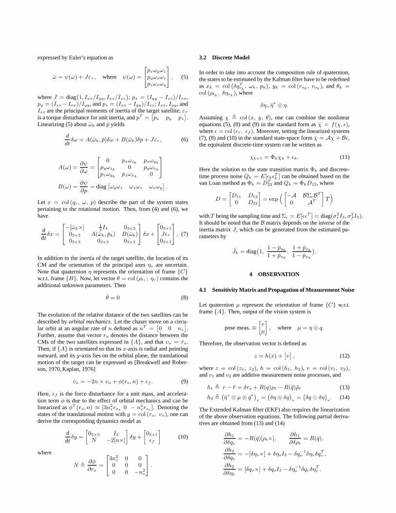
unit delay

ICP

point cloud

Vision sys.

pose

initial guess

(a) ICP takes initial guess from the last pose estimate

EKFICP

pose

initial guess

(b) ICP and EKF in closed-loop

Figure 2: Different configurations for tracking a moving object.

?

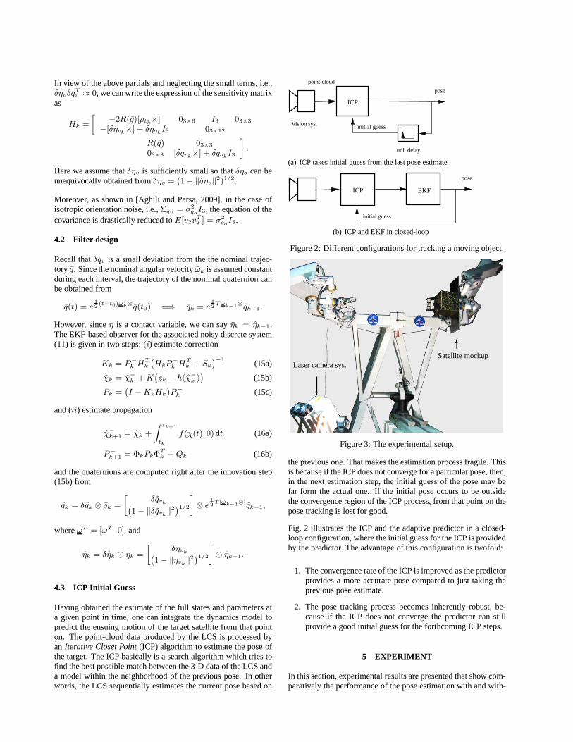
Laser camera sys.

6Satellite mockup

Figure 3: The experimental setup.

the previous one. That makes the estimation process fragile. Thisis because if the ICP does not converge for a particular pose,then,in the next estimation step, the initial guess of the pose maybefar form the actual one. If the initial pose occurs to be outsidethe convergence region of the ICP process, from that point onthepose tracking is lost for good.

Fig. 2 illustrates the ICP and the adaptive predictor in a closed-loop configuration, where the initial guess for the ICP is providedby the predictor. The advantage of this configuration is twofold:

1. The convergence rate of the ICP is improved as the predictorprovides a more accurate pose compared to just taking theprevious pose estimate.

2. The pose tracking process becomes inherently robust, be-cause if the ICP does not converge the predictor can stillprovide a good initial guess for the forthcoming ICP steps.

5 EXPERIMENT

In this section, experimental results are presented that show com-paratively the performance of the pose estimation with and with-

(a) The satellite CAD model.

−0.4

−0.3

−0.2

−0.1

0

0.1

0.2

0.3

0.4 −0.4−0.3

−0.2−0.1

00.1

0.20.3

0.4

−2.8−2.6−2.4−2.2

−2

X (m)Y (m)

Z(m

)

(b) The point-cloud data from scanning of the satellite.

Figure 4: Matching points from the CAD model and the scanneddata to estimate the satellite pose.

out KF in the loop.

Fig. 3 illustrates the experimental setup where a satellitemockupis attached to a manipulator arm, which is driven by a simula-tor according to orbital dynamics. The Neptec’s Laser Cam-era System (LCS) [Samson et al., 2004], is used to obtain thepose measurements at a rate of 2 Hz. For the spacecraft simu-lator that drives the manipulator, parameters are selectedasI =diag

[

4 8 5]

kgm2 andρTt =

[

−0.15 0 0]

m. The solidmodel of the satellite mockup, Fig. 4(a), and the point-cloud data,generated by the laser camera system, Fig. 4(b), are used by theICP algorithm to estimate the satellite pose according to the twoschemes for providing the initial guess as shown in Fig. 2.

The robustness of the pose estimation of the moving satellite withand without incorporating the KF are illustrated in Figs 5 and 6,respectively. It is evident from Figs. 5(a) and 5(b) that theICP-based pose estimation is fragile if the initial guess is taken fromthe last estimated pose. This will cause growing ICP fit metricover time, as shown in Fig. 5(c), that eventually lead to a totalfailure at t = 90 sec. On the other hand, the pose estimationwith ICP and the KF in the closed loop configuration exhibitsrobustness as shown in Figs. 6(a) and 6(b). Trajectories of the es-timated angular velocities obtained from the KF versus the actualtrajectories calculated by using the manipulator kinematics are il-lustrated in Fig. 7. The plot shows that the estimator converges ataroundt = 15 sec.

0 20 40 60 80 100 1200.8

0.9

1

0 20 40 60 80 100 1200.34

0.36

0.38

0 20 40 60 80 100 120−0.05

0

0.05

0.1

Time (s)

r x(m

)r y

(m)

r z(m

)

(a) Position trajectories

0 20 40 60 80 100 120−200

0

200

0 20 40 60 80 100 120

0

20

40

0 20 40 60 80 100 120−100

−80

−60

−40

−20

Time (s)

α(d

eg)

β(d

eg)

γ(d

eg)

(b) Euler angles

0 20 40 60 80 100 1200

0.1

0.2

Time (s)

erro

r

(c) Normalized ICP fit metric

Figure 5: Pose estimation without incorporating EKF

6 CONCLUSION

A method for pose estimation of free-floating space objects byincorporating a dynamic estimator in the ICP algorithm has beenpresented. An adaptive extended Kalman filter was used for es-timating the relative pose of two free-falling satellites that movein close orbits near each other using position and orientation dataprovided by a laser vision system. Not only does the filter esti-mate the system states, but also all the dynamics parametersofthe target. Experimental results obtained from scanning a mov-ing satellite mockup demonstrated that the pose tracking based onICP alone was fragile and did not converge. On the other hand,the integration scheme of the KF and ICP yielded a robust posetracking.

0 20 40 60 80 100 1200.8

0.85

0.9

0 20 40 60 80 100 1200.34

0.35

0.36

0.37

0 20 40 60 80 100 120−0.05

0

0.05

0.1

Time

r x(m

)r y

(m)

r z(m

)

EKFICP

(a) Position trajectories

0 20 40 60 80 100 120−200

0

200

0 20 40 60 80 100 120

0

20

40

0 20 40 60 80 100 120−100

−80

−60

α(d

eg)

β(d

eg)

γ(d

eg) EKF

ICP

(b) Euler angles

0 20 40 60 80 100 1200

0.05

Time (s)

erro

r

(c) Normalized ICP fit metric

Figure 6: Pose estimation with the closed loop ICP-EKF

REFERENCES

Aghili, F. and Parsa, K., 2009. Motion and parameter estima-tion of space objetcs using laser-vision data. AIAA JournalofGuidance, Control, and Dynamics 32(2), pp. 537–459.

Amor, B. B., Ardabilian, M. and Chen, L., 2006. New ex-periments on icp-based 3d face recognition and authentication.In: IEEE Int. Conference on Pattern Recofgnition, Hong Kong,pp. 1195–1199.

Besl, P. J. and McKay, N. D., 1992. A method for registration of3-d shapes. IEEE Trans. on Pattern Analysis & Machine Intelli-gence 14(2), pp. 239–256.

0 20 40 60 80 100 120

−0.06

−0.04

−0.02

0

0.02

0 20 40 60 80 100 1200

0.1

0.2

0 20 40 60 80 100 120

0

0.05

0.1

Time (s)

ActualEKF

ωx

(rad

/s)

ωy

(rad

/s)

ωz

(rad

/s)

Figure 7: Angular velocities

Breakwell, J. and Roberson, R., 1970. Oribtal and attitude dy-namics. Lecture notes.

Faugeras, O. D. and Herbert, M., 1986. The representation,recognition, and locating of 3-d objects. The International Jour-nal of Robotics Research 5(3), pp. 27–52.

Kaplan, M. H., 1976. Modern Spacecraft Dynamics and Control.Wiley, New York.

Lefferts, E. J., Markley, F. L. and Shuster, M. D., 1982. Kalmanfiltering for spacecraft attitude estimation. Journal of Guidance5(5), pp. 417–429.

Lichter, M. D. and Dubowsky, S., 2004. State, shape, and param-eter esitmation of space object from range images. In: IEEE Int.Conf. On Robotics & Automation, New Orleans, pp. 2974–2979.

Masutani, Y., Iwatsu, T. and Miyazaki, F., 1994. Motion estima-tion of unknown rigid body under no external forces and mo-ments. In: IEEE Int. Conf. on Robotics & Automation, SanDiego, pp. 1066–1072.

Rekleitis, I., Martin, E., Rouleau, G., L’Archeveque, R.,Parsa, K.and Dupuis, E., 2007. Autonomous capture of a tumbling satel-lite. Journal of Field Robotics, Special Issue on Space Robotics24(4), pp. 275–296.

Samson, C., English, C., Deslauriers, A., Christie, I., Blais, F.and Ferrie, F., 2004. Neptec 3D laser camera system: From spacemision STS-105 to terrestrial applications. Canadian Aeronauticsand Space Journal 50(2), pp. 115–123.

Simon, D. A., Herbert, M. and Kanade, T., 1994. Real-time 3-destimation using a high-speed range sensor. In: IEEE Int. Confer-ence on Robotics & Automation, San Diego, CA, pp. 2235–2241.

Yoshida, K., 2003. Engineering test satellite VII flight experimentfor space robot dynamics and control: Theories on laboratory testbeds ten years ago, now in orbit. The Int. Journal of RoborticsResearch 22(5), pp. 321–335.

Zimpfer, D. and Spehar, P., 1996. STS-71 Shuttle/MIR GNC mis-sion overview. In: Advances in Astronautical Sciences, AmericanAstronautical Society, San Diego, CA, pp. 441–460.