Submission to the IJCV Special Issue on Learning for Vision and Vision for Learning, Sept. 2005, 2nd revised version Aug. 2007.

Robust Object Detection with InterleavedCategorization and Segmentation

Bastian Leibe1, Ales Leonardis2, and Bernt Schiele3

Abstract— This paper presents a novel method for detectingand localizing objects of a visual category in cluttered real-worldscenes. Our approach considers object categorization and figure-ground segmentation as two interleaved processes that closelycollaborate towards a common goal. As shown in our work, thetight coupling between those two processes allows them to benefitfrom each other and improve the combined performance.

The core part of our approach is a highly flexible learned rep-resentation for object shape that can combine the information ob-served on different training examples in a probabilistic extensionof the Generalized Hough Transform. The resulting approach candetect categorical objects in novel images and automatically infera probabilistic segmentation from the recognition result. Thissegmentation is then in turn used to again improve recognitionby allowing the system to focus its efforts on object pixels and todiscard misleading influences from the background. Moreover,the information from where in the image a hypothesis draws itssupport is employed in an MDL based hypothesis verificationstage to resolve ambiguities between overlapping hypotheses andfactor out the effects of partial occlusion.

An extensive evaluation on several large data sets shows thatthe proposed system is applicable to a range of different objectcategories, including both rigid and articulated objects. In ad-dition, its flexible representation allows it to achieve competitiveobject detection performance already from training sets that arebetween one and two orders of magnitude smaller than thoseused in comparable systems.

Index Terms— object categorization, object detection, segmen-tation, clustering, Hough transform, hypothesis selection, MDL

I. INTRODUCTION

Object recognition has reached a level where current ap-proaches can identify a large number of previously seen andknown objects. However, the more general task of objectcategorization, that is of recognizing unseen-before objectsof a given category and assigning the correct category label,is still less well-understood. Obviously, this task is moredifficult, since it requires a method to cope with large within-class variations of object colors, textures, and shapes, whileretaining at the same time enough specificity to avoid mis-classifications. This is especially true for object detection incluttered real-world scenes, where objects are often partiallyoccluded and where similar-looking background structures canact as additional distractors. Here, it is not only necessary toassign the correct category label to an image, but also to find

1Computer Vision Laboratory, ETH Zurich, Switzerland, email:leibe@vision.ee.ethz.ch

2Faculty of Computer and Information Science, University of Ljubljana,Slovenia, email: alesl@fri.uni-lj.si

3Department of Computer Science, TU Darmstadt, Germany, email:schiele@informatik.tu-darmstadt.de

the objects in the first place and to separate them from thebackground.

Historically, this step of figure-ground segmentation haslong been seen as an important and even necessary precursorfor object recognition [45]. In this context, segmentation ismostly defined as a data driven, that is bottom-up, process.However, except for cases where additional cues such asmotion or stereo could be used, purely bottom-up approacheshave so far been unable to yield figure-ground segmentationsof sufficient quality for object categorization. This is also dueto the fact that the notion and definition of what constitutes anobject is largely task-specific and cannot be answered in an un-informed way. The general failure to achieve task-independentsegmentation, together with the success of appearance-basedmethods to provide recognition results without prior segmenta-tion, has led to the separation of the two areas and the furtherdevelopment of recognition independent from segmentation.It has been argued, however, both in computer vision [2]and in human vision [57], [74], [53] that recognition andsegmentation are heavily intertwined processes and that top-down knowledge from object recognition can and should beused for guiding the segmentation process.

In our work, we follow this inspiration by addressing objectdetection and segmentation not as separate entities, but astwo closely collaborating processes. In particular, we presenta local-feature based approach that combines both capabilitiesinto a common probabilistic framework. As our experimentswill show, the use of top-down segmentation improves therecognition results considerably.

In order to learn the appearance variability of an objectcategory, we first build up a codebook of local appearances thatare characteristic for (a particular viewpoint of) its memberobjects. This is done by extracting local features aroundinterest points and grouping them with an agglomerativeclustering scheme. As this initial clustering step will be appliedto large data sets, an efficient implementation is crucial. Wetherefore evaluate different clustering methods and describean efficient algorithm that can be used for the codebookgeneration process.

Based on this codebook, we then learn an Implicit ShapeModel (ISM) that specifies where on the object the codebookentries may occur. As the name already suggests, we donot try to define an explicit model for all possible shapes aclass object may take, but instead define “allowed” shapesimplicitly in terms of which local appearances are consistentwith each other. The advantages of this approach are its greaterflexibility and the smaller number of training examples itneeds to see in order to learn possible object shapes. For

1

2

example, when learning to categorize articulated objects suchas cows or pedestrians, our method does not need to seeevery possible articulation in the training set. It can combinethe information of a front leg seen on one training instancewith the information of a rear leg from a different instanceto recognize a test image with a novel articulation, since bothleg positions are consistent with the same object hypothesis.This idea is similar in spirit to approaches that representnovel objects by a combination of class prototypes [30], orof familiar object views [72]. However, the main differenceof our approach is that here the combination does not occurbetween entire exemplar objects, but through the use of localimage features, which again allows a greater flexibility.

Directly connected to the recognition procedure, we derive aprobabilistic formulation for the top-down segmentation prob-lem, which integrates learned knowledge of the recognizedcategory with the supporting information in the image. Theresulting procedure yields a pixel-wise figure-ground segmen-tation as a result and extension of recognition. In addition, itdelivers a per-pixel confidence estimate specifying how muchthis segmentation can be trusted.

The automatically computed top-down segmentation is thenin turn used to improve recognition. First, it allows to only ag-gregate evidence over the object region and discard influencesfrom the background. Second, the information from where inthe image a hypothesis draws its support makes it possibleto resolve ambiguities between overlapping hypotheses. Weformalize this idea in a criterion based on the MinimumDescription Length (MDL) principle. The resulting procedureconstitutes a novel mechanism that allows to analyze scenescontaining multiple objects in a principled manner. The wholeapproach is formulated in a scale-invariant manner, making itapplicable in real-world situations where the object scale isoften unknown.

We experimentally evaluate the different components of ouralgorithm and quantify the robustness of the resulting approachto object detection in cluttered real-world scenes. Our resultsshow that the proposed scheme achieves good detection resultsfor both rigid and articulated object categories while beingrobust to large scale changes.

This paper is structured as follows. The next sectiondiscusses related work. After that, Section III introducesour underlying codebook representation. The following threesections then present the main steps of the ISM approachfor recognition (Sec. IV), top-down segmentation (Sec. V),and segmentation-based verification (Sec. VI). Section VIIexperimentally evaluates the different stages of the systemand applies it to several challenging multi-scale test sets ofdifferent object categories, including cars, motorbikes, cows,and pedestrians. A final discussion concludes our work.

II. RELATED WORK

In the following, we give an overview of current approachesto object detection and categorization, with a focus on thestructural representations they employ. In addition, we doc-ument the recent transition from recognition to top-downsegmentation, which has been developing into an area of activeresearch.

A. Structure Representations for Object Categorization

A large class of methods match object structure by com-puting a cost term for the deformation needed to transforma prototypical object model to correspond with the image.Prominent examples of this approach include Deformable Tem-plates [81], [63], Morphable Models [31], or Shape ContextMatching [4]. The main difference between them lies in theway point correspondences are found and in the choice ofenergy function for computing the deformation cost (e.g. Eu-clidean distances, strain energy, thin plate splines, etc.). Cooteset al. [14] extend this idea and characterize objects by meansand modes of variation for both shape and texture. Their ActiveAppearance Models first warp the object to a mean shape andthen estimate the combined modes of variation of the concate-nated shape and texture models. For matching the resultingAAMs to a test image, they learn the relationship betweenmodel parameter displacements and the induced differencesin the reconstructed model image. Provided that the methodis initialized with a close estimate of the object’s position andsize, a good overall match to the object is typically obtainedin a few iterations, even for deformable objects.

Wiskott et al. [78] propose a different structural modelknown as Bunch Graph. The original version of this ap-proach represents object structure as a graph of hand-definedlocations, at which local jets (multidimensional vectors ofsimple filter responses) are computed. The method learnsan object model by storing, for each graph node, the set(“bunch”) of all jet responses that have been observed in thislocation on a hand-aligned training set. During recognition,only the strongest response is taken per location, and the jointmodel fit is optimized by an iterative elastic graph matchingtechnique. This approach has achieved impressive results forface identification tasks, but an application to more objectclasses is made difficult by the need to model a set of suitablegraph locations.

In contrast to those deformable representations, most clas-sic object detection methods either use a monolithic objectrepresentation [59], [56], [15] or look for local features infixed configurations [62], [75]. Schneiderman & Kanade [62]express the likelihood of object and non-object appearanceusing a product of localized histograms, which represent thejoint statistics of subsets of wavelet coefficients and theirposition on the object. The detection decision is made by alikelihood-ratio classifier. Multiple detectors, each specializedto a certain orientation of the object, are used to achieve recog-nition over a variety of poses, including frontal and profilefaces and various views of passenger cars. Their approachachieves very good detection results on standard databases,but is computationally still relatively costly. Viola & Jones[75] instead focus on building a speed-optimized system forface detection by learning a cascade of simple classifiers basedon Haar wavelets. In recent years, this class of approacheshas been shown to yield fast and accurate object detectionresults under real-world conditions [69]. However, a drawbackof these methods is that since they do not explicitly modellocal variations in object structure (e.g. from body parts indifferent articulations), they typically need a large number of

3

training examples in order to learn the allowed changes inglobal appearance.

One way to model these local variations is by representingobjects as an assembly of parts. Mohan et al. [51] use a setof hand-defined appearance parts, but learn an SVM-basedconfiguration classifier for pedestrian detection. The resultingsystem performs significantly better than the original full-body person detector by [56]. In addition, its component-basedarchitecture makes it more robust to partial occlusion. Heiseleet al. [28] use a similar approach for component-based facedetection. As an extension of Mohan et al.’s approach, theirmethod also includes an automatic learning step for findinga set of discriminative components from user-specified seedpoints. More recently, several other part-classifier approacheshave been proposed for pedestrian detection [58], [47], [79],also based on manually specified parts.

Burl et al. [9] learn the assembly of hand-selected (appear-ance) object parts by modeling their joint spatial probabilitydistribution. Weber et al. [77] build on the same framework,but also learn the local parts and estimate their joint dis-tribution. Fergus et al. [23] extend this approach to scale-invariant object parts and estimate their joint spatial andappearance distribution. The resulting Constellation Model hasbeen successfully demonstrated on several object categories.In its original form, it modeled the relative part locationsby a fully connected graph. However, the complexity of thecombined estimation step restricted this model to a relativelysmall number of (only 5–6) parts. In later versions, Ferguset al. [22] therefore replaced the fully-connected graph by asimpler star topology, which can handle a far larger numberof parts using efficient inference algorithms [21].

Agarwal & Roth [1] keep a larger number of object partsand apply a feature-efficient classifier for learning spatialconfigurations between pairs of parts. However, their learningapproach relies on the repeated observation of cooccurrencesbetween the same parts in similar spatial relations, whichagain requires a large number of training examples. Ullmanet al. [73] represent objects by a set of fragments that werechosen to maximize the information content with respect toan object class. Candidate fragments are extracted at differentsizes and from different locations of an initial set of trainingimages. From this set, their approach iteratively selects thosefragments that add the maximal amount of information aboutthe object class to the already selected set, thus effectivelyresulting in a cover of the object. In addition, the approachautomatically selects, for each fragment, the optimal thresholdsuch that it can be reliably detected. For recognition, however,only the information which model fragments were detected isencoded in a binary-valued feature vector (similar to Agarwal& Roth’s), onto which a simple linear classifier is appliedwithout any additional shape model. The main challenge forthis approach is that the complexity of the fragment selectionprocess restricts the method to very low image resolutions(e.g. 14 × 21 pixels), which limits its applicability in practice.

Robustness to scale changes is one of the most importantproperties of any recognition system that shall be appliedin real-world situations. Even when the camera location isrelatively fixed, objects of interest may still exhibit scale

changes of at least a factor of two, simply because they occurat different distances to the camera. It is therefore necessarythat the recognition mechanism itself can compensate for acertain degree of scale variation. Many current object detec-tion methods deal with the scale problem by performing anexhaustive search over all possible object positions and scales[56], [62], [75], [47], [15], [79]. This exhaustive search im-poses severe constraints, both on the detector’s computationalcomplexity and on its discriminance, since a large numberof potential false positives need to be excluded. An oppositeapproach is to let the search be guided by image structuresthat give cues about the object scale. In such a system, aninitial interest point detector tries to find structures whoseextent can be reliably estimated under scale changes. Thesestructures are then combined to derive a comparatively smallnumber of hypotheses for object locations and scales. Onlythose hypotheses that pass an initial plausibility test need to beexamined in detail. In recent years, a range of scale-invariantinterest point detectors have become available which can beused for this purpose [39], [40], [50], [32], [71], [46].

In our approach, we combine several of the above ideas.Our system uses a large number of automatically selectedparts, based on the output of an interest point operator, andcombines them flexibly in a star topology. Robustness toscale changes is achieved by employing scale-invariant interestpoints and explicitly incorporating the scale dimension in thehypothesis search procedure. The whole approach is optimizedfor efficient learning and accurate detection from small trainingsets.

B. From Recognition to Top-Down Segmentation

The traditional view of object recognition has been thatprior to the recognition process, an earlier stage of perceptualorganization occurs to determine which features, locations,or surfaces most likely belong together [45]. As a result,the segregation of the image into a figure and a groundpart has often been seen as a prerequisite for recognition. Inthat context, segmentation is mostly defined as a bottom-upprocess, employing no higher-level knowledge. State-of-the-art segmentation methods combine grouping of similar imageregions with splitting processes concerned with finding mostlikely borders [66], [65], [44]. However, grouping is mostlydone based on low-level image features, such as color ortexture statistics, which require no prior knowledge. Whilethat makes them universally applicable, it often leads topoor segmentations of objects of interest, splitting them intomultiple regions or merging them with parts of the background[7].

Results from human vision indicate, however, that objectrecognition processes can operate before or intertwined withfigure-ground organization and can in fact be used to drivethe process [57], [74], [53]. In consequence, the idea to useobject-specific information for driving figure-ground segmen-tation has recently developed into an area of active research.Approaches, such as Deformable Templates [81], or ActiveAppearance Models [14] are typically used when the objectof interest is known to be present in the image and an initial

4

estimate of its size and location can be obtained. Examplesof successful applications include tracking and medical imageanalysis.

Borenstein & Ullman [7] represent object knowledge usingimage fragments together with their figure-ground labeling (aslearned from a training set). Class-specific segmentations areobtained by fitting fragments to the image and combiningthem in jigsaw-puzzle fashion, such that their figure-groundlabels form a consistent mapping. While the authors presentimpressive results for segmenting side views of horses, theirinitial approach includes no global recognition process. Asonly the local consistency of adjacent pairs of fragmentsis checked, there is no guarantee that the resulting coverreally corresponds to an object and is not just caused bybackground clutter resembling random object parts. In morerecent work, the approach is extended to also combine thetop-down segmentation with bottom-up segmentation cues inorder to obtain higher-quality results [6].

Tu et al. [70] have proposed a system that integrates faceand text detection with region-based segmentation of the fullimage. However, their focus is on segmenting images intomeaningful regions, not on separating objects of interest fromthe background.

Yu & Shi [80] and Ferrari et al. [24] both present parallelsegmentation and recognition systems. Yu & Shi formulatethe segmentation problem in a graph theoretic framework thatcombines patch and pixel groupings, where the final solutionis found using the Normalized Cuts criterion [66]. Ferrari etal. start from a small set of initial matches and then employan iterative image exploration process that grows the matchingregion by searching for additional correspondences and seg-menting the object in the process. Both methods achieve goodsegmentation results in cluttered real-world settings. However,both systems need to know the exact objects beforehand inorder to extract their most discriminant features or search foradditional correspondences.

In our application, we cannot assume the objects to beknown beforehand — only familiarity with the object categoryis required. This means that the system needs to have seensome examples of the object category before, but those do nothave to be the ones that are to be recognized later. Obviously,this makes the task more difficult, since we cannot rely onany object-specific feature, but have to compensate for largeintra-class variations.

III. CODEBOOK REPRESENTATIONS

The first task of any local-feature based approach is to deter-mine which features in the image correspond to which objectstructures. This is generally known as the correspondenceproblem. For detecting and identifying known objects, thistranslates to the problem of robustly finding exactly the samestructures again in new images under varying imaging con-ditions [61], [41], [24].As the ideal appearance of the modelobject is known, the extracted features can be very specific.In addition, the objects considered by those approaches areoften rigid, so that the relative feature configuration stays thesame for different images. Thus, a small number of matches

typically suffices to estimate the object pose, which can thenin turn be used to actively search for new matches thatconsolidate the hypothesis [41], [24].

When trying to find objects of a certain category, however,the task becomes more difficult. Not only is the featureappearance influenced by different viewing conditions, butboth the object composition (i.e. which local structures arepresent on the object) and the spatial configuration of featuresmay also vary considerably between category members. Ingeneral, only very few local features are present on all categorymembers. Hence, it is necessary to employ a more flexiblerepresentation.

In this section, we introduce the first level of such arepresentation. As basis, we use an idea inspired by the workof [9], [77], and [1]. We build up a vocabulary (in the followingtermed a codebook) of local appearances that are characteristicfor a certain viewpoint of an object category by sampling localfeatures that repeatedly occur on a set of training images ofthis category. Features that are visually similar are groupedtogether in an unsupervised clustering step. The result isa compact representation of object appearance in terms ofwhich novel images can be expressed. When pursuing suchan approach, however, it is important to represent uncertaintyon all levels: while matching the unknown image content tothe known codebook representation; and while accumulatingthe evidence of multiple such matches, e.g. for inferring thepresence of the object.

Codebook representations have become a popular tool forobject categorization recently, and many approaches use vari-ations of this theme [9], [77], [23], [38], [1], [7], [73], [21].However, there are still large differences in how the groupingstep is performed, how the matching uncertainty is represented,and how the codebook is later used for recognition. In thefollowing, we describe our codebook generation procedureand review two popular methods for achieving the groupingstep, namely k-means and agglomerative clustering. As thelatter usually scales poorly to large data sets, we present anefficient average-link clustering algorithm which runs at thesame time and space complexity as k-means. This algorithm isnot based on an approximation, but computes the exact result,thus making it possible to use agglomerative clustering also forlarge-scale codebook generation. After the remaining stagesof our recognition method have been introduced, Section VII-C will then present an experimental comparison of the twoclustering methods in the context of a recognition task.

A. Codebook Generation

We start by applying a scale-invariant interest point detectorto obtain a set of informative regions for each image. Byextracting features only from those regions, the amount ofdata to be processed is reduced, while the interest point detec-tor’s preference for certain structures assures that “similar”regions are sampled on different objects. Several differentinterest point detectors are available for this purpose. In thispaper, we use and evaluate Harris [27], Harris-Laplace [50],Hessian-Laplace [50], and Difference-of-Gaussian (DoG) [40]detectors. We then represent the extracted image regions by a

5

Fig. 1. Local information used in the codebook generation process: (left)interest points; (right) features extracted around the interest points (visualizedby the corresponding image patches). In most of our experiments, between 50and 200 features are extracted per object.

local descriptor. Again, several descriptor choices are availablefor this step. In this paper, we compare simple GreyvaluePatches [1], SIFT [40], and Local Shape Context [4], [49]descriptors. In order to develop the different stages of ourapproach, we will abstract from the concrete choice of regiondetector and descriptor and simply refer to the extracted localinformation by the term feature. Sections VII-E and VII-Fwill then systematically evaluate the different choices for thedetectors and descriptors. Figure 1 shows the extracted featuresfor two example images (in this case using Harris interestpoints). As can be seen from those examples, the sampledinformation provides a dense cover of the object, leaving outonly uniform regions. This process is repeated for all trainingimages, and the extracted features are collected.

Next, we group visually similar features to create a code-book of prototypical local appearances. In order to keep therepresentation as simple as possible, we represent all featuresin a cluster by their mean, the cluster center. Of course, anecessary condition for this is that the cluster center is ameaningful representative for the whole cluster. In that respect,it becomes evident that the goal of the grouping stage mustnot be to obtain the smallest possible number of clusters,but to ensure that the resulting clusters are visually compactand contain the same kind of structure. This is an importantconsideration to bear in mind when choosing the clusteringmethod.

B. Clustering Methods

1) K-means Clustering: The k-means algorithm [42] is oneof the simplest and most popular clustering methods. It pursuesa greedy hill-climbing strategy in order to find a partition ofthe data points that optimizes a squared-error criterion. Thealgorithm is initialized by randomly choosing k seed pointsfor the clusters. In all following iterations, each data pointis assigned to the closest cluster center. When all points havebeen assigned, the cluster centers are recomputed as the meansof all associated data points. In practice, this process convergesto a local optimum within few iterations.

Many approaches employ k-means clustering because ofits computational simplicity, which allows to apply it to verylarge data sets [77]. Its time complexity is O(Nk�d), where

N is the number of data points of dimensionality d; k is thedesired number of clusters; and � is the number of iterationsuntil the process converges. However, k-means clustering hasseveral known deficiencies. Firstly, it requires the user tospecify the number of clusters in advance. Secondly, there isno guarantee that the obtained clusters are visually compact.Because of the fixed value of k, some cluster centers maylie in-between several “real” clusters, so that the mean imageis not representative of all grouped patches. Thirdly, k-meansclustering is only efficient for small values of k; when appliedto our task of finding a large number (k ≈ N

10 ) of visuallycompact clusters, its asymptotic run-time becomes quadratic.Last but not least, the k-means procedure is only guaranteedto find a local optimum, so the results may be quite differentfrom run to run.

2) Agglomerative Clustering: Other approaches thereforeuse agglomerative clustering schemes, which automaticallydetermine the number of clusters by successively mergingfeatures until a cut-off threshold t on the cluster compactness isreached [1], [34]. However, both the runtime and the memoryrequirements are often significantly higher for agglomerativemethods. Especially the memory requirements impose a prac-tical limit. The standard average-link algorithm, as found inmost textbooks, requires an O(N 2) similarity matrix to bestored. In practice, this means that the algorithm is onlysuitable for up to 15–25,000 input points on today’s machines.After that, its space requirements outgrow the size of theavailable main memory, and the algorithm incurs detrimentalpage swapping costs.

Given the large amounts of data that need to be processed,an efficient implementation of the clustering algorithm istherefore not only a nice extension, but indeed crucial for itsapplicability. Fortunately, it turns out that for special choicesof the clustering criterion and similarity measure, including theones we are using, a more efficient algorithm is available thatruns in O(N 2d) and needs only O(N) space. Although thebasic components of this algorithm are already more than 25years old, it has so far been little known in the ComputerVision community. The following section will describe itsderivation in more detail.

C. RNN Algorithm for Agglomerative Clustering

The main complexity of the standard average-link algorithmcomes from the effort to ensure that clusters are merged in theright order. The improvement presented in this section is dueto the insight by de Rham [17] and Benzecri [5] that for someclustering criteria, the same results can be achieved also whenspecific clusters are merged in a different order.

The algorithm is based on the construction of reciprocalnearest neighbor pairs (RNN pairs), that is of pairs of pointsa and b, such that a is b’s nearest neighbor and vice versa[17], [5]. It is applicable to clustering criteria that fulfillBruynooghe’s reducibility property [8]. This criterion demandsthat when two clusters ci and cj are agglomerated, the simi-larity of the merged cluster to any third cluster ck may only

6

Algorithm 1 The RNN algorithm for Average-Link clusteringwith nearest-neighbor chains.

// Start the chain L with a random point v ∈ V .// All remaining points are kept in R.last ← 0; lastsim[0] ← 0L[last ] ← v ∈ V; R ← V\v (1)

while R �= ∅ do// Search for the next NN in R and retrieve its similarity sim.(s, sim) ← getNearestNeighbor(L[last ], R) (2)

if sim > lastsim[last] then// No RNNs → Add s to the NN chainlast ← last + 1L[last ] ← s; R ← R\{s}lastsim[last ] ← sim (3)

else// Found RNNs → agglomerate the last two chain linksif lastsim[last ] > t then

s ← agglomerate(L[last ], L[last − 1])R ← R∪ {s}last ← last − 2 (4)

else// Discard the current chain.last ← −1

end ifend if

if last < 0 then// Initialize a new chain with another random point v ∈ R.last ← last + 1L[last ] ← v ∈ R; R ← R\{v} (5)

end ifend while

decrease, compared to the state before the merging action:

sim(ci, cj) ≥ sup(sim(ci, ck), sim(cj , ck)) ⇒sup(sim(ci, ck), sim(cj , ck)) ≥ sim(ci ∪ cj , ck). (1)

The reducibility property has the effect that the agglomerationof a reciprocal nearest-neighbor pair does not alter the nearest-neighbor relations of any other cluster. It is easy to see thatthis property is fulfilled, among others, for the group averagecriterion (regardless of the employed similarity measure) andthe centroid criterion based on correlation (though not onEuclidean distances). Let X =

{x(1), . . . , x(N)

}and Y ={

y(1), . . . , y(M)}

be two clusters. Then those criteria aredefined as

group avg.: sim(X, Y ) =1

NM

N∑i=1

M∑j=1

sim(x(i), y(j)), (2)

centroid: sim(X, Y ) = sim

⎛⎝1N

N∑i=1

x(i),1M

M∑j=1

y(j)

⎞⎠. (3)

As soon as an RNN pair is found, it can be agglomerated (acomplete proof that this results in the correct clustering can befound in [5]). The key to an efficient implementation is thusto ensure that RNNs can be found with as little recomputationas possible.

This can be achieved by building a nearest-neighbor chain[5]. An NN-chain consists of an arbitrary point, followed by

its nearest neighbor, which is again followed by its nearestneighbor from among the remaining points, and so on. It iseasy to see that each NN-chain ends in an RNN pair. Thestrategy of the algorithm is thus to start with an arbitrarypoint (Alg. 1, step (1)) and build up an NN-chain (2,3). Assoon as an RNN pair is found, the corresponding clustersare merged if their similarity is above the cut-off thresholdt; else the current chain is discarded (4). The reducibilityproperty guarantees that when clusters are merged this way,the nearest-neighbor assignments stay valid for the remainingchain members, which can thus be reused for the next iteration.Whenever the current chain runs empty, a new chain is startedwith another random point (5). The resulting procedure issummarized in Algorithm 1.

An amortized analysis of this algorithm shows that a fullclustering requires at most 3(N − 1) iterations of the mainloop [5]. The run-time is thus bounded by the time requiredto search the nearest neighbors, which is in the simplest caseO(Nd). For low-dimensional data, this can be further reducedby employing efficient NN-search techniques.

When a new cluster is created by merging an RNN pair,its new similarity to other clusters needs to be recomputed.Applying an idea by [16], this can be done in O(N) space ifthe cluster similarity can be expressed in terms of centroids. Inthe following, we show that this is the case for group averagecriteria based on correlation or Euclidean distances.

Let 〈. . . 〉 denote the inner product of a pair of vectorsand µx, µy be the cluster means of X and Y . Then thegroup average clustering criterion based on correlation canbe reformulated as

sim(X, Y )=1

NM

N∑i=1

M∑j=1

〈x(i), y(j)〉 = 〈µx, µy〉, (4)

which follows directly from the linearity property of the innerproduct.

Let µx, µy and σ2x, σ2

y be the cluster means and variancesof X and Y . Then it can easily be verified that the groupaverage clustering criterion based on Euclidean distances canbe rewritten as

sim(X, Y ) = − 1NM

N∑i=1

M∑j=1

(x(i) − y(j))2

= −(σ2

x + σ2y + (µx − µy)2

)(5)

Using this formulation, the new distances can be obtainedin constant time, requiring just the storage of the mean andvariance for each cluster. Both the mean and variance of theupdated cluster can be computed incrementally:

µnew =Nµx + Mµy

N + M(6)

σ2new =

1N +M

(Nσ2

x + Mσ2y +

NM

N +M(µx − µy)2

)(7)

Taken together, these steps result in an average-link cluster-ing algorithm with O(N 2d) time and O(N) space complexity.Among some other criteria, this algorithm is applicable to thegroup average criterion with correlation or Euclidean distances

7

Appearance Codebook(Cluster Centers)

Spatial Occurrence Distributions(non-parametric)

LocalFeatures

Training Images(+Reference Segmentations)

x

y

sx

y

s

x

y

sx

y

s

…

…………

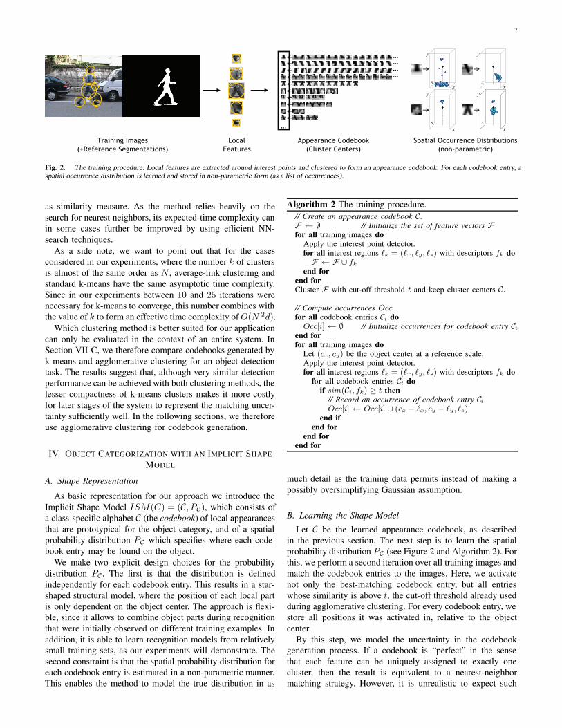
Fig. 2. The training procedure. Local features are extracted around interest points and clustered to form an appearance codebook. For each codebook entry, aspatial occurrence distribution is learned and stored in non-parametric form (as a list of occurrences).

as similarity measure. As the method relies heavily on thesearch for nearest neighbors, its expected-time complexity canin some cases further be improved by using efficient NN-search techniques.

As a side note, we want to point out that for the casesconsidered in our experiments, where the number k of clustersis almost of the same order as N , average-link clustering andstandard k-means have the same asymptotic time complexity.Since in our experiments between 10 and 25 iterations werenecessary for k-means to converge, this number combines withthe value of k to form an effective time complexity of O(N 2d).

Which clustering method is better suited for our applicationcan only be evaluated in the context of an entire system. InSection VII-C, we therefore compare codebooks generated byk-means and agglomerative clustering for an object detectiontask. The results suggest that, although very similar detectionperformance can be achieved with both clustering methods, thelesser compactness of k-means clusters makes it more costlyfor later stages of the system to represent the matching uncer-tainty sufficiently well. In the following sections, we thereforeuse agglomerative clustering for codebook generation.

IV. OBJECT CATEGORIZATION WITH AN IMPLICIT SHAPE

MODEL

A. Shape Representation

As basic representation for our approach we introduce theImplicit Shape Model ISM(C) = (C, PC), which consists ofa class-specific alphabet C (the codebook) of local appearancesthat are prototypical for the object category, and of a spatialprobability distribution PC which specifies where each code-book entry may be found on the object.

We make two explicit design choices for the probabilitydistribution PC . The first is that the distribution is definedindependently for each codebook entry. This results in a star-shaped structural model, where the position of each local partis only dependent on the object center. The approach is flexi-ble, since it allows to combine object parts during recognitionthat were initially observed on different training examples. Inaddition, it is able to learn recognition models from relativelysmall training sets, as our experiments will demonstrate. Thesecond constraint is that the spatial probability distribution foreach codebook entry is estimated in a non-parametric manner.This enables the method to model the true distribution in as

Algorithm 2 The training procedure.// Create an appearance codebook C.F ← ∅ // Initialize the set of feature vectors Ffor all training images do

Apply the interest point detector.for all interest regions �k = (�x, �y, �s) with descriptors fk doF ← F ∪ fk

end forend forCluster F with cut-off threshold t and keep cluster centers C.

// Compute occurrences Occ.for all codebook entries Ci do

Occ[i] ← ∅ // Initialize occurrences for codebook entry Ciend forfor all training images do

Let (cx, cy) be the object center at a reference scale.Apply the interest point detector.for all interest regions �k = (�x, �y, �s) with descriptors fk do

for all codebook entries Ci doif sim(Ci, fk) ≥ t then

// Record an occurrence of codebook entry CiOcc[i] ← Occ[i] ∪ (cx − �x, cy − �y, �s)

end ifend for

end forend for

much detail as the training data permits instead of making apossibly oversimplifying Gaussian assumption.

B. Learning the Shape Model

Let C be the learned appearance codebook, as describedin the previous section. The next step is to learn the spatialprobability distribution PC (see Figure 2 and Algorithm 2). Forthis, we perform a second iteration over all training images andmatch the codebook entries to the images. Here, we activatenot only the best-matching codebook entry, but all entrieswhose similarity is above t, the cut-off threshold already usedduring agglomerative clustering. For every codebook entry, westore all positions it was activated in, relative to the objectcenter.

By this step, we model the uncertainty in the codebookgeneration process. If a codebook is “perfect” in the sensethat each feature can be uniquely assigned to exactly onecluster, then the result is equivalent to a nearest-neighbormatching strategy. However, it is unrealistic to expect such

8

Segmentation

Refined Hypotheses(optional)

BackprojectedHypotheses

Backprojectionof Maxima

3D Voting Space(continuous)

x

y

s

ProbabilisticVoting

Matched CodebookEntries

Interest PointsOriginal Image

Fig. 3. The recognition procedure. Local features are extracted around interest points and compared to the codebook. Matching patches then cast probabilisticvotes, which lead to object hypotheses that can optionally be later refined by sampling more features. Based on the backprojected hypotheses, we then compute acategory-specific segmentation.

clean data in practical applications. We therefore keep eachpossible assignment, but weight it with the probability that thisassignment is correct. It is easy to see that for similarity scoressmaller than t, the probability that this patch could have beenassigned to the cluster during the codebook generation processis zero; therefore we do not need to consider those matches.The stored occurrence locations, on the other hand, reflect thespatial distribution of a codebook entry over the object area ina non-parametric form. Algorithm 2 summarizes the trainingprocedure.

C. Recognition Approach

Figure 3 illustrates the following recognition procedure.Given a new test image, we again apply an interest pointdetector and extract features around the selected locations. Theextracted features are then matched to the codebook to activatecodebook entries using the same mechanism as describedabove. From the set of all those matches, we collect consistentconfigurations by performing a Generalized Hough Transform[29], [3], [40]. Each activated entry casts votes for possiblepositions of the object center according to the learned spatialdistribution PC . Consistent hypotheses are then searched aslocal maxima in the voting space. When pursuing such anapproach, it is important to avoid quantization artifacts. In con-trast to usual practice (e.g. [41]), we therefore do not discretizethe votes, but keep their original, continuous values. Maximain this continuous space can be accurately and efficientlyfound using Mean-Shift Mode Estimation [10], [12]. Once ahypothesis has been selected, all patches that contributed toit are collected (Fig. 3(bottom)), thereby visualizing what thesystem reacts to. As a result, we get a representation of theobject including a certain border area. This representation canoptionally be further refined by sampling more local features.The backprojected response will later serve as the basis forcomputing a category-specific segmentation, as described inSection V.

1) Probabilistic Hough Voting: In the following, we castthe voting procedure into a probabilistic framework [34], [33].Let f be our evidence, an extracted image feature observed

at location �. By matching it to the codebook, we obtain aset of valid interpretations Ci with probabilities p(Ci|f, �). Ifa codebook cluster matches, it casts votes for different objectpositions. That is, for every Ci, we can obtain votes for severalobject categories/viewpoints on and positions x, according tothe learned spatial distribution p(on, x|Ci, �). Formally, thiscan be expressed by the following marginalization:

p(on, x|f, �) =∑

i

p(on, x|f, Ci, �)p(Ci|f, �). (8)

Since we have replaced the unknown image feature by aknown interpretation, the first term can be treated as indepen-dent from f . In addition, we match patches to the codebookindependent of their location. The equation thus reduces to

p(on, x|f, �) =∑

i

p(on, x|Ci, �)p(Ci|f). (9)

=∑

i

p(x|on, Ci, �)p(on|Ci, �)p(Ci|f). (10)

The first term is the probabilistic Hough vote for an objectposition given its class label and the feature interpretation. Thesecond term specifies a confidence that the codebook clusteris really matched on the target category as opposed to thebackground. This can be used to include negative examples inthe training process. Finally, the third term reflects the qualityof the match between image feature and codebook cluster.

When casting votes for the object center, the object scaleis treated as a third dimension in the voting space [35]. If animage feature found at location (ximg , yimg, simg) matchesto a codebook entry that has been observed at position(xocc, yocc, socc) on a training image, it votes for the followingcoordinates:

xvote = ximg − xocc(simg/socc) (11)

yvote = yimg − yocc(simg/socc) (12)

svote = (simg/socc). (13)

Thus, the vote distribution p(x|on, Ci, �) is obtained by castinga vote for each stored observation from the learned occurrencedistribution PC . The ensemble of all such votes together is then

9

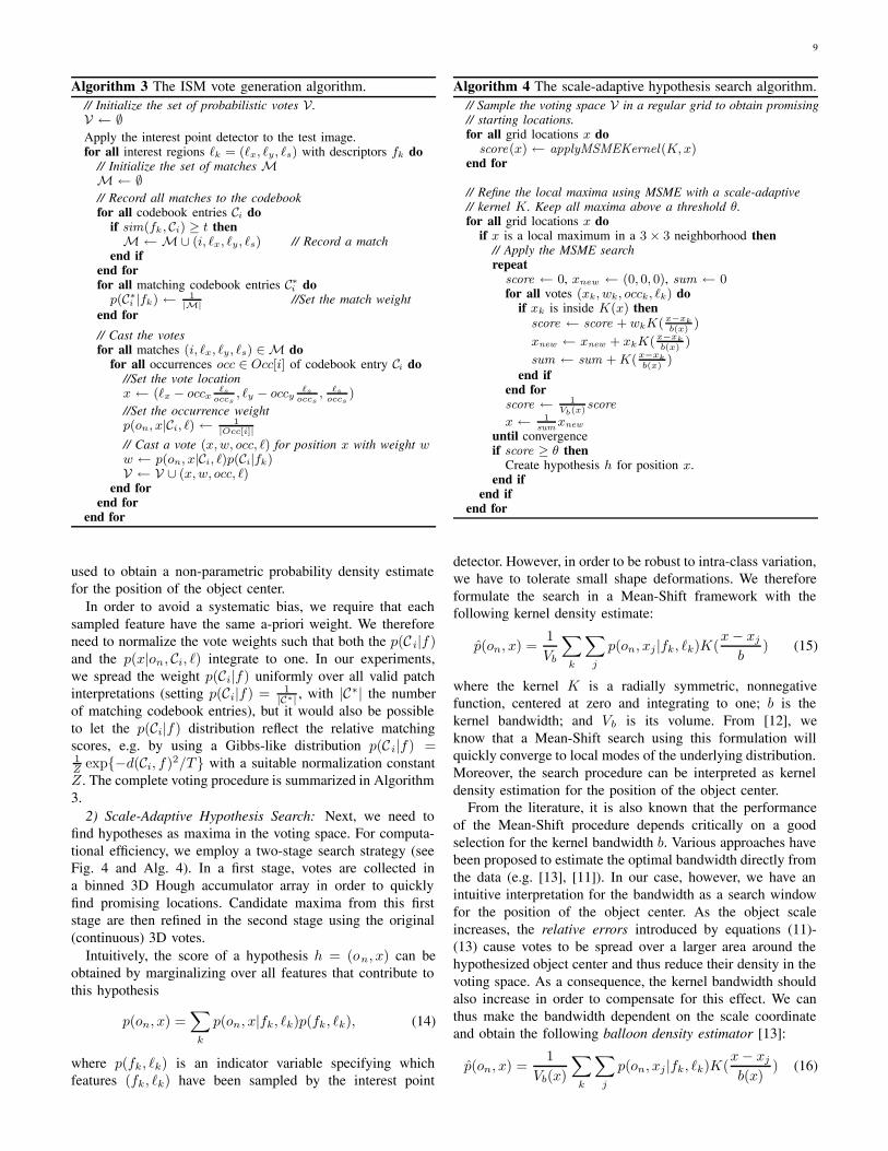
Algorithm 3 The ISM vote generation algorithm.// Initialize the set of probabilistic votes V .V ← ∅Apply the interest point detector to the test image.for all interest regions �k = (�x, �y, �s) with descriptors fk do

// Initialize the set of matches MM ← ∅// Record all matches to the codebookfor all codebook entries Ci do

if sim(fk, Ci) ≥ t thenM ←M∪ (i, �x, �y, �s) // Record a match

end ifend forfor all matching codebook entries C∗i do

p(C∗i |fk) ← 1|M| //Set the match weight

end for

// Cast the votesfor all matches (i, �x, �y, �s) ∈M do

for all occurrences occ ∈ Occ[i] of codebook entry Ci do//Set the vote locationx ← (�x − occx

�soccs

, �y − occy�s

occs, �s

occs)

//Set the occurrence weightp(on, x|Ci, �) ← 1

|Occ[i]|// Cast a vote (x,w, occ, �) for position x with weight ww ← p(on, x|Ci, �)p(Ci|fk)V ← V ∪ (x, w, occ, �)

end forend for

end for

used to obtain a non-parametric probability density estimatefor the position of the object center.

In order to avoid a systematic bias, we require that eachsampled feature have the same a-priori weight. We thereforeneed to normalize the vote weights such that both the p(C i|f)and the p(x|on, Ci, �) integrate to one. In our experiments,we spread the weight p(Ci|f) uniformly over all valid patchinterpretations (setting p(Ci|f) = 1

|C∗| , with |C∗| the numberof matching codebook entries), but it would also be possibleto let the p(Ci|f) distribution reflect the relative matchingscores, e.g. by using a Gibbs-like distribution p(C i|f) =1Z exp{−d(Ci, f)2/T } with a suitable normalization constantZ . The complete voting procedure is summarized in Algorithm3.

2) Scale-Adaptive Hypothesis Search: Next, we need tofind hypotheses as maxima in the voting space. For computa-tional efficiency, we employ a two-stage search strategy (seeFig. 4 and Alg. 4). In a first stage, votes are collected ina binned 3D Hough accumulator array in order to quicklyfind promising locations. Candidate maxima from this firststage are then refined in the second stage using the original(continuous) 3D votes.

Intuitively, the score of a hypothesis h = (on, x) can beobtained by marginalizing over all features that contribute tothis hypothesis

p(on, x) =∑

k

p(on, x|fk, �k)p(fk, �k), (14)

where p(fk, �k) is an indicator variable specifying whichfeatures (fk, �k) have been sampled by the interest point

Algorithm 4 The scale-adaptive hypothesis search algorithm.// Sample the voting space V in a regular grid to obtain promising// starting locations.for all grid locations x do

score(x) ← applyMSMEKernel(K, x)end for

// Refine the local maxima using MSME with a scale-adaptive// kernel K. Keep all maxima above a threshold θ.for all grid locations x do

if x is a local maximum in a 3× 3 neighborhood then// Apply the MSME searchrepeat

score ← 0, xnew ← (0, 0, 0), sum ← 0for all votes (xk, wk, occk, �k) do

if xk is inside K(x) thenscore ← score + wkK(x−xk

b(x))

xnew ← xnew + xkK(x−xkb(x)

)

sum ← sum + K(x−xkb(x)

)end if

end forscore ← 1

Vb(x)score

x ← 1sum

xnew

until convergenceif score ≥ θ then

Create hypothesis h for position x.end if

end ifend for

detector. However, in order to be robust to intra-class variation,we have to tolerate small shape deformations. We thereforeformulate the search in a Mean-Shift framework with thefollowing kernel density estimate:

p(on, x) =1Vb

∑k

∑j

p(on, xj |fk, �k)K(x − xj

b) (15)

where the kernel K is a radially symmetric, nonnegativefunction, centered at zero and integrating to one; b is thekernel bandwidth; and Vb is its volume. From [12], weknow that a Mean-Shift search using this formulation willquickly converge to local modes of the underlying distribution.Moreover, the search procedure can be interpreted as kerneldensity estimation for the position of the object center.

From the literature, it is also known that the performanceof the Mean-Shift procedure depends critically on a goodselection for the kernel bandwidth b. Various approaches havebeen proposed to estimate the optimal bandwidth directly fromthe data (e.g. [13], [11]). In our case, however, we have anintuitive interpretation for the bandwidth as a search windowfor the position of the object center. As the object scaleincreases, the relative errors introduced by equations (11)-(13) cause votes to be spread over a larger area around thehypothesized object center and thus reduce their density in thevoting space. As a consequence, the kernel bandwidth shouldalso increase in order to compensate for this effect. We canthus make the bandwidth dependent on the scale coordinateand obtain the following balloon density estimator [13]:

p(on, x) =1

Vb(x)

∑k

∑j

p(on, xj |fk, �k)K(x − xj

b(x)) (16)

10

y

s

xx

s

yy

s

x

y

s

x(a) (b) (c) (d)

Fig. 4. Visualization of the scale-invariant voting procedure. The continuous votes (a) are first collected in a binned accumulator array (b), where candidatemaxima can be quickly detected (c). The exact Mean-Shift search is then performed only in the regions immediately surrounding those candidate maxima (d).

For K we use a uniform ellipsoidal or cuboidal kernel witha radius corresponding to 5% of the hypothesized object size.Since a certain minimum bandwidth needs to be maintainedfor small scales, though, we only adapt the kernel size forscales greater than 1.0.

D. Summary

We have thus formulated the multi-scale object detectionproblem as a probabilistic Hough Voting procedure fromwhich hypotheses are found by a scale-adaptive Mean-Shiftsearch. Figure 5 illustrates the different steps of the recognitionprocedure on a real-world example. For this example, thesystem was trained on 119 car images taken from the LabelMedatabase [60]. When presented with the test image, the systemapplies a DoG interest point detector and extracts a total of437 features (Fig. 5(b)). However, only about half of themcontain relevant structure and pass the codebook matchingstage (Fig. 5(c)). Those features then cast probabilistic votes,which are collected in the voting space. As a visualizationof this space in Fig. 5(d) shows, only few features forma consistent configuration. The system searches for localmaxima in the voting space and returns the correct detection asstrongest hypothesis. By backprojecting the contributing votes,we retrieve the hypothesis’s support in the image (Fig. 5(e)),which shows that the system’s reaction has indeed beenproduced by local structures on the depicted car.

V. TOP-DOWN SEGMENTATION

The backprojected hypothesis support already provides arough indication where the object is in the image. As thesampled patches still contain background structure, however,this is not a precise segmentation yet. On the other hand, wehave expressed the a-priori unknown image content in terms ofa learned codebook; thus, we know more about the semanticinterpretation of the matched patches for the target object. Inthe following, we will show how this information can be usedto infer a pixel-wise figure-ground segmentation of the object(Figure 6).

In order to learn this top-down segmentation, our ap-proach requires a reference figure-ground segmentation forthe training images. While this additional information mightnot always be available, we will demonstrate that it can be

used to improve recognition performance significantly, as ourexperimental results in Section VII will show.

A. Theoretical Derivation

In this section, we describe a probabilistic formulation forthe segmentation problem [34]. As a starting point, we takean object hypothesis h = (on, x) obtained by the algorithmfrom the previous section. Based on this hypothesis, we wantto segment the object from the background.

Up to now, we have only dealt with image patches. Forthe segmentation, we now want to know whether a certainimage pixel p is figure or ground, given the object hypothesis.More precisely, we are interested in the probability p(p =figure|on, x). The influence of a given feature f on the objecthypothesis can be expressed as

p(f, �|on, x) =p(on, x|f, �)p(f, �)

p(on, x)(17)

=∑

i p(on, x|Ci, �)p(Ci|f)p(f, �)p(on, x)

(18)

where the patch votes p(on, x|f, �) are obtained from thecodebook, as described in the previous section. Given theseprobabilities, we can obtain information about a specific pixelby marginalizing over all patches that contain this pixel:

p(p = figure|on, x) =∑p∈(f,�)

p(p = figure|on, x, f, �)p(f, �|on, x) (19)

where p(p = figure|on, x, f, �) denotes some patch-specificsegmentation information, which is weighted by the influencep(f, �|on, x) the patch has on the object hypothesis. Again,we can resolve patches by resorting to learned patch interpre-tations C stored in the codebook:

p(p = fig.|on, x)

=∑

p∈(f,�)

∑i

p(p=fig.|on, x, f, Ci, �)p(f, Ci, �|on, x) (20)

=∑

p∈(f,�)

∑i

p(p=fig.|on, x, Ci, �)p(on, x|Ci, �)p(Ci|f)p(f, �)

p(on, x).

This means that for every pixel, we effectively build aweighted average over all segmentations stemming from

11

(a) orig. image (b) interest regions (c) matched features (d) voting space (e) backprojected hypothesis

Fig. 5. Intermediate results during the recognition process. (a) original image; (b) sampled interest regions; (c) extracted features that could be matched tothe codebook; (d) probabilistic votes; (e) support of the strongest hypothesis. (Note that the voting process takes place in a continuous space. The votes are justdiscretized for visualization).

Segmentation

p(ground)

p(figure)

Original image

Fig. 6. Visualization of the top-down segmentation procedure. For eachhypothesis h, we compute a per-pixel figure probability map p(figure|h) and aground probability map p(ground |h). The final segmentation is then obtainedby building the likelihood ratio between figure and ground.

patches containing that pixel. The weights correspond to thepatches’ respective contributions to the object hypothesis. Wefurther assume uniform priors for p(f, �) and p(on, x), so thatthese elements can be factored out of the equations. For theground probability, the result is obtained in a similar fashion:

p(p = ground |on, x)

=∑

p∈(f,�)

∑i

(1 − p(p=fig.|on, x, Ci, �)) p(f, Ci, �|on, x). (21)

The most important part in this formulation is the per-pixel segmentation information p(p = figure|on, x, Ci, �),which is only dependent on the matched codebook entry,no longer on the image feature. In Borenstein & Ullman’sapproach [7] a fixed segmentation mask is stored for eachcodebook entry. Applied to our framework, this would beequivalent to using a reduced probability p(p = figure|C i, on).In our approach, however, we remain more general and keepa separate segmentation mask for every recorded occurrenceposition of each codebook entry (extracted from the trainingimages at the location and scale of the corresponding interestregion and stored as a 16 × 16 pixel mask). We thus takeadvantage of the full probability p(p = figure|on, x, Ci, �).As a result, the same local image structure can indicate asolid area if it is in the middle of e.g. a cow’s body, anda strong border if it is part of a leg. Which option is finallyselected depends on the current hypothesis and its accumulatedsupport from other patches. However, since at this point onlyvotes are considered that support a common hypothesis, it isensured that only consistent interpretations are used for thesegmentation.

Algorithm 5 The top-segmentation algorithm.// Given: hypothesis h and supporting votes Vh.for all supporting votes (x, w, occ, �) ∈ Vh do

Let imgmask be the segmentation mask corresponding to occ.Let sz be the size at which the interest region � was sampled.Rescale imgmask to sz.u0 ← (�x − 1

2sz)

v0 ← (�y − 12sz)

for all u ∈ [0, sz− 1] dofor all v ∈ [0, sz− 1] do

imgpfig(u− u0, v − v0)+= w · imgmask(u, v)imgpgnd(u− u0, v − v0)+= w · (1− imgmask(u, v))

end forend for

end for

In order to obtain a segmentation of the whole image fromthe figure and ground probabilities, we build the likelihoodratio for every pixel:

L =p(p = figure|on, x) + ε

p(p = ground |on, x) + ε. (22)

Figure 6 and Algorithm 5 summarize the top-down segmen-tation procedure. As a consequence of our non-parametricrepresentation for PC , the resulting algorithm is very simpleand can be efficiently computed on the GPU (in our currentimplementation taking only 5-10ms per hypothesis).

Figures 7 and 8 show two example segmentations of cars1,together with p(p = figure|on, x), the system’s confidencein the segmentation result (the darker a pixel, the higherits probability of being figure; the lighter it is, the higherits probability of being ground). Those examples highlightsome of the advantages a top-down segmentation can offercompared to bottom-up and gradient-based approaches. At thebottom of the car shown in Figure 7, there is no visible borderbetween the black car body and the dark shadow underneath.Instead, a strong shadow line extends much further to theleft of the car. The proposed algorithm can compensate forthat since it has learned that if a codebook entry matches inthis position relative to the object center, it must contain thecar’s border. Since at this point only those patch interpretationsare considered that are consistent with the object hypothesis,the system can infer the missing contour. Figure 8 showsanother interesting case. Even though the car in the image ispartially occluded by a pedestrian, the algorithm correctly finds

1For better visualization, the segmentation images in Figs. 7c and 8c shownot L but sigmoid(log L).

12

(a) orig. image (b) edges (c) segmentation (d) p(figure) (e) segm. image

Fig. 7. An example where object knowledge compensates for missing edge information.

(a) orig. image (b) hypothesis (c) segmentation (d) p(figure) (e) segm. image

Fig. 8. Segmentation result of a partially occluded car. The system is able to segment out the pedestrian, because it does not contribute to the car hypothesis.

it. Backprojecting the hypothesis yields a good segmentationof the car, without the occluded area. The system is able tosegment out the pedestrian, because the corresponding regiondoes not contribute to the car hypothesis. This capability isvery hard to achieve for a system purely based on pixel-leveldiscontinuities.

VI. SEGMENTATION-BASED HYPOTHESIS VERIFICATION

A. Motivation

Up to now, we have integrated information from all featuresin the image, as long as they agreed on a common objectcenter. Indeed, this is the only available option in the absenceof prior information about possible object locations. As aresult, we had to tolerate false positives on highly texturedregions in the background, where many patches might bematched to some codebook structure, and random peaks inthe voting space could be created as a consequence.

Now that a set of hypotheses H = {hi} = {(on, xi)}is available, however, we can iterate on it and improve therecognition results. The previous section has shown that wecan obtain a probabilistic top-down segmentation from eachhypothesis and thus split its support into figure and groundpixels. The basic idea of this verification stage is now to onlyaggregate evidence over the figure portion of the image, thatis over pixels that are hypothesized to belong to the object,and discard misleading information from the background. Themotivation for this is that correct hypotheses will lead toconsistent segmentations, since they are backed by an existingobject in the image. False positives from random backgroundclutter, on the other hand, will often result in inconsistentsegmentations and thus in lower figure probabilities.

At the same time, this idea allows to compensate for asystematic bias in the initial voting scheme. The probabilisticvotes are constructed on the principle that each feature hasthe same weight. This leads to a competitive advantage forhypotheses that contain more matched features simply becausetheir area was more densely sampled by the interest point

Fig. 9. (left) Two examples for overlapping hypotheses (in red); (middle)p(p = figure|h) probabilities for the correct and (right) for the overlappinghypotheses. The overlapping hypothesis in the above example is almost fullyexplained by the two correct detections, while the one in the lower exampleobtains additional support from a different region in the image.

detector. Normalizing a hypothesis’s score by the number ofcontributing features, on the other hand, would not producethe desired results, because the corresponding image patchescan overlap and may also contain background structure. Byaccumulating evidence now over the figure pixels, the verifica-tion stage removes this overcounting bias. Using this principle,each pixel has the same potential influence, regardless of howmany sampled patches it is contained in.

Finally, this strategy makes it possible to resolve ambiguitiesfrom overlapping hypotheses in a principled manner. Whenapplying the recognition procedure to real-world test images, alarge number of the initial false positives are due to secondaryhypotheses which overlap part of the object (see Fig. 9). Thisis a common problem in object detection that is particularlyprominent in scenes containing multiple objects. Generatingsuch secondary hypotheses is a desired property of a recogni-tion algorithm, since it allows the method to cope with partialocclusions. However, if enough support is present in the image,the secondary detections should be suppressed in favor ofother hypotheses that better explain the image. Usually, thisproblem is solved by introducing a bounding box criterion andrejecting weaker hypotheses based on their overlap. However,

13

such an approach may lead to missed detections, as the secondexample in Figure 9 shows. Here the overlapping hypothesisreally corresponds to a second car, which would be rejectedby the simple bounding box criterion.

Again, using the top-down segmentation our system canimprove on this and exactly quantify how much support theoverlapping region contains for each hypothesis. In particular,this permits us to detect secondary hypotheses, which draw alltheir support from areas that are already better explained byother hypotheses, and distinguish them from true overlappingobjects. In the following, we derive a criterion based onthe principle of Minimal Description Length (MDL), whichcombines all of those motivations.

B. MDL Formulation

The MDL principle is an information theoretic formalizationof the general notion to prefer simple explanations to morecomplicated ones. In our context, a pixel can be describedeither by its grayvalue or by its membership to a scene object.If it is explained as part of an object, we also need to encodethe presence of the object (“model cost”), as well as the errorthat is made by this representation. The MDL principle statesthat the best encoding is the one that minimizes the totaldescription length for the image, given a set of models.

In accordance with the notion of description length, we candefine the savings [37] in the encoding that can be obtainedby explaining part of an image by the hypothesis h:

Sh = K0Sarea − K1Smodel − K2Serror (23)

In this formulation, Sarea corresponds to the number N ofpixels that can be explained by h; Serror denotes the costfor describing the error made by this explanation; and S model

describes the model complexity. Since objects at differentscales take up different portions of the image, we make themodel cost dependent on the expected area As an objectoccupies at a certain scale2. As an estimate for the error costwe collect, over all pixels that belong to the segmentation ofh, the negative figure log-likelihoods:

Serror = − log∏

p∈Seg(h)

p(p=fig.|h)) = −∑

p∈Seg(h)

log p(p=fig.|h)

=∑

p∈Seg(h)

∞∑n=1

1n

(1 − p(p=fig.|h))n

≈∑

p∈Seg(h)

(1 − p(p=fig.|h)) (24)

Here we use a first-order approximation for the logarithms,which we found to be more stable with respect to outliers andunequal sampling, since it avoids the logarithm’s singularityaround zero. In effect, the resulting error term can be under-stood as a sum over all pixels allocated to a hypothesis h ofthe probabilities that this allocation was incorrectly made.

2When dealing with only one object category, the true area As can bereplaced by the simpler term s2, since the expected area grows quadraticallywith the object scale and the constant K1 can be set to incorporate theproportionality factor. However, when multiple categories or different viewsof the same object category are searched for, the model cost needs to reflecttheir relative size differences.

The constants K0, K1, and K2 are related to the averagecost of specifying the segmented object area, the model,and the error, respectively. They can be determined on apurely information-theoretical basis (in terms of bits), or theycan be adjusted in order to express the preference for aparticular type of description. In practice, we only need toconsider the relative savings between different combinationsof hypotheses. Thus, we can divide Eq. (23) by K 0 and, aftersome simplification steps, we obtain

Sh = −K1

K0+ (1−K2

K0)N

As+

K2

K0

1As

∑p∈Seg(h)

p(p = fig.|h)

= −κ1 + (1−κ2)N

As+ κ2

1As

∑p∈Seg(h)

p(p = fig.|h) (25)

= −κ1 +1

As

∑p∈Seg(h)

((1 − κ2) + κ2p(p = fig.|h)) . (26)

This leaves us with two parameters: κ2 = K2K0

, which encodesthe relative importance that is assigned to the support of ahypothesis, as opposed to the area it explains; and κ1 = K1

K0,

which specifies the total weight a hypothesis must accumulatein order to provide any savings. Essentially, eq. (26) formulatesthe merit of a hypothesis as the sum over its pixel assign-ment likelihoods, together with a regularization term κ2 tocompensate for unequal sampling and a counterweight κ 1. Inour experiments, we leave κ2 at a fixed setting and plot theperformance curves over the value of κ1.

Using this framework, we can now resolve conflicts betweenoverlapping hypotheses. Given two hypotheses h1 and h2, wecan derive the savings of the combined hypothesis (h1 ∪ h2):

Sh1∪h2 = Sh1 +Sh2−Sarea(h1 ∩ h2) + Serror(h1 ∩ h2) (27)

Both the overlapping area and the error can be computed fromthe segmentations obtained in Section V. Sarea(h1 ∩ h2) isjust the area of overlap between the two segmentations. Leth1 be the higher-scoring hypothesis of the two in terms of theoptimization function. Under the assumption that h1 opaquelyoccludes h2, we can adjust for the error term Serror(h1 ∩h2)by setting p(p=figure|h2) = 0 wherever p(p=figure|h1) >p(p = ground |h1), that is for all pixels that belong to thesegmentation of h1.

The goal of this procedure is to find the combination ofhypotheses that provides the maximum savings and thus bestexplains the image. Leonardis et al. have shown that this canbe formulated as a quadratic Boolean optimization problemas follows [37]. Let mT = (m1, m2, . . . , mM ) be a vector ofindicator variables, where mi has the value 1 if hypothesis hi

is present, and 0 if it is absent in the final description. In thisformulation, the objective function for maximizing the savingstakes the following form:

S(m) = maxm

mT Qm = mT

⎡⎢⎣

q11 · · · q1M

.... . .

...qM1 · · · qMM

⎤⎥⎦m. (28)

The diagonal terms of Q express the savings of a particular

14

hypothesis hi

qii = Shi =−κ1 + (1−κ2)N

As+

κ2

As

∑p∈Seg(hi)

p(p = fig.|hi) (29)

while the off-diagonal terms handle the interaction betweenoverlapping hypotheses

qij =1

2As∗

⎛⎝−(1−κ2)|Oij | − κ2

∑p∈Oij

p(p = figure|h∗)

⎞⎠ (30)

where h∗ denotes the weaker of the two hypotheses h i and hj

and Oij = Seg(hi) ∩ Seg(hj) is the area of overlap betweentheir segmentations. As the number of possible combinationsgrows exponentially with increasing problem size, it maybecome intractable to search for the globally optimal solution.In practice, however, we found that only a relatively smallnumber of hypotheses interact in most cases, so that it isusually sufficient to just compute a greedy approximation.Algorithm 6 summarizes the verification procedure.

VII. EXPERIMENTAL EVALUATION

A. Test Datasets and Experimental Protocol

In order to evaluate our method’s performance and compareit to state-of-the-art approaches, we apply our system to severaldifferent test sets of increasing difficulty.

a) UIUC Cars(side).: The UIUC single-scale test setconsists of 170 images containing 200 side views of carsof approximately the same size. The UIUC multi-scale testset consists of 108 images containing 139 car side viewsat different scales. Both sets include instances of partiallyoccluded cars, cars that have low contrast with the background,and images with highly textured backgrounds. For all exper-iments on these datasets, we train our detector on an owntraining set of only 50 hand-segmented images3 (mirrored torepresent both car directions) that were originally preparedfor a different experiment. Thus, our detector remains moregeneral and is not tuned to the specific test conditions. Sincethe original UIUC sets were captured at a far lower resolutionthan our training images, we additionally rescaled all testimages by a constant factor prior to recognition (Note thatthis step does not increase the images’ information content).

All experiments on these sets are performed using theevaluation scheme and detection tolerances from [1] basedon bounding box overlap: a hypothesis with center coordi-nates (x, y, s) is compared with an annotation rectangle ofsize (width, height ) and center coordinates (x∗, y∗, s∗) andaccepted if

|x − x∗|2(0.25width)2

+|y − y∗|2

(0.25height)2+

|s/s∗ − 1|2(0.25)2

≤ 1. (31)

In addition, only one hypothesis per object is accepted ascorrect detection; any additional hypothesis on the same objectis counted as false positive.

3All training sets used in our experiments, as well as executables of therecognition system, are made available on the following webpage: http://www.vision.ee.ethz.ch/bleibe/ism/.

Algorithm 6 The MDL verification algorithm.Input: hypotheses H = {hi} and corresponding segmentationsn

(img(i)pfig, img

(i)pgnd)

o.

Output: indicator vector m of selected hypotheses.

// Build up the matrix Q = {qij}for all hypotheses hi ∈ H do

sum ← 0, N ← 0Let Ai be the expected area of hi at its detected scale.// Set the diagonal elementsfor all pixels p ∈ img do

if img(i)pfig(p) > img

(i)pgnd(p) then

sum ← sum + img(i)pfig(p)

N ← N + 1end if

end forqii ← −κ1 + (1− κ2)

NAi

+ κ21

Aisum

// Set the interaction termsfor all hypotheses hj ∈ H, j �= i do

sum ← 0, N ← 0Let k ∈ {i, j} be the index of the weaker hypothesis.for all pixels p ∈ img do

if“img

(i)pfig(p) > img

(i)pgnd(p)

”∧“

img(j)pfig(p) > img

(j)pgnd(p)

”then

sum ← sum + img(k)pfig(p)

N ← N + 1end if

end forqij ← 1

2

“−(1− κ2)

NAk− κ2

1Ak

sum”

end forend for

// Greedy search for the best combination of hypothesesm ← (0, 0, . . . , 0), finished ← falserepeat

for all unselected hypotheses hi dom ← m, m(i) ← 1Si ← mT Qm−mT Qm // Savings when hi is selected

end fork ← arg maxi(Si)if Sk > 0 then

m(k) ← 1else

finished ← trueend if

until finished

b) CalTech Cars(rear).: In addition to side views, wealso test on rear views of cars using the 526 car and 1, 370non-car images of the CalTech cars-brad data set. Thisdata set contains road scenes with significant scale variation,taken from the inside of a moving vehicle. The challengehere is to reliably detect other cars driving in front of thecamera vehicle while restricting the number of false positiveson background structures. For those experiments, our systemis trained on the 126 (manually segmented) images of theCalTech cars-markus data set.

In order to evaluate detection accuracy with possibly chang-ing bounding box aspect ratios, we adopt a slightly changedevaluation criterion for this and all following experiments [36].We still check whether the detected bounding box center is

15

close enough to the annotated center using the first two termsof eq.(31), but we additionally demand that the mutual overlapbetween the hypothesis and annotation bounding boxes is atleast 50%. Again, at most one hypothesis per object is countedas correct detection.

c) TUD Motorbikes.: Next, we evaluate our system onthe TUD Motorbikes set, which is part of the PASCAL collec-tion [20]. This test set consists of 115 images containing 125motorbike side views at different scales and with clutter andocclusion. For training, we use 153 motorbike side views fromthe CalTech database which are shown in front of uniformbackground allowing for easy segmentation (a subset of the400 images [23] used for training).

d) VOC’05 Motorbikes.: In order to show that our resultsalso generalize to other scenarios, we apply our system tothe VOC motorbike test2 set, which has been used as alocalization benchmark in the 2005 PASCAL Challenge [20].This data set consists of 202 images containing a total of227 motorbikes at different scales and seen from differentviewpoints. For this experiment, we use the same trainingset of 153 motorbike side views as above, but since only39% of the test cases are shown in side views, the maximallyachievable recall for our system is limited.

e) Leeds Cows.: The above datasets contain only rela-tively rigid objects. In order to also quantify our method’srobustness to changing articulations, we next evaluate it ona database of video sequences of walking cows originallyused for detecting lameness in livestock [43]. Each sequenceshows one or more cows walking from right to left in frontof different, static backgrounds. For training, we took out allsequences corresponding to three backgrounds and extracted113 randomly chosen frames, for which we manually createda reference segmentation. We then tested on 14 differentvideo sequences showing a total of 18 unseen cows in frontof novel backgrounds and with varying lighting conditions.Some test sequences contain severe interlacing and MPEG-compression artifacts and significant noise. Altogether, thetest suite consists of a total of 2217 frames, in which 1682instances of cows are visible by at least 50%. This providesus with a significant number of test cases to quantify bothour method’s ability to deal with different articulations and itsrobustness to (boundary) occlusion.

f) TUD Pedestrians.: Last but not least, we evaluate ourmethod on the TUD pedestrian set. This highly challengingtest set consists of 206 images containing crowded streetscenes in an Asian metropolis with a total of 595 annotatedpedestrians, most of them in side views [36]. The reason whywe only speak of “annotated” pedestrians here is that in thedepicted crowded scenes, it is often not obvious where to drawthe line and decide whether a pedestrian should be countedor not. People occur in every state of occlusion, from fullyvisible to just half a leg protruding behind some other person.We therefore decided to annotate only those cases where ahuman could clearly detect the pedestrian without having toresort to reasoning. As a consequence, all pedestrians wereannotated where at least some part of the torso was visible. Forthis experiment, our detector was trained on use 210 trainingimages of pedestrian side views, recorded in Switzerland

0 0.1 0.2 0.3 0.4 0.5 0.6 0.7 0.8 0.9 10

0.1

0.2

0.3

0.4

0.5

0.6

0.7

0.8

0.9

1

1 Precision

Rec

all

ISM with MDLISM without MDLFergus et al.Agarwal & Roth

Method Agarwal[1]

Garg[26]

Fergus[23]

ISM,no MDL

ISM +MDL

Mutch[52]

EER ∼79% ∼88% 88.5% 91.0% 97.5% 99.9%

Fig. 10. Comparison of our results on the UIUC single-scale car databasewith others reported in the literature.

with a static camera, for which a motion segmentation wascomputed with a Grimson-Stauffer background model [67].

B. Object Detection Performance

In order to demonstrate the different stages of our system,we first apply it to the UIUC single-scale cars dataset. Sincethis dataset contains only very limited scale variation, weuse Harris interest points and simple 25 × 25 patch featurescompared by normalized correlation. Figure 10 shows a recall-precision curve (RPC) of our method’s performance beforeand after the MDL verification stage. As can be seen fromthe figure, the initial voting stage succeeds to generalize fromthe small 50-image training set and achieves already gooddetection results with an Equal Error Rate (EER) performanceof 91% (corresponding to 182 out of 200 correct detectionswith 18 false positives). When the MDL criterion is applied asa verification stage, the results are significantly improved, andthe EER performance increases from 91% to 97.5%. Withoutthe verification stage, our algorithm could reach this recallrate only at the price of a reduced precision of only 74.1%.This means that for the same recall rate, the verification stagemanages to reject 64 additional false positives while keepingall correct detections. In addition, the results become far morestable over a wider parameter range than before.

The same figure and the adjacent table also show a compari-son of our method’s performance with other results reported inthe literature. With an EER performance of 97.5%, our methodpresents a significant improvement over previous results. Invery recent work, Mutch & Lowe [52] reported even betterperformance with 99.94% EER using densely sampled featuresand a biologically motivated multi-level representation. Thisindicates that there may still be some potential for improve-ment in the feature extraction stage. In the following sections,we will therefore examine different choices for the featuredetector and descriptor.

Some example detections in difficult settings and the cor-responding top-down segmentations can be seen in Figure 11.Those results show that our method still works in the presence

16

Fig. 12. All error cases (missing detections and false positives) our algorithmreturned on the UIUC single-scale car test set.

of occlusion, low contrast, and cluttered backgrounds. At theEER point, our method correctly finds 195 of the 200 testcases with only 5 false positives. All of those error casesare displayed in Figure 12. The main reasons for missingdetections are combinations of several factors, such as lowcontrast, occlusion, and image plane rotation, that push theobject hypothesis below the acceptance threshold. The falsepositives are due to richly textured backgrounds on which alarge number of spurious object parts are found.

In addition to the recognition results, our method automat-ically generates object segmentations from the test images.Even though the quality of the original images is rather low,the segmentations are reliable and can serve as a basis forlater processing stages, e.g. to further improve the recognitionresults using global methods. In particular, the examples showthat the system can not only detect cars despite partial occlu-sion, but it is often even able to segment out the occludingstructure4.

C. Experimental Comparison of Clustering Algorithms

Next, we evaluate the different clustering methods by ap-plying them to the same data set and comparing the suitabilityof the resulting codebooks for recognition. The evaluation isbased on two criteria. One is the recognition performance thecodebook allows. The other is its representational quality, asmeasured by the number of occurrences that need to be stored,which determines the effective cost of the recognition process.

Starting from the 50-image training set, a total of 6,413patches are extracted with the Harris interest point operator.Average-link clustering with normalized correlation as simi-larity measure and a cut-off threshold of t = 0.7 produces2,104 visually compact clusters. However, 1,241 of theseclusters contain only one patch, which means that they do notcorrespond to any repeating structure. We therefore discardthose clusters and keep only the remaining 863 prototypes.In comparison, k-means clustering is executed with differentvalues for k ranging from 100 to 2,000. In addition to theoriginal codebooks, we also try the codebook reduction step

4In the presented examples, our method is also able to segment out the carwindows, since those were labeled ground in the training data.

and measure the performance when single-patch clusters areremoved.

Figure 13 shows the results of this experiment. In theleft diagram, the recognition performance is plotted as afunction of the codebook size. The codebook obtained by k-means reaches approximately the same performance as the oneobtained by average-link clustering when k is set to a similarnumber of clusters. This is the case for both the original andthe reduced k-means codebook (without single-patch clusters).However, as can be seen from the right diagram, the numberof occurrences for this codebook size is more than twice ashigh for k-means as for average-link clustering. All in all, thek-means codebook with k = 800 clusters generates 42,310occurrences from the initial 6,413 training patches, while themore specific average-link codebook can represent the fullappearance distribution with only 17,281 occurrences.

We can thus draw the following conclusions. First, theexperiment confirms that the proposed uncertainty modelingstage can indeed compensate for a less specific codebook. Ascan be seen from Figure 13(left), the recognition performancedegrades gracefully for both smaller and larger values of k.This result has important consequences for the scalabilityof our approach, since it indicates that the method can beapplied even to cases where no optimal codebook is avail-able. Second, the experiment indicates that the visually morecompact clusters produced by average-link clustering may bebetter suited to our problem than the partition obtained by k-means and may lead to tighter spatial occurrence distributionswith fewer entries that need to be stored. Ideally, this resultwould have to be verified by more extensive experiments overseveral test runs and multiple datasets. However, together withthe additional advantage that the compactness parameter ofagglomerative clustering is only dependent on the selectedfeature descriptor, whereas the k of k-means has to be adjustedanew for every new training set, the experiment alreadyprovides a strong argument for agglomerative clustering.

D. Effect of the Training Set Size

Next, we explore the effect of the training set size ondetection performance. Up to now, all detectors in this sectionhave been trained on the original 50 car images. We nowcompare their performance when only a subset of those imagesis considered. In addition to the single-scale Harris detector,we also apply a scale-invariant DoG detector [40]. Figure 14shows the resulting performance for different training set sizesfrom 5 to 50 images. As can be seen from the plot, both theHarris and the DoG codebook reach 90% EER performancealready with 20 training examples. When more training imagesare added, the Harris codebook further improves to the knownrate of 97.5%. In contrast, the performance of the DoGdetector reaches a saturation point and increases only to 91%for the full training set. Here the advantage of seeing moretraining images is offset by the increased variance in patchappearance caused by the additional scale dimension.

Apart from this evaluation, the figure also compares theperformance for the original codebooks with the reducedcodebooks that are obtained when all single-patch clusters are

17

(a) detections (b) p(figure) (c) segmentation (a) detections (b) p(figure) (c) segmentation

Fig. 11. Example object detections, figure probabilities, and segmentations automatically generated by our method.

0 200 400 600 800 1000 1200 1400 1600 1800 200080

82

84

86

88

90

92

94

96

98

100

#Clusters

EER

Perf

orm

ance

(%)

kmeans, original cbkmeans, reduced cbavglink, reduced cb

0 200 400 600 800 1000 1200 1400 1600 1800 20000

10k

20k

30k

40k

50k

60k

70k

80k

#Clusters

#Occ

urre

nces

kmeans, original cbkmeans, reduced cbavglink, reduced cb

Fig. 13. Comparison of codebooks built with k-means and average-link clustering. (left): Recognition performance on the UIUC car database. (right): Numberof stored activations needed to represent the matching uncertainty. As can be seen from the plots, the k-means codebook achieves nearly the same performance asthe one built by average-link clustering, but it requires more than twice as many activations to be stored.

discarded. It can be observed that the two versions show somedifferences for the initial voting stage, which however levelout when the MDL verification stage is applied. Consideringthat the original codebooks typically contain more than twiceas many clusters as the reduced versions, the reduction stepcan thus be safely advised in order to increase run-timeperformance.

E. Comparison of Different Interest Point Detectors

In the next experiment, we evaluate the effect of the interestpoint detector on recognition performance. In previous studies,interest point detectors have mainly been evaluated in termsof their repeatability. Consequently, significant effort has beenspent on making the detectors discriminant enough that theyfind exactly the same structures again under different viewingconditions. However, in our case, the task is to recognizeand localize previously unseen objects of a given category.

This means that we cannot assume to find exactly the samestructures again; instead the system needs to generalize andfind structures that are similar enough to known object partswhile still allowing enough flexibility to cope with variations.Also, because of the large intra-class variability, more potentialmatching candidates are needed to compensate for inevitablemismatches. Last but not least, the interest points shouldprovide a sufficient cover of the object, so that it can be recog-nized even if some important parts are occluded. Altogether,this imposes a rather different set of constraints on the interestpoint detector, so that their usefulness for our application canonly be determined by an experimental comparison.

In the following experiment, we evaluate three differenttypes of scale-invariant interest point operators: the Harris-Laplace and Hessian-Laplace detectors [50] and the DoG(Difference of Gaussian) detector [40]. All three operatorshave been shown to yield high repeatability [50], but they

18

0 10 20 30 40 500

0.1

0.2

0.3

0.4

0.5

0.6

0.7

0.8

0.9

1

EER

Perf

orm

ance

#Training Images

Harris, original cbHarris, original cb + Ver.Harris, reduced cbHarris, reduced cb + Ver.

0 10 20 30 40 500

0.1

0.2

0.3

0.4

0.5

0.6

0.7

0.8

0.9

1

EER

Perf

orm

ance

#Training Images

DoG, original cbDoG, original cb + Ver.DoG, reduced cbDoG, reduced cb + Ver.

Fig. 14. EER performance on the UIUC database for varying training set sizes: (left) for the Harris detector; (right) for the DoG detector. The plots show theperformance for the original codebooks and for the reduced codebooks when all single-patch clusters are discarded. As can be seen from the plots, both detectorsachieve good performance already with 20 training examples. Moreover, the experiment shows that the codebook reduction step does not lead to a decrease inperformance.

differ in the type of structures they respond to. The Harris-Laplace and Hessian-Laplace detectors look for scale-adaptedmaxima of the Harris function and Hessian determinant,respectively, where the locations along the scale dimension arefound by the Laplacian-of-Gaussian [50]. The DoG detector[40] finds regions at 3D scale-space extrema of the Difference-of-Gaussian.

In a first step, we analyze the different detectors’ robustnessto scale changes. In particular, we are interested in the limit tothe detectors’ performance when the scale of the test imagesis altered by a large (but known) factor and the fraction offamiliar image structures is thus decreased. In the followingexperiment, the UIUC single-scale car database images arerescaled to different sizes and the performance is measuredas a function of the scaling factor relative to the size ofthe training examples. Figure 15(left) shows the EER perfor-mances that can be achieved for scale changes between factor0.4 (corresponding to a scale reduction of 1:2.5) and factor2.2. When the training and test images are approximatelyof the same size, the single-scale Harris codebook is highlydiscriminant and provides the good performance described inthe previous sections. However, the evaluation shows that it isonly robust to scale changes up to about 20%, after which itsperformance quickly drops. As a result of its scale selectionstep, the Harris-Laplace codebook performs more stably overa larger range of scales. However, with 69% at the EER,its absolute performance is far below that of the single-scaleversion. The main reason for this poor performance is that theHarris-Laplace detector returns a smaller absolute number ofinterest points on the object, so that a sufficient cover is notalways guaranteed. Although previous studies have shown thatHarris-Laplace points are more discriminant individually [19],their smaller number is a strong disadvantage. The Hessian-Laplace and DoG detectors, on the other hand, both findenough points on the objects and are discriminant enoughto allow reliable matches to the codebook. They start with92.5% and 91%, respectively, for test images at the same

scale and can compensate for both enlargements and sizereductions of more than a factor of two. If only one typeof points shall be used, they are thus better suited for use inour framework. Figure 15(right) also shows that the system’sperformance quickly degrades without the scale adaptationstep from Section IV-C.2, confirming that this step is indeedimportant.

F. Comparison of Different Local Descriptors

In the previous experiments, we have only consideredsimple image patches as basic features of our recognitionsystem. While this has been a straightforward choice, it is notnecessarily optimal. However, our approach is not restrictedto patches, but can in principle be operated with any typeof local feature. Recently, a vast array of different localdescriptors have become available, and several studies haveinvestigated their suitability for object categorization [48],[64]. In the following experiment, we evaluate two of thoseregion descriptors. SIFT descriptors [40] are 3D histogramsof gradient locations and orientations with 4 × 4 locationand 8 orientation bins, resulting in 128-dimensional featurevectors. Local Shape Context [4] descriptors are histogramsof gradient orientations sampled at edge points in a log-polargrid. Here we use them in the implementation of [49] with 9location and 4 orientation bins and thus 36 dimensions. Forcomparison, we include our previous choice of 25 × 25 pixelPatches [1], [33], which lead to a descriptor of length 625.The evaluation is performed with an own implementation ofthe DoG detector and Patch descriptor. For all other detectorsand descriptors, we use the implementations publicly availableat [55]. Patches are compared using Normalized Correlation;all other descriptors are compared using Euclidean distances.

One open parameter has to be adjusted for each cue, namelythe question how much the clustering step should compressthe training features during codebook generation. When usingagglomerative clustering, this translates to the question how

19

1:2.5 1:2 1:1.5 1:1 1.5:1 2:1 2.5:10

0.1

0.2

0.3

0.4

0.5

0.6

0.7

0.8

0.9

1EE

R Pe

rfor

man

ce

Scale Factor

Harris + VerificationDoG + VerificationHesLap + VerificationHarLap + Verification

1:2.5 1:2 1:1.5 1:1 1.5:1 2:1 2.5:10

0.1

0.2

0.3

0.4

0.5

0.6

0.7

0.8

0.9

1

EE

R P

erfo

rman

ce

Scale Factor

DoG, no scale adapt.DoG, scale adapt.

Fig. 15. (left): EER performance over scale changes relative to the size of the training examples. While optimal for the single-scale case, the Harris codebook isonly robust to small scale changes. The DoG and Hessian-Laplace codebooks, on the other hand, maintain high performance over a large range of scales. (right):A comparison of the performances with and without the scale-adaption mechanism. As can be seen from the plot, the adapted search window size is necessary forscales greater than 1.0, but reduces performance for smaller scales, since a certain minimum search window size needs to be maintained.

5 6 7 8 9 10 11 12 13

x 104

0.5

0.55

0.6

0.65

0.7

0.75

0.8

0.85

0.9

0.95

1SIFT

Clustering/Matching Threshold

EER

Perf

orm

ance

HarLap + SIFTHesLap + SIFTDoG + SIFT

3 3.5 4 4.5 5 5.5 6 6.5 7 7.5 8

x 104

0.5

0.55

0.6

0.65

0.7

0.75

0.8

0.85

0.9

0.95

1Shape Context

Clustering/Matching Threshold

EER

Perf

orm

ance

HarLap + ShapeContextHesLap + ShapeContextDoG + ShapeContext

0.58 0.6 0.62 0.64 0.66 0.68 0.7 0.72 0.740.5

0.55

0.6

0.65

0.7

0.75

0.8

0.85

0.9

0.95

1Patch

Clustering/Matching Threshold

EER

Perf

orm

ance

HarLap + PatchHesLap + PatchDoG + Patch

Fig. 16. EER performances for all 9 detector/descriptor combinations on the TUD motorbikes. The plots show the performance gradation when theclustering/matching threshold is varied.

to set the cut-off and matching threshold t for optimal per-formance. Clearly, this parameter depends on the choice ofdescriptor. In order to find good values for this parameter andanalyze its influence on recognition performance, we appliedall 9 detector/descriptor combinations to the TUD motorbikesset and compared their EER detection performance for 5–8 different threshold settings. Figure 16 shows the resultsof this experiment, separated per descriptor. We can maketwo observations. First, when comparing descriptors acrossdifferent detectors, a clear performance optimum can be foundat certain similarity values for all three descriptors. Thosethreshold settings can thus serve as default values wheneverthe descriptors are used in future experiments. Second, the re-sults allow to rank the detector/descriptor combinations basedon their performance. For the descriptors, SIFT and ShapeContext perform consistently best over all three detectors.For the detectors, Hessian-Laplace and DoG perform best inall but one case. In terms of combinations, DoG+SIFT andDoG+Shape Context obtain the best performance with 87%EER.

G. Results for Other Test Sets

In the following, we evaluate the system on more difficultscenes, containing multiple objects at different scales. Inaddition to cars, we apply our algorithm to three additionalcategories: motorbikes, cows, and pedestrians.

1) UIUC Multi-Scale Cars: First, we present results onthe UIUC multi-scale database [1]. Figure 17(a) shows theresults of this experiment. The black line corresponds to theperformance reported by [1], with an EER of about 45%. Incontrast, our approach based on DoG interest points and Patchfeatures achieves an EER performance of 85.6%, correspond-ing to 119 out of 132 correct detections with 20 false positives.Using Hessian-Laplace interest points and local Shape Contextfeatures, this result is again significantly improved to an EERperformance of 95%. This number also compares favorablyto the performance reported by Mutch & Lowe [52], whoobtained 90.6% EER with their method.

2) Motorbikes: Next, we show our system’s results onmotorbikes. Figure 17(b) summarizes the results from Sec-tion VII-F on the TUD motorbike set.. The best performanceis achieved by the combinations of DoG and SIFT/ShapeContext, both with an EER score of 87%. Figure 18 shows

20

0 0.1 0.2 0.3 0.4 0.5 0.6 0.7 0.8 0.9 10

0.1

0.2

0.3

0.4

0.5

0.6

0.7

0.8

0.9

UIUC multiscale carsR

ecal

l

1 - Precision

Agarwal & RothISM, Dog + PatchISM, HesLap + ShapeContext

(a)

0 0.1 0.2 0.3 0.4 0.5 0.6 0.7 0.8 0.9 10

0.1

0.2

0.3

0.4

0.5

0.6

0.7

0.8

0.9

1TUD motorbikes

Rec

all

1 - Precision

DoG + ShapeContextHesLap + ShapeContextHarLap + ShapeContextDoG + Patch

(b)

0 0.1 0.2 0.3 0.4 0.5 0.6 0.7 0.8 0.9 10

0.1

0.2

0.3

0.4

0.5

0.6

0.7

0.8

0.9

1

VOCmotorbikes, subset: test2

1 - Precision

Reca

ll

ISM, DoG + ShapeContextISM, HesLap + ShapeContextISM, DoG + SIFT

France TelecomINRIA Dalal

ISM, DoG + Patch

(c)

0 0.1 0.2 0.3 0.4 0.5 0.6 0.7 0.8 0.9 10

0.1

0.2

0.3

0.4

0.5

0.6

0.7

0.8

0.9

CalTech rear views of cars (cars_brad + cars_brad_bg)

Rec

all

1 - Precision

HesLap + ShapeContextHesLap + ShapeContext (w/o background)DoG + PatchDoG + Patch (w/o background)

(d)

Leeds cows

(e)

0 0.1 0.2 0.3 0.4 0.5 0.6 0.7 0.8 0.9 10

0.1

0.2

0.3

0.4

0.5

0.6

0.7

0.8

0.9

1TUD Pedestrians

Rec

all

1 - Precision

HesLap + SIFTHesLap + ShapeContextDoG + Patch

(f)

Fig. 17. Performance comparison on several data sets: (a) the UIUC multi-scale cars; (b) the TUD motorbikes; (c) the more difficult VOC motorbike test2set (note that this plot is rotated 90◦ compared to the version shown in [20]); (d) the CalTech cars-rear set; (e) precision/recall curves for the cow sequences whenx% of the cow’s length is visible; and (f) results on the TUD Pedestrian set showing crowded scenes. Please note in plot (c) that while our detector is exclusivelytrained on side views, only 39% of the motorbikes in the VOC set are shown in side views, which limits the maximally achievable recall.

example detections on difficult images from this test setthat demonstrate the appearance variability spanned by themotorbike category and the segmentation quality that can beachieved by our approach. As these results show, our methodmanages to adapt to different appearances and deliver accuratesegmentations, even in scenes with difficult backgrounds andpartial occlusion. Due to the larger appearance variability ofmotorbikes, however, it is in general not possible anymore tosegment out the occluding structure (as was the case for thecar category in the previous experiments).

In order to ensure that the results generalize also to differentsettings, we apply our approach to the more challengingVOC motorbikes set using the same parameter settings asfor the previous experiment. Fig. 17(c) shows the results ofthis experiment. Since only about 39% of the test cases arevisible in the side views our detector was trained on, the EERperformance is not as meaningful; instead, we compare recallin the high-precision range. From this, it can be seen that thebest recognition performance is achieved by the combinationsof DoG+SIFT and DoG+Shape Context, which both find halfthe available side views at a precision of 90%. Considering thedifficulty of the test set, this is still a very good result. Thebest recall is achieved by the feature combination DoG+Patchwith an EER performance of 48%. For comparison, we alsoshow the performance curves for two other approaches fromthe 2005 PASCAL Challenge [20]: the one from Garcia &Delakis [25] and the one from Dalal & Triggs [15]. (For

fairness it must be said, however, that only our DoG+Patchversion was entered into the original competition and trainedon the slightly smaller training set provided there; the otherfeature combinations were produced afterwards).

3) Rear Views of Cars: Next, we apply our system tothe detection of rear views of cars, using the cars-bradset of CalTech database. Figure 17(d) displays the detec-tion results for two feature types: DoG+Patch and Hessian-Laplace+Shape Context. The dashed curves show the detectionperformance on the 526 positive images; the solid lines showthe performance taking also the 1370 background imagesinto account. Since many of the annotated cars are stronglyoccluded, only about 82% recall can be reached. However,the results show that our approach yields very accurate de-tections. Looking at the 90% precision level, our approachachieves 74.4% recall on the positive set, which only reducesto 70.9% recall when the 1370 negative images are added(corresponding to 0.103 and 0.027 false positives per image,respectively).

Since no other localization results on this data set have beenreported in the literature so far, we also evaluate our methodon an object present/absent classification task, according tothe evaluation scheme in [23]. In order to decide whether ornot a test image contains a rear view of a car, we applyour scale-invariant detector with a scale search range of[0.3,1.5] and classify an image with the label present if atleast one detection can be found. Table 19 shows the results

21

Fig. 18. Examples for the variety of motorbike shapes and appearances thatare still reliably detected and segmented.

Data Set Motorbikes Cars Rear

Weber[76] 88.0% –Opelt [54] 92.2% –Thureson [68] 93.2% –Fergus [23] 93.3% 90.3%J. Zhang [82] 98.5% 98.3%Deselaers [18] – 98.9%W. Zhang [83] 99.0% –

ISM (Patch) 94.0% 93.9%ISM (SC) 97.4% 96.7%

Fig. 19. Performance comparison on a present/absent classification task fortwo of the CalTech categories with other methods from the literature, accordingto the evaluation scheme in [23].

of this experiment. With DoG+Patch features, our approachachieves an EER classification performance of 93.9%. Us-ing Hessian-Laplace+Shape Context, this result improves to96.7%. Both results compare favorably with [23]. Similarresults can be achieved for the CalTech motorbikes, as alsoshown in the same table. As a comparison with other morerecent approaches shows, however, discriminative methodsusing densely sampled features and SVM classifiers seem tobe generally more suited to this classification task.

Figure 20(a) presents some examples of correct detectionson the test set. As can be observed, the approach is able tofind a large variety of car appearances at different scales inthe images. Some typical problem cases are shown in thebottom part of the figure. As the car’s shadow proves to be an

(a)

(b) (c) (d)

Fig. 20. Examples for (a) correct detections of rear views of cars on theCalTech data set and for some typical problem cases: (b) alignment of thedetection bounding box on the car’s shadow; (c) incorrect scale estimates; (d)spurious detections caused by similar image structures.

important feature for detection, a displaced shadow sometimesleads to a misaligned bounding box (Fig. 20(b)). Anothercause for incorrect detections are self-similarities in the carstructure at different scales that sometimes lead to a wrongscale estimate (Fig. 20(c)). Finally, some spurious detectionsare found on regions with similar image structure (Fig. 20(d)).

4) Cows: Up to now, we have only considered static objectsin our experiments. Even though environmental conditions canvary greatly, cars and motorbikes are still rather restrictedin their possible shapes. This changes when we considerarticulated objects, such as walking animals. In order to fullydemonstrate our method’s capabilities, we therefore applyit to the Leeds cows set. The 2217 frames from this testsuite provide us with a significant number of test cases toquantify both our method’s ability to deal with differentarticulations and its robustness to (boundary) occlusion. Usingvideo sequences for testing also allows to avoid any biascaused by selecting only certain frames. However, since weare still interested in a single-frame recognition scenario, weapply our algorithm to each frame separately. That is, notemporal continuity information is used for recognition, whichone would obviously add for a tracking scenario.

We apply our method to this test set using exactly the samedetector settings as before to obtain equal error rate for thesingle-scale car experiments. Using Harris interest points andPatch descriptors, our detector correctly finds 1535 out of the1682 cows, corresponding to a recall of 91.2%. With only 30false positives over all 2217 frames, the overall precision is at98.0%. Figure 17(e) shows the precision and recall values asa function of the visible object area. As can be seen from thisplot, the method has no difficulties in recognizing cows thatare fully visible (99.1% recall at 99.5% precision). Moreover,it can cope with significant partial occlusion. When only 60%of the object is visible, recall only drops to 79.8%. Evenwhen half the object is occluded, the recognition rate is stillat 69.0%. In some rare cases, even a very small object portionof about 20–30% is already enough for recognition (such as inthe leftmost image in Figure 22). Precision constantly stays ata high level. False positives mainly occur when only one pairof legs is fully visible and the system generates a competinghypothesis interpreting the front legs as rear legs, or vice versa.

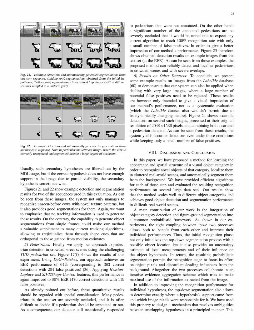
22

Fig. 21. Example detections and automatically generated segmentations fromone cow sequence. (middle row) segmentations obtained from the initial hy-potheses; (bottom row) segmentations from refined hypotheses (with additionalfeatures sampled in a uniform grid).

Fig. 22. Example detections and automatically generated segmentations fromanother cow sequence. Note in particular the leftmost image, where the cow iscorrectly recognized and segmented despite a large degree of occlusion.

Usually, such secondary hypotheses are filtered out by theMDL stage, but if the correct hypothesis does not have enoughsupport in the image due to partial visibility, the secondaryhypothesis sometimes wins.

Figures 21 and 22 show example detection and segmentationresults for two of the sequences used in this evaluation. As canbe seen from these images, the system not only manages torecognize unseen-before cows with novel texture patterns, butit also provides good segmentations for them. Again, we wantto emphasize that no tracking information is used to generatethese results. On the contrary, the capability to generate objectsegmentations from single frames could make our methoda valuable supplement to many current tracking algorithms,allowing to (re)initialize them through shape cues that areorthogonal to those gained from motion estimates.

5) Pedestrians: Finally, we apply our approach to pedes-trian detection in crowded street scenes using the challengingTUD pedestrian set. Figure 17(f) shows the results of thisexperiment. Using DoG+Patches, our approach achieves anEER performance of 64% (corresponding to 363 correctdetections with 204 false positives) [36]. Applying Hessian-Laplace and SIFT/Shape Context features, this performance isagain improved to 80% EER (476 correct detections with 119false positives).

As already pointed out before, these quantitative resultsshould be regarded with special consideration. Many pedes-trians in the test set are severely occluded, and it is oftendifficult to decide if a pedestrian should be annotated or not.As a consequence, our detector still occasionally responded

to pedestrians that were not annotated. On the other hand,a significant number of the annotated pedestrians are soseverely occluded that it would be unrealistic to expect anycurrent algorithm to reach 100% recognition rate with onlya small number of false positives. In order to give a betterimpression of our method’s performance, Figure 23 thereforeshows obtained detection results on example images from thetest set (at the EER). As can be seen from those examples, theproposed method can reliably detect and localize pedestriansin crowded scenes and with severe overlaps.

6) Results on Other Datasets: To conclude, we presentsome example results on images from the LabelMe database[60] to demonstrate that our system can also be applied whendealing with very large images, where a large number ofpotential false positives need to be rejected. Those resultsare however only intended to give a visual impression ofour method’s performance, not as a systematic evaluation(which the LabelMe dataset also wouldn’t permit due toits dynamically changing nature). Figure 24 shows exampledetections on several such images, processed at their originalresolution of 2048×1536 pixels, and combining both a car anda pedestrian detector. As can be seen from those results, thesystem yields accurate detections even under those conditionswhile keeping only a small number of false positives.

VIII. DISCUSSION AND CONCLUSION

In this paper, we have proposed a method for learning theappearance and spatial structure of a visual object category inorder to recognize novel objects of that category, localize themin cluttered real-world scenes, and automatically segment themfrom the background. We have provided efficient algorithmsfor each of those step and evaluated the resulting recognitionperformance on several large data sets. Our results showthat the method scales well to different object categories andachieves good object detection and segmentation performancein difficult real-world scenes.

A main contribution of our work is the integration ofobject category detection and figure-ground segmentation intoa common probabilistic framework. As shown in our ex-periments, the tight coupling between those two processesallows both to benefit from each other and improve theirindividual performances. Thus, the initial recognition phasenot only initializes the top-down segmentation process with apossible object location, but it also provides an uncertaintyestimate of local measurements and of their influence onthe object hypothesis. In return, the resulting probabilisticsegmentation permits the recognition stage to focus its efforton object pixels and discard misleading influences from thebackground. Altogether, the two processes collaborate in aniterative evidence aggregation scheme which tries to makemaximal use of the information extracted from the image.

In addition to improving the recognition performance forindividual hypotheses, the top-down segmentation also allowsto determine exactly where a hypothesis’s support came fromand which image pixels were responsible for it. We have usedthis property to design a mechanism that resolves ambiguitiesbetween overlapping hypotheses in a principled manner. This

23

Fig. 23. Example detections of our approach on difficult crowded scenes from the TUD Pedestrian test set (at the EER). Correct detections are shown in yellow,false positives in red.

mechanism constitutes a fundamental novelty in object detec-tion and results in more accurate acceptance decisions thanconventional criteria based on bounding box overlap.

The core part of our approach is the Implicit Shape Modeldefined in Section IV-C. This implicit representation is flexibleenough that it can combine the information of local objectparts observed on different training examples and interpolatebetween the corresponding objects. As a result, our approachcan learn object models from few examples and achieve com-petitive object detection performance already with training setsthat are between one and two orders of magnitude smaller thanthose used in comparable approaches. Taking a broader view,this implicit model can be seen as a further generalizationof the Hough Transform to work with uncertain data. Inour approach, we have used this capability to represent theuncertainty from intra-class variation, but it would also bepossible to use it with different sources of uncertainty, e.g. forthe identification of known objects under lighting variations.

The run time of the resulting approach mainly dependson three factors: model complexity (the number of codebookentries and occurrences), image size, and the selected searchscale range. Using our current implementation, the single-scale car detector based on Harris points takes between 2-3s for a typical 320 × 240 test image. Typical run-times ofthe pedestrian detector (without our more recent GPU-basedtop-down segmentation) range between 4-7s for the sameimage size, including feature extraction, detection, top-downsegmentation, and MDL verification. We expect that both run-times can still be considerably improved by a more efficientimplementation.

The system can still be extended in several ways. For verylarge scale changes such as the ones encountered in the lastexperiment, it can be advantageous to work on several rescaledversions of the image, simply because of computational ef-ficiency. Other possible extensions include the integrationof multiple cues and the combination of several detectorsfor multi-category discrimination. Finally, many real-worldapplications require that objects be recognized from multipleviewpoints. While this can in principle be achieved by simplystacking several single-view detectors, such an approach wouldnot take advantage of the possibility to share features [69].Extending the ISM approach towards this goal will be a topicof future work.

ACKNOWLEDGMENTS

This work has been funded, in part, by the EU projectsCogVis (IST-2000-29375) and CoSy (IST-2002-004250) andthe Swiss Federal Office for Education and Science (BBW00.0617). We thank Shivani Agarwal for the UIUC car data,Rob Fergus for the CalTech categories, Derek Magee for thecow sequences, Toyota Motor Corporation Europe for thepedestrian data, and Krystian Mikolajczyk for his interest pointdetector and descriptor implementations.

REFERENCES

[1] S. Agarwal, A. Atwan, and D. Roth. Learning to detect objects in imagesvia a sparse, part-based representation. Trans. PAMI, 26(11):1475–1490,2004.

[2] R. Bajcsy, F. Solina, and A. Gupta. Segmentation versus objectrepresentation—are they separable? pages 207–223, 1990.

24

Fig. 24. Example detections on difficult test images from the MIT LabelMe data set [60]. All images were processed at their original resolution of 2048× 1536pixels. The results confirm our approach’s ability to yield accurate detections in such complex scenes with only very few false positives, as the enlargements inthe bottom rows show.

[3] D.H. Ballard. Generalizing the hough transform to detect arbitraryshapes. Pattern Recognition, 13(2):111–122, 1981.

[4] S. Belongie, J. Malik, and J. Puchiza. Shape matching and objectrecognition using shape contexts. Trans. PAMI, 24(4):509–522, April2002.

[5] J.P. Benzecri. Construction d’une classification ascendante hierarchiquepar la recherche en chaıne des voisins reciproques. Cahiers de l’Analysedes Donnees, 7(2):209–218, 1982.

[6] E. Borenstein, E. Sharon, and S. Ullman. Combining top-down andbottom-up segmentations. In Workshop on Perc. Org. in Comp. Vis.,Washington, DC, June 2004.

[7] E. Borenstein and S. Ullman. Class-specific, top-down segmentation. InECCV’02, LNCS 2353, pages 109–122, 2002.

[8] M. Bruynooghe. Methodes nouvelles en classification automatique desdonnees taxinomiques nombreuses. Statistique et Analyse des Donnees,3:24–42, 1977.

25

[9] M.C. Burl, M. Weber, and P. Perona. A probabilistic approach to objectrecognition using local photometry and global geometry. In ECCV’98,1998.

[10] Y. Cheng. Mean shift mode seeking and clustering. Trans. PAMI,17(8):790–799, Aug. 1995.

[11] R. Collins. Mean-shift blob tracking through scale space. In CVPR’03,2003.

[12] D. Comaniciu and P. Meer. Mean shift: A robust approach toward featurespace analysis. Trans. PAMI, 24(5):603–619, 2002.

[13] D. Comaniciu, V. Ramesh, and P. Meer. The variable bandwidth meanshift and data-driven scale selection. In ICCV’01, 2001.

[14] T.F. Cootes, G.J. Edwards, and C.J. Taylor. Active appearance models.In ECCV’98, 1998.

[15] N. Dalal and B. Triggs. Histograms of oriented gradients for humandetection. In CVPR’05, 2005.

[16] W.H.E. Day and H. Edelsbrunner. Efficient algorithms for agglomerativehierarchical clustering methods. J. Classif., 1:7–24, 1984.

[17] C. de Rham. La classification hierarchique ascendante selon la methodedes voisins reciproques. Cahiers de l’Analyse des Donnees, 5(2):135–144, 1980.

[18] T. Deselaers, D. Keysers, and H. Ney. Improving a discriminativeapproach to object recognition using image patches. In DAGM’05, 2005.

[19] G. Dorko and C. Schmid. Selection of scale invariant parts for objectclass recognition. In ICCV’03, 2003.

[20] M. Everingham and others (34 authors). The 2005 pascal visualobject class challenge. In Selected Proceedings of the 1st PASCALChallenges Workshop, LNAI. Springer, 2006 (in press). http://www.pascal-network.org/challenges/VOC/.

[21] P. Felzenszwalb and D. Huttenlocher. Pictorial structures for objectrecognition. IJCV, 61(1), 2005.

[22] R. Fergus, P. Perona, and A. Zisserman. A sparse object category modelfor efficient learning and exhaustive recognition. In CVPR’05, 2005.

[23] R. Fergus, A. Zisserman, and P. Perona. Object class recognition byunsupervised scale-invariant learning. In CVPR’03, 2003.

[24] V. Ferrari, T. Tuytelaars, and L. van Gool. Simultaneous recognitionand segmentation by image exploration. In ECCV’04, 2004.

[25] C. Garcia and M. Delakis. Convolutional face finder: A neural architec-ture for fast and robust face detection. Trans. PAMI, 26(11):1408–1423,2004.

[26] A. Garg, S. Agarwal, and T. Huang. Fusion of global and localinformation for object detection. In ICPR’02, 2002.

[27] C. Harris and M. Stephens. A combined corner and edge detector. InAlvey Vision Conference, pages 147–151, 1988.

[28] B. Heisele, T. Serre, M. Pontil, and T. Poggio. Component-based facedetection. In CVPR’01, pages 657–662, 2001.

[29] P.V.C. Hough. Method and means for recognizing complex patterns.U.S. Patent 3069654, 1962.

[30] M. Jones and T. Poggio. Model-based matching by linear combinationsof prototypes. MIT AI Memo 1583, MIT, 1996.

[31] M.J. Jones and T. Poggio. Multidimensional morphable models:A framework for representing and matching object classes. IJCV,29(2):107–131, 1998.

[32] T. Kadir and M. Brady. Scale, saliency, and image description. IJCV,45(2):83–105, 2001.

[33] B. Leibe, A. Leonardis, and B. Schiele. Combined object categorizationand segmentation with an implicit shape model. In ECCV’04 Workshopon Stat. Learn. in Comp. Vis., 2004.

[34] B. Leibe and B. Schiele. Interleaved object categorization and segmen-tation. In BMVC’03, pages 759–768, Norwich, UK, Sept. 2003.

[35] B. Leibe and B. Schiele. Scale invariant object categorization using ascale-adaptive mean-shift search. In DAGM’04, Springer LNCS, Vol.3175, pages 145–153, 2004.

[36] B. Leibe, E. Seemann, and B. Schiele. Pedestrian detection in crowdedscenes. In CVPR’05, 2005.

[37] A. Leonardis, A. Gupta, and R. Bajcsy. Segmentation of range imagesas the search for geometric parametric models. IJCV, 14:253–277, 1995.

[38] F.-F. Li, R. Fergus, and P. Perona. A bayesian approach to unsupervisedone-shot learning of object categories. In ICCV’03, 2003.

[39] T. Lindeberg. Feature detection with automatic scale selection. IJCV,30(2):79–116, 1998.

[40] D. Lowe. Distinctive image features from scale-invariant keypoints.IJCV, 60(2):91–110, 2004.

[41] D.G. Lowe. Object recognition from local scale invariant features. InICCV’99, 1999.

[42] J. MacQueen. Some methods for classification and analysis of multi-variate observations. In Proceedings of the 5th Berkeley Symposium onMathematical Statistics and Probability, pages 281–297, 1967.

[43] D. Magee and R. Boyle. Detecting lameness using ‘re-samplingcondensation’ and ‘multi-stream cyclic hidden markov models’. Imageand Vision Computing, 20(8):581–594, 2002.

[44] J. Malik, S. Belongie, T. Leung, and J. Shi. Contour and texture analysisfor image segmentation. IJCV, 43(1):7–27, 2001.

[45] D. Marr. Vision. W.H. Freeman, San Francisco, 1982.[46] J. Matas, O. Chum, U. Martin, and T. Pajdla. Robust wide baseline

stereo from maximally stable extremal regions. In BMVC’02, pages384–393, 2002.

[47] C. Mikolajczyk, C. Schmid, and A. Zisserman. Human detection basedon a probabilistic assembly of robust part detectors. In ECCV’04, LNCS3021, pages 69–82. Springer, 2004.

[48] K. Mikolajczyk, B. Leibe, and B. Schiele. Local features for objectclass recognition. In ICCV’05, 2005.

[49] K. Mikolajczyk and C. Schmid. A performance evaluation of localdescriptors. Trans. PAMI, 27(10), 2005.

[50] K. Mikolajczyk, T. Tuytelaars, C. Schmid, A. Zisserman, J. Matas,F. Schaffalitzky, T. Kadir, and L. Van Gool. A comparison of affineregion detectors. IJCV, 65(1/2):43–72, 2005.

[51] A. Mohan, C. Papageorgiou, and T. Poggio. Example-based objectdetection in images by components. Trans. PAMI, 23(4):349–361, 2001.

[52] J. Mutch and D. Lowe. Multiclass object recognition with sparse,localized features. In CVPR’06, 2006.

[53] A. Needham. Object recognition and object segregation in 4.5-month-old infants. J. Exp. Child Psych., 78(3):3–24, 2001.

[54] A. Opelt, M. Fussenegger, A. Pinz, and P. Auer. Weak hypotheses andboosting for generic object detection and recognition. In ECCV’04,2004.

[55] Oxford interest point webpage. http://www.robots.ox.ac.uk/∼vgg/research/affine/detectors.html.

[56] C. Papageorgiou and T. Poggio. A trainable system for object detection.IJCV, 38(1):15–33, 2000.

[57] M.A. Peterson. Object recognition processes can and do operate beforefigure-ground organization. Current Directions in Psychological Science,3:105–111, 1994.

[58] R. Ronfard, C. Schmid, and B. Triggs. Learning to parse pictures ofpeople. In ECCV’02, pages 700–714, 2002.

[59] H. Rowley, S. Baluja, and T. Kanade. Neural network-based facedetection. Trans. PAMI, 20(1):23–38, 1998.

[60] B. Russell, A. Torralba, and W.T. Freeman. The MIT La-belMe Database. http://people.csail.mit.edu/brussell/research/LabelMe, 2005.

[61] C. Schmid and R. Mohr. Combining greyvalue invariants with localconstraints for object recognition. In CVPR’96, 1996.

[62] H. Schneiderman and T. Kanade. Object detection using the statisticsof parts. IJCV, 56(3):151–177, 2004.

[63] S. Sclaroff. Deformable prototypes for encoding shape categories inimage databases. Pattern Recognition, 30(4), 1997.

[64] E. Seemann, B. Leibe, K. Mikolajczyk, and B. Schiele. An evaluationof local shape-based features for pedestrian detection. In BMVC’05,Oxford, UK, 2005.

[65] E. Sharon, A. Brandt, and R. Basri. Fast multiscale image segmentation.In CVPR’00, pages 70–77, 2000.

[66] J. Shi and J. Malik. Normalized cuts and image segmentation. InCVPR’97, pages 731–737, 1997.

[67] C. Stauffer and W.E.L. Grimson. Adaptive background mixture modelsfor realtime tracking. In CVPR’99, 1999.

[68] J. Thureson and S. Carlsson. Appearance based qualitative imagedescription for object class recognition. In ECCV’04, 2004.

[69] A. Torralba, K. Murphy, and W. Freeman. Sharing features: Efficientboosting procedures for multiclass object detection. In CVPR’04, 2004.

[70] Z. Tu, X. Chen, A.L. Yuille, and S-C. Zhu. Image parsing: Unifyingsegmentation, detection, and recognition. In ICCV’03, 2003.

[71] T. Tuytelaars and L. van Gool. Matching widely separated views basedon affinely invariant neighbourhoods. IJCV, 59(1):61–85, 2004.

[72] S. Ullman. Three-dimensional object recognition based on the combi-nation of views. Cognition, 67(1):21–44, 1998.

[73] S. Ullman, M. Vidal-Naquet, and E. Sali. Visual features of interme-diate complexity and their use in classification. Nature Neuroscience,5(7):682–687, 2002.

[74] S.P. Vecera and R.C. O’Reilly. Figure-ground organization and objectrecognition processes: An interactive account. J. Exp. Psych.: HumanPerception and Performance, 24(2):441–462, 1998.

[75] P. Viola and M. Jones. Robust real-time face detection. IJCV, 57(2):137–154, 2004.

[76] M. Weber. Unsupervised Learning of Models for Object Recognition.PhD thesis, California Institute of Technology, Pasadena, CA, 2000.

26

[77] M. Weber, M. Welling, and P. Perona. Towards automatic discovery ofobject categories. In CVPR’00, 2000.

[78] L. Wiskott, J.M. Fellous, N. Krueger, and C. von der Malsburg. Facerecognition by elastic bunch graph matching. Trans. PAMI, 19(7):775–779, 1997.

[79] B. Wu and R. Nevatia. Detection of multiple, partially occluded humansin a single image by bayesian combination of edgelet part detectors. InICCV’05, 2005.

[80] S.X. Yu and J. Shi. Object-specific figure-ground segregation. InCVPR’03, 2003.

[81] A.L. Yuille, D.S. Cohen, and P.W. Hallinan. Feature extraction fromfaces using deformable templates. In CVPR’89, 1989.

[82] J. Zhang, M. Marszalek, S. Lazebnik, and C. Schmid. Local featuresand kernels for classification of texture and object categories: a com-prehensive study. IJCV, 73(2):213–238, 2007.

[83] W. Zhang, B. Yu, G.J. Zelinsky, and D. Samaras. Object classrecognition using multiple layer boosting with heterogenous features.In CVPR’05, 2005.