robust design of lithium extraction from …etd.lib.metu.edu.tr/upload/1027036/index.pdf · robust...
TRANSCRIPT

ROBUST DESIGN OF LITHIUM EXTRACTION FROM BORON CLAYS BY USING STATISTICAL DESIGN AND ANALYSIS
OF EXPERIMENTS
A THESIS SUBMITTED TO THE GRADUATE SCHOOL OF NATURAL AND APPLIED SCIENCES
OF THE MIDDLE EAST TECHNICAL UNIVERSITY
BY ATIL BÜYÜKBURÇ
IN PARTIAL FULFILLMENT OF THE REQUIREMENTS FOR THE DEGREE OF
MASTER OF SCIENCE IN
THE DEPARTMENT OF INDUSTRIAL ENGINEERING
SEPTEMBER 2003

Approval of the Graduate School of Natural and Applied Sciences Prof. Dr. Canan Özgen Director I certify that this thesis satisfies all the requirements as a thesis for the degree of Master of Science.
Prof. Dr. Çağlar Güven Head of Department This is to certify that we have read this thesis and that in our opinion it is fully adequate, in scope and quality, as a thesis for the degree of Master of Science Doç. Dr. Gülser Köksal Supervisor Examining Committee Members
Doç. Dr. Gülser Köksal
Prof. Dr. Ömer Saatçioğlu
Doç. Dr. Sinan Kayalıgil
Doç. Dr. Hakan Gür
Doç. Dr. Refik Güllü

ABSTRACT
ROBUST DESIGN OF LITHIUM EXTRACTION FROM BORON CLAYS BY USING STATISTICAL DESIGN AND ANALYSIS
OF EXPERIMENTS
Büyükburç, Atıl
M.S., Department of Industrial Engineering
Supervisor: Assoc. Prof. Gülser Köksal
September 2003, 144 pages
In this thesis, it is aimed to design lithium extraction from boron clays
using statistical design of experiments and robust design methodologies. There
are several factors affecting extraction of lithium from clays. The most important
of these factors have been limited to a number of six which have been gypsum to
clay ratio, roasting temperature, roasting time, leaching solid to liquid ratio,
leaching time and limestone to clay ratio. For every factor, three levels have
been chosen and an experiment has been designed. After performing three
replications for each of the experimental run, signal to noise ratio
transformation, ANOVA, regression analysis and response surface methodology
have been applied on the results of the experiments. Optimization and
confirmation experiments have been made sequentially to find factor settings
that maximize lithium extraction with minimal variation. The mean of the
maximum extraction has been observed as 83.81% with a standard deviation
of 4.89 and the 95% prediction interval for the mean extraction is (73.729,
94.730). This result is in agreement with the studies that have been made in
iii

the literature. However; this study is unique in the sense that lithium is extracted
from boron clays by using limestone directly from the nature, and gypsum as a
waste product of boric acid production. Since these two materials add about 20%
cost to the extraction process, the results of this study become important.
Moreover, in this study it has been shown that statistical design of experiments
help mining industry to reduce the need for standardization.
Keywords: Statistical Design of Experiments, Taguchi Method, Robust Design,
Response Surface Methodology, Lithium Extraction, Boron Clays
iv

ÖZ
BOR KİLLERİNDEN LİTYUM KAZANIMININ İSTATİSTİKSEL DENEY TASARIMI VE ANALİZİ YOLUYLA
ROBUST TASARIMI
Büyükburç, Atıl
Yüksek Lisans, Endüstri Mühendisliği Tez Yöneticisi: Doç. Dr. Gülser Köksal
Eylül 2003, 144 Sayfa
Bu tez çalışmasında, bor killerinden lityumun kazanılmasının,
istatistiksel deney tasarımı ve robust tasarım metotları uygulanarak tasarlanması
amaçlanmıştır. Lityumun killerden kazanımı etkileyen çeşitli faktörler vardır.
Bunlar içinde en önemlileri altı faktörde sınırlanmıştır. Bunlar jipsin kile oranı,
kavurma sıcaklığı, kavurma süresi, liçin katı sıvı oranı, liç süresi, kireçtaşının
kile oranıdır. Her parametre için üç seviye seçilecek şekilde, deney
tasarlanmıştır. Her deney için üç tekrar yapıldıktan sonra, sinyal/gürültü oranı
dönüşümü, ANOVA, regresyon analizi ve cevap yüzeyi metotları, deney
sonuçları üzerinde uygulanmıştır. En yüksek lityumun çözünmesini ve en düşük
sapmayı sağlayacak faktör seviyelerinin bulunması için optimizasyon ve
doğrulama deneyleri bir önceki sonuçlar kullanılarak yapılmıştır. Deneyler
sonucunda ortalama lityum kazanımı %83.81 olurken, standard sapma 4.89
olarak hesaplanmış, %95 tahmin aralığı ise (73.729, 94.730) olarak
bulunmuştur. Elde edilen bu sonuçlar, literatürde yapılmış olan killerden lityum
kazanımı çalışmaları ile uyumluluk göstermektedir. Ancak bu çalışmada
killerden lityum kazanımına yeni bir bakış açısı getirilmiş ve proses esnasında
kullanılan kireçtaşının doğrudan doğadan sağlanması, jips olarak ise borik asit
v

üretiminde açığa çıkan katı atığın kullanılması düşünülmüştür. Bu iki
hammaddenin toplam proses ekonomisine yaklaşık %20’lik bir maliyet
getirdiği göz önüne alındığında çok önemli olduğu düşünülmektedir. Ayrıca bu
çalışmada madencilik sektöründe standardizasyona duyulan ihtiyacın
istatistiksel deney tasarımının yardımıyla azaltılabileceği gösterilmiştir.
Anahtar Kelimeler: İstatistiksel Deney Tasarımı, Taguchi Metodu, Robust
Tasarım, Cevap Yüzeyi Metodolojisi, Lityum Kazanımı, Bor Killeri
vi

To Uğur and Berin Büyükburç
vii

ACKNOWLEDGEMENTS
I would like to express sincere apprecation to Assoc. Prof. Gülser
Köksal, Head of R&D Department of Eti Holding, Dr.Muhittin Gündüz,
Director of Proses and Pilot Facility of R&D Department, Uğur Bilici, Director
of Laboratory, Tahsin Tufan, on the behalf of all laboratory personel, Derya
Maraşlıoğlu and my parents. Assoc. Prof. Gülser Köksal introduced me the
subject and supervised throughout the thesis. Dr. Muhittin Gündüz and Uğur
Bilici let me make such a research in the R&D Department and helped me
throughout the study. Tahsin Tufan and Derya Maraşlıoğlu with all other
laboratory personel did their best to do the analyses on time and as soon as
possible. Finally my parents encouraged me to continue and have my M.S.
Degree.
viii

TABLE OF CONTENTS
ABSTRACT ……………………………………………………………… iii
ÖZ ………………………………………………………………………... v
ACKNOWLEDGEMENTS ………………………………………………. viii
TABLE OF CONTENTS ………………………………………………… ix
LIST OF TABLES ………………………………………………………… xi
LIST OF FIGURES ………………………………………………………. xiii
CHAPTER
1. INTRODUCTION ………………………………………………… 1
2. LITERATURE SURVEY ………………………………………… 4
2.1 Background on Lithium Extraction …………………………. 4
2.2 Background on Design and Analysis of Experiments
for Optimization ..……………………………………….…... 9
3. PROBLEM DEFINITION AND EXPERIMENTAL
PROCEDURE ……………………………………………………... 20
3.1 Raw Material Preparation …………………………………... 23
3.2 Roasting ……………………………………………………... 24
3.3 Leaching ……………………………………………………... 26
4. DESIGN, CONDUCT AND ANALYSIS OF THE
EXPERIMENTS …………………………………………………... 29
4.1 Design and Conduct of Experiments ……………………….. 29
4.1.1 Deciding on the Levels of Control Factors …………….. 29
4.1.2 Designing the Experimental Layout …………………... 31
ix

4.2 Regression Analysis ………………………………………….. 46
4.2.1 Modelling the Mean Response …………………………... 46
4.2.2 Modelling the Standard Deviation ……………………… 56
5. OPTIMIZATION ……………………………………………………. 68
5.1 Minitab Response Optimizer ………………………………… 69
5.2 GAMS Non-Linear Programming ……………………………. 72
5.3 Ridge Analysis ………………………………………………. 75
5.4 Optimization Outside the Response Surface …………………. 77
6. AN ATTEMPT TO IMPROVE THE OPTIMUM POINT …………. 80
6.1 An Improved Experimental Design and Analysis ……………. 80
6.2. Comparison of Results to Relevant Literature Work ……….. 92
7. ECONOMIC IMPACT AND ANALYSIS OF THE STUDY ……… 94
8. CONCLUSION AND SUGGESTIONS FOR FUTURE WORK …. 98
LIST OF REFERENCES ……………………………………………………. 103
APPENDICES ……………………………………………………………... 107
x

LIST OF TABLES
TABLE
3.1. Factors Affecting the Extraction of Lithium ……………………… 21
3.2. The Chemical Analyses of Raw Materials ……………………….. 23
4.1. The Levels of the Factors ………………………………………… 31
4.2. The Assignment of Factors to the Columns of L27 (313) Array …… 32
4.3. The Results of the Experiments …………………………………... 34
4.4. The Average, Standard Deviation and S/N Ratio of Experiments ... 35
4.5. ANOVA of S/N Ratio Values ……………………………………... 36
4.6. ANOVA of S/N Ratio without Interaction Terms …………………. 38
4.7. ANOVA of S/N Ratio without Interaction Terms and Gypsum …… 39
4.8. Level Averages of Factors ………………………………………… 40
4.9. ANOVA Table for the Mean ……………………………………... 42
4.10. ANOVA Table for the Standard Deviation ……………………… 43
4.11. ANOVA for Regression Analysis for the Mean Including Only
Main Factors ……………………………………………………… 46
4.12. Significance of β Terms of the General Linear Model [4.5] ……... 48
4.13. ANOVA for Regression Analysis for the Mean Including Main,
Interaction and Square Factors …………………………………… 49
4.14. Significance of β Terms of Quadratic Model …………………….. 51
4.15. ANOVA for the Improved Quadratic Regression Model [4.7] …... 52
4.16. Significance of β Terms of the Improved Quadratic Model [4.7] ... 54
4.17. ANOVA for Quadratic Regression Analysis for the Standard
Deviation …………………………………………………………. 56
4.18. Significance of β Terms of Quadratic Model [4.8] ………………. 58
xi

4.19. ANOVA for Quadratic Regression Analysis for Modelling
log s2 ……………………………………………………………... 59
4.20. Significance of β Terms of Quadratic Model [4.9] for log s2 ……... 61
4.21. ANOVA for Improved Quadratic Regression Analysis for log s2 … 62
4.22. Significance of β Terms of Improved Quadratic Model [4.10]
for log s2 …….……………………………………………………... 64
4.23. ANOVA for Cubic Regression Analysis for log s2 ……………….. 65
4.24. Significance of β Terms of Cubic Regression Model for log s2 …... 67
5.1. The Prediction Intervals for Mean and Standard Deviation
Computed by MINITAB Response Optimizer …………………… 70
5.2. Mean Values Computed from GAMS and Standard Deviation with
Prediction Intervals for both Mean and log s2 Computed by
MINITAB Response Optimizer …………………………………… 74
5.3. The Optimum Points Found by GAMS Outside the Experimental
Region ……………………………………………………………... 78
6.1. The Points That Have Been Added to the Model …………………. 81
6.2. ANOVA for Regression Analysis for Model Comprising Optimum
Points ………………………………………………………………. 81
6.3. Significance of β Terms of the Model [6.1] Including Optimum
Points ………………………………………………………………. 84
6.4. ANOVA for Regression Analysis for Model of log s2 Comprising
Optimum Points …………………………………………………… 85
6.5. Significance of β Terms of the Regression Model [6.2] Including
Optimum Points for log s2 …………………………………………. 87
6.6. The Prediction Intervals for Mean and Standard Deviation Computed
by MINITAB Response Optimizer ………………………………... 88
6.7. Comparison of Results to Other Studies …………………………… 92
7.1. Comparison of operating cost of the proposed lithium extraction
process to that of Crocker et. al. (1988) ………………………………….. 95
xii

LIST OF FIGURES
FIGURE
2.1. The Extraction of Li2CO3 and Other Salts From Brines, Salar de
Atacama, Chile ……………………………………….……………... 6
2.2. The Process Flowchart of Li2CO3 From Hectorite Clay ……………. 8
2.3. General Model of a Process ………………………………………… 11
2.4. The Flow Diagram of Response Surface Methodology …………….. 18
2.5. Contour Plot and a Response Surface ………………………………. 19
3.1. Pictures of Raw Materials and Grinding Machine …………………. 24
3.2. The Muffle Furnace and Roasts in the Crucible …………………….. 25
3.3. The Picture of Reactor and Cryostat ………………………………... 27
3.4. The Process Flowchart Used in This Study ………………………… 28
4.1. The Interaction Plot for Roasting Temperature x Gypsum …………. 36
4.2. The Interaction Plot for Roasting Temperature x Roasting Time ….. 37
4.3. The Interaction Plot for Roasting Temperature x Leach S/L Ratio … 37
4.4. The Residuals versus Fitted Values of the Model Found by
ANOVA for S/N Ratio ……………………………………………... 39
4.5. Normal Probability Plot for the Model Found by
ANOVA for S/N Ratio ……………………………………………... 40
4.6. Main Effects Plots of Signal-to-Noise Ratio ……………………….. 41
4.7. Residual versus Fitted Values of the Residuals of General
Linear Model [4.5] with only Main Factors ………………………… 47
xiii

4.8. Normal Probability Plot of the Residuals of General Linear
Model [4.5] with only main Factors ……………………………….. 47
4.9. Residual vs Fitted Values of the Residuals of Quadratic
Model [4.6] with Interaction Factors ………………………………. 50
4.10. Normal Probability Plot of the Residuals of Quadratic
Model [4.6] with Interaction Factors ……………………………... 50
4.11. Residual vs Fitted Values of the Residuals of Improved Quadratic
Model [4.7] ……………………………………………………….. 53
4.12. Normal Probability Plot of the Residuals of Improved Quadratic
Model [4.7] ……………………………………………………….. 53
4.13. Residuals versus Fitted Values Plot of the Quadratic Regression
Model [4.8] for the Standard Deviation ………………………….. 57
4.14. Normal Probability Plot of the Quadratic Regression
Model [4.8] for the Standard Deviation …………………………... 57
4.15. Residuals versus Fitted Values Plot of the Quadratic
Regression Model [4.9] for log s2 ………………………………… 60
4.16. Normal Probability Plot of the Quadratic Regression
Model [4.9] for log s2 …………………………………………….. 60
4.17. Residuals versus Fitted Values Plot of the Improved Quadratic
Regression model [4.10] for log s2 ………………………………... 63
4.18. Normal Probability Plot of the Improved Quadratic Regression
Model [4.10] for log s2 …………………………………………… 63
4.19. Residuals versus Fitted Values Plot of the Cubic Regression
Model [4.11] for log s2 …………………………………………… 66
4.20. Normal Probability Plot of Cubic Model [4.11] for log s2 ……….. 66
6.1. The Residuals versus Fitted Values Plot for the Regression
Model [6.1] Including Optimum Points …………………………… 82
xiv

6.2. The Normal Probability Plot of Residuals for the Regression
Model [6.1] Including Optimum Points …………………………….. 82
6.3. The Residual versus Fitted Values Plot for the Regression Model
of log s2 [6.2] Including Optimum Points ………………………….. 86
6.4. The Normal Probability Plot of Residuals for the Regression Model
of log s2 [6.2] Including Optimum Points ………………………….. 86
6.5. Contour Plot of Roasting Temperature versus Leaching Solid to
Liquid Ratio for Mean ………………………………………………. 91
6.6. Contour Plot of Roasting Temperature versus Leaching Solid to
Liquid Ratio for log s2 ………………………………………………. 91
xv

CHAPTER I
INTRODUCTION
The aim of this study is to use statistical experimental design and
analysis of these experiments in order to maximize the extraction of lithium
from the clays of the boron fields. While achieving this aim, it is tried to make
the lithium extraction robust to the variations in the process. Taguchi’s L27 (313)
orthogonal array has been chosen as the statistical experimental design. In order
to analyse the robustness of the process, three replications have been performed.
Signal-to-Noise (S/N) ratio, Analysis of Variance (ANOVA) and Regression
Analysis (for both mean and standard deviation) and Response Surface
Methodology have been used in order to maximize the mean of lithium
extraction and minimize the variation.
The widest application areas of lithium and its compounds are in several
industries such as glass, ceramics, lubricants, pharmaceutics, metallurgy and
batteries (Fishwick, 1974). In the ceramic industry, lithium is used as an additive
to frits and glazes to reduce the viscosity. In the pharmaceutics industry, it is
used in the synthesis of vitamin A and in the treatment of manic-depressive
disorders. As lithium has high energy density, it is a desirable electrode material
in batteries. Lithium compounds like lithium carbonate (Li2CO3) is added to the
aluminium electrolysis cells in order to increase current efficiency and thereby
decreasing the power consumption (Fishwick, 1974).
1

It is known that lithium occurs in boron fields (Mordoğan et. al., 1995,
Beşkardeş et. al., 1992 and Büyükburç et. al., 2002) all of which owned by a
state-hold company, Eti Holding, Inc. Therefore, from the clays of boron
minerals, lithium has been tried to be extracted and production of Li2CO3 has
been aimed. In this study a different approach has been suggested for the
extraction process design. This approach has been based on using raw materials
that can be obtained from the facilities and fields of Eti Holding, Inc. Therefore,
the raw material cost will be minimized so that no payment will be made for
purchasing these raw materials. The studies in literature have not used or have
not had any chance to use such an approach.
There are several factors affecting the Li2CO3 production from clays.
The production steps can be simplified as pelletizing, roasting, leaching,
evaporation, precipitation and filtering.
The first and main part of the process is to take lithium into the solution.
The most important parameters of taking lithium into solution can be classified
as; raw material to clay ratio, roasting temperature, roasting time, leaching time
and leaching solid to liquid ratio. In order to perform the experiments, three
levels for each factor have been determined and Taguchi’s L27(313) orthogonal
array is chosen in order to estimate the main effects and some of interactions. To
perform robust analysis and study the variations, three replications for each run
have been obtained. S/N ratio has been estimated and analysis of variance
(ANOVA) has been performed. The regression analyses for both the mean and
the standard deviation have been conducted. In order to achieve the maximum
solubility, response surface methodology has been used and it has been tried to
find the global optimum of extraction by employing the GAMS non-linear
programming and the methodology of response surfaces for 2nd order surfaces,
Ridge Analysis. Although after completing the designed experiments maximum
extraction has been identified as 73%, applying optimization methods has
increased the extraction to about 83% on the average. These methodologies have
not been applied commonly in mining industry, without making any
standardization to the best of our knowledge.
2

In Chapter II, the background on the methods used in this study has been
provided. In Chapter III, problem definition and the experimental procedure
have been explained. In Chapter IV, the design, analysis and conduct of
experiments have been explained. In Chapter V, the optimization study has been
reported. In Chapter VI, an attempt to improve the optimum points has been
presented. In Chapter VII, a cost analysis for this study has been made. Finally
in Chapter VIII, the results obtained from this study have been discussed and
suggestions for future work have been made.
3

CHAPTER II
LITERATURE SURVEY
2.1. Background On Lithium Extraction
In this study, lithium has been extracted from boron fields by applying
roasting and leaching processes simultaneously, and the experiments have been
performed by using orthogonal arrays, and analysis of experiments (ANOVA,
Regression) has been performed. On the results gained from regression,
response surface and robust design methodologies have been applied.
Lithium is the third element of the periodic table coming after hydrogen
and helium. It is the lightest metal and its atomic weight is 6.938. The name
lithium originates from the Greek word “lithos” that means stone. The first
identification of lithium was in the 19th century by Johan August Arfvedson.
Arfvedson had analysed the content of a mineral later called spodumene
[LiAl(Si2O6)] and saw that an accounted portion of the ore was not identified
(Kroschwitz, 1994). Further work resulted in extraction of a compound that had
unknown chemical properties. However; it was not until 1855 that lithium was
extracted as a free metal by the studies of Robert Bunsen and Augustus
Matthienson. They achieved these by electrolysis of lithium chloride. In 1923,
Metallgesellschaft AG in Germany did the first commercial production of
lithium. The first production of lithium on an appreciable scale was during
1900’s as spodumene mineral of Etta Mine in the Black Hills of South Dakota.
The large increase of lithium and its derivatives production were in the middle
of 1950’s due to the thermonuclear program of Atomic Energy Commission
(AEC). The program had been completed in 1960 and the lithium producers
have been left with an excess capacity. However; after 1960 new application
4

areas of lithium were found.
The average concentration of lithium in earth’s crust is about 0,006%
and it is supposed that there exists 0,1 ppm lithium in seawater. The main
sources of lithium are clays, minerals and brines. However; current commercial
production is made from minerals and brines. The commercially important
lithium minerals are spodumene, lepidolite, petalite and amblygonite (Saller and
O’Driscoll, 2000). These minerals are either used directly in certain applications
or they are converted in the lithium compounds such as Li2CO3, LiCl, LiOH.
Li2CO3 production is made both from minerals and brines. The production is
made mainly from brines as this is easier and cheaper than mineral processing.
A smectit-type clay which contained minimum lithium content of about
4500 ppm is called hectorite. This type of clay is not currently used for
producing lithium but instead is used directly in different applications. Some
studies were performed (Lien, 1985, May et. al., 1980 and Edlund, 1983) in
order to extract lithium from these clays and then producing Li2CO3.
Lithium carbonate (Li2CO3) is the most important compound of lithium,
which is a raw material for various industries as explained in Chapter 1. Li2CO3
is produced commercially from minerals and brines. The production route from
minerals includes crushing of spodumene mineral and applying of flotation in
order to produce concentrate. Then the concentrate goes through a heating
process at about 1100°C and the crystal structure of spodumene is altered so it
becomes more reactive to sulfuric acid. The mixture of finely ground converted
spodumene and sulfuric acid is heated to 250°C and forms lithium sulphate
which is a water soluble compound. After leaching with water, insoluble
compounds are separated by filtration. Lithium carbonate is achieved by reacting
lithium sulphate and sodium carbonate (Na2CO3) (Ober, 2001). As this process
is energy intensive, producing lithium carbonate is expensive when compared
with the production from brines and the production is shifting to that side. The
production from brines mainly includes evaporation, filtration, and precipitation
steps. The schematic diagram of Li2CO3 production from the world’s largest
lithium containing brine (Salar de Atacama, Chile), is shown in Figure 2.1.
5

Li2CO3 Precipitation
NaCl
Cake (NaCl, KCl) (KCl)
Cake (K/ Mg/ Li Sulphate) K2SO4
Mg and impurities
Na2CO3
H3BO3
Li2CO3
Figure 2.1. The extraction of Li2CO3 and other salts from brines, Salar de
Atacama, Chile (Mordoğan et. al., 1995 and Coad, 1984)
6
Brine
Evaporation Pond
Filtration
Evaporation Pond
Filtration KCl plant
Evaporation Pond
Filtration
Li plant (Chem. Proc.)
Boric Acid plant
K2SO4 plant
Washing, drying, packing
Ooi et. al. (1986) have claimed that if the application of lithium in
thermonuclear fusion will come to the stage, the known lithium reserves will not
be enough to supply this demand, and extraction of lithium from the sea water
will be needed regardless of the low concentration which is 0.17 ppm. However;
before coming to the extraction from sea water, the recovery from lithium
bearing clays are to be thought. By this point of view, various studies have been
performed in order to extract lithium from clays. The methods to extract lithium
can be classified as water disaggregation, sulfuric acid leaching, acid baking-
water leaching, alkaline roast-water leach, sulfate roast-water leach, chloride
roast-water leach, multiple reagent roast-water leach (May et. al., 1980),
selective chlorination (Davidson, 1981) and lime-gypsum roasting-water leach
(Edlund, 1983 and Lien, 1985). Among all these, lime-gypsum roasting-water
leach is the most promising method. Edlund (1983) tries to optimize the lime-
gypsum ratios and roasting parameters. He conducts the experiment in different
atmospheres such as N2+CO atmosphere, CO+H2O+N2 atmosphere.
Clay:Lime:Gypsum ratio 5:3:3 is found as the optimum. The calcination time is
prolonged to 4 hours and experiments are conducted for hours between 1-4. The
results indicate that calcination temperature of 900°C yields the best results for
batch production with a rotary furnace. According to the same study, in an
electrically heated furnace the extraction yield has increased for all
temperatures. Lien (1985) makes an extensive study for producing Li2CO3 from
a montmorillonite-type clay containing %0,6 lithium. He also sets the
clay:lime:gypsum ratio to 5:3:3 as optimum and conducts the experiments in the
calcination temperature range of 750-1100°C for 1 hour. Lien (1985) concludes
that 78-82% of lithium in the clay can be recovered. He also estimates the
production cost of Li2CO3 and finds the cost as 1.4 fold larger than market price
of Li2CO3. The process flow chart is given in Figure 2.2.
7

Lithium containing clay
Limestone (CaCO3) Gypsum (CaSO4.2H2O)
Pelletized Raw Material
Wash Water
Water Slurry
Residue
Leach Solution
CaCO3
Concentrated Solution
Na2CO3
Slurry
Li2CO3
Figure 2.2. The process flowchart of Li2CO3 from hectorite clay (Lien, 1985)
8
Raw Material Preparation
Roasting
Water Leaching
Filtration
Evaporator
Filtration
Li2CO3 Precipitation
Filtration

Extraction of lithium from boron fields has been the subject of Turkish
researchers (Mordoğan et.al, 1995 and Beşkardeş et.al, 1992). Mordoğan et. al.
(1995) conclude that 77% of lithium from Kırka clays can be recovered by
adding 16,67% gypsum to the clay but no lime. Calcination temperature and
time set as 900°C and 2 hours as optimum. Leaching time and solid:liquid ratio
used are 1 hour and 0.1 respectively. Beşkardeş et. al. (1992) mainly concern
with the application of Bigadiç clays for industrial use and try to investigate the
economy of recovering lithium. They conclude that the cost of recovering
lithium is 10,95$/kg which is about 3 times the selling price of Li2CO3.
2.2. Background on Design and Analysis of Experiments for
Optimization
In this study, natural lime-waste gypsum roasting-water leach method
has been used in order to extract lithium from boron fields. The experiments
have been performed by using Taguchi’s L27 (313) orthogonal array and analysed
by using robust design methodologies. S/N Ratio, ANOVA, regression and
response surface are the methods that have been used to analyse the experiments
and optimize the extraction of lithium.
After World War II, Japan faced the problem of reconstruction the
country. The main problem was from good-quality raw material, high-quality
manufacturing equipment and skilled engineers (Phadke, 1989). To meet this
challenge, Genichi Taguchi was assigned and he developed the foundations of
Robust Design. The Robust Design method provides a systematic and efficient
approach in order to get close to the optimum by having the product functional,
exhibiting high performance and robust to variations (Erdoğan, 2000).
The robust design methodology strives for:
1. Making product performance insensitive to raw material which in turn
leads to independence from the grade or quality of the raw material or
components in the process.
9

2. Making the design robust to the manufacturing variation in order to
reduce labor and material cost for rework.
3. Having the design less sensitive to operating environment so that the
reliability improves and operating cost decreases.
4. Using a novel development process, which will help, in using the
engineering time more productively.
In order to achieve these aims, robust design simply tries to minimize the
sensitivity of the process or product to the variation caused by uncontrollable
factors without sacrificing the main aim, optimizing the mean (minimize,
maximize or on target). The optimum settings of the controllable factors are
found and set to minimize the variation. Robust Design involves eight steps
which can be grouped into three categories as planning experiments, conducting
them and analyzing and conforming the results (Phadke, 1989).
Planning the experiment contains;
a- Identifying of the main function
b- Identify noise factors and testing conditions for quality loss
c- Decide on the quality characteristic to observe and the objective
function to be optimized
d- Identifying and levelling of the control factors
e- Choosing the most suitable experiment design and data analysis
procedure
Performing the experiments contains;
f- Conducting the experiments
Analyzing and conforming the results consists of;
g- Analyzing the data and determining of optimum levels for control
factors
h- Conduct the confirmation experiments and planning future actions
The Robust Design method developed by Taguchi has two major tools;
signal-to-noise ratio and orthogonal arrays.
10
When we intentionally deal with the problem of minimizing the variation
and the optimization of the response simultaneously, we can transform our data
such that we can observe the variation and the mean. Taguchi recommended the
transformation of the raw data to signal-to-noise ratio (S/N). S/N ratio
consolidates several repetitions (at least two data points are required) into one
value which reflects the amount of variation (Ross, 1988). In Robust Design,
S/N ratio is used as the objective function to be maximized.
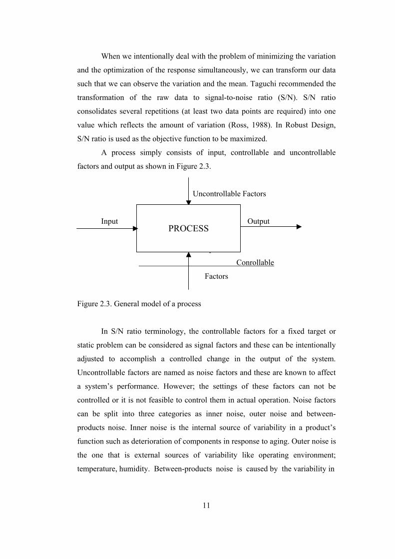
A process simply consists of input, controllable and uncontrollable
factors and output as shown in Figure 2.3.
Uncontrollable Factors
Input Output
Input
Conrollable
Factors
Figure 2.3. General model of a process
In S/N ratio terminology, the controllable factors for a fixed target or
static problem can be considered as signal factors and these can be intentionally
adjusted to accomplish a controlled change in the output of the system.
Uncontrollable factors are named as noise factors and these are known to affect
a system’s performance. However; the settings of these factors can not be
controlled or it is not feasible to control them in actual operation. Noise factors
can be split into three categories as inner noise, outer noise and between-
products noise. Inner noise is the internal source of variability in a product’s
function such as deterioration of components in response to aging. Outer noise is
the one that is external sources of variability like operating environment;
temperature, humidity. Between-products noise is caused by the variability in
11
PROCESS

the manufacturing procedures or equipment. Welding amperage can be an
example for such a noise.
Using S/N ratio we can simply analyze the results of the experiments
involving multiple runs, instead of extended and time-consuming analysis. S/N
ratio lets the selection of the optimum objective with minimum variation around
the target.
A classical example can be given to show the idea of S/N ratio. Let us
consider a radio that the signal factor is the power of the radio signal and
noise factor is interference of storm. The clearness of radio signal is the target
and the storm interference is variation. The most desirable situation is strong
signal and little interference whereas the least desirable situation is weak signal
and strong interference. So maximizing radio signal/storm interference will be
the most suited case for our problem.
There are three types of S/N ratios for static cases;
- Nominal-the-Best
- Smaller-the-Better
- Larger-the-Better
Nominal-the-Best: Nominal-the-best is the correct type when we have the
following conditions;
L: Quality Loss = 0 when µ:Target=m, and σe:Deviation=0
To simplify, nominal-the best is a measurable characteristic with a specific user-
defined target. The transformation to S/N ratio can be made by the following
formula:
where;
η = symbol for S/N; (dB)
12
[2.1]2
210syLOG=η
n
ymeany
n
ii∑
=== 1 n= number of data points, yi = the result of the ith data
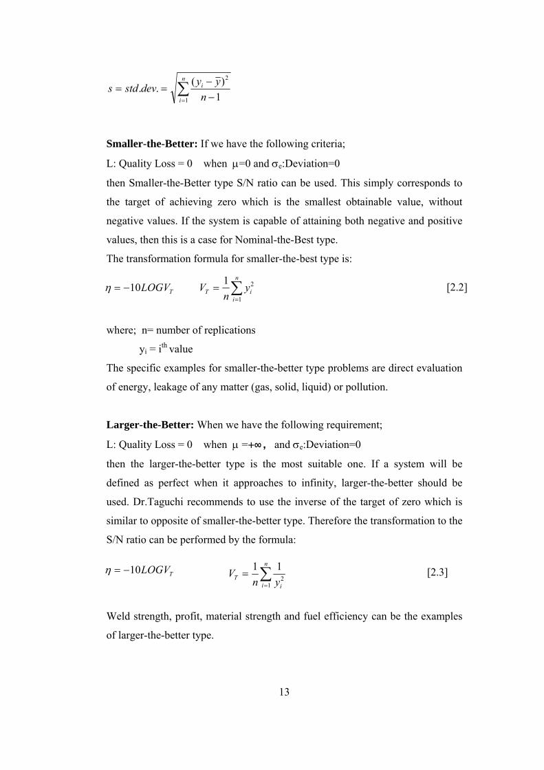
Smaller-the-Better: If we have the following criteria;
L: Quality Loss = 0 when µ=0 and σe:Deviation=0
then Smaller-the-Better type S/N ratio can be used. This simply corresponds to
the target of achieving zero which is the smallest obtainable value, without
negative values. If the system is capable of attaining both negative and positive
values, then this is a case for Nominal-the-Best type.
The transformation formula for smaller-the-best type is:
where; n= number of replications
yi = ith value
The specific examples for smaller-the-better type problems are direct evaluation
of energy, leakage of any matter (gas, solid, liquid) or pollution.
Larger-the-Better: When we have the following requirement;
L: Quality Loss = 0 when µ =+∞, and σe:Deviation=0
then the larger-the-better type is the most suitable one. If a system will be
defined as perfect when it approaches to infinity, larger-the-better should be
used. Dr.Taguchi recommends to use the inverse of the target of zero which is
similar to opposite of smaller-the-better type. Therefore the transformation to the
S/N ratio can be performed by the formula:
Weld strength, profit, material strength and fuel efficiency can be the examples
of larger-the-better type.
13
TLOGV10−=η ∑=
=n
iiT y
nV
1
21
TLOGV10−=η ∑=
=n
i iT yn
V1
2
11
[2.2]
[2.3]
∑= −
−==
n
i
i
nyydevstds
1
2
1)(..
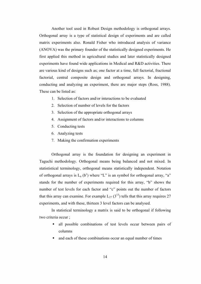
Another tool used in Robust Design methodology is orthogonal arrays.
Orthogonal array is a type of statistical design of experiments and are called
matrix experiments also. Ronald Fisher who introduced analysis of variance
(ANOVA) was the primary founder of the statistically designed experiments. He
first applied this method in agricultural studies and later statistically designed
experiments have found wide applications in Medical and R&D activities. There
are various kind of designs such as; one factor at a time, full factorial, fractional
factorial, central composite design and orthogonal arrays. In designing,
conducting and analyzing an experiment, there are major steps (Ross, 1988).
These can be listed as:
1. Selection of factors and/or interactions to be evaluated
2. Selection of number of levels for the factors
3. Selection of the appropriate orthogonal arrays
4. Assignment of factors and/or interactions to columns
5. Conducting tests
6. Analyzing tests
7. Making the confirmation experiments
Orthogonal array is the foundation for designing an experiment in
Taguchi methodology. Orthogonal means being balanced and not mixed. In
statististical terminology, orthogonal means statistically independent. Notation
of orthogonal arrays is La (bc) where “L” is an symbol for orthogonal array, “a”
stands for the number of experiments required for this array, “b” shows the
number of test levels for each factor and “c” points out the number of factors
that this array can examine. For example L27 (313) tells that this array requires 27
experiments, and with these, thirteen 3 level factors can be analysed.
In statistical terminology a matrix is said to be orthogonal if following
two criteria occur ;
all possible combinations of test levels occur between pairs of
columns
and each of these combinations occur an equal number of times
14
There are several orthogonal arrays that are used. The most widely
ones are L4(23), L8(27), L9(34), L12(211), L16(45), L18 (21x37), L25(56), L27(313) and
L32(231). There are other orthogonal arrays that are less common such as
L20(219), L98(715x21), L121(1112), L169(1314). It is possible to create new
orthogonal arrays by merging colums of the most widely used ones. Some
examples for such arrays are; L18(61x36), L27(91x39), L81(910) and L128(441x24).
Ünal (2001) lists all these orthogonal arrays and in Phadke (1989), interaction
tables and linear graphs of the most commonly used arrays can be found.
After performing the experiments, the analysis and model fitting of the
experimental data come into nature. Model fitting is made by using regression.
Regression analysis is called simple regression when the model contains only
one factor. If there are more than one factor in the model, then multiple
regression is performed to fit a model. When the model contains only linear
terms then this model fitting is called multiple linear regression, and denoted by:
y = β0 + β1X1 + β2X2 + ...+ βkXk + ε [2.4]
When the model contains square and interaction terms then the model is called
quadratic regression and the model is formulated as:
In order to find the optimum point in the model, response surface
methodology can be used. An experimenter wishes to have the optimum point in
his/her experimental region. An appropriate way to see whether the global
optimum lies in the experimental region is to apply response surface methods.
For a regression problem including only the linear terms in xj’s, it is easy for
response methodology to reach to optimum by using the method called steepest
ascent. This method basically tries to reach the optimum by moving b1 units in,
say X1 direction for every b2 units in, say X2 direction starting at the centre
15
[2.5]
2
11 110 j
k
jjjmj
k
j
k
mjmj
k
jj xxxx ∑∑∑∑
== ==
+++= ββββη
for j<m

(0,0) of the experimental design if X1 and X2 are the only variables. Thus, the
steps along the path are proportional to the regression coefficients (βi’s)
(Montgomery, 1997). If second order model is necessary to explain the
relationship, ridge analysis can be used.
The technique of ridge analysis was first suggested by A.E.Hoerl (1959)
and later urged by R.W.Hoerl (1985). It is developed form of the steepest ascent
that will apply to second-order surfaces and finds its origin in Box and Wilson
(1951) (Box and Draper, 1987).
The method simply comprises the following:
Consider the 2nd order response surface in k variables x1, x2,...,xk that
µ = b0 + b1x1 + b2x2 + ... + bkxk + b11x12 + b22x2
2 + ... + bkkxk2 +
b12x1x2 + b13x1x3 + ... +bk-1,kxk-1xk [2.6]
Suppose a sphere centring at the origin [usually (0,0,...,0)] and having
radius R is drawn. Then it is certain that somewhere in the sphere there will be a
maximum and elsewhere a minimum. Also depending on the type of quadratic
surface [2.6] values of µ which are local maxima or minima, that is maxima and
minima for all nearby points on the sphere, but not absolute maxima or minima
when all points of the sphere are taken into consideration (Box and Draper,
1987).
For ridge analysis, application of the method of Lagrange multipliers
leads to the following equations, which must be solved for x = (x1, x2,…,xk)/:
(B- λI) x = -1/2 b [2.7]
b11 1/2b21 ... 1/2b1k
1/2b12 b22 ... 1/2b2k
... ... ... ...
1/2b1k 1/2b2k ... bkk
16
B=
b=
b1 b2 ... bk

Let the eigenvalues of the matrix B be denoted by µi (i=1,...,k). Then, det (B-
µI) = 0 will provide the eigenvalues. Suppose that the largest eigenvalue for B is
µL and the smallest eigenvalue is µs. Some assignment values to λ is given and
equation [2.7] is solved and values for x1, x2,...,xk are computed. Whether the
assigned λ value is outside the interval [µs µL] or inside the interval gives the
decision of the point, x = (x1, x2,...,xk) as local or global maxima or minima
(Box and Draper, 1987).
Contour plots and response surface graphs are two basic constitutes of
response surface methodologies that help the researcher visualise the surfaces
more easily. An example adapted from literature showing the response surface
graphs and contour plots with the pathway that should be followed while
conducting response surface methodology are given in Figures 2.4 and 2.5.
Applications of response surfaces can be read from Özler (1997), Myers
(1971), Myers et. al. (1989), Lin et. al. (1995), Handle et. al. (1997) and Myers
et. al. (1999). Applications of robust design can be found in Koolen (1998),
Köksal et. al. (1998), Köksal (1992), Menon et. al. (2002) and Khoei et. al.
(2002).
17

Figure 2.4. The flow diagram of Response Surface Methodology (Abacıoğlu,
1999)
18

Figure 2.5. Contour plot and a response surface (George et.al, 2000).
19

CHAPTER III
PROBLEM DEFINITION AND EXPERIMENTAL PROCEDURE
Boron minerals in Turkey are completely owned by Eti Bor, a subsidiary
of Eti Holding. Boron minerals are found in four different places in Turkey.
Three different boron minerals are mined in these four locations. Colemanite
(Ca2B6O11.5H2O) mineral is mined in Kestelek (Bursa), in Bigadiç (Balıkesir)
and in Emet (Kütahya). Ulexite (NaCaB5O9.8H2O) is mined in Bigadiç and
Tincal (Na2B4O7.10H2O) is mined in Kırka (Eskişehir). After extracting the run-
of-mine ore, physical (crushing, washing, sieving and so on) processes should be
applied to recover the mineral. These processes are applied in order to separate
the valuable part of the ore (B2O3) from relatively less valuable part (clay,
limestone, marn, tuff) totally named as gangue minerals. These gangue minerals
are stored in tailings pond as slurry or solid. Some studies have been conducted
to beneficiate the clay minerals of boron fields. Some of the studies concentrate
on extracting the lithium content of Bigadiç clays. Bigadiç clays contain nearly
about 2500 ppm lithium (Mordoğan et. al., 1995 and Büyükburç et. al., 2002)
and this can be a potential source for future use.
The extraction of lithium comprises mixing of raw materials, roasting
them and leaching with water. After taking lithium in the solution, it is
concentrated by evaporation and then precipitated by the addition of Na2CO3.
Therefore we can roughly divide Li2CO3 production into two stages; extraction
(taking into solution) and precipitation (reacting with Na2CO3). Extraction
mostly affects the yield of the whole process as the solid part of the leaching is a
residue. Extraction includes three processes; raw material preparation (crushing,
grinding), roasting, leaching. During these processes, many factors cause
variation that affect the extraction yield. These factors are listed in Table 3.1.
20

Table 3.1. Factors Affecting the Extraction of Lithium
Process Factors Affecting Lithium Extraction
Mixing ratios
The contents of the raw materials:
a. CaSO4.2H2O content of gypsum*
b. CaCO3 content of limestone*
c. Lithium content of clay*
Measurement Error
Raw Material Preparation
a. Calibration of balance
Roasting temperature
Roasting time Roasting Temperature variation in the furnace
Leaching time
Leaching solid to liquid ratio
Leaching temperature
Stirring speed
Leaching particle size
Measurement Error
a. Calibration of balance
b. Accuracy of container
Leaching
c. Chemical Analyses
* The contents vary since the raw materials are from nature (limestone) or wastes (clay and gypsum).
As there is no industrial production of lithium from clays, probably some
of the factors affecting the process have been neglected. Some of the factors
listed above are control factors and some are noise factors. However; in order to
simulate the production environment, some controllable factors not studied and
certain predetermined levels are used for them. Moreover; to control some of the
factors will bring additional cost to the process. This is especially valid for
bringing the contents of the raw materials to minimum value (standardization).
However; standardization has not been taken into consideration in this study and
21
contents of the raw materials have been left as a noise factor. In real production
environment; as the capacities are so high, the measurements about weighting
are to be based on tonnage and some variation in weighting of the solids and
measuring the volume of the liquid may occur. In this study, the measurements
have been made accurately so such errors in the production environment have
not been simulated. Another important noise factor that can affect the yield of
the extraction is, temperature variation in the furnace. In the real production
environment, temperature can not be kept consistently at given levels or this is
not desired, as it will increase the cost. In this study, a furnace that shows ±10°C
variation has been used in order to simulate the production environment.
Leaching temperature is another important factor that can affect the solubility of
lithium sulphate, hence extraction. As the room temperature solubility of lithium
sulphate is 40 gr/lt, it is not needed to work at high leaching temperatures.
Moreover, leaching will be made at room temperature in the real production
environment so this factor can be simulated, however, as solubility increases
with increasing temperature, in this study it is not claimed to have robustness
against leaching temperatures other than the room temperature. Stirring speed is
another factor that can not be followed accurately in the production
environment. Therefore, in this study stirring speed has been let to variate ±10
rotations per minute. That means the stirring speed has been left to vary between
400-420 (410±10) rpm so that noise factor can be simulated well. Leaching
particle size is another factor. However; as leaching in the real production
environment will be made with powder particles (particle size less than 200 µ)
and as in this study the average particle size has been set around 74µ, this factor
has been simulated well. In this study, pelletizing has not been made although it
has been made in other studies in literature (Beşkardeş et. al. 1992, Mordoğan et.
al., 1995 and Lien 1985). The results of this study do not show a considerable
difference from those studies. However; if pelletizing is needed in the real
production environment due to high dusting environment in roasting process,
then leaching particle size should be taken into consideration. Other factors
such as clay:gypsum:limestone mixing ratio, roasting temperature, roasting
22

time, leaching solid to liquid ratio and leaching time have been chosen as the
control factors in this study. Another important noise factor is accuracy of
chemical analyses. In order to overcome this factor a mass balance has been set
up and if there occurs larger than 15% difference in mass balance then analyses
and/or experiments have been repeated.
3.1 RAW MATERIAL PREPARATION
Three raw materials are used in extracting lithium. First one is the clay
from boron fields and the others are gypsum and limestone. The studies about
extracting lithium from clays present that the process is cost-sensitive.
(Beşkardeş, 1992 and Lien, 1985). In order to decrease the cost, the reagents
(gypsum and limestone) are not purchased from chemical suppliers or from
mining companies. Instead the materials that belong the Eti Holding are tried.
Instead of purchasing gypsum from outside markets, solid waste of boric acid
production plant is used. Chemical analyses of this waste show that it can be a
candidate to be used instead of gypsum. Also in Bigadiç mine, there is a place
rich in limestone content. Therefore the limestone used in the experiments are
from Bigadiç fields which belong to Eti Holding. Also the chemical analyses of
this pit show a great hope to substitute limestone. The chemical analyses of the
samples are given in Table 3.2.
Table 3.2. The chemical analyses of raw materials
Sample CaO (%) CO2 (%) SO4 (%) Li (ppm) SiO2 (%)
Limestone 49,74 38,37 0,26 64 7,91
Gypsum 27,89 0,64 50,26 98 5,84
Clay 10,03 4,55 0,21 2150 39,01
As these materials are natural, the chemical analyses show variability.
All the materials are crushed under a size of 1,3 cm. In order to have an
efficient roasting, these materials should be mixed vigorously. For achieving
appropriate mixing, it is thought to grind them together. The studies on that
subject add pelletizing of the ground materials. This is done in order to minimize
the weight loss, hence lithium loss during roasting. In this study, pelletizing is
23

not included. The pictures of raw materials and the grinding machine are given
in Figure 3.1.
Figure 3.1. Pictures of raw materials and grinding machine a-) grinding machine b-) Lithium containing clay, c-) waste of boric acid plant, gypsum, d-) limestone
3.2 ROASTING
The identification of the lithium phase is almost difficult in the clay since
lithium content is in ppm. Therefore it is assumed that lithium is with silicate
minerals with the formula Li2Si2O5. In order to make an efficient leach, this
24
a b
c d

lithium phase must be converted to a water soluble phase such as Li2SO4 (water
solubility is about 40 gr/lt). This can be achieved by roasting at high
temperatures (higher than 800°C). During roasting the following reactions occur.
CaSO4.2H2O + SiO2 ⇒ CaSiO3 + SO2 + ½ O2 + 2H2O (1)
Li2Si2O5 + SO2 + ½ O2 ⇒ Li2SO4 + 2SiO2 (2)
An important point to consider here is that the 2nd reaction is reversible.
Free SiO2 tends to react with Li2SO4 and results in lithium silicate mineral.
Hence in order to prevent the back reaction, CaCO3 is added. This material does
not stop the back reaction but limits it. CaO reacts with SiO2 to form CaSiO3.
CO2 is lost to furnace atmosphere. An electric driven muffle furnace that can
reach to the temperatures of 1200°C is used. The required temperature can be
adjusted. However; the heating and cooling time can not be seen on the furnace.
Roasting experiments are performed in a mullite crucible that can resist high
temperatures. The picture of the furnace and the roasted material in the crucible
are given in Figure 3.2.
Figure 3.2. The muffle furnace and roasts in the crucible
25

3.3 LEACHING
After calcining, the roasts are weighted, the weight loss is recorded.
Lithium analysis is applied to a portion of the roast and the other portion is
leached with water. Distilled water is used during the experiments, as other
solvents such as sulfuric acid and hydrochloric acid are expensive. Also they
are such powerful solvents that they extract some undesired materials as well
like iron (Fe), magnesium (Mg) and aluminium (Al). The reactor used for
leaching has a volume of 1liter and is connected to a cryostat that sets the
temperature to the desired point. However; during the experiments room
temperature is used. This is due to high solubility of Li2SO4 in water (about 40
gr/lt at 20°C). Moreover, it is tried not to include any more energy consuming
items in the process by leaching at high temperatures. The reactor also has 6
necks to dip in thermometers, pH meters and rods to take liquid samples. A
mixer is dipped from the middle neck of the reactor to make a homogeneous
mixing.
When the literature is examined it is seen that mixing speed does not
have an important affect on the leaching performance (Mordoğan et. al., 1995).
Preliminary experiments are performed in order to see if it is important for
Bigadiç clays. As a result, it is concluded that it does not have a considerable
effect on leaching. Therefore mixing speed is set to 400 rpm based on
preliminary experiments. The leaching experiments are performed with different
time and solid to liquid ratio. At the end of the leaching the slurry are filtered.
By this, solution is separated from the slurry. Filtration is performed by using
the thinnest filter paper. Lithium analysis is applied to the solution and the solid
part (which is a residue) is dried and analysed for lithium content. The final
point is the calculation of the lithium extraction from the clay. Lithium analyses
have been made using AAS (Atomic Absorption Spectrophotometer) which has
lithium detection limit of 0.02 ppm.
The picture of the reactor can be seen in Figure 3.3.
26

Figure 3.3 The picture of reactor and cryostat
Figure 3.4 shows the process flow chart of this study.
27

Bigadiç Clay
Gypsum m Limestone
Roasts
Water
Solution Solid residue
Figure 3.4. The process flow chart used in this study.
28
Raw Material Preparation (Crushing and Grinding)
Roasting
Water Leaching
Filtration

CHAPTER IV
DESIGN, CONDUCT AND ANALYSIS OF THE EXPERIMENTS
4.1. Design and Conduct of the Experiments
4.1.1 Deciding on the Levels of Control Factors:
Extraction of lithium from boron clays mainly comprises 3 steps; raw
material preparation, roasting and leaching.
In the raw material preparation step, the most important parameter is the
addition ratio of gypsum and limestone to the clay. The studies that have been
done, have showed that clay:gypsum:limestone optimum mixing ratio is about
5:3:3 (Mordoğan et. al, 1994) or 5:2:2 (Lien, 1985). So in this study 5:3:3 ratio
is treated as the center in choosing the levels of gypsum and limestone. In fact, if
we increase the content of gypsum and limestone, it will not bring an additional
raw material cost (as raw materials used are wastes) to the process if
transportation cost is ignored. However; due to the back reaction characteristic
of roasting and equilibrium concentration of leaching processes, the additional
amount of gypsum and limestone should be closely examined.
Roasting is the most important process as the conversion of lithium
silicate minerals to lithium sulphate takes place in this process. As the reaction
of conversion is reversible, the time and temperature of roasting need close
attention. The addition of limestone (CaCO3) is for limiting the back reaction.
CaCO3 decomposes to CaO and CO2 at about temperatures higher than 800°C
and the decomposed product CaO reacts with free SiO2, and hence preventing
the back reaction. The studies for setting the optimum roasting temperature
result in different temperatures, from 850°C to 1000°C due to the different
29

characteristics of the processes and the used clays (Mordoğan et. al, 1994 and
Lien, 1985). As the optimum roasting time strictly depends on the roasting
temperature, its levels are based on the roasting temperature. Higher
temperatures and prolonged time of roasting result in a decrease of extraction
percentage. As a result, the roasting temperature levels are set at 850°C, 950°C
and 1050°C, and levels of the time are chosen as 30, 60 and 120 minutes.
As the prolonged time and higher temperatures decrease the lithium
content, it is believed that there occurs an interaction between time and
temperature in that period. So in choosing the appropriate orthogonal array, this
interaction is taken into account.
There are several important factors for leaching. These are leaching
temperature, mixing speed, leaching particle size, leaching time and leaching
solid:liquid ratio. The reasons of ignoring temperature and stirring speed are
explained in Chapter III. It is aimed not to make any regulation on the particle
size of the leach feed. There has been made no operation on particle size and it
has been used as it has left roasting, however, if there occurs strong
agglomeration, the roasts have been ground. In the choice of leaching time and
solid to liquid ratio, two important parameters are considered: The leaching
equilibrium of the reaction, and the contamination of the solution with
impurities such as Fe, Al and Mg. After examining the studies, leaching time of
one hour with a solid to liquid ratio of about 0.1-0.4 is chosen as the most
appropriate (Mordoğan et. al, 1994 and Lien, 1985). So in choosing the levels of
leaching, these parameters are taken into consideration. The chosen levels of the
factors are shown Table 4.1.
30

Table 4.1. The levels of the factors
Factors Level 1 Level 2 Level 3
A. Gypsum/Clay Ratio* 1.5/5 3/5 4.5/5
B. Roasting Temperature (°C) 850 950 1050
C. Roasting Time (min) 60** 30 120
D. Leach Solid to Liquid Ratio 0.1 0.2 0.4
E. Leach Time (min) 30 60 120
F. Limestone/Clay Ratio* 1.5/5 3/5 4.5/5
* Gypsum and Limestone will also point the same factor (gypsum/clay ratio and limestone/clay ratio, respectively) hereafter. ** At first 90 minutes was thought to be appropriate for the 2nd level. However; after some experiences, it is believed that 30 minutes is better.
4.1.2. Designing the Experimental Layout
For this experiment an orthogonal array is decided to be used for its
various advantages (Phadke, 1989). In order to decide which orthogonal array is
the most suitable one, we determined the degrees of freedom needed to estimate
all of the main effects and important interaction effects.
Factors df
Gypsum 2
Roasting Temp. 2
Roasting Time 2
Leach S:L Ratio 2
Leach Time 2
Limestone 2
Overall Mean 1
TOTAL 13
Also it is important to estimate the interaction between roasting time and
roasting temperature. Therefore additional 4 degrees of freedom should be
reserved for estimation of this interaction. So we need at least 17 experiments. It
is clear that we need to have an orthogonal array with at least 3 levels, 8
columns (6 for the main effects and 2 for the interaction) and 17 rows (run).
31

When the orthogonal arrays available in the literature are examined, it is
observed that L27 (313) is the most suitable one. If this array is used there are left
four more columns for estimating any other interaction, and one level for
estimating the error. Therefore, as roasting temperature seems to be the most
important factor, the gypsum and roasting temperature interaction, and leaching
solid to liquid ratio and roasting temperature interaction can be estimated as
well.
As a result, the factors are assigned to the columns of the orthogonal
array as shown in Table 4.2.
Table 4.2. The assignment of factors to the columns of L27 (313) array
Factors Column numbers df
Gypsum Ratio 1 2
Roasting Temperature 2 2
Roasting Time 5 2
Leaching S:L Ratio 6 2
Leaching Time 7 2
Limestone Ratio 10 2
Gypsum x Roasting Temperature 3,4 4
Roasting Temperature x Roasting Time 8,11 4
Roasting Temperature x
Leach Solid to Liquid Ratio
9,12 4
Error 13 2
Overall Mean 1
TOTAL 27
The L27(313) O.A. and its interaction tables are given in Appendix 4A.1
and 4A.2. The factors are assigned to columns according to interaction table of
L27(313).
32

The experiments are repeated three times in order to effectively calculate
the noise factors such as the variation of the contents of the raw materials,
temperature variation in the furnace and leaching temperature.
While performing the experiments, the samples for roasting are placed in
the furnace when the temperature reaches the desired value and then are taken
out as soon as the roasting time is completed. Two samples, which have the
same roasting time and temperature, are roasted together. The results of the
experiments are given in Table 4.3.
After the experiments are conducted; average, standard deviation and
signal-to-noise ratio of the results belonging to each run (experimental setting)
are computed.
After estimating the average and standard deviation, Signal-to-Noise
ratio is calculated by using the Larger-the-Better criteria. The formula for this
criterion is:
For the 1st experiment, the computation is given as follows:
Results are: 13.76, 24.18 and 26.00
η = -10LOG(0.0028237) ⇒ η = 25.49175
The complete results of average, standard deviation and S/N ratio are
given in Table 4.4.
4.2. Analysis of the Results
4.2.1. ANOVA
ANOVA of the S/N ratio values is performed by using the statistical
package program MINITAB. The ANOVA table obtained is given in Table 4.5.
33
TLOGV10−=η ∑=
=n
i iT yn
V1
2
11
)00.261
18.241
76.131(
31
222 ++=TV ⇒ VT = 0.0028237
[4.1]

Table 4.3. The Results of The Experiments Run A B C D E F EXTRACTION RESULTS (%) Gypsum/Clay Ro. Te.,°C Ro. Ti., min Leach S/L Le. Ti., min Limestone/Clay 1 2 3
1 1.5/5 850 60 0.1 30 1.5/5 13.76 24.18 26.00 2 1.5/5 850 30 0.2 60 3/5 5.22 6.51 6.14 3 1.5/5 850 120 0.4 120 4.5/5 8.11 11.03 7.21 4 1.5/5 950 60 0.1 30 3/5 27.66 30.44 30.74 5 1.5/5 950 30 0.2 60 4.5/5 17.65 7.81 8.85 6 1.5/5 950 120 0.4 120 1.5/5 70.35 73.42 65.80 7 1.5/5 1050 60 0.1 30 4.5/5 11.97 6.29 8.72 8 1.5/5 1050 30 0.2 60 1.5/5 44.26 43.69 25.89 9 1.5/5 1050 120 0.4 120 3/5 36.13 50.68 25.73 10 3/5 850 60 0.2 120 4.5/5 8.15 6.56 4.90 11 3/5 850 30 0.4 30 1.5/5 6.93 4.34 4.65
12 3/5 850 120 0.1 60 4.5/5 27.65 6.71 10.99 13 3/5 950 60 0.2 120 1.5/5 55.70 64.63 55.86
14 3/5 950 30 0.4 30 3/5 39.52 18.27 13.42 15 3/5 950 120 0.1 60 4.5/5 22.95 23.36 19.19 16 3/5 1050 60 0.2 120 3/5 52.83 65.64 44.61 17 3/5 1050 30 0.4 30 4.5/5 10.55 28.40 28.65 18 3/5 1050 120 0.1 60 1.5/5 18.70 25.80 24.25 19 4.5/5 850 60 0.4 60 3/5 10.86 4.37 7.18 20 4.5/5 850 30 0.1 120 4.5/5 3.00 2.79 3.10 21 4.5/5 850 120 0.2 30 1.5/5 30.17 28.20 23.78 22 4.5/5 950 60 0.4 60 4.5/5 28.93 27.30 26.16 23 4.5/5 950 30 0.1 120 1.5/5 30.93 30.64 30.53 24 4.5/5 950 120 0.2 30 3/5 64.69 65.81 52.74 25 4.5/5 1050 60 0.4 60 1.5/5 11.45 14.06 15.52 26 4.5/5 1050 30 0.1 120 3/5 42.53 49.82 45.24 27 4.5/5 1050 120 0.2 30 4.5/5 46.80 65.75 54.91
34

Table 4.4. The Average, Standard Deviation and S/N Ratio of Experiments
Run A B C D E F Gypsum/Clay Ro.Te.,°C Ro.Ti., min Leach S/L Le.Ti. ,min Limestone/Clay AVER. STD.DEV. S/N RATIO
1 1.5/5 850 60 0.1 30 1.5/5 21.313 6.6044 25.49180 2 1.5/5 850 30 0.2 60 3/5 5.957 0.6643 15.38497 3 1.5/5 850 120 0.4 120 4.5/5 8.783 1.9970 18.47098 4 1.5/5 950 60 0.1 30 3/5 29.613 1.6983 29.39990 5 1.5/5 950 30 0.2 60 4.5/5 11.437 5.4060 19.66948 6 1.5/5 950 120 0.4 120 1.5/5 69.857 3.8339 36.85758 7 1.5/5 1050 60 0.1 30 4.5/5 8.993 2.8498 18.20008 8 1.5/5 1050 30 0.2 60 1.5/5 37.947 10.4453 30.74645 9 1.5/5 1050 120 0.4 120 3/5 37.513 12.5324 30.51278 10 3/5 850 60 0.2 120 4.5/5 6.537 1.6251 15.74346 11 3/5 850 30 0.4 30 1.5/5 5.307 1.4144 13.97356 12 3/5 850 120 0.1 60 4.5/5 15.117 11.0631 19.74724
13 3/5 950 60 0.2 120 1.5/5 58.730 5.1102 35.31552 14 3/5 950 30 0.4 30 3/5 23.737 13.8822 25.13866
15 3/5 950 120 0.1 60 4.5/5 21.833 2.2984 26.67787 16 3/5 1050 60 0.2 120 3/5 54.360 10.5982 34.38546 17 3/5 1050 30 0.4 30 4.5/5 22.533 10.3786 24.18595 18 3/5 1050 120 0.1 60 1.5/5 22.917 3.7331 26.94470 19 4.5/5 850 60 0.4 60 3/5 7.470 3.2547 15.72724 20 4.5/5 850 30 0.1 120 4.5/5 2.963 0.1582 9.41022 21 4.5/5 850 120 0.2 30 1.5/5 27.383 3.2723 28.61751 22 4.5/5 950 60 0.4 60 4.5/5 27.463 1.3922 28.75297 23 4.5/5 950 30 0.1 120 1.5/5 30.700 0.2066 29.74238 24 4.5/5 950 120 0.2 30 3/5 61.080 7.2443 35.58371 25 4.5/5 1050 60 0.4 60 1.5/5 13.677 2.0619 22.50835 26 4.5/5 1050 30 0.1 120 3/5 45.863 3.6848 33.17449 27 4.5/5 1050 120 0.2 30 4.5/5 55.820 9.5077 34.68712
35

Table 4.5. ANOVA of S/N Ratio Values
Source df Sum of
Squares
Mean
Square F P
Gypsum 2 16.56 8.28 0.40 0.716
Roasting Temp. 2 728.96 364.48 17.44 0.054
Roasting Time 2 179.77 89.88 4.30 0.189
Leach S/L Ratio 2 79.48 39.74 1.90 0.345
Leaching Time 2 85.93 42.97 2.06 0.327
Limestone 2 183.50 91.75 4.39 0.186
Gypsum x Ro. Te. 4 32.64 8.16 0.39 0.808
Ro. Te. x Ro. Time 4 118.68 29.67 1.42 0.453
Ro. Te. x Leach S/L 4 56.47 14.12 0.68 0.670
Error 2 41.81 20.90
TOTAL 26 1523.81
The results show that the interaction factors do not have any significant
effect on the leaching of lithium. Also the interaction graphs prove this
corollary. The interaction graphs are given in Figures 4.1, 4.2 and 4.3 for
Gypsum x Roasting Temperature, Roasting Temperature x Roasting Time and
Roasting Temperature x Leach S/L Ratio, respectively.
Figure 4.1. The interaction plot for Roasting Temperature x Gypsum
36
1 2 3
321
31
26
21
16
R o .Te (°C )
Gy psum
S/N
Rat
io

The plot in Figure 4.1 implies not a strong interaction, however, we can
conclude a slight interaction between roasting temperatures of 850°C and 950°C
and gypsum ratios of 1.5 and 4.5.
Figure 4.2. The interaction plot for Roasting Temperature x Roasting Time
As it is seen from the plot, there is no interaction between 850-950°C of
roasting temperatures. However; we can conclude that an interaction may exist
for roasting temperatures more than 950°C and roasting time between 30-60
minutes.
Figure 4.3. The interaction plot for Roasting Temperature x Leach S/L Ratio
37
1 2 3
1 2 3
14
24
34
R o .Te (°C )
Ro.Ti. (m in)
S/N
Rat
io
1 2 3
321
33
28
23
18
Ro.Te (°C)
S/N
Rat
io
Leach S/L

The interaction plot in Figure 4.3 indicates a possibility of a strong
interaction for the leaching solid-liquid ratios of between 0.1 and 0.4.
As ANOVA shows that the interaction terms are not significant within
the experimental region, a new ANOVA is performed by pooling the interaction
terms to error. New results are given in Table 4.6.
Table 4.6 ANOVA of S/N Ratio without interaction terms
Source df Sum of
Squares
Mean
Square F P
Gypsum 2 16.56 8.28 0.46 0.638
Roasting Temperature 2 728.96 364.48 20.44 0.000
Roasting Time 2 179.77 89.88 5.04 0.022
Leach S/L Ratio 2 79.48 39.74 2.23 0.144
Leaching Time 2 85.93 42.97 2.41 0.126
Limestone 2 183.50 91.75 5.15 0.021
Error 14 249.60 17.83
TOTAL 26 1523.81
When ANOVA of main factors are examined, it is observed that, gypsum
has a very high p-value that it is not a significant factor. Therefore, it is thought
to perform ANOVA without Gypsum. The results are given in Table 4.7.
38

Table 4.7. ANOVA of S/N Ratio without interaction terms and Gypsum
Source df Sum of
Squares
Mean
Square F P
Roasting Temperature 2 728.96 364.48 21.91 0.000
Roasting Time 2 179.77 89.88 5.40 0.016
Leach S/L Ratio 2 79.48 39.74 2.39 0.124
Leaching Time 2 85.93 42.97 2.58 0.107
Limestone 2 183.50 91.75 5.52 0.015
Error 16 266.16 16.64
TOTAL 26 1523.81
These results show that at the significance level of α=0.15, Roasting
Temperature, Roasting Time, Leach S/L Ratio, Leaching Time and Limestone
are significant.
The residual plots of the model are given in Figure 4.4 and 4.5.
Figure 4.4. The residuals versus fitted values of the model found by ANOVA for
S/N ratio.
39
40302010
5
0
-5
Fitted Value
Res
idua
l

Figure 4.5. Normal probability plot for the model found by ANOVA for
S/N Ratio
Both figures show no abnormality for validation of the assumptions of
errors.
The main effects plot is plotted. By using the main effects plot and level
averages, the optimum point that increases S/N ratio is found.
Table 4.8. Level averages of the factors
Gypsum Ro.Te. °C
1.5 3 4.5 850 950 1050
24.9705 24.6792 26.2471 18.0630 29.6820 28.3717
Ro.Ti. min Leach S/L
30 60 120 0.1 0.2 0.4
22.3807 25.0583 28.6777 24.3099 27.7926 24.0142
Lea.Ti. min Limestone
30 60 120 1.5 3 4.5
26.1420 22.9066 27.0681 27.7998 26.5616 21.7553
40
50-5
2
1
0
-1
-2
Nor
mal
Sco
re
Residual

Figure 4.6. Main Effects Plots of Signal-to-Noise Ratio
As it is seen from Figure 4.6, the optimum points are 2nd level for
Roasting Temperature, 3rd level for Roasting Time, 2nd level for Leach S/L
Ratio, 3rd level for Leach Time and 1st level for Limestone.
That is, if we assign letters to factors like; A for Gypsum, B for Roasting
Temperature, C for Roasting Time, D for Leach S/L Ratio, E for Leach Time
and F for Limestone, the notation of optimum points are;
A3B2C3D2E3F1
Although gypsum has not been found significant, it has to be used in the
experiment. Hence the level that seems to yield the highest extraction has been
used for gypsum. We need to predict the results of the extraction percent and
estimate the 95% confidence interval for this fit value. The superscripts imply
the average effect of the factors.
E(η) = T + (B2 – T) + (C3 – T) + (D2 – T) + (E3 – T) + (F1-T) [4.2]
E(η) = 25.37 + (29.68 - 25.37) + (28.68 - 25.37) + (27.79 - 25.37) + (27.07 -
25.37) + (27.80 – 25.37)
E(η) = 25.37 + 4.31 + 3.31 + 2.42 + 1.70 + 2.43
E(η) = 39.54
41
Gypsum Ro.Te (°C) Ro.Ti. (min) Leac. S/L Le.Ti.(min) Limestone
1 2 3 1 2 3 1 2 3 1 2 3 1 2 3 1 2 3
18
21
24
27
30S
to N

The confidence interval for signal to noise ratio should be calculated
before conducting the experiment.
Fα,1,ne = Tabulated F-value for 1-α (α=0.95) confidence level with 1 and
degrees of freedom of error
Ve = Pooled error variance
r= sample size for the confirmation experiment,
F0.05,1,16 = 4.49
Ve = 16.64
NEFF = 26 / 11 = 2.364
r = 1, as only one S/N ratio will be estimated from the experiments
Therefore the value for S/N ratio of the confirmation experiment is
expected to be between;
η = 29.23 , 49.85
with 95% confidence
42
where;
Total degrees of freedom
Degrees of freedom used in calculating S/N NEFF= Effective sample size =
31.10)1364.21(64.16*49.4.. =+=IC
)11(.. ,1, rNVFIC
EFFene
+= α [4.3]

In order to have an idea about the mean extraction at the optimal levels
we can predict a value for the mean. In order to predict the mean more
accurately, ANOVA has been performed on the individual results rather than the
average of the replications. ANOVA table of the model for the mean can be seen
in Table 4.9.
Table 4.9. ANOVA table for the mean
Source df Sum of
Squares
Mean
Square F P
Gypsum 2 376.8 188.4 3.37 0.041
Roasting Temperature 2 10590 5295 94.71 0.000
Roasting Time 2 3127.7 1563.9 27.97 0.000
Leach S/L Ratio 2 2807.2 1403.6 25.11 0.000
Leaching Time 2 3883.3 1941.7 34.73 0.000
Limestone 2 3097.8 1548.9 27.70 0.000
Ro. Te. x Ro. Ti. 4 2198.7 549.7 9.83 0.000
Ro. Te. x Leach S/L 4 2254.2 563.5 10.08 0.000
Error 60 3354.5 55.9
TOTAL 80 31690.2
In order to estimate the effects of factors the experiments have been
treated individually. The residual plots for the mean model can be seen in
Appendix 4A.3. The best level for roasting temperature conflicts with the best
level of interaction between roasting temperature and leach solid to liquid ratio.
The level averages for the mean and the comparison of the best levels can be
found in Appendix 4A.4. Since we are aiming to maximize the mean extraction
with minimal variation, the choice of best levels has been based on the S/N
analysis. This is the combination A3B2C3D2E3F1. The predicted value for the
mean has been found as 73.13 for this combination.
To predict the standard deviation at the optimal levels of the factors, the
following formula of S/N can be used.
43

From Equation [4.4], s can be estimated by putting 39.54 and 73.13 for η
and y respectively. However; solving for s will yield a negative value for s2.
This might be due to the cumulative effect of prediction errors of both S/N Ratio
and the mean. Hence we have decided to model the standard deviation and make
a prediction directly from this model. ANOVA table of the model for standard
deviation can be seen in Table 4.10.
Table 4.10. ANOVA table for the standard deviation
Source df Sum of
Squares
Mean
Square F P
Gypsum 2 47.787 23.893 9.51 0.014
Roasting Temperature 2 74.433 37.217 14.81 0.005
Roasting Time 2 22.926 11.463 4.56 0.062
Leach S/L Ratio 2 30.213 15.107 6.01 0.037
Leaching Time 2 20.973 10.486 4.17 0.073
Limestone 2 60.124 30.062 11.96 0.008
Ro. Te. x Ro. Ti. 4 53.451 13.363 5.32 0.036
Ro. Te. x Leach S/L 4 118.978 29.744 11.84 0.005
Error 6 15.079 2.513
TOTAL 26 443.963
The residual plots for the standard deviation model can be seen in
Appendix 4A.5. The best levels considering both the mean and the standard
deviation had been found based on S/N analysis as A3B2C3D2E3F1. The
predicted value for standard deviation at these levels has been found as 2.514,
and the computation of this value with the level averages can be found in
Appendix 4A.6.
44
∑=
⎥⎦
⎤⎢⎣
⎡+−≅−=
n
i i ys
yLOG
ynLOG
12
2
22 )31(110)11(10η [4.4]

These fitted values of S/N, mean and standard deviation seem to be
worth to try.
The confirmation experiment has been performed twice. The results of
the confirmation experiment yield the values of 56.87% and 67.79% with a
standard deviation of 5.46. S/N ratio for these experiments has been found as
35.794, which is in the prediction interval. This leads to a conclusion that the
“optimum” settings found by using the Taguchi method are confirmed.
In the following sections, we try to find even better settings for the
design parameters by utilizing regression and response surface methodologies.
45

4.2. Regression Analysis
4.2.1 Modelling the Mean Response
In order to model the mean response, MINITAB package program is
used. ANOVA has shown us that only linear terms will not be enough to explain
the extraction of lithium from clays. However; it is worth to try regression
analysis with only linear terms.
µ = - 87.0 + 1.52*A + 0.110*B + 0.166* C - 2.8*D + 0.103*E - 4.50*F [4.5]
Table 4.11. ANOVA for Regression Analysis for the mean including only main
factors
Source dF Sum of Squares Mean Squares F p
Regression 6 4555.3 759.2 2.89 0.034
Residual Error 20 5249.3 262.5
TOTAL 26 9804.6
R2 = 46.5% R2(adj)= 30.4% S = 16.20
Durbin Watson = 2.44
The residual versus fitted values plot shows a violation (Figure 4.7) of
constant variance assumption of residuals, and also R2(adj) value is so low that
the model will not be adequate enough to explain the mean extraction of lithium
from boron clays. Besides these, Durbin-Watson statistic is so high. In Figure 8,
normal probability plot of residuals can be seen. Table 4.12 shows the
significance of β terms of the general linear model. This Table indicates that
roasting temperature, roasting time and limestone are significant at the p (0.15)
level of significance.
46

Figure 4.7. Residual versus fitted values of the residuals of general linear
model [4.5] with only main factors.
Figure 4.8. Normal probability plot of the residuals of general linear
model [4.5] with only main factors.
47
50403020100
30
20
10
0
-10
-20
-30
Fitted Value
Res
idua
l
3020100-10-20-30
2
1
0
-1
-2
Nor
mal
Sco
re
Residual

Table 4.12. Significance of β terms of the General Linear Model [4.5]
Predictor Coefficient Standard Error T p
Constant -86.95 39.30 -2.21 0.039
Gyspsum 1.519 2.546 0.60 0.557
Roasting Temp. 0.11044 0.03819 2.89 0.009
Roasting Time 0.16603 0.08333 1.99 0.060
Leach S:L Ratio -2.76 25 -0.11 0.913
Leach Time 0.10307 0.08333 1.24 0.230
Limestone -4.499 2.546 -1.77 0.092
The sequential sum of squares of the main factors are given in Appendix
4A.7.
Under these circumstances, it is decided to perform a new regression
model by employing interaction and square terms.
We have 26 degrees of freedom to introduce to the new model. Main
factors and square factors use 12 degrees of freedom. In order to estimate all
two-way interaction terms, 15 degrees of freedom are needed. However; there
are only 14 degrees of freedom to use so an interaction could not be estimated.
This interaction is chosen as the one between Leach Time and Limestone.
MINITAB package program is used in order to model the quadratic
regression with two-way interactions. However; while performing regression
analysis, MINITAB has found some correlation between some interaction and
quadratic factors. These are automatically disregarded from the regression
analysis. The interaction factors that are correlated with other variables are
A*E, C*E and D*E. The square factors that are correlated are C2, D2 and E2.
The regression model and the ANOVA of the regression obtained can be
seen in Equation [4.6].
48

µ = -1332 + 17.2*A + 2.89*B – 0.105*C – 98.5*D + 0.631*E – 50.18*F +0.019*AB + 0.195*AC –1.49*AD + 5.20*AF – 0.001*BC -0.14*BD – 0.0006*BE + 0.055*BF + 3.75*CD – 0.013*CF -2.97*DF – 9.80*A2 – 0.0015*B2 – 3.49*F2 [4.6]
Table 4.13. ANOVA for Regression Analysis for the mean including main,
interaction and square factors
Source dF Sum of Squares Mean Squares F p
Regression 20 9736.54 486.83 42.94 0.000
Residual Error 6 68.02 11.34
TOTAL 26 9804.56
R2 = 99.3 % R2(adj)= 97.0 S = 3.367
Durbin Watson = 1.96
This model is much more adequate for explaining the mean extraction of
lithium from boron clays. R2 and R2(adj) values are adequately high. Standard
deviation of the error is much smaller than the regression model including only
main factors. Also Durbin-Watson statistic shows no correlation of errors. The
residuals versus fitted values and normal probability plots are shown in Figures
4.9 and 4.10, respectively.
49

Figure 4.9. Residual vs fitted values of the residuals of quadratic model
[4.6] with interaction factors.
Figure 4.10. Normal probability plot of the residuals of quadratic model
[4.6] with interaction factors.
50
0 10 20 30 40 50 60 70
-3
-2
-1
0
1
2
3
Fitted Value
Res
idua
l
3210-1-2-3
2
1
0
-1
-2
Nor
mal
Sco
re
Residual

Residuals versus fitted values and normal probability plot indicate that
errors have normal distribution with constant variance. With these and Durbin
Watson test, it is inferred that the assumptions about errors for a adequate model
is achieved. In that point, it is necessary to make a β significance test.
Table 4.14. Significance of β terms of quadratic model [4.6]
Predictor Coefficient Standard Error T p
Constant -1332.1 129.5 -10.29 0.000
A 17.17 17.08 1.01 0.354
B 2.8857 0.2644 10.91 0.000
C -0.1051 0.3143 -0.33 0.749
D -98.52 95.90 -1.03 0.344
E 0.6312 0.4228 1.49 0.186
F -50.18 10.84 -4.63 0.004
A*B 0.018944 0.007003 2.71 0.035
A*C 0.19532 0.02154 9.07 0.000
A*D -1.491 6.461 -0.23 0.825
A*F 5.2019 0.4669 11.14 0.000
B*C -0.0012118 0.0002335 -5.19 0.002
B*D -0.14162 0.06711 -2.11 0.079
B*E -0.0006306 0.0003968 -1.59 0.163
B*F 0.05452 0.01212 4.50 0.004
C*D 3.7501 0.8618 4.35 0.005
C*F -0.01341 0.01557 -0.86 0.422
D*F -2.967 4.474 -0.66 0.532
A2 -9.804 2.563 -3.82 0.009
B2 -0.0014914 0.0001375 -10.85 0.000
F2 -3.4884 0.8082 -4.32 0.005
The sequential sum of squares of the model are given in Appendix 4A.8.
51

When the p-values of factors are examined, it is seen that some of the
factors have significantly high values, which can lead the model deviate from
being adequate. Therefore, it is thought to improve the p-values of the model by
disregarding the ones that have a high p-value. This must be accomplished
without sacrificing normality, constant variance and error correlation properties
of the previous model.
The model improvement starts with disregarding the factor having the
highest p-value. After disregarding a factor, all assumptions of the model are
checked and looked for the best model.
Eventually, the model with valid normality, constant variance and no
error correlation assumption, and large R2 and R2(adj) values is the model that do
not have the interaction factor, A*D. The model and ANOVA are given below.
The main factors have been left in the model without considering their p-value.
µ = - 1332 + 18.2*A + 2.89*B - 0.121*C - 108*D + 0.629*E - 50.2*F +
0.0189*AB + 0.195*AC + 5.20*AF - 0.00121*BC - 0.142*BD -
0.000631*BE + 0.0545*BF + 3.82*CD - 0.0134*CF- 2.97*DF -
10.0*A2-0.00149*B2 - 3.49*F2 [4.7]
Table 4.15. ANOVA for the improved quadratic regression model [4.7]
Source dF Sum of Squares Mean Squares F p
Regression 19 9735.94 512.42 52.27 0.000
Residual Error 7 68.62 9.80
TOTAL 26 9804.56
R2=99.3% R2(adj)= 97.4% S=3.131
Durbin Watson=1.99
This model is better than the previous one for both R2(adj) value, S value
and Durbin Watson statistic. The residual plots of the improved quadratic model
can be seen in Figures 4.11 and 4.12.
52

Figure 4.11. Residual vs fitted values of the residuals of improved
quadratic model [4.7].
Figure 4.12. Normal probability plot of the residuals of improved
quadratic model [4.7].
53
706050403020100
4
3
2
1
0
-1
-2
-3
Fitted Value
Res
idua
l
43210-1-2-3
2
1
0
-1
-2
Nor
mal
Sco
re
Residual

The normal probability plot and residual versus fitted values plot of the
residuals do not show any deviation from the residual assumptions. When we
investigate the β significance value of the factors, there are still some interaction
factors having high p-values such as the interactions between Roasting
Temperature and Leaching Time, Roasting Time and Limestone Ratio, Leaching
S/L Ratio and Limestone Ratio. The β significance table and the sequential sum
of squares of the model are given in Table 4.16 and Appendix 4A.9.
Table 4.16. Significance of β terms of the improved quadratic model [4.7]
Predictor Coefficient Standard Error T p
Constant -1331.6 120.4 -11.06 0.000
A 18.19 15.34 1.19 0.354
B 2.8857 0.2459 11.73 0.000
C -0.1209 0.2853 -0.42 0.749
D -108.21 80.18 -1.35 0.344
E 0.6288 0.3930 1.60 0.186
F -50.18 10.08 -4.98 0.004
A*B 0.018944 0.006512 2.91 0.035
A*C 0.19532 0.02003 9.75 0.000
A*F 5.2019 0.4341 11.98 0.000
B*C -0.0012118 0.0002172 -5.58 0.002
B*D -0.14162 0.06241 -2.27 0.079
B*E -0.0006306 0.0003690 -1.71 0.163
B*F 0.05452 0.01127 4.84 0.004
C*D 3.8247 0.7430 5.15 0.005
C*F -0.01341 0.01448 -0.93 0.422
D*F -2.967 4.160 -0.71 0.532
A2 -10.02 2.220 -4.51 0.009
B2 -0.0014914 0.0001278 -11.67 0.000
F2 -3.4884 0.7515 -4.64 0.005
54

Then it is tried to drop these factors from the model and achieve all
interaction and square factors with p-value less than 10%. However; when we
have this model, we have seen that Durbin Watson statistic falls to 1.38 and this
is an evidence of a positive correlation between the residuals. Also R2 and S
value of this model is slightly worse.
In appendix 4A.10, the quadratic regression model with no p-value
greater than 10% can be found.
As a result, it is decided to keep the improved quadratic model [4.7] as
the most adequate one for the problem of extraction of lithium from boron clays.
55

4.2.2 Modelling the Standard Deviation
As we have made 3 repetitions for every run, we can make an analysis of
standard deviation of the extraction values by regression. The standard deviation
of the experimental results can be seen in Table 4.4. As the model for the mean
shows that linear regression is not enough to explain the mean extraction of
lithium, it is decided to perform modelling of the standard deviation by using
quadratic and interaction factors. However; for illustrative purposes, the model
that include only the main factors is tried and as expected very low values of R2
and R2(adj) is obtained (26.7% and 4.7%, respectively). The quadratic model and
the ANOVA of the regression can be seen in equation [4.8] and Table 4.17.
s = 45 + 13.6*A - 0.122*B + 0.074*C - 102*D - 0.030*E + 1.8*F -
0.00751*AB + 0.0264*AC - 7.24*AD + 0.624*AF - 0.000232*BC + 0.116*BD + 0.000009*BE + 0.0029*BF + 0.14*CD + 0.0137*CF + 4.05*DF - 1.48*A2 + 0.000076*B2 - 1.39*F2 [4.8]
Table 4.17. ANOVA for quadratic regression analysis of the standard deviation
Source dF Sum of Squares Mean Squares F p
Regression 20 350.10 17.51 1.12 0.482
Residual Error 6 93.86 15.64
TOTAL 26 443.96
R2 = 78.9% R2(adj) = 8.4% S = 3.955
Durbin Watson: 2.64
There is a big difference between R2 and R2(adj) value. This means that
there are some unnecessary terms in the model. However; although there are
unnecessary terms, the model only explains 78.9% of the standard deviation
values. Also Durbin Watson test statistic is not acceptable. The residuals versus
fitted values and normal probability plots are given in Figures 4.13 and 4.14,
respectively.
56

Figure 4.13. Residuals versus fitted values plot of the quadratic
regression model [4.8] for the standard deviation
Figure 4.14. Normal probability plot of the quadratic regression model
[4.8] for the standard deviation
57
1050
4
3
2
1
0
-1
-2
-3
-4
Fitted Value
Res
idua
l
43210-1-2-3-4
2
1
0
-1
-2
Nor
mal
Sco
re
Residual

Although the residuals versus fitted values and normal probability plots
of the residuals do not show significant violation of constant variance and
normal distribution assumptions, the β significance test of the factors show that
none of the factors are significant at 10% confidence interval. The table of β
significance test is given in Table 4.18.
Table 4.18. Significance of β terms of quadratic model [4.8] Predictor Coefficient Standard Error T p
Constant 45.1 152.1 0.30 0.777
A 13.56 20.07 0.68 0.524
B -0.1224 0.3106 -0.39 0.707
C 0.0744 0.3692 0.20 0.847
D -102.0 112.7 -0.91 0.400
E -0.0302 0.4966 -0.06 0.953
F 1.79 12.73 0.14 0.893
A*B -0.007507 0.008226 -0.91 0.397
A*C 0.02637 0.02530 1.04 0.337
A*D -7.244 7.589 -0.95 0.377
A*F 0.6242 0.5484 1.14 0.298
B*C -0.0002319 0.0002743 -0.85 0.430
B*D 0.11557 0.07883 1.47 0.193
B*E 0.0000093 0.0004661 0.02 0.985
B*F 0.00292 0.1424 0.20 0.844
C*D 0.141 1.012 0.14 0.893
C*F 0.01369 0.01829 0.75 0.482
D*F 4.052 5.256 0.77 0.470
A2 -1.480 3.011 -0.49 0.641
B2 0.0000761 0.0001615 0.47 0.654
F2 -1.3938 0.9494 -1.47 0.192
58

As it is seen from Table 4.18, none of the factors is significant at 10%
significance level. Some trials are performed in order to have the factors
having p-value less than 10%. However; the largest R2(adj) value is obtained as
50.6 which is still low and Durbin Watson statistic for this model is 2.70
indicating a negative correlation of errors. The best achieved regression model
can be seen in the Appendix 4A.11.
It is inferred that it is not possible to model the standard deviation
without any transformation. It is decided to transform all standard deviation data
by using logs2 transformation. The logs2 values are given in Appendix 4A.12.
The model and ANOVA of the regression analysis of the transformed
standard deviation values can be seen in Equation [4.9] and Table 4.19.
Log s2 = 9.1 + 1.81*A - 0.0249*B + 0.0583*C - 8.2*D - 0.058*E + 0.17*F -0.00003*AB + 0.00824*AC + 0.35*AD + 0.145*AF - 0 .000099*BC + 0.0026*BD + 0.000054*BE + 0.00051*BF + 0.087*CD - 0.00035*CF + 0.33*DF - 0.499*A2 +0.000016*B2 - 0.185*F2 [4.9]
Table 4.19. ANOVA for quadratic regression analysis for modelling log s2
Source dF Sum of Squares Mean Squares
F p
Regression 20 21.0721 1.0536 1.28 0.408
Residual Error 6 5.9576 0.8263
TOTAL 26 26.0297
R2 = 81.0% R2(adj) = 17.5% S = 0.9090
Durbin Watson= 2.12
The quadratic regression model for log s2 seems better than that of s,
however, still R2(adj) value is so low that this model is not enough to explain the
standard deviation of extraction of lithium from boron clays. Durbin Watson
statistic measure is close to 2. Hence it can be concluded that there occurs no
correlation between the residuals of quadratic regression model for log s2. The
residual versus fitted values and normal probability plots are given in Figures
4.15 and 4.16.
59

Figure 4.15. Residuals versus fitted values plot of the quadratic
regression model [4.9] for log s2
Figure 4.16. Normal probability plot of the quadratic regression model [4.9] for log s2
60
2.52.01.51.00.50.0-0.5-1.0-1.5-2.0
1
0
-1
Fitted Value
Res
idua
l
10-1
2
1
0
-1
-2
Nor
mal
Sco
re
Residual

Although it is seen no problem in the plot of normal probability of
residuals, residuals versus fitted values do not indicate constant variance.
Moreover, β significance test of the parameters indicate that some improvements
are needed to be made in order to have the model more explanatory. Table 4.20
shows the β significance of the factors and sequential sum of squares can be
seen in Appendix 4A.13.
Table 4.20. Significance of β terms of quadratic model [4.9] for log s2 Predictor Coefficient Standard Error T p
Constant 9.10 34.96 0.26 0.803
A 1.815 4.611 0.39 0.708
B -0.02486 0.07139 -0.35 0.740
C 0.05833 0.08486 0.69 0.518
D -8.19 25.89 -0.32 0.762
E -0.0577 0.1141 -0.51 0.631
F 0.167 2.925 0.06 0.956
A*B -0.000025 0.001891 -0.01 0.990
A*C 0.008236 0.005814 1.42 0.206
A*D 0.348 1.744 0.20 0.848
A*F 0.1453 0.1260 1.15 0.293
B*C -0.00009883 0.00006305 -1.57 0.168
B*D 0.00260 0.01812 0.14 0.891
B*E 0.0000543 0.0001071 0.51 0.630
B*F 0.000507 0.003273 0.15 0.882
C*D 0.0873 0.2327 0.38 0.720
C*F -0.000353 0.004203 -0.08 0.936
D*F 0.325 1.208 0.27 0.797
A2 -0.4990 0.6921 -0.72 0.498
B2 0.00001626 0.00003711 0.44 0.677
F2 -0.1847 0.2182 -0.85 0.430
61

As it is seen from the table of β significance, none of the factor has a p-
value less than 10%. This result together with the low value of R2(adj)
strongly
suggest that some terms in the quadratic regression model are unnecessary.
Therefore, some trials are performed to increase R2(adj) and to decrease the
remaining factors significance level. For this purpose, factors are removed from
the model starting from the factor that has the largest p-value. After several trials
of getting an adequate model, the best model having the largest R2(adj) value with
no factors having a p-value larger than 10% is obtained as in Equation [4.10].
ANOVA of this model is given in Table 4.21.
Log s2 = - 4.00 + 0.0905*C + 0.00632*AC + 0.670*AD + 0.158*AF -0.000106*BC + 0.00117*BF - 0.212*A2 + 0.000005*B2 - 0.271*F2 [4.10]
Table 4.21. ANOVA for improvedquadratic regression analysis for log s2
Source dF Sum of Squares Mean Squares F p
Regression 9 20.2778 2.2531 6.66 0.000
Residual Error 17 5.7519 0.3383
TOTAL 26 26.0297
R2 = 77.9% R2(adj) = 66.2% S = 0.5817
Durbin Watson= 2.43
There are significant improvements in the model in R2(adj) value and S
value. However; Durbin Watson statistics measure gets worse than the previous
one. It is now important for checking the normal probability and residual versus
fitted values plot. Figures 4.17 and 4.18 show the residual plots and Table 4.22
shows β significance test. In Appendix 4A.14, the sequential sum of squares can
be found.
62

Figure 4.17. Residuals versus fitted values plot of the improved quadratic
regression model [4.10] for log s2
Figure 4.18. Normal probability plot of the improved quadratic
regression model [4.10] for log s2
63
210-1-2
1
0
-1
Fitted Value
Res
idua
l
10-1
2
1
0
-1
-2
Nor
mal
Sco
re
Residual

Table 4.22. Significance of β terms of improved quadratic model [4.10] of log s2 Predictor Coefficient Standard Error T p
Constant -4.005 1.499 -2.67 0.016
C 0.09051 0.03739 2.42 0.027
A*C 0.006320 0.002397 2.64 0.017
A*D 0.67 0.2775 2.41 0.027
A*F 0.15803 0.07296 2.17 0.045
B*C -0.00010596 0.00003840 -2.76 0.013
B*F 0.0011689 0.0006075 1.92 0.071
A2 -0.21231 0.04785 -4.44 0.000
B2 0.00000468 0.00000191 2.45 0.025
F2 -0.27210 0.09254 -2.93 0.009
As it is seen from Table 4.22, all the factors in the improved quadratic
regression model are important with at least p significance level, but
unfortunately Durbin Watson test statistic for this model indicates a negative
correlation between the errors. Tabulated values of Durbin-Watson (Mendenhall
et. al, 1996, p.825-826) indicate that negative correlation is possibly significant
in this case. Moreover, the randomness in the residuals versus fitted values
graph is not achieved yet, therefore it is worth to try some higher order terms
such as A3, B3, C3, D3, E3, F3.
When the cubic terms are added to the improved quadratic model, there
is no significant improvement in the model. In contrast, R2(adj) is decreased to
52.2% while R2 value is increased to 79.8. This wide gap between R2 and R2(adj)
is an indication of unnecessary terms in the model. The residual versus fitted
values plot still needs improvement and Durbin Watson statistic decreases only
little to 2.37 which is still an evidence for negative correlation. So some
corrections are tried to be made on the model in order to decrease the gap
between R2 and R2(adj) and decreasing the Durbin-Watson statistics. Also
it is aimed to improve the residuals versus fitted plot. The best model that is
64

achieved can be seen in Equation [4.11] and Table 4.23 shows the results of
ANOVA.
Log s2 = - 2.58 + 0.0592*C + 0.00858*AC - 0.000081*BC + 0.000873*BF - 0.0273*A3 + 0.0000000015*B3 + 10.6*D3 - 0.0298*F3 [4.11]
Table 4.23. ANOVA for cubic regression analysis for log s2
Source dF Sum of Squares Mean Squares F p
Regression 8 19.1354 2.3919 6.24 0.001
Residual Error 18 6.8943 0.3830
TOTAL 26 26.0297
R2 = 73.5% R2
(adj) = 61.7% S = 0.6189
Durbin Watson = 2.09
Although this model has a larger S value, smaller R2(adj) value and
smaller R2 value than the previous one, the Durbin Watson test statistic
decreases to a level that we can assume there is no correlation between the
residuals. The residuals versus fitted values and normal probability plot seem to
be acceptable for all practical purposes. These plots can be seen in Figures 4.19
and 4.20, respectively.
65

Figure 4.19. Residuals versus fitted values plot of the cubic regression
model [4.11] for log s2
Figure 4.20. Normal probability plot of cubic model [4.11] for log s2
66
210-1-2
1
0
-1
Fitted Value
Res
idua
l
10-1
2
1
0
-1
-2
Nor
mal
Sco
re
Residual

The β significance test of the factors and the sequential sum of squares can be seen in Table 4.24 and Appendix 4A.15, respectively.
Table 4.24. Significance of β terms of cubic regression model for log s2 Predictor Coefficient Standard Error T p
Constant -2.579 1.094 -2.36 0.030
C 0.05921 0.3772 1.57 0.134
A*C 0.008584 0.002529 3.39 0.003
B*C -0.00008092 0.0003786 2.31 0.033
B*F 0.000873 0.00003874 -2.09 0.051
A3 -0.02728 0.0065 -4.20 0.001
B3 0.0000000015 0.00000000 2.46 0.024
D3 10.609 4.543 2.34 0.031
F3 -0.02979 0.01192 -2.50 0.022
When Table 4.24 is examined, it is seen that roasting time has a p-value
larger than 10%. However; removing roasting time from the model makes it
worse in the manner that R2(adj) has been decreased to 58.8% and Durbin
Watson statistic has been increased to 2.55 indicating a negative correlation of
residuals.
Eventually, standard deviation of extraction of lithium from boron clays
can be modelled, however, this model is not so adequate to explain the standard
deviation of the extraction results of lithium from boron clays. The best model
fitted is given in Equation [4.11].
67

CHAPTER V
OPTIMIZATION
In Chapter 4, functional relationships between the performance
measures; mean and standard deviation, and control the factors (Gypsum,
Roasting Temperature, Roasting Time, Leaching S/L Ratio, Leaching Time, and
Limestone) have been modelled.
In this chapter, optimal factor levels are found by solving a non-linear
programming problem. The problem can simply be stated as follows;
Maximize µ A,B,C,D,E,F
subject to
log s2 ≤ d
Here, d is some limit that we can accept for log s2 value. Recall that in
this study we would like to achieve maximum mean lithium extraction with as
small variation as possible in the repeat extraction levels at the same factor
settings. As far as the range of factor levels is concerned, we try both within and
beyond the experimental region.
For solving this problem, some optimization algorithms have been used.
These are MINITAB Response Optimizer, GAMS Non-Linear Programming
and Ridge Analysis.
In using MINITAB optimization, the optimum point differs based on the
starting point that is defined to program. Therefore, one optimum point is found
based on the program’s default starting point, and 9 more optimum points are
found by specifying a different starting point each time. Same procedure has
been applied for GAMS Non-Linear Programming. However; only one optimum
is proposed by Ridge Analysis.
68

Furthermore, an optimum point is obtained by GAMS Non-linear
programming for the surface outside the experimental region.
5.1 Minitab Response Optimizer
MINITAB Response Optimizer requires a minimum and a target value
for maximization problems. Therefore it is decided to define a minimum value
of 70 and a target value of 82. These values are chosen because 70 is the largest
average extraction that is reached by the designed experiments and 82 is the
largest extraction of lithium from clays due to economic considerations in the
literature. Minimization of log s2 could not be computed by MINITAB as it
could not solve the problem of cubic models. MINITAB response optimizer
provides %95 prediction interval for both the mean and the standard deviation
at the optimum. The optimal factor settings that have been found from the model
[4.7] have been put to the model [4.11] and fitted value and 95% prediction
interval has been found for log s2
As the response surface algorithm in MINITAB stops whenever it faces a
point at which the first derivative is zero and as there are a lot of such points in
the response surface area of lithium extraction, the points which are near 70 in
the prediction interval has been treated as local (or global) optimum. In Table
5.1, the values can be seen. The starting points and the optimum points found by
MINITAB can be seen in Appendix 5A.1.
69

Table 5.1. The prediction intervals for mean and standard deviation computed by
MINITAB Response Optimizer
Optimum
Points Mean Log s2 s
% 95 Pred. Int.
for Mean
% 95 Pred. Int.
for log s2
1 61.439 1.142 3.724 (50.237, 72.641) (-0.309, 2.592)
2 99.977 2.481 17.398 (71.812, 128.141) (0.982, 3.980)
3 22.956 -1.069 0.292 (11.191, 34.722) (-2.593, 0.454)
4 61.867 1.000 3.163 (47.254, 79.479) (-0.537, 2.537)
5 56.206 1.475 5.464 (43.762, 68.650) (-0.092, 2.859)
6 66.075 1.893 8.841 (51.932, 80.218) (0.460, 3.327)
7 83.032 1.930 9.226 (68.024, 98.040) (0.283, 3.577)
8 71.928 1.217 4.060 (60.136, 83.720) (-0.180, 2.614)
9 85.779 1.850 8.414 (63.591, 107.967) (0.263, 3.436)
10 31.390 0.033 1.038 (20.325, 42.455) (-1.384, 1.451)
As it is seen from Table 5.1, the prediction intervals for log s2 are very
wide. This is due to the fact that it can not be modelled adequately. From these
ten optimum points, three points are chosen and experiments are conducted.
These points are the optimum points of 1, 4 and 7. Points 3, 5, 10 have not been
tested as they have yielded low values for the mean. Points 6 and 8 have not
been tested as they have relatively high variances and high roasting temperatures
that in turn will affect the economy of the process. Instead, point 1 (which has a
high roasting temperature) has been tested. Points 9 and 7 have similar measures
for the mean and the standard deviation, however, point 7 has a narrower
prediction interval for the mean. Point 2 has a relatively high prediction for the
standard deviation and also the mean estimated seems to be too high to obtain so
it has not been tested. Point 4 has been chosen to try as it has relatively high
mean value with low standard deviation. In order to estimate standard deviation,
two repetitions have been applied for each experiment.
70

Optimum No:1
For this experiment; gypsum ratio, roasting temperature, roasting time,
leach solid/liquid ratio, leaching time and limestone ratio are 1.5, 987°C, 30
min., 0.1, 120 min. and 1.5, respectively. The results of the experiments are
61,39% and 63.32%. Both of the results are in the prediction interval for the
mean.
Standard deviation (log s2) of these experiments is 0.540, which is still in
prediction interval for standard deviation (log s2).
Hence we can easily conclude that this point has been modelled well by
the regression model for the mean and log s2. However; we have had larger
extraction values for lithium which was on the average 69.857 for the
experiment number 6 in the orthogonal array design. It is certain that we could
not have an improvement by conducting the experiments of this point.
Optimum No:4
For this experiment; gypsum ratio, roasting temperature, roasting time,
leach solid/liquid ratio, leaching time and limestone ratio are 1.5, 878°C, 120
min., 0.36, 120 min. and 1.5, respectively. The results of the experiments are
43,13% and 43,08%. These points are just outside the lower limit of prediction
interval for mean.
Standard deviation (log s2) of these two experiments is –2.912 which is
outside the lower limit of prediction interval for log s2.
Therefore, it can be concluded that this point has not been modelled well
by the regression model formulated for the mean and log s2. Moreover, we have
not seen any improvement of maximization of extraction of lithium from clays.
Optimum No:7
For this experiment; gypsum ratio, roasting temperature, roasting time,
leach solid/liquid ratio, leaching time and limestone ratio are 4.5, 850°C, 120
min., 0.4, 120 min. and 1.5, respectively. The results of the experiments are
15,76% and 29,63%. These points are very far from the lower limit of prediction
interval for mean.
71

Standard deviation (log s2) of these two experiments is 1.983
which is in the prediction interval for standard deviation (log s2).
So, this point can be modelled well by the regression for log s2, however,
it has modelled very badly by the regression for the mean. Moreover, there has
been no improvement for the extraction maximization of lithium from boron
clays.
5.2 GAMS Non-Linear Programming: In Minitab package program, it is not possible to find the optimum point
for the models having cubic terms. Therefore log s2 could not have been
considered by MINITAB Response Optimizer and optimum values and
prediction intervals have not been found. In order to overcome this drawback,
GAMS non-linear programming has been applied. Again 10 optimum points
have been found by GAMS. Nine of these points have been found by defining a
starting point and one without defining any starting point.
In the GAMS program, the model for mean is tried to be maximized. It is
asked to the program that the mean be smaller than 100 and the regression
model for log s2 be smaller than 1. The non-linear program is given below:
72

Maximize Z=-1331.6+18.19*A+2.8857*B-0.1209*C-108.21*D+0.6288*E-50.18*F
+0.018944*A*B+0.19532*A*C+5.2019*A*F-0.0012118*B*C-
0.14162*B*D-0.0006306*B*E+0.05452*B*F+3.8247*C*D-
0.01341*C*F - 2.967*D*F - 10.02*A*A-0.0014914*B*B - 3.4884*F*F
Subject to
-2.579+0.05921*C+0.008584*A*C - 0.00008092*B*C + 0.000873*B*F
-0.02728*A*A*A+0.0000000015*B*B*B+10.609*D*D*D-
0.02979*F*F*F ≤ 1
-1331.6+18.19*A+2.8857*B-0.1209*C-108.21*D + 0.6288*E - 50.18*F
+0.018944*A*B+0.19532*A*C+5.2019*A*F-0.0012118*B*C-
0.14162*B*D-0.0006306*B*E+0.05452*B*F+3.8247*C*D-
0.01341*C*F-2.967*D*F-10.02*A*A-0.0014914*B*B- 3.4884*F*F
≤ 100
1.5 ≤ A ≤ 4.5
850 ≤ B ≤ 1050
30 ≤ C ≤ 120
0.1 ≤ D ≤ 0.4
30 ≤ E ≤ 120
1.5 ≤ F ≤ 4.5
The code for solving this non-linear optimization problem by GAMS
Non-Linear programming package can be seen in Appendix 5A.2. Also in
Appendix 5A.3 the starting points defined to the GAMS program and optimum
points found by the program can be seen. GAMS is using the Abadie-Carpentier
method while optimizing non-linear problems.
As the coefficient for cubic term of roasting temperature (B3) is very low
(8 zeros after decimal) and as MINITAB has not given the values beyond 8
digits after decimal, a coefficient has been assigned for this parameter. Th
coefficient of B3 has been assigned as 0.0000000015. However; due to that
73
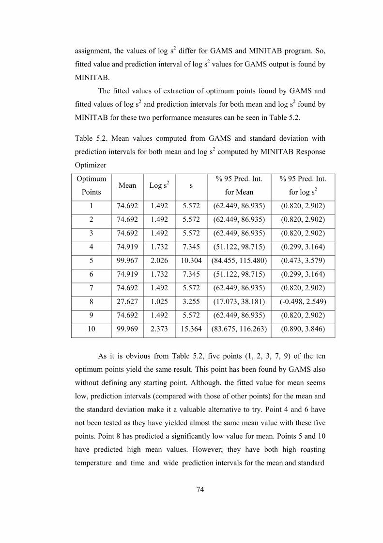
assignment, the values of log s2 differ for GAMS and MINITAB program. So,
fitted value and prediction interval of log s2 values for GAMS output is found by
MINITAB.
The fitted values of extraction of optimum points found by GAMS and
fitted values of log s2 and prediction intervals for both mean and log s2 found by
MINITAB for these two performance measures can be seen in Table 5.2. Table 5.2. Mean values computed from GAMS and standard deviation with
prediction intervals for both mean and log s2 computed by MINITAB Response
Optimizer
Optimum
Points Mean Log s2 s
% 95 Pred. Int.
for Mean
% 95 Pred. Int.
for log s2
1 74.692 1.492 5.572 (62.449, 86.935) (0.820, 2.902)
2 74.692 1.492 5.572 (62.449, 86.935) (0.820, 2.902)
3 74.692 1.492 5.572 (62.449, 86.935) (0.820, 2.902)
4 74.919 1.732 7.345 (51.122, 98.715) (0.299, 3.164)
5 99.967 2.026 10.304 (84.455, 115.480) (0.473, 3.579)
6 74.919 1.732 7.345 (51.122, 98.715) (0.299, 3.164)
7 74.692 1.492 5.572 (62.449, 86.935) (0.820, 2.902)
8 27.627 1.025 3.255 (17.073, 38.181) (-0.498, 2.549)
9 74.692 1.492 5.572 (62.449, 86.935) (0.820, 2.902)
10 99.969 2.373 15.364 (83.675, 116.263) (0.890, 3.846)
As it is obvious from Table 5.2, five points (1, 2, 3, 7, 9) of the ten
optimum points yield the same result. This point has been found by GAMS also
without defining any starting point. Although, the fitted value for mean seems
low, prediction intervals (compared with those of other points) for the mean and
the standard deviation make it a valuable alternative to try. Point 4 and 6 have
not been tested as they have yielded almost the same mean value with these five
points. Point 8 has predicted a significantly low value for mean. Points 5 and 10
have predicted high mean values. However; they have both high roasting
temperature and time and wide prediction intervals for the mean and standard
74

deviation. Therefore they have not been tried. So, the point where gypsum,
roasting temperature, roasting time, leach S/L ratio, leaching time and limestone
take the values of 2.787, 989, 30, 0.1, 120 and 2.512, respectively has been tried.
The results of the experiments yield the extraction values of %55.06 and
%50.00. These results are both less than the lower limit of the prediction interval
for the mean. The log s2 for these results is 1.107 which is inside the prediction
intervals for standard deviation.
So, this point has been modelled well with the regression for standard
deviation (but standard deviation has a wide gap) and could not have been
modelled by the regression model for the mean. It should have been said that
GAMS Non-linear programming could not predict the fitted values well for the
mean values. Moreover, it has been seen that modelling of standard deviation
with log s2 do not yield satisfactory results for GAMS. Apart from the misfit
problem, there has been no any improvement achieved for extraction of lithium
from boron clays.
5.3 Ridge Analysis
Ridge Analysis is the technique of steepest ascent applied to second
order surfaces.
It is worth to apply this technique to the regression model for the mean,
however, it is not possible to apply it to the model of log s2 as this model is a
third-order model. The idea of the model has been explained in Chapter II.
Therefore, the technique tries to solve the following equation;
(B- λI)x = -1/2 b
In our model,
A B C D E F A -10.02 0.0095 0.098 0 0 2.6 B 0.0095 -0.0015 -0.0006 -0.071 -0.00032 0.027 C 0.098 -0.0006 0 1.912 0 -0.0067D -0.75 -0.071 1.912 0 0 -1.484 E 0 -0.00032 0 0 0 0 F 2.6 0.027 -0.0067 -1.484 0 -3.49
75
B=

λ is an arbitrary value and the eigenvalues of B is denoted by δ.
The detailed formulation of the problem is given in the Appendix 5A.4.
The eigenvalues, δ , of the matrix B is found using MATLAB.
The eigenvalues are; -10.9511, -3.4231, -1.2753, -0.013, 0.0001, 2.1392.
So a GAMS program for solving the formulation of Ridge Analysis,
which comprises 6 equations, 2 inequalities and 7 unknowns, is proposed and
the code is given in Appendix 5A.5. The equations are;
(-10.02-λ)*A+0.0095*B+0.098*C+2.6*F= -9.095 [5.1]
0.0095*A-(0.0015+λ)*B-0.0006*C-0.071*D-0.00032*E+0.027*F=-1.443 [5.2]
0.098*A-0.0006*B-λ*C+1.912*D-0.0067*F=0.06045 [5.3]
-0.071*B+1.912*C-λ*D-1.484*F=54.105 [5.4]
-0.00032*B-λ*E=-0.3144 [5.5]
2.6*A+0.027*B-0.0067*C-1.484*D-(3.49+λ)*F=25.09 [5.6]
λ ≤ 2.1392 [5.7]
λ ≥ -10.9511 [5.8]
This is the program for finding the value of λ inside the region of
eigenvalues of matrix B. The solution of the program yields the values of 3.16,
983, 67, 0.187, 46, 2.6 and 0 for A, B, C, D, E, F and λ, respectively. According
to ridge analysis technique this point is a local optimum.
76
18.19 2.886
-0.1209 -108.21 0.6288 -50.18
I is the identity matrix,
b=
The formulation for finding the value of λ (so that location of the global
optimum) outside the region of eigenvalues of matrix B yield an infeasible
solution. That means ridge analysis could not propose a global optimum for this
model. The model and solution can be seen in Appendix 5A.6.
MINITAB has been used for finding the mean and standard deviation of
local optimum value proposed by Ridge Analysis. The fitted values and
prediction intervals for both performance measures are estimated by using
MINITAB. The fitted value for mean is 59.90 and prediction interval is (45.895,
73.898). The fitted value for standard deviation (log s2) is 1.587 and the
prediction interval is (0.216, 2.958). Although the prediction interval for
standard deviation is wide, prediction interval for mean makes this point a
candidate to be tried.
Therefore two experiments have been performed and the results are;
77.49% and 72,91%. The standard deviation (log s2) for these results is 1.021.
One of the results is just inside the prediction interval and the other is just
outside the prediction interval. Also, standard deviation is inside the prediction
interval. It can be concluded that the regression model fitted for mean and
standard deviation can predict the results of the Ridge Analysis well.
Apart from the adequacy of the regression model for this point, what is
more important is, an improvement in extraction of lithium has been achieved.
77.49% is the best result that has ever been obtained.
5.4 Optimization Outside the Response Surface
By changing the limits of the factors that have been introduced to the
GAMS non-linear program, it is possible to find out optimum points outside the
experimental region. Again the same algorithm of MINITAB Response
Optimizer and GAMS non-linear programming have been applied to outside the
experimental region. 10 optimum points have been computed by GAMS. As we
have been dealing with outside region, by nature the model could not be used to
predict the results of the experiment. However; it is decided to use GAMS and
77

the predicted results are found as 100 for the mean and less than 1.4 for log s2
that makes s being less than 5. While choosing the experiments to conduct,
another important criterion that has been considered is the economy of the
process. For example; roasting temperatures and leaching time have been chosen
as low as possible. 10 optimum points that have been computed by GAMS
outside the experimental region can be seen in Table 5.3.
Table 5.3. The optimum points found by GAMS outside the experimental region
Opt.
No A B C D E F s Mean
1 2.159 852 145 0.341 240 0.764 1.464 100
2 2.068 810 127 0.500 42 0.500 3.548 100
3 2.734 906 108 0.500 38 0.910 3.158 100
4 2.943 851 111 0.500 44 0.843 4.592 100
5 5.000 930 127 0.500 70 0.910 2.150 100
6 2.488 821 119 0.500 42 0.500 3.981 100
7 4.622 900 166 0.329 70 0.537 2.934 100
8 1.498 825 139 0.442 240 1.496 2.523 100
9 2.643 921 105 0.500 50 1.064 3.162 100
10 1.921 944 111 0.500 240 1.709 3.162 100
When we consider the economy of the process, the 2nd and 6th optimum
points seem to be the most economical processes as the roasting temperature is
low; as in the vicinity of 800°C, and leaching time is also low; just about 45
minutes. Therefore, 6th experiment has been conducted twice. However; the
results have been surprisingly low; 24.48% and 29.79%. As such a low values
are obtained for extraction of lithium from clays at very low temperatures, it has
been thought to make one more experiment with higher roasting temperatures.
From Table 5.3, the most suitable and relatively economic one is the 3rd
optimum point. Hence this point has been conducted twice.
78

The results have not been as low as those of the 6th point but they have
been far from being an global optimum for the extraction of lithium from boron
clays. The results have been 61.61% and 53.63%. These situations can be
observed for outside the experimental region, since the response surface may
change their shapes at another region.
79

CHAPTER VI
AN ATTEMPT TO IMPROVE THE OPTIMUM POINT
6.1. An Improved Experimental Design and Analysis
In Chapter 5, we have tried to model the mean and standard deviation of
extraction of lithium from boron clays. We have benefited from the response
surface modelling for achieving extraction as high as possible. However; except
for Ridge Analysis, no improvement can be made. Ridge Analysis has yielded
the results of 77.49% and 72.91%, which 77.49% is the highest value ever
obtained. However; the roasting temperature has been so high (around 980°C)
that extraction will not be economical. It is aimed in this chapter to get an
optimum with less cost.
Therefore, it has been thought to add the information obtained from the
optimum points tried to our response surfaces so that a new model can be set up.
Following this, a total of 6 points tried before have been appended to the
experimental layout (three of these have been found using MINITAB, and the
rest from ANOVA, GAMS Non-linear programming and Ridge Analysis).
Furthermore, one more point had been tried out of curiosity after investigating
the literature and experiencing the results of the experiments, the chemical
mechanism of roasting temperature and solubility equilibrium of leaching. At
this point, gypsum, roasting temperature, roasting time, leach S/L ratio, leach
time and limestone take the values of 1.5, 918°C, 120 min., 0.17, 120 min. and
1.5 respectively. Although the fitted value (22.58%) and the prediction interval
(-2.30, 47.47) of the regression model for the mean does not show good results,
this point had been tried. The results of the experiment have been 73.76% and
70.46%, which are higher values than many obtained so far except Ridge
Analysis results. Therefore, this point has been added to the response surface
modelling, as well. The seven points that have been treated as a part of the
80

experimental design and added to the model can be seen in Table 6.1.
Table 6.1 The points that have been added to the model
No Found from A B C D E F
1 GAMS 2.772 984 30 0.1 120 2.458
2 Ridge Analy. 3.178 986 67 0.187 33 2.6
3 MINITAB 4.5 850 120 0.4 120 1.5
4 MINITAB 1.5 987 30 0.1 120 1.5
5 MINITAB 1.5 878 120 0.36 120 1.5
6 ANOVA 4.5 950 120 0.2 120 1.5
7 Experience 1.5 918 120 0.17 120 1.5
These points have been appended in the experimental design. The model
for the mean extraction has been found after several attempts in order to satisfy
the assumptions for residuals. The best model that has been formulated with the
ANOVA table can be seen in Equation [6.1] and in Table 6.2. The starting
model can be seen in Appendix 6A.1.
µ = 769 + 78.2*A - 1.85*B - 1.38*C + 343*D - 9.46*E + 266*F + 0.0181*AB - 0.254*AC + 93.2*AD + 5.12*AF - 0.00115*BC
- 0.135*BD + 0.00819*BE - 0.297*BF + 9.09*CD + 0.0116*CE - 0.0124*CF - 4.09*DE - 0.584*EF - 17.4*A2 + 0.00114*B2 + + 0.00614*C2 – 1864*D2 + 0.0162*E2 + 8.23*F2 [6.1]
Table 6.2 ANOVA for Regression Analysis for model comprising optimum
points
Source dF Sum of Squares Mean Squares F p
Regression 25 16252.85 650.11 68.46 0.000
Residual Error 8 75.97 9.50
TOTAL 33 16328.83
R2 = 99.5% R2
(adj) = 98.1% S = 3.082
Durbin-Watson statistic = 1.96
81

The model has expectedly high value of R2(adj), and the Durbin-Watson
statistic shows no correlation between the residuals. p-value of the model is so
low that it can be concluded that this model is significant. The residuals versus
fitted values plot and the normal probability plot can be seen Figures 6.1 and
6.2, respectively.
Figure 6.1. The residuals versus fitted values plot for the regression
model [6.1] including optimum points.
Figure 6.2. The normal probability plot of residuals for the regression
model [6.1] including optimum points.
82
80706050403020100
3
2
1
0
-1
-2
-3
Fitted Value
Res
idua
l
3210-1-2-3
2
1
0
-1
-2
Nor
mal
Sco
re
Residual

Both plots show no violation of the assumptions made for residuals.
Residual versus fitted values plot shows that the variance of the residuals is
constant. Normal probability plot resembles a straight line leading in a
conclusion for normal distribution of residuals.
The β significance table of the parameters can be seen in Table 6.3.
83

Table 6.3. Significance of β terms of the model [6.1] including optimum points Predictor Coefficient Standard Error T p
Constant 768.8 332.8 2.31 0.050
A 78.16 13.52 5.78 0.000
B -1.8507 0.7148 -2.59 0.032
C -1.3787 0.4912 -2.81 0.023
D 342.71 72.37 4.74 0.001
E -9.458 1.507 -6.28 0.000
F 266.01 42.32 6.29 0.000
A*B 0.018113 0.006303 2.87 0.021
A*C -0.25436 0.05986 -4.25 0.003
A*D 93.18 20.50 4.55 0.002
A*F 5.1191 0.4145 12.35 0.000
B*C -0.0011513 0.0002031 -5.67 0.000
B*D -0.13523 0.06076 -2.23 0.057
B*E 0.008193 0.001166 7.03 0.000
B*F -0.29740 0.04633 -6.42 0.000
C*D 9.0914 0.8654 10.51 0.000
C*E 0.011571 0.001322 8.75 0.000
C*F -0.01238 0.01421 -0.87 0.409
D*E -4.0865 0.7233 -5.65 0.000
E*F -0.58447 0.08325 -7.02 0.000
A2 -17.383 2.087 -8.33 0.000
B2 0.0011381 0.0003914 2.91 0.020
C2 0.006138 0.003136 1.96 0.086
D2 -1863.7 225.5 -8.27 0.000
E2 0.016426 0.002986 5.44 0.001
F2 8.235 1.666 4.94 0.001
84

The β significance table has implied that every term has a p-value of at
most 10% except roasting time and limestone interaction factor. However;
excluding this term from the model makes it worse in the manner that Durbin-
Watson statistic shows a positive correlation. The model with no factor having
p-value higher than 10% and the sum of squares of the best model can be seen in
Appendix 6A.2 and 6A.3. Therefore this model is thought to be the best
regression model that comprises optimum points for mean.
At this point, it will be beneficial to look for log s2 model. The
formulation and the ANOVA of the log s2 model can be seen below.
Log s2 = 386 - 2.40*A - 0.979*B + 0.441*C + 309*D - 1.48*E + 63.8*F
-0.0762*AC + 28.9*AD + 0.240*AE -0.000081*BC + 0.00180*BE -0.0697*BF + 3.12*CD - 0.00450*CE - 3.66*DE - 0.117*EF - 4.17*A2 +0.000546*B2 – 536*D2 + 0.00134*E2 + 2.16*F2 [6.2]
Table 6.4. ANOVA for Regression Analysis for model of log s2 comprising
optimum points
Source dF Sum of Squares Mean Squares F p
Regression 21 36.8068 1.7527 3.26 0.019
Residual Error 12 6.4433 0.5369
TOTAL 33 43.2501
R2 = 85.1% R2(adj) = 59.0% S = 0.7328
Durbin-Watson statistic = 2.07
The Durbin-Watson statistic of the model shows no correlation between
the residuals. R2 value is 85.1% and R2(adj) value is 59% which is low value.
Moreover, the gap between the values of R2 and R2(adj) is wide. This means that
we have some unnecessary terms in our model. However; trying to decrease the
number of factors in the model do not improve the adequacy of the model so that
this model has been chosen as the best model for log s2 with the optimum points
included. The residuals versus fitted values and normal probability plot have
implied that the assumptions made about the residuals are satisfied. The plots
85

and the β significance test of the factors can be seen in the following pages.
Figure 6.3. The residual versus fitted values plot for the regression model of log
s2 [6.2] including optimum points
Figure 6.4. The normal probability plot of residuals for the regression
model of log s2 [6.2] including optimum points
86
3210-1-2-3
1
0
-1
Fitted Value
Res
idua
l
-1 0 1
-2
-1
0
1
2
Nor
mal
Sco
re
Residual

Table 6.5. Significance of β terms of the regression model [6.2] including optimum points for log s2
Predictor Coefficient Standard Error T p
Constant 386.3 100.0 3.86 0.002
A -2.397 2.581 -0.93 0.371
B -0.9791 0.2496 -3.92 0.002
C 0.4412 0.1380 3.20 0.008
D 308.64 86.16 3.58 0.004
E -1.4801 0.3342 -4.43 0.001
F 63.80 15.63 4.08 0.002
A*C -0.07619 0.2346 -3.25 0.007
A*D 28.917 7.496 3.86 0.002
A*E 0.23968 0.06506 3.68 0.003
B*C -0.00008124 0.00004605 -1.76 0.103
B*E 0.0018038 0.0004253 4.24 0.001
B*F -0.06965 0.01727 -4.03 0.002
C*D 3.1239 0.8306 3.76 0.003
C*E -0.004496 0.001396 -3.22 0.007
D*E -3.6604 0.9857 -3.71 0.003
E*F -0.11725 0.03032 -3.87 0.002
A2 -4.168 1.043 -4.00 0.002
B2 0.0005459 0.0001381 3.95 0.002
D2 -536.4 144.3 -3.72 0.003
E2 0.0013444 0.0003905 3.44 0.005
F2 2.1556 0.5963 3.61 0.004
Modelling of log s2 with optimum points included could not have been
modelled adequately. However; this model is simpler than the previous one.
87

MINITAB Response Optimizer is used to obtain new optimal points.
and see if both models could predict the results of the experiment. Fortunately,
as log s2 have been modelled with addition of quadratic terms, it is now possible
to make a dual approach to the optimization using MINITAB. In other words, In
MINITAB Response Optimizer we can define limits for both the mean and log
s2 and require an optimum point that will maximize extraction with minimum
variation. Therefore, for mean a minimum value of 70 and a target value of 100
whereas for log s2, a maximum value of 1.6 (s will be 6.31 then) and a target
value of 1 (s will be 3.162 then) have been defined as limits for MINITAB
Response Optimizer. Same algorithm with the one that has been applied in the
previous chapters has been applied. The Optimizer has found 10 points. The
starting and optimum points can be seen in Appendix 6A.4 and the mean and the
log s2 values with the prediction interval for both measures can be seen in Table
6.6.
Table 6.6. The prediction intervals for the mean and the standard deviation
computed by MINITAB Response Optimizer that use models [6.1] and [6.2]
Optimum
Points Mean Log s2 s
% 95 Pred. Int.
for Mean
% 95 Pred. Int.
for log s2
1 71.930 0.669 2.160 (61.908, 81.953) (-1.572, 2.910)
2 80.423 1.640 6.607 (69.620, 91.226) (-0.703, 3.982)
3 74.437 0.999 3.159 (64.067, 84.807) (-1.234, 3.233)
4 84.229 5.427 517.01 (73.729, 94.730) (1.510, 9.343)
5 63.522 2.059 10.703 (53.701, 73.343) (-0.561, 4.678)
6 94.599 6.367 1525.81 (82.016, 107.182) (2.209, 10.526)
7 123.874 -10.646 4.8x10⁻⁶ (75.216, 172.532) (-23.273, 1.982)
8 95.439 1.387 4.937 (80.563, 110.314) (-1.393, 4.167)
9 125.099 15.432 5.2x10⁷ (99.660, 150.538) (7.622, 23.201)
10 86.509 0.892 2.793 (75.316, 97.702) (-1.557, 3.341)
88

From Table 6.6, it can be seen that standard deviation has a wide gap for
most of the points. The smallest standard deviation are obtained at points 1 and
10 which we have already tested (point 10 is approximately the same as the
point found by Ridge Analysis and point 1 has earlier been found by intuition).
Log s2 for points 10 and 1 are 1.021 and 0.736, respectively. They are both in
the prediction interval for log s2. However; recall that the mean extraction results
obtained from these two experiments have not been satisfactorily and
economically high (highest value for point 10 is 77.49%, and for point 1 is
73.76%). Hence, it is decided to look for a point to get higher mean extraction
values more economically at the expense of standard deviation. Undesirability of
low roasting temperatures has eliminated points 3, 8, 9, 2 and 6. Point 7 has been
found without defining any starting point and it is shown here for illustrative
purposes. Also experiences about the extraction mechanism has shown that
roasting temperatures about 850°C result in low yields. Hence we are left with
only two alternatives; points 4 and 5. Although point 5 has a narrower prediction
interval for log s2, point 4 has predicted mean extraction values much higher
with a narrower prediction interval. Therefore it is decided to conduct
experiments for point 4. Gypsum, roasting temperatures, roasting time, leach
solid to liquid ratio, leaching time and limestone take the values of 1.5, 915, 120,
0.26, 120 and 1.5, respectively.
At first, two experiments have been conducted for this point and the
results have been: 74.87 and 83.01%. The standard deviation of these two
experiments is 5.756 (log s2 is 1.520) which is an acceptable value. More
importantly both of the results have been between the prediction interval limits
for the mean. Also 83.01% is the largest extraction value of lithium from boron
clays obtained experimentally. Hence we have conducted 4 more repetitions at
this point to assure the persistence of these results and the results are; 83.84%,
85.54%, 86.39% and 89.22%. All of them are in the prediction interval (73.729,
94.730) for the mean and they are the highest that have been achieved so far.
The mean of all these six experiments is 83.81% and the standard deviation is
89

4.888. (log s2 is 1.378) which is still an acceptable value although it is outside
the prediction interval (1.510, 9.343) for log s2 .From these 6 experiments, the
lowest 3 mean values (74.87%, 83.01%, 83.84%) and the highest 3 mean values
(85.54%, 86.39%, 89.22%) have been grouped with each other and Signal-to-
Noise ratios have been calculated. For the lower group, S/N ratio is 38.097 and
for the higher group, 38.794. They are much better than the ANOVA results. As
a result, it can be concluded that the model for the means including the optimum
points has successfully found the optimum (or a highly desirable point) and can
predict the results well. The model is adequate at that point.
Gaining knowledge from these experiments and examining the literature
has led us to think of an experiment at increased time of roasting and leaching
and beyond the experimental region. For this purpose, point 7 of Table 6.1 has
been used. Only roasting leaching time has been altered. Firstly the experiments
have been performed at 120 minutes of roasting time and 180 minutes of
leaching time. The results that have been obtained were 82,89% and 82.22%,
(log s2 is –0.649) which are not significantly different from the optimum point,
that have been found from model including the optimum points.
Furthermore as a last experiment, increasing of roasting and leaching
time by 60 minutes have been thought. The results of the experiment show
values of 86.70% and 93.53% (log s2 is 1.368). These results have been the
highest of all experiments that have been conducted and log s2 is an acceptable
value. However; as the roasting and leaching time prolonged by a significant
value, the comparison of economic value of these results and the optimum point,
found by the model including the local optima, should be considered.
As a result, this study can claim that in the experimental region at least
74.87% and at most 89.22% (both are in the prediction interval) mean extraction
has been achieved with an acceptable standard deviation. The points that would
yield this result with an economical process should be 1.5, 915°C, 120, 0.26, 120
and 1.5 for gypsum, roasting temperature, roasting time, leach solid to liquid
ratio, leaching time and limestone, respectively. Higher extraction values can be
achieved but increasing roasting and leaching time will affect the economy of
the process significantly.
90

For illustrative purposes, contour plots of roasting temperature versus
leaching solid to liquid ratio drawn for both the mean and log s2 can be seen
from Figures 6.5 and 6.6.
Figure 6.5. Contour plot of roasting temperature versus leaching solid to
liquid ratio for mean
Figure 6.6. Contour plot of roasting temperature versus leaching solid to
liquid ratio for log s2
91
20 40 60 80 90 100
850 950 1050
0.1
0.2
0.3
0.4
Ro. Te. (°C)
Leac
h S
/L R
atio
Hold values: Gypsum: 1.5, Ro.Ti.: 120.0, Leach Ti.: 120.0, Limestone: 1.5
Optimum
-2 -1 0 1 2
850 950 1050
0.1
0.2
0.3
0.4
Ro. Te. (°C)
Leac
h S
/L R
atio
Hold values: Gypsum: 1.5, Ro.Ti: 120, Leach Ti.: 120, Limestone: 1.5
Optimum

6.2. Comparison of Results to Relevant Literature Work
There are some studies that have tried to extract lithium from clays.
These studies have been pointed out in Chapter II. From these, the most
important and the relevant ones are Mordoğan et. al. (1995), Beşkardeş et. al.
(1992) and Lien (1985). Mordoğan et. al. (1995) and Beşkardeş et. al (1992)
have studied the boron clays whereas Lien (1985) has studied montmorillonite
type clay which does not contain boron. The optimum points that have been
found by these studies and the economic analysis of them can be seen in Table
6.7. Crocker et. al. (1988) is a modification of the study of Lien (1985) in order
to decrease the cost of the process by decreasing the raw materials.
Table 6.7. Comparison of Results to Other Studies
This
Study
Mordoğan
1995
Beşkardeş
1992
Crocker
1988
Field Bigadiç Kırka Bigadiç Nevada
Lithium Content (ppm) 2000 2800 2007 6000
Optimum Points
Clay 5 5 5 5
Gypsum 1.5 0.834 1.5 2
Roasting Temp. (°C) 915 900 850 900
Roasting Time (min.) 120 120 120 120
Leaching S/L Ratio 0.26 0.1 0.5 0.665
Leaching Time (min.) 120 60 ---- 5
Limestone 1.5 0 1.5 2
Performance Measures
Average Extraction (%) 83.81 77.00 72.78 84.00
Cost ($/kg Li2CO3) 6.91 ---- 10.65 4.45
Standard Deviation 4.89 ---- ---- ----
As it is seen from Table 6.7, the optimum point found in this study is somewhat
92

similar to those of the other studies, although in this study natural and waste raw
materials are used, which reduces cost and saves the environment.
The extraction values achieved in this study are the highest for boron
clays and nearly the same with those of Crocker et. al. (1988). Mordoğan et. al.
(1995) have studied Kırka clays which has a different composition than Bigadiç
clays so they do not need to use limestone. The main difference of this study
from other studies is high leaching time, however, it is seen from Figure 4.6 that
30 minutes of leaching time can be enough for high extraction. A confirmation
experiment has been done for decreasing leaching time (other points remaining
the same) and has resulted in about 80% extraction. Further experiments are still
being conducted. Another important factor is leaching solid to liquid ratio which
is high for this study compared to Beşkardeş et. al. (1992) and Crocker et. al.
(1988). This factor is important in the sense that high liquid amount needs more
water to evaporate and this in turn increases the cost significantly. Experiments
are still being conducted in order to increase the solid to liquid ratio. The
author’s opinion is that there will not be high differences in the extraction values
for that factor.
The cost of producing lithium carbonate from clays is lowest for
Crocker et. al’s (1988) study but this is mainly due to the higher lithium content
of the clay used in that study. The detailed cost analysis made for this study by
a similar approach with Crocker et. al (1988) is given in Chapter VII.
Only this study has focused on variation of the extraction results. This
performance measure has not been considered in the other studies. An
acceptable standard deviation (4.89) has been achieved in this study.
93

CHAPTER VII
ECONOMIC IMPACT AND ANALYSIS OF THE STUDY
This study aims to design the extraction process so that high extraction
results are achieved without costly control on noise factors. Here, major savings
come from the use of limestone directly from the nature and gypsum as a waste
product of boric acid production. In traditional practice, to achieve high lithium
extraction results reagent grade raw materials are used which add further cost to
process. Hence, we have made a cost analysis in order to see overall savings
resulted from this study. In this analysis we have used the study of Crocker et.
al. (1988) for comparison. The results of the annual operating cost analysis are
summarized in Table 7.1.
It has been intended to develop a rough cost estimate assuming the worst
case and the cost analysis is done based on processing 1000 tons/day. According
to Crocker et. al. (1988) clay:gypsum:limestone ratio is 5:2:2, however we have
found the optimum ratio as 5:1.5:5:1.5. Therefore, in Crocker et. al. (1988)
about 1900 tons/day of raw materials can be processed, while we can process
about 1600 tons/day of raw materials. Furthermore, some cost figures such as
those for depreciation, taxes, insurance, balls, chemicals, and process water for
our case have been found simply by adjusting the corresponding Crocker et. al.
(1988) figures by the capacity (i.e. by multiplying them by 1600/1900).
Evaporation and leaching costs have been taken as the same.
94

Table 7.1. Comparison of operating cost of the proposed lithium extraction
process to that of Crocker et. al. (1988)
Crocker et. al. (1988), $ This study, $ Annual kg Li2CO3 Annual kg Li2CO3 Lithium content (ppm) 6000 2000 I. Direct Costs A. Raw Materials Clay 0 0.000 0 0.000 Limestone 3.395.700 0.437 0 0.000 Gypsum 3.326.400 0.428 1.414.000 0.514 Soda Ash 2.313.000 0.297 936.000 0.342 Balls 122.300 0.015 103.000 0.037 Chemicals 3.600 0.002 3.000 0.001 Total 9.161.000 1.179 2.456.000 0.894 B. Utilities Electric Power 1.190.600 0.152 1.920.000 0.698 Process Water 63.000 0.009 53.000 0.019 Fuel 8.240.100 1.057 6.294.000 2.289 Total 9.493.700 1.218 8.267.000 3.006 C. Direct Labor Labor 1.437.100 0.186 189.000 0.069 Supervision 215.600 0.029 28.000 0.010 Total 1.652.700 0.215 217.000 0.079 D. Maintenance Labor 1.437.100 0.218 224.000 0.081 Supervision 340.000 0.045 45.000 0.016 Materials 1.700.100 0.218 1.432.000 0.521 Total 3.740.100 0.471 1.701.000 0.619 E. Payroll Overhead 1.292.400 0.166 170.000 0.062 F. Operating Supplies 748.000 0.098 340.000 0.124 TOTAL DIRECT COST 26.087.900 3.347 13.151.000 4.782 II. Indirect Costs 2.157.100 0.278 767.000 0.279 III. Fixed Costs Taxes 811.400 0.105 684.000 0.249 Insurance 811.400 0.105 684.000 0.249 Depreciation, 20 yr 4.755.500 0.612 4.005.000 1.456
TOTAL PRODUCTION COST 34.623.300 4.45 19.291.000 7.014
Annual Production (ton) 7785 2750
Waste Reducing Gain ----- ----- -1.200.000 -0.436 TOTAL
PRODUCTION COST 34.623.300 4.45 18.091.000 6.578
95
In Crocker et. al. (1988), unit cost of electricity is taken as 0.047 $/kW.h,
however, for Turkey unit cost of electricity is assumed as 0.09 $/kW.h. Crocker
et. al. (1988) have used heavy oil for fuel (0.85 $/gal and 1 gallon gives 153.000
Btu of heat) and we have used natural gas as the fuel (0.02 $/1000 kcal). Labor
cost is 11.75 $/hr in Crocker et. al. (1988) and we have taken the labor cost as
13.500 $/annual per person on the average.
Some cost figures seem to be higher with respect to unit cost of Li2CO3.
This is due to the fact that in our study annual production of Li2CO3 is about
three times less than Crocker et. al. (1988) study as the lithium content of
Bigadiç clays is much lower (2000 ppm) than that of Crocker et. Al. (1988)
study (6000 ppm).
Although it is intended to develop an estimate for the worst case,
evaporation cost (that will be added to fuel part) has been taken as the same as
that of Crocker et. al (1988) study, although we have higher water amount to
evaporate, hence higher cost.
Some cost figures such as those for gypsum and waste reducing gain can
not be displayed here as they are confidential for Eti Holding. Waste reducing
gain has been estimated assuming that the leaching residue will find an
application area. This point is discussed in detail later both in this section and in
Chapter 8.
The operating cost of Li2CO3 from boron clays that contain 2000 ppm
lithium has been estimated as 6.578 $/kg whereas, the same figure for Crocker
et. al. (1988) study is 4.45 $/kg. On the other hand, if the study done by Crocker
et. al (1988) had lithium content of 2000 ppm in their clays, then the operating
cost would roughly be around 13.35$/kg. In this study, the ratio of raw materials
to clay has been decreased and also the raw materials that will not bring any
additional cost to Eti Holding, Inc have been used. This has brought about 50%
savings in the operating cost. However; when we consider the import price of
Li2CO3 in Turkey in year 2002 (3.98$/kg) this process is not be preferable as of
the current time. If the selling price of Li2CO3 in the world market is about
3.5$/kg, then, in order for this process to be preferable Bigadiç clays should
contain around 3500 ppm lithium, or Li2CO3 selling price should increase to
96
about 6 $/kg.
Another important point to consider is the application of the residue of
the leaching process. This residue is a waste in this study, however, by changing
the amounts of raw materials (hence probably decreasing extraction yield) this
residue can be used in other industries. This adjustment will bring additional
cost reduction to process. An economic off-set should be made with the possible
usage of the residue and extraction percentage. Moreover, possible application
of the leaching residue will result in a significant benefit to society such as
decreasing further the solid wastes to environment. In case that this residue is
not used, about 30% waste reduction can been achieved at the optimal settings.
While making the cost analysis, natural gas has been used as the fuel
source and it is seen that it has added about 35% cost to the process. Decreasing
the cost of fuel as well as the cost of electricity (about 10% cost to the process)
will bring significant cost improvements. Also pelletizing has been added in the
cost analysis. However; a pilot scale study should be conducted to decide
whether pelletizing is necessary or not.
The price of Li2CO3 has increased about 5-10% in year 2001 and it is
predicted that the price will increase in the following years. So the price trend of
Li2CO3 should be followed to determine when the proposed extraction process
need to be put in action.
In addition to all these, the amount and grade of lithium reserves of
boron clays (especially Bigadiç clays) should be determined and if a field
containing about 3000 ppm lithium is found, it should be stored in a separate
place. An estimation of process cost in that case might indicate that extracting
lithium locally using the proposed approach is more economical than importing
it.
97

CHAPTER VIII
CONCLUSION AND SUGGESTIONS FOR FUTURE WORK
In mining industry, it has not been straightforward to make a
standardization as the industry strongly depends on natural factors. In this study,
a methodology has been demonstrated for achieving the desired result (lithium
extraction) independent of the grade of the raw materials that has been input. All
the raw materials have been chosen as they are solid wastes from production
facilities or gangue minerals. In other words, the need for standardization is
sought to be reduced. This study specifically has been concentrated on the
extraction of lithium from boron clays by using a solid waste of boric acid
production, gypsum and a calcium carbonate rich field in boron mines that could
not been utilized, otherwise.
In this study, evaluation of optimum extraction of lithium from boron
clays has been examined. The procedure has been based on two main
performance measures; mean of extraction and the standard deviation of the
extraction values. Statistical experimental design principles more specifically
orthogonal arrays have been used in such a study for the first time to the best of
our knowledge.
The objective of robust extraction of lithium is to find optimal settings of
parameters which produce the maximum extraction with minimum variation
around this maximum.
In this study, guidelines for the conduct of experiments have been
developed and data collection and transformation methods have been presented.
Data analysis has been performed for modelling both the mean and the
standard deviation. A methodology called S/N transformation comprising both
of these performance measures has been utilized.
98

While seeking to reach the optimum settings of parameters, 4 different
optimization algorithms have been used. These are ANOVA, Regression
modelling, Non-linear programming, and response surface methods applied to
second-order surfaces, Ridge Analysis. A widely used method of robust design,
ANOVA, has been performed by making Signal-to-Noise ratio transformation of
data. The results obtained from ANOVA do not yield satisfactory extraction
values. The reason for this lack of achieving may be two fold; ANOVA has
taken only the linear terms into consideration, and we are confined to only the
experimental levels of the factors for the optimum.
Modelling through regression has been separated into two parts. The
mean and the standard deviation has been modelled. MINITAB 13.3 package
program has been used for modelling. Mean has been modelled with high values
of adjusted multiple coefficient of determination R2(adj). Also the assumptions
about the residuals for mean has been met satisfactorily. No correlation has been
observed for errors. Prediction intervals for mean mostly have been narrow
enough. The standard deviation could not be modelled as adequately as the
mean. Although residuals confirm all assumptions and no correlations have been
observed between them, there has been a wide gap between multiple coefficient
of determination (R2) and adjusted multiple coefficient of determination (R2(adj)).
Prediction intervals for the standard deviation have been too wide. The
confirmation experiments for regression modelling have shown variability
among different points for both the mean and the standard deviation. However;
an improvement from the experimental results obtained could not be achieved
by the tested optimal points. For this case, a further modelling have been tried
and this modelling is based on the addition of optimal points to the first model.
This model has shown an adequate fit to the mean whereas standard deviation
still could not be modelled as adequately as the mean. There are several reasons
for this lack of fit. One and the most important reason is that the raw materials
used for this study have been chosen from nature as they are and have not been
processed for standardization before beginning of the tests.
99

Especially, limestone CaCO3 content has shown a significant variability.
The model that has treated the optimal points as a part of experimental design
has concluded in an extraction of lithium that has been the highest of all tests.
Also the standard deviation at these optimal settings is found experimentally to
be acceptable although it could not be predicted by the model of the standard
deviation.
Another optimization tool that has been tried in this study is Non-linear
programming. Dual responses have been tried to be solved for this purpose;
maximization of the mean of extraction of lithium and minimization of the
standard deviation around the mean. Non-linear programming has been made by
using GAMS software. The results obtained from this study has yielded sub-
optimal points which have not shown a significant improvement of the
experimentally obtained results. Also by incorporating the non-linear
optimization technique, some points outside the experimental region that can
lead to the desired results have been found. While computing these points,
economic considerations have been considered and the points that might bring
cost reduction have been tried. However; satisfactory extraction values could not
be achieved, either.
The last optimization algorithm that has been used in this study is the
method that has been applied to second-order surfaces of response surface
methodology, Ridge Analysis. This method has comprised some matrix algebra
and MATLAB package program has been used for solving the equations. Ridge
Analysis have predicted the results of the experiment for both performance
measures satisfactorily. Moreover, it has yielded an optimum value that has
been higher than the previous results of the experimental region. However; this
optimum point could not be treated as the global optimum as the algorithm
suggests that it is a local optimum. Furthermore, this optimum point has a
drawback that the roasting temperature is very high at this point.
An economic off-set should be calculated for other factors. As the
roasting process is a reversible process, less time is needed for completion of
converting process for higher temperatures than for lower temperatures. So for
100
deciding on optimal settings, this study has presented two solutions. If lower
roasting temperature will be more suitable, then the result obtained from
modelling of the mean by adding optimum points to the experimental region
should be used. The settings for this optimum are 1.5, 915°C, 120 minutes, 0.26,
120 minutes and 1.5 for gypsum, roasting temperature, roasting time, leaching
solid to liquid ratio, leaching time and limestone, respectively. If less time of
roasting time will be seen more adequate for extraction, the results obtained
from Ridge Analysis, should be used. The settings for the parameters are 3.178,
986°C, 67 minutes, 0.187, 33 minutes, 2.6 for the same order of factors.
Extraction of lithium from boron clays has had a solid waste at the end of
the leaching process. The raw materials other than the lithium containing clay
must be chosen for evaluation of this solid waste. This study is unique in the
sense that natural limestone has been used as CaCO3 source and waste product
of boric acid is used as gypsum source. These two raw materials will not bring
any additional cost to the extraction process as they are owned by Eti Holding,
Inc. Moreover, using these wastes will decrease the need hence cost for storing
them. Therefore, an important parameter to consider here is the amount of
limestone and gypsum used in lithium extraction. As another solid waste has
obtained during the extraction process, the optimal settings for raw materials can
be modified in a way to utilise that solid waste. For this purpose, pelletizing can
be introduced to the process. The author’s opinion is that it will be crucial to
make a study for utilising the solid waste of lithium extraction in order to
decrease the economy of the process significantly.
In this study, experiments have been made based on clay amount. 40
grams of clay have been used and gypsum and limestone ratio have been chosen
with respect to that value. For example, at the optimal settings, gypsum/clay
ratio and limestone/clay ratio are both 1.5/5 meaning that 12 grams of gypsum
and limestone have been used. This will add to totally 64 grams. After the
leaching process, about 45 grams of solid waste are left. This means that at the
optimal settings about 30% reduction can be achieved for the wastes. Moreover,
by just using natural raw materials, about 78% cost reduction for extraction have
101

been gained compared with the study made by Crocket et. al. (1988). To add up,
this study not only extracts lithium in an economic way but also attempts to
decrease the solid wastes of Eti Holding, Inc.
The results of the cost analysis show that if import price of lithium
increases more than 50%, if we find enough clays that contain about 3500 ppm
lithium and if fuel and electricity prices decrease, then it is economically
feasible and more advantageous for Turkey to produce its own lithium (and
export the excess) by using the proposed extraction process. Apart from the cost
considerations, this proposed process has a social benefit to the society in the
manner that the solid wastes to the nature are decreased by significantly.
Another important research that should follow this study is the
precipitation of lithium. Lithium carbonate is the most widely used compound of
lithium and the studies in literature (Lien, 1985, Beşkardeş, 1992) have been
concentrated on it. The optimal settings for the precipitation of lithium can be
found by following a similar approach.
It has been well known to the researchers of robust design that tolerance
design should have been performed after robust design. This study needs to be
followed by a tolerance design study as the raw materials used in extracting
lithium are all solid wastes and they show great variability (especially limestone)
in their beneficial portion for extraction of lithium. In such a study, the
allowable variation for lithium content of clay, limestone’s CaCO3 content and
gypsum’s CaSO4.2H2O content or lower limits of lithium content of the clays,
calcium carbonate (CaCO3) content of limestone and calcium sulphate dihydrate
content (CaSO4.2H2O) of gypsum can be defined for optimum extraction of
lithium from boron clays with much smaller variation than the variation obtained
in this study. This will further reduce variation of the results. As a part of the
tolerance design, a detailed cost analysis should be conducted for producing
lithium carbonate or any other lithium compound. In order to make the cost
analysis more accurately, the grade and reserves of lithium content of boron
clays should have been determined.
102

LIST OF REFERENCES
[1] Abacıoğlu U., “Design of Water Triple Point Cells Using Statistical Experimental Design Techniques”, M.S.Thesis, Boğaziçi University, Chemical Engineering Department, 1999
[2] Beşkardeş O., Bayhan H., Ersayın S., “Investigation and Evaluation of Lithium Potentials in Bigadiç Clays”, Hacettepe University, Ocak 1992 [3] Box G. E. P., Draper N. R., “Empirical Model-Building and Response
Surfaces”, John Wiley & Sons, Inc., 1987, pg. 375-381 [4] Box G. E. P., Wilson K. B., “On the Experimental Attainment of Optimum
Conditions”, J. Roy. Statist. Soc., B13, 1-38, discussion 38-45, 1951 [5] Büyükburç A., Maraşlıoğlu D., Bilici U., Gündüz M., “The Determination and Evaluation of Lithium Contents of Boron Ores and Clays”, Eti Holding Co. R&D Department, July 2002
[6] Coad M., “Lithium Production in Chile’s Salar de Atacama”, Industrial Minerals, October 1984, pg. 27-33 [7] Crocker L., Lien R.H., and Others, “Lithium and Its Recovery From Low
Grade Nevada Clays”, U.S. Bureau of Mines Report of Investigations No:8832, 1988
[8] Davidson C. F., “Recovery of Lithium From Clay by Selective
Chlorination”, U.S. Bureau of Mines Report of Investigations No:8523, 1981
[9] Edlund V. E., “Lime-Gypsum Processing of McDermitt Clay for Lithium
Recovery”, U.S. Bureau of Mines Report of Investigations No:8832, 1983
103
[10] Erdoğan K., “Linking of Axiomatic Design and Robust Design Methodologies Through Information Content in Design” M.S.Thesis, T.C.Marmara University, Mechanical Engineering Department, 2000 [11] Fishwick J. H.,”Application of Lithium in Ceramics”, Cahners Publishing
Company, Inc., 1974 [12] George C. T., Soran B., William H. J., Daniel P., Stigler M. S., (Editors) “Box on Quality and Discovery with Design Control and Robustness”, Wiley Series, 2000, pg. 146-169 [13] Handle B., Broderick G., Paschen P., “A Statistical Response Surface Study of the Tellurium Electrowinning Process”, Hydrometallurgy, Vol.46, pg.105-120, 1997
[14] Hoerl A. E., “Optimum Solution of Many Variables Equations”, Chem. Eng. Prog., Vol.55, pg.69-78, 1959
[15] Hoerl R. W., “Ridge Analysis 25 Years Later”, Am. Statistics, Vol. 39, pg.186-192, 1985
[16] Khoei A. R., Masters I., Gethin D. T., “Design Optimization of Aluminium Recycling Processes Using Taguchi Technique”, Journal of Materials Processing Technology, v.127, pg.96-196, 2002
[17] Koolen J. L. A., “Simple and Robust Design of Chemical Plants”, Computers and Chemical Engineering, 1998, Vol.22, Suppl., pg. S255-S262 [18] Köksal G., “Robust Design of Batch Dyeing Process”, Ph.D.Thesis, North
Carolina University, Department of Industrial Engineering, 1992 [19] Köksal G., Smith A. W., Fathi Y., Lu J. C., McGregor R., “A case study in
off-line quality control: characterization and optimization of batch dyeing process design”, International Journal of Technology Management, Vol.16, Nos.4/5/6, 1998, pg. 358-382
104

[20] Kroschwitz I. J. (Executive Editor) and Grant H. M. (Editor), “Kirk-Othmer Encylopedia of Chemical Technology”, Vol. 15, “Lithium and Lithium Compounds”, pg. 434-463, 1994
[21] Lien R. H., “Recovery of Lithium From a Montmorillonite-Type Clay”,
U.S. Bureau of Mines Report of Investigations No:8967, 1985 [22] Lin K. J. D., Tu W., “Dual Response Surface Optimization” Journal of
Quality Technology, Vol.27, No.1, January 1995, pg.34-39 [23] May J. T., Witsowsky D. S., Siedel D. C., ”Extracting Lithium From Clays
by Roast-Leach Treatment”, U.S. Bureau of Mines Report of Investigations No: 8432, 1980
[24] Mendenhall W., Sincich T., “A Second Course in Statistics: Regression
Analysis”, Prentice-Hall, Inc., pg.825-826, 1996 [25] Menon R., Tong L. H., Zhijie L., Ibrahim Y., “Robust Design of a Spindle
Motor: A Case Study”, Reliability Engineering and System Safety, vol.75, pg.313-319, 2002
[26] Montgomery D. C., “Introduction to Statistical Quality Control”, John
Wiley & Sons, Inc., 1997, pg. 572-582 [27] Mordoğan H., Helvacı C., Malayoğlu U., “The Existence and Evaluation
Possibilities of Lithium in Boron Clays and Lakes”, Industrial Raw Materials Symposium, Izmir, 1995, pg. 185-196
[28] Myers H. R. “Response Surface Methodology”, Allyn and Bacon, Inc.,
1971 [29] Myers H. R., “Response Surface Methodology-Current Status and Future Directions”, Journal of Quality Technology, Vol.31, No.1, January 1999, pg. 30-43
105

[30] Myers H. R., Khuri I. A., Carter Jr. W. H., “Response Surface Methodology: 1966-1988”, Technometrics, May 1989, Vol.31, No.2, pg. 137-157
[31] Ober J. A., “Lithium” United States Geological Survey Minerals
Yearbook, 2001 [32] Ooi K., Miyai Y., Katoh S., “Recovery of Lithium From Seawater by Manganese Oxide Absorbent”, Separation Science and Technology, Vol. 21, No.8, 1986, pg. 755-766 [33] Özler C., “An Investigation of Response Surface Methodologies for Aiming
At Process Improvement”, M.S.Thesis, T.C. Dokuz Eylül University, 1997 [34] Phadke M. S., “Quality Engineering Using Robust Design”, Prentice Hall PTR, 1989 [35] Ross J. P., “Taguchi Techniques for Quality Engineering”, McGraw Hill, Inc., 1988 [36] Saller M., O’Driscoll M., ”Lithium takes charge, Supply & Demand
Reviewed”, Industrial Minerals, March 2000, pg. 37-47
[37] Ünal A. Y., “Application of Taguchi Method to the Process Parameters of Gear Box Access Rod Production”, M.S.Thesis, T.C. Marmara University, 2001
106

APPENDICES
107

APPENDIX 4A
108

Appendix 4A.1. L27 (313) Orthogonal Array Run Columns
1 2 3 4 5 6 7 8 9 10 11 12 13
1 1 1 1 1 1 1 1 1 1 1 1 1 1 2 1 1 1 1 2 2 2 2 2 2 2 2 2 3 1 1 1 1 3 3 3 3 3 3 3 3 3
4 1 2 2 2 1 1 1 2 2 2 3 3 3 5 1 2 2 2 2 2 2 3 3 3 1 1 1 6 1 2 2 2 3 3 3 1 1 1 2 2 2
7 1 3 3 3 1 1 1 3 3 3 2 2 2 8 1 3 3 3 2 2 2 1 1 1 3 3 3 9 1 3 3 3 3 3 3 2 2 2 1 1 1
10 2 1 2 3 1 2 3 1 2 3 1 2 3 11 2 1 2 3 2 3 1 2 3 1 2 3 1 12 2 1 2 3 3 1 2 3 1 2 3 1 2
13 2 2 3 1 1 2 3 2 3 1 3 1 2 14 2 2 3 1 2 3 1 3 1 2 1 2 3 15 2 2 3 1 3 1 2 1 2 3 2 3 1
16 2 3 1 2 1 2 3 3 1 2 2 3 1 17 2 3 1 2 2 3 1 1 2 3 3 1 2 18 2 3 1 2 3 1 2 2 3 1 1 2 3
19 3 1 3 2 1 3 2 1 3 2 1 3 2 20 3 1 3 2 2 1 3 2 1 3 2 1 3 21 3 1 3 2 3 2 1 3 2 1 3 2 1
22 3 2 1 3 1 3 2 2 1 3 3 2 1 23 3 2 1 3 2 1 3 3 2 1 1 3 2 24 3 2 1 3 3 2 1 1 3 2 2 1 3
25 3 3 2 1 1 3 2 3 2 1 2 1 3 26 3 3 2 1 2 1 3 1 3 2 3 2 1 27 3 3 2 1 3 2 1 2 1 3 1 3 2
109

Appendix 4A.2. Interaction Table for L27 (313) Column Column
1 2 3 4 5 6 7 8 9 10 11 12 13
1 (1) 3 2 2 6 5 5 9 8 8 12 11 11 4 4 3 7 7 6 10 10 9 13 13 12 2 (2) 1 1 8 9 10 5 6 7 5 6 7 4 3 11 12 13 11 12 13 8 9 10 3 (3) 1 9 10 8 7 5 6 6 7 5 2 13 11 12 12 13 11 10 8 9 4 (4) 10 8 9 6 7 5 7 5 6 12 13 11 13 11 12 9 10 8 5 (5) 1 1 2 3 4 2 4 3 7 6 11 13 12 8 10 9 6 (6) 1 4 2 3 3 2 4 5 13 12 11 10 9 8 7 (7) 3 4 2 4 3 2 12 11 13 9 8 10 8 (8) 1 1 2 3 4 10 9 5 7 6 9 (9) 1 4 2 3 8 7 6 5
10 (10) 3 4 2 6 5 7
11 (11) 1 1 13 12
12 (12) 1 11
13 (13)
110

Appendix 4A.3. Residual Plots for the model of mean
111
100-10-20
2.5
2.0
1.5
1.0
0.5
0.0
-0.5
-1.0
-1.5
-2.0
-2.5
Nor
mal
Sco
re
Residual
Normal Probability Plot of the Residuals
706050403020100
10
0
-10
-20
Fitted Value
Res
idua
l
Residuals Versus the Fitted Values

Appendix 4A.4. Level Averages For Mean
Gypsum Ro.Te. °C
1.5 3 4.5 850 950 1050
25.71 25.67 30.27 11.20 37.16 33.29
Ro.Ti. min Leach S/L
30 60 120 0.1 0.2 0.4
20.72 25.35 35.59 22.15 35.47 24.04
Le.Ti. min Limestone
30 60 120 1.5 3 4.5
28.42 18.20 35.03 31.98 31.19 18.48
Ro. Te. x Ro. Ti. Ro. Te. x Leach S/L
850 x 30 4.74 850 x 0.1 13.13
850 x 60 11.77 850 x 0.2 13.29
850 x 120 17.09 850 x 0.4 7.19
950 x 30 21.96 950 x 0.1 27.38
950 x 60 38.60 950 x 0.2 43.75
950 x 120 50.92 950 x 0.4 40.35
1050 x 30 35.45 1050 x 0.1 25.92
1050 x 60 25.68 1050 x 0.2 49.38
1050 x 120 38.75 1050 x 0.4 24.57
There are two combinations for determining the optimum levels since
interaction of roasting temperature and leach solid to liquid ratio has the highest
level of B3D2 combination. So the first combination includes the optimum levels
of A3B2C3D2E3F1 and the second combination includes the optimum levels A3B3
C3D2E3F1. The estimation of the expected value of the mean is as follows:
112

COMBINATION 1:
From the level averages table; E(y) = 27.22 + (30.27-27.22) + (37.16-27.22) + (35.59-27.22) + (35.47-27.22) +
(35.03-27.22) + (31.98-27.22) + (32.61-27.22) + (25.56-27.22)
E(y) = 27.22 + 3.05 + 9.94 + 8.37 + 8.25 + 7.81 + 4.76 + 5.39 – 1.66 = 73.13
COMBINATION 2:
From the level averages table; E(y) = 27.22 + (30.27-27.22) + (33.29-27.22) + (35.59-27.22) + (35.47-27.22) +
(35.03-27.22) + (31.98-27.22) + (24.31-27.22) + (35.06-27.22)
E(y) = 27.22 + 3.05 + 6.07 + 8.37 + 8.25 + 7.81 + 4.76 – 2.91 + 7.84 = 70.46
As the first combination predicts higher extraction value, it is better to
use this. Moreover, as roasting temperature is lower in the first combination, it
will be economical to treat this combination as the optimum for mean.
113
)(
)()()()()()()()(
22
32132323
TxDB
TxCBTFTETDTCTBTATyE
−+
−+−+−+−+−+−+−+=
[1]
)(
)()()()()()()()(
23
33132333
TxDB
TxCBTFTETDTCTBTATyE
−+
−+−+−+−+−+−+−+=
[2]
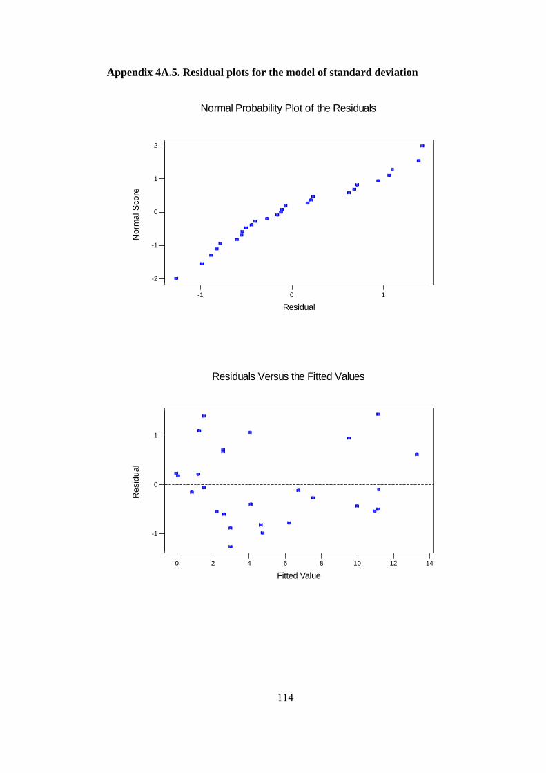
Appendix 4A.5. Residual plots for the model of standard deviation
114
10-1
2
1
0
-1
-2
Nor
mal
Sco
re
Residual
Normal Probability Plot of the Residuals
14121086420
1
0
-1
Fitted Value
Res
idua
l
Residuals Versus the Fitted Values
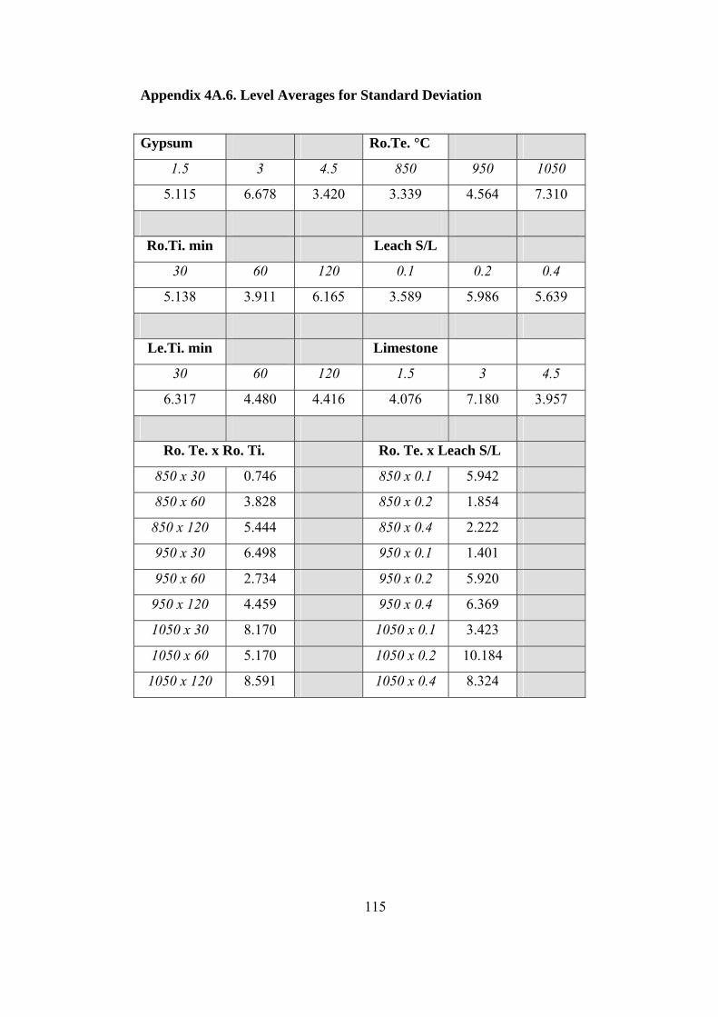
Appendix 4A.6. Level Averages for Standard Deviation Gypsum Ro.Te. °C
1.5 3 4.5 850 950 1050
5.115 6.678 3.420 3.339 4.564 7.310
Ro.Ti. min Leach S/L
30 60 120 0.1 0.2 0.4
5.138 3.911 6.165 3.589 5.986 5.639
Le.Ti. min Limestone
30 60 120 1.5 3 4.5
6.317 4.480 4.416 4.076 7.180 3.957
Ro. Te. x Ro. Ti. Ro. Te. x Leach S/L
850 x 30 0.746 850 x 0.1 5.942
850 x 60 3.828 850 x 0.2 1.854
850 x 120 5.444 850 x 0.4 2.222
950 x 30 6.498 950 x 0.1 1.401
950 x 60 2.734 950 x 0.2 5.920
950 x 120 4.459 950 x 0.4 6.369
1050 x 30 8.170 1050 x 0.1 3.423
1050 x 60 5.170 1050 x 0.2 10.184
1050 x 120 8.591 1050 x 0.4 8.324
115

Computation of the predicted standard deviation based on the optimum points of S/N Analysis:
From the level averages table; E(σ) = 5.071 + (3.420-5.071) + (4.564–5.071) + (6.165-5.071) + (5.986-5.071)
+ (4.416-5.071) + (4.076-5.071) + (3.872-5.071) + (5.512-5.071)
E(σ) = 5.071 – 1.651 – 0.507 + 1.094 + 0.915 – 0.655 - 0.995 - 1.199 + 0.441 = 2.514
116
)(
)()()()()()()()(
22
32132323
TxDB
TxCBTFTETDTCTBTATE
−+
−+−+−+−+−+−+−+=σ

Appendix 4A.7. The regression model with only main factors The regression equation is Mean = - 87.0 + 1.52*A + 0.110*B + 0.166*C - 2.8*D + 0.103*E - 4.50*F Predictor Coef SE Coef T P Constant -86.95 39.30 -2.21 0.039 A 1.519 2.546 0.60 0.557 B 0.11044 0.03819 2.89 0.009 C 0.16603 0.08333 1.99 0.060 D -2.76 25.00 -0.11 0.913 E 0.10307 0.08333 1.24 0.230 F -4.499 2.546 -1.77 0.092 S = 16.20 R-Sq = 46.5% R-Sq(adj) = 30.4% Analysis of Variance Source DF SS MS F P Regression 6 4555.3 759.2 2.89 0.034 Residual Error 20 5249.3 262.5 Total 26 9804.6 Source DF Seq SS A 1 93.4
B 1 2195.5 C 1 1042.0 D 1 3.2 E 1 401.5 F 1 819.7 Unusual Observations Obs A Mean Fit SE Fit Residual St Resid 18 3.00 22.92 52.65 8.25 -29.73 -2.13R 25 4.50 13.68 44.14 8.50 -30.46 -2.21R R denotes an observation with a large standardized residual Durbin-Watson statistic = 2.44
117

Appendix 4A.8. The regression of the quadratic model A*E is highly correlated with other X variables A*E has been removed from the equation C*E is highly correlated with other X variables C*E has been removed from the equation D*E is highly correlated with other X variables D*E has been removed from the equation C*C is highly correlated with other X variables C*C has been removed from the equation D*D is highly correlated with other X variables D*D has been removed from the equation E*E is highly correlated with other X variables E*E has been removed from the equation The regression equation is
Mean = - 1332 + 17.2*A + 2.89*B - 0.105*C - 98.5*D + 0.631*E - 50.2*F + 0.0189*AB + 0.195*AC - 1.49*AD + 5.20*AF - 0.00121*BC -
0.142*BD -0.000631*BE + 0.0545*BF + 3.75*CD - 0.0134*CF - 2.97*DF - 9.80*A2 -0.00149*B2 - 3.49*F2
Predictor Coef SE Coef T P Contant -1332.1 129.5 -10.29 0.000 A 17.17 17.08 1.01 0.354 B 2.8857 0.2644 10.91 0.000 C -0.1051 0.3143 -0.33 0.749 D -98.52 95.90 -1.03 0.344 E 0.6312 0.4228 1.49 0.186 F -50.18 10.84 -4.63 0.004 A*B 0.018944 0.007003 2.71 0.035 A*C 0.19532 0.02154 9.07 0.000 A*D -1.491 6.461 -0.23 0.825 A*F 5.2019 0.4669 11.14 0.000 B*C -0.0012118 0.0002335 -5.19 0.002 B*D -0.14162 0.06711 -2.11 0.079 B*E -0.0006306 0.0003968 -1.59 0.163 B*F 0.05452 0.01212 4.50 0.004 C*D 3.7501 0.8618 4.35 0.005
118
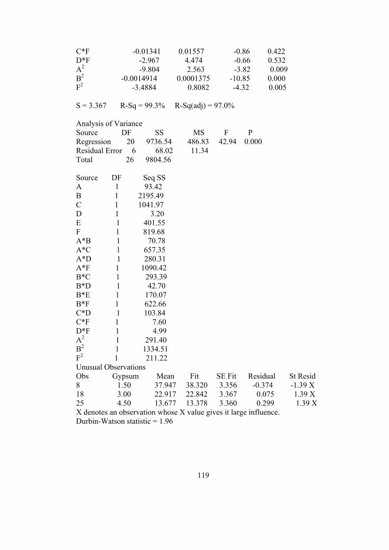
C*F -0.01341 0.01557 -0.86 0.422 D*F -2.967 4.474 -0.66 0.532 A2 -9.804 2.563 -3.82 0.009 B2 -0.0014914 0.0001375 -10.85 0.000 F2 -3.4884 0.8082 -4.32 0.005 S = 3.367 R-Sq = 99.3% R-Sq(adj) = 97.0% Analysis of Variance Source DF SS MS F P Regression 20 9736.54 486.83 42.94 0.000 Residual Error 6 68.02 11.34 Total 26 9804.56 Source DF Seq SS A 1 93.42 B 1 2195.49 C 1 1041.97 D 1 3.20 E 1 401.55 F 1 819.68 A*B 1 70.78 A*C 1 657.35 A*D 1 280.31 A*F 1 1090.42 B*C 1 293.39 B*D 1 42.70 B*E 1 170.07 B*F 1 622.66 C*D 1 103.84 C*F 1 7.60 D*F 1 4.99 A2 1 291.40 B2 1 1334.51 F2 1 211.22 Unusual Observations Obs Gypsum Mean Fit SE Fit Residual St Resid 8 1.50 37.947 38.320 3.356 -0.374 -1.39 X 18 3.00 22.917 22.842 3.367 0.075 1.39 X 25 4.50 13.677 13.378 3.360 0.299 1.39 X X denotes an observation whose X value gives it large influence. Durbin-Watson statistic = 1.96
119

Appendix 4A.9. Regression Analysis for Improved Quadratic Model: The regression equation is Mean = -1332 +18.2*A +2.89*B -0.121*C -108*D +0.629*E -50.2*F
+0.0189*AB+0.195*AC +5.20*AF - 0.00121*BC-0.142*BD-0.000631*BE + 0.0545*BF+ 3.82*CD-0.0134*CF-2.97*DF-10.0*A2- 0.00149*B2- 3.49*F2
Predictor Coef SE Coef T P Constant -1331.6 120.4 -11.06 0.000 A 18.19 15.34 1.19 0.275 B 2.8857 0.2459 11.73 0.000 C -0.1209 0.2853 -0.42 0.684 D -108.21 80.18 -1.35 0.219 E 0.6288 0.3930 1.60 0.154 F -50.18 10.08 -4.98 0.002 A*B 0.018944 0.006512 2.91 0.023 A*C 0.19532 0.02003 9.75 0.000 A*F 5.2019 0.4341 11.98 0.000 B*C -0.0012118 0.0002172 -5.58 0.001 B*D -0.14162 0.06241 -2.27 0.058 B*E -0.0006306 0.0003690 -1.71 0.131 B*F 0.05452 0.01127 4.84 0.002 C*D 3.8247 0.7430 5.15 0.001 C*F -0.01341 0.01448 -0.93 0.385 D*F -2.967 4.160 -0.71 0.499 A2 -10.020 2.220 -4.51 0.003 B2 -0.0014914 0.0001278 -11.67 0.000 F2 -3.4884 0.7515 -4.64 0.002 S = 3.131 R-Sq = 99.3% R-Sq(adj) = 97.4% Analysis of Variance Source DF SS MS F P Regression 19 9735.94 512.42 52.27 0.000 Residual Error 7 68.62 9.80 Total 26 9804.56
120

Source DF Seq SS A 1 93.42 B 1 2195.49 C 1 1041.97 D 1 3.20 E 1 401.55 F 1 819.68 A*B 1 70.78 A*C 1 657.35 A*F 1 1090.42 B*C 1 293.39 B*D 1 42.70 B*E 1 170.07 B*F 1 824.40 C*D 1 122.09 C*F 1 7.60 D*F 1 4.99 A2 1 351.11 B2 1 1334.51 F2 1 211.22 Unusual Observations Obs Jips Ort. Fit SE Fit Residual St Resid 18 3.00 22.917 22.773 3.118 0.144 0.51 X X denotes an observation whose X value gives it large influence.
Durbin-Watson statistic = 1.99
121
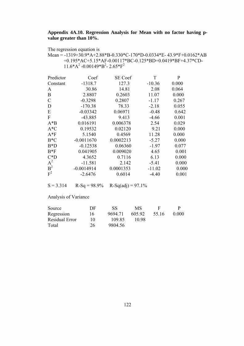
Appendix 4A.10. Regression Analysis for Mean with no factor having p-value greater than 10%. The regression equation is Mean = -1319+30.9*A+2.88*B-0.330*C-170*D-0.0334*E- 43.9*F+0.0162*AB
+0.195*AC+5.15*AF-0.00117*BC-0.125*BD+0.0419*BF+4.37*CD- 11.6*A2 -0.00149*B2- 2.65*F2
Predictor Coef SE Coef T P Constant -1318.7 127.3 -10.36 0.000 A 30.86 14.81 2.08 0.064 B 2.8807 0.2603 11.07 0.000 C -0.3298 0.2807 -1.17 0.267 D -170.38 78.33 -2.18 0.055 E -0.03342 0.06971 -0.48 0.642 F -43.885 9.413 -4.66 0.001 A*B 0.016191 0.006378 2.54 0.029 A*C 0.19532 0.02120 9.21 0.000 A*F 5.1540 0.4569 11.28 0.000 B*C -0.0011670 0.0002213 -5.27 0.000 B*D -0.12538 0.06360 -1.97 0.077 B*F 0.041905 0.009020 4.65 0.001 C*D 4.3652 0.7116 6.13 0.000 A2 -11.581 2.142 -5.41 0.000 B2 -0.0014914 0.0001353 -11.02 0.000 F2 -2.6476 0.6014 -4.40 0.001 S = 3.314 R-Sq = 98.9% R-Sq(adj) = 97.1% Analysis of Variance Source DF SS MS F P Regression 16 9694.71 605.92 55.16 0.000 Residual Error 10 109.85 10.98 Total 26 9804.56
122

Source DF Seq SS A 1 93.42 B 1 2195.49 C 1 1041.97 D 1 3.20 E 1 401.55 F 1 819.68 A*B 1 70.78 A*C 1 657.35 A*F 1 1090.42 B*C 1 293.39 B*D 1 42.70 B*F 1 991.83 C*D 1 124.40 A2 1 321.12 B2 1 1334.51 F2 1 212.92 Durbin-Watson statistic = 1.38
123

Appendix 4A.11. The Best Regression Model for s. The regression equation is s = - 1.53 - 79.6*D + 6.42*F + 0.0380*AC - 6.64*AD + 0.659*AF-
0.000113*BC + 0.115*BD - 0.619*A2 - 1.41*F2 C6C6 Predictor Coef SE Coef T P Constant -1.525 5.034 -0.30 0.766 D -79.61 27.37 -2.91 0.010 F 6.420 3.366 1.91 0.074 A*C 0.03805 0.01361 2.80 0.012 A*D -6.639 4.249 -1.56 0.137 A*F 0.6591 0.3541 1.86 0.080 B*C -0.00011261 0.00004762 -2.36 0.030 B*D 0.11453 0.02821 4.06 0.001 A2 -0.6188 0.2371 -2.61 0.018 F2 -1.4062 0.5268 -2.67 0.016 S = 2.904 R-Sq = 67.7% R-Sq(adj) = 50.6% Analysis of Variance Source DF SS MS F P Regression 9 300.633 33.404 3.96 0.007 Residual Error 17 143.330 8.431 Total 26 443.963 Source DF Seq SS D 1 13.215 F 1 0.063 A*C 1 2.783 A*D 1 32.281 A*F 1 4.337 B*C 1 0.497 B*D 1 129.973 A2 1 57.423 F2 1 60.060 Unusual Observations Obs D s Fit SE Fit Residual St Resid
2 0.200 0 .664 7.051 1.518 -6.386 -2.58R R denotes an observation with a large standardized residual Durbin-Watson statistic = 2.70
124

Appendix 4A.12. The Values of Log s2:
Run No s log s2 1 6.6044 1.6397 2 0.6643 -0.3553 3 1.9970 0.6008 4 1.6983 0.4600 5 5.4060 1.4658 6 3.8339 1.1673 7 2.8498 0.9096 8 10.4453 2.0378 9 12.5324 2.1961 10 1.6251 0.4218 11 1.4144 0.3011 12 11.0631 2.0878 13 5.1102 1.4169 14 13.8822 2.2849 15 2.2984 0.7228 16 10.5982 2.0505 17 10.3786 2.0323 18 3.7331 1.1441 19 3.2547 1.0250 20 0.1582 -1.60148 21 3.2723 1.0297 22 1.3922 0.2874 23 0.2066 -1.3696 24 7.2443 1.7200 25 2.0619 0.6285 26 3.6848 1.1328 27 9.5077 1.9562
125

Appendix 4A.13. The regression model for log s2
* A*E is highly correlated with other X variables * A*E has been removed from the equation * C*E is highly correlated with other X variables * C*E has been removed from the equation * D*E is highly correlated with other X variables * D*E has been removed from the equation * C2 is highly correlated with other X variables * C2 has been removed from the equation * D2 is highly correlated with other X variables * D2 has been removed from the equation * E2 is highly correlated with other X variables * E2 has been removed from the equation The regression equation is Log s2 = 9.1 + 1.81*A - 0.0249*B + 0.0583*C - 8.2*D - 0.058*E + 0.17*F -
0.00003*AB + 0.00824*AC + 0.35*AD + 0.145*AF -0.000099*BC + 0.0026*BD +0.000054*BE + 0.00051*BF + 0.087*CD - 0.00035*CF + 0.33*DF - 0.499 A2 +0.000016*B2- 0.185*F2
Predictor Coef SE Coef T P Constant 9.10 34.96 0.26 0.803 A 1.815 4.611 0.39 0.708 B -0.02486 0.07139 -0.35 0.740 C 0.05833 0.08486 0.69 0.518 D -8.19 25.89 -0.32 0.762 E -0.0577 0.1141 -0.51 0.631 F 0.167 2.925 0.06 0.956 A*B -0.000025 0.001891 -0.01 0.990 A*C 0.008236 0.005814 1.42 0.206 A*D 0.348 1.744 0.20 0.848 A*F 0.1453 0.1260 1.15 0.293 B*C -0.00009883 0.00006305 -1.57 0.168 B*D 0.00260 0.01812 0.14 0.891 B*E 0.0000543 0.0001071 0.51 0.630 B*F 0.000507 0.003273 0.15 0.882 C*D 0.0873 0.2327 0.38 0.720
126

C*F -0.000353 0.004203 -0.08 0.936 D*F 0.325 1.208 0.27 0.797 A2 -0.4990 0.6921 -0.72 0.498 B2 0.00001626 0.00003711 0.44 0.677 F2 -0.1847 0.2182 -0.85 0.430 S = 0.9090 R-Sq = 81.0% R-Sq(adj) = 17.5% Analysis of Variance Source DF SS MS F P Regression 20 21.0721 1.0536 1.28 0.408 Residual Error 6 4.9576 0.8263 Total 26 26.0297 Source DF Seq SS A 1 1.5683 B 1 4.4391 C 1 2.4724 D 1 1.0978 E 1 2.1192 F 1 0.0801 A*B 1 0.0000 A*C 1 1.4998 A*D 1 0.0062 A*F 1 0.4114 B*C 1 2.4293 B*D 1 0.0234 B*E 1 1.9276 B*F 1 0.0165 C*D 1 1.3937 C*F 1 0.0086 D*F 1 0.0599 A2 1 0.7683 B2 1 0.1585 F2 1 0.5919 Unusual Observations Obs Gypsum Log s2 Fit SE Fit Residual St Resid
8 1.50 2.038 2.027 0.906 0.011 0.15 X 18 3.00 1.144 1.146 0.909 -0.002 -0.15 X 25 4.50 0.629 0.637 0.907 -0.009 -0.15 X X denotes an observation whose X value gives it large influence. Durbin-Watson statistic = 2.12
127

Appendix 4A.14. Regression Analysis for improved quadratic model of log s2 The regression equation is Log s2 = - 4.00 + 0.0905*C + 0.00632*AC + 0.670*AD + 0.158*AF -
0.000106*BC + 0.00117*BF - 0.212 A2 +0.000005*B2 -0.271*F2 Predictor Coef SE Coef T P Constant -4.005 1.499 -2.67 0.016 C 0.09051 0.03739 2.42 0.027 A*C 0.006320 0.002397 2.64 0.017 A*D 0.6700 0.2775 2.41 0.027 A*F 0.15803 0.07296 2.17 0.045 B*C -0.00010596 0.00003840 -2.76 0.013 B*F 0.0011689 0.0006075 1.92 0.071 A2 -0.21231 0.04785 -4.44 0.000 B2 0.00000468 0.00000191 2.45 0.025 F2 -0.27120 0.09254 -2.93 0.009 S = 0.5817 R-Sq = 77.9% R-Sq(adj) = 66.2% Analysis of Variance Source DF SS MS F P Regression 9 20.2778 2.2531 6.66 0.000 Residual Error 17 5.7519 0.3383 Total 26 26.0297 Source DF Seq SS C 1 2.4724 A*C 1 0.1371 A*D 1 0.3631 A*F 1 0.8135 B*C 1 1.7253 B*F 1 2.3838 A2 1 3.7372 B2 1 5.7395 F2 1 2.9059 Unusual Observations Obs Ro.Ti. Log s2 Fit SEFit Residual St Resid 2 30 -0.355 0.650 0.336 -1.006 -2.12R 5 30 1.466 0.496 0.357 0.970 2.11R R denotes an observation with a large standardized residual Durbin-Watson statistic = 2.43
128

Appendix 4A.15. Regression Analysis for log s2 with cubic terms The regression equation is Log s2 = - 2.58 + 0.0592*C + 0.00858*AC -0.000081*BC +0.000873*BF -
0.0273*A3 +0.000000*B3 + 10.6*D3 - 0.0298*F3 Predictor Coef SE Coef T P Constant -2.579 1.094 -2.36 0.030 C 0.05921 0.03772 1.57 0.134 A*C 0.008584 0.002529 3.39 0.003 B*C -0.00008092 0.00003874 -2.09 0.051 B*F 0.0008730 0.0003786 2.31 0.033 A3 -0.027280 0.006500 -4.20 0.001 B3 0.00000000 0.00000000 2.46 0.024 D3 10.609 4.543 2.34 0.031 F3 -0.02979 0.01192 -2.50 0.022 S = 0.6189 R-Sq = 73.5% R-Sq(adj) = 61.7% Analysis of Variance Source DF SS MS F P Regression 8 19.1354 2.3919 6.24 0.001 Residual Error 18 6.8943 0.3830 Total 26 26.0297 Source DF Seq SS C 1 2.4724 A*C 1 0.1371 B*C 1 1.5948 B*F 1 0.0021 A3 1 5.6569 B3 1 4.6278 D3 1 2.2535 F3 1 2.3907 Unusual Observations Obs Ro.Ti. Log s2 Fit SE Fit Residual St Resid 1 60 1.640 0.367 0.283 1.273 2.31R 2 30 -0.355 0.751 0.342 -1.107 -2.15R R denotes an observation with a large standardized residual Durbin-Watson statistic = 2.09
129

APPENDIX 5A
130


Appendix 5A.1. The Starting and Optimum Points for Minitab Response Optimizer
STARTING POINTS OPTIMUM POINTS
POINTS Gypsum
Ratio
Roast.
Temp.
(°C)
Roasting
Time
(min)
Leach
S/L
Ratio
Leach
Time
(min)
Limestone
Ratio
Gypsum
Ratio
Roast.
Temp.
(°C)
Roasting
Time
(min)
Leach
S/L
Ratio
Leach
Time
(min)
Limestone
Ratio
1 1.5 987 30 0.1 120 1.5 1.5 987 30 0.1 120 1.5
2 3.23 900 120 0.4 40 2.32 3.23 900 120 0.4 40 2.32
3 4.5 900 30 0.1 120 1.5 4.5 900 30 0.1 120 1.5
4 1.5 878 120 0.36 120 1.5 1.5 878 120 0.36 120 1.5
5 3 950 60 0.2 60 3 3 950 60 0.2 60 3
6 2 1000 100 0.4 60 2 2 1000 100 0.4 60 2
7 NO STARTING POINT 4.5 850 120 0.4 120 1.5
8 3 970 30 0.2 120 3 3 970 30 0.112 120 2.41
9 4.5 900 120 0.4 30 1.5 4.5 900 120 0.4 30 1.5
10 4.5 950 60 0.3 30 4.5 4.5 950 60 0.3 30 4.5
131

Appendix 5A.2. GAMS Input Program variable S, Z; positive variable A, B, C, D, E, F; EQUATIONS OB, EQ, EQ100, EQS, A1, A2,B1, B2 , C1,C2,D1,D2,E1,E2,F1,F2; OB.. Z=e= -1331.6 + 18.19*A+ 2.8857*B - 0.1209*C - 108.21*D + 0.6288*E - 50.18*F + 0.018944*A*B + 0.19532*A*C + 5.2019*A*F - 0.0012118*B*C - 0.14162*B*D -0.0006306*B*E + 0.05452*B*F + 3.8247*C*D - 0.01341*C*F - 2.967*D*F - 10.02*A*A-0.0014914*B*B - 3.4884*F*F;
EQ.. -2.579 + 0.05921*C + 0.008584*A*C - 0.00008092*B*C + 0.000873*B*F -0.02728*A*A*A+0.0000000015*B*B*B+10.609*D*D*D-0.02979*F*F*F =l=1;
EQ100.. -1331.6 + 18.19*A+ 2.8857*B - 0.1209*C - 108.21*D + 0.6288*E - 50.18*F +0.018944*A*B + 0.19532*A*C + 5.2019*A*F - 0.0012118*B*C - 0.14162*B*D -0.0006306*B*E + 0.05452*B*F + 3.8247*C*D - 0.01341*C*F - 2.967*D*F - 10.02*A*A-0.0014914*B*B - 3.4884*F*F=l=100 ;
EQS..-2.579 + 0.05921*C + 0.008584*A*C - 0.00008092*B*C + 0.000873*B*F -0.02728*A*A*A + 0.0000000015*B*B*B + 10.609*D*D*D - 0.02979*F*F*F =e=S;
A1.. A=l=4.5; A2.. A=g=1.5; B1.. B=l=1050; B2.. B=g=850; C1.. C=l=120; C2.. C=g=30; D1.. D=l=0.4; D2.. D=g=0.1; E1.. E=l=120; E2.. E=g=30; F1.. F=l=4.5; F2.. F=g=1.5; MODEL ATIL1 /ALL/ ; SOLVE ATIL1 USING NLP MAXIMIZING Z;
132
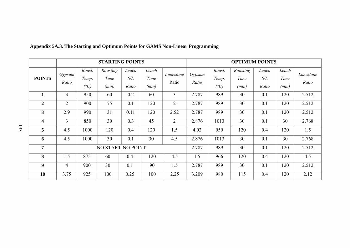
Appendix 5A.3. The Starting and Optimum Points for GAMS Non-Linear Programming
STARTING POINTS OPTIMUM POINTS
POINTS Gypsum
Ratio
Roast.
Temp.
(°C)
Roasting
Time
(min)
Leach
S/L
Ratio
Leach
Time
(min)
Limestone
Ratio
Gypsum
Ratio
Roast.
Temp.
(°C)
Roasting
Time
(min)
Leach
S/L
Ratio
Leach
Time
(min)
Limestone
Ratio
1 3 950 60 0.2 60 3 2.787 989 30 0.1 120 2.512
2 2 900 75 0.1 120 2 2.787 989 30 0.1 120 2.512
3 2.9 990 31 0.11 120 2.52 2.787 989 30 0.1 120 2.512
4 3 850 30 0.3 45 2 2.876 1013 30 0.1 30 2.768
5 4.5 1000 120 0.4 120 1.5 4.02 959 120 0.4 120 1.5
6 4.5 1000 30 0.1 30 4.5 2.876 1013 30 0.1 30 2.768
7 NO STARTING POINT 2.787 989 30 0.1 120 2.512
8 1.5 875 60 0.4 120 4.5 1.5 966 120 0.4 120 4.5
9 4 900 30 0.1 90 1.5 2.787 989 30 0.1 120 2.512
10 3.75 925 100 0.25 100 2.25 3.209 980 115 0.4 120 2.12
133

C1 C2 C3 C4 C5 C6 C1 -10.02 0.0095 0.098 0 0 2.6 B= C2 0.0095 -0.0015 -0.0006 -0.071 -0.00032 0.027
C3 0.098 -0.0006 0 1.912 0 -0.0067
C4 -0.75 -0.071 1.912 0 0 -1.484 C5 0 -0.00032 0 0 0 0 C6 2.6 0.027 -0.0067 -1.484 0 -3.49
C1 C2 C3 C4 C5 C6 C1 -10.02-L 0.0095 0.098 -0.75 0 2.6 X1 18.19
B-LI= C2 0.0095 -0.0015-L -0.0006 -0.071 -0.00032 0.027 X2 2.886
C3 0.098 -0.0006 -L 1.912 0 -0.0067 X3 -0.5 = -0.1209
C4 -0.75 -0.071 1.912 -L 0 -1.484 X4 -108.21
C5 0 -0.00032 0 0 -L 0 X5 0.6288 C6 2.6 0.027 -0.0067 -1.484 0 -3.49-L X6 -50.18
EIGENVALUES
-10.9511 -3.4231 -1.2753 -0.0013 0.0001 2.1392
134

Appendix 5A.5. Solving of Ridge Analysis for λ Inside the Region of the Experiments Variable G,Z; positive variable A, B, C, D, E, F, L; EQUATIONS OB, P, Q, R, S, T, U, V, Y, X; OB.. Z=e=1; P.. (-10.02-L)*A+0.0095*B+0.098*C+2.6*F=e=-9.095; Q.. 0.0095*A-(0.0015+L)*B-0.0006*C-0.071*D-0.00032*E+0.027*F=e=-
1.443; R.. 0.098*A-0.0006*B-L*C+1.912*D-0.0067*F=e=0.06045; S.. -0.071*B+1.912*C-L*D-1.484*F=e=54.105; T.. -0.00032*B-L*E=e=-0.3144; U.. 2.6*A+0.027*B-0.0067*C-1.484*D-(3.49+L)*F=e=25.09; V.. L=l=2.1392; Y.. L=g=-10.9511; X.. G=e=L; MODEL ATIL2 /ALL/ ; SOLVE ATIL2 USING NLP MAXIMIZING Z ;
SOLUTION PROPOSED BY GAMS LOWER LEVEL UPPER MARGINAL VAR G -INF . +INF . VAR Z -INF 1.000 +INF . VAR A . 3.155 +INF . VAR B . 982.500 +INF . VAR C . 66.764 +INF . VAR D . 0.187 +INF . VAR E . 46.404 +INF . VAR F . 2.555 +INF . VAR L . . +INF EPS **** λ=0 is the solution for the case that –10.391<λ<2.1392
135

Appendix 5A.6. Solving of Ridge Analysis for λ Outside the Region of the Experiments Variable G,Z; positive variable A, B, C, D, E, F, L; EQUATIONS OB, P, Q, R, S, T, U, V, Y, X; OB.. Z=e=1; P.. (-10.02-L)*A+0.0095*B+0.098*C+2.6*F=e=-9.095; Q.. 0.0095*A-(0.0015+L)*B-0.0006*C-0.071*D-0.00032*E+0.027*F=e=-
1.443; R.. 0.098*A-0.0006*B-L*C+1.912*D-0.0067*F=e=0.06045; S.. -0.071*B+1.912*C-L*D-1.484*F=e=54.105; T.. -0.00032*B-L*E=e=-0.3144; U.. 2.6*A+0.027*B-0.0067*C-1.484*D-(3.49+L)*F=e=25.09; V.. L=g=2.1392; Y.. L=l=-10.9511; X.. G=e=L; MODEL ATIL2 /ALL/ ; SOLVE ATIL2 USING NLP MAXIMIZING Z ;
SOLUTION PROPOSED BY GAMS SOLVER STATUS 1 NORMAL COMPLETION **** MODEL STATUS 5 LOCALLY INFEASIBLE **** OBJECTIVE VALUE 1.0000 ** Infeasible solution. There are no superbasic variables.
LOWER LEVEL UPPER MARGINAL VAR G -INF . +INF . VAR Z -INF 1.000 +INF . VAR A . 3.155 +INF . VAR B . 982.500 +INF . VAR C . 66.764 +INF . VAR D . 0.187 +INF . VAR E . 46.404 +INF . VAR F . 2.555 +INF . VAR L . . +INF EPS
136

APPENDIX 6A
137

Appendix 6A.1. The Starting Model for Mean Including Optimum Points
The regression equation is Ort. = 1013+67.4*A-2.55*B-0.61*C+708*D-10.0*E+312*F +0.0189*AB-0.313*AC+112*AD+0.261*AE+5.20*AF -0.00121*BC-0.142*BD+0.00944*B-0.348*BF+12.3*CD+0.00611*CE-
0.0134*CF-8.39*DE-2.97*DF-0.671*EF- 20.7*A2+0.00153*B2+0.00418*C22322*D2+0.0158*E2+9.94*F2
Predictor Coef SE Coef T P Constant 1013.0 507.9 1.99 0.093 A 67.39 24.49 2.75 0.033 B -2.552 1.309 -1.95 0.099 C -0.608 1.431 -0.42 0.686 D 707.8 619.2 1.14 0.297 E -10.047 1.806 -5.56 0.001 F 312.31 82.40 3.79 0.009 A*B 0.018944 0.007003 2.71 0.035 A*C -0.3132 0.1153 -2.72 0.035 A*D 111.57 36.70 3.04 0.023 A*E 0.2606 0.4480 0.58 0.582 A*F 5.2019 0.4669 11.14 0.000 B*C -0.0012118 0.0002335 -5.19 0.002 B*D -0.14162 0.06711 -2.11 0.079 B*E 0.009438 0.002241 4.21 0.006 B*F -0.34824 0.09107 -3.82 0.009 C*D 12.322 5.422 2.27 0.063 C*E 0.006107 0.009801 0.62 0.556 C*F -0.01341 0.01557 -0.86 0.422 D*E -8.391 7.310 -1.15 0.295 D*F -2.967 4.474 -0.66 0.532 E*F -0.6713 0.1587 -4.23 0.006 A2 -20.699 5.789 -3.58 0.012 B2 0.0015293 0.0007258 2.11 0.080 C2 0.004180 0.004917 0.85 0.428 D2 -2322.4 797.9 -2.91 0.027 E2 0.015767 0.003582 4.40 0.005 F2 9.937 3.123 3.18 0.019 S = 3.367 R-Sq = 99.6% R-Sq(adj) = 97.7%
138

Analysis of Variance Source DF SS MS F P Regression 27 16260.81 602.25 53.12 0.000 Residual Error 6 68.02 11.34 Total 33 16328.83 Source DF Seq SS A 1 11.65 B 1 2464.23 C 1 1646.34 D 1 334.88 E 1 1238.54 F 1 1849.67 A*B 1 161.83 A*C 1 171.29 A*D 1 154.45 A*E 1 1295.18 A*F 1 976.63 B*C 1 263.47 B*D 1 17.57 B*E 1 25.98 B*F 1 463.35 C*D 1 21.84 C*E 1 2083.92 C*F 1 4.96 D*E 1 698.48 D*F 1 6.09 E*F 1 520.25 A2 1 785.81 B2 1 443.22 C2 1 208.88 D2 1 114.72 E2 1 182.79 F2 1 114.77 Unusual Observations Obs Gyp Ort. Fit SE Fit Residual St Resid 8 1.50 37.947 38.320 3.356 -0.374 -1.39 X 18 3.00 22.917 22.842 3.367 0.075 1.39 X 25 4.50 13.677 13.378 3.360 0.299 1.39 X 28 1.50 62.355 62.355 3.367 -0.000 * X 29 1.50 72.110 72.110 3.367 -0.000 * X
139

30 1.50 43.105 43.105 3.367 -0.000 * X 31 3.18 75.200 75.200 3.367 -0.000 * X 32 2.77 52.530 52.530 3.367 -0.000 * X 33 4.50 62.330 62.330 3.367 -0.000 * X 34 4.50 22.695 22.695 3.367 -0.000 * X X denotes an observation whose X value gives it large influence. Durbin-Watson statistic = 1.98
140
80706050403020100
3
2
1
0
-1
-2
-3
F itted Value
Res
idua
l
3210-1-2-3
2
1
0
-1
-2
Nor
mal
Sco
re
Residual

Appendix 6A.2. The Regression Model Comprising Optimum Points With No Factor Having P-Value Greater Than 10% Regression Analysis: Mean versus Gypsum; Ro.Te.; ... The regression equation is Mean = 703 + 77.4*A - 1.70*B - 1.36*C + 337*D- 9.14*E + 255*F + 0.0163*AB-0.248*AC + 90.6*AD+ 5.10*AF - 0.00115*BC - 0.121*BD + 0.00792*BE -0.287*BF + 8.95*CD + 0.0116*CE - 4.09*DE - 0.567*EF - 17.0*A2 + 0.00106*B2 + 0.00582*C2 – 1842*D2 + 0.0157*E2 + 7.87*F2 Predictor Coef SE Coef T P Constant 702.9 319.7 2.20 0.055 A 77.44 13.32 5.82 0.000 B -1.7035 0.6852 -2.49 0.035 C -1.3554 0.4839 -2.80 0.021 D 337.09 71.11 4.74 0.001 E -9.141 1.443 -6.34 0.000 F 255.44 40.00 6.39 0.000 A*B 0.016252 0.005850 2.78 0.021 A*C -0.24790 0.05860 -4.23 0.002 A*D 90.57 20.01 4.53 0.001 A*F 5.1048 0.4086 12.49 0.000 B*C -0.0011496 0.0002003 -5.74 0.000 B*D -0.12117 0.05779 -2.10 0.065 B*E 0.007921 0.001108 7.15 0.000 B*F -0.28658 0.04403 -6.51 0.000 C*D 8.9461 0.8377 10.68 0.000 C*E 0.011551 0.001304 8.86 0.000 D*E -4.0862 0.7136 -5.73 0.000 E*F -0.56656 0.07959 -7.12 0.000 A2 -16.963 2.004 -8.47 0.000 B2 0.0010576 0.0003752 2.82 0.020 C2 0.005822 0.003073 1.89 0.091 D2 -1842.2 221.1 -8.33 0.000 E2 0.015701 0.002881 5.45 0.000 F2 7.874 1.592 4.94 0.001
S = 3.040 R-Sq = 99.5% R-Sq(adj) = 98.1% Analysis of Variance Source DF SS MS F P Regression 24 16245.64 676.90 73.23 0.000 Residual Error 9 83.19 9.24 Total 33 16328.83 Durbin-Watson statistic = 1.64
141

Appendix 6A.3. The Best Regression Model Comprising Optimum Points
Regression Analysis: Mean versus Gypsum; Ro.Te; ..
The regression equation is Mean = 769 + 78.2*A - 1.85*B - 1.38*C + 343*D - 9.46*E + 266*F + 0.0181*AB - 0.254*AC + 93.2*AD + 5.12*AF - 0.00115*BC
- 0.135*BD + 0.00819*BE - 0.297*BF + 9.09*CD + 0.0116*CE - 0.0124*CF - 4.09*DE - 0.584*EF - 17.4*A2 + 0.00114*B2 + + 0.00614*C2 – 1864*D2 + 0.0162*E2 + 8.23*F2
Predictor Coef SE Coef T P Constant 768.8 332.8 2.31 0.050 A 78.16 13.52 5.78 0.000 B -1.8507 0.7148 -2.59 0.032 C -1.3787 0.4912 -2.81 0.023 D 342.71 72.37 4.74 0.001 E -9.458 1.507 -6.28 0.000 F 266.01 42.32 6.29 0.000 A*B 0.018113 0.006303 2.87 0.021 A*C -0.25436 0.05986 -4.25 0.003 A*D 93.18 20.50 4.55 0.002 A*F 5.1191 0.4145 12.35 0.000 B*C -0.0011513 0.0002031 -5.67 0.000 B*D -0.13523 0.06076 -2.23 0.057 B*E 0.008193 0.001166 7.03 0.000 B*F -0.29740 0.04633 -6.42 0.000 C*D 9.0914 0.8654 10.51 0.000 C*E 0.011571 0.001322 8.75 0.000 C*F -0.01238 0.01421 -0.87 0.409 D*E -4.0865 0.7233 -5.65 0.000 E*F -0.58447 0.08325 -7.02 0.000 A2 -17.383 2.087 -8.33 0.000 B2 0.0011381 0.0003914 2.91 0.020 C2 0.006138 0.003136 1.96 0.086 D2 -1863.7 225.5 -8.27 0.000 E2 0.016246 0.002986 5.44 0.001 F2 8.235 1.666 4.94 0.001 S = 3.082 R-Sq = 99.5% R-Sq(adj) = 98.1%
142

Analysis of Variance Source DF SS MS F P Regression 25 16252.85 650.11 68.46 0.000 Residual Error 8 75.97 9.50 Total 33 16328.83 Source DF Seq SS A 1 11.65 B 1 2464.23 C 1 1646.34 D 1 334.88 E 1 1238.54 F 1 1849.67 A*B 1 161.83 A*C 1 171.29 A*D 1 154.45 A*F 1 1815.20 B*C 1 314.76 B*D 1 15.69 B*E 1 80.25 B*F 1 271.47 C*D 1 7.86 C*E 1 50.33 C*F 1 0.22 D*E 1 580.79 E*F 1 600.13 A2 1 1077.26 B2 1 1052.49 C2 1 1580.49 D2 1 482.01 E2 1 59.07 F2 1 231.95 Unusual Observations Obs Gypsum Mean Fit SE Fit Residual St Resid 33 4.50 62.330 62.171 3.069 0.159 0.56 X X denotes an observation whose X value gives it large influence.
Durbin-Watson statistic = 1.96
143


Appendix 6A.4. The Starting and Optimum Points for Minitab Response Optimizer for maximizing extraction while minimizing variation
STARTING POINTS OPTIMUM POINTS
POINTS Gypsum
Ratio
Roast.
Temp.
(°C)
Roasting
Time
(min)
Leach
S/L
Ratio
Leach
Time
(min)
Limestone
Ratio
Gypsum
Ratio
Roast.
Temp.
(°C)
Roasting
Time
(min)
Leach
S/L
Ratio
Leach
Time
(min)
Limestone
Ratio
1 1.5 918 120 0.17 120 1.5 1.5 918 120 0.17 120 1.5
2 1.5 940 120 0.15 120 1.5 1.53 940 120 0.15 120 1.5
3 1.5 950 120 0.17 120 2 1.57 950 120 0.15 120 1.77
4 1.5 915 120 0.26 120 1.5 1.5 915 120 0.26 120 1.5
5 1.5 915 120 0.25 120 2 1.5 915 120 0.25 120 2
6 1.5 940 120 0.2 120 1.5 1.5 940 120 0.2 120 1.5
7 NO STARTING POINT 4.5 850 120 0.1 30 4.5
8 1.5 1000 60 0.4 45 1.5 4.39 1000 59 0.31 41 4.5
9 1.5 1050 30 0.1 120 1.5 1.5 1050 30 0.1 120 1.5
10 3.178 986 67 0.187 33 2.6 3.178 986 67 0.18 30 3.03
144
