robust creation of implicit surfaces from polygon meshes
TRANSCRIPT
Robust Creation of Implicit Surfaces from Polygon
MeshesGary Yngve and Greg Turk
Presented by Owen Gray
Overview● Implicit Surface Generation● Volumetric Representation of Objects● Implicit Surfaces● Evaluation of surface fit● Choice of constraints● Eye candy
Implicit Surface Generation
2
∫∑i , j
2 f x xi x j
d x
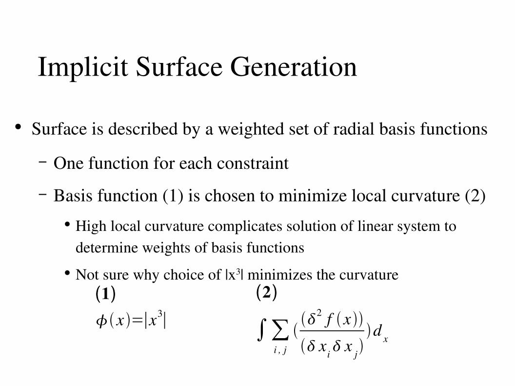
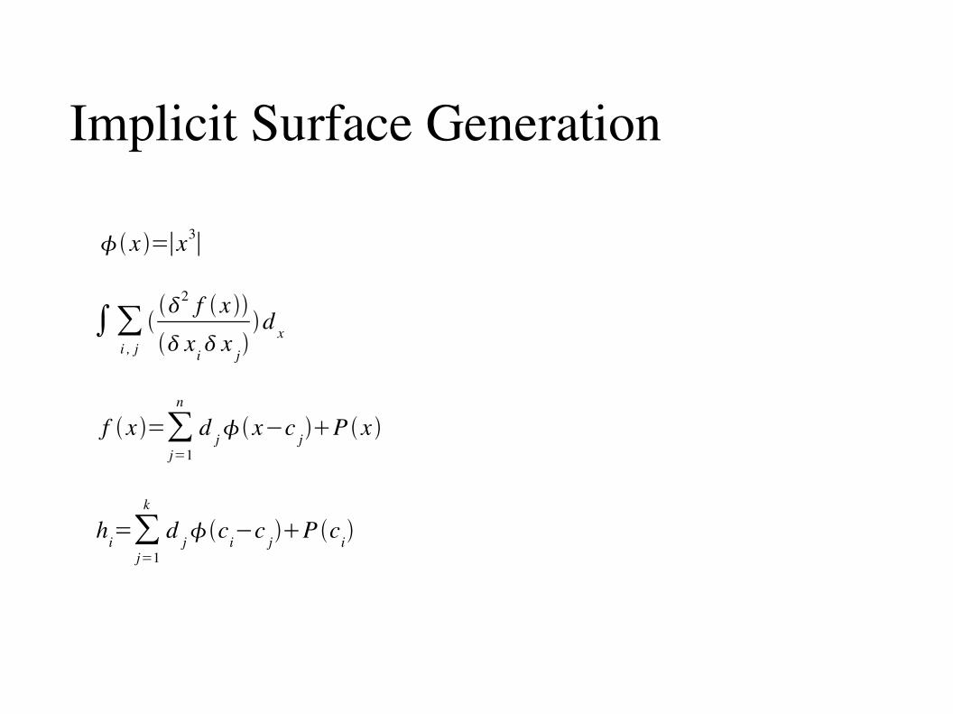
1x =∣x3∣
● Surface is described by a weighted set of radial basis functions– One function for each constraint – Basis function (1) is chosen to minimize local curvature (2)
● High local curvature complicates solution of linear system to determine weights of basis functions
● Not sure why choice of |x3| minimizes the curvature
Implicit Surface Generation
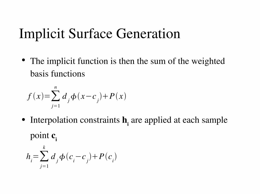
f x =∑j=1
n
d jx−c jP x
hi=∑j=1
k
d jci−c jP ci
● The implicit function is then the sum of the weighted basis functions
● Interpolation constraints hi are applied at each sample point ci
Implicit Surface Generation
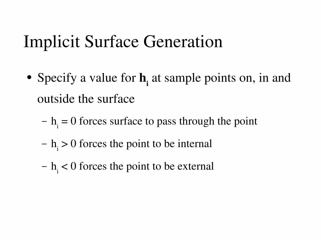
● Specify a value for hi at sample points on, in and outside the surface– hi = 0 forces surface to pass through the point
– hi > 0 forces the point to be internal
– hi < 0 forces the point to be external
Implicit Surface Generation
〚11 12 ... 1 k 1 c1
x c1y c1
z
21 22 ... 1 k 1 c2x c2
y c2z
: : : : : : : : :k1 k2 ... kk 1 ck
x cky ck
z
1 1 ... 1 0 0 0 0c1
x c2x ... ck
x 1 0 0 0
c1y c2
y ... cky 1 0 0 0
c1z c2
z ... ckz 1 0 0 0
〛〚d1
d2
:d k
p0
p1
p2
p3
〛=〚h1
h2
:hk
0000
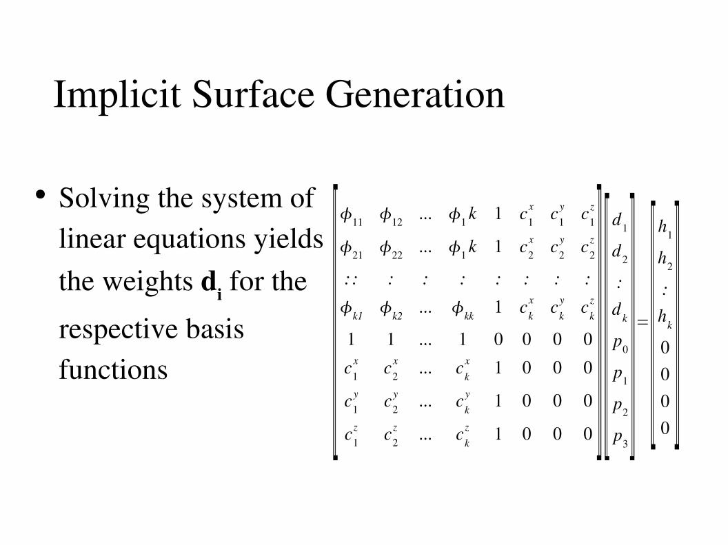
〛● Solving the system of
linear equations yields the weights di for the respective basis functions
Voxelization● Conversion from mesh to volumetric
representation– Calculated from original polygon model– High sampling density (computationally intensive)
● Each voxel is assigned a weight [0, 1]– Weight is determined by potion of the voxel
contained in the original shape– Weights vary continuously
Approximating signed distance● Identify set of boundary voxels containing
regions inside and outside the polygon model
– this is the set ∂fgoal ● Compute approximate signed euclidean distance
from each voxel to nearest boundary– Treat voxels as 6connected graph, compute the
shortest path to the boundary
Evaluating Isosurface Fit
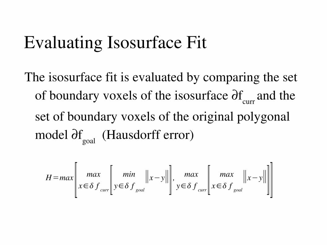
H=max 〚 maxx∈ f curr 〚 min
y∈ f goal
∥x−y∥〛 , maxy∈ f curr 〚 max
x∈ f goal
∥x−y∥〛〛
The isosurface fit is evaluated by comparing the set of boundary voxels of the isosurface ∂fcurr and the set of boundary voxels of the original polygonal model ∂fgoal (Hausdorff error)
Evaluating Isosurface Fit with Original Model
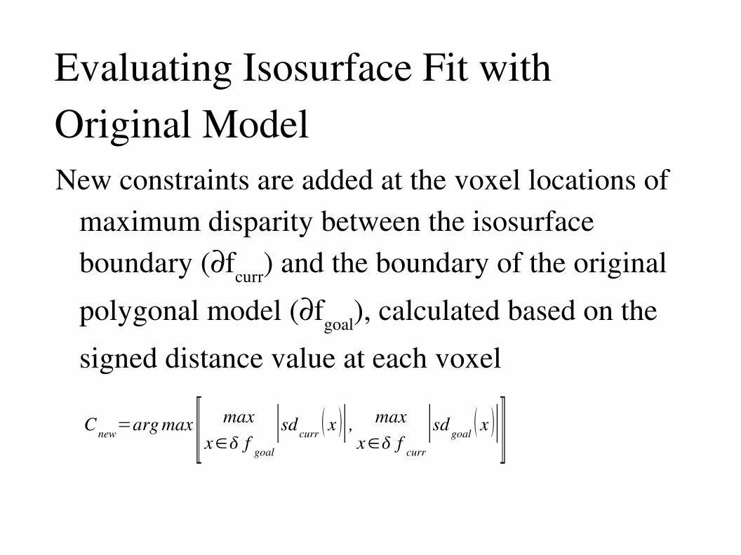
C new=arg max 〚 maxx∈ f goal
∣sd curr x ∣, maxx∈ f curr
∣sd goal x ∣〛
New constraints are added at the voxel locations of maximum disparity between the isosurface boundary (∂fcurr) and the boundary of the original polygonal model (∂fgoal), calculated based on the signed distance value at each voxel

Initial Boundary Constraints● Random choice of initial constraint locations● Poisson distribution:
– Points are added randomly– Distribution is globally uniform, but unconstrained– In subregions, some neighboring samples close
together, some far apart
Initial Boundary Constraints● Poisson disc distribution:
– Same as Poisson distribution, but imposes minimumdistance constraint between samples
– Applied using unsigned euclidean distance– Points are added at random, but removed if they
violate distance constraint– Guarantees an even sample distribution
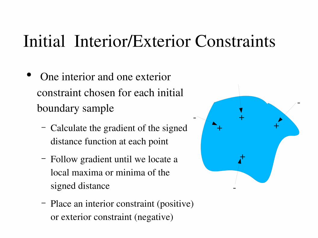
Initial Interior/Exterior Constraints● One interior and one exterior
constraint chosen for each initial boundary sample– Calculate the gradient of the signed
distance function at each point– Follow gradient until we locate a
local maxima or minima of the signed distance
– Place an interior constraint (positive) or exterior constraint (negative)
++
+
+
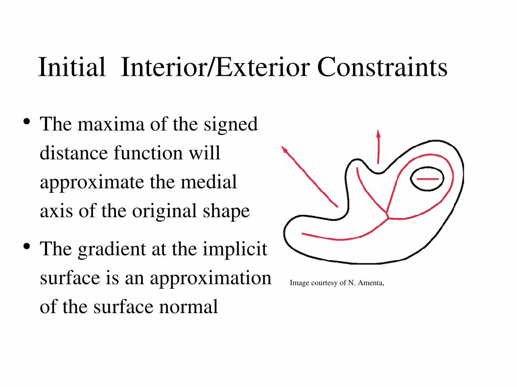
Initial Interior/Exterior Constraints● The maxima of the signed
distance function will approximate the medial axis of the original shape
● The gradient at the implicit surface is an approximation of the surface normal
Image courtesy of N. Amenta,

Adding Constraints● Volume is coarsely sampled
– Interior voxels sampled randomly/sparsely– Boundary voxels sampled at full voxel resolution
● Any 4x4 cube intersecting isosurface boundary or model boundary fully sampled
● Any 4x4 cube within 8 voxels of model boundary is fully sampled
Adding Constraints● Hausdorff Error is calculated for all voxels in the
isosurface and model boundary set– New constraint added at voxel with maximum error
(greedy algorithm)– Apply boundary constraint (0) if voxel is in model
boundary– Apply interior/exterior constraint if voxel is on
isosurface boundary
Adding Constraints● Overconstraining the system will produce erratic
results– Enforce a separation between constraint locations of
2x the abs. value of the signed distance– This ensures that spheres enclosing each constraint
with radius = signed distance at x will not overlap (same idea as Poisson disc dist. in initial sampling)
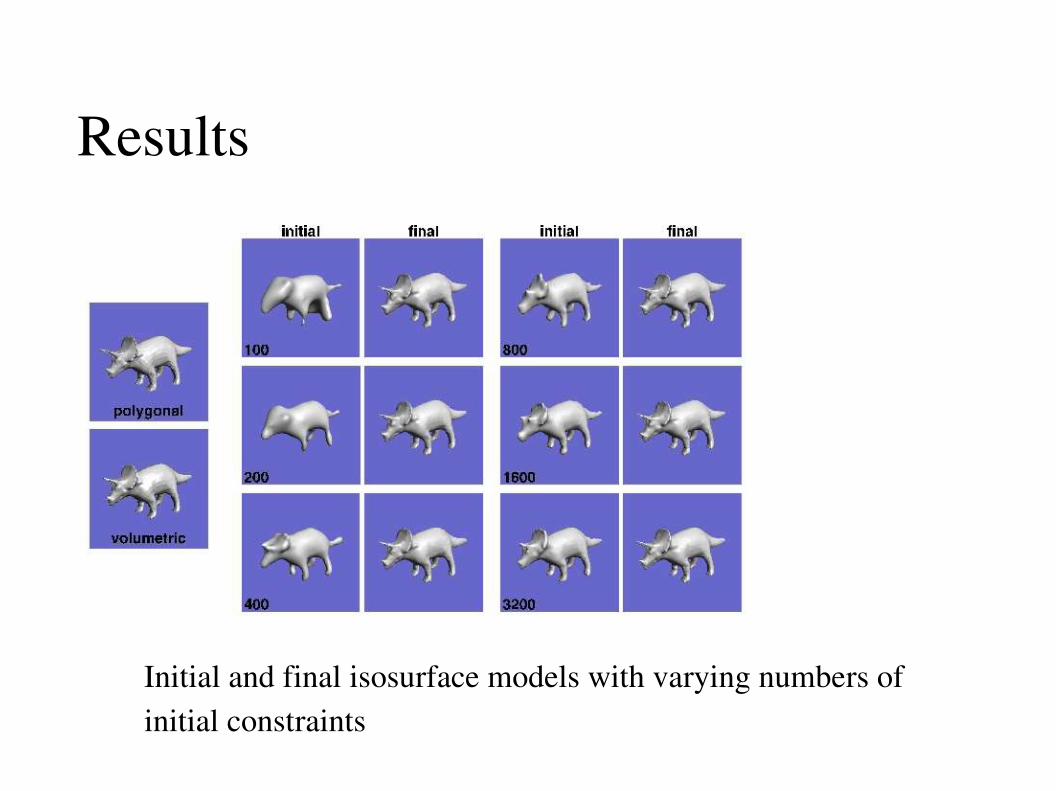
Results
Initial and final isosurface models with varying numbers of initial constraints
Results
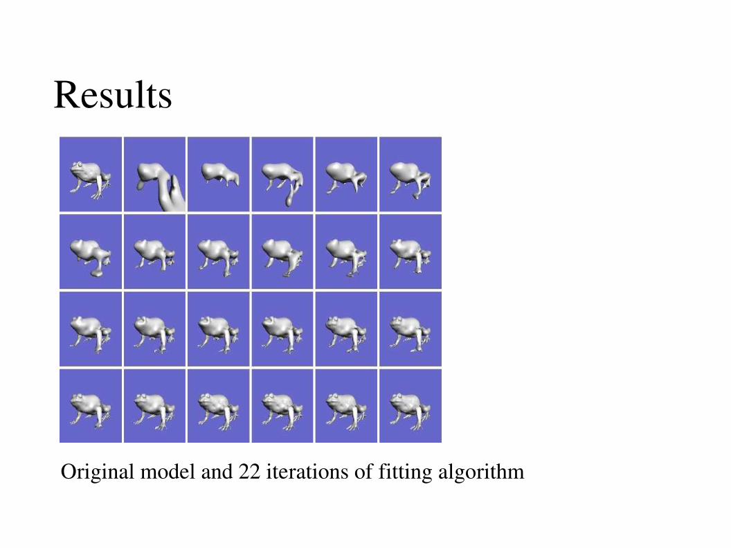
Original model and 22 iterations of fitting algorithm
Results
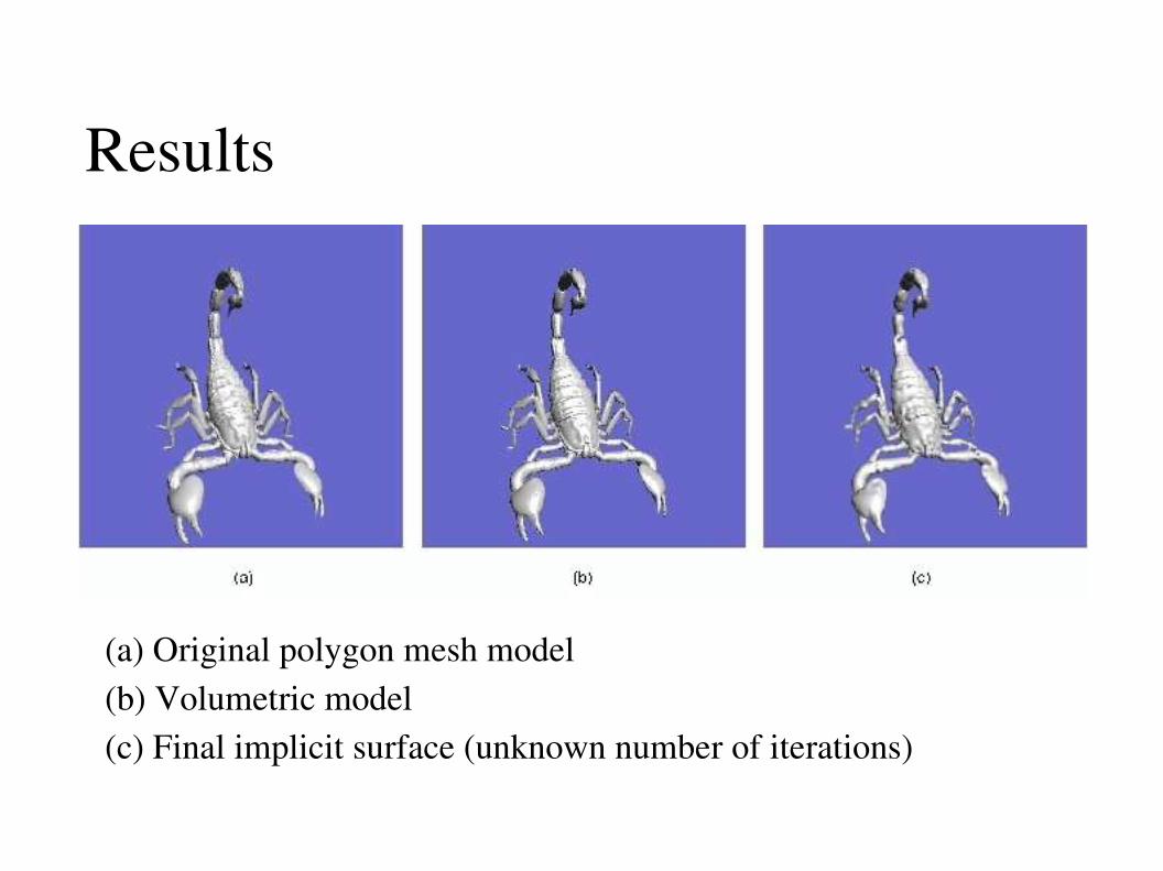
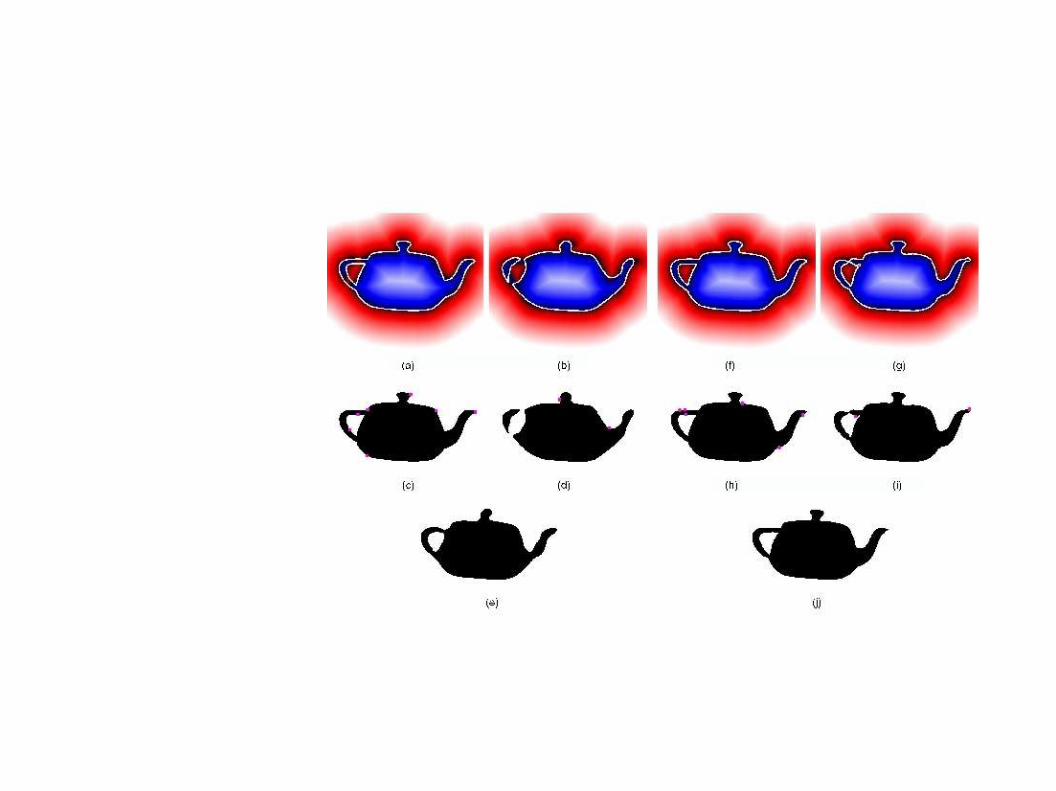
(a) Original polygon mesh model(b) Volumetric model(c) Final implicit surface (unknown number of iterations)
Sample Results
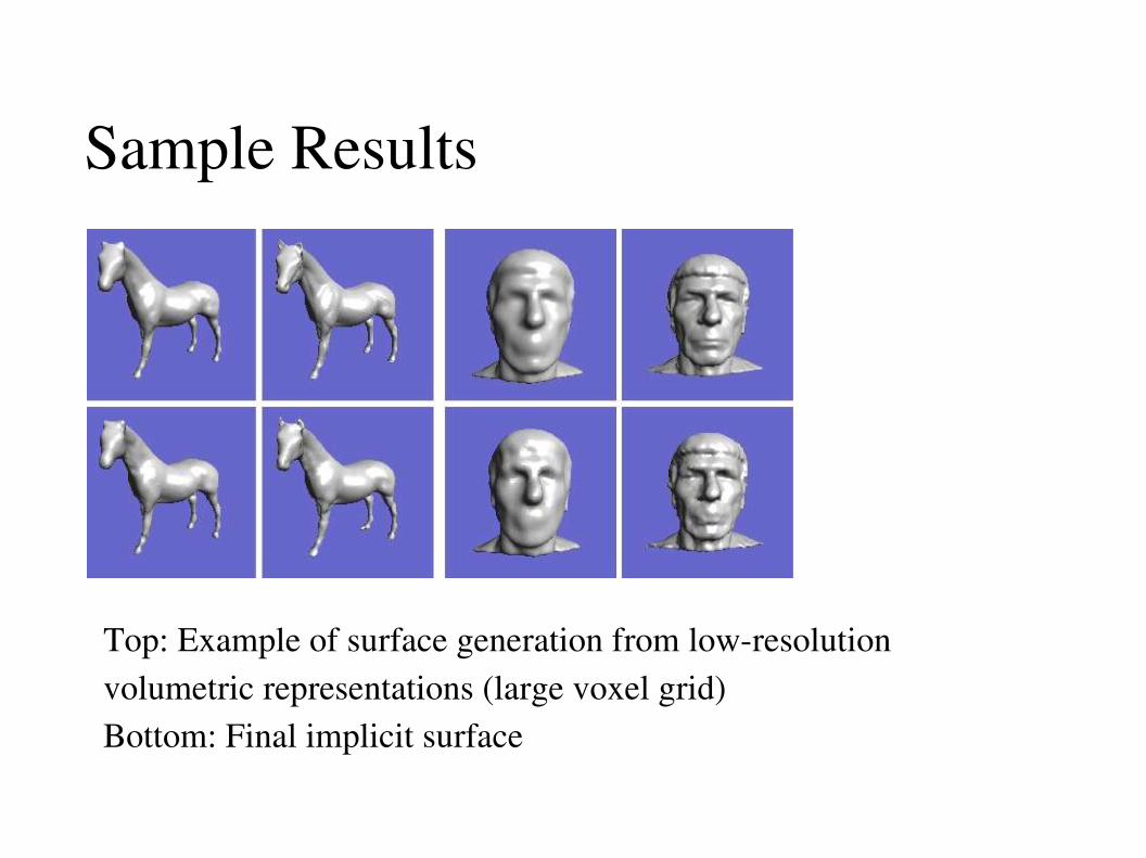
Top: Example of surface generation from lowresolution volumetric representations (large voxel grid)Bottom: Final implicit surface
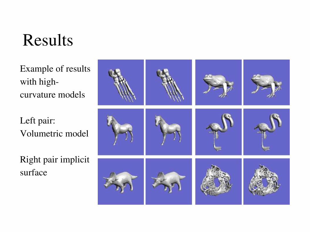
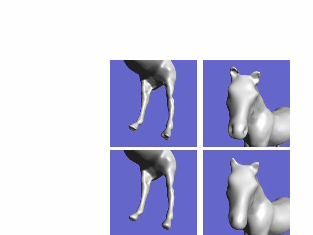
ResultsExample of results with highcurvature models
Left pair: Volumetric model
Right pair implicit surface
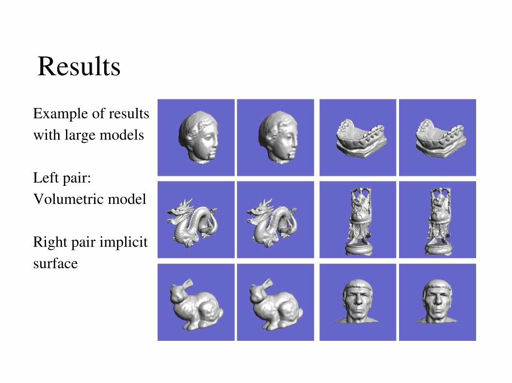
ResultsExample of results with large models
Left pair: Volumetric model
Right pair implicit surface
END
Implicit Surface Generation
∫∑i , j
2 f x x i x j
d x
f x =∑j=1
n
d jx−c jP x
hi=∑j=1
k
d jci−c jP ci
x =∣x3∣