Fitting Smooth Surfaces to Dense Polygon MeshesVenkat Krishnamurthy

Marc LevoyComputer Science Department

Stanford University

Abstract

Recent progress in acquiring shape from range data permits the ac-quisition of seamless million-polygon meshes from physical mod-els. In this paper, we present an algorithm and system for convert-ing dense irregular polygon meshes of arbitrary topology into ten-sor product B-spline surface patches with accompanying displace-ment maps. This choice of representation yields a coarse but effi-cient model suitable for animation and a fine but more expensivemodel suitable for rendering.

The first step in our process consists of interactively paintingpatch boundaries over a rendering of the mesh. In many applica-tions, interactive placement of patch boundaries is considered partof the creative process and is not amenable to automation. The nextstep is gridded resampling of each boundedsection of the mesh. Ourresampling algorithm lays a grid of springs across the polygon mesh,then iterates between relaxing this grid and subdividing it. This gridprovides a parameterization for the mesh section, which is initiallyunparameterized. Finally, we fit a tensor product B-spline surface tothe grid. We also output a displacement map for each mesh section,which represents the error between our fitted surface and the springgrid. These displacement maps are images; hence this representa-tion facilitates the use of image processing operators for manipulat-ing the geometric detail of an object. They are also compatible withmodern photo-realistic rendering systems.

Our resampling and fitting steps are fast enough to surface a mil-lion polygon mesh in under 10 minutes - important for an interactivesystem.

CR Categories: I.3.5 [Computer Graphics]: Computational Geom-etry and Object Modeling —curve, surface and object representa-tions; I.3.7[Computer Graphics]:Three-Dimensional Graphics andRealism—texture; J.6[Computer-Aided Engineering]:Computer-Aided Design (CAD); G.1.2[Approximation]:Spline Approxima-tion

Additional Key Words: Surface fitting, Parameterization, Densepolygon meshes, B-spline surfaces, Displacement maps

Authors’ Address: Department of Computer Science, Stanford University,Stanford, CA 94305

E-mail: venkat,levoy@cs.stanford.eduWorld Wide Web: http://www-graphics.stanford.edu/�venkat,�levoy

1 IntroductionAdvances in range image acquisition and integration allow us tocompute geometrical models from complex physical models [9, 36].The output of these technologies is a dense, seamless (i.e. mani-fold) irregular polygon mesh of arbitrary topology. For example,the model in figure 12, generated from 75 scans of an action figureusing a Cyberware laser range scanner, contains 350,000 polygons.Models like this offer new opportunities to modelers and animatorsin the CAD and entertainment industries.

Dense polygon meshes are an adequate representation for someapplications. Several commercial animation houses employ poly-gon meshes almost exclusively. However, for reasons of compact-ness, control, manufacturability, or appearance, many users prefersmooth surface representations. To satisfy these users, techniquesare needed for fitting surfaces to dense meshes of arbitrary topology.

A notable property of these new acquisition techniques is theirability to capture fine surface detail. Whatever fitting technique weemploy should strive to retain this fine detail. Surprisingly, a unifiedsurface representation may not be the best approach. First, the heavymachinery of most smooth surface representations (for example B-splines) makes them an inefficient way to represent fine geometricdetail. Second and perhaps more important, although geometric de-tail is useful at the rendering stage of an animation pipeline, it maynot be of interest to either the modeler or the animator. Moreover,its presence may degrade the time or memory performance of themodeling system. For these reasons, we believe it is advantageousto separate the representations of coarse geometry and fine surfacedetail.

Within this framework, we may choose from among many rep-resentations for these two components. For representing coarsegeometry, modelers in the entertainment and CAD industry havelong used NURBS [14] and in particular uniform tensor product B-splines. Such models typically consist of control meshes stitchedtogether to the level of continuity desired for an application. In or-der to address their needs we have chosen uniform tensor productB-splines as our surface representation.

For representing surface detail, we propose using displacementmaps. Each pixel in such a map gives an offset from a point ona fitted surface to a point on a gridded resampling of the originalpolygon mesh. The principal advantageof this representation is thatdisplacement maps are essentially images. As such, they can beprocessed, retouched, compressed, and otherwise manipulated us-ing simple image processing tools. Some of the effects shown infigures 11 and 13 were achieved using Adobe Photoshop, a com-mercial photo retouching program.

1.1 System overview

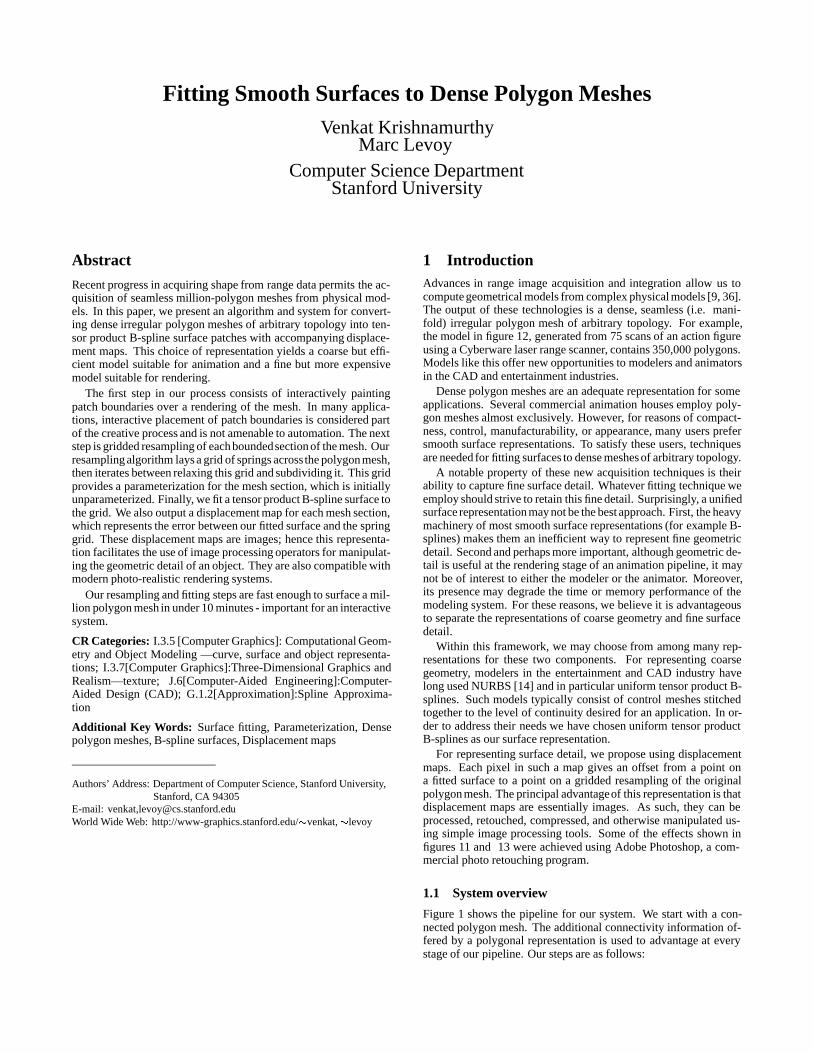
Figure 1 shows the pipeline for our system. We start with a con-nected polygon mesh. The additional connectivity information of-fered by a polygonal representation is used to advantage at everystage of our pipeline. Our steps are as follows:

Physical model.

Dense,irregular polygon mesh.

Polygonalpatches.

Per patch spring meshes.

Set of stitchedB−Splinecontrol meshes.

Set of associated displacement maps.

Scan and integrate

Paintboundarycurves

Automaticallyresample intoregular grid Fit Surface

Figure 1. Our surface fitting pipeline: the input to our system is a dense irregular polygon mesh. First, boundary curves for the desired spline patchesare painted on the surface of the unparameterized model. The output of this step is a set of boundedmesh regions. We call each such region a polygonalpatch. We next perform an automated resampling of this polygonal patch to form a regular grid that lies on the surface of the polygonal patch. Wecall this regular grid a spring mesh. Finally, we fit surfaces to the spring mesh and output both a B-spline surface representation and a set of associateddisplacement maps to capture the fine detail.

1. Our first step is an interactive boundary curve painting phasewherein a modeler defines the boundaries of a number ofpatches. This is accomplished with tools that allow the paint-ing of curves directly on the surface of the unparameterizedpolygonal model. Here, the connectivity of the polygon meshallows the use of local graph search algorithms to make curvepainting operations rapid. This property is useful when amodeler wishes to experiment with different boundary curveconfigurations for the same model. Each region of the meshthat a B-spline surface must be fit to is called a polygonalpatch. Since patch boundaries have been placed for artisticreasons, polygonal patches are not constrained to be heightfields. Our only assumptions about them are that each is arectangularly parameterizable piece of the surface that has noholes.

2. In the next step we generate a gridded resampling for eachpolygonal patch. This is accomplished by an automaticcoarse-to-fine resampling of the patch, producing a regulargrid that is constrained to lie on the polygonal surface. Wecall this grid the spring mesh. Its purpose is to establisha parameterization for the unparameterized surface. Ourresampling algorithm is a combination of relaxation andsubdivision steps that iteratively refine the spring mesh at agiven resolution to obtain a better sampling of the underlyingpolygonal patch. This refinement is explicitly directed bydistortion metrics relevant to the spline fit. The output of thisstep is a fine gridding of each polygonal patch in the model.

3. We now use standard gridded data fitting techniques to fit a B-spline surface to the spring mesh corresponding to each polyg-onal patch. The output of this step is a set of B-spline patchesthat represent the coarse geometry of the polygonal model. Torepresent fine detail, we also compute a displacement map foreach patch as a gridded resampling of the difference betweenthe spring mesh and the B-spline surface. This regular sam-pling can conveniently be represented as a vector (rgb) imagewhich stores a 3-valued displacement at each sample location.Each of these displacements represents a perturbation in thelocal coordinate frame of the spline surface. This image repre-sentation lends itself to a variety of interesting image process-ing operations such as compositing, painting, edge detectionand compression. An issue in our technique, or in any tech-nique for fitting multiple patches to data is ensuring continu-ity between the patches. We use a combination of knot linematching and a stitching post-process which together give usG1 continuity everywhere. This solution is widely used in theentertainment industry.

The remainder of this paper is organized as follows. Section2 reviews relevant previous work. Section 3 describes our tech-niques for painting boundary curves over polygonal meshes. Sec-tion 4 presents our coarse-to-fine, polygonal patch resampling algo-rithm and the surface fitting process. Section 5 describes our strat-egy for extracting displacement maps and some interesting applica-tions thereof. Section 6, discusses techniques for dealing with con-tinuity across patch boundaries. Finally, section 7 concludes by dis-cussing future work.

Throughout this paper we will draw on examples from the enter-tainment industry. However, our techniques are generally applica-ble.

2 Previous workThere is a large literature on surface fitting techniques in the CAD,computer vision and approximation theory fields. We focus here ononly those techniques from these areas that use dense (scanned) dataof arbitrary topology to produce smooth surfaces. We can classifysuch surface fitting techniques as manual, semi-automated and au-tomated.

2.1 Manual techniquesManual approachescan be divided into two categories. The first cat-egory includes all methods for digitizing a physical model directly.For example, using a touch probe, one can acquire only data that isrelevant to the final surface model. Catalogues of computer mod-els published by ViewPoint Data Labs and the work of Pixar’s ani-mation group [24, 28] exemplify these methods. These methods in-volve human intervention throughout the data acquisition processand are hence time-consuming, especially if the model is complexor the data set required is large. In contrast, our pipeline employsautomatic data acquisition methods [9].

The second category uses scanned data as a template to assistin the model construction process. Point cloud or triangulated datais typically imported into a conventional modeling system. A userthen manually projects isolated points to this data as a means of de-termining the locations of control points (or edit points [15]) forsmooth parametric surfaces. These methods require less human in-tervention than those in the first category but complex models maystill require a lot of labour.

2.2 Semi-automated techniquesThe approaches in this category take point cloud data sets as input.Examples include commercial systems such as Imageware’s Sur-facer [33], Delcam’s CopyCAD, and some research systems [20,22]. These approaches begin by identifying a subset of points that

are to be approximated. Parameterization of data points is usu-ally accomplished by a user-guided process such as projection ofthe points to a manually constructed base plane or surface. A con-strained, non-linear least squares problem is then solved on this sub-set of the point cloud to obtain a B-spline surface for the specifiedregion. While point cloud techniques are widely applicable, theyfail to exploit topological information already present in the inputdata. As demonstrated by Curless et al [9] and Turk et al [36], us-ing this additional information can significantly improve quality ofreconstruction. In the context of our surface fitting algorithm, work-ing with connectedpolygonal representations has also facilitated thedevelopment of an automatic parameterization scheme.

2.3 Automated surface fitting techniquesEck et al [12] describe a method for fitting irregular meshes with anumber of automatically placed bicubic Bezier patches. For the pa-rameterization step, a piecewise linear approximation to harmonicmaps [11] is used, and the number of patches is adjusted to achievefitting tolerances. While this method produces high quality surfaces,it includes a number of expensive optimization steps, making it tooslow for an interactive system. Further, their technique does not sep-arate fine geometric detail from coarse geometry. Particularly forvery dense meshes, we find this separation both useful and prefer-able, as already explained. We compare some other aspects of theparameterization scheme of Eck et al [11] with ours in section 4.10.

We briefly mention some techniques [29, 31] that use hierarchi-cal algorithms to fit parametric surfaces to scanned data sets. Whilethese approaches work well for regular data, they do not addressthe problem of unparameterized, irregular polygon meshes. Finally,Sclaroff et al [32] demonstrate the use of displacement maps inthe context of interpolating data with generalized implicit surfaces.However, this method also works only on regular data sets.

2.4 Relevant work in texture mappingA key aspect of our method is an automatic parameterizationscheme for irregular polygon meshes. As such, there are techniquesin the texture mapping literature that address similar problems, no-tably the work of Bennis et al [6] and that of Maillot et al [21]. Bothof these papers present schemes to re-parameterize surfaces for tex-ture mapping. These algorithms work well with regular data sets,such as discretized splines. However, they can exhibit objection-able parametric distortions in general [11]. Pedersen [25] describesa method for texture mapping (and hence parameterizing) implicitsurfaces. While the methods work well with implicit surfaces, theyrely on smoothness properties of the surface and require the evalua-tion of global surface derivatives. Irregular polygon meshes in gen-eral, are neither smooth nor conducive to the evaluation of globalsurface derivatives, as discussed by Welch et al [38].

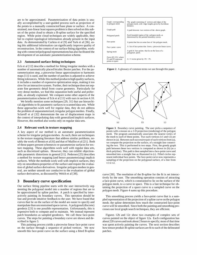
3 Boundary curve specificationOur surface fitting pipeline starts with the user interactively seg-menting the polygonal model into a number of regions that are tobe approximated by spline patches. A patch is specified by inter-actively painting its boundary curves. This operation should befast and provide intuitive feedback to the user. We have found thatcurves that lie on the surface of the model are easier to specify andmanipulate than unconstrained spacecurves. A polygonal (discrete)geodesic [23] is one possible representation. Unfortunately, this isexpensive both to compute and to maintain. We instead representpatch boundaries as sampled geodesics. We call these face-pointcurves. The steps for painting a boundary curve are shown and de-scribed in figure 3.

This painting process yields a piecewise linear face-point curveon the surface through a sequence of picked vertices. We nowsmooth this face-point curve on the surface using a fitted B-spline

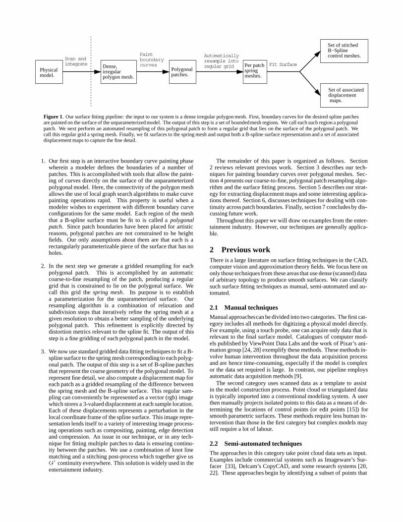
Graph correspondingto polygon mesh

Polygonal patch

Face point

Force (P2, P1) whereP1 and P2 representpoints in space

The graph consisting of vertices and edges of the polygon mesh, with edge lengths given by Euclidean distance.

Each bounded region of the polygon mesh, as determined by the painted boundary curves.

A point that lies on some face of the polygon mesh.

Spring mesh A grid of face points that lie on the faces of apolygonal patch.

A 3−vector given by P2 − P1.

Face−point curve A list of face points that form a piecewise linear curve.

Graph path A path between two vertices of the above graph.

Figure 2. A glossary of common terms we use through this paper.

(a) (b) (c)

v1

v2

Figure 3. Boundary curve painting. The user picks a sequence ofpoints with a mouse on a 2-D projection (rendering) of the polygonmesh. The program automatically associates the nearest vertex ofthe mesh to each of these points. Two such vertices (v1 and v2) areshown in (a). Between each successivepair of such vertices from (a),we compute the projection on the surface, of a straight line connect-ing the two. This is performed in two steps. First, the greedy graphpath between these two vertices is computed as shown in (b) (as athick polyline). This path is then sampled into a face-point curve andsmoothed into a straight line as illustrated in (c). Filled circles rep-resent individual face points. The face-point curve now represents asampling of the projection on the polygonal surface, of a line fromv1 to v2.

curve [30]. The resolution of the B-spline for the fit is set interac-tively by the user. The smoothing operation consists of attractinga face-point curve, which is constrained to lie on the surface of thepolygon mesh, to a curve in space. This is a fast technique for ob-taining the projection of a space curve to a sampled curve on thepolygon mesh. Figure 4 sums up this procedure.

This smoothing process yields a face-point curve that is a sam-pled representation of the projection of a spline curve on the polygonmesh; the spline determines how much the constructed face-pointcurve will be smoothed. Since both the painting and smoothing pro-cesses use local graph search techniques, they are efficient.

Figures 12b and 12c show two examples of complex sets ofcurves painted on the object of figure 12a. Each configuration hasabout 220 curves and took about 2 hours to specify; most of that timewas spent actively painting the curves. The next section describeshow tensor product B-spline surfaces are fit to each of the delineatedpatches.

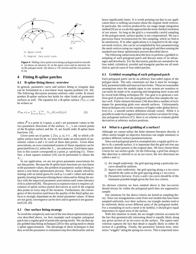
Ae

Ar

v

S: Space curve

F: Sampled face po int curve

(a) (b)

rest positionof Ae

F

Ae

Ar

S

Figure 4. Sliding a face-point curvealong a polygonmesh to smoothit. (a) shows an attractor Ar on the space curve and an attractee Aeon the polygon mesh. (b) shows a 1-D version and the rest positionof Ae.

4 Fitting B-spline patches4.1 B-spline fitting theory: overviewIn general, parametric curve and surface fitting to irregular datacan be formulated as a non-linear least squares problem [10, 30].The following discussion assumes uniform cubic (order 4) tensorproduct B-spline surfaces but holds for other kinds of parametricsurfaces as well. The equation for a B-spline surface ~P (u; v) canbe written as:

~P (u; v) =Pn

i=0

Pm

j=0Xi;jBi(u)Bj(v) (1)

where ~P is a point in 3-space, u and v are parameter values in thetwo parametric directions of the surface, Xi;j’s are control pointsof the B-spline surface and the Bi are fourth order B-spline basisfunctions [4] .

Given some set of points f ~pl(x, y, z), l=1 ...Mg to which a B-spline surface must be fit, we must first make an association of pa-rameter values u and v to each of these data points. Given theseassociations, an over-constrained system of linear equations can begenerated from (1), where theXi;j are unknowns. Each linear equa-tion in this system corresponds to a point ~pl satisfying (1). There-fore, a least squares solution [19] can be performed to obtain theXi;j .

In our application, we are not given parameter associations forour data points. Because the B-spline basis functions are non-linearin the parameter values, the problem of parametric surface fitting re-quires a non-linear optimization process. This is usually solved bystarting with an initial guess for each pl’s u and v values and subse-quently iterating between refining these values and re-fitting the sur-face with the improved parameter associations until some toleranceof fit is achieved [30]. This process is expensivesince it requires cal-culation of spline surface partial derivatives at each of the originaldata points at every step of the iteration. Furthermore, the conver-gence of this iteration (and hence the quality of the fitted spline sur-face) is strongly dependant on the initial parameter values. If theseare not good, convergence can be slow and in general is not guaran-teed [18, 20].

4.2 Our surface fitting strategyTo avoid the complexity and cost of the non-linear optimization pro-cess described above, we first resample each irregular polygonalpatch into a regular grid of points (the spring mesh). We can then ap-ply gridded data fitting techniques [29] to this spring mesh to obtaina spline approximation. The advantage of these techniques is thatthey avoid the parameter re-estimation step described earlier and are

hence significantly faster. It is worth pointing out that in our appli-cation there is nothing sacrosanct about the original mesh vertices.In particular, the vertices produced by our range image integrationmethod [9] are at a scale that approaches the noise-limited resolutionof our sensor. As long as the grid is a reasonably careful samplingof the polygon mesh, surface quality is not compromised. We use apiecewise linear reconstruction for this sampling, which we find tobe satisfactory. If in other applications it is required to fit the origi-nal mesh vertices, this can be accomplished by first parameterizingthe mesh vertices using our regular spring grid and then running thestandard non-linear optimization process described above.

The following subsections describe how to perform a gridded re-sampling of each polygonal patch and discuss some of its advan-tages and drawbacks. For the discussion, patches are assumed to befour sided; cylindrical, toroidal and triangular patches are all mod-eled as special cases of four-sided patches.

4.3 Gridded resampling of each polygonal patchEach polygonal patch can be an arbitrary four-sided region of thepolygon mesh. The only constraints are that it must be rectangu-larly parameterizable and must not have holes. These are reasonableassumptions since the models input to our system are seamless orcan easily be made so by acquiring and integrating more scans andby recent hole-filling techniques [9]. Our goal is to generate a uni-form grid of points over the polygonal surface that samples the sur-face well. Finite element literature [34] describes a number of tech-niques for generating grids over smooth surfaces. Unfortunately,these techniques rely on the existence of higher order global deriva-tives (i.e. a smooth surface definition already exists). While it ispossible to make local approximations to surface curvature for irreg-ular polygonal surfaces [37], there is no scheme to evaluate globalderivatives at arbitrary surface positions.

4.4 What is a good gridding of a surface?Although we cannot utilize the finite element literature directly, itoffers useful insight on objective functions one might minimize toproduce different surface parameterizations.

Since each polygonal patch is resampled into a regular grid in or-der to fit a smooth surface, it is important that the grid not lose anygeometric detail present in the original data. We have chosen threecriteria for our surface grids: (In the following, a grid line along ei-ther direction is referred to as an iso-curve; the two directions arecalled u and v.)

1) Arc length uniformity: the grid spacing along a particular iso-curve should be uniform.

2) Aspect ratio uniformity: the grid spacing along a u iso-curveshould be the same as the grid spacing along a v iso-curve.

3) Parametric fairness: Every u and v iso-curve should be of theminimum possible length given the first two criteria.

An obvious criterion we have omitted above is that iso-curvesshould always lie within the polygonal patch they are supposed tosample.

Our intuitions for the above criteria are based on sampling the-ory. Since our triangulations come from real models that have beensampled uniformly over their surfaces, our triangle meshes tend tobe uniformly dense across different parts of the polygonal model.For a resampling of such a mesh to be faithful, it should give equalimportance to equal areas of the surface.

With this intuition in mind, the arc-length criterion accounts forthe fact that geometrically interesting detail is equally likely alongany given section of an iso-curve on the surface. The aspect-ratiocriterion captures the fact that detail is equally likely in either di-rection of a gridding. Finally, the parametric fairness term, mini-mizes “wiggles” along the spring iso-curves. This is important since

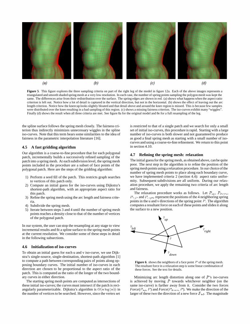
Figure 5. This figure explores the three sampling criteria on part of the right leg of the model in figure 12a. Each of the above images represents atriangulated and smooth shaded spring mesh at a very low resolution. In each case, the number of spring points sampling the polygon mesh was kept thesame. The differences arise from their redistribution over the surface. The spring edges are shown in red. (a) shows what happens when the aspect ratiocriterion is left out. Notice how a lot of detail is captured in the vertical direction, but not in the horizontal. (b) shows the effect of leaving out the arclength criterion. Notice how the kneecap looks slightly bloated and that detail above and around the knee region is missed. This is because few sampleswere distributed over the knee resulting in a bad sampling of this region. (c) shows a missing fairness criterion. The iso-curves exhibit many “wiggles”.Finally (d) shows the result when all three criteria are met. See figure 8a for the original model and 8e for a full resampling of the leg.

the spline surface follows the spring mesh closely. The fairness cri-terion thus indirectly minimizes unnecessary wiggles in the splineiso-curves. Note that this term bears some similarities to the idea offairness in the parametric interpolation literature [16].

4.5 A fast gridding algorithmOur algorithm is a coarse-to-fine procedure that for each polygonalpatch, incrementally builds a successively refined sampling of thepatch into a spring mesh. At each subdivision level, the spring meshpoints included in the procedure are a subset of face points of thepolygonal patch. Here are the steps of the gridding algorithm:

1) Perform a seed fill of the patch. This restricts graph searchesto vertices of this patch only.

2) Compute an initial guess for the iso-curves using Dijkstra’sshortest-path algorithm, with an appropriate aspect ratio forthis patch.

3) Refine the spring mesh using the arc length and fairness crite-ria.

4) Subdivide the spring mesh.5) Iterate between steps 3 and 4 until the number of spring mesh

points reaches a density close to that of the number of verticesof the polygonal patch.

In our system, the user can stop the resampling at any stage to viewincremental results and fit a spline surface to the spring mesh pointsat the current resolution. We consider some of these steps in detailin the following subsections.

4.6 Initialization of iso-curvesTo obtain an initial guess for each u and v iso-curve, we use Dijk-stra’s single-source, single-destination, shortest-path algorithm [1]to compute a path between corresponding pairs of points along op-posing boundary curves. The initial number of iso-curves in eachdirection are chosen to be proportional to the aspect ratio of thepatch. This is computed as the ratio of the longer of the two bound-ary curves in either direction.

The starting spring mesh points are computed as intersections ofthese initial iso-curves; the curves must intersect if the patch is rect-angularly parameterizable. Dijkstra’s algorithm is O(n log(n)) inthe number of vertices to be searched. However, since the vertex set

is restricted to that of a single patch and we search for only a smallset of initial iso-curves, this procedure is rapid. Starting with a largenumber of iso-curves is both slower and not guaranteed to produceas good a final spring mesh as starting with a small number of iso-curves and using a coarse-to-fine refinement. We return to this pointin section 4.10.

4.7 Refining the spring mesh: relaxationThe initial guess for the spring mesh, as obtained above, can be quitepoor. The next step in the algorithm is to refine the position of thespring mesh points using a relaxation procedure. In our choice of thenumber of spring mesh points to place along each boundary curve,we have implemented criteria 2 (section 4.4): aspect ratio unifor-mity. Subsequent subdivisions are all uniform. During our relax-ation procedure, we apply the remaining two criteria of arc lengthand fairness.

The relaxation procedure works as follows. Let Pup, Pdown,Pleft and Pright represent the positions of the 4 neighboring springpoints in the u and v directions of the spring point P . The algorithmcomputes a resultant force on each of these points and slides it alongthe surface to a new position.

P

P

PP

P

down

left

up

right

Figure 6. shows the neighbors of a face point P of the spring mesh.The resultant force in a relaxation step is some linear combination ofthese forces. See the text for details.

Minimizing arc length distortion along one of P ’s iso-curvesis achieved by moving P towards whichever neighbor (on thesame iso-curve) is farther away from it. Consider the two forcesForce(Pup, P ) and Force(Pdown, P ). We make the direction of thelarger of these two the direction of a new force Fud. The magnitude

ofFud is set to be the difference of the two magnitudes. We performa similar computation in the other direction (left-right) as well to geta forceFlr . Let us denote the resultant of Flr andFud byFarc. Thisresultant becomes one of the two terms in equation (2) below.

Fairness distortion is minimized by moving the point P to a po-sition that minimizes the energy corresponding to the set of springsconsisting of P andP ’s immediate neighbors along both iso-curves.This corresponds to computing a force Ffair equal to the resultantof the forces acting on P by its four neighbors: Force(Pup, P ),Force(Pdown, P ), Force(Pleft, P ) and Force(Pright, P ).

The point P is moved according to a force given by a weightedsum of Ffair and Farc:

Fresult = � � Ffair + � � Farc (2)

The relaxation iteration starts with � = 0 and � = 1 and ends with� = 1, � = 0. This strategy has proved to produce satisfactoryresults.

Note that we have used Euclidean forces in the previous step, i.e.forces that represent the vector joining two spring points. A relax-ation step based on Euclidean forces alone is fast but not guaranteedto generate good results in all cases. Figure 7a shows an examplewhere Euclidean forces alone fail to produce the desired effect.

In contrast to Euclidean forces, geodesic forces are forces alongthe surface of the mesh. These would produce the correct motionfor the spring points in the above case. One approach to solving theproblem exemplified by Figure 7a, would be to use geodesic forces,or approximations thereof, as substitutes for Euclidean forces in therelaxation step. However this is an expensive proposition since thefastest algorithm for point to point geodesics is O(n2) in the size ofthe patch [7]. Even approximations to geodesics such as local graphsearches are O(n) and would be too expensive to perform at everyrelaxation step.

A solution to the problem is motivated by figure 7b; create a newspring point Pmid�point that lies on the surface halfway betweenP1 and P2. This point generates new Euclidean forces acting onthe original points, moving them towards each other on the surface.We call this process spring mesh subdivision.

4.8 Subdividing the spring meshSpring mesh subdivision is based on a graph search and refinementalgorithm. Given two spring pointsP1 and P2 our algorithm com-putes a new face point P that is the mid-point of the two springpoints and that lies on the graph represented by the patch. The pro-cedure is:

1.) Find the two closest vertices v1 and v2 on P1 and P2’s faces.2.) Compute a breadth first graph path from v1 to v2. The mid-

point of this path serves as a first approximation to P ’s loca-tion.

3.) Refine this location by letting the forces given by Force(P1,P ) and Force(P2,P ) act onP , moving it to a new position onthe surface. This process is distinct from the relaxation pro-cess. It is used only to obtain a better approximation for P .

Subdivision along boundary curves is based on a static resam-pling of the face point curve representation; these points are nevermoved during the relaxation and subdivision steps. We terminatesubdivision when the number of spring points increases to within acertain range of the polygonal patch’s vertices.

4.9 B-spline fitting to gridded dataThe techniques described above minimize parametric distortion inthe spring mesh. In particular, they enforce minimal distortion withrespect to aspect ratio and edge lengths while ensuring parametric

P1

P2

FP1

P2

P

F

(a) (b)

V

Vmid−point

Figure 7. shows a case where relaxation alone fails to move a springmesh point in the desired direction. In each case F represents theforce on P1 from its right neighbor and V represents the resulting di-rection of motion. The desired motion of the point P1 is into the cav-ity. In (a) just the opposite occurs; the points move apart. (b) showshow this case is handled by subdividing the spring mesh along thesurface. See the text for details.

fairness. The resulting spring meshes have low area distortion aswell, as evidenced by the example shown in figure 5.

The final step in our algorithm is to perform an unconstrained,gridded data fit of a B-spline surface to each spring mesh. Aspointed out earlier, fitting to a good resampling of the data does notcompromise surface quality. We refer the reader to [29] for an ex-cellent tutorial on the subject of gridded data fitting. Figure 8 sum-marizes the sampling and fitting processes on a cylindrical patch ofthe model from figure 12.

4.10 Discussion

Our two-step approach of gridding and then fitting has several de-sirable characteristics. First, it is fast. This can be understood asfollows. At each level of subdivision, each spring mesh point musttraverse some fraction of the polygons as it relaxes. The cost of thisrelaxation thus depends linearly on size of the polygon mesh. It ob-viously also depends on the size of the spring mesh. If these twowere equal, as would occur if we immediately subdivided the springmesh to the finest level, then the cost of running the relaxation wouldbe O(n2). If, however, we employ the coarse-to-fine strategy de-scribed in the foregoing sections, then at each subdivision level, fourtimes as many spring mesh points move as on the previous (coarser)level, but they move on average half as far. Thus, the cost of relax-ation at each subdivision level is linear in the number of spring meshpoints, and the total cost due to relaxation is O(n log n). This argu-ment breaks down if we start with a large initial set of iso-curves.Similar arguments apply to the cost of subdivision.

A second advantage of our overall strategy is that it allows a userto pause the iteration at an intermediate stage and still obtain goodquality previews of the model. This is a useful property for an inter-active system, specially when dealing with large meshes. In partic-ular, subdivision to higher levels can be postponed until the modeldesigner is satisfied with a patch configuration.

A third advantage of our approach is that once the resampling isdone, the spline resolution can be changed interactively, since nofurther parameter re-estimation is necessary. We have found this tobe a useful interactive tool for a modeler, specially when making thetradeoff between explicitly represented geometry and displacementmapped detail as explained in section 5.

As mentioned earlier, there are other schemes that may be used toparameterize irregular polygon meshes. In particular, the harmonicmaps of Eck et al[11] produce parameterizations with low edge andaspect ratio distortions. However, the scheme has two main draw-backs for our purposes. First, it can cause excessive area distortionsin parameter space. Second, the algorithm employs an O(n2) itera-tion to generate final parameter values for vertices of the mesh andno usable intermediate parameterizations are produced. As pointed

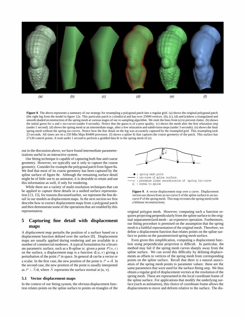
Figure 8. The above represents a summary of our strategy for resampling a polygonal patch into a regular grid. (a) shows the original polygonal patch(the right leg from the model in figure 12a. This particular patch is cylindrical and has over 25000 vertices. (b), (c), (d) and (e)show a triangulated andsmooth shaded reconstruction of the spring mesh at various stages of our re-sampling algorithm. We omit the lines from (e) to prevent clutter. (b) showsthe initial guess for u and v iso-curves (under 4 seconds). Notice that the guess is of a poor quality. (c) shows the mesh after the first relaxation step(under 1 second). (d) shows the spring mesh at an intermediate stage, after a few relaxation and subdivision steps (under 3 seconds). (e) shows the finalspring mesh without the spring iso-curves. Notice how the fine detail on the leg was accurately captured by the resampled grid. This resampling took23 seconds. All times are on a 250 Mhz Mips R4400 processor. (f) shows a spline fit that captures the coarse geometry of the patch. This surface has27x36 control points. It took under 1 second to perform a gridded data fit to the spring mesh of (e).

out in the discussion above, we have found intermediate parameter-izations useful in an interactive system.

Our fitting technique is capable of capturing both fine and coarsegeometry. However, we typically use it only to capture the coarsegeometry. Consider for example the polygonal patch from figure 8a.We find that most of its coarse geometry has been captured by thespline surface of figure 8e. Although the remaining surface detailmight be of little use to an animator, it is desirable to retain and usethis information as well, if only for rendering.

While there are a variety of multi-resolution techniques that canbe applied to capture these details in a unified surface representa-tion [13, 15], for reasons discussed earlier, we represent the fine de-tail in our models as displacement maps. In the next section we firstdescribe how to extract displacement maps from a polygonal patchand then demonstrate some of the operations that are enabled by thisrepresentation.

5 Capturing fine detail with displacementmaps

A displacement map perturbs the position of a surface based on adisplacement function defined over the surface [8]. Displacementmaps are usually applied during rendering and are available in anumber of commercial renderers. A typical formulation for a bivari-ate parametric surface, such as a B-spline is: given a point P (u; v)on the surface, a displacement map is a function d(u; v) giving aperturbation of the point P in space. In general d can be a vector ora scalar. In the first case, the new position of the point is P + ~d. Inthe second case, the new position of the point is usually interpretedas P + N̂d, where N̂ represents the surface normal at (u, v).

5.1 Vector displacement mapsIn the context of our fitting system, the obvious displacement func-tion relates points on the spline surface to points on triangles of the

: spring mesh point : iso−curve of spli ne surface: piecewise linear reconstruction of spring iso−curve: normal to spline

N̂

N̂

Figure 9. A vector displacement map over a curve. Displacementvectors are shown from an iso-curve S of the spline surface to an iso-curve P of the spring mesh. This map recreates the spring mesh (witha bilinear reconstruction).

original polygon mesh. However, computing such a function re-quires projecting perpendicularly from the spline surface to the orig-inal unparameterized mesh - an expensive operation. Furthermore,our fitting procedure is premised on the assumption that the springmesh is a faithful representation of the original mesh. Therefore, wedefine a displacement function that relates points on the spline sur-face to points on the parameterized spring mesh surface.

Even given this simplification, computing a displacement func-tion using perpendicular projection is difficult. In particular, themethod may fail if the spring mesh curves sharply away from thespline surface. We can avoid this difficulty by defining displace-ments as offsets to vertices of the spring mesh from correspondingpoints on the spline surface. Recall that there is a natural associ-ation of the spring mesh points to parameter values: these are thesame parameters that were used for the surface fitting step. We thusobtain a regular grid of displacement vectors at the resolution of thespring mesh. These are represented in the local coordinate frame ofthe spline surface. For applications that modify the underlying sur-face (such as animation), this choice of coordinate frame allows thedisplacements to move and deform relative to the surface. The dis-

placement function d(u; v) is then given by a reconstruction fromthis grid of samples. We have used a bilinear filter for the imagesshown in this paper.

Note that the displacement map is essentially a resampled errorfunction since it represents the difference of the positions of thespring points from the spline surface.

Since the displacement map, as computed, is a regular grid of 3-vectors, it can conveniently be represented as an rgb image. Thisrepresentation permits the use of a variety of image-processing op-erations such as painting, compression, scaling and compositing tomanipulate fine surface detail. Figure 11 and Figure 13 explorethese and other games one can play with displacement maps.

5.2 Scalar displacement mapsWhile vector displacement maps are useful for a variety of effects,some operations such as (displacement image) painting are more in-tuitive on grayscale images. There are several methods of arrivingat a scalar displacement image. One method is to compute a nor-mal offset from the spline surface to the spring mesh. However, asdiscussed earlier, this method is both expensive and prone to non-robustness in the presence of high curvature in the spring mesh.

Instead we have used two alternative formulations. The firstcomputes and stores at each sample location (or pixel) the magni-tude of the corresponding vector displacement. In this case, mod-ifying the scalar image scales the associated vector displacementsalong their existing directions. A second alternative, stores at eachsample location the component of the displacement vector normalto the spline surface. Modifying the scalar image therfore changesonly the normal component of the vector displacement.

Both of these last two options offer different interactions withthe displacement map. Figure 11 employs the third option - normalcomponent editing.

5.3 Bump mapsA bump map is defined as a function that performs perturbations onthe direction of the surface normal before using it in lighting calcu-lations [5]. In general, a bump map is less expensive to render thana displacement map since it does not change the geometry (and oc-clusion properties) within a scene but instead changesonly the shad-ing. Bump maps can achieve visual effects similar to displacementmaps except in situations where the cues provided by displaced ge-ometry become evident such as along silhouette edges. We computeand store bump maps using techniques very similar to those usedfor displacement maps; at each sample location instead of storingthe displacement we store the normal of the corresponding springmesh point. Figures 13d and e show a comparison of a displace-ment mapped spline and a bump mapped spline, both of which arebased on the same underlying spring mesh. Notice how, differencesare visible at the silhouette edges.

6 Continuity across patch boundariesThus far we have addressed the sampling and fitting issues con-nected with a single polygonal patch. In the presence of multiplepatches, we are faced with the problem of keeping patches continu-ous across shared boundaries and corners. If displacement maps areused, it is essential to keep the displacement mapped spline surfacecontinuous.

The extent of inter-patch continuity desired in a multi-patch B-spline (or more generally, NURBS) model depends on the domainof application. For example, in the construction of the exterior of acar body, curvature plots and reflection lines [14] are frequently usedto verify the quality of surfaces. In this context, even curvature con-tinuous (C2) surfaces might be inadequate. Furthermore, workers inthe automotive industry often use trimmed NURBS and do not nec-essarily match knot lines at shared patch boundaries during model

construction. Therefore it is not always possible to enforce math-ematical continuity across patch boundaries. Instead, statistical orvisual continuity is enforced based on user specified tolerances forposition and normal deviation. These are either enforced as linearconstraints to the fitting process[2, 33], or they are achieved throughan iterative optimization process [22].

In the animation industry, by contrast, curvature continuity isseldom required and tangent continuity (G1) usually suffices. Toachieve this the number of knots are usually forced to be the samefor patches sharing a boundary. This has several advantages. In thefirst place, control point deformations are easily propagated acrosspatch boundaries. Secondly, there is minimal distortion at bound-aries in the process of texture mapping. Finally, the process ofmaintaining patch continuity during an animation becomes easier;continuity is either made part of the model definition [24] or is re-established on a frame by frame basis using a stitching post-process.

Our system can be adapted to either of the above paradigms (i.e.either statistical or geometric continuity). Since our focus in this pa-per is on the entertainment industry, we enforce geometrical conti-nuity, and for this purpose we use a stitching post-process. Specif-ically, we allow an animator to specify the level of continuity re-quired for each boundary curve (C0 orG1). Unconstrained, griddeddata fitting to each patch leaves us with C�1 spline boundaries. Weuse end-point interpolating, uniform, cubic B-splines. To maintainmathematical continuity we constrain adjacent patches to have thesame number of control points along a shared boundary. Followingboundary conditions for these surfaces as defined by Barsky [3], C0

continuity across a shared boundary curve is obtained by averagingend control points between adjacent patches. Alternatively, G1 con-tinuity can be obtained by modifying the end control points such thatthe tangent control points (last two rows) “line up” in a fixed ratioover the length of the boundary.

Patch corners pose a harder problem. We refer the reader to [27]for a detailed account of this problem. For the kinds of basis func-tions we use, projecting the 4 corner control points of each of thepatches meeting at that corner to an average plane guarantees G1

continuity.For the case of displacement mapped splines, continuity may be

defined on the basis of the reconstruction filter used for the displace-ment maps. Recall that we generate these from the spring meshesand that we use bilinear reconstruction. Displacement mappedsplines will therefore exactly recreate the spring mesh. Also adja-cent patches can at most be position continuous with a bilinear re-construction filter. Therefore, if the spring resolutions are the sameat a shared boundary of two patches, they will be continuous byvirtue of the reconstruction. However, spring mesh resolutions candiffer across shared boundaries. This can result in occasional T-jointdiscontinuities. The problem is solved by averaging bordering rowsof displacement maps in adjacent patches. This ensures that there isno cracking at patch boundaries.

Figure 12 shows a case study of the use of our system to fit splinesurfaces, with associated displacement maps, to a large and detailedpolygonal mesh of an action figure.

7 Conclusions and future workIn conclusion, we have presented fast techniques for fitting smoothparametric surfaces, in particular tensor product B-splines, to dense,irregular polygon meshes. A useful feature of our system is that itallows incremental previewing of large patch configurations. Thisfeature is enabled by our coarse-to-fine gridded resampling schemeand proves invaluable when modelers wish to experiment with dif-ferent patch configurations of the same model. We also provide auseful method for storing and manipulating fine surface detail in theform of displacement map images. We have found that this repre-sentation empowers users to manipulate geometry using tools out-side our modeling system.

Our system has several limitations. First, becauseit relies on sur-face walking strategies and mesh connectivity to resample polygo-nal patches, it breaks down in the presence of holes in the polygonmesh. However, new range image integration techniques includemethods for filling holes.

Another limitation is that B-spline surface patches, our choice torepresent coarse geometry, perform poorly for very complex sur-faces such as draped cloth. B-splines have other disadvantages aswell, such as the inability to model triangular patches without ex-cessive parametric distortion. Despite these limitations, B-splines(and NURBS in general) are widely used in the modeling industry.This has been our motivation for choosing this over other represen-tations.

There are a number of fruitful directions for future research.Straightforward extensions include developing tools to assist inboundary curve painting and editing, improving robustness in thepresence of holes, adding further constraints to the the parameter-ization process, allowing variable knot density at the fitting stage,implementing other continuity solutions, and using adaptive springgrids for sampling decimated meshes. An example of a boundarypainting tool is a “geometry-snapping” brush that attaches curves tofeatures as the user draws on the object. Examples of constraints tothe parameterization process include interactively placed curve andpoint “attractors” within a patch.

An interesting application of the parameterization portion of oursystem is the interactive texture mapping and texture placement [26]for complex polygonal models. Related to this is the possibilityof applying procedural texture analysis/synthesis techniques [17] tocreate synthetic displacement maps from real ones. Using our tech-niques such maps can be applied to objects of arbitrary topology.

8 AcknowledgementsWe thank Brian Curless for his range image integration software,David Addleman and George Dabrowski of Cyberware for the useof a scanner, Lincoln Hu and Christian Rouet of Industrial Light andMagic for advice on the needs of animators, and Pat Hanrahan, HansPederson, Bill Lorensen for numerous useful discussions. We alsothank the anonymous reviewers for several useful comments. Thiswork was supported by the National Science Foundation under con-tract CCR-9157767 and Interval Research Corporation.

References[1] A.V.Aho and J.D.Ullman. Data structures and algorithms. Addison-Wesley,

1979.

[2] L Bardis and M Vafiadou. Ship-hull geometry representation with b-spline sur-face patches. Computer Aided Design, 24(4):217–222, 1992.

[3] Brian A. Barsky. End conditions and boundary conditions for uniform b-splinecurve and surface representations. Computers In Industry, 3, 1982.

[4] Richard Bartels, John Beatty, and Brian Barsky. An Introduction to Splines forUse in Computer Graphics and Geometric Modeling . Morgan Kaufmann Pub-lishers, Palo Alto, CA, 1987.

[5] James F. Blinn. Simulation of wrinkled surfaces. In Computer Graphics (SIG-GRAPH ’78 Proceedings) , volume 12, pages 286–292, 1978.

[6] J. Vezien Chakib Bennis and G. Iglesias. Piecewise surface flattening for non-distorted texture mapping. In Computer Graphics (SIGGRAPH’91 Proceedings) ,volume 25, pages 237–246, July 1991.

[7] Jindong Chen and Yijie Han. Shortest paths on a polyhedron. In Proc. 6th AnnualACM Symposium on Computational Geometry , pages 360–369, June 1990.

[8] Robert L. Cook. Shade trees. In Computer Graphics (SIGGRAPH ’84 Proceed-ings), volume 18, pages 223–231, July 1984.

[9] Brian Curless and Marc Levoy. A volumetric method for building complex mod-els from range images. In Computer Graphics (SIGGRAPH ’96 Proceedings) ,August 1996.

[10] Paul Dierckx. Curve and Surface Fitting with Splines . Oxford Science Publica-tions, New York, 1993.

[11] Matthias Eck, TonyDeRose, TomDuchamp, Hugues Hoppe, Michael Lounsbery,and Werner Stuetzle. Multiresolution analysis of arbitrary meshes. In ComputerGraphics (Proceedings of SIGGRAPH ’95) , pages 173–182, August 1995.

[12] Matthias Eck and Hugues Hoppe. Automatic reconstruction of b-spline surfacesof arbitrary topological type. In Computer Graphics (Proceedingsof SIGGRAPH’96), August 1996.

[13] Hugues Hoppe et al. Piecewise smooth surface reconstruction. In ComputerGraphics (Proceedings of SIGGRAPH ’94) , pages 295–302, July 1994.

[14] Gerald Farin. Curves and Surfaces for Computer Aided Geometric Design . Aca-demic Press, 1990.

[15] David R. Forsey and Richard H. Bartels. Hierarchical B-spline refinement. InComputer Graphics (SIGGRAPH ’88 Proceedings) , volume 22, pages 205–212,August 1988.

[16] Mark Halstead, Michael Kass, and Tony DeRose. Efficient, fair interpolation us-ing Catmull-Clark surfaces. In Computer Graphics (SIGGRAPH ’93 Proceed-ings), volume 27, pages 35–44, August 1993.

[17] David Heeger and James R. Bergen. Pyramid-basedtexture analysis/synthesis. InComputer Graphics (SIGGRAPH ’95 Proceedings) , pages 229–237, July 1995.

[18] J Hoschek and D Lasser. Fundamentals of Computer Aided Geometric Design .AK Peters, Wellesley, 1993.

[19] Charles L. Lawson and Richard J. Hanson. Solving Least Square Problems .Prentice-Hall, Englewood Cliffs, New Jersey, 1974.

[20] W. Ma and J P Kruth. Parameterization of randomly measured points forleast squares fitting of b-spline curves and surfaces. Computer Aided Design,27(9):663–675, 1995.

[21] Jerome Maillot. Interactivetexture mapping. In Computer Graphics (SIGGRAPH’93 Proceedings) , volume 27, pages 27–34, July 1993.

[22] M. J. Milroy, C. Bradley, G. W. Vickers, and D. J. Weir. G1 continuity of b-splinesurface patches in reverse engineering. Computer-Aided Design, 27:471–478,1995.

[23] J. S. B. Mitchell, D. M. Mount, and C. H. Papadimitriou. The discrete geodesicproblem. SIAM J. Comput., 16:647–668, 1987.

[24] Eben Ostby. Describing free-form 3d surfaces for animation. In Workshop onInteractive 3D Graphics, pages 251–258, 1986.

[25] Hans K. Pedersen. Decorating implicit surfaces. In Computer Graphics (Pro-ceedings of SIGGRAPH ’95) , pages 291–300, August 1995.

[26] Hans K. Pedersen. A framework for interactive texturing on curved surfaces. InComputer Graphics (Proceedings of SIGGRAPH ’96) , August 1996.

[27] Jorg Peters. Fitting smooth parametric surfaces to 3D data . Ph.d. thesis, Univ.of Wisconsin-Madison, 1990.

[28] William T. Reeves. Simple and complex facial animation: Case studies. In StateOf The Art In Facial Animation, SIGGRAPH course 26 , pages 90–106. 1990.

[29] David R.Forsey and Richard H. Bartels. Surface fitting with hierarchical splines.In Topics in the Construction, Manipulation, and Assessment of Spline Surfaces,SIGGRAPH course 25, pages 7–0–7–14. 1991.

[30] D. F. Rogers and N. G. Fog. Constrained b-spline curve and surface fitting. Com-puter Aided Geometric Design, 21:641–648, December 1989.

[31] Francis J. M. Schmitt, Brian A. Barsky, and Wen hui Du. An adaptive subdivi-sion method for surface-fitting from sampled data. In Computer Graphics (SIG-GRAPH ’86 Proceedings) , volume 20, pages 179–188, August 1986.

[32] Stan Sclaroff and Alex Pentland. Generalized implicit functions for computergraphics. In Computer Graphics (SIGGRAPH ’91 Proceedings) , volume 25,pages 247–250, July 1991.

[33] Sarvajit S. Sinha and Pradeep Seneviratne. Single valuedness, parameterizationand approximating3d surfaces using b-splines. Geometric Methods in ComputerVision 2, pages 193–204, 1993.

[34] J. F. Thompson. The Eagle Papers. Mississippi State University, P.O. Drawer6176, Mississippi State, MS 39762.

[35] Greg Turk. Re-tiling polygonal surfaces. In Computer Graphics (SIGGRAPH’92 Proceedings) , volume 26, pages 55–64, July 1992.

[36] Greg Turk and Marc Levoy. Zippered polygon meshes from range images. InComputer Graphics (SIGGRAPH ’94 Proceedings) , pages 311–318, July 1994.

[37] William Welch and Andrew Witkin. Free–Form shape design using triangulatedsurfaces. In Computer Graphics (Proceedings of SIGGRAPH ’94) , pages 247–256, July 1994.

[38] William Welch and Andrew Witkin. Free-form shape design using triangulatedsurfaces. In Computer Graphics (SIGGRAPH ’94 Proceedings) , volume 28,pages 237–246, July 1994.

Appendix A

v−

P

(a.)

(b.) (c.)

PP

T1

T2

T2

T1

v−tangent= v t

−

v t− v t

−

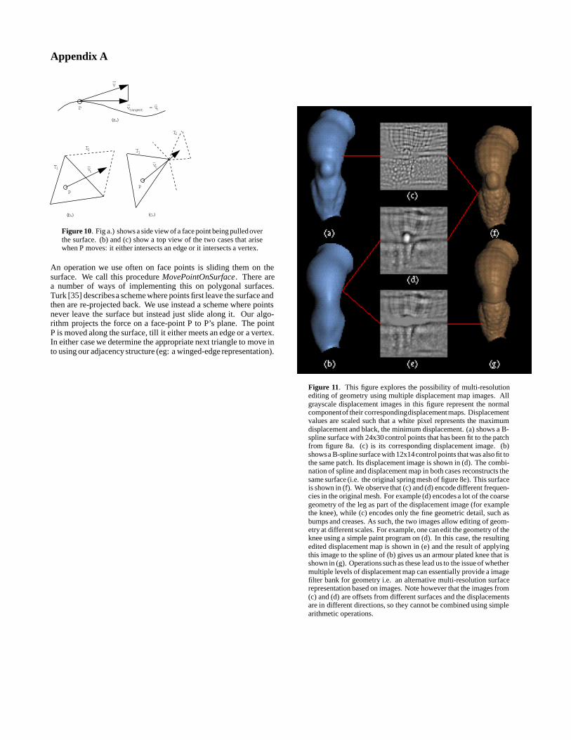
Figure 10. Fig a.) shows a side view of a face point being pulledoverthe surface. (b) and (c) show a top view of the two cases that arisewhen P moves: it either intersects an edge or it intersects a vertex.

An operation we use often on face points is sliding them on thesurface. We call this procedure MovePointOnSurface. There area number of ways of implementing this on polygonal surfaces.Turk [35] describesa scheme where points first leave the surface andthen are re-projected back. We use instead a scheme where pointsnever leave the surface but instead just slide along it. Our algo-rithm projects the force on a face-point P to P’s plane. The pointP is moved along the surface, till it either meets an edge or a vertex.In either case we determine the appropriate next triangle to move into using our adjacency structure (eg: a winged-edge representation).

Figure 11. This figure explores the possibility of multi-resolutionediting of geometry using multiple displacement map images. Allgrayscale displacement images in this figure represent the normalcomponentof their correspondingdisplacementmaps. Displacementvalues are scaled such that a white pixel represents the maximumdisplacement and black, the minimum displacement. (a) shows a B-spline surface with 24x30 control points that has been fit to the patchfrom figure 8a. (c) is its corresponding displacement image. (b)showsa B-spline surface with 12x14control points that was also fit tothe same patch. Its displacement image is shown in (d). The combi-nation of spline and displacement map in both cases reconstructs thesame surface (i.e. the original spring mesh of figure 8e). This surfaceis shown in (f). We observe that (c) and (d) encodedifferent frequen-cies in the original mesh. For example (d) encodes a lot of the coarsegeometry of the leg as part of the displacement image (for examplethe knee), while (c) encodes only the fine geometric detail, such asbumps and creases. As such, the two images allow editing of geom-etry at different scales. For example, one can edit the geometry of theknee using a simple paint program on (d). In this case, the resultingedited displacement map is shown in (e) and the result of applyingthis image to the spline of (b) gives us an armour plated knee that isshown in (g). Operations such as these lead us to the issue of whethermultiple levels of displacement map can essentially provide a imagefilter bank for geometry i.e. an alternative multi-resolution surfacerepresentation based on images. Note however that the images from(c) and (d) are offsets from different surfaces and the displacementsare in different directions, so they cannot be combined using simplearithmetic operations.

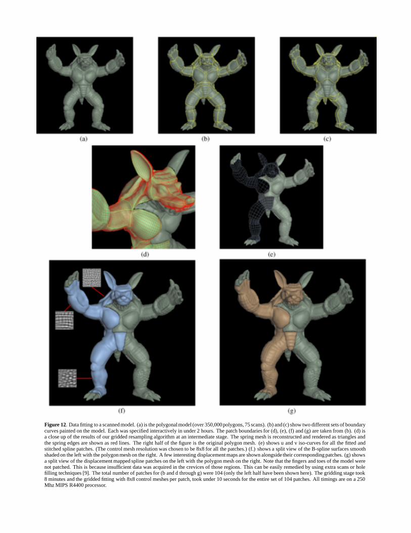
Figure 12. Data fitting to a scanned model. (a) is the polygonalmodel (over 350,000polygons, 75 scans). (b) and (c) show two different sets of boundarycurves painted on the model. Each was specified interactively in under 2 hours. The patch boundaries for (d), (e), (f) and (g) are taken from (b). (d) isa close up of the results of our gridded resampling algorithm at an intermediate stage. The spring mesh is reconstructed and rendered as triangles andthe spring edges are shown as red lines. The right half of the figure is the original polygon mesh. (e) shows u and v iso-curves for all the fitted andstitched spline patches. (The control mesh resolution was chosen to be 8x8 for all the patches.) (f.) shows a split view of the B-spline surfaces smoothshaded on the left with the polygon mesh on the right. A few interesting displacement maps are shown alongside their corresponding patches. (g) showsa split view of the displacement mapped spline patches on the left with the polygon mesh on the right. Note that the fingers and toes of the model werenot patched. This is because insufficient data was acquired in the crevices of those regions. This can be easily remedied by using extra scans or holefilling techniques [9]. The total number of patches for (b and d through g) were 104 (only the left half have been shown here). The gridding stage took8 minutes and the gridded fitting with 8x8 control meshes per patch, took under 10 seconds for the entire set of 104 patches. All timings are on a 250Mhz MIPS R4400 processor.

Figure 13. Games one can play with displacement maps: (a) shows a patch from the back of the model in 12a. The patch has over 25,000 vertices. Weobtained a spline fit (in 30 seconds) with a 15x20 control mesh, shown in (b) and a corresponding vector displacement map. The normal component ofthe vector displacement map, is displayed as a grayscale image in (c). (d) and (e) show the correspondingdisplacement and bump mapped spline surface.The differences between (d) and (e) are evident at the silhouette edges. The second row of images show a selection of image processing games on thedisplacement map. (f) shows jpeg compression of the displacement image to a factor of 10 and (g) shows compression to a factor of 20. (h) represents ascaling of the displacement image, to enhance bumps. (i) demonstrates a compositing operation, where an image with some words was alpha compositedwith the displacement map. The result is an embossed effect for the lettering. Finally, the third row of images (j - l) show transferring of displacementmaps between different objects. (j) is a relatively small polygonal model of a wolf’s head (under 60,000 polygons). It was fit with 54 spline patches inunder 4 minutes. The splined model is shown in (k). (l) shows a close up view of a partially splined result, where we have mapped the displacementmap from (c) onto each of 4 spline patches around the eyes of the model.