robert de mello koch - kavli ipmu-カブリ数物連携 ... · holography for heavy operators...
TRANSCRIPT
Holography for Heavy Operators
Robert de Mello Koch
Mandlestam Institute for Theoretical PhysicsUniversity of the Witwatersrand
August 4, 2016

The talk is based on work (arXiv:1608.00399) withDavid Gossman (MSc), Lwazi Nkumane (PhD) andLaila Tribelhorn (PhD).

Large N limits of matrix models are relevant forstrong coupling limits of non-Abelian gauge theoriesand for AdS/CFT.
Difficult problem, but has been solved for the singletsector of single matrix models.
Problem reduces to eigenvalue dynamics: HUGEreduction in degrees of freedom; non-interactingfermion dynamics; has found clear and convincingapplication in the 1/2 BPS LLM sector.(Brezin, Izykson, Parisi, Zuber; Ginibre; Corley, Jevicki, Ramgoolam;Berenestein; Lin, Lunin, Maldacena;...)

In this talk we ask if there is a similar eigenvaluedescription for a two matrix model and if this hassome AdS/CFT interpretation?
Naive answer: NO! We need to integrate over tworandom matrices and we can’t simultaneouslydiagonalize them!
Perhaps there is a class of questions (generalizingthe “singlet sector” of one matrix model) that canbe approached using eigenvalue dynamics?

Single Complex Matrix Model:
Use the Schur decomposition Z = U†D U with U aunitary matrix and D an upper triangular matrix, toexplicitly change variables. A standard argumentthen maps eigenvalue dynamics to non-interactingfermion dynamics.(Brezin, Izykson, Parisi, Zuber; Ginibre)
We could also construct a basis of operators thatdiagonalize the (free) inner product ⇒ Schurpolynomials ⇒ non-interacting fermions
〈χR(Z )χS(Z †)〉 = fRδRS
ψFF ∝ χR(Z )∆(Z )e−12
∑i zi zi
(Corley, Jevicki, Ramgoolam; Berenestein)

Single Complex Matrix Model
Each row of the Schur polynomial can be identifiedwith fermion ↔ an eigenvalue.
The number of boxes in each row tells us how mucheach fermion was excited.
If we were to study a two matrix model, with manyZ s and few Y s the rough outline of the abovepicture should still be visible.

Two Matrix Model: Restricted Schurs
For two matrices (Z ,Y ) we can diagonalize the freefield inner product with restricted Schur polynomials
〈χR,(r ,s)ab(Z ,Y )χT ,(t,u)cd(Z †,Y †)〉
= fRhooksR
hooksrhookssδRTδrtδsuδacδbd
(Bhattacharrya,Collins,dMK;Collins,dMK,Stephanou)
Operator built using n Z s and m Y s. We haver ` n, s ` m, R ` n + m. The restricted Schurpolynomials don’t diagonalize the dilatationoperator.

Two Matrix Model: Gauss Graph Operators
Using the restricted Schur polynomials as abasis, we can diagonalize the dilatationoperator in a limit in which R has order 1long rows and m n.
Operators are labeled by graphs - one nodefor each row. Directed edges connect nodes -one Y for each edge.(da Commarmond, dMK, Jefferies; dMK, Dessein, Giataganas, Mathwin;dMK, Ramgoolam)

Figure: Each node is a fermion = a giant graviton andthe edges stretching between nodes are open strings(each edge is a Y ) attached to the giant gravitonbranes

Non-interacting fermion description ⇒ consider onlyoperators labeled by Gauss graphs with no edgesstretching between nodes.
These are the BPS operators.
Figure: Non-interacting fermions are BPS operators

Non-interacting fermion description ⇒ onlyGauss graphs for BPS operators .
⇒ if there is a non-interacting fermiondescription at all, it will only describe BPSoperators.
These are associated to sugra solutions ofstring theory: only one-particle statessaturating the BPS bound in gravity areassociated to massless particles and lie in thesupergravity multiplet.

Eigenvalue dynamics as a dual tosupergravity has been advocated (usingdifferent reasoning) also by Berenstein; (see:0507203, 0605220, 0801.2739, 0805.4658, 1001.4509,
1404.7052). These works use a combination ofnumerical methods and physical arguments.
We obtain exact analytic statements abouteigenvalue dynamics, from multi-matrixquantum mechanics. The results agree withBerenstein.

From direct change of variables:
〈· · · 〉 =
∫[dZdZ †]e−TrZZ
† · · ·
=
∫ N∏i=1
dzidzie−∑
k zz zk∆(z)∆(z) · · ·
=
∫ N∏i=1
dzidzi |ψgs(z, z)|2 · · ·

ψgs(z, z) = ∆(z)e−12
∑k zz zk
∆(z) =
∣∣∣∣∣∣1 1 · · · 1z1 z2 · · · zN... ... ... ... ... ...
zN−11 zN−1
2 · · · zN−1N
∣∣∣∣∣∣We replaced dZ →
∏Ni=1 dzi ∆(z). Four
important observations:
I identical particles (Z → UZU†)I correct dimension (if [Z ] = L, need
[ψgs] = LN(N−1))I correct scaling under Z → e iθZI evenly spaced dimensions ⇒ oscillator
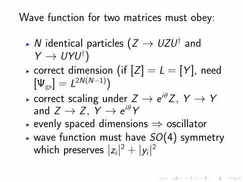
Wave function for two matrices must obey:
I N identical particles (Z → UZU† andY → UYU†)
I correct dimension (if [Z ] = L = [Y ], need[Ψgs] = L2N(N−1))
I correct scaling under Z → e iθZ , Y → Yand Z → Z , Y → e iθY
I evenly spaced dimensions ⇒ oscillatorI wave function must have SO(4) symmetry
which preserves |zi |2 + |yi |2

Guess for the wave function satisfying theseproperties:
Ψ(z, y) = ∆(z, y)e−12
∑k zk zk−
12
∑k yk yk
∆(z, y) =
∣∣∣∣∣∣∣∣∣∣yN−1
1 yN−12 · · · yN−1
N
z1yN−21 z2y
N−22 · · · zNy
N−2N... ... ... ... ... ...
zN−21 y1 zN−1
2 y2 · · · zN−1N yN
zN−11 zN−1
2 · · · zN−1N
∣∣∣∣∣∣∣∣∣∣

Matrix model computation:
〈Tr(Z J)Tr(Z †J)〉 =1
J + 1
[(J + N)!
(N − 1)!− N!
(N − J − 1)!
]if J < N and
〈Tr(Z J)Tr(Z †J)〉 =1
J + 1
(J + N)!
(N − 1)!if J ≥ N
Eigenvalue computation:∫ N∏i=1
dzidzidyidyi |Ψ(zi , yi )|2∑i
zJi∑j
zJj =1
J + 1
(J + N)!
(N − 1)!
⇒ we correctly reproduce (to all orders in 1/N) all singletraces of dimension N or greater.

We know that we will reproduce both Tr(Z J), Tr(Y J) forJ ≥ N .
There are trace relations implying
Tr(Z J) =∑i ,j ,...,k
cij ...kTr(Zi )Tr(Z j) · · ·Tr(Z k)
i , j , ..., k ≤ N and i + j + · · ·+ k = J so that we also start toreproduce sums of products of traces of less than N fields.
We can build BPS operators using both Y and Z fields -symmetrized traces. Are these correlators correctlyreproduced?
OJ,K =J!
(J + K )!Tr
(Y
∂
∂Z
)K
Tr(Z J+K )↔∑i
zJi yKi

Matrix model computation:
〈OJ,KO†J,K 〉 =J!K !
(J + K + 1)!
[(J + K + N)!
(N − 1)!− N!
(N − J − K − 1)!
]if J + K < N and
〈OJ,KO†J,K 〉 =J!K !
(J + K + 1)!
(J + K + N)!
(N − 1)!if J+K ≥ N
Eigenvalue computation:∫ N∏i=1
dzidzidyidyi |Ψ(zi , yi )|2∑i
zJi yKi
∑j
zJj yKj
=J!K !
(J + K + 1)!
(J + K + N)!
(N − 1)!
⇒ we again correctly reproduce (to all orders in 1/N) allsingle traces of a dimension N or greater.

Multitrace correlators are also reproduced exactly, as long asthey have a dimension J + K ≥ N
〈OJ1,K1OJ2,K2
· · ·OJn,KnO†J,K 〉
=J!K !
(J + K + 1)!
(J + K + N)!
(N − 1)!δJ1+···+Jn,JδK1+···+Kn,K
=
∫ N∏i=1
dzidzidyidyi |Ψ(zi , yi )|2∑i1
zJ1i1 yK1
i1· · ·∑in
zJnin yKn
in
×∑j
zJj yKj

Operator with a dimension of order N2: Young diagram Rwith N rows and M columns
χR(Z ) = (detZ )M = zM1 zM2 · · · zMN
χR(Z †) = (detZ †)M = zM1 zM2 · · · zMNThe two point correlator of this Schur polynomial is
〈χRχ†R〉 =
∫ N∏i=1
dzidzidyidyi |Ψ|2|z1|2M |z2|2M · · · |zN |2M
=
N∏i=1
(i − 1 + M)!
(i − 1)!
which is again the exact answer for this correlator. Not allSchur polynomials are correctly reproduced!

Local supersymmetric geometries with SO(4)× U(1)isometries have the form
ds210 = −h−2(dt + ω)2 + h2
[2
Z + 12
∂a∂bKdzadzb + dy 2
]+y (eGdΩ2
3 + e−Gdψ2)
y is the product of warp factors for S3 and S1 ⇒ mustimpose boundary conditions at y = 0 hypersurface to avoidsingularities: when S3 contracts to zero, we need Z = −1
2 and
when ψ-circle collapses we need Z = 12 .
(Donos; Lunin; Chen, Cremonini, Donos, Lin, Lin, Liu, Vaman, Wen)
There is a surface separating these two regions, and hence,defining the supergravity solution. Is this surface visible in theeigenvalue dynamics?

At large N we expect a definite eigenvalue distribution. Theseeigenvalues will trace out a surface specified by where thesingle fermion probability peaks
ρ(z1, z1, y1, y1) =
∫ N∏i=2
dzidzidyidyi |Ψ(z1, · · · , yN)|2 (1)
Denote the points lying on this surface by zMM , yMM .For the AdS5×S5 solution, the supergravity boundarycondition is
|z1|2 + |z2|2 = N − 1 (2)
The surfaces (1) and (2) are mapped into each other byidentifying z1 = zMM , z2 = yMM .

For an LLM annulus geometry (R has N rows and M columns)
Ψ(z , y ) = ∆(z , y )χR(Z )e−12
∑k zz zk−
12
∑k yz yk
determines ρ(z1, z1, y1, y1).
The supergravity boundary condition is
|z2|2 =M + N − 1− z1z1
z1z1 −M + 1
The map between the two surfaces is z2 = yMM√|zMM |2−M+1
,
z1 = zMM .
⇒ eigenvalues again condense on the surface that defines thewall between the two boundary conditions, agreeing with aproposal by Berenstein

Conclusions and questions:
I There is a sector of the two matrix modeldescribed (exactly) by eigenvalue dynamics. Inthe dual gravity these states are supergravitystates corresponding to classical geometries.
I The supergravity boundary conditions appear tomatch the large N eigenvalue description.
I How could one derive these results? How couldone argue for the relevance/applicability ofeigenvalue dynamics?
I Can this be extended to more matrices?
I Can the eigenvalue dynamics be perturbed byoff diagonal elements to start including stringydegrees of freedom?

Thanks for your attention!