Rob FowlerRenaissance Computing Institute/UNC

USQCD Software Committee MeetingFermiLab

Nov 7, 2008

SciDAC PERI and USQCD Interaction: Performance Analysis and

Performance Tools for Multi-Core Systems

Caveats

• This talk got moved up a day and my flight was delayed, so slide prep. time got truncated, especially the editing part.

• This is an overview of activities, current and near future.

• January review talk will focus more narrowly.– We need to coordinate our presentations

to share the same narrative.

Roadmap for Talk

• Recent and Current Activities.– PERI Performance Database– On-node performance analysis and tools.– Multi-core tools, analysis, …

• Near Future– PERI scalable tools on DOE systems.– NSF Blue Waters system.

Databases and workflows.

• RENCI is running a PERI performance database server.– Being used for tuning campaigns,

regression testing.– Demand or interest within USQCD?

• Several projects involving ensembles of workflows of ensembles.– Leverage within USQCD?

HPCToolkit Overview(Rice U, not IBM)

• Uses Event-Based Sampling.– Connect a counter to an “event” through

multiplexors and some gates.– while (profile_enabled) { <initialize counter to negative number> <on counter overflow increment a histogram

bucket for current state (PC, stack, …)> }

• Uses debugging symbols to map event data from heavily optimized object code back to source constructs in context.

• Computes derived metrics (optional).• Displays using a portable browser.

MILC QCD code in Con Pentium DFlat, source view(One node of a parallel run.)

LQCD Code As a Driver for Performance Tool Development

• HPCToolkit analyzes optimized binaries to produce an object source map.

• Chroma is a “modern” C++ code– Extensive use of templates and inlined methods– Template meta-programming.

• UNC and Rice used Chroma to drive development of analysis methods for such codes (N. Tallent’s MS Thesis.)

• Other DOE codes are starting to benefit.– MADNESS chemistry code– GenASIS (Successor to Chimera core-collapse supernova code)/

• Remaining Challenge in the LQCD world– Analyze hand-coded SSE.

• asm directives should preserve line number info, but inhibit further optimization.

• Using SSE intrinsics allows back-end instruction scheduling, but every line in the loop/block was included from somewhere else. Without line numbers associated with local code, there’s too little info r.e. the original position at which the instruction was included.

Flat, “source-attributed object code” viewof the “hottest” path.

Chroma

Chroma

Flat, “source-attributed object code” viewof the “second hottest” path.

Chroma

Call stack profile

The Multicore Imperative:threat or menace?

• Moore’s law put more stuff on a chip.– For single-threaded processors, add

instruction level parallelism.• Single-thread performance has hit the walls:

complexity, power, …– “Solution”: implement explicit on-chip

concurrency: multi-threading, multi-core.– Moore’s law for memory has increased

capacity with modest performance increases.• Issues: dealing with concurrency

– Find (the right) concurrency in application.– Feed that concurrency (memory, IO)– Avoid or mitigate bottlenecks.

Resource-Centric Tools for Multicore

• Utilization and serialization at shared resources will dominate performance.– Hardware: Memory hierarchy, channels.– Software: Synchronization, scheduling.

• Tools need to focus on these issues.• It will be (too) easy to over-provision a chip

with cores relative to all else.• Memory effects are obvious 1st target

– Contention for shared cache: big footprints– Bus/memory utilization.– DRAM page contention: too many streams

• Reflection: make data available for introspective adaptation.

Cores vs Nest Issues for HPM Software

• Performance sensors in every block.– Nest counters extend the

processor model.• Current models:

Process/thread centric monitoring

Virtual counters follow threads. Expensive, tricky.

Node wide, but now (core+PID centric)

– Inadequate monitoring of core-nest-core interaction.

– No monitoring of fine grain thread-thread interactions (on-core resource contention).

• No monitoring of “concurrency resources”.

Nest Cores

Aside: IBMers call it the “nest”. Intel uses “UnCore”

Another view: HPM on a Multicore Chip.

FPU

L2

L1

CTRS

Core 0

FPU

L2

L1

CTRS

Core 1

FPU

L2

L1

CTRS

Core 2

FPU

L2

L1

CTRS

Core 3

NestL3

DDR-A DDR-B DDR-C

Mem-CTL

HT-1 HT-1 HT-1 NIC

= Sensor = Counter

HPM on a Multicore Chip.Who can measure what.

FPU

L2

L1

CTRS

Core 0

FPU

L2

L1

CTRS

Core 1

FPU

L2

L1

CTRS

Core 2

FPU

L2

L1

CTRS

Core 3

NestL3

DDR-A DDR-B DDR-C

Mem-CTL

HT-1 HT-1 HT-1 NIC

= Sensor = Counter

Counters within a core can measure events in that core, or in the nest.

RCRTool Strategy:

FPU

L2

L1

CTRS

Core 0

FPU

L2

L1

CTRS

Core 1

NestL3

DDR-A DDR-B DDR-C

Mem-CTL

HT-1 HT-1 HT-1 NIC

= Sensor = Counter

FPU

L2

L1

CTRS

Core 2

FPU

L2

L1

CTRS

Core 3

One core (0) measures nest events. The others monitor core events.Core 0 processes the event logs of all cores. Runs on-node analysis.MAESTRO: All other “jitter” producing OS activity confined to core 0.

HPM driver EBS events IBS events

HPM driver EBS events IBS events

RCRTool Architecture.Similar to, but extends DCPI, oprofile, pfmon, …

Tag

PC F1 F2

Kernel space log

HPM driver EBS events IBS events

HPM driver: Core 0 EBS events IBS events

Context switches

Locks, queues, etc.

Analysis Demon

Histograms, conflict graphs, on-line summaries and off-line reports.

Power monitors

HW Events SW Events

Multicore Performance issues:for LQCD and in general

Hybrid programming models for Dslash• Run Balint’s test code for Dslash on 8x8x4x4 local problem size on 1 and 2 chips in a Dell T605

(Barcelona ) system . Try three strategies.– MPI everywhere – vs MPI + OpenMP – vs MPI + QMT. (Balint’s test code.)

• OpenMP version less than 1/5 the performance of the QMT version (2.8 GFlops vs 15.8 GFlops).– Profiling reveals that showed that each core entered the HALTED state for significant

portions of the execution.– GCC OpenMP (version 2.5) uses blocking synchronization that halts idle cores. Relative

performance improves when the parallel regions are much longer. Possible optimization: consolidate parallel regions. (OpenMP version 3.0 has environment variable to control this behavior)

• Profiling revealed 2.1 GB/sec average memory traffic in the original QMT version.

– We removed software prefetching and non-temporal operations. (HW prefetching is still about 40% of traffic.)

– Minor change in memory utilization but QMT DSlash sped up by ~4% (from 15.8 GFlops to 16.5 GFlops)

– Remaining memory traffic is in the synchronization spin loop. (See next slide.)

– Scaling for this problem size is (1 thread =3.8 Gflops, 4 threads = 11.2 GFlops and 8 threads = 16.5 GFlops)

– Profiling with RCRTool prototype (to be discussed) reveals time and cache misses was incurred in barrier synchronization.

– With 4 threads – 4.5% of time spent at barriers. Thread zero always arrives first.– With 8 threads – 3x more cycles spent at barrier (compared to 4 threads) . Cost incurred

in the child threads because they always arrive arrive first!– Problem size clearly too small for 8-threads on the node.

OpenMP Streams on k cores.Build OpenMP version of Streams using std.

optimization levels (gcc -O3). Run on systems with DDR2 667 memory. (triad)

Threads 1 2 4

Xeon 51502chips x 2 cores

3371 5267 5409

Athlon 64,3 GHz1chip x 2 cores

3428 3465 {3446}

Opteron, 2.6GHz2 chips x 2 cores

3265 6165 7442

Conclusion – If Streams is a good predictor of your performance, then extra cores won’t help a lot unless you have extra memory controllers and banks.

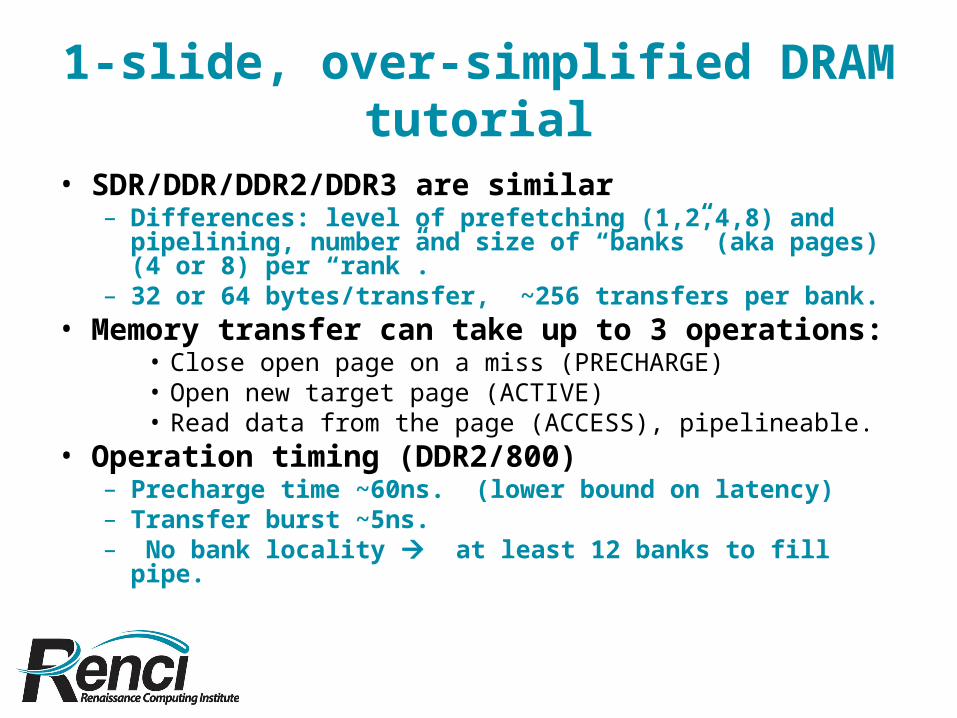
1-slide, over-simplified DRAM tutorial

• SDR/DDR/DDR2/DDR3 are similar– Differences: level of prefetching (1,2,4,8) and

pipelining, number and size of “banks” (aka pages) (4 or 8) per “rank”.

– 32 or 64 bytes/transfer, ~256 transfers per bank.• Memory transfer can take up to 3

operations:• Close open page on a miss (PRECHARGE)• Open new target page (ACTIVE)• Read data from the page (ACCESS), pipelineable.

• Operation timing (DDR2/800)– Precharge time ~60ns. (lower bound on latency)– Transfer burst ~5ns.– No bank locality at least 12 banks to fill pipe.

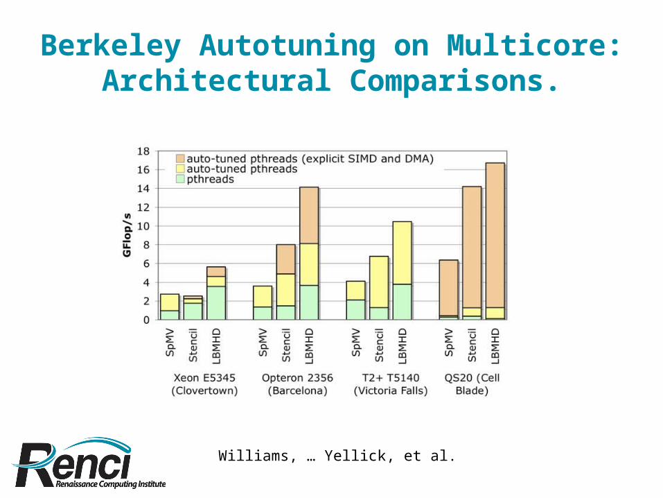
Berkeley Autotuning on Multicore:Architectural Comparisons.

Williams, … Yellick, et al.

Berkeley AMD vs Intel Comparison

Williams, … Yellick, et al.

Bandwidth, Latency, and Concurrency

• Littles Law (1961): L = λS, where– L = Mean queue length (jobs in system)– λ = Mean arrival rate– S = Mean residence time

• Memory-centric formulation: Concurrency = Latency x Bandwidth

• Observation– Latency determined by technology (& load)– Concurrency

• Architecture determines capacity constraints.• Application (& compiler) determines demand.

Achieved bandwidth is the dependent variable.

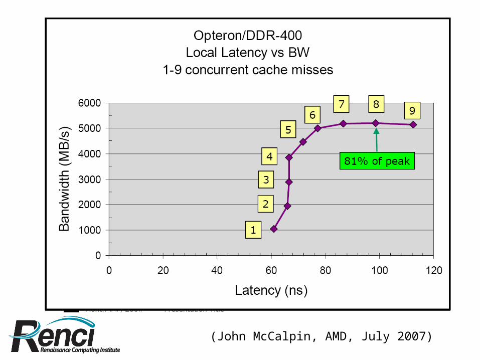
(John McCalpin, AMD, July 2007)

Bandwidth measured with Stream.

Compiled with GCC, so there’s considerable single thread bandwidth left on the table vs PathScale or hand-coded.

Concurrency and Bandwidth Experiments.

• Create multiple, pinned threads.• Each thread executes k semi-

randomized “pointer chasing” loops.– “semi-” means randomized enough to

confound the compiler and HW prefetch, but not so much that TLB misses dominate.

Low-Power Blade BW.

Dell PowerEdge M600• 2 x 1.9 GHz Barcelona•8 x 2G DDR667

X axis – number of concurrent outstanding cache misses.Y axis – effective bandwidth, assuming perfect spatial locality, i.e. use the whole block.

WS1: 4 x 512MB vs WS2: 8 x 512MB

Dell T605 2 x 2.1 GHz AMD Barcelona

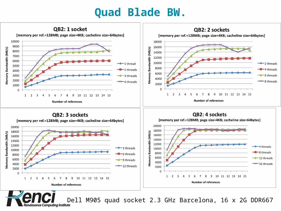
Quad Blade BW.

Dell M905 quad socket 2.3 GHz Barcelona, 16 x 2G DDR667

SciDAC PERI Scalable Tools.

• DOE funding targets DOE leadership class systems and applications.– Focus explicitly on problems that arises only

at scale: balance, resource limits, …– Tools work on Cray XTs at Cray. Waiting for

OS upgrades on production systems.

• Will be ported to NSF Blue Waters.– Two likely collaborations: MILC benchmark

PACT, SciDAC code team.

• Target apps: AMR, data dependent variation.– Useful for Lattice applications?

The need for scalable tools.(Todd Gamblin’s dissertation work.)

• Fastest machines are increasingly concurrent– Exponential growth in

concurrency– BlueGene/L now has

212,992 processors– Million core systems

soon.

• Need tools that can collect and analyze data from this many cores

Concurrency levels in the Top 100

Concurrency levels in the Top 100

http://www.top500.org

Too little disk space for all the

data

Too little disk space for all the

data

Challenges for Performance Tools• Problem 1: Measurement

– Each process is potentially monitored

– Data volume scales linearly with process count

• Single application trace on BG/L-sized system could consume terabytes– I/O systems aren’t scaling

to cope with this– Perturbation from

collecting this data would be enormous

Too little I/O bandwidth to

avoid perturbation

Too little I/O bandwidth to

avoid perturbation

Challenges for Performance Tools• Problem 2: Analysis

– Even if data could be stored to disks offline, this would only delay the problem

• Performance characterization must be manageable by humans– Implies a concise description– Eliminate redundancy

• e.g. in SPMD codes, most processes are similar

• Traditional scripts and data mining techniques won’t cut it– Need processing power in proportion to

the data– Need to perform the analysis online, in

situ

Scalable Load-Balance Measurement

• Measuring load balance at scale is difficult– Applications can use data-dependent,

adaptive algorithms– Load may be distributed dynamically

• Application developers need to know:1.Where in the code the problem occurs2.On which processors the load is

imbalanced3.When during execution imbalance occurs

Load-balance Data Compression

• We’d like a good approximation of system-wide data, so we can visualize the load

• Our approach:1. Develop a model to describe looping

behavior in imbalanced applications2. Modify local instrumentation to record

model data.3. Use lossy, low-error wavelet

compression to gather the data.

Progress/Effort Model• All interesting metrics are rates.

– Ratios of events to other events or to time: IPC, miss rates, …– Amount of work, cost, “bad things” that happen per unit of

application: cost per iteration, iterations per time step, …

• We classify loops in SPMD codes– We’re limiting our analysis to SPMD for now– We rely on SPMD regularity for compression to work well

• 2 kinds of loops:– Progress Loops

• Typically the outer loops in SPMD applications• Fixed number of iterations (possibly known)

– Effort Loops• Variable-time inner loops in SPMD applications• Nested within progress loops• Represent variable work that needs to be done

– Adaptive/convergent solvers– Slow nodes, outliers, etc.

Wavelet Analysis

• We use wavelets for scalable data compression

• Key properties:– Compact– Hierarchical– Locality-preserving– When filtered, have the right kind of non-

linearities.

• Technique has gained traction in signal processing, imaging, sensor networks– Has not yet gained much traction in performance

analysis

Initial InputLevel 0

Initial InputLevel 0

Wavelet AnalysisFundamentals

• 1D Discrete wavelet transform takes:

– samples in the spatial domain• transforms them to:

– coefficients of special polynomial basis functions in

– Space of all coefficients is the wavelet domain

– Basis functions are wavelet functions

• Transform can be recursively applied

– Depth of recursion is the level of the transform

– Half as much data at each level

• 2D, 3D, nD transforms are simply composite of 1D transforms along each dimension

Wavelet TransformWavelet Transform

lthlevellthlevel

Detail coefficients

Avg. Coefficients

l+1st

level

(Low frequency) (High frequency)

Wavelet Analysis

• Compactness– Approximations for most functions require very few terms in the

wavelet domain– Volume of significant information in wavelet domain much less

than in spatial domain

• Applications in sensor networks:– Compass project at Rice uses distributed wavelet transforms to

reduce data volume before transmitting– Transmitting wavelet coefficients requires less power than

transmitting raw data

• Applications in image compression:– Wavelets used in state-of-the-art compression techniques– High Signal to Noise Ratio

• Key property:– Wavelets preserve “features”, e.g., outliers that appear as high-

amplitude, high-frequency components of the signal.

Parallel Compression• Load data is a

distributed 3D matrix– N progress steps xR

effort regions per process

– 3rd dimension is process id

• We compress the effort for each region separately– Parallel 2D wavelet

transform over progress and processes

– Yields R compressed effort maps in the end

Parallel Compression• Wavelet transform

requires an initial aggregation step– We aggregate and transform

on all Rregions simultaneously

– Ensures all processors are used.

• Transform uses CDF 9/7 wavelets– Same as JPEG-2000

• Transformed data is thresholded and compressed– Results here are for run-

length + huffman coded– New results forthcoming for

EZW coding

Results: I/O Load• Chart shows time to

record data, with and without compression– Compression time is fairly

constant, and data volume never stresses I/O system

• Suitable for online monitoring

– Writing out uncompressed data takes linear time at scale

• 2 applications:– Raptor AMR– ParaDiS Crystal Dynamics

Results: Compression

• Compression results for Raptor shown– Each bar represents distribution of values over all the

effort regions compressed– Black bar is median, bar envelops 2nd and 3rd quartiles

• 244:1 compression ratio for a 1024-process run– Median Normalized RMS error ranges from 1.6% at lowest

to 7.8% at largest

Results: Qualitative

• Exact data and reconstructed data for phases of ParaDiS’s execution– Exact shown at top, reconstruction at bottom.

Force Computation

Force Computation

CollisionsCollisions RemeshRemeshCheckpointCheckpoint