Roadblock to Innovation: The Role of Patent Litigation in Corporate

R&D

Filippo Mezzanotti∗

First Draft: January 2015This Draft: December 7, 2017

Abstract

Using a difference-in-difference design around the Supreme Court decision “eBay vs. MercExchange,” I

examine how patent enforcement affects corporate R&D. To identify the effects of the decision, I compare

innovative activity across firms differentially exposed to patent litigation before the ruling. Across several

measures, I find that the decision led to a general increase in innovation. This result confirms that the

changes in enforcement induced by the ruling reduced some of the distortions caused by patent litigation.

Exploring the channels, I show that patent litigation negatively affects investment because it lowers the

returns from R&D and exacerbates its financing constraints.

JEL CODES: G30, G38, K11, O34

∗Kellogg School of Management, Northwestern University. I thank my advisors Josh Lerner, David Scharfstein, Andrei Shleifer,and Jeremy Stein, for their guidance and encouragement. I also thank Lauren Cohen, Jiashuo Feng, Samuel G. Hanson, VictoriaIvashina, Xavier Jaravel, Louis Kaplow, James Lee, Simone Lenzu, Christopher Malloy, Diana Moreira, Gianpaolo Parise, AndreaPassalacqua, Tom Powers, Giovanni Reggiani, Jonathan Rhinesmith, Tim Simcoe, Stanislav Sokolinski, Adi Sunderam, HarisTabakovic, Edoardo Teso, Rosemarie Ziedonis, John Zhou and the seminar participants at Boston University Technology Initiativeconference, Northwestern Law, EFA, Harvard University, Columbia University, Yale, Cornell, University of Rochester, FED Board,Texas A&M, Bocconi, and Cornerstone for helpful comments. In particular, I thank two discussants, Luke Stein and Pere Arque-Castells, for useful comments. I thank Harvard University, Harvard Business School, and Kellogg School of Management forfinancial support. All errors are my own. Email: filippo.mezzanotti@kellogg.northwestern.edu.

1 Introduction

The main goal of the patent system is to protect intellectual property and thus to spur innovation and growth.

Whether this goal is achieved depends on how patents are defined and protected, which itself depends on how

the legal system resolves intellectual-property disputes. Indeed, the courts appear to have played an increasingly

important role in the patent system. Over the last thirty years, lawsuits involving patents more than tripled

(Figure 1) and their estimated cost surpassed $300 billion (Bessen et al., 2015).1 Furthermore, a large share of

this increase can be explained by a surge in lawsuits involving patent-assertion entities, also known colloquially

as “patent trolls” (Cohen et al., 2014). This rise in litigation may reduce the incentives of firms to invest in

R&D, and therefore curb innovation and growth (Bessen and Meurer, 2008b; Boldrin and Levine, 2002; Jaffe

and Lerner, 2011).

In this paper, I show that changes in patent enforcement – by affecting the risk of litigation – can have sizable

effects on corporate R&D. To examine this issue, I develop a new research design that exploits a landmark legal

decision, the 2006 Supreme Court decision “eBay vs. MercExchange.” The ruling increased the flexibility in

the way courts remedy patent violations, by ending the practice of granting a permanent injunction almost

automatically after a violation. This shock is a fundamental change in patent enforcement because injunction

represents one of the major risks for firms accused of violating a patent. In fact, an injunctive order will force a

company to shut down any operation related to the violated technology, regardless of the nature and magnitude

of the infringement. In line with some of the law narrative on the case, my results confirm that the new rules

were successful in reducing part of the overhang that patent litigation imposes on innovative firms.

Before the ruling, many experts criticized the presence of automatic injunction, arguing that this norm

was giving too much power to companies that were interested in profiting from patent litigation. To quote

the Supreme Court, the threat of injunction was frequently used “as a bargaining tool to charge exorbitant

fees to companies that seek to buy licenses to practice the patent” (Court, 2006). Indeed, previous research

has shown that the presence of a “near-mandatory” injunction should increase the extent to which companies

can be held up by a plaintiff (Lemley and Shapiro, 2006; Shapiro, 2010, 2016a). Furthermore, because of the

complementarity between technologies and the high degree of uncertainty characterizing the patent system

(Lemley and Shapiro, 2005), the threat of injunction can be very pervasive even when accusations are based on

frivolous claims or minor violations.

A prominent example that demonstrates the important role of injunction in patent litigation is the lawsuit

between Research in Motion (RIM), BlackBerry’s producer, and NTP in the early 2000s. After the court found

RIM guilty of infringing a few patents owned by NTP, RIM started to negotiate with NTP with the objective of

avoiding an injunction. In fact, even if the infringement covered only a small fraction of the portfolio of patents

used to run the Blackberry system, an injunction order would likely have led to a shutdown of the system, given1This estimate refers only to public firms sued by nonpracticing entities, and it is constructed using an event-study methodology.

1

the complementarity across technologies in the platform. Leveraging on its ability to obtain an injunction,

NTP was able to obtain a record settlement, which amounted to more than $610 million, more than half of

RIM revenues in the previous year. Interestingly, years later some of the claims contained in NTP patents were

deemed invalid, as RIM had argued initially. According to several experts, the presence of automatic injunction

played a fundamental role in the decision to settle early and the size of the transfer.2

In theory, this increase in court flexibility has an ambiguous effect on firm innovation activity. On the one

hand, the reduction of the hold-up problem in litigation may increase innovation by lowering the burden of

abusive patent lawsuits. In particular, removing automatic injunction reduces the risks faced by firms accused

of patent violation and therefore it should lower the amount of money that companies have to spend in terms of

settlements, licensing, and legal costs.3 In turn, this will affect the incentives and the financial ability of firms

working in R&D. On the other hand, a reduction in injunctions may also lower deterrence against violations

(e.g., Epstein, 2008) and more generally reduce innovation appropriability. The overall effect will depend on

the size of the ex-ante hold-up costs and on how the new rules will remove some of the distortions of automatic

injunction but still allow firms to be fairly compensated for their innovation.

I start by reviewing some of the recent empirical work that examines how the new rules affected the legal

activity.4 As expected, the new rules had a significant effect in reducing the likelihood of obtaining an injunction.

For instance, Chien and Lemley (2012) found that the likelihood of obtaining an injunction decreased by at least

25%.5 However, permanent injunction remains a tool available to firms, since it is still granted in a majority

of cases, in particular when this action appears to be the only way to remedy the violation. In this regard,

Seaman (2016) finds that the decline in injunction rates is mostly driven by cases where the two parties are not

competitors or when it involves a nonpracticing entity (PAE). Consistently with this result, I find that public

PAE experienced large negative returns around the time of the decision, with average cumulative returns of

about -10%. Therefore, this evidence suggests that the new rules did not bring about a reduction in protection

for incumbent innovative firms, but rather they gave courts the ability to avoid the issuance of an injunction

when more efficient remedies are available. While this narrative seems to be more consistent with a more

benevolent interpretation of the effects of the ruling, direct evidence is necessary to determine its real impact.

To provide this direct evidence, I estimate the causal impact of the decision using a difference-in-difference

design that exploits heterogeneity in the intensity of the treatment. In particular, I use variation in firm2In an interview for the National Law Journal (March 13, 2006, Volume 27, Issue 77), patent litigator David Clonts of Akin

Gump Strauss Hauer & Feld’s, states that “If BlackBerry knew it could successfully defend against an injunction and instead havea trial on money damages, the settlement value would have been a tenth of what it was.”

3This view was shared by many scholars and practitioners. According to the American Innovators Alliance, an associationrepresenting large high-tech companies like Microsoft, Micron, Oracle and Intel, because of high injunction risk, “money that couldgo to productive investments is instead diverted to legal fees and settlement payments,” leading to “... less innovation.” Thesentences are taken from the “amicus curiae” submitted for the Supreme Court case.

4Similar results are also confirmed in qualitative work, for instance\ e.g., Bessen and Meurer (2008a); Holte (2015); Shapiro(2010); Tang (2006); Venkatesan (2009).

5As discussed later in the paper, Gupta and Kesan (2015); Seaman (2016); Grumbles III et al. (2009) find results consistentwith those in Chien and Lemley (2012).

2

exposure to patent litigation in 2006 to identify companies that are more likely to be affected by the decision.

The intuition for this is simple: while the shock potentially touched every firm, companies that operate in areas

where patent litigation is more intense should be relatively more affected by the decision. In particular, my

measure of litigation exposure captures variation in the risk of litigation that exogenously affects a company

because it innovates in specific technology fields. Looking across more than four hundred technology classes

defined by the U.S. patent office, I identify the fields where each company operates. Moreover, I create a

measure of patent litigation intensity for each of these fields using litigation data from WestLaw (Thomson

Reuters). The final firm-level measure of exposure to patent litigation is simply a weighted average of litigation

intensity across all the technology classes, where the weights are the share of patents developed in each class

by the company.

As a first step, I implement this estimator by examining the patent application for a sample of almost

twenty thousand innovative firms. Firms that were more exposed to litigation before the decision increased

patenting more after the decision. These effects are not only statistically significant, but also economically

relevant. For example, examining two firms one standard deviation apart in exposure to litigation, I find that

the more exposed company increased patent applications 3% more than the less exposed one, which on average

corresponds to almost one extra patent in the two years after the shock. Similarly, the same firm was 2% more

likely to patent something, which is equivalent to a 5% jump in the probability of patenting in the sample. As

discussed in the paper, these results are not driven by differential trends across heterogeneously exposed firms,

and they are robust to control for firm-industry trends – measured by the main technology area of the firm

(Hall et al., 2001) – as well as other confounding factors.

However, this increase in patenting activity does not necessarily have to translate into an increase in inno-

vation. First, a simple count of patents cannot distinguish between increases in new innovative activity and a

change in the incentives to patent. Second, if the new rules really lower deterrence against new violations, the

increase in patenting may simply be reflecting more defensive activity (Hall and Ziedonis, 2001; Ziedonis, 2004).

To rule out these two alternative explanations, I provide two sets of tests.

First, I use patent data to measure changes in the quality or type of innovation that was undertaken. While

increasing patenting relatively more, firms more exposed to patent litigation did not lower the average quality

of their output. Instead, they became relatively more likely to develop a potential “breakthrough innovation”

(Kerr, 2010), defined as a patent that is at the top of the citation distribution within the same patent class and

year group. At the same time, contrary to the defensive hypothesis, I find that the share of defensive activity

increased relatively less for highly exposed firms. To start, I examine defensive activity by measuring patenting

that is of low quality but that cites an exceptionally dispersed set of different technologies. This measure builds

on the intuition that the value of a defensive patent does not depend on the quality of the idea, but rather

3

on its breadth in covering a technology space.6 However, as an alternative measure, I also find similar results

looking directly at business-method patents, which were an important target class of patents used in strategic

litigation during this time.

Second, I focus on a sub-sample of public firms that were active in innovation around the decision. Using the

same methodology as before, I find that the ruling also increased R&D intensity. When comparing two firms

that are one standard deviation apart in terms of exposure to patent litigation, I find that the more exposed

firm experienced a relative increase of 8% in R&D over assets.

Overall, firms more exposed to patent litigation appeared to have relatively outperformed other firms in

terms of both innovation output and input. Evidence on patent quality, patent type, and R&D investment

seems to be consistent with the interpretation that companies responded to the new rules by doing more

innovation activity. These results suggest that better patent enforcement can increase the certainty with which

intellectual property is protected and reduce the risks of hazardous litigation, thereby increasing the incentive

of firms to invest in R&D. As a final robustness to this mechanism, I also find that the positive effect on R&D

was more pronounced for firms that were less likely to be involved in litigation as a plaintiff.

Finally, I examine how an improvement in enforcement rules may affect the process of innovation. First, a

change in enforcement should affect firms’ activity by affecting the returns to innovation. If this channel were

economically sizable, after a change in enforcement we should expect on average a shift in innovation activity

towards projects that were riskier ex ante. To test this mechanism, I explore the within-firm propensity to

work in areas with a high risk of litigation to provide evidence in line with this idea. Consistent with the

previous findings, firms reshuffled their internal resources towards projects in higher litigation areas, at least at

the extensive margin.

Second, worse enforcement rules should also affect R&D by exacerbating the financing problems of innovation

(Brown et al., 2009; Hall and Lerner, 2010). In fact, companies operating in high-litigation environments should

be forced to devote a larger share of resources to monitoring and defensive activities (Cohen et al., 2014) and

spend more money on settlements or licensing.7 In the presence of financial frictions, the increase in costs

reduces the amount of resources available and therefore forces firms to cut down on investments. Consistent

with this implication, firms that were more likely to be financially constrained before the decision increased

R&D intensity more in its aftermath. These findings establish the important role played by financial constraints

in explaining the negative effects of patent litigation.8

6In fact, Abrams et al., 2013 find that patents with a high strategic value are actually of low quality.7Litigation claims “whether meritorious or not, (. . . ) could require expensive changes in our methods of doing business, or could

require to enter into costly royalty or licensing agreements” (eBay 2006 10-K).8A large literature in finance suggests that more and better innovation can increase firms’ valuation (Kogan et al., 2012). In line

with this research, I find that the decision had a positive effect on stock market returns. By looking at abnormal returns on theday that the decision was made public, I demonstrate that firms that are characterized by high exposure had larger returns, andthat this effect does not disappear over the following days. For instance, looking across the top quartile of treatment, I find thatvalue-weighted returns of the two groups are identical before the announcement, but that the more exposed group outperformedthe other group by 80 bps on the day of the announcement.

4

By showing that changes in patent enforcement can have sizable effects on corporate innovation, this paper

contributes to the literature that examines how property rights and legal institutions shape economic incentives

(Acharya et al., 2011; Claessens and Laeven, 2003; Demirgüç-Kunt and Maksimovic, 1998; King and Levine,

1993; La Porta et al., 1997; Lerner and Schoar, 2005).9 Previous research has demonstrated that secure property

rights favor a more efficient allocation of resources and foster growth, but in many cases good enforcement is as

important as good rules in determining economic outcomes (e.g. Djankov et al., 2003). The role of enforcement

is particularly important in intellectual property because the exact boundaries of patents are hard to define

(Lemley and Shapiro, 2005) and therefore lawsuits are frequent (Lanjouw and Lerner, 1998). This paper

highlights the role of enforcement in innovation and suggests that, similarly to other interventions (Acharya and

Subramanian, 2009; Mann, 2013), a fine-tuning of patent law can have substantial effects on fostering corporate

innovation.

Furthermore, this analysis also provides new evidence about the real costs of patent litigation, which is

central in today’s policy debate (White House 2013) and research (Hall and Harhoff, 2012). While the idea

that litigation could harm innovation is generally accepted, direct evidence that supports this claim is relatively

sparse. In this direction, Smeets (2014) shows that firms decrease R&D intensity after being litigated. My

results are consistent with his work and extend his idea by showing that high litigation may harm innovation

by affecting firms’ ex-ante incentives, independently of whether the firm was directly engaged in any activity.

Furthermore, my work provides new insights on the operation of nonpracticing entities and contributes to the

growing literature on this topic (Appel et al., 2016; Cohen et al., 2014; Feng and Jaravel, 2015; Kiebzak et al.,

2016; Tucker, 2014).

Lastly, this paper also adds to the body of empirical work that analyzes the role of intellectual property

rights in fostering innovation. Previous work suggests that intellectual property reduces follow-up innovation

(Galasso and Schankerman, 2015; Murray and Stern, 2007; Williams, 2015), and more generally the literature

provides very little evidence that stronger property rights translate into more innovation (Lerner, 2002, 2009;

Moser, 2005, 2013; Sakakibara and Branstetter, 2001). Relative to this area, this paper provides evidence that

is consistent with these results, by showing that restricting certain enforcement rights of patent holders may

have beneficial effects for innovation.10 This result is somehow not surprising within the context of the law and

economics literature, which has long debated about optimal enforcement rules. A strict property rule – like in

the case of mandatory injunction – works well when ownership rights are clear and easy to identify, as with

tangible assets (Calabresi and Melamed, 1972). If the boundaries of the assets are hard to define, like in the

case of patents (Lemley and Shapiro, 2005), a strict property rule may fail to provide the best incentives, and

it may be inferior to a hybrid system that provides more flexibility (Kaplow and Shavell, 1996). An implication9This topic is related to the finance literature focusing on the relationship between litigation and corporate policies (Arena and

Julio, 2014; Kim and Skinner, 2012; Haslem, 2005; Rogers and Van Buskirk, 2009).10During the argument, Justice Scalia said, “We’re talking about a property right here, and a property right is the exclusive right

to exclude others.”

5

is that patents are different from other assets, and therefore the design of their enforcement should take into

account these differences (Schwartzstein and Shleifer 2013).

The paper is organized as follows. In Section (2), I provide more background information about the Supreme

Court decision, also discussing its potential effects on corporate innovation. In Section (3), I present the data

used in the paper and discuss in detail how I construct my measure of exposure to patent litigation at the

firm level. In Section (5), I present the main results of my analysis. In Section (6), I discuss and test different

channels through which patent litigation can affect innovation. In Section (A.5.2), I look at the stock market

reaction around the decision. Lastly, Section (7) discusses policy implications and avenues for future research.

2 The “eBay vs. MercExchange” case

This section provides background information on the Supreme Court decision “eBay vs. MercExchange” and

discusses its possible effects on innovation. First, I analyze the importance of injunction on the pre-eBay world,

in particular with respect to litigation. Second, I discuss how the ruling could affect innovation, therefore setting

the foundation for the hypothesis and research design. Lastly, I provide some preliminary and novel evidence

of the importance of the ruling for patent enforcement.

2.1 The role of injunction and the 2006 decision

With the 2006 “eBay vs. MercExchange” decision, the Supreme Court revisited the norms regulating the

issuance of permanent injunction in cases involving intellectual property.11 Injunction is a legal remedy that

can be requested by a plaintiff after a violation. If granted by a court, an injunction forces the infringer to stop

using any technology covered by the contested patents, irrespective of the magnitude of the infringement. Before

2006, a plaintiff that was able to prove a violation had essentially the automatic right to obtain a permanent

injunction. In other words, the norm was that “a permanent injunction should be issued when infringement

was proven” (Court, 2006). Exceptions to this rule were quite uncommon and mostly due to reasons of public

interest.

The presence of a quasi-automatic injunction can significantly affect the strategic decisions of firms active

in innovation (Hall and Ziedonis, 2001; Ziedonis, 2004). In particular, strong injunction policies may increase

the expected costs of litigation because they exacerbate the hold-up problem during the negotiation between

two firms involved in litigation (Shapiro, 2016b). In other words, the company asserting patents – leveraging

the large damage that an injunction could cause the defendant – can obtain settlements that exceeds the value

of the disputed technology.

There are two reasons why this hold-up problem may be particularly important in the context of intellectual11I provide some background legal information about the “eBay vs. MercExchange” case in Appendix (A.2).

6

property. First, the high complementarity between technologies implies that an injunction granted for a rela-

tively small violation can deeply impair a company’s operations. This creates a large downside risk that can be

exploited by the plaintiff during negotiation. Second, the uncertainty characterizing the patent system makes

injunction salient for every firm, irrespective of the presence of a real violation. In fact, since the boundaries of

intellectual property are generally unclear, cases of involuntary infringement, false positives in court decisions or

overlapping rights tend to be common (Lemley and Shapiro, 2005). Therefore, even when a lawsuit is based on

relatively weak claims, the threat of injunction can force the alleged violator into a settlement to avoid entering

into an uncertain court procedure that may end with an extremely costly injunction.12

The RIM vs. NTP case discussed in the introduction represents a very clear example of how an injunction

can magnify the cost of patent litigation for companies. First, although the dispute involved only a few patents,

the settlement was more than $600 million, almost half of RIM’s previous year revenue. This high settlement is

explained by the fact that a likely injunction would have forced RIM to completely block the sales of Blackberry,

increasing the chance of bankruptcy for the firm. Second, RIM was forced to settle despite the fact that most

of NTP claims were eventually found to be invalid. This invalidity was impossible to prove in court, and it

required a lengthy reexamination process that lasted several years. Altogether, NTP’s ability to leverage on

the near-mandatory injunction was the main driver to obtain the large settlement.

This argument – which links some of the distortion in the litigation market to the presence of automatic

injunction – was not only suggested by economic theory but it was also prevalent among academics (e.g., Bessen

and Meurer, 2008a), practitioners and legal experts. For instance, according to the Computer & Communica-

tion Industry Association, automatic injunction did “produce anti-competitive behavior, foster more litigation,

and undermine innovation.”13 The motivation for these effects was well explained by American Innovators Al-

liance, another association representing the interests of large high-tech companies, which claimed that because

of injunction, “money that could go to productive investments is instead diverted to legal fees and settlement

payments,” therefore having “profound implications for technological innovation in the United States.”14 Fur-

thermore, in the motivation for the decision, one of the Court Justices – Justice Kennedy – explicitly argued

that the threat of injunction has been extensively used “as a bargaining tool to charge exorbitant fees to com-

panies that seek to buy licenses to practice the patent.” In line with this idea, several parties accused of abusing

patent litigation – for instance, patent assertion entities (PAE) which are further discussed later in the section12One interesting quote can be found in the analysis of the case in Wesenberg and O’Rourke (2006): “In determining whether to

settle a case, a market participant must consider many factors, including (1) the expense of litigation, (2) the potential exposure,and (3) the threat of an injunction forcing the company to either terminate a product or excise a component or part from alarger product, at potential prohibition, cost or delay. Oftentimes, it is this final threat of injunctive relief that forces the marketparticipant to settle. As a practical matter, certainty trumps justice and accused defendants agree to pay an exorbitant license feefor a questionable patent and continue to operate rather than risk discontinuing a product or operations altogether.”

13The quote is from the “amicus curiae” submitted by the Computer & Communication Industry Association (CCIA) for theSupreme Court case. The CCIA is a Washington based advocacy organization that represents the interests of the computer, internetand information technology industry.

14American Innovators Alliance is a lobby group that represents large tech firms, such as Microsoft, Micron, Oracle, and Intel.The sentences are taken from the “amicus curiae” that the group submitted for the Supreme Court case.

7

- were actively using the threat of permanent injunction as a way to scare counterparties and therefore obtain

larger settlements (Lemley and Shapiro, 2006). Despite some concerns about the implementation, there was a

relatively widespread agreement that some reform of the injunction doctrine may have been needed to realign

the incentives for innovators.

The ruling “eBay vs. MercExchange,” which was made public on May 15th, 2006, dramatically changed this

landscape. In particular, the Supreme Court decision can be seen as an attempt to reform the injunction doctrine

in a way that would remove some of the distortions that characterized the system but leave the possibility to

obtain a permanent injunction when this is the only way to remedy a violation. Specifically, the decision stated

clearly that the issuance of an injunction should not happen automatically. Instead, courts should decide on a

case-by-case basis, using a four-factor test balancing “the hardships between plaintiff and defendant” (Court,

2006). Arguing that the four-factor test was more in line with the principles of the Patent Act, the Court

essentially recognizes that the hybrid system - where monetary damages can be used instead of an injunction

to remedy violations – may reduce the inefficiency in patent enforcement and still provide adequate protection

for innovators. In other words, the Court recognized that a “damages award is sometimes sufficient to maintain

incentives while preventing patentees from amassing disproportionate rewards, significantly injuring the public,

and stifling innovation” (Carrier, 2011).

In the next section, I discuss how the ruling affected the practice of law and I then develop my hypothesis

on how these changes affected downstream innovation. More discussion on the content of the ruling and how

this was not anticipated can be found in Appendix (A.3).

2.2 The effect of the decision on legal practice

Before discussing how the decisions may have affected innovation, it is important to identify how the practice of

patent law changed after 2006. The law and economics literature generally agrees that the decision had a large

impact on patent enforcement (e.g. Bessen and Meurer 2008a; Shapiro 2010, 2016a; Tang 2006; Venkatesan

2009). In general, injunctions are now perceived to be less likely, in particular for cases characterized by weaker

legal claims and when monetary damages could be used to fully remedy the violation. However, quantifying

these effects empirically may be challenging because of selection issues. In fact, the decision did not only affect

how courts will make decisions, but it also changed the balance of costs and benefits when deciding whether to

file a lawsuit.

With these caveats in mind, the empirical work in this area provides two stylized facts. First, the ruling on

average substantially reduced the likelihood of obtaining an injunction. For instance, Chien and Lemley (2012)

find that the likelihood of obtaining an injunction declined by about 25%.15 This estimate may be a lower

bound if firms now selectively request an injunction only for the strongest cases. In line with this hypothesis,15Similar results are also provided in an earlier empirical analysis in Grumbles III et al. (2009).

8

Gupta and Kesan (2015) find that the ruling also decreased the rate at which an injunction is sought. Overall,

this result is in line with the qualitative evidence reported before.

Second, this body of evidence also confirms that injunction is still a valuable tool for companies seeking

protection from patent violations. In fact, despite the decline in the court acceptance rate, an injunction is still

granted in the majority of cases.16 Furthermore, the drop in the injunction rate was mostly driven by cases

motivated by the strategic desire of profiting from the litigation itself. For instance, Seaman (2016) finds that

injunction rates decline across all categories of plaintiffs, but this reduction is much larger when the two parties

are not competitors or when the case involves a non-practicing entity.

Overall, this research confirms that the ruling led to a significant reduction in the risk of receiving an

injunction for patent cases. Furthermore, eBay did not completely take away the protection that an injunction

provides but rather reduced the possibility of being held-up in negotiations caused by strategic litigation. In

the next section, I will discuss how this shock may affect the innovation incentives of corporations.

2.3 Hypothesis development

So far, the discussion has highlighted the consequences of the ruling on the legal world. The next step is to

explore how this change in patent-enforcement rules affected the activity of firms directly involved in innovation.

The new rules should affect innovative firms in three ways. First, lowering the risk of receiving an injunction

should decrease the cost of being involved in litigation. As previously pointed out, since automatic injunction

increases the ability of plaintiff to hold-up alleged violators, the new hybrid system should limit the hold-up

concerns (Shapiro, 2016b,a).17 In light of Seaman (2016), this effect should be particular strong for strategic

or frivolous litigation. Second, and related to the previous comment, the new rules should also reduce the risk

of litigation. The loss of the injunction leverage should make strategic litigation less profitable, which should

in turn reduce the overall intensity of their activity.18 Third, the removal of automatic injunction should also

reduce the ability of innovative firms to deter possible violations (Epstein, 2008; Holte, 2015) or, more broadly,

lower appropriability. Even if an injunction was still available to firms facing infringements, the level of ex-ante

deterrence perceived by the firms may still have been lower than before.

Considering these channels, it is clear that the overall effect is ex-ante unclear and it will depend on their

relative importance in this context. On the one hand, the first two channels both point on a decline in the toll

that litigation imposes on companies. A lower cost of litigation should increase firms’ incentive to innovate.

Similarly, firms should also be able to transfer more resources from the defensive and litigation activity into16Looking at the results from Chien and Lemley (2012), the rate at which injunction are granted is around 70%.17As discussed in Shapiro (2016a) injunction should lead to an excessive compensation of the patent holder both during ex-post

(litigation) and ex-ante negotiation. Since both negotiations are strictly tied in practice, the language of the paper refer to both ofthem as being part of the “litigation channel.”

18Importantly, this effect does not necessarily imply that the number of lawsuits should go down. In fact, the number of lawsuitsis an equilibrium outcome and therefore also depends on the willingness of the accused firm to settle versus go to court and on theneed of the accusing firm to bring the counterparty to court to make the threat credible. These two effects can actually push upthe number of lawsuits that we observe up in equilibrium.

9

R&D, which should also increase their innovation output. On the other hand, this positive effect on litigation

costs can be completely counterbalanced by a decline in deterrence or lower appropriability. In fact, this

alternative channel would make investments in R&D less profitable and therefore should lead to lower activity

ex ante.

Because of this theoretical ambiguity, empirical evidence is necessary to understand how the ruling affected

the incentives of companies to innovate. Understanding how firms responded to the shock will inform us about

how a change in patent enforcement – which effectively increased the flexibility of the system – would affect the

innovation activity. Furthermore, this type of analysis can provide important insight on how the risk of patent

litigation can distort firm innovation. In the next sections, I will outline the data and the methods employed

to estimate the effects of the decisions on innovation.

Following most of the empirical literature in this area, the paper will start by measuring innovation activity

at the firm level using patent application counts. This choice is advantageous for two reasons. First, patent

counts are available for every firm that is active in innovation, irrespective of size, status (public vs. private

firms), and area of activity. Second, examining patent data can provide a more multidimensional overview of

the innovation activity, since these data can be divided along different dimensions, and therefore they can be

useful to identify changes in the quality and type of innovation (Lerner and Seru, 2015).

However, in this context the exclusive use of patent count as a measure of innovation may be problematic.

First, the number of patent applications cannot distinguish between an increase in new innovative activity

from a change in the incentives to patent. For instance, the Supreme Court decision may have had no effects

on innovation, but it may have made firms more comfortable with patenting projects in more litigious areas,

because they are now less concerned about attracting the attention of strategic plaintiffs. While an increase in

disclosure can have positive spillover effects on innovation (Hegde and Luo, 2017), the type of benefits of this

channel will be different – and likely lower – than those caused by an actual increase in innovation. Second, the

count of patent applications may confound an increase in defensive activity with an increase in innovation. This

result is particularly relevant in this case, since previous research looking at the semiconductor industry in the

1990s has found that an increase in hold-up can increase the firms incentive to patent for defensive reasons (Hall

and Ziedonis, 2001; Ziedonis, 2004). Therefore, looking at patent counts in isolation may not be particularly

insightful, in particular if we are interested in the underlying economic phenomenon triggered by the ruling.

In light of these limitations, this study will shed light on the effects of the ruling, combining simple patent

counts with other measures of innovative behavior. First, for the sample of public firms, I will explore the effect

of the decision on R&D expenditure as well. While defensive concerns or a higher propensity to patent may

explain an increase in the number of applications, these motives should not significantly affect the amount of

money that is invested in R&D. Second, this study will also examine the effect of the decision on the quality

of patenting. Along this dimension, a standard model of innovation and patenting should provide different

10

predictions depending on the firms’ motives. In particular, if a higher propensity to patent caused the increase

in patenting, we expect the quality of the output to decrease after the ruling, since the marginal project should

be worse than the average patent. If instead patenting increased because of an increase in underlying innovative

activity, the quality of the portfolio may also increase.19

In the last part of the paper, I will also look at the share of defensive patents by a firm. If the increase in

patenting were to be explain by more defensive activity, then the share of defensive patenting should actually

increase. On the other hand, if the shock really reduced concerns about patent litigation, we would expect that

overall defensive patents would stay the same or even decrease within the portfolio. While none of these tests

may be perfect in nature, taken together they can provide a better view of the underlying mechanisms at play.

Understanding how the new rules affected innovation is the first-order question in this paper. However,

this setting can also provide valuable insights into channels through which patent enforcement can foster or

hinder innovation. In principle, patent enforcement can affect innovation in two ways. First, changes in patent

enforcement should affect the net return that a company can obtain from an investment in R&D. For instance,

if eBay vs. MercExchange was indeed able to curb the cost of patent litigation for firms, this ruling may

have positively affected the NPV on investing in innovation. In turn, the higher NPV may have increased the

incentive for firms to operate in a certain area.

Second, enforcement rules also affect the amount of resources that firms have available for innovation, which

then determines the amount of R&D investments. In fact, if we assume some financing frictions in the funding

of innovation (Brown et al., 2009; Hall and Lerner, 2010), the amount of money that is available for investment

should determine the quantity and type of investment. The idea here is that better enforcement rules may

reduce the amount companies have to spend on monitoring and defensive activities (Cohen et al., 2014), and

limit the cash outflows due to the hold-up problem in settlement and licensing negotiations. While it is hard

to compare the relative importance of these two channels, in the paper I will provide that these two channels

are relevant to understanding the impact of enforcement rules on innovation.

2.4 The economic importance of the decision: the case of NPE

In his concurring opinion, Justice Kennedy identified patent assertion entities (PAE) as one of the main players

taking advantage of almost-automatic injunction policy (Court, 2006). In this section, I provide further evidence

on the importance of the decision by studying the stock market returns of a set of public PAEs. Consistent

with the importance of the decision, I find that the ruling led to a drop of about 10% in the stock price of these

companies.

In general, it is complicated to identify PAEs in the data. One approach taken in the literature (Cohen

et al., 2014; Feng and Jaravel, 2015; Kiebzak et al., 2016; Tucker, 2014) has been to identify PAEs by looking19It is important to highlight that the quality does not have to increase. However, an increase in quality metrics would be

consistent with more innovation, and inconsistent with an increase in the propensity to patent.

11

at nonpracticing entities (NPEs). As the name suggests, these companies generate most of their revenue by

licensing and settlement fees rather than from manufacturing, and therefore they are more likely to aggressively

assert patents in courts.20 NPEs are a useful laboratory to test whether the decision had a first-order impact

on the enforcement of patents. Previous research has confirmed NPEs extensively used injunction threats when

negotiating licensing agreements or settlements (Chien and Lemley, 2012). Furthermore, the elimination of

automatic injunction is unambiguously a bad news for these firms. First, automatic injunction reinforces the

bargaining position of patent holders and therefore it is advantageous for NPEs when they negotiate the license

of one of their patents. Second, unlike for other companies, automatic injunction does not constitute a major

risk for these firms because they generally do not directly use intellectual property to develop products or sell

services.

Therefore, if the ruling had a big impact on patent enforcement, I expect NPEs to be negatively affected by

the decision. In particular, I test this hypothesis by looking at the stock market returns of public NPEs around

the time of the ruling. The main challenge in this type of analysis is that most NPEs are private. For instance,

“Intellectual Ventures” – allegedly the largest NPE today – is a private firm. I start by combining two lists of

NPEs, provided respectively by PatentFreedom, one of the most important firms in assessing NPE risk and now

owned by RPX, and by EnvisionIP, a law firm involved in strategic IP consulting.21 Then, I identify the firms

in these lists for which returns information is available in CRSP around the date of the event. This analysis

yields a final list of ten companies.22

Studying the returns of these companies around the decision, I identify four important stylized facts.23 First,

on the day of the decision these firms experienced a drop in stock price of 3.3% – 3.8%, depending on whether

I look at raw returns or abnormal returns. These effects are highly significant, with the Sharpe ratios ranging

between 4.08 and 4.75. Second, firms suffered negative returns also in the couple of days before the decision

(Figure 2).24 While the largest one-day drop occurred the day of the Supreme Court decision, stocks also lost

value in the three days before it. Examining the abnormal returns with respect to the S&P500, the firms lost

6.3% ( t = −4.53 ) on average the week before the ruling. One explanation for this result is that investors,

anticipating the arrival of news regarding the case, started to require a premium to hold these stocks the day

of the decision. Third, I find that the drop is not capturing a negative trend in the data. When I consider a

month or two months before the ruling – excluding the five trading days before it – I find no out-performance20Clearly, not every NPE can be accused of acting like a “patent troll.” For instance, universities and other research institutions

are categorized in this way. By the same token, not all the abusive behavior is specific to NPEs.21The first firm published a list of top NPEs active in the USA at 2014 (https://www.patentfreedom.com/about-npes/holdings/),

where companies are selected based on number of patents held. The second instead published a study on stock returns onNPEs in 2013, where they used both public and private information for compiling a list of NPEs that are publicly traded(http://patentvue.com/2013/04/15/508-publicly-traded-patent-holding-companies-yield-impressive-returns/).

22The majority of the companies appear in both list - six - and only one company is only listed by PatentFreedom. The companiesare Acacia Technologies, Asure Software (formerly Forgent Network), Rambus, Tessera Technologies, Universal Display, DocumentSecurity Systems, ParkerVision, Unwired Planet (formerly Openwave), Interdigital, Spherix.

23More information about the analysis can be found in Appendix (A.4.4). One caveat of the data set is that it is compiled basedon a recent list; therefore, I may have missed a NPE that was active and public in 2006, but defunct today. While I cannot excludethis possibility, I could not find any example of this phenomenon in the data.

24In Figure (A.5) I replicate the same results under alternative models as robustness.

12

of this group of firms with respect the benchmarks (Table A.2). Finally, these negative effects do not revert

back in the days following the decision.25

In summary, these facts confirm that public NPEs suffered a great deal around the Supreme Court decision.

In particular, the shock led to a large drop in market value, which did not revert back in the weeks that followed.

The results are robust to the removal of each of the NPEs considered in the sample.26 Overall, this evidence

demonstrates that the ruling was a critical event in patent enforcement and greatly affected the players in

this market. Furthermore, these results confirm that the decision was not completely anticipated by market

participants.

Complementary to this result, I also find that the decision had a positive impact on the stock market value

of innovative firms. Using the same identification strategy employed in the rest of the paper, I compare the

abnormal returns of firms that were differentially exposed to patent litigation before the decision, I find that

firms that were more exposed to the litigation outperformed those less exposed ones around the decision (Figure

A.6). Most of the effect appears on the day in which the ruling was made public, but the gap in returns does

not disappear in the week following the ruling. The Appendix (A.4.4) has a very detailed discussion of this set

of analyses and it provides a general framework to interpret these results in the context of the paper.

3 Data

3.1 Firm-level data

To estimate the impact of the “eBay vs. MercExchange” Supreme Court decision on corporate innovation, I

compare innovative activity across firms that were differentially affected by the decision. In the first part of

the paper, I use as a proxy for innovation counts of granted patents, measured on the application date. This

allows me to measure innovation for a large sample of both public and private companies. The data come from

the Fung Institute (University of California at Berkeley) patent data set,27 which is an updated version of the

Harvard Business School Patent Network Database (Li et al., 2014) used extensively in literature.28 These data

contain complete information on all patents granted between 1975 and 201429 and contain a new disambiguate

assignee ID which I use to identify a firm across different patents. In most of the analyses, I focus on a sample

of more than 16 thousand firms that are active in patenting around the time of decision.

In the second part of this work, I supplement the patent data with balance-sheet information from Compu-

stat. I match Compustat to patent information using a procedure that takes advantage of the recent data from25These results are qualitatively identical when I use value-weighted measures.26For instance, the average return the day of the decision is -3.4%. When dropping one company at the time, I get results

between -2.97% and -3.75%. In all cases, the result is 1% significant.27Data can be found at: http://funginstitute.berkeley.edu/tools-and-data.28In the data from the Fund Institute, the application data is missing for a small fraction of patent applications. Therefore, I

supplemented this missing information with Google USPTO patent data, which Josh Feng kindly shared with me.29The bulk of my analysis is run with applications made by the end of 2008, therefore allowing more than the five years

recommended by Dass et al. (2015) to eliminate risk of truncation bias..

13

Kogan et al. (2012). In short, I link one or more identifiers in the patent data to one Compustat identifier using

a patent level matching. Since patent numbers are easy to match, this approach greatly reduces the probability

of errors and missing information. After applying the standard filters,30 I am left with a sample of more than

one thousand public companies that are active in innovation around the decision and with R&D information at

the quarterly level. Lastly, I match these firms to CRSP using the standard Compustat-CRSP bridge file. In

the Appendix (A.4) I provide more details on the data construction and matching.

As stated earlier, the main measure of innovation activity employed in the paper is based on the simple

count of granted patents applied for by a firm in a specific period.31 I focus on the application date because

this is closer to the time of the actual invention. When I focus on public firms, I supplement patent-based

innovation measures with R&D intensity data, constructed as quarterly R&D expenses scaled by total assets of

the firm. R&D expenses are adjusted to take into account the acquisition of in-process R&D during the quarter

(Mann, 2013). In the end, patent data are also used to construct a variety of measures of patent quality, which

are discussed in the paper as they are used.

Furthermore, I use patent data to generate firm-level control variables. For every firm, both public and

private, I construct an industry classification based on the major (large) technology class in which the firm

patents in the four year around the time of the decision (Hall et al., 2001). I use the addresses reported in the

patent application to identify the state of location of the firm. In addition, I construct a proxy for firm age by

looking at the time at which a firm first applied for a patent, and a proxy of patent portfolio size by counting

the number of patent applications in the two years before the estimation window.

Table 1 reports the summary statistics of the main variables used. On average, the firms in the sample

applied for almost 10 (granted) patents per year over the window considered. These numbers are large but they

are justified by the fact that I focus most of the analysis on a subset of firms that are highly active in patenting

around the time of the decision. In terms of citations, they receive an average of one citation per patent, where

the number of citations is adjusted for technology-class and year. As expected, innovative public firms appear

to patent more than the average firm in the full data set – around 50 patents per year – and they have on

average quarterly R&D expenses of roughly 3% of their assets.

4 Empirical setting

4.1 The framework

The objective of my study is to examine how the Supreme Court decision “eBay vs. MercExchange” affected

the innovation of corporations. In principle, every firm patenting in the US has been affected by this legal30I consider firms in non-financial and non-regulated industries, headquartered in the USA, not involved in financial restructuring

and with information reported in the quarterly Compustat data. More details are available in the Appendix (A.4).31If patents are assigned to more than one assignee, then I equally divide the patent count across firms.

14

change, and therefore there is no straightforward control group in this experiment. However, the shock should

not have affected every firm in the same way. In particular, firm exposure to patent litigation should represent

an important factor in determining whether the ruling was significant for a company. Firms operating in

technology areas where patent litigation was in-existent should be essentially unaffected by the decision. For

the same reason, the ruling was instead very salient for firms that innovate in high litigation technologies.

Following this logic, the paper exploits variation in the intensity of the treatment - measured by the extent

to which a firm was exposed to patent litigation at the time of the Supreme Court decision - to identify the

effects of the decision. In this framework, firms with little or no exposure to litigation, which supposedly were

not affected by the shock, provide a counterfactual for firms that were instead highly exposed to litigation. The

key advantage of this approach is that it does not impose any restriction on the effect of ruling on firms. In

fact, firms more exposed to patent litigation will benefit from the decision because of a reduction in litigation

distortions but will also be hurt because of the potential reduction in deterrence. The estimates will provide

evidence regarding the overall net effect of the different channels.

This design is equivalent to a difference-in-difference model, where I study how innovation changed as a

function of the exposure to the shock. Assuming that we know how to measure firm exposure to litigation,

which is discussed in the next section, this implies the following equation:

yjt = αj + αt + β(Exposurej ·Post) + γXjt + εjt (1)

where yjt is an outcome of firm j at time t, Post = 1{time > decision}, (αj , αt) is a set of firm and time

fixed effects, and Exposurej is the index of exposure to litigation, which is discussed in the next section. For

robustness, I can augment the specification with a matrix of controls Xjt. As I discuss later, the controls are a

set of firm-level characteristic measured at the time of the decision – and therefore they are pre-determined with

respect to the decision – which are interacted with time dummies to allow them to have a differential effects

before and after the decision (Angrist and Pischke, 2008; Gormley and Matsa, 2014).

When it is not specified otherwise, I estimate this equation over a four-year window, considering the two

years before and after the announcement of the Supreme Court decision on May 15 2006.32 Following the

literature (Bertrand et al., 2004), I run my main results collapsing the data in one observation before and after

the decision. This specification provides inference that is robust to concerns of serial correlation in the data. In

any case, any analysis in the paper is conducted by clustering standard errors at the firm level.32In tables and figures dates are usually reported in terms of quarters (e.g. 2006Q1): these quarters are constructed in event

time, where I artificially set the end of the first quarter of the year at May 15th. The other quarters are then constructed consistentwith this.

15

4.2 Measuring exposure of litigation at the firm level

A crucial component of my identification strategy relies on measuring firm exposure to patent litigation. While

true litigation risk is unobservable, I can use heterogeneity in the intensity of patent litigation across different

technology fields to construct a firm-level measure of patent litigation. In this section, I first discuss in detail

how I construct this measure, using data from patent lawsuits and patent applications. Second, I highlight the

advantages of this approach and discuss the possible shortcomings.

Intuitively, a firm is more exposed to patent litigation if its R&D is focused in technology fields where patent

litigation is more intense. For instance, companies that operate in software or drugs, where IP lawsuits are

more frequent, will be more concerned with patent litigation than companies doing mechanical research, where

litigation is much less intense. This approach takes advantage of two main features of the patent system. First,

there is a lot of variation across technology fields in the intensity of patent litigation. This is true both across

major technology areas – for instance between “Communications & Computer” and “Chemicals” – and within

the major technology fields. Second, many companies operate across different technology fields: for instance,

Bessen and Hunt (2007) show that fewer than 5% of software patents are held by software firms, while a large

part is held by companies that are primarily in electronics. This fact implies that even firms that operate in

relatively safer areas may still be influenced by litigation because of a subset of the patent portfolio.

Formalizing this intuition, I can express the exposure to patent litigation of an individual firm j as a function

of two quantities: (1) the technology fields i in which the firm j operates, defined by a vector t(j) = [σji ]Ti=1;

and (2) the distribution of the patent litigation risk across different technology fields i, which is defined by a

vector p = [pi]Ti=1. In particular, I can define t(j) as a vector whose entries σji are the share of firm j patents

across the different technology fields i. Clearly, in this case σji would be between zero and one and∑Ti=1 σ

ji = 1.

Therefore, firm j exposure to litigation Exposurej can be constructed by weighting the litigation risk in each

technology field by the share of activity that firm j has in each of these fields. This is:

Exposurej =T∑i=1

σji pi (2)

with Exposurejε[min(p),max(p)].

While the variable Exposurej is intrinsically unobservable, its components – t(j) and p – can be constructed

from the data. First, I use patent data to measure t(j), the technology space where the company operates. I

identify different technology fields using the US Patent Office (USPTO) classification in technology classes. In

particular, the USPTO categorizes each patent across more than 400 technology classes, which provide a very

precise and narrow definition of technology. Then, for each firm, I define σji as the share of granted patents of

firm j in technology class i that were applied for before 2006.33

33For instance, if a company operates in four technology classes with 2 patents granted in the each of these classes, then thevector t(j) will be equal to zero for every technology class where there were no patents and equal to 0.25 for the four technology

16

Second, I estimate the distribution of patent litigation across technology fields – the vector p – using litigation

data from WestLaw, a subsidiary of Thomson Reuters. Westlaw is one of the primary provider of legal data in

United States and use public records to develop a complete overview of lawsuits in the United States. The same

data, also known as Derwent LitAlert data, were previously used by other empirical work on patent litigation

(e.g. Lerner, 2006, Lanjouw and Schankerman, 2001). Using the online tool LitAlert,34 I searched for all the

litigation involving patents between 1980 and 2006.

From each filing, I extract all the patents that were asserted by the plaintiff and then use this information

to construct a proxy for p. After cleaning the raw data, I have more than thirty thousand cases filed before

2006. In line with the previous literature, the number of cases increased over time (Figure 1) and more than

tripled between the beginning of the 1980s and the most recent data. Next, I use an approach similar to that

in Kiebzak et al. (2016) to adjust the data and make cases comparable across filings. First, each filing may

contain multiple defendants. Firm A suing both firms B and C in the same filing should carry more weight that

Firm A suing only firm D. Second, each filing may contain more than one patent, because in the same case the

plaintiff may sue the defendant over multiple technologies. In order to address this, I reshape the data at the

single defendant-plaintiff-patent level.

I then measure the size of the litigation in each of the USPTO technology classes by computing the number

of patents in a specific class involved in the litigation, scaled by the total number of patents litigated. In other

words, my index is the share of total patents litigated within each technology class:

pi =∑c∈cases #Patentsic∑

i∈Tech.Classes∑c∈cases #Patentsic

(3)

where i defines one of the USPTO technology classes, and c is a specific filing.

In line with the previous intuition, patent litigation is not equally spread across technology classes, but

rather tends to be more concentrated in some technology classes. Using the index between 1980 and 2006 as

a benchmark, I find that the top 50 technology classes in terms of litigation account for half of the patent

level litigation (Table A.1). This heterogeneity gives me the cross-sectional variation that I will exploit in my

analysis.

I estimate Exposurej by combining these two measures as in equation (2). My preferred measure uses

litigation data and patents in the five years before the Supreme Court decision. This index incorporates the

most recent data on both patent litigation and firm activity, therefore reducing potential measurement error.

However, for robustness, I also estimate my results using an alternative measure, ExposureLONGj , which is

constructed using litigation data from 1980 and by looking at patents applied over the ten years before the

decision. As I show in the paper, results are stable across the two indexes.

classes where the company patented something.34http://intranetsolutions.westlaw.com/practicepages/template/ip_litalert.asp?rs=IPP2.0&vr=1.0

17

In the main sample, the average litigation exposure score is 0.77, and the standard deviation is similar

(Table 1).35 Furthermore, the distribution of the score is skewed and there are fewer firms with high scores.

Regarding the distribution of this score, it is important to highlight two things. First, some areas, such as

“Drug” and “Computer and Communication,” have a larger share of highly exposed firms (Figure 3). Second,

even within this major industry there is a relatively large variation in litigation exposure. Consistent with this,

I later show that even after adding a full set of industry-time fixed effects my results are similar in size and are

still significant.

This way of measuring exposure to patent litigation has three important advantages. First, this score can

be calculated for every firm that is active in patenting using existing data, and its computation is relatively

simple, intuitive and transparent. Second, the measure is exogenous to firm j’s strategies in litigation. Unlike

other approaches, this measure does not depend on the actions that firms take regarding litigation, but only

on the area in which a firm operates. This fact is important since the decision of a firm to engage in litigation

may be a function of other unobservable firm characteristics, which may then be correlated with investment

opportunities.

Third, this measure is highly persistent over time. In other words, technology fields where litigation is

high in the years immediately before the Supreme Court decision are also intensively litigated when looking at

litigation data over the previous decades. For instance, the score constructed using data from 1980 to 2000 has

an 84% correlation with the same score constructed based on lawsuits between 2000 and 2006 (Figure A.3). As

I discuss further when considering the identification assumptions of my model, this result is reassuring because

it suggests that the cross-sectional distribution of patent litigation across technology classes does not simply

reflect some heterogeneity in technology shocks in the years before the Supreme Court decision, but rather some

structural characteristics of the field.36

At the same time, this approach assumes that court litigation is a good proxy for the effective litigation

level for a technology class. In principle, this can be problematic because many disputes involving intellectual

property do not end up in court, and the decision to file a lawsuit is clearly non random. However, my approach

only requires that the cross-sectional distribution in patent litigation based on lawsuits is representative of

the overall, true status of litigation in the intellectual property market. In particular, I do not impose any

condition on the homogeneity in the quality of litigation taking place inside and outside court. Furthermore,

even the presence of some heterogeneity in case selection across technology classes is not a major problem for my

identification. As long as this is not systematically correlated with contemporaneous shock to the productive

function of innovation, this selection should only result in higher measurement error and therefore lead to a35When looking at the subset of innovative public firms, I find similar but slightly larger numbers. In particular, average exposure

is about 0.92. This difference is justified by the fact that the sample of innovative public firms seem to over-sample from firms in“Computer and Communication” or “Drugs.”

36For instance, the activity of patent-assertion entities, which explains a large share of lawsuits before the decision (Cohen et al.,2014), tends to be highly concentrated in specific fields (Feng and Jaravel, 2015).

18

larger attenuation bias.

5 The effect of the Supreme Court decision on innovation

This section contains the main results of the analysis. I start by showing that the Supreme Court decision

positively affected the ability of companies to patent new technologies. Next, I discuss the main identification

assumption – in particular the parallel trend assumption – and I provide further evidence that confirms the

quality of my model. Lastly, I examine the effect of the decision on the quality of innovation and on R&D

intensity for public firms.

5.1 The effect of the decision on innovation output

I begin my analysis by exploring how the decision affected innovation output, measured by the count of patent

applications that are later granted by the USPTO. In particular, I construct two outcomes using this data.

First, I look at ln(patjt), which is the (natural) logarithm of the patent applications that firm j filed to during

time t (intensive margin). In order to keep the panel balanced and therefore estimate a purely intensive margin,

I estimate the model using every firm in the patent data that applied for at least one patent before and after

the shock.37 This corresponds to a sample of slightly more than sixteen thousand firms. Second, I examine an

alternative outcome variable: a dummy equal to one when the firm has applied for any subsequently granted

patent in the period, 1{Patentjt > 0} (extensive margin). In this case, the sample contains every firm that

applied to at least one patent in the five years before the Supreme Court decision. This is a minimal requirement

to construct the measure of litigation exposure. As expected, this sample is much larger than the first one, and

it contains around seventy-seven thousand firms.

Table (2) starts presenting the results by estimating the baseline version of equation (1). Looking at both the

intensive (column 1) and extensive (column 4) margins, I find that firms that were operating in more litigious

areas increased their patent-application relatively more. This result suggests that removing the threat of

automatic injunction did not discourage firms from filing patents. If anything, those firms that were more likely

to be affected by the new rules saw a relative increase in patenting activity. These effects are not only statistically

significant, but also economically relevant. A one-standard deviation increase in the exposure to litigation leads

to a relative increase in patent applications of 3%. Comparing these estimates to the patenting baseline, this

effect corresponds to an increase of almost one additional patent for innovative firms (0.7). Similarly, a one-

standard-deviation increase also implies a 0.8% increase in the probability of patenting, which is a 2% increase

relative to the baseline probability over the whole period. While the magnitude is not extremely large, these37In particular, in the reported table, I require the firm j to have applied to at least one granted patent in the two year before

and in the one year after. This choice is motivated by the fact that I want the sample in this table to be equivalent to the one I usein one of the next sections, where I are going to estimate the same equation over different periods, from one to three years after.Results are unchanged if I consider the set of firms with at least one patent in the two years before and one in the two years after.

19

results are still economically relevant. Furthermore, they confirm that patenting activity was not impaired by

the decision: if anything, the effect was positive.

The causal interpretation of the difference-in-difference approach relies on the parallel trend assumption.

In a discrete treatment setting, this assumption requires that the relative dynamic of both the treatment and

control be the same without the shock. In this case, the assumption requires that the relative behavior of high

and low exposed firms would have not changed without the Supreme Court ruling.38 To provide evidence that is

consistent with the parallel-trend assumption, I examine the dynamic of patenting activity in the months before

and after the decision. In particular, I use patent data at quarterly frequency and I estimate the time-varying

effect of exposure to litigation on patenting relative to the last quarter before the decision:

yjt = αj + αt +8∑

τ=−8βT−τExposurej + εjt (4)

Consistently with the parallel-trend assumption, I would expect to find that: (a) the positive effect only

appears in quarters after the Supreme Court decision (βt > 0); (b) before the decision, the changes in patenting

behavior are orthogonal to the measure of exposure (βt = 0). For completeness, I estimate this equation using

a log-plus-one specification, which allows me to look at the effect at both the intensive and extensive margins.39

These results are presented in Figure (4): firms characterized by different exposure to litigation did not have a

differential pattern of patenting before the Supreme Court decision. The estimated β in this period is always

small in size and statistically non-different from zero. However, after the Supreme Court decision, firms that

were more exposed to litigation increased their rate of patenting more. In particular, the effects turn positive

already within a few quarters and keep rising afterwards.

Before moving forward, there are two additional checks to point out. First, as an alternative to the previous

analysis, I estimate the trends in the model by assuming that the relationship between exposure to litigation

and patenting is linear.40 While this approach is less flexible than the previous specification, it allows me to

obtain more precise estimates of the trends and therefore to rule out that the lack of a pre-trend may have

been due to a lack of power. As expected, exposure to litigation does not predict differential behavior before

the decision, but only after (columns 1 and 2, Table A.6). The estimate of the effects of exposure to litigation

before the decision is not only non significant, but also small in size and of the opposite sign than a violation

of this assumption would predict. Second, as I discuss further later in the paper, I confirm the same results

looking at other metrics, like innovation quality and R&D investments.41

38For instance, this assumption would be violated if litigation exposure were just a proxy for the higher growth in innovation.This specific issue does not appear to be true – even before analyzing the pre-trend in the data – since I have shown that patentlitigation across technologies have been very persistent over time.

39Since both the intensive and extensive margins go in the same direction, the main result of Table (2) can be also easily replicatedwith the log-plus-one specification.

40I essentially estimate yjt = αj + αt + βP RERj ·Pre+ βP OSTRj ·Post+ εjt.41While not every outcome is positively affected by the decision, in every case I find that before the Supreme Court decision, the

measure of litigation exposure does not predict differential growth rates. This is true both in a non-parametric test (Figure A.4)and when assuming linearity of the treatment effect (A.6). There will be more discussion on these results later in the paper.

20

The analysis of the pretend provides a first glimpse into the timing of the effect. To explore this dimension

more carefully, in Table (A.5), I study how the effects change across different time windows. In particular, I

repeat the same estimation as before, keeping the pre-period fixed and moving the post-period to one, two and

three years after the Supreme Court decision. Consistent with the patterns shown in Figure (4), there are two

results to highlight. First, the effect is increasing over time. Relative to one year after the decision, the effect

over two years increases by 38% and over three years by 50%. This is consistent with the idea that changes in

the production function of innovation will reflect in the output with a lag. Second, the model measures some

positive effect on innovation output already after one year. While this quick response around the decision is

reassuring in terms of identification, this result also raises the concerns that – at least partially – the increase

in the rate of patent applications may stem from a shift in patenting incentive rather than a true change in the

innovation.

To shed light on this issue, I explore the heterogeneity of the results across industries. In Table (A.7), I

show that the whole positive result in the first year is driven by companies whose main industry is “Computer

and Communications” (Hall et al., 2001). For this area, the R&D cycle is faster than the other technologies

and therefore it is not surprising that these companies can react quicker to a change in incentives. However,

the difference between this industry and the rest of the sample fades away over time. This confirms that the

larger one-year effect does not reflect that this industry was, all else equal, more impacted by the ruling, but

rather a different timing of the R&D cycle.

To provide further evidence in support of the quality of the setting, I implement a battery of placebo tests,

where I replicate my analysis in periods where there is no change in the rules.42 In order to avoid arbitrarily

choosing a period in which to run the placebo, I consider as the fictional shock period every quarter in the

closest two years before the shock and such that the post-period does not overlaps with the post-treatment

period. That is, I look at every quarter between 2002Q2 and 2004Q1.43 Figure (5) presents the results of this

analysis by plotting the β from the intensive margin regression and its 95% confidence interval for each quarter

considered as the fictional shock. As expected, the coefficient is never positive and significant. In other words,

in periods where there is no major shift in the patent enforcement law, I do not find that firms operating in

high-litigation fields increase innovation more than firms in low-litigation fields. If anything, the coefficient

actually tends to be negative in sign, but the size is always small and never statistically different from zero.

The previously discussed pre-trend analysis showed that results were not driven by the presence of under-

lying differences across levels of litigation exposure in the flow of patenting output. However, that test cannot42In other words, I estimate the same model in equation (1) but center the analysis in a quarter where there is no change in

patent law. In order to do so, I reconstruct the outcomes and regressors as if the shock occurred right after the quarter of interest.43Clearly, after 2004Q1, the post period of the placebo analysis would overlap with the post-treatment period. Because of this, a

similar placebo centered after 2004Q1 would not be a “true placebo,” because the estimated parameters would capture part of thetreatment effects. Furthermore, the closest I come to 2006Q1, the more my analysis would look like the main results. Consistentlywith this, I find that post 2004Q1 the β starts converging towards the main results in Table (2). As expected, the convergence issmooth and the effects turns positive and significant at 95% only at the end of 2005.

21

in principle exclude the presence of a shock contemporaneous to the ruling that was correlated positively (neg-

atively) with exposure to litigation and positively (negatively) affects innovation. In principle, this correlated

shock would generate an omitted bias in my estimates. Evidently, the most concerning type of shock in this

context is a technology-level shock. For instance, during the months of the Supreme Court decision, there could

have been a positive productivity shock to a high-litigation industry like computers.

To exclude this possibility, I replicate the analyses exploiting only within-technology variation. I implement

this test by augmenting my model with industries by time fixed effects, where industries are defined based

on the main technology category within which they fall, as previously discussed (Hall et al., 2001). This set

of controls removes from the data any technology trend, comparing patenting by firms with different levels of

exposure to litigation within the same industry. The results – reported in columns (2) and (5) of Table (2) –

show a relatively small change with respect to our main findings. In particular, at the intensive margin, the

change in the estimated coefficient is minimal and this difference is not statistically different from zero.44 At

the extensive margin, the coefficient instead significantly changes: however, if anything, the magnitude of the

effect is now larger, more than doubling from the baseline regression. Therefore, while industry dynamics could

be important in explaining patenting behavior around this period, they do not seem to drive my results.

In the same Table, I augment the previous specification with another set of controls. In particular, I add a

set of dummies that non parametrically control for the location of the firm’s R&D facilities - based on state of

operation where I find the most patents before the decision. Similarly, I control for the size of the portfolio of the

firm, measured by the number of patents published in the years before the decision, but outside the estimation

window;45 quality of portfolio, measured by the average number of citations before the decision; and a dummy

for firms that patented for the first time in the three years before the decision. In Table (1), I show that adding

these controls does not systematically affect the results, as both magnitude and statistical significance remain

very similar.

As a final step, I show that the results are also robust to three extra tests. First, I implement a simple

permutation test (Chetty et al. 2009; Fisher 1922), where I compare the t-statistic from my analysis to a non-

parametric distribution of statistics that I obtain by randomly assigning technology classes to firms. This test

allows me to provide inference based on weaker assumptions than the standard linear model and to rule that

my identification strategy is somehow mechanically capturing other spurious firm characteristics. The results

are reassuring, as I find that the p-value constructed based on the random permutation test is similar to the

standard one, and lower than 1% (Figure 6). In Section (A.5.1) of the Appendix, I discuss in great detail the

way I perform the test and I provide more background on the technique.

Second, these results are identical when using a Poisson model instead of the linear specification. In partic-

ular, I use the same sample of firms and period to estimate a fixed-effects Poisson model, where I allow errors to44The z-score on the difference is small, around 0.29.45For consistency with the rest of the measures, I look at the patents applied between four and two years before the decision.

22

be clustered within firms (Table A.3). Since the log-linear specification employed is simply a log-transformation

of a Poisson model, the coefficients of the two models are directly comparable. As expected, I find results that

are statistically indistinguishable from the one of the linear model. Third, I can replicate the results estimated

by equation (1) using an alternative measure of patent litigation exposure ExposureLARGEj . As discussed be-

fore, this measure uses data on patents applied for by the firm in the ten years before the shock and patent

litigation data since 1980. The results are reported in Table (A.4) and they are qualitatively identical to the ones

discussed above. More broadly, results are stable when using alternative sub-periods of the data in estimating

patent exposure. This is not surprising, since both the technology focus at the firm level and the cross-sectional

distribution of litigation intensity are very stable over time.

5.2 Evidence on patent quality

The previous results show that firms that were more exposed to litigation appeared to have responded to the

Supreme Court decision by increasing the rate of patenting. At face value, these results seem to support the idea

that removing automatic injunction did not cause a collapse in innovation activity, but rather it had a positive

effect. However, more work is required to interpret these results as evidence on firms’ innovation. First, an

increase in patenting may simply represent an increase in the propensity to patent, rather than a real increase

in innovation. For instance, this would be the case if firms felt more comfortable patenting in litigious areas

after the ruling. While an increase in patenting may be interpreted as welfare enhancing because disclosure

may have positive spillovers (Hegde and Luo, 2017), its effects are likely to be very different than those of a real

increase in innovation. Second, patent applications may increase because firms feel the need to increase their

defensive patents (Hall and Ziedonis, 2001; Ziedonis, 2004). If this mechanism was the driver of the previous

result, then the results may actually be consistent with the concern that the ruling had led to lower perceived

deterrence against real violations. In the next two sections, the paper will try to tackle these issues by looking

at changes in the quality of innovation and R&D investment for public firms.

As a first step, I start exploring measures of innovation quality. In order to do so, I use the same empirical

model as before, but focus on a set of quality metrics that are constructed based on patent citations.46 Previous

research has shown that forward citations are correlated with the quality of the underlying patent and its

economic value (Hall et al., 2005, Kortum and Lerner, 2000). Here, I construct different measures based on

citations in order to capture different aspects of quality (Appendix A.4).

First, I examine how the average quality of the patents – measured by average scaled citations – changes

around the time of the decision. Since comparing number of citations across technologies and over time can46Since patent citations increase over time, their measure is sensitive to the date on which the patent was granted, relative to

the last date on which the data were updated. To avoid this truncation problem, I look at citations in the three years after thegrant of the patents. This approach is consistent with other works in this area (e.g. Bernstein, 2015) and it reflects the fact thatpatents tend to receive most of their citations early in their life, with strong serial correlation in citations afterwards (Akcigit andKerr, 2010). See also Lerner and Seru (2015).

23

be challenging (Lerner and Seru, 2015), I adjust my baseline citations by scaling them by the average number

of citations received by other assigned patents in the same technology class and year.47 This metric provides

us with an insight on the average quality of the portfolio and allows us to understand how the quality of the

marginal patent after the decision compares to what was happening before the decision. In particular, this test

would allow us to rule out that the increase in patenting was driven by a surge in low quality patents, which is

the result we would expect if the previous estimates were due to an increase in the propensity to patent or in

defensive behavior.

In the first three columns of Table (3), I present the results. Across the three specifications, I find no change

on the average patent in a firm’s portfolio. In general, the coefficient is positive but never statistically different

from zero. This result therefore confirms that the new marginal patents applied for after the decision were

not of worse quality than those before.48 This result rejects the hypothesis that an increase in the innovation

output was reached by lowering the quality of R&D.

Second, I test whether the decision was able to increase companies’ ability to develop breakthrough innova-

tion (Kerr, 2010). Since the returns on innovation are highly skewed (Pakes, 1986), these patents can be very

relevant for both firm value and welfare. In order to look at this, I examine the probability that a company

applies for a patent that is at the top 10% (or top 25%) of the citation distribution in the relevant reference

group. In line with previous literature, the reference group is composed of assigned patents that are in the same

USPTO technology class and were developed in the same year. Once I identified these exceptional patents, I

generate a dummy equal to one if the company has applied for to any of these top patents.

As reported in Table (3), I find that around the time of the ruling firms more exposed to litigation were

relatively more likely to apply for a breakthrough patent. The result holds when looking at both the top 10%

and 25% of the quality distribution after the decision. In economic terms, an increase by one standard deviation

in the index led to a 1% increase in the probably of applying for a patent in the top 10% of the distribution,

which represents more than a 3% jump from the baseline probability. The results are qualitatively similar across

the various specifications. Furthermore, these findings – both average and extreme outcomes - do not appear

to be driven by any pre-trend before the decision (Table A.6; Figure A.4). Overall, this evidence appears more

in line with the hypothesis that the increase in patenting was caused by more innovative activity.

As the next step in the analysis, I explore the incidence of strategic patents – which can potentially be used

by firms for defensive activity – around the time of the decision. With strategic patents, I define those patents

whose value may not be explained by the monopoly right upon discovery, but instead is driven by the ability to

assert the patent in litigation, either for offensive or defensive reasons. In this context, looking at the relative

change in strategic patenting around the decision time may provide insights on the channel behind the result.47In this case, however, this adjustment does not play a major role, and the results with standard citations are very similar.48In Table (A.6), where I analyze the pre-trend on this variable, I actually find that in this panel specification, there is some

weak, positive effect on the average citations.

24

In particular, these tests may help ruling out that the increase in patenting identified before simply reflects

an increase in defensive activity. If this were the case, we would expect an increase in the share of strategic

patents among the firms more exposed to the shock. In this section, using two alternative measures of strategic

patenting, I will show that this is not the case.

To start measuring strategic patents, I count the number of patents that are low quality – measured by

forward citations – but whose patent claim spans a very large set of different technologies, measured by originality

(Hall et al., 2001). The intuition behind this measure is simple: the value of a defensive patent does not rest

on the quality of the innovation covered by the patent, but rather on its ability to be used in court. Consistent

with this argument, Abrams et al. (2013) find that patents with a high strategic value are actually characterized

by lower quality, measured by forward citations. Instead, patents are more valuable for court cases when they

are characterized by high originality (Hall et al., 2001), meaning that the patent claims to span a large set of

different technologies.49

In the second panel of Table (3), I start exploring this hypothesis. In practice, my outcome – which I refer

to as the share of defensive patents – is the share of granted patent applications that are in the top 25% in

terms of originality among patents in the same technology class and year, despite being in the bottom three

quartiles in terms of citations for the same group.50 Looking at this outcome, I find that firms more exposed to

litigation actually experienced a reduction in the share of defensive patents around the decision time (columns

1, 2, and 3). The results are consistent in size and significance across the different specifications, but they

are larger when I add controls. Looking at the most saturated model (column 3), the estimates show that a

one-standard-deviation increase in exposure to litigation translates to a reduction in the percentage of defensive

patents by roughly 1%, which corresponds to a 5% reduction in defensive patents relative to the average for the

period.51

To validate the previous results on defensive patents, I provide an alternative definition of strategic patents

based on business-methods patents. With this approach, rather than trying to identify strategic or defensive

patents across the whole sample, I narrow it down to a specific set of technology – business method patents–

where the strategic value of patents is generally considered to be one of the key determinants of firms patenting

behavior.52 In line with the previous analyses, in columns (4), (5) and (6) of the second panel of Table (3), I

examine how the share of business method patents changed around the decision. Across all the specifications, I

find that companies that were more exposed to litigation applied for a lower share of business method patents49In line with the rest of the literature, generality is measured as one minus the Herfindahl index of backward citations, which

are citations by patents to other patents. In other words, this is a measure of the dispersion of the references to the patents acrossthe different technologies.

50We cannot specify a general threshold in terms of citations, because the threshold depends on the comparable set of patents,which are patents in the same technology and year. However, the bottom three quartile in terms of citations capture the bulk ofpatents of very low quality. The median patent in this group has zero citations and the average only 0.4.

51For the average firm in the sample, the share of defensive/strategic patents is in fact 21%. For the median firm, the same valueis about 8%.

52While the largest share of business-method patents are applied for by firms whose major innovative area is “Computer andCommunication,” business methods are also filed by other areas.

25

after the decision time. The effects are both economically and statically significant, and they corroborate the

evidence from the previous section. For further robustness, in the last three columns I consider an alternative

definition of business method patents by Hall (2003). Rather than only considering patents in the official business

method technology class – technology class 705 – Hall (2003) identifies a larger set of technology classes that

may contain business method patents.53 Also in this case, I find a negative relationship between firm exposure

and the change in the share of business method patents. However, the effects appear to be statistically weaker,

particularly in the baseline specification.

Overall, this evidence on strategic patents appears at odds with the hypothesis that the change in enforce-

ment rules led to more patenting because it increased firms defensive activity. In fact, firms that were more

exposed to litigation appears to lower their efforts on strategic patents, suggesting that they perceived a decline

in the need for building up a defensive portfolio. Together with the results on the quality of the innovation

output, these analyses support the interpretation of the patenting results as increasing in innovation.

5.3 R&D investment for public firms

As a further step to nail down the effects of the decision, I next look at the effects of the ruling on R&D

investment. This aspect is important for two reasons. First, looking at R&D investment provides more insight

on how the ruling affected firms’ activity in innovation. Second, consistent with the discussion in the previous

section, evidence on R&D investment would help to interpret the patenting results. In fact, if the decision really

increased innovation activity, we would expect a response at both the input and output ends of innovation. The

same would not hold if the motives behind the increase in patenting were simply an increase in the propensity

to patent or enhance defensive activity.

One important constraint in this analysis is data. While previous analysis has the advantage of focusing

on a very large, heterogeneous set of firms, the amount of information that is available is limited to patent

data. Looking at public firms, I can instead observe the total amount of monetary resources that a company

has devoted to R&D. In particular, I focus on a set of around one thousand firms that are active in patenting

around the time of the decision. These are identified by matching patents to Compustat creating a bridge file

based on the data from Kogan et al. (2012). The Appendix in section (3) provides a detailed discussion of the

matching process and the construction of the sample.

Using this sample, I estimate the same equation (1) looking at R&D investment. As a preliminary check, in

columns (1), (2), and (3) of Table (4) I find that patent counts positively respond to the ruling for this group

of firms as well. Then, in columns (4), (5), and (6) I show that the same result holds for R&D investment.

Specifically, firms that were more exposed to litigation at the time of the Supreme Court decision experienced

a larger increase in R&D spending around the same period. A one-standard-deviation increase in litigation53The list of these other technology classes is in Hall (2003) Table 3. In particular, these are technology classes: 84, 119, 379,

434, 472, 380, 382, 395, 700, 701, 702, 703, 704, 705, 706, 707, 709, 710, 711, 712, 713, 714, 715, 717, 902.

26

exposure leads to an 8% increase in R&D intensity relative to the baseline model. Therefore, this result is not

only statistically significant but also economically meaningful.

As before, these results are not driven by other confounding factors. First, the addition of major technology

trends and other firm level controls does not affect the result (columns 5 and 6). In particular, the coefficient

remains very similar in magnitude across the different specifications. Second, the results do not appear to be

driven by a failure of the parallel trend assumption. This is true both when looking at the non parametric test

– where we plot the quarter specific coefficient across time (Figure 7) - and when we assume linear trends in the

model Table (A.8). Exploring the timing of the effect with Figure (7), I find that the differential among firms

appears within one year from the decision and it did not seem to close in the following quarters. If anything,

the gap seems to increase over time. Overall, this result confirms that the decision had a significant impact on

the R&D decisions of innovative firms.

5.4 Plaintiff vs. Defendant: heterogeneous effect of the ruling

As a final robustness test of the main mechanism, I examine how the firms’ reactions differ depending on whether

a company was more or less likely to be active as a plaintiff in litigation around the time of the ruling. This

test is motivated by the simple intuition that a company that expects to be more active as a plaintiff rather

than a defendant should benefit far less from the enforcement changes. In fact, even if permanent injunction

was still readily available to plaintiffs during a court case, its strength as a bargaining tool was weakened by

the decision. This effect would be even stronger if strategic concerns – rather than purely defensive reasons –

motivated firms’ litigation activity. Therefore, all else equal, firms that were more likely to be plaintiffs should

have reacted less positively than the average company.

This analysis is however constrained by a few theoretical and empirical issues. First, the data do not allow

us to observe whether a firm will be more likely to be involved as a plaintiff or a defendant in the future: all we

can observe is whether or not a firm before the decision was or not involved in a lawsuit. Second, the decision

to enter into a formal lawsuit is clearly highly endogenous (Cohen et al., 2014). As pointed out above, the

number of lawsuits that end up in court are just a fraction of the overall litigation activity, and the decision to

go to court rather than settle is clearly a function of the expected costs and benefits of the different actions. For

instance, defendants who decide to bring a dispute to court and not settle ex-ante may be the ones for whom

the lawsuits is expected to be less costly: if this were the case, it is possible that we could potentially find no

difference across firms in the data. Third, data do not allow us to understand the real motives of the dispute

(i.e. strategic vs. defensive lawsuits).

With these caveats in mind, I try to use the lawsuits data at the firm level to try to shed some light on

this issue. Starting with the lawsuits files from Westlaw discussed earlier, I obtain the list of all the firms that

were involved in litigation – either as a defendant or a plaintiff – and I name-match them to the patent data

27

with the help of a research assistant. Information on this matching is available in Appendix (A.4.3).54 Using

this information for the period 2001-2005, I generate a dummy for firms that are more likely to be the plaintiff

that is equal to one if the company appeared more times in the fillings as a plaintiff than as defendant. Then, I

use this characteristic to study how firms that are differentially exposed to litigation reacted differently to the

ruling depending on whether they were more likely to be a plaintiff.

In Table (8), I start exploring these analyses for R&D intensity. First, I look at the effect of exposure to

litigation separately for companies that I identify as more likely to be a plaintiff (column 2) versus the rest,

which I define by complementarity as the group of firms more likely to be a defendant (column 1). Consistently

with the hypothesis presented before, I find that the effect is mostly driven by those firms that were more

likely to be on the defensive side of a lawsuit. In fact, within this sample the effect of exposure is significant

and positive, while for firms more likely to be a plaintiff the result is null. In column (3), I pull together the

sample and formally test for the difference in the effects across the two groups. As expected, I confirm that the

difference between the two groups is statistically significant. In the remaining columns (columns 4-6), I show

that this result is qualitatively identical when I add the usual set of controls. The magnitude suggests that the

effect was essentially null for the plaintiff sample.

This result confirms that companies more likely to be a plaintiff around the ruling did not respond as much

to it, at least in terms of R&D expenditure. As the final step, in Table (A.10), I use the same type of analysis,

but for patenting. In the two panels, I explore this separately for my full sample and for public firms only. The

results across the two data sets are very consistent. As before, I find that firms more exposed to patent litigation

responded positively to the shock, but only in the sample of firms that were more likely to be defendant. In

particular, the effect for firms that are more likely to be a plaintiff is always small –if not negative – and

highly insignificant statistically. However, unlike before, these differences are not statistically significant at the

conventional level. While these results are not completely in line with the R&D estimates, they seem to confirm

that the subset of firms that were more likely to be involved in a lawsuit as plaintiff did not benefit much from

the new rules.

Overall, these results provide a final robustness test for the mechanism of the paper, which suggests that the

new rules regarding injunction had an impact on innovation activity by affecting the balance of enforcement in

patent litigation. Consistent with this mechanism, firms that were more likely to be a defendant appeared to

have responded more positively than those that were more likely to be a plaintiff. As discussed before, these

results should be interpret cautiously, given the important selection issues that may affect firms involved in

litigation. However, even with these caveats in mind, these analyses reinforce the main message of the paper.54I thank Matthew Nicholas Nicholson for the excellent support on the name matching.

28

6 How does litigation exposure affect innovation?

In the previous sections, I showed that the Supreme Court decision led to an increase in patenting, both at the

intensive and extensive margins. Furthermore, this change in enforcement also positively affected patent quality

and R&D investments. Overall, this evidence suggests that patent litigation had real distortive effects on firms’

ability to innovate in 2006, and the decision was able to reduce some of this burden faced by innovative firms.

In this section, I explore why patent litigation affects innovation by firms.

6.1 Litigation lowers innovation returns: evidence from the composition of inno-

vation

Firms exposed to litigation may reduce innovation for different reasons. The most intuitive channel is that

patent litigation lowers the returns from investing in innovation. Since direct involvement in patent litigation

can be extremely expensive (Bessen and Meurer, 2013), firms will take into account this risk when assessing

whether to invest in a project. As a result, when the risk of patent litigation is too high, firms may choose to

forgo some good investment opportunities.

This channel has two predictions regarding what should happen when the burden of patent litigation is

exogenously reduced. First, firms operating in more intensively litigated areas should be more positively affected.

This is what I found in the main results. Second, within a firm, projects in an area where patent litigation is

more intense should become relatively more valuable. This reshuffle should happen in every firm, irrespective

of whether it is more or less exposed to litigation. In other words, every firm should perceive the investment in

riskier patents to be more valuable.

In order to provide evidence in favor of this idea, I study whether firms experienced a relatively higher

increase in risky patents after the decision. In order to focus on within-firm resource allocation, I sort patents

applied for by each firm across two categories – risky and non-risky – depending on whether they belong to one

of the USPTO technology classes in the top 10% (or 25%) of litigation. This reshape of the data implies that

each firm has two observations per period. Since I am interested in the within-firm allocation, I can now test

whether risky patents increased relatively more after the decision conditional on a full set of firm-by-time fixed

effects. In practice, I estimate the following equation:

yjtr = αjr + αjt + β1{Riskr}·Post (5)

where αjt is a set of firm-time fixed effects, αjr is a set of fixed effects at the firm-group level, 1{Riskr} is a

dummy for riskier groups. As mentioned above, I group patents in two classes, such that r = {high risk; low risk}.

If the return channel is the driving force behind the response of innovation to the ruling, I would expect risky

patents to grow substantially more than non-risky patents within the firm portfolio, which is β > 0.

29

In this analysis, I consider two outcomes: first, I explore the intensive margin of the effect by looking at

ln(patjtr), which is the logarithm of the patent applications that firm j filed during time t in the class of risk

r. To obtain a purely intensive margin, I estimate this regression with a subset of firms (around 3,000) that are

simultaneously active in both risk classes around the decision time. Second, I look at the extensive margin with

yjtr equal to 1{Patjtr > 0), which is a dummy equal to one if the firm j applies for any subsequently granted

patent in risk-group r at time t. In this case, my sample is much larger, since I consider every firm that has

applied to at least one patent in the ten years before the decision. As usual, the analysis is collapsed before

and after the decision to provide more conservative inference (Bertrand et al., 2004), and standard errors are

clustered at the firm level.

Results are reported in Table (3). When I look at the intensive margin, I find no relative effect on risky

patents: within firms, patents belonging to more intensively litigated patent classes do not appear to increase

more. Estimates are not only non significant but also small. On the other hand, I find that firms are more

likely to patent in a risky class in the two years after the decision, rather than in the two before. The results

are similar whether risky patents are defined as being in the top 10% or the top 25%. Furthermore, in Table

(A.9) I show that this effect is not driven by differential trends in patenting before the decision.

At least partially, these results are consistent with the return channel: the decision also shifted the patenting

behavior of firms across classes, in particular by making companies more likely to patent in a more risky area

after the decision. While a similar effect is not identified at the intensive margin, these results are in line with

the reshuffle idea that should occur if the decision were to increase the perceived returns of R&D investment.55

6.2 Litigation exacerbates financial constraints

The previous results confirm that patent litigation lows the returns on innovation and thus reduces firms’

incentives to invest in it. In this section, I argue that this is not the only channel in place. Instead, operating

in a high-litigation environment can also hinder innovation by reducing the amount of resources available for

R&D. Given the frictions in the financing of innovation, this reduction in internal resources can translate into

lower investment.

The idea that exposure to litigation can deplete corporate resources is supported by both previous research

and anecdotal evidence. Firms in sectors where litigation is more intense are more likely to pay large settlements

or overpays for licensing agreements. This happens because companies want to avoid the escalation of legal

conflicts to courts or just limit its negative consequences, as in the BlackBerry case discussed previously.

Furthermore, ex-ante these companies may be forced to devote larger resources to monitor potential threats

and modify their products to minimize the risk of litigation. These views can often be identified in public55One view on this difference is that an intensive margin is harder to trace down empirically. Alternatively, it is possible that

firms that already operates across areas with both high and low risk of litigation are endogenously less sensitive to patent litigation.As a result, the positive NPV effect for these firms may be smaller and empirically not relevant.

30

records: for example, eBay in the 2006 10-K recognizes that litigation claims “whether meritorious or not, are

time consuming and costly to resolve, and could require expensive changes in our methods of doing business,

or could require to enter into costly royalty or licensing agreements.” In response to this, companies may invest

more intensively in defensive tools, such as a large legal department within the company, which seems to have

some effects on deterring attacks (Cohen et al., 2014).56

If the financing of innovation were frictionless, this shift of monetary resources should not affect firms’ ability

to invest in good projects. In reality, firms face constraints in funding innovation (Brown et al., 2009; Hall and

Lerner, 2010), and therefore a reduction in internal resources has an impact on firms’ ability to innovate.

When this is the case, intense patent litigation exacerbates this financing problem and therefore it increases the

inefficiency in funding R&D. Within this framework, the non-monetary aspect of this reduction in resources

does nothing but aggravate the overall issue.

To test whether this theory is true in the data, I examine the heterogeneity of the decision effects across firms

characterized by a differential likelihood of being financially constrained. If this channel is relevant, I expect

companies that are more likely to be financially constrained to react more positively to the shock. In other

words, this story would predict a higher elasticity between investment in R&D and a reduction in litigation

costs for companies facing more financial frictions.

In order to study this, I modify the standard model described by equation (1) by adding an interaction with

a dummy FinConj , which is equal to one for firms that are more likely to be financially constrained. More

specifically, I estimate:

yjt = αj + αt + β1(Exposurej ·FinConj ·Post) + β2(FinConj ·Post) + β3(Exposurej ·Post) + γXjt + εjt (6)

Furthermore, I separately study the behavior of the two groups of firms. In line with previous discussion, I

would expect β1 > 0.

Following the relevant literature in finance, I identify firms that are more likely to be financially constrained

in three different ways. First, I study the differential behavior of small versus large firms. Previous research

has found that smaller firms tend to have a harder time accessing external funding (Fazzari et al., 1988;

Chodorow-Reich, 2014; Bottero et al., 2015). In my setting, I focus on smaller firms within the public firm

sample. In particular, I construct two definitions of small firms, looking at whether they are below the median

of employment or revenue. Second, I identify firms with no rating on public debt as companies that are more56It is worthy to point out that intense litigation does not only affect monetary resources. In line with the above comment, the

time of management and R&D specialists is another dimension of this issue. In companies exposed to litigation, the managementhas to invest extra time and effort around intellectual property issues, in order to avoid incurring potential violations or attractingthe interest of patent-assertion entities. Overall, these concepts are well summarized by a quote from a VC surveyed by Feldman(2014): “when companies spend money trying to protect their intellectual property position, they are not expanding; and whencompanies spend time thinking about patent demands, they are not inventing.”

31

likely to be financially constrained (Kashyap and Lamont, 1994; Almeida et al., 2004). More specifically, I look

at firms with no rating reported in the three years before the Supreme Court decision. Lastly, I examine the

heterogeneity across firms that pay and do not pay dividends. Also, I define a company as a non-dividend payer

if it pays no cash dividends in the three years before the decision.

The results are reported in Tables (6) and (7). The decision led to an increase in R&D intensity only for

firms that are more likely to be financially constrained. When splitting the sample across the two groups, I

systematically find that the coefficient is positive and significant for the financially constrained group, while

non-significant and small for the other group. When using the full sample, more financially constrained firms

increase R&D intensity more. This is true across all the measures, although it is not statistically significant

in some cases. Lastly, I find that more financially constrained firms did not respond more than non-financially

constrained firms in terms of patent applications.57

As a robustness, I show that, in my case, the results are not simply capturing heterogeneity across firms in

the growth (Farre-Mensa and Ljungqvist, 2015). To rule this out, I augment equation (6) by fully interacting

measures of firm growth in the two years before the decisions to my treatment. In particular, in Table (A.11) I

report the results looking at revenue growth. I find that, if anything, the main coefficient β1is estimated more

precisely when I add the growth controls. In an unreported Table, I find the same when looking at asset growth.

Overall, my analysis is not just capturing a spurious correlation of these measure of financial constraint with

different growth trajectories.

These results suggest that a decline in R&D returns is not the only channel through which patent litigation

may affect innovation. Instead, financial constraint is an important dimension to consider when evaluating the

effect of operating in area where litigation is intense.

7 Conclusion

This paper examines how patent litigation affects innovation using the 2006 Supreme Court decision “eBay

versus MercExchange” as an exogenous shock to patent enforcement. The evidence provided suggests that

this intervention had a positive effect on innovation. Firms that were more exposed to the change in rules –

companies operating in areas where patents were more intensively litigated – increased innovation output more

after the decision. Similarly, for a subsample of public firms, I found that R&D intensity was positively affected.57On the one hand, this is consistent with the presence of two distinct channels. Independent of the financial situation, every

firm should patent more after the decision because innovation becomes more profitable or less risky. Therefore, I should not findthat only financially constrained firms increase patent applications after the shock. On the other hand, this is puzzling becauseI would still expect firms more likely to be financially constraint to respond relatively more in terms of patent applications. Atentative explanation for this null result is that the effect of financial constraints is harder to detect with this outcome becausepatent applications respond for every firm. Therefore, the treatment effect can be expected to be smaller and harder to identify.Furthermore, more financially constrain firms may invest less in R&D as they operate in more intensively litigated area, butthis lower investment does not need to fully translates into lower quantity of output. For instance, companies may still produceinnovation, but focus on less expensive or ambitious areas. In this case, as the amount of internal resources increase, company maychannel the extra resources both to increase the output and change the type or quality of the projects undertaken.

32

This is consistent with the idea that patent litigation may have negative, distortive effects on firm investment in

innovation. The effects were large in magnitude, suggesting that these distortions can be substantial. While the

average quality of the patents did not change, firms more exposed to patent litigation increased the likelihood

of patenting breakthrough technology. Similarly, firms exposed to the shock saw a lower increase in the share of

defensive patents. Overall, these results are consistent with the idea that patent litigation may have negative,

distortive effects on firm investment in innovation.

Furthermore, I investigate the specific channels through which patent litigation reduced innovation. First,

I show that patent litigation reduces innovation because it lowers the returns from performing R&D activities.

Consistent with this idea, firms partially reshuffled their portfolios towards patents with higher risk of lawsuits

after the decision. Second, I explore whether patent litigation also reduces investment in R&D because it dimin-

ishes the amount of internal resources available for productive activities, therefore exacerbating the financing

problem of innovation (Brown et al., 2009; Hall and Lerner, 2010). In line with this hypothesis, I find that the

increase in R&D is mostly concentrated in firms that are more likely to be financially constrained.

There are several avenues for future research in this area. A primary question is to examine the effectiveness

of the recent policy interventions, such as the American Innovation Act (2011). This analysis is crucial for

guiding future policy work, and it can also provide a nice laboratory to gain better insights on the mechanisms

through which abusive litigation hinders innovation. In addition, more work can be done to examine the role

of patent litigation in start-up companies. The nature of my identification strategy focuses on established firms

and therefore the results do directly apply to start-up companies. However, the evidence on the importance

of financial frictions to determine the cost of patent litigation may suggest that start-up companies should be

even more affected.

The results presented in this paper support the idea that patent litigation can significantly affect compa-

nies’ innovation. As a result, policies that mitigate the overhang of litigation can have beneficial effects on

technology advancement. In particular, improvements in the quality of patent enforcement, which reduces the

legal uncertainty around patents and limits abusive behaviors in this market, can increase firms’ ability and

incentives to invest in R&D. Recent efforts in the US, such as the American Innovation Act (2011), have started

to take steps in this direction. However, more comprehensive policy work needs to be done to further addresses

the various problems in the patent system today.

33

References

Abrams, D. S., U. Akcigit, and J. Popadak (2013). Patent value and citations: Creative destruction or strategicdisruption? Technical report, National Bureau of Economic Research.

Acharya, V. V., Y. Amihud, and L. Litov (2011). Creditor rights and corporate risk-taking. Journal of FinancialEconomics 102 (1), 150–166.

Acharya, V. V. and K. V. Subramanian (2009). Bankruptcy codes and innovation. Review of Financial Studies,hhp019.

Akcigit, U. and W. R. Kerr (2010). Growth through heterogeneous innovations. Technical report, NationalBureau of Economic Research.

Almeida, H., M. Campello, and M. S. Weisbach (2004). The cash flow sensitivity of cash. The Journal ofFinance 59 (4), 1777–1804.

Angrist, J. D. and J.-S. Pischke (2008). Mostly harmless econometrics: An empiricist’s companion. Princetonuniversity press.

Appel, I., J. Farre-Mensa, and E. Simintzi (2016). Patent trolls and small business employment.

Arena, M. P. and B. Julio (2014). The effects of securities class action litigation on corporate liquidity andinvestment policy. Journal of Financial and Quantitative Analysis.

Bernstein, S. (2015). Does going public affect innovation? The Journal of Finance.

Bertrand, M., E. Duflo, and S. Mullainathan (2004). How much should we trust differences-in-differencesestimates? The Quarterly Journal of Economics 119 (1), 249–275.

Bessen, J. and R. M. Hunt (2007). An empirical look at software patents. Journal of Economics & ManagementStrategy 16 (1), 157–189.

Bessen, J. and M. J. Meurer (2008a). Of patents and property. Regulation 31, 18.

Bessen, J. and M. J. Meurer (2008b). Patent failure: How judges, bureaucrats, and lawyers put innovators atrisk. Princeton University Press.

Bessen, J. and M. J. Meurer (2013). Direct costs from npe disputes, the. Cornell L. Rev. 99, 387.

Bessen, J. E., P. Neuhäusler, J. L. Turner, and J. W. Williams (2015). Trends in private patent costs and rentsfor publicly-traded united states firms. Boston Univ. School of Law, Public Law Research Paper .

Boldrin, M. and D. Levine (2002). The case against intellectual property. American Economic Review, 209–212.

Bottero, M., S. Lenzu, and F. Mezzanotti (2015). Sovereign debt exposure and the bank lending channel:impact on credit supply and the real economy.

Brown, J. R., S. M. Fazzari, and B. C. Petersen (2009). Financing innovation and growth: Cash flow, externalequity, and the 1990s r&d boom. The Journal of Finance 64 (1), 151–185.

Calabresi, G. and A. D. Melamed (1972). Property rules, liability rules, and inalienability: one view of thecathedral. Harvard Law Review, 1089–1128.

Carrier, M. A. (2011). Innovation for the 21st Century. Oxford University Press.

34

Chetty, R., A. Looney, and K. Kroft (2009). Salience and taxation: Theory and evidence. American EconomicReview 99 (4), 1145–1177.

Chien, C. V. and M. A. Lemley (2012). Patent holdup, the itc, and the public interest. Cornell Law Review.

Chodorow-Reich, G. (2014). The employment effects of credit market disruptions: Firm-level evidence from the2008–9 financial crisis. The Quarterly Journal of Economics 129 (1), 1–59.

Claessens, S. and L. Laeven (2003). Financial development, property rights, and growth. The Journal ofFinance 58 (6), 2401–2436.

Cohen, L., U. Gurun, and S. D. Kominers (2014). Patent trolls: Evidence from targeted firms. HBS WorkingPaper .

Court, S. (1908). Continental paper bag co. v. eastern paper bag co.

Court, S. (2006). ebay inc. v. mercexchange, ll.

Court, V. D. (2003). Mercexchange, llc v. ebay, inc.

Dass, N., V. K. Nanda, and S. C. Xiao (2015). Truncation bias in patent data: Does it explain why stock-liquidity seemingly reduces innovation? SSRN 2584221 .

Demirgüç-Kunt, A. and V. Maksimovic (1998). Law, finance, and firm growth. Journal of finance, 2107–2137.

Djankov, S., R. La Porta, F. Lopez-de Silanes, and A. Shleifer (2003). Courts. The Quarterly Journal ofEconomics, 453–517.

Epstein, R. A. (2008). The property rights movement and intellectual property. Regulation 30 (4), 2007–2008.

Farre-Mensa, J. and A. Ljungqvist (2015). Do measures of financial constraints measure financial constraints?Review of Financial Studies.

Fazzari, S. M., R. G. Hubbard, B. C. Petersen, A. S. Blinder, and J. M. Poterba (1988). Financing constraintsand corporate investment. Brookings Papers on Economic Activity, 141–206.

Feldman, R. (2014). Patent demands & startup companies: The view from the venture capital community. YaleJournal of Law & Technology 16 (2), 236.

Feng, J. and X. Jaravel (2015). Patent trolls and the patent examination process.

Fisher, R. A. (1922). On the interpretation of χ2 from contingency tables, and the calculation of p. Journal ofthe Royal Statistical Society, 87–94.

Galasso, A. and M. Schankerman (2015). Patents and cumulative innovation: Causal evidence from the courts.The Quarterly Journal of Economics 130 (1), 317–369.

Gormley, T. A. and D. A. Matsa (2014). Common errors: How to (and not to) control for unobserved hetero-geneity. Review of Financial Studies 27 (2), 617–661.

Grumbles III, E., R. C. Hughey, and S. Perera (2009). the three year anniversary of ebay v. mercexchange: astatistical analysis of permanent injunctions. Intellectual Property Today.

Gupta, K. and J. P. Kesan (2015). Studying the impact of ebay on injunctive relief in patent cases. Availableat SSRN 2629399 .

35

Hall, B. H. (2003). Business method patents, innovation, and policy. Technical report, National Bureau ofEconomic Research.

Hall, B. H. and D. Harhoff (2012). Recent research on the economics of patents. Annu. Rev. Econ. 4 (1),541–565.

Hall, B. H., A. Jaffe, and M. Trajtenberg (2005). Market value and patent citations. RAND Journal ofeconomics, 16–38.

Hall, B. H., A. B. Jaffe, and M. Trajtenberg (2001). The nber patent citation data file: Lessons, insights andmethodological tools. Technical report, National Bureau of Economic Research.

Hall, B. H. and J. Lerner (2010). The financing of r&d and innovation. Handbook of the Economics of Innova-tion 1, 609–639.

Hall, B. H. and R. H. Ziedonis (2001). The patent paradox revisited: an empirical study of patenting in the ussemiconductor industry, 1979-1995. RAND Journal of Economics, 101–128.

Haslem, B. (2005). Managerial opportunism during corporate litigation. The Journal of Finance 60 (4), 2013–2041.

Hegde, D. and H. Luo (2017). Patent publication and the market for ideas. Management Science.

Helm, J. S. (2006). Why pharmaceutical firms support patent trolls: The disparate impact of ebay v. mercex-change on innovation. Mich. Telecomm. & Tech. L. Rev. 13, 331.

Holte, R. T. (2015). The misinterpretation of ebay v. mercexchange and why: An analysis of the case history,precedent, and parties. Chapman Law Review.

House, W. (2013). Patent assertion and u.s. innovation.

Jaffe, A. B. and J. Lerner (2011). Innovation and its discontents: How our broken patent system is endangeringinnovation and progress, and what to do about it. Princeton University Press.

Kaplow, L. and S. Shavell (1996). Property rules versus liability rules: An economic analysis. Harvard LawReview, 713–790.

Kashyap, A. K. and O. A. Lamont (1994). Credit conditions and the cyclical behavior of inventories. QuarterlyJournal of Economics 109 (3).

Kerr, W. R. (2010). Breakthrough inventions and migrating clusters of innovation. Journal of Urban Eco-nomics 67 (1), 46–60.

Kiebzak, S., G. Rafert, and C. E. Tucker (2016). The effect of patent litigation and patent assertion entities onentrepreneurial activity. Research Policy 45 (1), 218–231.

Kim, I. and D. J. Skinner (2012). Measuring securities litigation risk. Journal of Accounting and Eco-nomics 53 (1), 290–310.

King, R. G. and R. Levine (1993). Finance and growth: Schumpeter might be right. The Quarterly Journal ofEconomics, 717–737.

Kogan, L., D. Papanikolaou, A. Seru, and N. Stoffman (2012). Technological innovation, resource allocation,and growth. Technical report, National Bureau of Economic Research.

36

Kortum, S. and J. Lerner (2000). Assessing the contribution of venture capital to innovation. RAND journalof Economics, 674–692.

La Porta, R., F. Lopez-de Silanes, A. Shleifer, and R. W. Vishny (1997). Legal determinants of external finance.Journal of Finance, 1131–1150.

Lanjouw, J. and M. Schankerman (2001). Characteristics of patent litigation: a window on competition. RANDjournal of economics, 129–151.

Lanjouw, J. O. and J. Lerner (1998). The enforcement of intellectual property rights: A survey of the empiricalliterature. Annales d’Économie et de Statistique, 223–246.

Lemley, M. A. and C. Shapiro (2005). Probabilistic patents. Journal of Economic Perspectives, 75–98.

Lemley, M. A. and C. Shapiro (2006). Patent holdup and royalty stacking. Tex. L. Rev. 85, 2163.

Lerner, J. (2002). Patent protection and innovation over 150 years. Technical report, National Bureau ofEconomic Research.

Lerner, J. (2006). Trolls on state street?: The litigation of financial patents, 1976-2005. Harvard BusinessSchool manuscript.

Lerner, J. (2009). The empirical impact of intellectual property rights on innovation: Puzzles and clues.

Lerner, J. and A. Schoar (2005). Does legal enforcement affect financial transactions? the contractual channelin private equity. The Quarterly Journal of Economics, 223–246.

Lerner, J. and A. Seru (2015). The use and misuse of patent data: Issues for corporate finance and beyond.

Li, G.-C., R. Lai, A. D’Amour, D. M. Doolin, Y. Sun, V. I. Torvik, Z. Y. Amy, and L. Fleming (2014). Disam-biguation and co-authorship networks of the us patent inventor database (1975–2010). Research Policy 43 (6),941–955.

Mann, W. (2013). Creditor rights and innovation: Evidence from patent collateral. Available at SSRN 2356015 .

Moser, P. (2005). How do patent laws influence innovation? evidence from nineteenth-century world’s fairs.The American Economic Review 95 (4), 1214–1236.

Moser, P. (2013). Patents and innovation: evidence from economic history. The Journal of Economic Perspec-tives, 23–44.

Murray, F. and S. Stern (2007). Do formal intellectual property rights hinder the free flow of scientific knowl-edge?: An empirical test of the anti-commons hypothesis. Journal of Economic Behavior & Organiza-tion 63 (4), 648–687.

Pakes, A. (1986). Patents as options: some estimates of the value of holding european patent stocks. Econo-metrica 54 (4), 755–784.

Rogers, J. L. and A. Van Buskirk (2009). Shareholder litigation and changes in disclosure behavior. Journal ofAccounting and Economics 47 (1), 136–156.

Sakakibara, M. and L. Branstetter (2001). Do stronger patents induce more innovation? Evidence from the1988 Japanese patent law reforms.

37

Schwartzstein, J. and A. Shleifer (2013). An activity-generating theory of regulation. Journal of Law andEconomics 56, 1–38.

Seaman, C. B. (2016). Permanent injunctions in patent litigation after ebay: An empirical study. Washingtonand Lee University School of Law.

Shapiro, C. (2010). Injunctions, hold-up, and patent royalties. American Law and Economics Review.

Shapiro, C. (2016a). Patent remedies. The American Economic Review 106 (5), 198–202.

Shapiro, C. (2016b). Property rules vs. liability rules for patent infringement. Liability Rules for PatentInfringement (May 4, 2016).

Smeets, R. (2014). Does patent litigation reduce corporate r&d? an analysis of us public firms. Working Paper .

Tang, Y. H. (2006). Future of patent enforcement after ebay v. mercexchange, the. Harv. JL & Tech. 20, 235.

Tucker, C. (2014). Patent trolls and technology diffusion: The case of medical imaging.

Venkatesan, J. (2009). Compulsory licensing on nonpracticing patentees after ebay v. mercexchange. Va. JL &Tech. 14, 26.

Wesenberg, E. and P. O’Rourke (2006). The Toll on the Troll.

Williams, H. L. (2015). Intellectual property rights and innovation: Evidence from health care markets. InInnovation Policy and the Economy, Volume 16. University of Chicago Press.

Ziedonis, R. H. (2004). Don’t fence me in: Fragmented markets for technology and the patent acquisitionstrategies of firms. Management science 50 (6), 804–820.

38

Figure 1: Number of cases involving patents

This plot reports the number of filings involving patents of any type per year of filing, between 1980 and 2012. The data comesfrom WestLaw-ThomsonReuters, which collected filings information from public records. Data are plotted at the docket-numberlevel, therefore, they do not account for the fact that each case can involve multiple defendants. More information on the data isavailable in Section (3).

Figure 2: NPEs stock returns around the decision

This figure plots the average cumulative returns, for the sample of NPEs identified in the paper. The sample of firms used are10 companies that are (a) identified as NPEs; (b) public at the time of the Supreme Court decision. The companies are AcaciaTechnologies, Asure Software (formerly Forgent Network), Rambus, Tessera Technologies, Universal Display, Document SecuritySystems, ParkerVision, Unwired Planet (formerly Openwave), Interdigital, and Spherix. Information on the sample constructionsare provided in Section (2). More information on this analysis is in Appendix (A.4.4). The straight red line corresponds to thetrading day right before the decision.

39

Figure 3: Distribution of firm industries for the top 50% riskier firms vs. whole sample

This figure reports the pie chart of the patents by industry, across the full sample and the sample of firms that are more exposedto litigation. Industries are identified based on patent applications across macro-technology areas (Hall et al., 2001) and theconstruction is discussed in detail in Appendix (A.4). The first chart is constructed using only firms in the top 50% of litigationexposure, where litigation is measured using Exposurej . This is constructed using litigation in the five years before the decision,and using patents since 2000. The second chart is instead constructed using the full sample. Furthermore, the sample that wasused to construct this plot is the sample of innovative firms that applied for at least one patent in the two years before or two yearsafter the decision.

Figure 4: Effect of litigation over time

This figure plots the βt from equation (4). The red vertical line corresponds to the last period of the pre-decision period. Everyβt is plotted with the corresponding CI at 5%. Every period is label with the corresponding quarter. Notice that quarters are in“event time” not calendar time: in fact, I set the end of the first quarter artificially to be the one ending in May 15th (the otherquarters are constructed relative to this). The data used corresponds at the two years before and after the decision, in event time.The sample used corresponds to the one of the extensive margin. Standard errors are clustered at the firm-level.

40

Figure 5: Placebo tests over time

This figure presents the results from a set of placebo tests. In particular, I construct a series of placebo samples, centered aroundfictional shocks in the two years that are completely outside the period after the decision. The date in the x-axis is the quarteraround which the analysis is centered. In each case, I reconstruct the data around this placebo shock, both the outcomes and themeasures of exposure Exposurej . Then, I run the standard regression. The figure plots the β from equation (1), as well as the95% confidence intervals, estimated over different samples. For clarity, I estimate the simple equation without further controls,and looking at the intensive margin. Notice that quarters are in “event time” not calendar time: in fact, I set the end of the firstquarter artificially to be ending in May 15th (the other quarters are constructed accordingly). Data used corresponds to the twoyears before and after the decision, in event time. Standard errors are clustered at the firm level.

Figure 6: Permutation Test: distribution of test statistic

This figure reports the results of the permutation test, where I compare the value of the t-statistic to the “true results” - shown bythe straight red line - to the distribution of statistics that are constructed randomly assigning industries to firms. The procedure isthe following (discussed extensively in Appendix A.5.1). For every iteration of the procedure, I randomly assign technology classto firms. Then, I run the standard regression and store the t-statistic. Finally, after one thousand iterations, I plot them in ahistogram as above. As mentioned, I plot the true estimates using the red line: in this case belongs to the top 1% of the distributionof coefficients.

41

Figure 7: Effect of litigation on R&D intensity over time

This figure plots the βt from equation (4) with the standard controls, where the outcome is R&D over asset. The red vertical linecorrespond to the last period of the pre-decision period. Every βt is plotted with the corresponding CI at 5%. Every period islabel with the corresponding quarter. Notice that quarters are in “event time” not calendar time: in fact, I set the end of the firstquarter artificially to be the ending in May 15th (the other quarters are constructed relative to this). The data used corresponds tothe two years before and after the decision, in event time. The sample is the standard Compustat sample of innovative firms used.

42

Table 1: Summary Statistics

(a) Full sample

Obs. Mean S.D.#Patentjt 32,128 20.28 164.411{Patentjt = Top10%} 32,128 0.30 0.461{Patentjt = Top25%} 32,128 0.48 0.50Exposurej 32,128 0.77 0.79ExposureOLDj 32,128 0.68 0.56AverageCitationPre 32,128 1.19 1.811{Y ears first Patent ≤ 3} 32,128 0.29 0.46SizePrePortfolio 32,128 18.97 146.74

(b) Public Firms

Obs. Mean S.D.#Patentjt 2,034 101.97 463.87R&D/Asset 2,034 0.03 0.04Exposurej 2,034 0.92 0.79ExposureOLDj 2,034 0.77 0.55AverageCitationPre 2,034 1.50 2.061{Y ears first Patent ≤ 3} 2,034 0.04 0.19SizePrePortfolio 2,034 90.72 375.06

These two panels report the summary statistics for the two main samples used in the analyses. In the first panel, I present thesummary statistics for the variables that are used for the first set of analysis, where I employ both private and public firms activein innovative around the time of the decision. In particular, I use the sample that is used in the regressions, which is the sampleof firms that applied to at least one granted patent in the two years before and in the year after the time of decision. In thesecond panel, instead, I report summary statistics for the sample that is used in the second part of the analysis, which focuses onpublic firms that patented around the decision. More information on the sample construction is available in the Appendix (A.4). The variable construction is described in detail in the Appendix (A.4), for outcomes, and in the Section (3) for the measures ofexposure.

43

Table2:

Effectof

thepo

licychan

geon

patenting:

mainresults

(1)

(2)

(3)

(4)

(5)

(6)

OLS

ln(Patentsjt)

1{Patent jt>

0}Post·E

xposurej

0.040***

0.036***

0.034***

0.010***

0.027***

0.027***

(0.008)

(0.011)

(0.011)

(0.002)

(0.002)

(0.002)

FirmF.E.

YY

YY

YY

TimeF.E.

YY

YY

YY

Indu.×TimeF.E.

YY

YY

OtherControls jt

YY

R2

0.005

0.007

0.033

0.216

0.282

0.290

Observatio

ns32,128

32,128

32,128

155,876

155,876

155,876

Thistablerepo

rtstheestimateof

thelin

eardiffe

rence-in-difference

specification

(equ

ation1),where

Iestimatetheeff

ectof

thedecision

onqu

antity

ofinno

vation

.In

particular,I

estimatey

jt

=α

j+α

t+β

(Exposure j·Post

)+γX

jt

+ε j

t,w

herey

jtis:(a)the(natural)logarithm

ofgran

tedpa

tent

that

firmjap

pliedfordu

ring

period

tforColum

ns(1)-(3);(b)a

dummyequa

ltoon

eifthefirmjap

pliedto

atleaston

epa

tent

inpe

riod

t.The

data

setisaba

lanced

two-pe

riod

panel.Eachpe

riod

colla

pses

firm

inform

ationin

thetw

oyearsbe

fore

andtw

oyearsaftertheSu

prem

eCou

rtdecision

.The

sampledepe

ndson

theou

tcom

e:whenlook

ingat

theintensivemargin(colum

ns1-3)

Iuseeveryfirm

that

appliedto

atleaston

epa

tent

inthetw

oyear

before

andin

theyear

afterthedecision

;whenIlook

attheextensivemargin(colum

ns4-6)

Iusethesampleof

everyfirm

withat

leaston

epa

tent

inthefiv

eyear

before

thedecision

,which

istheminim

alrequ

irem

entto

constructthemeasure

ofexpo

sure.The

variab

leExposure jcaptures

theexpo

sure

offirmjto

patent

litigation,

usingpa

tent

applicationin

thefiv

eyearsbe

fore

thedecision

andpa

tent

litigationat

techno

logy

classsince2000.In

Colum

ns(1)an

d(4),Icontrolfor

firm

fixed-effe

ctsan

dtimeeff

ects.In

Colum

n(2)an

d(5),

Iad

dindu

stry-tim

efix

edeff

ectto

theequa

tion

.Indu

stry

areconstructedba

sedon

themacro

techno

logy

area

where

thecompa

nypa

tented

themostover

thefour

years

before

thedecision

,whe

remacro

techno

logy

classesareconstructedas

inHalle

tal.(

2001).

InColum

ns(3)an

d(6),

Ifurtherau

gmentthespecification

usinglocation

dummiesof

the

firm

(con

structed

usingthemod

allocation

repo

rted

inpa

tent

data),thesize

ofthepo

rtfolio

before

theestimationpe

riod

,the

start-up

status

(loo

king

atwhether

theafirm

appliedfor

thefirst

patent

ever

withintheprevious

threeyears)

andaveragequ

ality

ofthepa

tent

portfolio

intheprepe

riod

,measuredby

averagecitation

s.Allthesecontrolsareinteracted

with

atimedu

mmyto

allow

thevariab

leto

have

adiffe

rentiale

ffect

before

andafter.

Moreinform

ationon

thevariab

lesisprov

ided

intheApp

endix(A

.4).

Stan

dard

errors

areclusteredat

firm

level.Allregression

sinclud

eaconstant.***

deno

tessign

ificanceat

the1%

level,**

atthe5%

,and

*at

the10%.

44

Table 3: Evidence on patent quality

(a) Panel A

(1) (2) (3) (4) (5) (6) (7) (8) (9)OLS Average ScaledCitations 1{Patentjt = Top10%} 1{Patentjt = Top25%}Post · Exposurej 0.013 0.014 0.016 0.010** 0.016*** 0.016*** 0.018*** 0.022*** 0.021***

(0.024) (0.032) (0.032) (0.005) (0.006) (0.006) (0.006) (0.007) (0.007)FirmF.E. Y Y Y Y Y Y Y Y YT imeF.E. Y Y Y Y Y Y Y Y YIndu× T imeF.E. Y Y Y Y Y YOther Controlsjt Y Y YR2 0.001 0.001 0.004 0.001 0.001 0.005 0.001 0.001 0.004Observations 32,128 32,128 32,128 32,128 32,128 32,128 32,128 32,128 32,128

(b) Panel B

(1) (2) (3) (4) (5) (6) (7) (8) (9)OLS ShareDefensive Patent ShareBM Pat. ShareBM Pat.Broad

Post · Exposurej -0.008** -0.011** -0.010** -0.004*** -0.006*** -0.006*** -0.002 -0.004* -0.004*(0.004) (0.005) (0.005) (0.001) (0.001) (0.001) (0.001) (0.002) (0.002)

FirmF.E. Y Y Y Y Y Y Y Y YT imeF.E. Y Y Y Y Y Y Y Y YIndu× T imeF.E. Y Y Y Y Y YOther Controlsjt Y Y YR2 0.001 0.001 0.005 0.002 0.003 0.007 0.001 0.003 0.006Observations 32,128 32,128 32,128 32,128 32,128 32,128 32,128 32,128 32,128

These panels report the estimate of the linear difference-in-difference specification (equation 1), where I estimate the effect of thedecision on the quality of innovation. In particular, I estimate yjt = αj + αt + β(Exposurej ·Post) + γXjt + εjt, where yjt is aproxy of average quality of innovation in the two years before and after the decision. In particular, in panel A, I consider threeoutcomes: (a) the average number of scaled citations received by firms j in period t; (b) a dummy which is equal to one if firm jhas published in period t at least one patent that is in the top 10% of the distribution of citations among patents granted in thesame year in the same technology class; (c) similar dummy, but constructed considering the top 25% of the distribution. In panelB instead I look at other measures of defensive patenting. In particular, I have three outcomes: (a) the share of defensive patents,where the defensive patents are patents are in the top 25% in terms of dispersion across technology (originality) among patents ofsame technology class and year, despite being in the bottom three quartiles in terms of citations for the same group; (b) the share ofbusiness method (BM) patents, which are defined as patents in technology class 705; (c) alternative share of business method (BM)patents with broader definition, where BM patents are defined in Hall (2003) Table 3. In particular, these are technology classes:84, 119, 379, 434, 472, 380, 382, 395, 700, 701, 702, 703, 704, 705, 706, 707, 709, 710, 711, 712, 713, 714, 715, 717, 902. As before,the data set is a balanced two-period panel where I employ every firm that published at least one patent in the two year before andin the year after the decision. The variable Exposurejcaptures the exposure of firm j to patent litigation, using patent applicationin the five years before the decision and patent litigation at technology class since 2000. I always control for firm fixed-effects andtime effects. Furthermore, I always augment the specification with industry-time fixed effect, which are constructed based on themacro technology area where the company patented the most over the four years before the decision (Hall et al. (2001)). Lastly,I further augment every specification with location dummies of the firm (constructed using the modal location reported in patentdata), the size of the portfolio before the estimation period and the start-up status (looking at whether the a firm applied for thefirst patent ever within the previous three years). More information on the variables is provided in the Appendix (A.4). Standarderrors are clustered at firm level. All regressions include a constant.*** denotes significance at the 1% level, ** at the 5%, and *at the 10%.

45

Table4:

Effectof

thede

cisio

non

public

firms

(1)

(2)

(3)

(4)

(5)

(6)

OLS

ln(Patentsjt)

R&Djt/Assetjt

Post·E

xposurej

0.062*

0.092**

0.096**

0.003**

0.004***

0.004***

(0.033)

(0.042)

(0.045)

(0.001)

(0.001)

(0.002)

FirmF.E.

YY

YY

YY

TimeF.E.

YY

YY

YY

Indu.×TimeF.E.

YY

YY

OtherControls jt

YY

R2

0.007

0.017

0.081

0.010

0.018

0.063

Observatio

ns2,034

2,034

2,034

2,034

2,034

2,034

Thistablerepo

rtstheestimateof

thelin

eardiffe

rence-in-difference

specification

(equ

ation1),w

here

Iestimatetheeff

ectof

thedecision

onpa

tentingan

dR&D

intensity

.In

particular,

Iestimatey

jt

=α

j+α

t+β

(Exposure j·Post

)+γX

jt

+ε j

t,w

herey

jtis:(a)the(natural)logarithm

ofgran

tedpa

tentsthat

firmjap

plieddu

ring

period

tforColum

ns(1)-(3);

(b)

R&D/Asset

istheaverag

eover

thepe

riod

ofthequ

arterlyR&D

expe

nses

scaled

bytotala

ssetsforColum

ns(4)-(6).

Outcomes

arewinsorizedat

1%an

dtheexactconstruction

ofthe

variab

lesis

discussedin

thepa

peran

din

App

endix(A

.4).

The

variab

leExposure jcaptures

theexpo

sure

offirmjto

patent

litigation,

usingpa

tent

applicationin

thefiv

eyearsbe

fore

thedecision

andpa

tent

litigationat

techno

logy

classsince2000.The

data

setis

aba

lanced

two-pe

riod

pane

l,where

each

period

colla

pses

firm

inform

ationin

thetw

oyearsbe

fore

andtw

oyearsaftertheSu

prem

eCou

rtdecision

.The

sampleis

asetof

non-fin

ancial,U

Slocatedpu

blic

firmsthat

appliedto

atleaston

epa

tent

inthetw

oyearsbe

fore

andon

eafter

(see

App

endixA.4).

Ialway

scontrolfor

firm

fixed-effe

ctsan

dtimeeff

ects.In

Colum

ns(2)an

d(5)Iau

gmentthis

withindu

stry-tim

efix

edeff

ect.

Indu

stry

areconstructedba

sedon

themacro

techno

logy

area

where

thecompa

nypa

tented

themostover

thefour

yearsbe

fore

thedecision

,where

macro

techno

logy

classesareconstructedas

inHallet

al.(2001).In

Colum

ns(3)an

d(6)Ifurthe

rau

gmentthespecification

usinglocation

dummiesof

thefirm

(con

structed

usingthemod

allocation

repo

rted

inpa

tent

data),

thesize

ofthepo

rtfolio

before

theestimationpe

riod

,qua

lityof

thepa

tent

portfolio

before

thede

cision

(measuredby

averagecitation

s)an

dthe“start-up”

status

(loo

king

atwhether

theafirm

appliedforthe

first

patent

ever

withintheprevious

threeyears),which

wou

ldbe

morecorrectto

referas

firm

agein

this

sample.

Allthesecontrols

areinteracted

withatimedu

mmyto

allow

the

variab

leto

have

adiffe

rentiale

ffect

before

andafter.

Moreinform

ationon

thevariab

lesis

prov

ided

intheApp

endix(A

.4).

Stan

dard

errors

areclusteredat

firm

level.

Allregression

sinclud

eaconstant.***

deno

tessign

ificanceat

the1%

level,**

atthe5%

,and

*at

the10%.

46

Table5:

Eviden

ceon

patent

mix

(1)

(3)

(5)

(7)

ExtensiveMargin

IntensiveMargin

ln(Patentsjtr

)1{Patentsjtr>

0)Post·1{Riskr}

0.012

-0.027

0.270***

0.171***

(0.025)

(0.022)

(0.005)

(0.005)

Split

10%

25%

10%

25%

Firm×TimeF.E.

YY

YY

Firm×RiskF.E.

YY

YY

R2

0.909

0.909

0.829

0.811

Sample

2,785

3,893

54,844

54,844

Observatio

ns11,140

15,572

219,376

219,376

Thistableestimates

equa

tion

(5),

which

is:y

jtr

=α

jr

+α

jt

+β

1{Risk

r}·Post,w

here

whereα

jtis

asetof

firm-tim

efix

edeff

ects,α

jris

asetof

fixed

effects

atthefirm-group

level,

1{Risk

r}isadu

mmyformoreriskygrou

ps.Dataarereshap

edforthisan

alysisat

thefirm-tim

e-riskinessgrou

plevel.In

practice,I

grou

ppa

tent

withinafirm

inacertaintimeacross

twoclassesdepe

ndingon

thelevelo

friskinessr,suchthatr

={highrisk

;lowrisk}.

Patents

areassign

edto

oneof

thetw

ogrou

psba

sedon

theintensity

oflitigationof

theirtechno

logy

classafter20

00ba

sedon

theWestL

awLitiga

tion

data.In

particular,I

split

theda

taacross

both

10%

and25%.Fu

rtherm

ore,

data

arecolla

psed

before

andafterthedecision

:therefore

everyfirm

isin

theda

taexactlyfour

time.

Iconsider

twoou

tcom

es:in

columns

(1)-(2)Iuseln

(pat j

tr),

which

isthelogarithm

ofthepa

tent

applications

that

firmjfiled

todu

ring

timetin

theclassof

riskr.Sincethisshou

ldcapturetheintensivemarginof

thetreatm

ent,Iuseallfi

rmsthat

aresimultaneou

slyactive

inbo

thrisk

classes,arou

ndthedecision

time.

Thislead

sto

asampleof

arou

nd3,00

0firmsdepe

ndingon

thesplit.Then,

incolumns

(3)-(4)Iha

vey

jtr

tobe

equa

lto

1{Pat j

tr>

0),w

hich

isadu

mmyequa

ltoon

eifthefirmj

appliesto

anygran

tedpa

tent

inrisk-group

rat

timet.

Inthis

case,m

ysampleis

muchlarger

andIconsider

everyfirm

that

hasap

pliedto

atleaston

epa

tent

inthetenyearsbe

fore

thedecision

.Stan

dard

errors

areclusteredat

firm

level.

Allregression

sinclud

eaconstant.***

deno

tessign

ificanceat

the1%

level,**

atthe5%

,and

*at

the10%.

47

Table 6: Effect of the decision across firm size

(a) Heterogeneity by size: revenue

(1) (2) (3) (4) (5) (6)R&Djt/Assetjt

Median Revenue Small Large All Small Large AllPost · Exposurej 0.004** -0.001 0.004** 0.006*** -0.001 0.005***

(0.002) (0.01) (0.002) (0.002) (0.001) (0.002)Post · Smallj -0.004** -0.002

(0.002) (0.002)Post · Exposurej · Smallj 0.004** 0.003*

(0.002) (0.002)FirmF.E. Y Y Y Y Y YTimeF.E. Y Y Y Y Y YIndu. × TimeF.E. Y Y YOther Controlsjt Y Y YR2 0.016 0.007 0.022 0.120 0.076 0.072Observations 956 1,078 2,034 956 1,078 2,034

(b) Heterogeneity by size: employment

(1) (2) (3) (4) (5) (6)R&Djt/Assetjt

Median Employment Small Large All Small Large AllPost · Exposurej 0.003** -0.001 -0.001 0.006*** -0.001 0.002**

(0.002) (0.001) (0.001) (0.002) (0.001) (0.001)Post · Smallj -0.003** 0.003

(0.002) (0.002)Post · Exposurej · Smallj 0.004** 0.003

(0.002) (0.002)FirmF.E. Y Y Y Y Y YTimeF.E. Y Y Y Y Y YIndu. × TimeF.E. Y Y YOther Controlsjt Y Y YR2 0.016 0.003 0.021 0.112 0.058 0.073Observations 969 1,065 2,034 969 1,065 2,034

These tables report the estimate of the linear difference-in-difference specification (equation 1), where I allow the effect of theexposure to the decision to be heterogeneous across firm size. The outcome is always R&D/Asset, which is the average over theperiod of the quarterly R&D expenses scaled by total assets. As usual, this is winsorized at 1%. The variable Exposurejcapturesthe exposure of firm j to patent litigation, using patent application in the five years before the decision and patent litigation attechnology class since 2000. Panel (a) reports the result measuring size based on revenue before the decision and in particular Idivide the sample above and below the median. In Panel (b), I do the same but using employment as sorting variables. I firstreport the regressions as split between large and small firms, and then I report the fully interacted regression in the whole sample.I always control for firm and time fixed effects, but in Columns (4)-(6) I add extra controls interacted with time dummies. As inthe previous analyses, I control for industry, location of the firm, the size of the portfolio before the estimation period, a dummyfor “start-up”, which in this context is firms that published the first patent in the three years before the decision, and averagequality of the patent portfolio in the pre period, measured by average citations.More information on the variables ise provided inthe Appendix (A.4). Standard errors are clustered at firm level. All regressions include a constant.*** denotes significance at the1% level, ** at the 5%, and * at the 10%.

48

Table 7: Effect of the decision across measures of financial constraint

(a) Heterogeneity by dividend payers

(1) (2) (3) (4) (5) (6)R&Djt/Assetjt

NoDividend Dividend All NoDividend Dividend AllPost · Exposurej 0.004** -0.002 0.004** 0.006*** -0.003 0.005***

(0.001) (0.002) (0.001) (0.002) (0.003) (0.002)Post · 1{Divj = 0} -0.005*** -0.004**

(0.002) (0.002)Post · Exposurej · 1{Divj = 0} 0.005** 0.005*

(0.002) (0.003)FirmF.E. Y Y Y Y Y YTimeF.E. Y Y Y Y Y YIndu. × TimeF.E. Y Y YOther Controlsjt Y Y YR2 0.019 0.016 0.019 0.105 0.092 0.069Observations 1,322 712 2,034 1,322 712 2,034

(b) Heterogeneity by rating status

(1) (2) (3) (4) (5) (6)R&Djt/Assetjt

NoRating Rating All NoRating Rating AllPost · Exposurej 0.003** -0.001 0.003** 0.005*** -0.001 0.005***

(0.001) (0.001) (0.001) (0.002) (0.001) (0.001)Post · 1{Ratingj = NO} -0.003** -0.001

(0.001) (0.001)Post · Exposurej · 1{Ratingj = NO} 0.004** 0.002

(0.002) (0.002)FirmF.E. Y Y Y Y Y YTimeF.E. Y Y Y Y Y YIndu. × TimeF.E. Y Y YOther Controlsjt Y Y YR2 0.014 0.012 0.014 0.090 0.092 0.066Observations 698 1,336 2,034 698 1,336 2,034

These panels report the estimate of the linear difference-in-difference specification (equation 1), where I allow the effect of theexposure to the decision to be heterogeneous across firms characterized by different rating status or dividend policies. The outcomeis always R&D/Asset, which is the average over the period of the quarterly R&D expenses scaled by total assets. As usual, thisis winsorized at 1%. The variable Exposurejcaptures the exposure of firm j to patent litigation, using patent application in thefive years before the decision and patent litigation at technology class since 2000. Panel (a) reports the result dividing the sampleacross firms that paid positive cash dividends in any quarters in the three years before the decision and firms that did not. In Panel(b), I do the same but sorting based on whether the firm has any rating reported in Compustat in the three years before, lookingat S&P Domestic Long Term Issuer Credit Rating. I first report the regressions as split between the two groups, and then I reportthe fully interacted regression in the whole sample. I always control for firm and time fixed effects, but in Columns (4)-(6) I addextra controls interacted with time dummies. As in the previous analyses, I control for industry, location dummies of the firm, thesize of the portfolio before the estimation period, a dummy for “start-up,” which in this context is firms that published the firstpatent in the three years before the decision, and average quality of the patent portfolio in the pre period, measured by averagecitations. More information on the variables is provided in the Appendix (A.4). Standard errors are clustered at firm level. Allregressions include a constant.*** denotes significance at the 1% level, ** at the 5%, and * at the 10%.

49

Table 8: Effect across defendant status

(1) (2) (3) (4) (5) (6)Public firms R&Djt/Assetjt

LikelyDef. LikelyP laint. All LikelyDef. LikelyP laint. All

Post · Exposurej 0.003** -0.002 0.003*** 0.005*** -0.002 0.005***(0.001) (0.002) (0.001) (0.002) (0.002) (0.002)

Post · LikelyP laint. 0.004*** 0.003**(0.002) (0.001)

Post · Exposurej · LikelyP laint. -0.005* -0.004*(0.003) (0.002)

FirmF.E. Y Y Y Y Y YT imeF.E. Y Y Y Y Y YIndu. × T imeF.E. Y Y YOther Controlsjt Y Y YR2 0.016 0.013 0.016 0.078 0.273 0.068Observations 1,642 392 2,034 1,642 392 2,034

This table reports the estimate of the linear difference-in-difference specification (equation 1), where I allow the effect of theexposure to the decision to be heterogeneous across firm likelihood of being a plaintiff at the time of the decision. The outcomeis always R&D/Asset, which is the average over the period of the quarterly R&D expenses scaled by total assets. As usual, thisis winsorized at 1%. The variable Exposurejcaptures the exposure of firm j to patent litigation, using patent application in thefive years before the decision and patent litigation by technology class since 2000. The dummy Likely Plaintiff is equal to one ifthe firm has been involved in more lawsuits as a plaintiff rather than a defendant. I first report the regressions as split betweenlikely plaintiff and the complementary group – which I call likely defendant – and then I report the fully interacted regression inthe whole sample. I always control for firm and time fixed effects, but in Columns (4)-(6) I add extra controls interacted with timedummies. As in the previous analyses, I control for industry, location dummies of the firm, the size of the portfolio before theestimation period, a dummy for “start-up”, which in this context is firms that published the first patent in the three years beforethe decision, and average quality of the patent portfolio in the pre period, measured by average citations. More information onthe variables is provided in the Appendix (A.4). Standard errors are clustered at firm level. All regressions include a constant.***denotes significance at the 1% level, ** at the 5%, and * at the 10%.

50

Paper Appendix For Online Publication

A Appendix

A.1 Other Figures and Tables

Figure A.1: R&D and Patenting by Corporations

This figure reports the time series plot of R&D expenditure by corporations and patents granted to corporations by year since1970 until 2008. Data on R&D expenditure is collected from the National Science Foundation (NSF), Division of Science ResourcesStatistics, in the national patterns in R&D 2008. The R&D expenditure is expressed in billion of 2000$. Patents data are insteadfrom USPTO aggregate statistics that can be found at http://www.uspto.gov/web/offices/ac/ido/oeip/taf/h_at.htm. The seriesreport the raw data, no adjustments have been made.

Figure A.2: Number of papers citing “eBay vs. MercExchange

This figure reports the number of papers citing the case “eBay vs. MercExchange” between 2006 and 2014. The totalnumber of papers is about 2673. The search has been performed using Google Scholar on September 2015. In particular,I have search the key work “eBay vs. MercExchange” and extracted the data by year, as organized by Google.

51

Figure A.3: Persistence of patent litigation over time

This figure provides a scatter plot of the size of litigation technology class level, as measured by equation (3), measured over twosamples. In the vertical axis, I measure it using lawsuits between 1980 and 2000. In the horizontal axis, I use data between 2000and 2006 (excluded). More information for the construction of this measure is provided in Section (3). For the clarity of the figure,I used every technology class with score pc lower than 1.5. The blue line in the figure is the linear fit of the data, which has acoefficient of 1.05 in this case.

Figure A.4: Effect of litigation over timeThis figure plots the βt from equation 4, using the usual sample. With respect to the other Figure (A.4), this is identical but with different outcomes. In order,I consider as outcomes the scaled number of patents (as alternative to the main patent outcomes), average scaled citation and dummies for firm patenting at topof the distribution (10% and 25%). More detailed description of the outcomes are in Appendix (A.4). The red vertical line correspond to the last period of thepre-decision period. Every period is label with the corresponding quarter. Notice that quarters are in “event time” not calendar time: in fact, I set the end ofthe first quarter artificially to be the one ending in May 15th (the other quarters are constructed relative to this). Data used corresponds at the two years beforeand after the decision.

52

Figure A.5: Returns NPEs-alternative specifications

This figure plot the average cumulative abnormal returns, for the sample of NPEs identified in the paper. The sample of firmsused are 10 companies that are (a) Identified as NPEs; (b) Public at the time of the Supreme Court decision. The companies areAcacia Technologies, Asure Software, Rambus, Tessera Technologies, VirnetX Holding Corp., Universal Display, Document SecuritySystems, Pendrell, ParkerVision, Unwired Planet, Interdigital, Spherix. Information on the sample constructions are provided inSection (2.3). Abnormal returns are constructed with respect to the S&P500, as discussed in the Appendix (A.4.4). The straightred line correspond to the trading day right before the decision.

Figure A.6: Stock market reaction: high vs. low exposure

This figures plots the value-weighted cumulative returns across high- and low-exposure firms. High litigation firms are firms in thetop 25% of the litigation distribution. Cumulative returns are normalized to zero for both groups two days before the decision.The straight red line is plotted between the day before and the day of the decision (which is defined to be zero in calendar time).The value-weights are based on the market value of traded stocks, and they are kept fixed five days before the decision.

53

Table A.1: Distribution of pi

Obs. Mean SE 1% 10% 25% 50% 75% 90% 99%p1980−2006i 438 0.22 0.35 0 0.01 0.03 0.1 0.27 0.60 1.77p2000−2006i 438 0.22 0.43 0 0 0.02 0.08 0.24 0.61 2.30

This table reports construction of technology-class size of patent litigation, as it is described in Section (2), and in particular byequation (3).

54

TableA.2:StockMarketreturnsan

dLitig

ationEx

posure

EventDay

Event[−

1;+

1]Event[−

5;−

1]Event[−

20;−

5]Event[−

40;−

5]Ret.

A.Ret.

Ret.

A.Ret.

Ret.

A.Ret.

Ret.

A.Ret.

Ret.

A.Ret.

Mean

-0.034***

-0.038***

-0.036**

-0.033**

-0.076***

-0.064***

-0.026

-0.071

0.129*

0.063

(0.008)

(0.008)

(0.012)

(0.013)

(0.015)

(0.014)

(0.045)

(0.046)

(0.057)

(0.054)

Observatio

ns10

1010

1010

1010

1010

10ThisTa

blerepo

rtstheaverag

ereturns-eitherraw

orab

norm

al-overaspecifictimespan

forthesetof

NPEsconsidered

inSection(2),

andat-test

forthediffe

rencefrom

zero

ofthe

averag

e.Stan

dard

errors

arerobu

stto

heteroskedasticity.Abn

ormal

returnsreferto

abno

rmal

returnswithrespectto

theS&

P500.

Moreinfo

onthetest

isavailablein

App

endix

(A.4.4).

***deno

tessign

ificanceat

the1%

level,**

atthe5%

,and

*at

the10%.

55

TableA.3:Eff

ectof

thepo

licychan

geon

patenting:

Poiss

onmod

el

(1)

(2)

(3)

Poiss

on#Patentsjt

Post·E

xposurej

0.043***

0.046**

0.039**

(0.015)

(0.021)

(0.020)

FirmF.E.

YY

YTimeF.E.

YY

YIndu.×TimeF.E.

YY

OtherControls jt

YObservatio

ns257,024

257,024

257,024

Thistablerepo

rtstheestimateof

thestan

dard

diffe

renc

e-in-difference

specification

(equ

ation1)

usingan

equivalent

fixed-effe

ctPoisson

mod

el.The

prop

erties

ofthePoisson

mod

elim

pliesthat

thepa

rameterβon

themainvariab

leof

interestPost·E

xposure j

canbe

interpretedas

asemi-e

lasticity

,sim

ilarlyto

thelog-lin

eardiffe

rence-in-difference

mod

elpreviously

estimated.In

thismod

el,the

outcom

eisthenu

mbe

rof

gran

tedpa

tent

applications

mad

eby

firmjin

period

t.The

data

setisaba

lanced

quarterlypa

nelo

verthesamesetof

inno

vative

firmsem

ployed

before.The

variab

leExposure jcaptures

theexpo

sure

offirmjto

patent

litigation,

usingpa

tent

applicationin

thefiv

eyearsbe

fore

thedecision

andpa

tent

litigationat

techno

logy

classsince19

90.In

everyspecification

,Iessentially

controlfor

both

firm

andqu

arterfix

edeff

ects.In

Colum

n(2),Iad

dindu

stry-tim

efix

edeff

ectto

theequa

tion

.Indu

stry

areconstructedba

sedon

themacro

techno

logy

area

where

thecompa

nypa

tented

themostover

thefour

yearsbe

fore

thedecision

,where

macro

techno

logy

classesareconstructedas

inHalle

tal.(

2001

).In

Colum

ns(3),

Ifurtherau

gmentthespecification

usinglocation

dummiesof

thefirm

(con

structed

usingthemod

allocation

repo

rted

inpa

tent

data),

thesize

ofthepo

rtfolio

before

theestimationpe

riod

,thestart-up

status

(loo

king

atwhether

theafirm

appliedforthefirst

patent

ever

withintheprevious

threeyears)

andaveragequ

ality

ofthepa

tent

portfolio

intheprepe

riod

,measuredby

averagecitation

s.Allthesecontrols

areinteracted

withatimedu

mmyto

allow

thevariab

leto

have

adiffe

rentiale

ffect

before

andafterthedecision

.Moreinform

ationon

thevariab

lesis

prov

ided

intheApp

endix(A

.4).

Stan

dard

errors

areclusteredat

firm

level.Allregression

sinclud

eaconstant.***

deno

tes

sign

ificanceat

the1%

level,**

atthe5%

,and

*at

the10%.

56

TableA.4:Eff

ectof

thepo

licychan

geon

patenting:

robu

stne

sswith

alternativeExposure

measure

(1)

(2)

(3)

(4)

(5)

(6)

OLS

ln(Patentsjt)

1{Patent jt>

0}Post·E

xposureLARGE

j0.050***

0.049***

0.047***

0.014***

0.037***

0.037***

(0.012)

(0.016)

(0.015)

(0.003)

(0.003)

(0.003)

FirmF.E.

YY

YY

YY

TimeF.E.

YY

YY

YY

Indu.×TimeF.E.

YY

YY

OtherControls jt

YY

R2

0.005

0.007

0.033

0.216

0.282

0.290

Observatio

ns32,128

32,128

32,128

155,876

155,876

155,876

Inthis

tableIreplicatetheestimates

from

Table(2),

usingan

alternativemeasure

tofirm

expo

sure

tolitigation.

Inpa

rticular,Iestimateequa

tion

(1),

which

isy

jt

=α

j+α

t+

β(Exposure j·Post

)+γX

jt

+ε j

t,w

herey

jtis:(a)the(natural)logarithm

ofgran

tedpa

tent

that

firmjap

plieddu

ring

period

tforColum

ns(1)-(3);

(2)adu

mmyequa

ltoon

eifthe

firmjap

pliedto

atleaston

epa

tent

inpe

riod

t.The

variab

leExposureL

AR

GE

jcaptures

theexpo

sure

offirmjto

patent

litigation,

usingpa

tent

applicationin

thetenyearsbe

fore

the

decision

andpa

tent

litigationat

techno

logy

classsince19

80.The

data

setisaba

lanced

two-pe

riod

panel.Eachpe

riod

colla

pses

firm

inform

ationin

thetw

oyearsbe

fore

andtw

oyears

aftertheSu

prem

eCou

rtdecision

.The

sampledepe

ndson

theou

tcom

e:whenlook

ingat

theintensivemargin(colum

ns1-3)

Iuseeveryfirm

that

publishedat

leaston

epa

tent

inthe

twoyear

before

andin

theyear

afterthedecision

;whenIlook

attheextensivemargin(colum

ns4-6)

Iusethesampleof

everyfirm

withat

leaston

epa

tent

inthefiv

eyear

before

the

decision

,which

istheminim

alrequ

irem

entto

constructthemeasure

ofexpo

sure.In

Colum

ns(1)an

d(4),Icontrolfor

firm

fixed-effe

ctsan

dtimeeff

ects.In

Colum

n(2)an

d(5),Iad

dindu

stry-tim

efix

edeff

ectto

theequa

tion

.Indu

stry

areconstructedba

sedon

themacro

techno

logy

area

where

thecompa

nypa

tented

themostover

thefour

yearsbe

fore

thedecision

,where

macro

techno

logy

classesareconstructedas

inHalle

tal.(

2001).

InColum

ns(3)an

d(6),

Ifurtherau

gmentthespecification

usinglocation

dummiesof

thefirm

(con

structed

usingthemod

allocation

repo

rted

inpa

tent

data),

thesize

ofthepo

rtfolio

before

theestimationpe

riod

,the

start-up

status

(loo

king

atwhe

ther

theafirm

appliedforthefirst

patent

ever

withintheprevious

threeyears)

andaverag

equ

ality

ofthepa

tent

portfolio

intheprepe

riod

,measuredby

averagecitation

s.Allthesecontrols

areinteracted

withatimedu

mmy

toallow

thevariab

leto

have

adiffe

rentiale

ffect

before

andafter.

Moreinform

ationon

thevariab

lesis

prov

ided

intheApp

endix(A

.4).

Stan

dard

errors

areclusteredat

firm

level.All

regression

sinclud

eaconstant.***

deno

tessign

ificanc

eat

the1%

level,**

atthe5%

,and

*at

the10%.

57

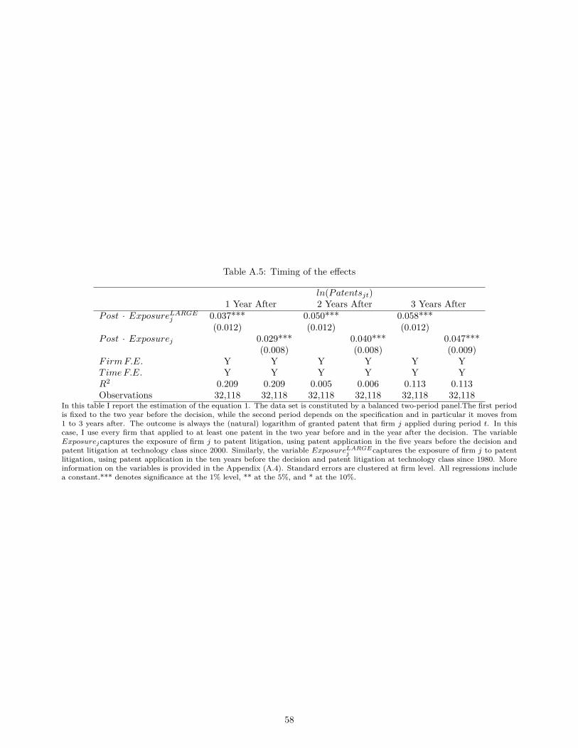
Table A.5: Timing of the effects

ln(Patentsjt)1 Year After 2 Years After 3 Years After

Post · ExposureLARGEj 0.037*** 0.050*** 0.058***(0.012) (0.012) (0.012)

Post · Exposurej 0.029*** 0.040*** 0.047***(0.008) (0.008) (0.009)

FirmF.E. Y Y Y Y Y YTimeF.E. Y Y Y Y Y YR2 0.209 0.209 0.005 0.006 0.113 0.113Observations 32,118 32,118 32,118 32,118 32,118 32,118

In this table I report the estimation of the equation 1. The data set is constituted by a balanced two-period panel.The first periodis fixed to the two year before the decision, while the second period depends on the specification and in particular it moves from1 to 3 years after. The outcome is always the (natural) logarithm of granted patent that firm j applied during period t. In thiscase, I use every firm that applied to at least one patent in the two year before and in the year after the decision. The variableExposurejcaptures the exposure of firm j to patent litigation, using patent application in the five years before the decision andpatent litigation at technology class since 2000. Similarly, the variable ExposureLARGE

j captures the exposure of firm j to patentlitigation, using patent application in the ten years before the decision and patent litigation at technology class since 1980. Moreinformation on the variables is provided in the Appendix (A.4). Standard errors are clustered at firm level. All regressions includea constant.*** denotes significance at the 1% level, ** at the 5%, and * at the 10%.

58

TableA.6:Rob

ustness:

diffe

rentiallineareff

ectbe

fore

andaftertheshock

(1)

(2)

(3)

(4)

(5)

ln(Patentsjt

+1)

Patentscaled

jt

1{Patent jt

=Top

10%}

1{Patent jt

=Top

25%}

Aver

age

Sca

led

Cit

ati

ons

Post·E

xposurej

0.011***

0.013***

0.004*

0.010***

0.025*

(0.004)

(0.003)

(0.002)

(0.003)

(0.014)

Pre·E

xposurej

0.003

0.002

0.001

0.001

0.013

(0.004)

(0.003)

(0.002)

(0.003)

(0.014)

FirmF.E.

YY

YY

YTimeF.E.

YY

YY

YIndu.×TimeF.E.

YY

YY

YR

20.001

0.010

0.001

0.002

0.00

1Observatio

ns257,024

257,024

257,024

257,024

257,024

Inthetable,

Irepo

rttheestimationof

anequa

tion

where

Iusetheda

taas

apa

nela

ndIestimatethesamespecification

asequa

tion

(1),bu

twhere

Iinteract

therisk

expo

sure

measure

withbo

thadu

mmyforafterthedecision

(equ

alto

oneforqu

arters

afterMay

15th

2006)an

dadu

mmyforthequ

arters

before

thedecision

.The

variab

leExposure jcaptures

the

expo

sure

offirmjto

patent

litigation,

usingpa

tent

applicationin

thefiv

eyearsbe

fore

thedecision

andpa

tent

litigationat

techno

logy

classsince2000.Therefore,theinteraction

compa

rescorporatebe

havior

before

andafterthedecision

tothebe

havior

inthequ

arterthat

concludedwiththedecision

.The

specification

isau

gmentedwithtechno

logy

trends,u

sing

themajor

techno

logy

ofthefirm

interacted

withprean

dpo

stdu

mmies.

The

data

setisconstitutedby

apa

nelw

itheigh

tqu

arteran

ditisba

lanced

inan

yspecification

.In

anycase,I

useeveryfirm

that

publishedat

leaston

epa

tent

inthetw

oyear

before

andin

theyear

afterthedecision

.Colum

n(1)ha

sthe(natural)logarithm

plus

oneof

gran

tedpa

tent

that

firm

jap

plieddu

ring

period

t.Colum

n(2)ha

sgran

tedpa

tent

that

firmjap

plieddu

ring

period

t,scaled

bythetotaln

umbe

rof

patentsin

thetw

oyearsbe

fore

thedecision

.Colum

ns(3)

and(4)ha

vethedu

mmywhich

isequa

ltoon

ewhether

thefirmjap

plieddu

ring

period

tat

leastto

onepa

tent

that

isin

thetop10%

or25%

ofthematched

patents(sam

eyear

and

sametechno

logy

class).Colum

n(5)ha

sthe(natural)logarithm

plus

oneof

gran

tedpa

tent

that

firmjap

plieddu

ring

period

tweigh

tedby

citation

sreceived

inthefirst

threeyearsof

life.

Citations

arescaled

bytheaverag

enu

mbe

rof

citation

sreceived

bythepa

tentsin

thesametechno

logy

classan

dyear.Moreinform

ationon

theda

tais

availablein

theApp

endix

(A.4).

Allregression

sinclud

eaconstant.Stan

dard

errors

areclusteredat

firm

level.Allregression

sinclud

eaconstant.***

deno

tessign

ificanceat

the1%

level,**

atthe5%

,and

*at

the10

%.

59

Table A.7: Timing of the effects

ln(Patentsjt)1 Year After 2 Years After 3 Years After

Post · Exposurej 0.002 0.037*** 0.051***(0.009) (0.009) (0.010)

Post · Exposurej · Computer 0.093*** 0.008 -0.004(0.019) (0.030) (0.022)

Post · ExposureLARGEJ 0.004 0.052*** 0.072***(0.013) (0.014) (0.010)

Post · ExposureLARGEj · Computer 0.085*** 0.016 -0.009(0.027) (0.029) (0.030)

FirmF.E. Y Y Y Y Y YTimeF.E. Y Y Y Y Y YR2 0.215 0.215 0.006 0.006 0.117 0.117Observations 32,128 32,128 32,128 32,128 32,128 32,128

In this table I report the estimation of the equation 1, where I interact the shock measure with a dummy for firms that are inthe Computer industry, as defined in Appendix A.4. The data set is constituted by a balanced two-period panel. The first periodis fixed to the two year before the decision, while the second period depends on the specification and in particular it moves from1 to 3 years after. The outcome is always the (natural) logarithm of granted patent that firm j applied during period t. In thiscase, I use every firm that published at least one patent in the two year before and in the year after the decision. The variableExposurejcaptures the exposure of firm j to patent litigation, using patent application in the five years before the decision andpatent litigation at technology class since 2000. Similarly, the variable ExposureLARGE

j captures the exposure of firm j to patentlitigation, using patent application in the ten years before the decision and patent litigation at technology class since 1980. Standarderrors are clustered at firm level. All regressions include a constant.*** denotes significance at the 1% level, ** at the 5%, and *at the 10%.

Table A.8: Robustness: differential linear effect before and after the shock

(1) (2) (3) (4)R&Djt/Assetjt

Post · ExposureLARGEj 0.004** 0.006**(0.002) (0.003)

Pre · ExposureLARGEj 0.001 0.001(0.002) (0.002)

Post · Exposurej 0.003** 0.004**(0.001) (0.001)

Pre · Exposurej 0.002 -0.001(0.001) (0.002)

Firm&TimeF.E. Y Y Y YIndu. × TimeF.E. Y YOther Controlsjt Y YR2 0.005 0.027 0.006 0.029Observations 16,272 16,272 16,272 16,272

In the table I report the estimation of an equation where I use the data as a panel and I estimate the same specification as equation(1), but where I interact the risk exposure measure with both a dummy for after the decision (equal to one for quarters after May15th 2006) and a dummy for the quarters before the decision. Therefore, the interaction compares corporate behavior before andafter the decision to the behavior in the quarter that concluded with the decision. The data set is constituted by a panel witheight quarter and it is balanced in any specification. The variable Exposurejcaptures the exposure of firm j to patent litigation,using patent application in the five years before the decision and patent litigation at technology class since 2000 and the variableExposureLARGE

j captures the exposure of firm j to patent litigation, using patent application in the ten years before the decisionand patent litigation at technology class since 1980. In any case, I use every firm that published at least one patent in the two yearbefore and in the one year after the decision. The table has have R&D/Asset , measured at quarterly frequency. The even columnsare augmented with industry, as constructed in the Appendix, interacted with time dummies (per quarter). More information onthe data is available in the Appendix (A.4). All regressions include a constant.*** denotes significance at the 1% level, ** at the5%, and * at the 10%.

60

TableA.9:Ev

iden

ceon

Patent

Mix:pre-trendan

alysis

(1)

(2)

(3)

(4)

ExtensiveMargin

IntensiveMargin

ln(Patentsjtr

)1{Patentsjtr>

0)Post·1{Riskr}

-0.019

-0.009

0.040***

0.027***

(0.017)

(0.015)

(0.002)

(0.002)

Pre·1{Riskr}

-0.016

0.0015

-0.002

0.001

(0.018)

(0.015)

(0.003)

(0.002)

Split

10%

25%

10%

25%

Firm×TimeF.E.

YY

YY

Firm×RiskF.E.

YY

YY

R2

0.924

0.913

0.688

0.687

Sample

2,785

3,893

54,844

54,844

Observatio

ns89,120

124,576

1,755,008

1,755,008

Thistableprov

ides

astud

yof

pre-trending

forresultsrepo

rted

inTa

ble(3).

Inorderto

doso,I

estimatethesamespecification

asbe

fore

witho

utcolla

psingtheda

taan

destimating

adiffe

rentialeff

ectforthetreatm

entbe

fore

andafterthedecision

.Dataareat

quarterlylevelin

afour

year

arou

ndthedecision

,foratotalof

16pe

riod

s.In

practice,Iestimate:

yj

tr=α

jr

+α

jt

+β

PO

ST

1{Risk

r}·Post

+β

PR

E1{Risk

r}·Pre,

where

whereα

jtisasetof

firm-tim

efix

edeff

ects,α

jrisasetof

fixed

effects

atfirm-group

level,

1{Risk

r}isadu

mmy

formoreriskygrou

ps.HerePost

identifiesqu

arters

afterthedecision

andPrethosebe

fore

thedecision

.The

quarterof

thede

cision

-20061-

isthereferencepe

riod

forinterpreting

thecoeffi

cients.Dataarereshap

edforthis

analysis

atthefirm-tim

e-riskinessgrou

plevel.

Inpractice,Igrou

ppa

tent

withinafirm

inacertaintimeacross

twoclassesdepe

ndingon

thelevelo

friskinessr,s

uchthatr

={highrisk

;lowrisk}.

Patents

areassign

edto

oneof

thetw

ogrou

psba

sedon

theintensity

oflitigationof

theirtechno

logy

classafter2000

based

ontheWestL

awLitiga

tion

data.In

particular,I

split

theda

taacross

both

10%

and25%.Iconsider

twoou

tcom

es:in

columns

(1)-(2)Iuseln

(pat j

tr),

which

isthelogarithm

ofthe

patent

applications

that

firmjfiled

todu

ring

timetin

theclassof

riskr.Sincethisshou

ldcapturetheintensivemarginof

thetreatm

ent,Iuseallfi

rmsthat

aresimultaneou

slyactive

inbo

thrisk

classes,

arou

ndthedecision

time.

Thislead

sto

asampleof

arou

nd3,000firmsdepe

ndingon

thesplit.Then,

incolumns

(3)-(4)Iha

vey

jtr

tobe

equa

lto

1{Pat j

tr>

0),

which

isadu

mmyequa

ltoon

eifthefirmjap

pliesto

anygran

tedpa

tent

inrisk-group

rat

timet.

Inthiscase,m

ysampleismuchlarger

andIconsider

everyfirm

that

hasap

pliedto

atleaston

epa

tent

inthetenyearsbe

fore

thedecision

.Stan

dard

errors

areclusteredat

firm

level.Allregression

sinclud

eaconstant.***

deno

tessign

ificanceat

the1%

level,**

atthe

5%,a

nd*at

the10

%.

61

Table A.10: Effect across defendant status

(1) (2) (3) (4) (5) (6)Public firms ln(Patentsjt)

LikelyDef. LikelyP laint. All LikelyDef. LikelyP laint. All

Post · Exposurej 0.0644* 0.0355 0.091* 0.107** 0.005 0.094**(0.0376) (0.0462) (0.048) (0.050) (0.101) (0.047)

Post · LikelyP laint.t -0.090 -0.063(0.073) (0.074)

Post · Exposurej · LikelyP laint. -0.029 -0.0071(0.059) (0.062)

FirmF.E. Y Y Y Y Y YT imeF.E. Y Y Y Y Y YIndu. × T imeF.E. Y Y YOther Controlsjt Y Y YR2 0.005 0.051 0.011 0.089 0.294 0.083Observations 1,642 392 2,034 1,642 392 2,034

(a) Public firms

(1) (2) (3) (4) (5) (6)Full Sample ln(Patentsjt)

LikelyDef. LikelyP laint. All LikelyDef. LikelyP laint. All

Post · Exposurej 0.043*** 0.019 0.019 0.040*** -0.037 0.037***(0.009) (0.033) (0.033) (0.011) (0.047) (0.034)

Post · LikelyP laint. -0.161*** -0.083**(0.04) (0.040)

Post · Exposurej · LikelyP laint. -0.023 -0.028(0.034) (0.034)

FirmF.E. Y Y Y Y Y YT imeF.E. Y Y Y Y Y YIndu. × T imeF.E. Y Y YOther Controlsjt Y Y YR2 0.007 0.021 0.008 0.033 0.123 0.034Observations 30,328 1,800 32,128 30,328 1,800 32,128

(b) Full SampleThese panels report the estimate of the linear difference-in-difference specification (equation 1), where I allow the effect of theexposure to the decision to be heterogeneous across firm likelihood of being a plaintiff at the time of the decision. The outcomeis always ln(Patentsjt), which is the log of the total number of patents over the period. As usual, this is winsorized at 1%. Thevariable Exposurejcaptures the exposure of firm j to patent litigation, using patent application in the five years before the decisionand patent litigation at technology class since 2000. The first panel reports the analysis on the sample of public companies. Thesecond panel instead reports the analysis over the full sample. The dummy Likely Plaintiff is equal to one if the firm has beeninvolved in more lawsuits as a plaintiff rather than a defendant. I first report the regressions as split between likely plaintiff andthe complementary group - which I call likely defendant -, and then I report the fully interacted regression in the whole sample.I always control for firm and time fixed effects, but in Columns (4)-(6) I add extra controls interacted with time dummies. As inthe previous analyses, I control for industry, location dummies of the firm, the size of the portfolio before the estimation period,a dummy for “start-up”, which in this context is firms that published the first patent in the three years before the decision, andaverage quality of the patent portfolio in the pre period, measured by average citations. More information on the data is availablein the Appendix (A.4). Standard errors are clustered at firm level. All regressions include a constant.*** denotes significance atthe 1% level, ** at the 5%, and * at the 10%.

62

Table A.11: Heterogeneity of the effects: growth

(1) (2) (3) (4)R&Djt/Assetjt

Standard ControlsGrowth Standard ControlsGrowthPost · Exposurej · SmallREV ENUEj 0.004** 0.004** 0.003* 0.003**

(0.002) (0.002) (0.002) (0.002)Post · Exposurej · SmallEMP

j 0.004** 0.004** 0.003 0.003*(0.002) (0.002) (0.002) (0.002)

Post · Exposurej · 1{Dividendj = 0} 0.005** 0.007*** 0.005* 0.007***(0.002) (0.002) (0.003) (0.002)

Post · Exposurej · 1{Ratingj = NO} 0.004** 0.003* 0.002 0.003(0.002) (0.002) (0.002) (0.002)

FirmF.E. & TimeF.E. Y Y Y YIndu. × TimeF.E. Y YOther Controlsjt Y YObservations 2,034 2,034 2,034 2,034

These Tables report the estimate of the coefficient β1 of the following equation:

yjt = αj + αt + β1(Exposurej ·FinConj ·Post) + β2(FinConj ·Post) + β3(Exposurej ·Post)

+β4(Growthj ·Post) + β5(Growthj ·FinConj ·Post) + γXjt + εjt

across different specifications. First, different rows measure financial constraint in different ways. In particular, I use: (1) size,as measure by firm below the median revenue in my sample; (2) size, as measure by firm below the median employment in mysample; (3) dividend, where I look at firms that paid no cash dividends in any quarters in the three years before the decision ; (4)rating, where I sort based on whether the firm has any rating. Second, in columns (1)-(3), I report the standard results I havealready reported, and in columns (2)-(4) I introduce a fully interacted control for firm growth over the pre-period. This measureis the simple growth of revenue over the two years of pre period. Even if not reported, all the regressions are estimated as fullyinteracted. The outcome is always R&D/Asset, which is the average over the period of the quarterly R&D expenses scaled by totalassets. As usual, this is winsorized at 1%. The variable Exposurejcaptures the exposure of firm j to patent litigation, using patentapplication in the five years before the decision and patent litigation at technology class since 2000. I always control for firm andtime fixed effects, but in Columns (4)-(6) I add extra controls interacted with time dummies. As in the previous analyses, I controlfor industry, location dummies of the firm, the size of the portfolio before the estimation period, a dummy for “start-up”, which inthis context is firms that published the first patent in the three years before the decision, and average quality of the patent portfolioin the pre period, measured by average citations. More information on the data is available in the Appendix (A.4). Standard errorsare clustered at firm level. All regressions include a constant.*** denotes significance at the 1% level, ** at the 5%, and * at the10%.

Table A.12: Stock Market returns and Litigation Exposure

EventDay Event [−1; +1] Event [0; +5] Event [−5;−1]Ret. A.Ret. Ret. A.Ret. Ret. A.Ret. Ret. A.Ret.

Exposurej 0.012*** 0.013*** 0.013*** 0.011*** 0.008** 0.006* 0.001 -0.001(0.004) (0.004) (0.003) (0.003) (0.004) (0.004) (0.003) (0.003)

Observations 986 986 986 986 986 986 986 986The table reports cross-sectional value-weighted regressions between litigation exposure and returns. Returns are measured eitherraw or as abnormal returns, where this is constructed as rj − βjr

S&P 500, where βare estimated by firm regressions between onemonths and twelve months before the decision. Furthermore, returns are measured over different windows, which are reported inthe header of the table. Returns are winsorized at 1%. The variable Exposurejcaptures the exposure of firm j to patent litigation,using patent application in the five years before the decision and patent litigation at technology class since 2000. The weights aregiven by the firm market value of equity seven days before the decision. Standard errors are robust to heteroskedasticity. More infoon the variables are provided in the Appendix (A.4). All regressions include a constant.*** denotes significance at the 1% level, **at the 5%, and * at the 10%.

63

A.2 Background information on “eBay versus MercExchange”

The main object of the dispute in the 2006 “eBay vs. MercExchange” case was a patent on the popular “Buy It

Now” function on the eBay platform.58 In the early 2000s, MercExchange accused eBay of infringing some of the

company’s online auction patents. In 2003, the Virginia Circuit Court agreed with these accusations, but then

decided to reject MercExchange’s request to issue an injunction on eBay’s technologies (Court, 2003). However,

this decision was subsequently reversed by the Court of Appeals, which clearly stated that the issuance of a

permanent injunction, “absent exceptional circumstances,” was a general rule in the U.S. intellectual property

enforcement system. In 2005, eBay decided to petition this decision in front of the Supreme Court, which agreed

to discuss the case in the following year. As I discuss in the paper, the final ruling of the Court rejects the idea

that injunction should always be issued in normal cases after a patent violation.

The opinion of the Court of Appeals was not surprising before 2006, as injunction was issued almost auto-

matically after a violation was proved. This idea dates back to a 1908 Supreme Court case between Continental

Paper Bag and Eastern Paper Bag (Court, 1908). In this case, the Supreme Court clearly states that “exclusion

may be said to have been of the very essence of the right conferred by the patent, as it is the privilege of any

owner of property to use or not use it, without question of motive.” In practice, the only cases where a firm would

not receive injunction is when the firm could successfully argue in favor of the public interest of its products.

Otherwise, the ruling granted to patent owner full ability to exclude others from using the technologies covered

by the patent.

A.3 The timing of the decision

The ruling should affect the trajectory of innovation only if it was not anticipated by agents in this market.59

In this section I argue that this was the case using different pieces of qualitative evidence from news sources

and other public records. This is consistent with the large body of research in law that discusses the decision

(e.g. Bessen and Meurer 2008a; Holte 2015; Shapiro 2010; Tang 2006; Venkatesan 2009)

As a first step, I have reviewed the news about the case and I did not find any evidence that the content

of the ruling was anticipated. This is the case both when looking at news published in the weeks before the

decision and right after it. If anything, the outcome of the decision appeared surprising for the news of the

day.60 Furthermore, I have examined specifically different set of individuals that had some direct “skin in

the game” in the decision. First, the Justices appeared to be divided during the oral hearing. For instance,58The patent is USPTO number 5,845,265.59The activities of the Supreme Court are planned in advanced and therefore the general public knew that the case “eBay vs.

MercExchange” was under review. At the time, there was not an exact calendar, but generally there was agreement that the finaldecision was going to be taken most likely by the end of June. See, for instance, the article “Supreme Court to Take AnotherLook at "Automatic" Injunctions for Prevailing Patent Owners in Infringement Cases”, appeared online December 12th 2005 in theMondaq Business Briefing, a news provider for legal expert.

60MarketWatch defined the ruling “a surprising turn” of the Court. MarketWatch was accessed through Bloomberg “SupremeCourt Rules for eBay in Patent Case: Expert Lawyer Calls Decision Surprising,” May 15th 2006

64

Patently-O, one of the most reputable patent law blogs, claimed that “based on oral arguments, pundits see a

potential split decision in the eBay v. MercExchange injunction case.”61 In particular, Justice Scalia appeared

to be in favor of considering an injunction as automatic after an infringement: “we’re talking about a property

right here, and a property right is the exclusive right to exclude others.” Interestingly, in the end the Supreme

Court made the decision unanimously. Second, in the weeks before the decisions, the government took a clear

stand against eBay, and therefore in disagreement with what the Court later decided. In particular, on March

10th – two weeks before the oral argument of the case - the Office of the Solicitor General (OSG), on behalf

of both the Federal Trade Commission and the antitrust division of the Justice Department, asked to confirm

the injunction to eBay.62 While the opinions of the OSG are in no way binding for the Supreme Court, they

have an impact on the public perception of these issues. Third, even the business community was split on this

issue. While large drug companies were opposing any change in the way injunction was issued, large companies

in high tech – such as Intel, Cisco, Hewlett-Packard, Microsoft– were explicitly supportive of eBay.63

A.4 Data

A.4.1 Samples

This is a more detailed clarification on Section (3) in the paper, where I discuss the data and variable construc-

tion.

Firm level data comes from two sources. Patent data comes from the Fung Institute (University of California

at Berkeley),64 and they are an updated version of the Harvard Business School Patent Network Database (Li

et al., 2014). In particular, I use all the assigned granted patents in the data, for which there are not missing

information on the grant date, application date, assignee ID and technology class.65 It is worthy to point out

that all analyses are carried based on application date, since I am interested in capturing a date closer to the

time of an investment. The data were download in August 2014 and they contain all patents that were granted

before 29th April 2014. For the full sample, I define a firm based on the assignee identifiers in the data for

the analysis using the full set of innovative firms. For this identifier, I rely on the ID provided by the original

Fung Institute data, based on name disambiguity (Li et al., 2014). To evaluate quality of the data, I compare

them to the aggregate statistics that USPTO provides online.66 In particular, I compare patents granted to

corporations according to USPTO aggregate data to the data used in this paper. I find that the two series61See the article “eBay v. MercExchange Oral Arguments,” from March 31st 2006, which can be found at the following address

http://patentlyo.com/patent/2006/03/ebay_v_mercexch_3.html62See for reference, Washington Post article on this issue “Government Sides Against eBay in Patent Dis-

pute,” March 11th 2006. A copy is available online at the following link: http://www.washingtonpost.com/wp-dyn/content/article/2006/03/10/AR2006031001918.html

63Helm (2006) argues that these difference stems from the different use of injunction for large firms across these industries.64Data can be found: http://funginstitute.berkeley.edu/tools-and-data (downloaded in August 2014)65To minimize the loss of information, I have supplemented missing information on the dates and technology class with data

from Google USPTO patent data, which were nicely shared with me by Josh Feng.66Table can be found here: http://www.uspto.gov/web/offices/ac/ido/oeip/taf/h_at.htm#PartA2_1

65

almost overlap across the whole period and strongly co-move over 2002-2008 period. In the year, where they

differ the most, the difference is only about of 2%.67

Most of the analyses in the paper are carried using a sample of innovative firms, which are firms active in

patenting before and after the decision. In particular, I define innovative firms as firms that applied to at least

one patent in the two years before the decision and one in the year after this. The advantage of this approach

is to have a sample that is the same when analyzing different sample period (one, two or three years after the

decision). Furthermore, this sample is intrinsically balanced when I do the analysis considering data collapsed

before and after the decision. When I am interested in the intensive margin, I need to consider a larger set of

firms. In particular, I take firms that have at least one patent in the four years before the decision, but not

necessarily anything afterwards.

In the second part of this work, I supplement patent level data with information on R&D at firm level for

the subset of innovative firms, for which public information are available. Data on firms’ financials come from

Compustat quarterly data. This allows me to construct pre and post period windows that are exactly around

the Supreme Court decision. In order to add patent information to Compustat data, I use the data provided

in Kogan et al. (2012). I construct a bridge file which is based on patent ID: this approach does not have the

concerns of a matching performed by name. Essentially, I match the two data sets based on USPTO patent ID

- as defined in the Fung Institute data - and then I use this match to bridge the assignee IDs to the ID used

in Kogan et al. (2012). Since the assignee ID in the patent data is based on name disambiguity, one firm in

patent data may correspond to more than one company ID in Compustat: therefore, the analysis at firm level

use the more aggregate Compustat ID (gvkey). Furthermore, in about 90% of the cases, the company ID in

the patent data corresponds to only one Compustat ID. In the remaining cases, I use the Compustat ID that

received more unique matching over the period considered. An hand-check of the data supports the quality of

this choice.

The final sample in the public firm data set is subject to some standard filters. In particular, I focus on

non-financial companies and non-government related companies, with the headquarter in USA. Furthermore, I

exclude firms that do not have a balance reporting around the decision. In particular, while some data entry may

be missing for acceptable reasons, total assets and revenue should always be populated. I therefore eliminate

those firms that do not have balance reporting on these variables in the four-year symmetric window around

the shock, which is the same period I use for the analyses. Furthermore, I want to exclude those companies that

may be under financial distress or restructuring: in order to do this, I exclude companies that systematically

report negative equity over the usual period. Lastly, as in the rest of the paper, I focus only on innovative firms.

All in all, I have a sample of more than one thousand firms. Using the Compustat IDs, I then also match the67This difference can stem from two things. First, it is not super clear how USPTO categorize companies, so there may be some

discrepancy in this dimension. Second, the aggregate data looks at patent granted at a time different than April 2014. Third, partof difference is probably made up of patents that had missing info in the micro data, such as missing date or technology.

66

firm to stock returns information from CRSP.

In the end, as discussed in Section (3), I use patent lawsuits data from public filings to construct the measure

of litigation size at technology class level. The data are collected from WestLaw, a subsidiary of Thomson

Reuters. Westlaw is one of the primary provider of legal data in United States and use public records to

develop a complete overview of lawsuits in United States. The same data, also known as Derwent LitAlert data,

were previously used by other empirical work on patent litigation (e.g. Lerner 2006; Lanjouw and Schankerman

2001).

Using the online tool LitAlert, I searched for all the litigation involving patents between 1980 and 2006.68

Every filing should report the date of the filing, the plaintiffs, the defendants and information on the intellectual

property that is used to go to court. As a preliminary step, I eliminate the few filings with missing information

about the date. To avoid issues with duplicates, I keep only one case in situations where multiple observations

share the same entries for plaintiff, defendant, filing data and patents. Since I am interested in utility patents,

at this point I keep only filings that report at least one utility patent. As discussed in Section (3), I make filings

comparable across each other by reshaping the data at plaintiff-defendant-patent level. Then, I match patents

with their technology fields and I aggregate them at technology class level over different periods of time. Lastly,

I use equation (3) to construct the final score at technology class level.

A.4.2 Variables definition

In the analysis involving the full sample of innovative firms, I use various outcomes.

For measuring intensity of innovation, I look at two measures. First, I look at the logarithm of the patents

produced by the firm j at time t, ln(patjt), which is consistent to an intensive margin of our treatment. Using

this outcome, I consider the sample of every firm, either private or public, which applied to at least one patent

before and after the shock, as previously discussed. In this sample, there are slightly more than 16 thousand

firms that satisfy this condition. Consistent with the literature, I count patents weighting them based on the

number of assignee to which the patent is granted. In particular, I weight assignee equally. However, results

are completely unaffected when I use a normal patent count, where I count patents as one even when assigned

to multiple parties. Second, in order to estimate something closer to an extensive margin of the treatment, I

consider an alternative outcome variable, which is a dummy equal to one when the firm has applied to any

granted patent in the period, 1{Patentjt > 0}. In order to measure exposure to litigation for a firm, this has to

have to at least one (applied) patent before the shock. Because of this, as I discussed before, I consider the set

of firms that has at least one patent in the four years before the Supreme Court decision, for a total of around

77 thousand firms.69 Results do not change if I shrink the window by looking only at three years before the68http://intranetsolutions.westlaw.com/practicepages/template/ip_litalert.asp?rs=IPP2.0&vr=1.069The outcome variable is constructed looking only at the two years before and after the shock, as in the intensive margin

measure.

67

decision or I increase it to six years before the decision.

For measuring quality of innovation, I construct few metrics based on patent citations. Following the

literature in this area, I count patent citations at a fixed window -3 years - after the granting (e.g. Bernstein,

2015). I then construct various outcomes based on this. I consider two main outcomes. First, I measure the

average quality of the portfolio, by looking at the average number of adjusted citations. The citation adjustment

is made to take care of the fact that the number of citations is highly heterogeneous across technology and across

time. Following the literature, I make citations comparable by scaling them by the average number of citation

received by a patent of the same vintage and technology class (Lerner and Seru, 2015). Second, I look at the

probability that a company applies to patents that are at the top of the citation distribution in the relevant

reference group as a proxy for breakthrough innovation. The reference group is composed by assigned patents

that are the same USPTO technology class and were developed by the company in the same year, based on

application date. I then look at whether the company has applied to any patent which is on the top 10% and

25% of the distribution of citations.

To analyze defensive patents, I also construct two other patent based measures. First, I measure the share

of defensive patents by counting the number of patents that have low quality – measured by forward citations

– but whose patent claim spans a very large set of different technologies, measured by originality (Hall et al.,

2001). In practice, my outcome - which I refer as share of defensive patents - is the share of granted patent

applications that are in the top 25% in terms of originality among patents of same technology class and year,

despite being in the bottom three quartiles in terms of citations for the same group. Second, I also construct a

measure of the share of business method patents, looking at both patents are specifically in the business method

category (class 705) or using a broader definition developed in Hall (2003).70

I also use the patent data to construct a set of other controls. I construct a new measure of industry of

the firm, which is based on patent application, rather than self-reporting industry. The main advantage of this

measure is that I can use it both across public and private firms. Firm j is assigned to a certain industry by

looking at the major industry in which the firm has applied to the highest number of patents. In line with the

literature, major industries are defined as in the Appendix (1) of Hall et al. (2001). I use patents in the four

years around the decision for the analysis. Similarly, I define a measure of location of the firm based on patent

data. In particular, I assigned to firm j the location c if location c is the modal location for the patents applied

in the four years before the Supreme Court decision. An extra code is used for firms for which no state location

can be determined. I also construct a measure of size of the portfolio of the firm in question, looking at patents

that were filled in the two years before the estimation window. The reason I use patent over this period is that I

cannot use patenting before the decision inside the estimation window because this measure would be collinear

with the outcomes.70The list of these other technology classes is in Hall (2003) Table 3. In particular, these are technology classes: 84, 119, 379,

434, 472, 380, 382, 395, 700, 701, 702, 703, 704, 705, 706, 707, 709, 710, 711, 712, 713, 714, 715, 717, 902.

68

In the second part of the paper, I then use a set of balance sheets variables. All balance sheet ratios

are winsorize at 1% to ensure that results are not driven by outliers. My main measure of R&D intensity is

R&D/Asset. R&D expenditure is measured using quarterly Compustat data (variable xrdq) and it is adjusted

for acquisition of in process R&D expenses (variable rdipq), as in Mann (2013). Notice than the adjustment

does not produce first-order effects in the outcome, as the share of firm-quarter with non-zero in process R&D

expenses is, as expected, very small. The quarterly data are augmented, if necessary, with yearly data. These

data are consistently adjusted at quarterly level assuming equal R&D across quarters within the fiscal year.

Lastly, in line with the literature, missing R&D data is replaced with zero.

A.4.3 Matching lawsuits to firm

This section explains how I identify in the data those patenting companies that were more likely to be plaintiff

at the time of the ruling.71 The first step is to match companies by name across the assignee names available

in the patent data and the information on plaintiff and defendant from Westlaw. Specifically, I use Westlaw to

generate two lists of companies involved in patent litigation – one for defendant and one for plaintiff companies

– using the fillings between 2001 and 2005. There are a number of challenges in establishing this link. The

primary challenge is the lack of standardization in the name of firm across the datasets. For example, a firm

may be listed in the patent dataset as “The XYZ Company,” while in the defendant dataset, the same firm is

listed as “XYZ, LLC.” Firms in the two data sets may be part of the same economic group, but file for patent or

litigation under a different legal entity. Additionally, there may also be cases of firms’ names that are incorrectly

transcribed.

To address these concerns, we use a combination of automatic and manual matching techniques. Each of the

following procedures are performed for the plaintiff and defendant separately. First, we use automatic matching

to divide the sample of plaintiffs in different groups depending whether a matching is sure, likely or unlikely.

Using “pandas” package for Python 3.5, we clean every name in each dataset by first removing all punctuation

and common abbreviations, such as AG, BV, INC, LLC, LTD, etc. The same cleaning procedure is applied

to both patent and litigation data. Each cleaned name in the defendant (plaintiff) set was compared with the

every cleaned name in the patent data via the “quick_ratio()” function of the “SequenceMatcher” class in the

“difflib” package for Python 3.5. This procedure returns a number between 0 and 1 that measures the similarity

between two strings. If the similarity was above 0.9, the two strings are said to be a probable match and are

marked as such. If the two strings had a computed similarity of less than, or equal to 0.9, they are said to be an

unlikely match and are marked as such. After this automatic matching, a final manual matching is completed

using a research assistant. First, we assume that the pair where similarity equal to one is a true matching.

Then, we manually look at the other pairs, with particular interests to those that were categorize as a probable71I greatly thank Matthew Nicholas Nicholson for his assistance in this data collection.

69

match (similarity above 0.9). As we find firms in the plaintiff and defendant lists that have a counterparty in

the patent data, we also link this to the correspondent assignee ID in the patent data.

After completing this matching process, I use the information collected to construct a dummy that determines

whether a company is more likely to be a plaintiff at the time of the ruling. Specifically, this variable is equal

to one if the firm has been involved in more litigation fillings during 2001-2005 as a plaintiff, rather than a

defendant. For exposition purposes, I define the complementary group as the set of firms that are more likely

to be defendant rather than plaintiffs.

A.4.4 Stock Market data

When dealing with stock market data, I usually report the results both as raw returns and abnormal returns.

Raw returns are simply computed based on the standard stock returns. Abnormal returns are instead

constructed relative to a benchmark, which is usually either the S&P500 or the NASDAQ. The S&P500 returns

are also obtained from CRSP, while the NASDAQ data are obtained online from Yahoo Finance. In order

to construct abnormal returns, I compute the predicted returns estimating the β of each stock using daily

returns between 343 trading days before (January 1st 2005) and 30 trading days before the events. Conditional

on providing a sufficiently large window to estimate the β precisely, results are not affected by the choice of

the estimation window. When considering cumulative returns, I compute them as simple sum of the returns.

Furthermore, when I use value-weights, I compute the weights based on equity capitalization seven trading days

before the decision and keep them constant throughout.72

When I test the returns of NPEs around the event I report t-statistic, that tests the difference of the

average returns from zero. This is constructed based on heteroskedasticity robust errors, and the estimation is

implemented for simplicity using least-squares.

A.5 Other analyses

A.5.1 Permutation test

As quickly presented in Section 5), I develop a permutation test (Chetty et al. 2009; Fisher 1922) as a further

robustness on my results. With this test, I compare the t-statistic from my analysis to a non-parametric

distribution of statistics that I obtain by randomly assigning technology classes to firm. The objective of this

test is twofold. First, this methodology allows me to provide inference based on weaker assumptions than

the standard linear model. Second, this test can be used to evaluate whether my analysis is capturing some

other spurious firm characteristic that is different than litigation exposure but somehow correlated with it. For

instance, this analysis allows me to reject that my results are somehow driven mechanically by the way the

exposure index is constructed.72I use the stock price and the number of shares provided by CRSP to compute the market value of equity.

70

The intuition for this test is simple: if my results correctly capture the exposure to litigation through the

technology fields, I would expect to find no results when technology exposure is randomly assigned. Rather than

a one-to-one comparison, I implement this test by constructing a full distribution of test statistics obtained in

this way. If my model is correctly capturing true exposure to patent litigation, I would expect the true statistic

to be on the top percentiles of this distribution.

In short, the procedure is implemented in the following way: I start by re-assigning randomly the technology

classes in which a company operates for every firm in the sample.73 Then, based on this, I reconstruct the

exposure index Exposurej and I run the main specification presented before. I repeat this procedure for a

thousand random iterations and then I plot the non-parametric distribution of the t-statistic I obtain from this.

I compute the p-value of my true model by looking at the percentile in which my true t-statistic is within the

constructed distribution. As expected, I find that the p-value constructed based on the random permutation

test is similar to the standard one, and lower than 1% (Figure 6). Also this test confirms the quality of my

empirical framework.

A.5.2 Supreme Court decision and stock prices

In the end, I examine the stock market reaction of innovative firms around the decision. Overall, I find that firms

that were more exposed to litigation experienced a small, positive out-performance right around the decision.

Consistent with the previous results, I interpret this result as confirming that the decision was able to reduce

the burden of litigation on innovative public firms.74

Previous research in finance has shown that innovation can positively affect the stock market valuation of

firms (Kogan et al., 2012). If this is the case, an improvement in the enforcement of patents should positively

affect the stock prices of innovative firms. This should be particularly the case for companies for which this

dimension is particularly relevant, such as firms that operate in areas where patent litigation is intense. One

caveat on this setting - which we will discuss more later - is that investors may not be immediately aware of the

effects of the decision on innovation.75 In order to study this question, I measure returns and abnormal returns

around the announcement and I correlate these measures with the measure of litigation exposure. Then, I test

how these returns correlate with the measures of exposure to litigation. Consistent with the previous results, I

would expect an out-performance of firms operating in technologies that are more intensively litigated.

The main result of the analysis can be synthesized by Figure (A.6), which plots the cumulative value-weighted

returns of high and low exposure firms, where the split is made at the top 25% of the litigation distribution.73For instance, a firm that has obtained two patents in class 131 (Tobacco) and three in 428 (Stock material or miscellaneous

articles) can be assigned to have two patents in class 432 (Heating) and three in 125 (Stone working).74See section A.4.4 in the Appendix for more info on data construction and analysis.75In particular, with respect to the effect on non-practicing entities (NPE), the consequences of the decision on standard innovative

firms may be harder to identify. First, while the decision had an unambiguous, negative effect on NPEs, the impact of the rulingon innovation is less clear ex ante (section 2.3). Second, a change in patent enforcement is clearly more salient for non-practicingentities.

71

I find that the two groups behave in the same way in the days before the ruling. However, the day of the

decision, the high-risk group outperforms the low-risk group by almost 1%. This out performance does not

revert afterwards, and the two groups seem to present similar growth rates in the following dates.

In Table (A.12), I explore the same issue within a regression framework, where I run cross-sectional value-

weighted regression between firm returns and ex-ante exposure to litigation. As usual, I focus on the sample of

innovative public firms for which I find return information on CRSP around the time of decision. In columns (1)

and (2), I find that companies that are more exposed to litigation performed better on the day of the decision. A

one-standard deviation difference in exposure translates in 1% difference in returns. The results are essentially

identical for both raw and abnormal returns. Furthermore, I obtain very similar coefficients when I look at a

one-day window around the event (columns 3 and 4). This fact confirms that most of the movement in stock

prices happen on the first day after the ruling was made public. I also show that the results are similar – albeit

a bit smaller – when using the returns from the entire week after the decision (columns 5 and 6). Lastly, a

formal test in columns 7 and 8 also rejects the presence of differential returns across firms in the week prior to

the decision, confirming that the results were not driven by differential trends in returns.

These results are consistent with those presented earlier on the stock returns of nonpracticing entities.

Altogether, they confirm that the ruling negatively affected the market value of firms that generate most of

the revenue through litigation activity but it had a positive effects on innovative firms that operate in litigious

areas. The only difference between the results is that for NPE some of the negative effects can also be seen

on the trading day before the news. One explanation for this difference is that the content of the decision was

uncertain, but it was known that the Supreme Court was going to release a decision soon. This effect may have

triggered an increase in uncertainty for NPE, for which the decision was more salient and riskier.

72