Risks of Large Portfolios

Jianqing Fan ∗†, Yuan Liao‡ and Xiaofeng Shi∗

∗Department of Operations Research and Financial Engineering, Princeton University

† Bendheim Center for Finance, Princeton University

‡ Department of Mathematics, University of Maryland

Abstract

Estimating and assessing the risk of a large portfolio is an important topic in finan-

cial econometrics and risk management. The risk is often estimated by a substitution

of a good estimator of the volatility matrix. However, the accuracy of such a risk esti-

mator for large portfolios is largely unknown, and a simple inequality in the previous

literature gives an infeasible upper bound for the estimation error. In addition, numer-

ical studies illustrate that this upper bound is very crude. In this paper, we propose

factor-based risk estimators under a large amount of assets, and introduce a high-

confidence level upper bound (H-CLUB) to assess the accuracy of the risk estimation.

The H-CLUB is constructed based on three different estimates of the volatility matrix:

sample covariance, approximate factor model with known factors, and unknown factors

(POET, Fan, Liao and Mincheva, 2013). For the first time in the literature, we derive

the limiting distribution of the estimated risks in high dimensionality. Our numeri-

cal results demonstrate that the proposed upper bounds significantly outperform the

traditional crude bounds, and provide insightful assessment of the estimation of the

portfolio risks. In addition, our simulated results quantify the relative error in the risk

estimation, which is usually negligible using 3-month daily data. Finally, the proposed

methods are applied to an empirical study.

Keywords: High dimensionality, approximate factor model, unknown factors, principal

components, sparse matrix, thresholding, risk management, volatility

∗Address: Department of Operations Research and Financial Engineering, Sherrerd Hall, Princeton Uni-versity, Princeton, NJ 08544, USA, e-mail: jqfan@princeton.edu, yuanliao@umd.edu, xshi@princeton.edu.The research was partially supported by DMS-1206464 and NIH R01GM100474-03, NIH R01-GM072611-08.

1

arX

iv:1

302.

0926

v1 [

stat

.AP]

5 F

eb 2

013

1 Introduction

The potential of a portfolio’s loss is termed as the portfolio risk. There are two types of

portfolio risks. The systematic risk (or market risk) is the risk inherent to the entire market,

such as risk associated with interest rates, currencies, recession, war and political instability,

etc. The systematic risk cannot be diversified away, even with a well-diversified portfolio.

In contrast, specific risk (or idiosyncratic risk) refers to the risk that affects a very specific

group of securities or even an individual security. For example, it can be the risk of price

changes due to the unique circumstances of a specific stock. Unlike systematic risk, specific

risk can be reduced through diversification.

Estimating and assessing the risk of a large portfolio is an important topic in financial

econometrics and risk management. The risk of a given portfolio allocation vector w is

conveniently measured by (w′Σw)1/2, in which Σ is a volatility (covariance) matrix of the

assets’ returns. Often multiple portfolio risks are at interests and hence it is essential to

estimate the volatility matrix Σ. The problem becomes challenging when the portfolio size

is large. Suppose we have created a portfolio from two thousand assets and invested in a

part of selected assets. The covariance matrix Σ involved then contains over two million

unknown parameters. Yet, the sample size based on one year’s daily data is around 252. It

is hard to assess the estimation accuracy when the estimation errors from more than two

million parameters are aggregated. Hence some regularization method is recommended to

estimate and assess risks.

The interest on large portfolios surges recently. Pesaran and Zaffaroni (2008) examined

the asymptotic behavior of the portfolio weights. Brodie et al. (2009) addressed the problem

of portfolio selection using a regularization penalty. Gomez and Gallon (2011) numerically

compared several methods of covariance matrix estimation for portfolio management. In

particular, the optimal portfolio selection involves inverting an estimated Σ, which is a

challenging problem under a large number of assets. The literature is also found in Jacquier

and Polson (2010), Antoine (2011), Chang and Tsay (2010), DeMiguel et al. (2009), Ledoit

and Wolf (2003), El Karoui (2010), Lai et al. (2011), Bannouh et al. (2012), Gandy and

Veraart (2012), Bianchi and Carvalho (2011), among others.

This paper contributes to the literature in at least four aspects. First of all, we propose

risk estimators based on factor analysis. Traditionally Σ is estimated by the sample covari-

ance. However, when the number of assets is larger than the sample size, it is well known

that the sample covariance is singular, which may result in an estimated risk being zero for

certain portfolios. By assuming a factor structure on the returns, we obtain strictly positive

definite covariance estimators Σ even when the number of assets is larger than the sample

2

size. Two factor-based methods are proposed. The first estimator assumes the factors to be

known and observable. The second method deals with the case in which common factors are

unknown. This is particularly important for analyzing many non-U.S. markets when assets’

returns are driven by a few unknown factors. In both cases, the factor model imposes a

conditionally sparse structure, in that the idiosyncratic covariance is a large sparse matrix.

This yields to an approximate factor model as in Chamberlain and Rothschild (1983), with

a non-diagonal error covariance matrix.

Secondly, we provide a new and practical method to assess the accuracy of risk estimation

w′(Σ−Σ)w. In the literature (e.g., Fan et al. 2012), this term has been bounded by

ξT = ‖w‖21‖Σ−Σ‖max

where ‖w‖1, the L1-norm of w, is the gross exposure of the portfolio, which is bounded when

there are no extreme positions in the portfolio. However, this upper bound depends on the

unknown Σ, hence is not applicable in practice. In addition, the numerical studies in this

paper demonstrate that this upper bound is too crude: it is often of the same or even larger

scale than the estimated risk. In contrast, we provide a high-confidence level upper bound

(H-CLUB) for w′(Σ−Σ)w, which is of much smaller scale and easy to compute in practice.

H-CLUB is constructed based on the confidence interval for the true risk. For each proposed

risk estimator w′Σw and a given τ ∈ (0, 1), we find an H-CLUB U(τ) such that

P (|w′(Σ−Σ)w| ≤ U(τ))→ 1− τ.

In contrast, P (|w′(Σ − Σ)w| ≤ ξT ) = 1. Hence H-CLUB is an upper bound for the risk

estimation error with high confidence while the traditional bound ξT is of full confidence.

The third contribution is that for the first time in the literature, we derive the inferential

theory of the risk estimators with a high-dimensional portfolio, especially when the estimator

is factor-based with either observed or unobserved factors. Although factor analysis has long

been used for the portfolio allocation theory, it remains largely unknown whether the effects

of estimating the factor loadings and unobservable factors are negligible in risk estimation,

especially when the dimensionality is high. This paper proves that these effects are indeed

asymptotically negligible for diversified portfolios, even when the dimensionality is much

larger than the sample size. Interestingly, we find that when the dimensionality is larger

than the sample size, the factor-based risk estimators have the same asymptotic variances

no matter whether the factors are known or not, and they are asymptotically equivalent.

Hence the high dimensionality is in fact a bless for risk estimation instead of a curse from

this point of view. In addition, the asymptotic variance of factor-based estimators is slightly

3

smaller than that of the sample covariance-based estimator, but the difference is small. This

demonstrates that the benefit of using a factor model is not in terms of a much smaller

asymptotic variance, because the systematic risk cannot be diversified. Rather, factor anal-

ysis gives a strictly positive definite covariance estimator, which is essential to estimate the

optimal portfolio allocation vector, and also interprets the structure of the portfolio risks.

Finally, using our simulated results based on the model calibrated from the real U.S.

equity market data, we are able to quantify the relative error of the estimation error or

coefficient of variation, defined as STD(w′Σw)/w′Σw, where STD(·) denotes the standard

error of the estimated risk. Interestingly, this ratio is just a few percent and is approximately

independent of the gross exposure ‖w‖1 but sensitive to the length of the time series. On

the other hand, we also quantify the relation between the crude bound and the practical

H-CLUB. We find that ξT is many times larger than U(τ), and the ratio ξT/U(τ) increases

as the gross exposure increases.

We also contribute to the portfolio theory by introducing a sampling technique which

picks a random portfolio with a given gross exposure level. This sampling scheme can be

useful for portfolio optimization and understanding the overall risks within a given level of

gross exposure.

We emphasize that the recent works by Fan et al. (2011, 2013) are only concerned about

covariance estimations and no inferential theories were studied. In contrast, we focus on

the risk estimation, with a particular attention to the risk assessment and the impact of

covariance estimation on the limiting distributions of risk estimators.

The rest of the paper is organized as follows. Section 2 proposes new risk estimators

based on factor analysis under both known and unknown factor cases. Section 3 constructs

the H-CLUB for each risk estimator based on the confidence interval for risks. It also derives

the limiting distributions of the risk estimators and compares their asymptotic variances.

Section 4 presents simulation results. An empirical study is considered in Section 5. Finally,

Section 6 concludes. All the proofs are given in the appendix.

Throughout the paper, ‖w‖1 =∑N

i=1 |wi| is used to denote the gross exposure of a

given portfolio allocation vector. For a square matrix A, λmin(A) and λmax(A) represent its

minimum and maximum eigenvalues. Let ‖A‖max and ‖A‖ denote its element-wise sup-norm

and operator norm, given by ‖A‖max = maxi,j |Aij| and ‖A‖ = λ1/2max(A′A) respectively.

2 Estimation of Portfolio’s Risks

LetRtTt=1 be a time series of an N×1 vector of observed asset returns and Σ = cov(Rt),

often known as the volatility matrix. The portfolio risk of a given allocation vector w is

4

given by√

var(w′Rt), which is√

w′Σw. How to estimate the risk of a large portfolio? A

straightforward answer is√

w′Σw with an estimator Σ. But, how good is it? How to assess

the accuracy of this estimator? We address the problem or risk estimation in this section.

The assessment of the estimation accuracy will be discussed in Section 3.

The problem of estimating the risk of a given portfolio is challenging due to the high

dimensionality of Σ. Often the number of assets can be of hundreds or even thousands. On

the other hand, to adapt to the current market condition, a short period of financial data are

often used. For example, the number of daily returns in three months is only of tens. Hence

N can be much larger than T . We assume Σ to be time-invariant within a short period,

which holds approximately for locally stationary time series.

We consider three estimators for estimating var(w′Rt) for a given w, based on three

different estimators Σ: sample covariance estimator, factor analysis with either observed or

unobserved factors. Recently, Chang and Tsay (2010) proposed a Cholesky decomposition

approach to estimate the large covariance matrix, and used simulation to assess its perfor-

mance. On the other hand, the assets’ returns are usually driven by a few market factors.

Due to the presence of these common factors, Σ itself is not sparse. Moreover, as pointed out

by Stock and Watson (2002) and Bai (2003), common factors are usually pervasive, so the

factor loading matrix is not sparse either. Hence the factor-based risk estimators are widely

applicable in analyzing financial data, whose asymptotic properties (as both T,N →∞) will

be also presented below.

2.1 Sample-covariance-based estimator

The first estimator Σ = S is the conventional sample covariance matrix based on RtTt=1.

The asymptotic impact of using S on the risk management has been studied by Fan et al.

(2008, 2012) when N is much larger than T . The sample covariance estimator does not

require any structural assumption on the assets’ returns. It was shown by the aforementioned

authors that for a given portfolio w with a bounded gross exposure (that is, ‖w‖1 is bounded),

w′(S−Σ)w = Op(

√logN

T).

However, when N > T , it is well known that S is singular, and therefore may result in an

estimated risk being zero for certain portfolios.

5

2.2 Estimating risks based on factor analysis

To overcome the problem of singularity of the sample covariance under high dimensional-

ity, we assume that Rt satisfies an “approximate factor model” (Chamberlain and Rothschild

1983):

Rt = Bft + ut, t ≤ T, (2.1)

where B is an N ×K matrix of factor loadings; ft is a K × 1 vector of common factors, and

ut is an N × 1 vector of idiosyncratic error components. In contrast to N and T , here K

is assumed to be fixed. The common factors may or may not be observable. For example,

Fama and French (1992, 1993) identified three known factors that have successfully described

the U.S. stock market. In addition, macroeconomic and financial market variables have been

thought to capture systematic risks as observable factors. On the other hand, in an empirical

study, Bai and Ng (2002) determined two unobservable factors for stocks traded on the New

York Stock Exchange during 1994-1998.

Let cov(ft) and Σu = cov(ut) denote the covariance matrices of ft and ut, K × K and

N ×N respectively. Suppose ft and ut are uncorrelated. The factor model then implies the

following decomposition of Σ:

Σ = Bcov(ft)B′ + Σu.

Sparsity is one of the most common structures for large covariance estimation, which as-

sumes many off-diagonal elements of the covariance to be either zero or nearly so. In the

approximate factor model, a natural assumption is to place a sparse structure on Σu. The

rationale is, after the common factors are taken out, the remaining idiosyncratic components

should be mostly weakly correlated with each other. Such a condition is called conditional

sparsity. We now propose new risk estimators based on the conditional sparsity assumption.

2.2.1 Factor-based estimator

We first assume that the common factors are observable, and construct an estimator of

Σ based on thresholding on the covariance matrix of idiosyncratic errors. Suppose B is the

least squares estimator of B. The residual sample covariance matrix of ut is then given by

Su = T−1T∑t=1

utu′t = (Su,ij)N×N , ut = Rt − Bft.

6

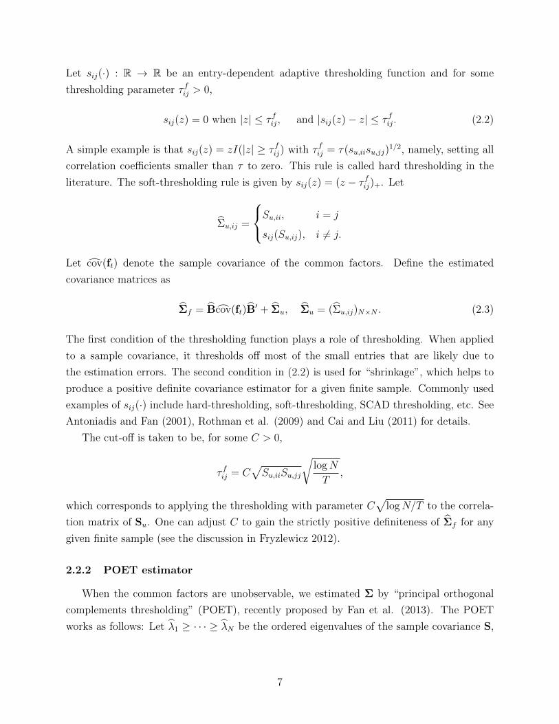
Let sij(·) : R → R be an entry-dependent adaptive thresholding function and for some

thresholding parameter τ fij > 0,

sij(z) = 0 when |z| ≤ τ fij, and |sij(z)− z| ≤ τ fij. (2.2)

A simple example is that sij(z) = zI(|z| ≥ τ fij) with τ fij = τ(su,iisu,jj)1/2, namely, setting all

correlation coefficients smaller than τ to zero. This rule is called hard thresholding in the

literature. The soft-thresholding rule is given by sij(z) = (z − τ fij)+. Let

Σu,ij =

Su,ii, i = j

sij(Su,ij), i 6= j.

Let cov(ft) denote the sample covariance of the common factors. Define the estimated

covariance matrices as

Σf = Bcov(ft)B′ + Σu, Σu = (Σu,ij)N×N . (2.3)

The first condition of the thresholding function plays a role of thresholding. When applied

to a sample covariance, it thresholds off most of the small entries that are likely due to

the estimation errors. The second condition in (2.2) is used for “shrinkage”, which helps to

produce a positive definite covariance estimator for a given finite sample. Commonly used

examples of sij(·) include hard-thresholding, soft-thresholding, SCAD thresholding, etc. See

Antoniadis and Fan (2001), Rothman et al. (2009) and Cai and Liu (2011) for details.

The cut-off is taken to be, for some C > 0,

τ fij = C√Su,iiSu,jj

√logN

T,

which corresponds to applying the thresholding with parameter C√

logN/T to the correla-

tion matrix of Su. One can adjust C to gain the strictly positive definiteness of Σf for any

given finite sample (see the discussion in Fryzlewicz 2012).

2.2.2 POET estimator

When the common factors are unobservable, we estimated Σ by “principal orthogonal

complements thresholding” (POET), recently proposed by Fan et al. (2013). The POET

works as follows: Let λ1 ≥ · · · ≥ λN be the ordered eigenvalues of the sample covariance S,

7

whose corresponding eigenvectors are denoted by ξjNj=1. We then estimate Σ by

ΣP =K∑j=1

λj ξj ξ′j + Ω, Ω = (Ωij)N×N , Ωij =

∑N

k=K+1 λkξ2k,i, i = j

sij(∑N

k=K+1 λkξk,iξk,j), i 6= j.

where sij(·) is the same adaptive thresholding function as before, based on an entry-

dependent threshold τPij :

τPij = C√

ΩiiΩjj

(√logN

T+

1√N

).

Recall that K denotes the number of common factors. Here C is a user-specified constant

to maintain the finite sample positive definiteness. Thanks to the thresholding, even when

T = o(N), there is C∗ > 0 such that for any C > C∗, both Σf and ΣP are strictly positive

definite with probability approaching to one. Simulated and empirical studies suggested that

C = 0.5 is a good choice when sij is the soft thresholding.

Based on the factor analysis, our proposed risk estimator is either

√w′Σfw or

√w′ΣPw

for a given portfolio allocation vector w, depending on whether ft is observable. Note that

Fan et al. (2013) is concerned only about the covariance estimation. In contrast, this

paper focuses on the asymptotic behaviors of these risk estimators and their assessment

for a given diversified w, which have never been addressed before. We will see that under

high dimensionality, the factor-based estimators have the same asymptotic variance, and is

smaller than that of the sample covariance-based estimator. The effect of estimating the

unknown factors on the limiting distributions is asymptotically negligible.

3 Assessment of the Risk Estimation

This section proposes a new method to assess the estimated risks for a given portfolio

allocation vector w. We will assume ‖w‖1 ≤ c for some c > 0, where ‖w‖1 is the gross

exposure of the portfolio. This prevents extreme positions.

3.1 Measuring risks using full confidence bound

As described in Section 2, we use a covariance estimator to form a risk estimator w′Σw.

A natural question then arises: how close is the estimated risk to the true risk? In other

words, how do we assess ∆ = |w′(Σ−Σ)w|? Technically this question is challenging under

high dimensionality. A simple inequality as ∆ ≤ ‖w‖2‖Σ−Σ‖ would not give a convergence

8

upper bound when N is large. An alternative (and commonly used) upper bound for ∆ is

based on the following inequality:

∆ ≤ ‖w‖21‖Σ−Σ‖max ≡ ξT , (3.1)

which is usually tighter for risk assessment.

However, for the purposes of statistical inference, ξT is infeasible as it depends on the

true Σ. As a result, this upper bound cannot be evaluated in practice for a given data set.

In addition, our simulation results have shown that the upper bound ξT is actually too crude

to be useful. Let us consider the following toy example.

Example 3.1. Consider three stocks with annualized returns that jointly follow a multi-

variate Gaussian distribution N3(0,Σ) where Σ = 0.04 · I3. An equally weighted portfolio

w = (1/3, 1/3, 1/3)′ is constructed and the task is to estimate the portfolio risk using the

sample covariance matrix S based on the simulated 21-day (one month) returns.

The theoretical value of portfolio variance is w′Σw = 0.0133, which corresponds to a

true risk of 11.55% per annum. Based on a typical simulated data, the estimated portfolio

variance wΣw = 0.0131, equivalent to a perceived risk of 11.43% per annum. Moreover

ξT = ‖Σ − Σ‖max = 0.0248. Based on this upper bound, a simple calculation shows that

w′Σw ∈ [0, 0.0379], that is, the true risk√

w′Σw lies in [0, 19.46%], an interval that is too

wide to be meaningful.

Note that the inequality (3.1) holds for every sampling sequence RtTt=1. Hence ξT is in

fact an upper bound of full confidence, that is,

P (|w′(Σ−Σ)w| ≤ ξT ) = 1.

The toy example is typical in the sense that ξT is already too crude for small portfolios. In

statistical inference, often people use bounds of high confidence levels instead, e.g., quantities

that bound ∆ with a high probability. This paper pursues such a high-confidence-level upper

bound (H-CLUB) based on the confidence interval.

3.2 H-CLUB

We propose a new confidence upper bound for ∆ = |w′(Σ−Σ)w| to assess the estimation

error of the portfolio risks. More specifically, for each proposed matrix estimator Σ and any

given τ > 0, we find a quantity U(τ) such that for all large N and T ,

P (|w′(Σ−Σ)w| ≤ U(τ)) ≥ 1− τ.

9

Therefore, U(τ) is an asymptotic (1 − τ)100% confidence upper bound for ∆. In addition,

it is data-driven (up to user-specified tuning parameters), hence can be easily calculated in

practice and used to construct confidence intervals for the true risks.

Before proceeding, we make a technical comment that one needs to be careful about the

limiting behaviors of T and N . In this paper, we will treat N as an increasing function of

T . Hence N grows via a fixed trajectory, e.g., N = NT = Tα for some α > 0, and can be

faster than T , namely, α > 1. As a result, we need to apply the triangular array central

limit theorem with weakly dependent time series data.

3.3 Sample covariance based risk estimator

Let us start with the sample covariance matrix of Rt. For simplicity and exposition, let

us assume that the returns have mean zero and S = T−1∑T

t=1 RtR′t. We make the following

assumptions, under which the serial dependence across t is allowed.

Assumption 3.1. (i) RtTt=1 is strictly stationary with ERt = 0 and cov(Rt) = Σ.

(ii) There is M > 0 such that maxi≤N E|Rit|8 ≤M.

Let us introduce the strong mixing condition. Let F0−∞(R) and F∞T (R) denote the σ-

algebras generated by Rt : −∞ ≤ t ≤ 0 and Rt : T ≤ t ≤ ∞ respectively. In addition,

define the mixing coefficient αR(T ) = supA∈F0−∞(R),B∈F∞T (R) |P (A)P (B)− P (AB)|.

Define the autoregressive function γT (h) = cov((w′Rt)2, (w′Rt+h)

2), which depends on

T through dim(w) = N = NT . Let

σ2T = γT (0) + 2

∞∑h=1

γT (h). (3.2)

Assumption 3.2. (i) There exists r0 > 0 and M > 0 such that: for all T ∈ Z+,

αR(T ) ≤ exp(−MT r0).

(ii)∑∞

h=1 |γT (h)| = O(1),∑T

h=1 hγT (h)/T = o(σ2T ) and αR(T ) = o(γT (0)).

Assumption 3.2 requires the weak dependence of the time series. Strong mixing con-

dition is assumed. The first two conditions in (ii) are usually mild. When a diversified

w is used, the last condition in (ii) is easy to satisfy as long as the dimensionality is not

exponentially large in T because the mixing coefficient is assumed to decay exponentially

fast. To illustrate its meaning, consider a simple case where w = (1/N, · · · , 1/N), then

γT (0) = var(( 1N

∑Ni=1Rit)

2), which is in general no smaller than O(N−c) for some c > 0.

10

Due to the strong mixing condition in Assumption 3.2(i), αR(T ) = o(γT (0)) if N = NT

grows at a polynomial rate of T .

We are now ready to define the H-CLUB for the estimation error w′(S−Σ)w. Let

γ(h) = T−1T−h∑t=1

((w′Rt)2 −w′Sw)((w′Rt+h)

2 −w′Sw).

In particular, γ(0) = T−1∑T

t=1(w′Rt)

4 − (w′Sw)2. Let zτ/2 denote the upper τ/2 quantile

of the standard normal distribution. For some increasing sequence L = L(T )→∞, let

σ2 = γ(0) + 2L∑h=1

γ(h), US(τ) = zτ/2√σ2/T . (3.3)

Here L is a truncation parameter, and as L slowly increases, σ2 consistently estimates σ2T .

Lemma 3.1. Under Assumptions 3.1-3.2,

|σ2 − σ2T | = Op(L

3/2T−1/2 +∑h>L

γT (h)),

If in addition L3 = o(Tσ4T ) and

∑h>L γ(h) = o(σ2

T ), then

|σ2 − σ2T | = op(σ

2T ) and US(τ) = o

(√logN

T

).

The following theorem gives the limiting distribution of the estimated risk. It also demon-

strates that US(τ) is a valid H-CLUB for |w′(S− Σ)w|.

Theorem 3.1. Under the assumptions of Lemma 3.1, as T,N →∞,[var

(T∑t=1

(w′Rt)2

)]−1/2Tw′(S−Σ)w→d N (0, 1),

and for any τ > 0,

P(|w′(S−Σ)w| ≤ US(τ)

)→ 1− τ.

As a result U(τ) = zτ/2√σ2/T is an H-CLUB with confidence level (1 − τ)100% and is

data-driven once a user-specified L is determined. Compared to the traditional bound ξT ,

US(τ) can be easily calculated for any given time series data. The scale of US(τ) is much

smaller than that of ξT . Our simulation results show that even for a small τ (e.g., τ = 0.01),

the magnitude of U(τ) is much smaller than the crude bound ξT . (See Table 3 in Section 4.)

11

By the δ-method, we have the following corollary for the risk estimation. Define

R(w) =√

w′Sw, R(w) =√

w′Σw.

Corollary 3.1. Under the assumptions of Lemma 3.1, for any τ > 0, as T,N →∞,

P(|R(w)−R(w)| ≤ US(τ)/

√4w′Sw

)→ 1− τ.

3.4 Factor-based risk estimator

Let us now approach the problem via factor analysis. We assume

Rt = Bft + ut, (3.4)

where in this section, ftTt=1 are observed common factors. In the approximate factor model,

the idiosyncratic covariance Σu is non-diagonal. However, the risk component w′(Σu−Σu)w

introduced by the idiosyncratic error can be diversified away by a selected portfolio allocation

vector. Hence the estimation error of the risk only comes from the systematic error brought

by the common factors. Compared to the sample covariance based risk estimator, factor

analysis always gives strictly positive risk estimators even when N > T for any nonzero

allocation vector w.

For the factor-based risk estimation, a different set of assumptions are needed instead of

those in Section 3.3. First of all, the factor model is assumed to be conditionally sparse, in

the sense that Σu is a sparse matrix. We employ the approximate sparsity assumption in

Bickel and Levina (2008) as follows:

Assumption 3.3. There is q ∈ [0, 1) such that

sN ≡ maxi≤N

N∑j=1

|Σu,ij|q = o(min(T/ logN)(1−q)/2, N (1−q)/2).

When q = 0 we define sN = maxi≤N∑N

j=1 I(Σu,ij 6= 0) as the maximum number of nonva-

nishing elements in each row, and the assumption requires that sN = o((T/ logN)1/2, N1/2).

Assumption 3.3, though slightly stronger than those in Chamberlain and Rothschild (1983),

is quite meaningful in practice. For example, when the idiosyncratic components represent

firms’ individual shocks, they are either uncorrelated or weakly correlated among the firms

across different industries, because the industry specific components are not pervasive for

the whole economy (Connor and Korajczyk 1993).

12

Assumption 3.4. (i) ut, ftTt=1 is strictly stationary, utTt=1 and ftTt=1 are independent,

and Euit = Efjt = 0 for all i, j.

(ii) There exist r1, r2 > 0 and b1, b2 > 0, such that for any s > 0, i ≤ p and j,

P (|uit| > s) ≤ exp(−(s/b1)r1), P (|fjt| > s) ≤ exp(−(s/b2)

r2).

(iii) There is C > 0 such that C−1 < λmin(Σu) ≤ λmax(Σu) < C, maxi≤N ER2it < C,

‖B‖max < C and λmin(cov(ft)) > C−1.

Let F0−∞ and F∞T denote the σ-algebras generated by (ft,ut) : −∞ ≤ t ≤ 0

and (ft,ut) : T ≤ t ≤ ∞ respectively. Define the mixing coefficient αf (T ) =

supA∈F0−∞,B∈F∞T |P (A)P (B)− P (AB)|. Let

γf (h) = cov((w′Bft)2, (w′Bft+h)

2)

for h ≥ 0. It follows from the α-mixing condition that∑∞

h=1 |γf (h)| = O(1) (see Lemma B.5

in the appendix). In addition, define

σ2f = γf (0) + 2

∞∑h=1

γf (h). (3.5)

Assumption 3.5. (i) There exists r3 > 0 and M > 0 satisfying: for all T ∈ Z+,

αf (T ) ≤ exp(−MT r3).

(ii)∑∞

h=1 hγf (h)/T = o(σ2f ) and αf (T ) = o(γf (0)) as T,N →∞.

Assumption 3.6. w′Σuw = o(σ4f + σfT

−q/2(logN)−(1−q)/2s−1N ).

Note that σ4f = O(1). This assumption allows σ4

f to decay as N increases due to diversified

allocation vectors. Recall that q is defined in Assumption 3.3. Assumption 3.6 requires

‖w‖ = o(1), which assumes a diversified portfolio to reduce the idiosyncratic risk. To

illustrate the intuition, consider the following simple example.

Example 3.2. Consider a one-factor model on the asset returns:

Rit = bift + uit

where var(f 2t ) > 0 and Σu is a diagonal matrix. Hence q = 0 and sN = 1. For simplicity,

suppose ftTt=1 are independent across t, and thus σ2f = γf (0) = (w′B)4var(f 2

t ). As the

13

eigenvalues of Σu are bounded away from zero and infinity, Assumption 3.6 is equivalent to:

w′w = o((w′B)8 + (w′B)2/√

logN), (3.6)

which holds if w is “diversified” enough. For example, the equal-weight allocation w =

(1/N, · · · , 1/N) gives w′Σuw = O(N−1). Writing CN = |N−1∑N

i=1 bi|, then (3.6) holds as

long as N−1√

logN = o(C8N). This is true since CN is often bounded away from zero.

To construct H-CLUB, we need to first estimate γf (h). For cov(ft) = T−1∑T

t=1 ftf′t,

define

γf (h) = T−1T−h∑t=1

[(w′Bft+h)2 −w′Bcov(ft)B

′w][(w′Bft)2 −w′Bcov(ft)B

′w],

where B is the least squares estimator of B. For some L = L(T ), define

σ2f = γf (0) + 2

L∑l=1

γf (h), Uf (τ) = zτ/2

√σ2f/T . (3.7)

Let β = 3r−11 + 1.5r−12 + r−13 .

Lemma 3.2. Suppose (logN)2β+2 = o(T ) and L√

(L+ logN)/T +∑

h>L γf (h) = o(σ2f ).

Under Assumptions 3.3-3.6,

|σ2f − σ2

f | = Op(L

√L+ logN

T+∑h>L

γf (h)),

and

Uf (τ) = o

(√logN

T

).

Hence the H-CLUB has a smaller stochastic order than that of the crude bound ξT .

The following theorem shows that Uf (τ) is a valid H-CLUB for the risk estimation error,

and can be computed easily from the data in practice. Technically, Theorems 3.2 and 3.3

(to be introduced in the next subsection) below are not simple applications of the triangular

array central limit theorem. We need to show that after thresholding, the idiosyncratic risk

can be diversified away by the portfolio vector w, and the estimation error for the factor

loadings is asymptotically negligible even under high dimensionality.

Theorem 3.2. Suppose that the common factors are observable, and that the thresholded

Σf (2.3) is used as the covariance estimator. Under the assumptions of Lemma 3.2, as

14

T,N →∞, [var

(T∑t=1

(w′Bft)2

)]−1/2Tw′(Σf −Σ)w→d N (0, 1),

and for any τ > 0,

P(|w′(Σf −Σ)w| ≤ Uf (τ)

)→ 1− τ.

Remark 3.1. Similar to Corollary 3.1, if we use Rf (w) =

√w′Σfw to estimate R(w) =√

w′Σw, then applying a delta method gives

P

(|Rf (w)−R(w)| ≤ Uf (τ)/

√4w′Σfw

)→ 1− τ.

Hence Uf (τ)/

√4w′Σfw is a valid H-CLUB for |Rf (w)−R(w)|.

It is interesting to compare Uf (τ) with US(τ) and see if knowing the factor structure

results in a reduced upper bound. This is equivalent to comparing σ2 in (3.3) with σ2f in

(3.7). Essentially we are to compare the asymptotic variances of the estimated risks between

a pure nonparametric risk estimator (sample covariance) and an estimator based on factor

analysis. We will see in the following section that when the factor structure is specified, the

factor-based risk estimator indeed gives a slightly smaller asymptotic variance.

3.5 Risk estimation with unknown factors

Often the market assets’ returns are driven by a few unknown factors. Hence the common

factors ft may not be observable which makes the analysis more practical and challenging.

In this case, we apply the POET estimator for Σ to handle the difficulty of not knowing the

factors:

ΣP =K∑j=1

λj ξj ξ′j + Ω (3.8)

with K being the number of common factors. For simplicity, we will assume K to be known,

and in practice it can be estimated consistently using the BIC method (Bai and Ng 2002).

Then K in the above estimator can be replaced with its consistent estimator.

Under the conditional sparsity condition, Fan et al. (2011, 2013) showed that

‖Σ−1P −Σ−1‖ = Op

(sN

(logN

T+

1

N

)1/2−q/2)

(3.9)

15

and when common factors are observable,

‖Σ−1f −Σ−1‖ = Op

(sN

(logN

T

)1/2−q/2)

(3.10)

where q and sN are defined in Assumption 3.3. The term 1/N in (3.9) is the price for not

knowing ft. When T = o(N logN), the above convergence rates are the same. Intuitively, as

the dimensionality increases, more information about the common factors is collected, and

eventually the common factors can be treated as though they are known. Moreover, both

ΣP and Σf are strictly positive definite for all large N and T .

We will see that with large enough pool of assets and a diversified portfolio allocation,

the effect of estimating the unknown factors on the estimated risk is negligible. As a result,

w′ΣPw and w′Σfw have the same asymptotic limiting distribution. For this purpose, we

impose additional conditions.

Assumption 3.7. As N →∞, the eigenvalues of B′B/N are bounded away from both zero

and infinity.

Intuitively, Assumption 3.7 means that the common factors should be pervasive, that is,

impact on a non-vanishing proportion of individual time series. It implies that the first K

eigenvalues of Σ are growing with rate O(N), which are well separated from the eigenvalues

of Σu. For identification, we assume cov(ft) = IK and B′B to be diagonal. Consequently,

Σ = BB′ + Σu.

Write B = (b1, · · · ,bN)′. The following assumption is common in the literature of high-

dimensional factor analysis, e.g., Bai and Ng (2002), Bai (2003).

Assumption 3.8. There is M > 0 such that E[N−1/2(u′sut − Eu′sut)]4 < M and

E‖N−1/2∑N

i=1 biuit‖4 < M .

Motivated by (3.9) and (3.10), we require T = o(N logN) so that the effect of estimating

the common factors is first-order negligible. This is often true for the asset returns’ time

series data. In addition, the portfolio vector w should still be diversified enough. This leads

to the following assumption:

Assumption 3.9. σ2fT →∞, σ2

fN/T →∞, and w′Σuw = o(√σ2fs−1N N1/2−q/2T−1/2).

Assumption 3.9 can be verified similarly by an example like Example 3.2.

To define an H-CLUB for a factor model with unknown factors, we first apply the principal

components method (Stock and Watson 2002 and Bai 2003) to estimate σ2f . Let F =

16

(f1, · · · , fT ) be a K×T matrix such that the rows of F/√T are the eigenvectors corresponding

to the K largest eigenvalues of the T × T matrix R′R, where R = (R1, · · · ,RT ). Let

B = RF′/T . Define

γP (h) = T−1T−h∑t=1

[(w′Bft+h)2 −w′BB′w][(w′Bft)

2 −w′BB′w].

For some L = L(T )→∞, let

σ2P = γP (0) + 2

L∑h=1

γP (h), UP (τ) = zτ/2

√σ2P/T . (3.11)

Lemma 3.3. Suppose L = o(√Nσ2

f ). Under Assumptions 3.3-3.9,

|σ2P − σ2

f | = Op(L

√L+ logN

T+

L√N

+∑h>L

γf (h)) = op(σ2f ).

and

UP (τ) = o

(√logN

T

).

The following theorem shows that UP (τ) is an H-CLUB for w′(ΣP − Σ)w, and can be

computed easily from the data. Interestingly, w′ΣPw and w′Σfw have the same asymptotic

limiting distribution. The price paid for not knowing the factors is asymptotically negligible.

Theorem 3.3. Suppose the common factors are unobservable, and ΣP (3.8) is used as the

covariance estimator. Under the assumptions of Lemma 3.3, as T,N →∞,[var

(T∑t=1

(w′Bft)2

)]−1/2Tw′(ΣP −Σ)w→d N (0, 1),

and for any τ > 0,

P(|w′(ΣP −Σ)w| ≤ UP (τ)

)→ 1− τ.

Remark 3.2. Similarly, if we define RP (w) =

√w′ΣPw, then UP (τ)/

√4w′ΣPw is a valid

H-CLUB for |RP (w)−R(w)|.

Knowing the factor-structure of the return Rt improves the estimation efficiency relative

to the sample covariance estimator. This is demonstrated by the following theorem.

17

Theorem 3.4. Under the assumptions of Theorem 3.3,

var

[T∑t=1

(w′Rt)2

]> var

[T∑t=1

(w′Bft)2

].

The difference of the above two variances is actually small when w is diversified enough,

and this fact is further verified by our simulation results (see Tables 3 and 4 in Section 4). The

reason is that the systematic risk cannot be diversified. On the other hand, factor analysis

gives a strictly positive definite covariance estimator, whereas the sample covariance may

produce a risk estimator being zero for certain portfolio allocation vectors. The positive

definiteness is particularly important to estimate the optimal portfolio allocation vector.

Furthermore, factor analysis interprets the structure of portfolio’s risks. It is clearly seen

that the idiosyncratic risks can be diversified away by the portfolio allocation.

4 Monte Carlo Examples

In this section, we examine the finite-sample performance of both the full confidence

upper bound ξT defined in (3.1) and H-CLUB, based on three covariance estimators Σ,

using portfolios w with different gross exposure constraints. Graphical and numerical results

illustrate that ξT is indeed a very crude bound and H-CLUB has much better performance

in general. The number of factors and length of time are both fixed with K = 3 and T = 300

respectively. The dimensionality N gradually increases from 20 to 600.

Excess returns of the ith stock of a portfolio over the risk-free interest rate, yit, is assumed

to follow the Fama-French three-factor model [Fama and French(1992)]:

yit = λi1f1t + λi2f2t + λi3f3t + uit.

The first factor is the excess return of the whole equity market, while the second and third

factors are SMB (“small minus big” cap) and HML (“high minus low” book/price) respec-

tively. Using US equity market data, we calibrate a submodel to generate the loadings

bi = (λi1, λi2, λi3)′, the idiosyncratic noises ut and the factors ft = (f1t, f2t, f3t)

′.

4.1 Calibration

To calibrate parameters in the model, we use the data on daily returns of S&P 500’s top

100 constituents ranked by market capitalization (on June 29th 2012), the data on 3-month

Treasury bill rates, and daily return data of the Fama-French factors. They are obtained

18

from COMPUSTAT database, the data library of Kenneth French’s website, and CRSP

database respectively. The excess returns (yt, ft) are analyzed for the period from July 1st,

2008 to June 29th 2012, approximately 1000 trading days.

(1) Calculate the least square estimator B of yt = Bft+ut, and compute the sample mean

vector µB and sample covariance matrix ΣB of all the row vectors of B. These parameters are

reported in Table 1. The factor loadings biNi=1 of the simulated models are then generated

from a trivariate Gaussian distribution N3(µB,ΣB).

µB ΣB

0.9833 0.0921 -0.0178 0.0436-0.1233 -0.0178 0.0862 -0.02110.0839 0.0436 -0.0211 0.7624

Table 1: Mean and covariance used to generate bi

(2) Assume that the factors follow the stationary vector autoregressive VAR(1) model

ft = µ + Φft−1 + εt for some 3 × 3 matrix Φ, where εt follows i.i.d N3(0,Σε). The model

parameters Φ,µ and Σε are calibrated using the daily excess returns of the Fama-French

factors ft. The covariance matrix cov(ft) is then obtained by solving the linear equation

cov(ft) = Φcov(ft)Φ′ + Σε. Results are summarized in Table 2.

µ Φ cov(ft)0.0260 -0.1006 0.2803 -0.0365 3.2351 0.1783 0.77830.0211 -0.0191 -0.0944 0.0186 0.1783 0.5069 0.0102-0.0043 0.0116 -0.0272 0.0272 0.7783 0.0102 0.6586

Table 2: Parameters used to generate ft

(3) The error covariance matrix is sparse in our setting. For each fixed N , it is created

by Σu = DΣ0D, where D = diag(σ1, · · · , σp). To be more specific, σ1, · · · , σp are generated

independently from a Gamma distribution G(α, β), in which α and β are selected to match

the sample mean and sample standard deviation of the 100 standard deviations of the errors

ut = yt − Bft (recall that each ut is 100 dimensional). An additional restriction is imposed

on σi that only values in between the minimum and maximum of the standard deviation

of ut are accepted. We then generate the off-diagonal entries of the correlation matrix Σ0

independently from a Gaussian distribution, with mean and standard deviation equal to

those of the sample correlations of the estimated residuals. Moreover, absolute values of the

off-diagonal entries are set to no greater than 0.95. Finally the hard-thresholding is applied

to make Σ0 sparse, where the threshold is set to be the smallest constant that makes Σ0

positive definite.

19

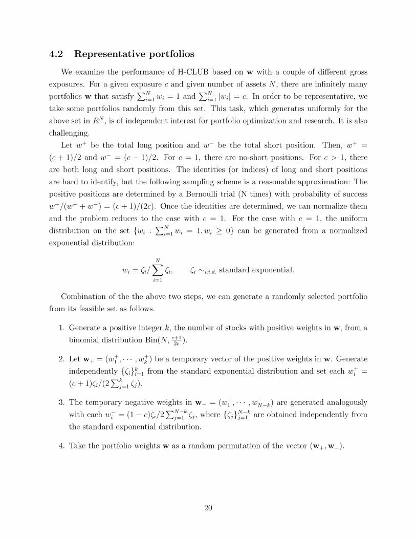
4.2 Representative portfolios

We examine the performance of H-CLUB based on w with a couple of different gross

exposures. For a given exposure c and given number of assets N , there are infinitely many

portfolios w that satisfy∑N

i=1wi = 1 and∑N

i=1 |wi| = c. In order to be representative, we

take some portfolios randomly from this set. This task, which generates uniformly for the

above set in RN , is of independent interest for portfolio optimization and research. It is also

challenging.

Let w+ be the total long position and w− be the total short position. Then, w+ =

(c + 1)/2 and w− = (c − 1)/2. For c = 1, there are no-short positions. For c > 1, there

are both long and short positions. The identities (or indices) of long and short positions

are hard to identify, but the following sampling scheme is a reasonable approximation: The

positive positions are determined by a Bernoulli trial (N times) with probability of success

w+/(w+ + w−) = (c + 1)/(2c). Once the identities are determined, we can normalize them

and the problem reduces to the case with c = 1. For the case with c = 1, the uniform

distribution on the set wi :∑N

i=1wi = 1, wi ≥ 0 can be generated from a normalized

exponential distribution:

wi = ζi/N∑i=1

ζi, ζi ∼i.i.d. standard exponential.

Combination of the the above two steps, we can generate a randomly selected portfolio

from its feasible set as follows.

1. Generate a positive integer k, the number of stocks with positive weights in w, from a

binomial distribution Bin(N, c+12c

).

2. Let w+ = (w+1 , · · · , w+

k ) be a temporary vector of the positive weights in w. Generate

independently ζiki=1 from the standard exponential distribution and set each w+i =

(c+ 1)ζi/(2∑k

j=1 ζj).

3. The temporary negative weights in w− = (w−1 , · · · , w−N−k) are generated analogously

with each w−i = (1− c)ζi/2∑N−k

j=1 ζj, where ζjN−kj=1 are obtained independently from

the standard exponential distribution.

4. Take the portfolio weights w as a random permutation of the vector (w+,w−).

20

4.3 Simulation

For each simulation with a given c, we fix T = 300 and gradually increase N from 20 to

600 in a multiple of 20. For each fixed N , we use 50 different model parameters and 200

testing portfolios for each given set of model parameters so that a total of 10,000 portfolios

were actually used. In other words, we iterate the following steps for 50 times, record values

of R(w),∆ = |w′(Σ − Σ)w|, ξT and U(τ), and compute their own means and standard

deviations. The details are summarized as follows:

1. Generate biNi=1 independently from N3(µB,ΣB). Set B = (b1, · · · ,bp)′.

2. Generate utTt=1 independently from Np(0,Σu).

3. Generate ftTt=1 from a VAR(1) model ft = µ+ Φft−1 + εt with parameters specified

in the calibration part.

4. Calculate yt = Bft + ut for t = 1, · · · , T .

5. Calculate the sample covariance matrix S = T−1∑T

t=1(yt − y)(yt − y)′; obtain the

factor-based covariance estimator Σf by using the hard-thresholding rule with the

threshold ωT = 0.10K√

logN/T ; and get the POET covariance estimator ΣP using

the soft-thresholding with thresholding parameter 0.5√

ΩiiΩjj(√

logNT

+ 1√N

).

6. Generate 200 w according to the method described in Section 4.2.

7. Over the 200 generated portfolios w, compute the average of true risk R(w) =√

w′Σw;

Also for Σ = S, Σf and ΣP , compute their respective average of ∆ = |w′(Σ −Σ)w|,ξT = ‖w‖21‖Σ − Σ‖max and U(0.05) = 2

√σ2/T . In our setting, the number of lags

L = 5.

Under several gross exposure constraints c, we produce the graph of risk domain by

plotting R(w) as a function of c and N (20 to 600 in increments of 20). Averages of ∆, ξT

and U(0.05) are also plotted against N , for all three types of covariance estimators Σ. We

will observe from the graphs that portfolios with larger c are exposed to have higher risks.

Finally, we fix the dimensionality N = 600 and the number of simulation replications is

now set to 500. Values of two ratios are recorded, namely ratio of bounds

RE1 =ξT

U(0.05)=‖w‖21‖Σ−Σ‖max

2

√var(w′Σw)

,

21

and relative error

RE2 =U(0.05)

4w′Σw=

√var(w′Σw)

2w′Σw.

This is computed for c in a practical range of [1, 2] and for several lengths of the time series.

The means and standard deviations of the two ratios are summarized in tables below.

4.4 Results

In Figure 1, averages of annualized true risks R(w) of 10000 portfolios 50 sets of model

parameters are plotted against dimensionality N . Multiple curves with different settings on

c are produced for comparison purpose. As shown in the figure, average of the actual risk

ranges from less than 30% to around 50% per annum, as c varies from 1 to 4 and N gradually

grows from 20 to 600.

Figure 1: Averages of annualized risks R(w) with ‖w‖1 = 1, 2, 3 and 4, over 10000 portfolios.

0 100 200 300 400 500 600

30

35

40

45

N

An

nualiz

ed R

isk (

%)

The Risk Domain

c=1

c=2

c=3

c=4

The following two observations can be made from Figure 1:

(1) The average risk is higher for a larger exposure parameter c. This is consistent with

the fact that portfolios with greater gross exposure are more volatile, and hence incur

higher risk.

(2) Given a gross exposure level c, as the portfolio size N increases, the average risk

decreases. The rate of decline is very fast until N is around 150. This is consistent

22

with the theory that as N increases, the portfolio becomes more diversified and the

idiosyncratic risk is reduced through diversification.

Figure 2: Averages of ∆ = |w′(Σ − Σ)w| (blue curve), U(0.05) = 2

√var(w′Σw) (dashed

curve) and ξT = ‖w‖21‖Σ−Σ‖max (red curve) for c = 1 and 1.6 over 10,000 portifolios.

0100

200300

400500

600

0.0 0.5 1.0 1.5 2.0

p

Sam

ple Covariance E

stimator

0100

200300

400500

600

0.0 0.5 1.0 1.5 2.0

p

Factor−based Estim

ator

0100

200300

400500

600

0.0 0.5 1.0 1.5 2.0

p

PO

ET

Estim

ator

(a) c = 1

0100

200300

400500

600

0 1 2 3 4 5

p

Sam

ple Covariance E

stimator

0100

200300

400500

600

0 1 2 3 4 5

p

Factor−based Estim

ator

0100

200300

400500

600

0 1 2 3 4 5

p

PO

ET

Estim

ator

(b) c = 1.6

In Figures 2 and 3, the average risk estimation errors are plotted along with their es-

timated error bounds for different exposure parameters c=1, 1.6, 2 and 3, using different

estimators Σ = S, Σf and ΣP . In particular, c = 1.6 results in 130% long positions and

30% short positions (130/30 strategy). The 130/30 structure is popular in long-short funds.

In each of the small figure, the dashed curve corresponds to U(0.05), the solid red curve

corresponds to ξT and the solid blue curve corresponds to ∆. Based on these plots, we can

observe the following features.

(1) The dashed curves lie entirely above the solid blue one, reflecting the validity of the

95%-error bound of U(0.05).

(2) The full confidence upper bound ξT is indeed a very crude bound and is much larger

than U(0.05). The larger c is, the worse the difference, which will be further detailed

in Table 3.

(3) H-CLUB (dashed curve) slightly increases with larger N , but its degree of increases is

much smaller than the crude bound ξT .

23

0100

200300

400500

600

0 2 4 6 8

p

Sam

ple Covariance E

stimator

0100

200300

400500

600

0 2 4 6 8

p

Factor−based Estim

ator

0100

200300

400500

600

0 2 4 6 8

p

PO

ET

Estim

ator

(c) c = 2

0100

200300

400500

600

0 5 10 15 20

p

Sam

ple Covariance E

stimator

0100

200300

400500

600

0 5 10 15 20

p

Factor−based Estim

ator

0100

200300

400500

600

0 5 10 15 20

p

PO

ET

Estim

ator

(d) c = 3

Figure 3: Same as in Figure 2, with c= 2 and 3.

Means and standard deviations (in parentheses) of RE1 = ξT/U(0.05) are summarized in

Table 3, which quantifies the relation between the full confidence bound and the H-CLUB.

Numerical results justify our observations in Figures 2 and 3 in the sense that ξT is in general

many times greater than U(τ). Moreover, the ratio ξT/U(τ) increases dramatically as the

gross exposure ‖w‖1 increases.

Table 3: Averages and standard deviations (in parenthesis) of RE1 over 500 iterations usingthree different estimators.

c = 1 c = 1.2 c = 1.4 c = 1.6 c = 1.8 c = 2

RE1 5.1280 7.4632 10.4257 12.7665 16.7107 20.7675S (2.1303) (3.2754) (4.3942) (5.5150) (7.1332) (9.0050)

RE1 5.1294 7.4764 10.4544 12.7822 16.8100 20.9012

Σf (2.1630) (3.3155) (4.4402) (5.5731) (7.2942) (9.2622)

RE1 5.0910 7.3989 10.3536 12.6485 16.6076 20.6935

ΣP (2.1672) (3.3350) (4.5094) (5.5913) (7.3239) (9.3091)

Averages and standard deviations of relative error RE2 =

√var(w′Σw)/2w′Σw with

two choices of the length of time series T are summarized in Table 4-5. RE2 measures

the accuracy of the perceived risk R(w)12 with respect to the actual risk R(w)

12 , indeed

RE2 ≈ ASD(R(w)12 )/R(w)

12 . From the tables, it is not difficult to observe that standard

24

deviations are small when compared to their corresponding means. The results also show that

the relative error are negligible, at around 3% ∼ 5%, ensuring the estimate of R(w) a high

level of accuracy. More interestingly, we realize that this ratio is approximately independent

of the gross exposure c but sensitive to the length of the time series. RE2 steadily decreases

as T grows. In addition, the asymptotic standard deviation of the factor-based estimators

(Σf and ΣP ) are slightly smaller than that of the sample covariance based risk estimator.

Table 4: Averages and standard deviations of RE2 over 500 iterations, with T = 200.c = 1 c = 1.2 c = 1.4 c = 1.6 c = 1.8 c = 2

RE2 4.8381% 4.8076% 4.6563% 4.7499% 4.7267% 4.7723%S (1.0015%) (1.0147%) (0.9368%) (0.9989%) (0.9894%) (0.9648%)

RE2 4.8264% 4.8038% 4.6409% 4.7316% 4.7150% 4.7458%

Σf (0.9971%) (1.0110%) (0.9385%) (0.9933%) (0.9835%) (0.9646%)

RE2 4.8305% 4.8055% 4.6443% 4.7350% 4.7133% 4.7478%

ΣP (0.9993%) (1.0104%) (0.9368%) (0.9922%) (0.9859%) (0.9624%)

Table 5: Averages and standard deviations of RE2 over 500 iterations, with T = 400.c = 1 c = 1.2 c = 1.4 c = 1.6 c = 1.8 c = 2

RE2 3.4773% 3.4840% 3.4836% 3.4857% 3.5176% 3.4846%S (0.5081%) (0.4936%) (0.4783%) (0.5303%) (0.5117%) (0.5602%)

RE2 3.4693% 3.4759% 3.4699% 3.4708% 3.5009% 3.4588%

Σf (0.5081%) (0.4976%) (0.4775%) (0.5217%) (0.5127%) (0.5621%)

RE2 3.4744% 3.4773% 3.4737% 3.4737% 3.5029% 3.4619%

ΣP (0.5092%) (0.4964%) (0.4783%) (0.5229%) (0.5132%) (0.5629%)

Finally, we also observe from Tables 3-5 that the asymptotic variances (reflected by U(τ))

of the estimators based on known and unknown factors are almost the same, and slightly

smaller than that of the sample covariance estimator.

5 Empirical Studies

We assess the performance of H-CLUB in a portfolio allocation. We use the daily excess

returns of 100 industrial portfolios formed on the size and book to market ratio from the

25

website of Kenneth French. The study period is from July 1st 2008 to June 29th 2012

(T = 1000). At the end of each month the covariance matrix is estimated by three estimators,

the sample covariance, the factor-based estimator, and the POET estimator, using daily

returns of the preceding 12 months (T = 252). In particular, we employ the Fama-French

three-factor model to construct the factor-based estimator. Two types of strategies are

tested, namely the equally weighted portfolio, and the minimum variance portfolio. The

optimal portfolios are constructed under different exposure constraints (c = 1 and c = 1.6).

The equally weighted portfolio is given by w = (1/N, · · · , 1/N) . The minimum variance

portfolio is given by

w = argminw′1=1,‖w‖1=cw′Σw.

Portfolios are held for one month (T = 21) and rebalanced at the beginning of the next

month. Their actual risks in the holding month for w defined above are

R(w) =(w′Σw

)1/2, Σ =

1

21

21∑t=1

yty′t.

This is aggregated over the entirely testing period.

Table 6: True risk errors and estimated risk errors based on the 100 Fama-French IndustrialPortfolios.

Average of Average of Average of True Estimated

Strategy ∆(×10−4) U(0.01)(×10−4) True Risk Risk Error Risk ErrorSample Covariance Matrix Estimator

Equal weighted 2.356 2.757 20.81% 11.18% 11.37%Min variance (c = 1) 1.006 1.232 14.38% 7.00% 7.45%Min variance (c = 1.6) 0.497 0.622 11.58% 4.69% 5.18%

Factor-Based Covariance Matrix EstimatorEqual weighted 2.352 2.693 20.81% 11.16% 11.22%Min variance (c = 1) 0.999 1.234 14.45% 6.95% 7.48%Min variance (c = 1.6) 0.475 0.607 11.79% 4.52% 5.07%

POET EstimatorEqual weighted 2.353 2.757 20.81% 11.17% 11.38%Min variance (c = 1) 1.005 1.171 14.38% 6.99% 7.07%Min variance (c = 1.6) 0.490 0.572 11.59% 4.61% 4.64%

Here ∆ = |w′(Σ− Σ)w| and U(0.01) = 2.58(var(w′Σw))1/2. True risk is R(w). The True Risk

Error and Estimated Risk Error are |(w′Σw)1/2− (w′Σw)1/2| and U(0.01)/√

4w′Σw respectively.

For each covariance matrix estimator and strategy, we study five quantities, whose re-

spective averages over the whole study period are summarized in Table 6. In particular,

26

the estimated risk error U(0.01)/√

4w′Σw is the H-CLUB for the true risk error. See, for

example, Corollalry 3.1. Here the risks are annualized. By comparing the first two columns

in Table 6, we observe that U(0.01) is uniformly greater than ∆, regardless of the strategies

and the covariance matrix estimators. This is in line with the expectation that U(0.01) is a

99% upper bound of the estimation error of portfolio variances. Moreover, as shown in the

two rightmost columns, results are satisfactory in the sense that the estimated risk errors

are close (< 1% per annum) to the true risk error.

6 Conclusions

In this paper we address the estimation and assessment for the risk of a large portfolio.

The risk is estimated by a substitution of a good estimator of the volatility matrix. We

propose factor-based risk estimators, based on the approximate factor model with known

factors and unknown factors. For the first time in the literature, we derive the limiting

distribution of the estimated risks under high dimensionality.

Given that the existing upper bound for the risk estimation error is too crude and not

applicable in practice, we introduce a new method, H-CLUB, to assess the accuracy of the

risk estimation based on the confidence intervals. Our numerical results demonstrate that the

proposed upper bounds significantly outperform the traditional crude bounds, and provide

insightful assessment of the estimation of the true portfolio risks.

It is demonstrated in the empirical study that the financial excess returns may not be glob-

ally stationary. Our method also allows for locally stationary time series and can also allow

slow-time varying covariance matrices through localization in time (time-domain smoothing).

A Proofs for the Sample Covariance

Define ZT,t = w′RtR′tw− Ew′RtR

′tw, where Z depends on T through dim(Rt) = N =

NT and allocation vector w. Then γT (h) = EZT,tZT,t+h. In particular, γT (0) = var(ZT,t).

A.1 Proof of Lemma 3.1

Lemma A.1. (i) |(w′Sw)2 − (w′Σw)2| = Op(T−1/2σT ).

(ii) maxh≤L |T−1∑T−h

t=1 (w′Rt)2(w′Rt+h)

2 − E(w′Rt)2(w′Rt+h)

2| = Op(√L/T ).

(iii) maxh≤L |w′Sw− T−1∑T−h

t=1 (w′Rt)2| = Op(L

2w′Σw/T ).

(iv) maxh≤L |w′Sw− T−1∑T−h

t=1 (w′Rt+h)2| = Op(L

2w′Σw/T ).

27

Proof. Note that for any N×N matrix A = (aij), |w′Aw| ≤ ‖A‖max‖w‖21. Thus |(w′Sw)2−(w′Σw)2| = Op(|w′(S − Σ)w|) = Op(|T−1

∑Tt=1 ZT,t|). The Chebyshev inequality implies

|T−1∑T

t=1 ZT,t| = Op(T−1/2

√σ2T ).

(ii) Let Xt,h = (w′Rt)2(w′Rt+h)

2. By the Chebyshev inequality, for any s > 0,

P (maxh≤L| 1T

T∑t=1

Xt,h−EXt,h| > s) ≤ Lmaxh≤L

P (| 1T

T∑t=1

Xt,h−EXt,h| > s) ≤ Lmaxh≤L var(∑T

t=1Xt,h)

T 2s2.

Note that maxh≤L var(∑T

t=1Xt,h) = O(T ) since maxh≤L var(Xt,h) = O(1) and

maxh≤L∑T

t=1 cov(X1,h, Xt+1,h) = O(1). Therefore, for arbitrarily small ε > 0, by

choosing s >√LM/(εT ), P (maxh≤L | 1T

∑Tt=1Xt,h − EXt,h| > s) < ε, which implies

maxh≤L | 1T∑T

t=1Xt,h − EXt,h| = Op(√L/T ). The conclusion then follows from the ad-

justment of the L terms in the summation.

(iii) The left hand side is maxh≤L T−1∑T

t=T−h+1(w′Rt)

2 = maxT−L+1≤t≤T (w′Rt)2L/T .

For any s > 0, P (maxT−L+1≤t≤T (w′Rt)2 > s) ≤ LP ((w′Rt)

2 > s) ≤ Lw′Σw/s, which then

implies maxT−L+1≤t≤T (w′Rt)2 = Op(Lw′Σw). The desired result then follows.

(iv) A similar argument as above shows maxT+1≤t≤T+L(w′Rt)2 = Op(Lw′Σw). Hence

maxh≤L T−1∑T

t=T−h+1(w′Rt+h)

2 ≤ maxT+1≤t≤T+L(w′Rt)2L/T = Op(L

2w′Σw/T ). This im-

plies that the desired quantity is bounded by a+Op(L2w′Σw/T ) where

a = maxh≤L| 1T

T∑t=1

[(wRt)2 − (w′Rt+h)

2]| ≤ | 1T

L∑t=1

(w′Rt)2|+ | 1

T

L∑t=1

(w′RT+t)2|.

Note that | 1T

∑Lt=1(w

′Rt)2| ≤ max1≤t≤L(w′Rt)

2L/T = Op(L2w′Σw/T ). Similarly we have

| 1T

∑Lt=1(w

′RT+t)2| = Op(L

2w′Σw/T ).

Lemma A.2. maxh≤L |γ(h)− γT (h)| = Op(√L/T ).

Proof. The triangular inequality implies maxh≤L |γ(h)− γT (h)| ≤∑4

i=1 ai, where

a1 = maxh≤L|T−1

T−h∑t=1

(w′Rt)2(w′Rt+h)

2 − E(w′Rt)2(w′Rt+h)

2|, a2 = |(w′Sw)2 − (w′Σw)2|

a3 = w′Sw maxh≤L|w′Sw− T−1

T−h∑t=1

(w′Rt)2|, a4 = w′Sw max

h≤L|w′Sw− T−1

T−h∑t=1

(w′Rt+h)2|.

We have, w′Sw ≤ |w′(S − Σ)w| + w′Σw = Op(w′Σw + T−1/2σ2

T ). It then follows from

Lemma A.1 and σ2T = O(1), L3 = O(T ), w′Σw = O(1) that ai = Op(

√L/T ) for i = 1...4,

which implies maxh≤L |γ(h)− γT (h)| = Op(√L/T ).

28

Proof of Lemma 3.1

By the triangular inequality, |σ2 − σ2T | ≤

∑3i=1 bi, where

b1 = |γ(0)− γT (0)|, b2 = 2L∑h=1

|γ(h)− γT (h)|, b3 = 2∑h>L

γT (h)

Here b2 ≤ 2Lmaxh≤L |γ(h)−γT (h)| = Op(L√L/T ). The convergence rate then follows from

Lemma A.2. The second part US(τ) = o(√

logN/T ) is due to σ2 = Op(σ2T ) as |σ2

T − σ2| =

op(σ2T ) and σ2

T = O(1) = o(logN), as N →∞.

A.2 Proof of Theorem 3.1

Lemma A.3. (i) EZ2T,1 = O(1) and maxl≤T |γT (l)| = O(1).

(ii) For any K ∈ [m,T ], var(∑K

t=1 ZT,t) = KγT (0) + 2K∑K

h=1(1− h/K)γT (h) = O(K).

Proof. (i) It suffices to show E(w′Rt)4 = O(1). In fact by maxi≤N ER

4it = O(1),

E(w′Rt)4 =

∑Nijkl=1wiwjwkwlERitRjtRktRlt ≤ maxi≤N ER

4it‖w‖41 = O(1). The second part

follows immediately.

(ii) It is well known that for a stationary process with zero mean, var(K−1∑K

t=1 ZT,t) =

K−1γT (0) + 2K−1∑K

h=1(1− h/K)γT (h), which implies the result.

Lemma A.4. Under the assumptions of Theorem 3.1,[var

(T∑t=1

(w′Rt)2

)]−1/2Tw′(S−Σ)w→d N (0, 1). (A.1)

Proof. The proof is based on Theorem 2.1 of Peligrad (1996). We have√Tw′(S −Σ)w =

T−1/2∑T

t=1 ZT,t. Define B2T,K = var(

∑Kt=1 ZT,t) and B2

T = var(∑T

t=1 ZT,t) = O(T ). Also let

σ2T = γT (0) + 2

∑∞h=1 γT (h). By Davydov’s inequality (Proposition 2.5 of Fan and Yao, 2003

with p = 1/2 and q = 1/4), there are constants M,M1,M2 > 0 such that for any integer h,

|γT (|h|)| ≤ 8αR(|h|)1/4(E(w′Rt)2)1/2(E(w′Rt)

4)1/4 = M2 exp(−M |h|r3/4)

where the last equality follows from the α-mixing condition and that E(w′Rt)4 =

O(1). By the assumption that αR(T ) = o(γT (0)), the correlation |Corr(ZT,t, ZT,t+T )| ≤|γT (T )|/γT (0) = o(1). Moreover, the Lindeberg condition holds given maxi≤N ER

8it <

∞. Hence the conditions of Theorem 2.1 of Peligrad (1996) are satisfied, which implies

B−1T∑T

t=1 ZT,t →d N (0, 1), equivalent to (A.1).

29

Proofs of Theorem 3.1 and Corollary 3.1

Now let ξ(T ) = −2∑T

h=1 hγT (h)/T . By the assumption that ξ(T ) = o(σ2T ), we have

T−1/2(σ2T )−1/2

∑Tt=1 ZT,t →d N (0, 1). This also implies√

T

σ2T

w′(S−Σ)w→d N (0, 1). (A.2)

Due to the assumptions that L3/2T−1/2 = o(σ2T ) and

∑h>L γT (h) = o(σ2

T ), and Lemma

3.1, we have |σ2T − σ2| = op(σ

2T ). Since w′(S−Σ)w = Op(T

−1/2√σ2T ),

√T |w′(S−Σ)w|

∣∣∣∣∣ 1√σ2T

− 1√σ2

∣∣∣∣∣ = op(1).

It then follows from (A.2) that√T/σ2w′(S − Σ)w →d N (0, 1), which gives the H-CLUB.

Corollary 3.1 follows straightforward from applying the delta method.

B Proofs for the Factor-based Estimation

B.1 Proof of Lemma 3.2

Lemma B.1. maxh≤L |γf (h)− γf (h)| = Op(√

(L+ logN)/T ).

Proof. The triangular inequality implies maxh≤L |γf (h)− γf (h)| ≤∑4

i=1 ai, where

a1 = maxh≤L|T−1

T−h∑t=1

(w′Bft+h)2(w′Bft)

2 − E(w′Bft)2(w′Bft+h)

2|,

a2 = |(w′Bcov(ft)B′w)2 − (w′Bcov(ft)B

′w)2|

a3 = w′Bcov(ft)B′w max

h≤L|w′Bcov(ft)B

′w− T−1T−h∑t=1

(w′Bft)2|,

a4 = w′Bcov(ft)B′w max

h≤L|w′Bcov(ft)B

′w− T−1T−h∑t=1

(w′Bft+h)2|.

a1 is bounded by a11 + a12, where

a11 = maxh≤L |T−1∑T−h

t=1 (w′Bft+h)2(w′Bft)

2 − E(w′Bft)2(w′Bft+h)

2|, and

a12 = maxh≤L |T−1∑T−h

t=1 (w′Bft+h)2(w′Bft)

2 − (w′Bft+h)2(w′Bft)

2|.Given the assumption that maxh≤L

∑Tt=1 cov[(w′Bf1)

2(w′Bf1+h)2, (w′Bf1+t)

2(w′Bf1+t+h)2] =

O(1), the same argument of the proof of Lemma A.1(ii) implies a11 = Op(√L/T ). On the

30

other hand, by (B.14) of Fan et al. (2011), ‖B − B‖max = Op(√

logN/T ), which implies

‖w′(B−B)‖ = Op(√

logN/T ). It is then easy to show that a12 = Op(√

logN/T ). It follows

that a1 = Op(√

(L+ logN)/T ). By the triangular inequality, a2 = Op(√

logN/T ). Finally,

by the same argument of the proof of Lemma A.1, we have a3 = Op(L2/T ) = a4.

Proof of Lemma 3.2

We have |σ2f − σ2

f | ≤∑3

i=1 bi, where b1 = |γf (0) − γf (0)|,b3 = 2∑

h>L γf (h), and

b2 = 2∑L

h=1 |γf (h) − γf (h)|. Lemma B.1 implies b2 ≤ 2Lmaxh≤L |γf (h) − γf (h)| =

Op(L√

(L+ logN)/T ), which gives the convergence rate. The second statement is due

to σ2f = op(logN).

B.2 Proof of Theorem 3.2

Write R = (R1, ...,RT ) be N × T ; F = (f1, ..., fT ) be r × T , and cov(ft) = FF′/T. We

have B = RF′(FF′)−1. Define CT = B − B and DT = cov(ft) − cov(ft). The we have the

following decomposition: w′(Σf −Σ)w =∑4

i=1 di, where

d1 = w′BDTB′w; d2 = 2w′CT cov(ft)B′w;

d3 = w′CT cov(ft)C′Tw, d4 = w′(Σu −Σu)w.

We now study each of the above four terms separately. Let E = (u1, ...,uT ) be N ×T . Then

CT = EF′(FF′)−1.

Lemma B.2. (i) ‖FE′w‖ = Op(T1/2(w′Σuw)1/4(E|w′ut|4)1/8).

(ii) |d2| = Op(T−1/2(w′Σuw)1/4(E|w′ut|4)1/8)).

Proof. We have,

E‖FE′w‖2 = E[tr(w′EF′FE′w)] = tr[E(FE′ww′EF′)] = tr[E(FE(E′ww′E|F)F′)]

= tr[E(FE(E′ww′E)F′)].

For the inner expectation, E(E′ww′E) = (E[u′tww′us])t≤t,s≤T = (cov(w′ut,w′us))t≤t,s≤T .

By Davydov’s inequality, (see, e.g., Proposition 2.5 of Fan and Yao, 2003 with p = 1/2 and

q = 1/4), |cov(w′ut,w′us)| ≤ 8αf (|t−s|)1/4(w′Σuw)1/2(E|w′ut|4)1/4, where α(·) denotes the

α-mixing coefficient. By∑∞

t=1 αf (t)1/4 <∞, we have

E‖FE′w‖2 =r∑

k=1

T∑t=1

T∑s=1

cov(w′ut,w′us)E(fktfks)

31

= O(1)(w′Σuw)1/2(E|w′ut|4)1/4T∑t=1

T∑s=1

αf (|t− s|)1/4 = O(T (w′Σuw)1/2(E|w′ut|4)1/4),

which then implies (i). For part (ii), we have

|d2| = 2|w′Bcov(ft)(FF′)−1FE′w| = 2

T|w′BFE′w| ≤ 2

T‖w′B‖‖FE′w‖.

Now write B = (λij)i≤N,j≤r, then ‖w′B‖2 =∑r

j=1(∑N

i=1wiλij)2 ≤ maxi,j|λij|r‖w‖21 = O(1).

Lemma B.3. For the factor-based thresholded error covariance matrix,

‖Σu −Σu‖ = Op

(sN

(logN

T

)1/2−q/2)

Proof. By Lemma 3.1 in Fan et al. (2011), we have, maxi≤N T−1∑T

t=1(uit − uit)2 =

Op(logN/T ). The result then follows from Theorem A.1 in Fan et al. (2013).

Lemma B.4. (i) |d3| = Op(T−1(w′Σuw)1/2(E|w′ut|4)1/4).

(ii) |d4| = Op(sN(logN/T )1/2−q/2w′Σuw)

Proof. (i) Because ‖(FF′)−1‖ = Op(T−1),

|d3| = T−1w′EF′(FF′)−1FE′w = Op(T−2‖FE′w‖2). It then follows from Lemma B.2.

(ii) it follows from |d4| ≤ ‖Σu−Σu‖‖w‖2 ≤ λ−1min(Σu)‖Σu−Σu‖w′Σuw and Lemma B.3.

Lemma B.5.∑∞

h=1 |γf (h)| <∞

Proof. By Davydov’s inequality (Proposition 2.5 of Fan and Yao, 2003 with p = 1/2 and

q = 1/4), there are constants M1,M2 > 0 such that for any integer h,

|γf (|h|)| ≤ 8αf (|h|)1/4(E(w′Bft)2)1/2(E(w′Bft)

4)1/4 = M2 exp(−M |h|r3/4)

where the last equality follows from the α-mixing condition as well as the fact that

E(w′Bft)4 = O(1) due to ‖w‖1 = O(1). The result the follows from

∑∞h=1 exp(−Chr3) <∞

for any C, r3 > 0.

Lemma B.6.√T/σ2

fd1 →d N (0, 1).

Proof. Let ZT,t = w′B(ftf′t − Eftf

′t)B

′w, which depends on T through dim(w) = NT .

Hence d1 = T−1∑T

t=1 ZT,t. Note that ‖w′B‖2 ≤ r‖B‖2max‖w‖21 = O(1). Hence

EZ2T,1 = O(1). Similar to the proof of Theorem 3.1, we define B2

T,K = var(∑K

t=1 ZT,t)

32

and B2T = var(

∑Tt=1 ZT,t) = O(T ). By the assumption that αf (T ) = o(γf (0)), the correla-

tion |Corr(ZT,t, ZT,t+T )| ≤ |γf (T )|/γf (0) = o(1). Moreover, the Lindeberg condition holds

given the exponential tail of ft. Hence the conditions of Theorem 2.1 of Peligrad (1996) are

satisfied, which implies

B−1T

T∑t=1

ZT,t →d N (0, 1). (B.1)

For γf (h) = cov((w′Bft)2, (w′Bft+h)

2), we have γf (h) = cov(ZT,t, ZT,t+h). Now

B2T = Tγf (0) + 2T

∑Th=1 γf (h) − 2T

∑Th=1 hγf (h)/T. Because

∑Th=1 hγf (h)/T = o(γf (0) +

2∑∞

h=1 γf (h)), we have T−1/2(σ2f )−1/2∑T

t=1 ZT,t →d N (0, 1), where σ2f = γf (0) +

2∑∞

h=1 γf (h). The result then follows.

Lemma B.7. √T

σ2f

w′(Σf −Σ)w→d N (0, 1). (B.2)

Proof. In fact, √T

σ2f

w′(Σf −Σ)w =

√T

σ2f

d1 +

√T

σ2f

(d2 + d3 + d4).

By Lemma B.6, it suffices to show that√T/σ2

f (d2 + d3 + d4) = op(1). By Lemma B.2,√T/σ2

f |d2| = Op((w′Σuw)1/4(E|w′ut|4)1/8)/

√σ2f ) = Op((w

′Σuw)1/4/√σ2f ) = op(1) since

E|w′ut|4 = O(1). Moreover, Lemma B.4 implies√T/σ2

f |d3| = Op((w′Σuw)1/2(Tσ2

f )−1/2) =

op(1) since w′Σuw = o(σ4f ) = O(1). It also follows from Lemma B.4 that

√T/σ2

f |d4| =

Op(w′ΣwsN(σ2

f )−1/2(logN)1/2−q/2T q/2) = op(1). This implies the desired result.

Proof of Theorem 3.2

The first statement[var(∑T

t=1(w′Bft)

2)]−1/2

Tw′(Σf − Σ)w →d N (0, 1) follows from

(B.1). By the assumptions, L√

(L+ logN)/T = o(σ2f ) and

∑h>L γf (h) = o(σ2

f ) and Lemma

3.2 imply |σ2f − σ2

f | = op(σ2f ). Since w′(Σf −Σ)w = Op(T

−1/2√σ2f ), we have

√T |w′(Σf −Σ)w|

∣∣∣∣∣∣ 1√σ2f

− 1√σ2f

∣∣∣∣∣∣ = op(1).

Hence Lemma B.7 gives√T/σ2

fw′(Σf −Σ)w→d N(0, 1), which validates the H-CLUB.

33

C Proofs for the POET-based Estimation

Let V denote the r×r diagonal matrix of the first r largest eigenvalues of S in decreasing

order. Let F = (f1, ..., fT ) be an r×T matrix such that the rows of F/√T are the eigenvectors

corresponding to the r largest eigenvalues of the T ×T matrix R′R. Let B = RF′/T. Define

an r × r matrix

H =1

TV−1FF′B′B.

Then B and ft can be treated as estimators of BH−1 and Hft respectively.

C.1 Proof of Lemma 3.3

Lemma C.1. (i) ‖w′B‖ = Op(1), and ‖w′(B−BH−1)‖ = Op(N−1/2 + (logN/T )1/2)

(ii) ‖F−HF‖2/T = T−1∑T

t=1 ‖ft −Hft‖2 = Op(N−1 + T−2).

(iii) ‖w′E‖2 = Op(T ).

(iv) ‖T−1∑T

t=1 [ftf′t −Hft(Hft)

′]‖ = Op(N−1/2 + T−1).

Proof. (i) By Lemma B.16 in an earlier version of Fan et al. (2013)1, ‖B‖max ≤ ‖B −BH−1‖max + ‖B‖max = Op(1). Thus ‖w′B‖2 ≤ r‖B‖2max‖w‖21 = Op(1). On the other hand,

‖w′(B−BH−1)‖2 ≤ r‖B−B‖2max‖w‖21 = Op(1/N + logN/T ).

(ii) By (A.1) in Bai (2003), the following identity holds:

ft −Hft = (V/N)−1

(1

T

T∑s=1

fsE(u′sut)/N +1

T

T∑s=1

fsζst +1

T

T∑s=1

fsηst +1

T

T∑s=1

fsξst

)(C.1)

where ζst = u′sut/N − E(u′sut)/N , ηst = f ′s∑N

i=1 biuit/N , and ξst = f ′t∑p

i=1 biuis/N . It

follows from Lemma C.7 in Fan et al. (2013) that

1

T

T∑t=1

(1

T

T∑s=1

fisζst)2 +

1

T

T∑t=1

(1

T

T∑s=1

fisηst)2 +

1

T

T∑t=1

(1

T

T∑s=1

fisξst)2 = Op(

1

N).

Moreover, by Lemma C.9 of Fan et al. (2013), maxi≤r1T

∑Tt=1(ft −Hft)

2i = Op(1/T + 1/N).

Applying the inequality (a+ b)2 ≤ 2a2 + 2b2 gives,

1

T

T∑t=1

(1

T

T∑s=1

fisE(u′sut)/N)2 ≤ 1

T

T∑t=1

(1

T

T∑s=1

[|(fs −Hfs)i|+ |(Hfs)i|]|E(u′sut)|/N)2

≤ 2

T

T∑t=1

(1

T

T∑s=1

|(fs −Hfs)i||E(u′sut)|/N)2 +2

T

T∑t=1

(1

T

T∑s=1

|(Hfs)i||E(u′sut)|/N)2.

1downloadable from http://terpconnect.umd.edu/∼yuanliao/factor2/factor2.html

34

By the Cauchy-Schwarz inequality and that maxt≤T∑T

s=1 |E(u′sut)/N |2 = O(1),

2

T

T∑t=1

(1

T

T∑s=1

|(fs−Hfs)i||E(u′sut)|/N)2 ≤ maxi≤r

2

T

T∑s=1

(fs−Hfs)2i

1

T

T∑s=1

(|Eu′sut|/N)2 = Op(1

T 2+

1

NT).

Also, 2T

∑Tt=1(

1T

∑Ts=1 |(Hfs)i||E(u′sut)|/N)2 ≤ Op(T

−1)∑T

t=1(1T

∑Ts=1 ‖fs‖|E(u′sut)|/N)2.

We have T−1∑T

t=1(1T

∑Ts=1 ‖fs‖|E(u′sut)|/N)2 = Op(T

−2) since

E1

T

T∑t=1

(1

T

T∑s=1

‖fs‖|E(u′sut)|/N)2 =1

T 2

T∑s=1

T∑l=1

E‖fs‖‖fl‖|Eu′sut|N

|Eu′lut|N

≤ maxs≤T

E‖fs‖2 maxs≤T

(1

T

T∑s=1

|Eu′sut|/N)2 = O(T−2).

This implies maxi≤r T−1∑T

t=1(ft −Hft)2i = Op(N

−1 + T−2), and

thus T−1∑T

t=1 ‖ft −Hft‖2 = Op(N−1 + T−2).

(iii) E‖w′E‖2 = E∑T

t=1(∑N

i=1wiuit)2 = T maxi,j |Euitujt|‖w‖21 = O(T ). Thus

‖w′E‖2 = Op(T ). Finally, (iv) follows from the Cauchy-Schwarz inequality and part (ii).

Lemma C.2. maxh≤L |γP (h)− γf (h)| = Op(√

(L+ logN)/T +N−1/2).

Proof. The triangular inequality implies maxh≤L |γP (h)− γf (h)| ≤∑4

i=1 ai, where

a1 = maxh≤L |T−1∑T−h

t=1 (w′Bft+h)2(w′Bft)

2 − E(w′Bft)2(w′Bft+h)

2|,a2 = |(w′BB′w)2 − (w′BB′w)2|, a3 = w′BB′w maxh≤L |w′BB′w− T−1

∑T−ht=1 (w′Bft)

2|,a4 = w′BB′w maxh≤L |w′BB′w− T−1

∑T−ht=1 (w′Bft+h)

2|.

Here a1 is bounded by a11 + a12, where

a11 = maxh≤L |T−1∑T−h

t=1 (w′Bft+h)2(w′Bft)

2 − E(w′Bft)2(w′Bft+h)

2|, and

a12 = maxh≤L |T−1∑T−h

t=1 (w′Bft+h)2(w′Bft)

2 − (w′Bft+h)2(w′Bft)

2|.As in the proof of Lemma B.1, a11 = Op(

√L/T ). It follows from the Cauchy-Schwarz

inequality that

a12 = Op(maxh≤L|T−1

T−h∑t=1

(w′Bft+h)(w′Bft)− (w′Bft+h)(w

′Bft)|)

= Op(maxh≤L

(T−1T−h∑t=1

(w′Bft+h −w′Bft+h)2)1/2 + (T−1

T−h∑t=1

(w′Bft −w′Bft)2)1/2)

= Op(‖w′(B−BH−1)‖+ ‖w′BH−1‖(T−1T∑t=1

‖ft −Hft‖2)1/2)

35

It follows from Lemma C.1 that a12 = Op(√

logN/T +N−1/2), thus

a1 = Op(√

(L+ logN)/T +N−1/2). On the other hand, for g1, ..., g5 defined in (C.2),

a2 = Op(|w′(BB′ −BB′)w|) = Op(5∑i=1

|gi|) = Op(√σ2f/T ).

a3 = Op(1) maxh≤L|w′B(

1

T

T∑t=T−h+1

ftf′t)B

′w| = Op(1

T

T∑t=T−L+1

‖ft‖2).

We have 1T

∑Tt=T−L+1 ‖ft‖2 ≤

2T

∑Tt=T−L+1 ‖ft −Hft‖2 + 2

T

∑Tt=T−L+1 ‖Hft‖2. On one hand,

E 2T

∑Tt=T−L+1 ‖ft‖2 = O(L/T ). On the other hand, by Theorem 3.3 in Fan et al. (2013),

maxt ‖ft −Hft‖ = op(1), hence 2T

∑Tt=T−L+1 ‖ft −Hft‖2 = Op(L/T ). Thus a3 = Op(L/T ).

Similarly, we have a4 = Op(L/T ).

Proof of Lemma 3.3

We have |σ2P − σ2

f | ≤∑3

i=1 bi, where b1 = |γP (0) − γf (0)|, b2 = 2∑L

h=1 |γP (h) −γf (h)|, and b3 = 2

∑h>L γf (h). Lemma C.2 implies b2 ≤ 2Lmaxh≤L |γP (h) − γf (h)| =

Op(L√

(L+ logN)/T +L/√N), which gives the convergence rate. The second statement is

due to σ2f = Op(logN).

C.2 Proof of Theorem 3.3

First, ΣP = BB′ + Ω. With the identification condition cov(ft) = IK , Σ = BB′ + Σu.

Therefore, if we write CT = B − BH−1 and DT = T−1∑T

t=1 ftf′t − cov(ft), then w′(ΣP −

Σ)w =∑5

i=1 gi, where

g1 = w′BDTB′w, g2 = w′CT B′w, g3 = w′BH−1C′Tw,

g4 = w′(Ω−Σu)w, g5 = w′BH−11

T

T∑t=1

[ftf′t −Hft(Hft)

′]H−1′B′w. (C.2)

Recall the definition of d1 in Appendix B.2, g1 = d1. Thus it follows from Lemma B.6 that√T/σ2

fg1 →d N (0, 1). We proceed by showing that√T/σ2

fgi are asymptotically negligible

for i = 2, ..., 5. These results are given in the following lemmas.

Lemma C.3. (i) |g2| = Op(T−1/2(w′Σuw)1/4 +N−1/2 + T−1),

(ii)|g3| = Op(T−1/2(w′Σuw)1/4 +N−1/2 + T−1).

(iii) |g5| = Op(N−1/2 + T−1).

36

Proof. Using the facts that R = BF + E, B = RF′/T and FF′/T = IK , we have

B−BH−1 = BH−1(HF− F)F′/T + E(F−HF)′/T + EF′H′/T.

Thus g2 = g21 + g22 + g23, where g21 = w′BH−1(HF− F)F′/T B′w,

g22 = w′E(F−HF)′/T B′w, and g23 = w′EF′H′/T B′w. It was shown by Fan et al. (2013)

that ‖H‖ = Op(1) = ‖H−1‖. Thus by Lemma C.1, |g21| ≤ Op(1)‖HF − F‖‖F‖/T =

Op(√

1/N + 1/T 2). In addition, |g22| ≤ Op(√T )‖F−HF‖/T = Op(

√1/N + 1/T 2). Finally,

by Lemma B.2, |g23| ≤ ‖w′EF′‖Op(1/T ) = Op(T−1/2(w′Σuw)1/4). The proof for the conver-

gence rate of |g3| is the same, so is omitted. Finally, the rate of convergence for |g5| follows

from Lemma C.1.

Proof of Theorem 3.3

By Lemma C.3 and the assumption that Tσ2f → ∞, σ2

fN/T → ∞ and w′Σuw = o(σ4f ),

we have√T/σ2

fgi = op(1) for i = 2, 3, 5. In addition, by Theorem 3.1 of Fan et al. (2013),

‖Ω−Σu‖ = Op(sN(logN

T+

1

N)1/2−q/2),

which then implies that√T/σ2

fg4 = op(1), by the assumption

‖w‖2 = o(√σ2fs−1N N1/2−q/2T−1/2). By Lemma B.6,

√T/σ2

fg1 =√T/σ2

fd1 →d N (0, 1), thus√T/σ2

fw′(ΣP − Σ)w →d N (0, 1). By the assumption L = O(

√Nσ2

f ) and Lemma 3.3,

|σ2f− σ2

P | = op(σ2f ). Since w′(ΣP −Σ)w = Op(T

−1/2√σ2f ), we have

√T |w′(ΣP −Σ)w||σ−1f −

σ−1P | = op(1). It follows that√T/σ2

Pw′(ΣP−Σ)w→d N(0, 1), which validates the H-CLUB.

C.3 Proof of Theorem 3.4

The theorem follows from the following lemma.

Lemma C.4. Suppose ft and ut are independent, and Eft = Eut = 0, then

var

[T∑t=1

(w′Rt)2

]= var

[T∑t=1

(w′Bft)2

]+ var

[T∑t=1

(w′ut)2

]+ var

[2

T∑t=1

w′Bftw′ut

].

Proof. Since Rt = Bft + ut, and ft and ut are independent,

var

[T∑t=1

(w′Rt)2

]= var

[T∑t=1

(w′Bft)2 + (w′ut)

2 + 2w′Bftw′ut

]

37

= var

[T∑t=1

(w′Bft)2

]+ var

[T∑t=1

(w′ut)2

]+ var

[2

T∑t=1

w′Bftw′ut

]

+2cov

[T∑t=1

(w′Bft)2 + (w′ut)

2, 2T∑t=1

w′Bftw′ut

].

It suffices to show the covariance term is zero. In fact, since Ew′Bftw′ut = 0,

cov

[T∑t=1

(w′Bft)2,

T∑t=1

w′Bftw′ut

]=

∑s≤T,t≤T

cov[(w′Bfs)2,w′Bftw

′ut]

=∑s,t

E(w′Bfs)2w′Bftw

′ut =∑s,t

E(w′Bfs)2w′BftEw′ut = 0.

Finally, as Eft = 0 implies Ew′Bft = 0, we have

cov

[T∑t=1

(w′ut)2,

T∑t=1

w′Bftw′ut

]=

∑s≤T,t≤T

cov[(w′us)2,w′Bftw

′ut]

=∑s,t

E(w′us)2w′Bftw

′ut =∑s,t

E(w′Bft)E(w′us)2w′ut = 0.

References

Antoine, B. (2011) Portfolio Selection with estimation risk: a test-based approach. Journal

of Financial Econometrics. 10, 164-197.

Antoniadis, A. and Fan, J. (2001). Regularized wavelet approximations. J. Amer. Statist.

Assoc. 96, 939-967.

Bai, J. (2003). Inferential theory for factor models of large dimensions. Econometrica. 71

135-171.

Bai, J. and Ng, S.(2002). Determining the number of factors in approximate factor models.

Econometrica. 70 191-221.

Bannouh, K., Martens, M., Oomen, R. and Dijk, D. (2012). Realized mixed-frequency

factor models for vast dimensional covariance estimation Manuscript.

Bianchi, D. and Carvalho, C. (2011). Risk assessment in large portfolios: why imposing

the wrong constraints hurts. manuscript.

Bickel, P. and Levina, E. (2008). Covariance regularization by thresholding. Ann. Statist.

36 2577-2604.

38

Brodie, J., Daubechies, I., Mol, C., Giannone, D. and Loris, I. (2009). Sparse and

stable Markowitz portfolios. PNAS 106, 12267-12272.

Cai, T. and Liu, W. (2011). Adaptive thresholding for sparse covariance matrix estimation.

J. Amer. Statist. Assoc. 106, 672-684.

Chamberlain, G. and Rothschild, M. (1983). Arbitrage, factor structure and mean-

variance analyssi in large asset markets. Econometrica. 51 1305-1324.

Chang, C. and Tsay, R. (2010). Estimation of covariance matrix via the sparse Cholesky

factor with lasso. Journal of Statistical Planning and Inference. 140 3858-3873.

Connor, G. and Korajczyk, R. (1993). A Test for the number of factors in an approxi-

mate factor model. Journal of Finance. 48, 1263-1291.

DeMiguel, V., Garlappi, L., Nogales, F. and Uppal, R. (2009). A generalized ap-

proach to portfolio optimization: improving performance by constraining portfolio norms.

Management Science. 55, 798-812.

El Karoui, N. (2010). High-dimensionality effects in the Markowitz problem and other

quadratic programs with linear constraints: Risk underestimation. Annals of Statistics. 38,

3487-3566.

Fama, E. and French, K. (1992). The cross-section of expected stock returns. Journal of

Finance. 47 427-465.

Fama, E. and French, K. (1993). Common risk factors in the returns on stocks and bonds

Journal of Financial Economics. 33 3-56..

Fan, J., Fan, Y. and Lv, J. (2008). High dimensional covariance matrix estimation using

a factor model. J. Econometrics.

Fan, J., Liao, Y. and Mincheva, M. (2011). High dimensional covariance matrix estima-

tion in approximate factor models. Ann. Statist. 39, 3320-3356.

Fan, J., Liao, Y. and Mincheva, M. (2013). Large covariance estimation by thresholding

principal orthogonal complements. (with discussion) Journal of the Royal Statistical Society

Series B, to appear.

Fan, J., Zhang, J., and Ke, Y. (2012). Asset Allocation and Risk Assessment with Gross

Exposure Constraints for Vast Portfolios. Journal of the American Statistical Association,

107, 592-606.

39

Fan, J. and Yao, Q. (2003). Nonlinear Time Series: Nonparametric and Parametric

Methods, 576 pp. Springer-Verlag, New York.

Fryzlewicz, P. (2012). High-dimensional volatility matrix estimation via wavelets and

thresholding. Manuscript. London School of Economics and Political Science

Gandy, A. and Veraart, L. (2012). The effect of estimation in high-dimensional portfo-

lios. Mathematical Finance.

Gomez, K. and Gallon, S. (2011). Comparison among high dimensional covariance matrix

estimation methods. Revista Columbiana de Estadistica. 34, 567-588.

Jacquier, E. and Polson, N. (2010). Simulation-based-estimation in portfolio selection.

Manuscript.

Lai, T., Xing, H. and Chen, Z. (2011). Meanvariance portfolio optimization when means

and covariances are unknown. Annals of Applied Statistics. 5, 798-823.

Ledoit, O. and Wolf, M. (2003). Improved estimation of the covariance matrix of stock

returns with an application to portfolio selection. Journal of Empirical Finance. 10, 603-621.

Peligrad, M. (1996). On the asymptotic normality of sequences of weak dependent random

variables. Journal of Theoretical Probability. 9, 703-715.

Pesaran, M. H. and Zaffaroni, P. (2008). Optimal asset allocation with factor models

for large portfolios.

Rothman, A., Levina, E. and Zhu, J. (2009). Generalized thresholding of large covari-

ance matrices. J. Amer. Statist. Assoc. 104 177-186.

Stock, J. and Watson, M. (2002). Forecasting using principal components from a large

number of predictors. J. Amer. Statist. Assoc. 97, 1167-1179.

40