1

Risk valuation for securities with limited liquidity

Jack Sarkissian

Managing Member, Algostox Trading LLC

641 Lexington Avenue, 15th floor, New York, NY 10022

email: jack@algostox.com

Abstract:

Professional market participants have to deal with illiquid securities on a constant basis. For such

securities traditional risk assessment techniques fail. This can lead to underestimated and distorted

results for the entire investment portfolio, and ultimately to inadequate risk management. We present a

framework, based on coupled-wave model, that allows to model securities with low liquidity and

evaluate impact of various risk sources, associated with liquidity. In addition to risk management, this

framework should be helpful to firms and trading desks in evaluating cost of liquidity and selecting

liquidation tactics for their oversize positions.

1. When is liquidity important?

Market liquidity can be described as the availability of assets for purchase or a sale provided by market

participants. From a financial company’s point of view market liquidity is the asset's ability to sell quickly

without substantial price reduction. In a liquid market trade-off between speed of sale and price discount

is mild: selling quickly will not require large price reduction. In a relatively illiquid market, selling quickly

requires price discounting.

Please cite as: J. Sarkissian, “Risk valuation for securities with limited liquidity” (December 30, 2016).

Available from SSRN: https://ssrn.com/abstract=2891669

© 2016 Algostox Trading. The enclosed materials are copyrighted materials. Federal law prohibits the

unauthorized reproduction, distribution or exhibition of the materials. Violations of copyright law will

be prosecuted.

2

Large market participants, such as financial services companies and trading desks must deal with liquidity

issues constantly. Some are dealing in securities that have a limited float and transact rarely. Others trade

quite liquid securities, but the size of their positions is so large, that trading it will affect prices. Over the

course of such operations, institutions are exposed to liquidity risk, associated with liquidity of securities

they are transacting.

Liquidity risk in financial markets can be defined as risk of loss due to inability to sell an asset (or generally

close a position) without compromising its price. Is should not be confused with risk of liquidity loss, which

describes a company’s inability to meet its short term financial obligations. Usually, liquidity risk can be

important when

a) Security is traded infrequently

b) Security is traded frequently, but position size is large

c) Security is traded frequently, orders are small, but frequent

Here are a few examples.

Asset management and prop trading. If investment portfolio is composed of liquid securities the

traditional risk assessment done by textbooks usually works adequately. The problem arises when illiquid

securities are added to the portfolio. Data gaps and fragmented pieces of inhomogeneous data complicate

model calibration and destabilize its parameters. Even a small portion of illiquid instruments can ruin the

validity of risk assessment or lead to distorted risk estimates.

Same is true when portfolio contains positions in quite liquid securities but so large in size that it takes

time to liquidate them. Risk of these positions depends on details of liquidation tactics and actual losses

can substantially exceed the results given by standard methodologies.

Sales and trading. These desks typically buy and sell securities on behalf of their clients or institution.

Large orders in illiquid securities are not uncommon to them. If security is not readily available from the

firm’s inventory, these desks would accumulate it from the market and resell it to the client at a premium.

This premium must compensate for operational costs as well as cover the associated liquidity risk. In order

to guarantee profit these desks need to properly gauge impact of liquidity on pricing before providing

their quotes.

3

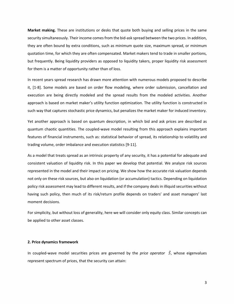
Market making. These are institutions or desks that quote both buying and selling prices in the same

security simultaneously. Their income comes from the bid-ask spread between the two prices. In addition,

they are often bound by extra conditions, such as minimum quote size, maximum spread, or minimum

quotation time, for which they are often compensated. Market makers tend to trade in smaller portions,

but frequently. Being liquidity providers as opposed to liquidity takers, proper liquidity risk assessment

for them is a matter of opportunity rather than of loss.

In recent years spread research has drawn more attention with numerous models proposed to describe

it, [1-8]. Some models are based on order flow modeling, where order submission, cancellation and

execution are being directly modeled and the spread results from the modeled activities. Another

approach is based on market maker’s utility function optimization. The utility function is constructed in

such way that captures stochastic price dynamics, but penalizes the market maker for induced inventory.

Yet another approach is based on quantum description, in which bid and ask prices are described as

quantum chaotic quantities. The coupled-wave model resulting from this approach explains important

features of financial instruments, such as: statistical behavior of spread, its relationship to volatility and

trading volume, order imbalance and execution statistics [9-11].

As a model that treats spread as an intrinsic property of any security, it has a potential for adequate and

consistent valuation of liquidity risk. In this paper we develop that potential. We analyze risk sources

represented in the model and their impact on pricing. We show how the accurate risk valuation depends

not only on these risk sources, but also on liquidation (or accumulation) tactics. Depending on liquidation

policy risk assessment may lead to different results, and if the company deals in illiquid securities without

having such policy, then much of its risk/return profile depends on traders’ and asset managers’ last

moment decisions.

For simplicity, but without loss of generality, here we will consider only equity class. Similar concepts can

be applied to other asset classes.

2. Price dynamics framework

In coupled-wave model securities prices are governed by the price operator �̂�, whose eigenvalues

represent spectrum of prices, that the security can attain:

4

�̂�𝜓𝑛 = 𝑠𝑛𝜓𝑛 (1)

Eigenvector elements 𝜓𝑛 are related to probabilities of attaining the price corresponding to the 𝑛-th state:

𝑝𝑛 = |𝜓𝑛|2 (2)

Obviously, price operator �̂� must be Hermitian since price is a real number. Price fluctuations, so typical

for financial markets are included by letting the price operator’s matrix elements fluctuate:

�̂�(𝑡 + 𝛿𝑡) = �̂�(𝑡) + 𝛿�̂�(𝑡) (3)

Let us now consider a model, in which the stock has only two states: one with price equal to bid price, and

the other with price equal to ask price.

𝜓 = (𝜓𝑎𝑠𝑘𝜓𝑏𝑖𝑑

) (4)

Writing Eq. (1) in matrix form we have:

(𝑠11 𝑠12𝑠12∗ 𝑠22

) (𝜓𝑎𝑠𝑘𝜓𝑏𝑖𝑑

) = 𝑠𝑎𝑠𝑘/𝑏𝑖𝑑 (𝜓𝑎𝑠𝑘𝜓𝑏𝑖𝑑

) (5)

Eigenvalues 𝑠𝑎𝑠𝑘 and 𝑠𝑏𝑖𝑑 are then expressed through matrix elements as

𝑠𝑎𝑠𝑘 =𝑠11 + 𝑠222

+ √(𝑠11 − 𝑠222

)2

+ |𝑠12|2 (6a)

𝑠𝑏𝑖𝑑 =𝑠11 + 𝑠222

− √(𝑠11 − 𝑠222

)2

+ |𝑠12|2 (6b)

These equations can be rewritten as

𝑠𝑎𝑠𝑘 = 𝑠𝑚𝑖𝑑 +Δ

2 𝑎𝑛𝑑 𝑠𝑏𝑖𝑑 = 𝑠𝑚𝑖𝑑 −

Δ

2 (7)

to represent the bid and ask prices spaced by the spread

Δ = √(𝑠11 − 𝑠22)2 + 4|𝑠12|

2 (8)

and around the mid price

5

𝑠𝑚𝑖𝑑 =𝑠11 + 𝑠222

=𝑠𝑏𝑖𝑑 + 𝑠𝑎𝑠𝑘

2 (9)

Classical model with single price without spread is produced by the following form of price operator:

�̂� = (𝑠 00 𝑠

) (10)

Let us write the fluctuating matrix elements 𝑠𝑖𝑘 in the following form:

𝑠11(𝑡 + 𝑑𝑡) = 𝑠𝑙𝑎𝑠𝑡(𝑡) + 𝑠𝑙𝑎𝑠𝑡(𝑡) 𝜎𝑑𝑧 +

𝜉

2 (11a)

𝑠22(𝑡 + 𝑑𝑡) = 𝑠𝑙𝑎𝑠𝑡(𝑡) + 𝑠𝑙𝑎𝑠𝑡(𝑡) 𝜎𝑑𝑧 −

𝜉

2 (11b)

𝑠12(𝑡 + 𝑑𝑡) =𝜅

2 (11c)

Here 𝑑𝑧 ∼ 𝑁(0,1), 𝜉~𝑁(𝜉0, 𝜉1) and 𝜅 is a complex number with |𝜅|~𝑁(𝜅0, 𝜅1). In such setup mid-price

and spread are given by equations

𝑠𝑚𝑖𝑑(𝑡 + 𝑑𝑡) = 𝑠𝑙𝑎𝑠𝑡(𝑡) + 𝑠𝑙𝑎𝑠𝑡(𝑡) 𝜎𝑑𝑧 (12a)

Δ = √𝜉2 + |𝜅|2 (12b)

Last price is then chosen from the 𝑠𝑏𝑖𝑑 and 𝑠𝑎𝑠𝑘 pair according to probability of their occurrence:

𝑠𝑙𝑎𝑠𝑡(𝑡 + 𝑑𝑡) = [𝑠𝑏𝑖𝑑 with probability |𝜓𝑏𝑖𝑑|

2

𝑠𝑎𝑠𝑘 with probability |𝜓𝑎𝑠𝑘|2 (13)

This setup includes the traditional Wiener process as a trivial case. Indeed, when 𝜉 = 𝜅 = 0 spread equals

zero, and

𝑠𝑙𝑎𝑠𝑡(𝑡 + 𝑑𝑡) = 𝑠𝑚𝑖𝑑(𝑡 + 𝑑𝑡) = 𝑠𝑙𝑎𝑠𝑡(𝑡) + 𝑠𝑙𝑎𝑠𝑡(𝑡) 𝜎𝑑𝑧 (14)

Typical price dynamics produced by the coupled-wave model is shown in Fig. 1.

6

Fig. 1. Typical price dynamics produced by the coupled-wave model.

3. Risk components

Given the price dynamics, we can now calculate risk as the amount of potential loss over a time horizon 𝑇.

Coupled-wave model contains three risk sources of different nature. Let us describe them separately.

Diffusion risk

This is the most familiar component arising due to diffusion of price with time. In equation Eq. (12a) it is

described by the component 𝑠𝜎𝑑𝑧, and is common to liquid and illiquid securities alike1. Over time

diffusion risk accumulates and prevails over spread. It can be quantified with Value-at-Risk (VaR) as:

𝐷𝑖𝑓𝑓𝑢𝑠𝑖𝑜𝑛 𝑉𝑎𝑅 = 1.65𝜎√𝑇 (15)

Parameter 𝜎 should not be confused for volatility. This parameter is related to the increments between

last price and the next period’s mid-price, as opposed to increments between last price and the next

1 Research shows that 𝜎 is related to spread [11]. However, in this model they are treated as independent quantities.

8

10

12

14

16

18

0 50 100 150 200 250

time

bid ask

7

period’s last price, which are used to calculate volatility. However, volatility can be expressed through 𝜎

and average spread ⟨Δ⟩ as

𝑉𝑜𝑙𝑎𝑡𝑖𝑙𝑖𝑡𝑦 = √𝜎2 + 𝑎⟨Δ⟩2 (16)

where coefficient 𝑎 depends on the type of probability distribution of the last price within spread.

Spread uncertainty risk

Spread is essentially the price that has to be paid if one wanted to close a small position immediately.

Spread may increase as a result of liquidity loss (low trading volume) as well as in volatile times (high

trading volume), amplifying potential losses [11], and this uncertainty is the second risk factor. Described

by Eq. (12b) that uncertainty comes from the random nature of parameters 𝜉 and 𝜅. Typical probability

distributions of spread along with their fits 𝑝(Δ) calibrated with coupled-wave model are shown in Fig. 2.

Some securities have very low 𝜉, in which case 𝑝(Δ) reduces to noncentral chi distribution, whose

analytical form is easy to fit.

Fig. 2. Probability distributions of spread and their calibrated fits on March 16, 2016.

Spread uncertainty risk can be quantified similarly to VaR using the 𝛼-quantile of its probability

distribution:

0%

10%

20%

30%

40%

p(spread) p(Δ)

IRBT𝜉1= 0.11 𝜅0 = 0.10 𝜅1= 0.05

0%

20%

40%

60%

p(spread) p(Δ)

LULU𝜉1= 0.0 𝜅0 = 0.04 𝜅1= 0.02

8

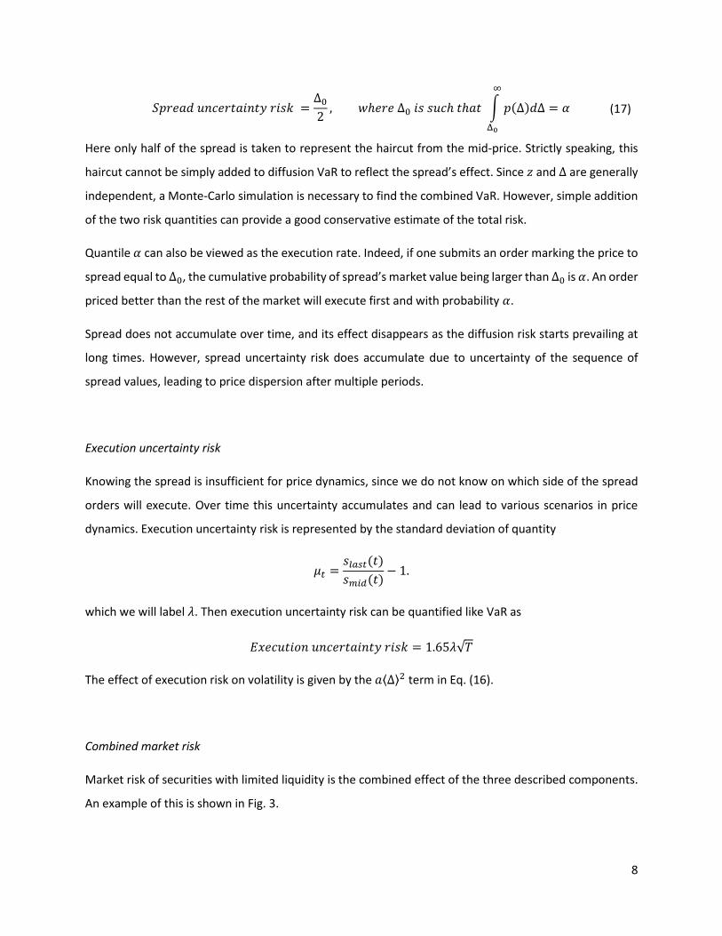
𝑆𝑝𝑟𝑒𝑎𝑑 𝑢𝑛𝑐𝑒𝑟𝑡𝑎𝑖𝑛𝑡𝑦 𝑟𝑖𝑠𝑘 =Δ02, 𝑤ℎ𝑒𝑟𝑒 Δ0 𝑖𝑠 𝑠𝑢𝑐ℎ 𝑡ℎ𝑎𝑡 ∫ 𝑝(Δ)𝑑Δ

∞

Δ0

= 𝛼 (17)

Here only half of the spread is taken to represent the haircut from the mid-price. Strictly speaking, this

haircut cannot be simply added to diffusion VaR to reflect the spread’s effect. Since 𝑧 and Δ are generally

independent, a Monte-Carlo simulation is necessary to find the combined VaR. However, simple addition

of the two risk quantities can provide a good conservative estimate of the total risk.

Quantile 𝛼 can also be viewed as the execution rate. Indeed, if one submits an order marking the price to

spread equal to Δ0, the cumulative probability of spread’s market value being larger than Δ0 is 𝛼. An order

priced better than the rest of the market will execute first and with probability 𝛼.

Spread does not accumulate over time, and its effect disappears as the diffusion risk starts prevailing at

long times. However, spread uncertainty risk does accumulate due to uncertainty of the sequence of

spread values, leading to price dispersion after multiple periods.

Execution uncertainty risk

Knowing the spread is insufficient for price dynamics, since we do not know on which side of the spread

orders will execute. Over time this uncertainty accumulates and can lead to various scenarios in price

dynamics. Execution uncertainty risk is represented by the standard deviation of quantity

𝜇𝑡 =𝑠𝑙𝑎𝑠𝑡(𝑡)

𝑠𝑚𝑖𝑑(𝑡)− 1.

which we will label 𝜆. Then execution uncertainty risk can be quantified like VaR as

𝐸𝑥𝑒𝑐𝑢𝑡𝑖𝑜𝑛 𝑢𝑛𝑐𝑒𝑟𝑡𝑎𝑖𝑛𝑡𝑦 𝑟𝑖𝑠𝑘 = 1.65𝜆√𝑇

The effect of execution risk on volatility is given by the 𝑎⟨Δ⟩2 term in Eq. (16).

Combined market risk

Market risk of securities with limited liquidity is the combined effect of the three described components.

An example of this is shown in Fig. 3.

9

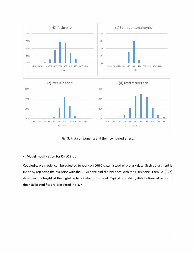
Fig. 3. Risk components and their combined effect.

4. Model modification for OHLC input

Coupled-wave model can be adjusted to work on OHLC data instead of bid-ask data. Such adjustment is

made by replacing the ask price with the HIGH price and the bid price with the LOW price. Then Eq. (12b)

describes the height of the high-low bars instead of spread. Typical probability distributions of bars and

their calibrated fits are presented in Fig. 4.

0%

10%

20%

30%

40%

-20% -16% -12% -8% -4% 0% 4% 8% 12% 16% 20%

return

(a) Diffusion risk

0%

20%

40%

60%

80%

-20% -16% -12% -8% -4% 0% 4% 8% 12% 16% 20%

return

(b) Spread uncertainty risk

0%

20%

40%

60%

-20% -16% -12% -8% -4% 0% 4% 8% 12% 16% 20%

return

(c) Execution risk

0%

10%

20%

30%

-20% -16% -12% -8% -4% 0% 4% 8% 12% 16% 20%

return

(d) Total market risk

10

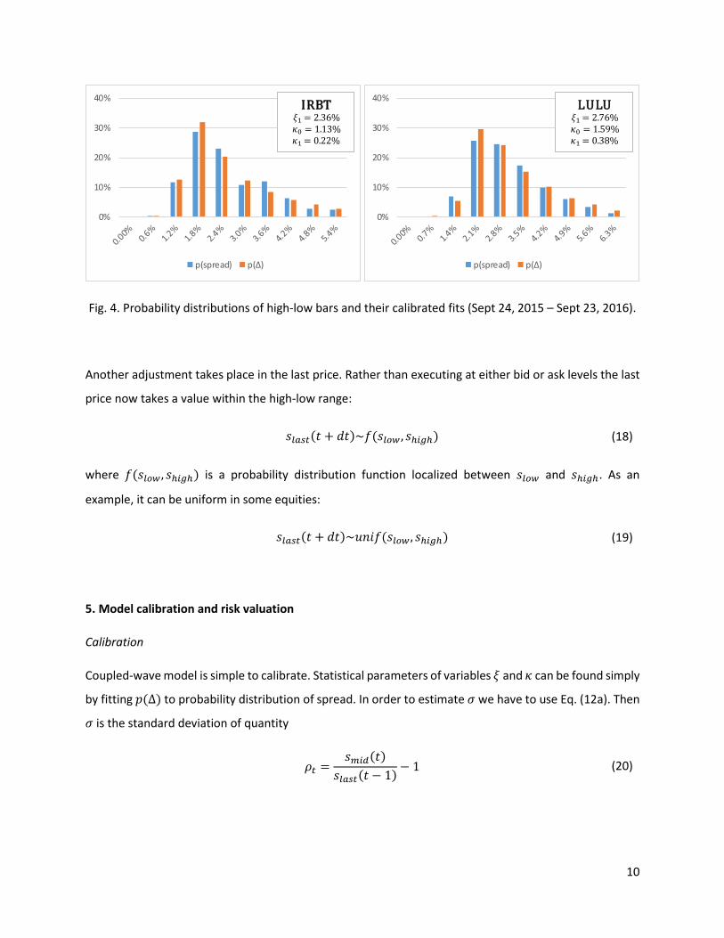
Fig. 4. Probability distributions of high-low bars and their calibrated fits (Sept 24, 2015 – Sept 23, 2016).

Another adjustment takes place in the last price. Rather than executing at either bid or ask levels the last

price now takes a value within the high-low range:

𝑠𝑙𝑎𝑠𝑡(𝑡 + 𝑑𝑡)~𝑓(𝑠𝑙𝑜𝑤 , 𝑠ℎ𝑖𝑔ℎ) (18)

where 𝑓(𝑠𝑙𝑜𝑤 , 𝑠ℎ𝑖𝑔ℎ) is a probability distribution function localized between 𝑠𝑙𝑜𝑤 and 𝑠ℎ𝑖𝑔ℎ. As an

example, it can be uniform in some equities:

𝑠𝑙𝑎𝑠𝑡(𝑡 + 𝑑𝑡)~𝑢𝑛𝑖𝑓(𝑠𝑙𝑜𝑤 , 𝑠ℎ𝑖𝑔ℎ) (19)

5. Model calibration and risk valuation

Calibration

Coupled-wave model is simple to calibrate. Statistical parameters of variables 𝜉 and 𝜅 can be found simply

by fitting 𝑝(Δ) to probability distribution of spread. In order to estimate 𝜎 we have to use Eq. (12a). Then

𝜎 is the standard deviation of quantity

𝜌𝑡 =𝑠𝑚𝑖𝑑(𝑡)

𝑠𝑙𝑎𝑠𝑡(𝑡 − 1)− 1 (20)

0%

10%

20%

30%

40%

p(spread) p(Δ)

IRBT𝜉1= 2. 6 𝜅0 = 1.1 𝜅1= 0.22

0%

10%

20%

30%

40%

p(spread) p(Δ)

LULU𝜉1= 2. 6 𝜅0 = 1.5 𝜅1= 0.

11

Market risk valuation

Once the model is calibrated it is ready to be used for market risk estimation. However, the exact level of

risk also depends on position size. Liquidation of a small size long position, goes by the market prices, and

using 𝑠𝑙𝑎𝑠𝑡 is appropriate to determine total VaR. If the position is larger than liquidity available in a single

time step, various options exist. For example:

(a) We can start selling the asset as soon as liquidity becomes available and keep doing it until position is

liquidated. In that case we limit the diffusion risk, but pay the haircut each time. Time horizon for such

strategy can be estimated as Δ𝑇 =𝑉

𝐿, where 𝑉 is the position size and 𝐿 is the expected daily volume.

Expected volume can be estimated conservatively as the lowest percentile of the observed volume2.

For fast liquidation strategy price dynamics can be described by applying Eq. (12a) with execution at bid

level in each step after 𝑇:

𝑠𝑙𝑎𝑠𝑡(𝑇 + Δ𝑇) = 𝑠𝑏𝑖𝑑(𝑇 + Δ𝑇) = 𝑠𝑙𝑎𝑠𝑡(𝑇) + ∑ (𝑠𝑙𝑎𝑠𝑡(𝑡′) 𝜎𝑑𝑧𝑡′ −

Δ𝑡′+𝑑𝑡′

2)

𝑇+Δ𝑇

𝑡′=𝑇

(21)

Then risk of loss can be computed traditionally as the lowest percentile of the resulting prices.

(b) Another option is to sell the asset slowly avoiding to disturb the market. This strategy benefits from

better pricing, but carries the diffusion and execution risks. Risk of loss can be then obtained by

multiperiod propagation of price using Eqs. (12-13).

(c) Any combination of the first two strategies can also be a valid liquidation strategy. For example, it may

seem feasible to sell 25% of the position at the outset of liquidation, another 25% at the end of time

horizon, and gradually selling the other 50% in between.

In each case, risk value will be different. Ultimately, the exact risk valuation depends on company’s policy

with respect to liquidation. If no policy exists, risk managers can make adequate assumptions based on

the nature of the position.

2 Spread and volume are related [11]. For daily data that relationship is near linear, so when volume is low spread also

tends to be low. As a result, liquidation takes more time, but requires a smaller price haircut. In the other extreme,

when volume is large, liquidation proceeds faster, but requires a bigger haircut.

12

As liquidation proceeds, the position size shrinks reducing risk with it. This effect needs to be taken into

account in VaR calculation. If ℎ(𝑡) is the position size as a function of time, 𝑙(𝑡) is the VaR relative to the

position, and 𝐿(𝑡) is the absolute value of value at risk, then

𝐿(𝑇2) = 𝐿(𝑇1) + ∫ ℎ(𝑡) 𝑑𝑙(𝑡)

𝑇2

𝑇1

(22)

For gradual uniform position reduction ℎ(𝑡) = ℎ𝑇2−𝑡

𝑇2−𝑇1, 𝑇1 ≤ 𝑡 ≤ 𝑇2, where ℎ is the initial size.

Example

Let us use the described framework to estimate market risk for Hercules Capital Inc stock traded on NYSE

(ticker HTGC). This stock is a moderate liquidity asset with 264,000 shares traded daily on average, and

has market capitalization around $1 bln. Let us assume that we hold a position of 1 mln shares, and we

want to calculate market risk of that position at time horizon of 1 month (22 trading days). For simplicity

we will neglect any possibility of dividend distributions.

Calibrated parameters for daily high-low bars for the interval of Sep 21, 2015 to Sep 16, 2016 are given in

the Table 1.

Table. 1. Calibrated parameters of the model for HTGC.

𝝃𝟏 1.99%

𝜿𝟎 1.20%

𝜿𝟏 0.49%

𝝈 1.11%

The fast answer is that the 95%-confidence haircut for the stock equals 2.2%, and total value-at-risk with

the same confidence equals 9.6%. The complete answer must address the details of how we are planning

to liquidate the position if we had to. Results are summarized in Table. 2.

13

Table. 2. Liquidation strategy comparison.

Daily volume Days to liquidate VaR Extra days Shares/day % of daily flow

Low liquidity 152,637 7 14.0% 61 16,393 10.74%

High liquidity 614,602 2 11.3% 23 43,478 7.07%

If at the end of the 22-day holding period liquidity dries to 1-year 5% lowest levels, then we will need 7

days to liquidate the position using all available NYSE liquidity. In doing so we would incur the risk of 14.0%

loss (taking into account position reduction during liquidation), which is 4.4% higher than if we had a small

position, so cost of liquidity is 4.4%. However, we would run the same level of risk if we liquidated slowly,

within 61 days but at market prices. In order to do that, we need to sell 16,393 shares/day, which would

then represent only 10.74% of trading volume. Such amount would not disturb the price much3.

Similarly, if trading volume increased, we would need only 2 days for fast liquidation. Incurred VaR would

then be equal 11.3%, so cost of liquidity is 1.7%. However, incurred VaR would be the same if liquidation

proceeded slowly at a rate of 43,478 shares/day over 23 days. That is only 7.07% of trading volume.

Depending on company’s capabilities, such liquidation can be accomplished earlier than in 23 days, saving

the risk for the company.

Ultimately, risk valuation should address these details by including their effect on potential losses.

6. Discussion

A few remarks about the model are in order. Eigenvalue problem Eq. (1) has been formulated for price

operator. Theoretically, this allows negativity of prices. A more appropriate formulation would have been

for the logarithmic price, which would exclude possibility of negative prices and include price scaling. In

this paper we deliberately based our formulation on price to make ideas easier to grasp.

The form of matrix elements in Eqs. (11a-11c) was chosen to facilitate convenient description of market

data for equity asset class. We do not claim that this is the only possible choice. Other formats may exist,

and analysts can adjust the presented framework to better capture the properties of the instruments they

are working with.

3 These scenarios should not be confused for stress-tests. 1-year 5% lowest or highest volume levels are quite

realistic, and stress tests would involve scenarios lying outside of that range.

14

Random variables 𝑧, 𝜉, and 𝜅 are described in the model as independent. Correlations between them can

be easily adapted, if data shows signs of their presence. We also used volatility 𝜎 as an independent factor.

However, spread Δ is connected to volatility as well as to trading volume as shown in [11]. This means

that ultimately the entire model can be formulated using only parameters 𝜉 and 𝜅.

When we modelled fast liquidation of large positions we assumed that prices would drop to the bid or

low levels. After such sessions prices tend to partially restore to previous levels. This effect can be included

by adjusting probability distribution 𝑓(𝑠𝑙𝑜𝑤, 𝑠ℎ𝑖𝑔ℎ).

Summarizing, the presented framework allows to measure market risk of financial instruments with

limited liquidity in a consistent way. This model can be calibrated to various types of data, such as best

bid-and-ask, effective bid-ask, or even OHLC bars. Using this framework, companies can accurately

measure risk associated with spread, model liquidation process, estimate liquidation costs, calculate the

possible range for bid and ask prices at the end of time horizon, etc. All these capabilities are extremely

important when a trading desk’s risk-return profile depends substantially on spread.

In conclusion, I would like to take this opportunity to express regards to the 2009-2011 S&T team of

Otkritie Financial Corporation and particularly Olga Dudolina, with whom we worked closely on risk limit

approval in those years. That work helped me understand business processes and requirements of the

business line and had a great impact on this paper.

7. References

[1] R. Cont, S. Stoikov and R. Talreja, “A stochastic model for order book dynamics", Operations research,

58, 549-563, (2010)

[2] R. Cont and A. de Larrard, “Order book dynamics in liquid markets: limit theorems and diffusion

approximations”, preprint, (2012)

[3] T-W. Yang, L. Zhu, “A reduced-form model for level-1 limit order books”, arXiv:1508.07891v3 [q-fin.TR],

http://arxiv.org/abs/1508.07891, (2015)

[4] I.M. Toke, N. Yoshida, “Modelling intensities of order flows in a limit order book”, arXiv:1602.03944

[q-fin.ST], http://arxiv.org/abs/1602.03944, (2016)

[5] M. Avellaneda, S. Stoikov, “High-frequency trading in a limit order book”, Quantitative Finance 8(3),

15

217–224 (2008)

[6] O. Gueant, C.-A. Lehalle, and J. Fernandez-Tapia, “Dealing with the inventory risk: a solution to the

market making problem", Mathematics and Financial Economics, Volume 7, Issue 4, pp 477-507, (2013)

[7] A. B. Schmidt, “Financial Markets and Trading: An Introduction to Market Microstructure and Trading

Strategies” (Wiley Finance, 2011)

[8] M.D. Gould, M.A. Porter, S. Williams, M. McDonald, D.J. Fenn, S.D. Howison, “Limit order books”,

preprint, (2013).

[9] J. Sarkissian, Quantum Theory of Securities Price Formation in Financial Markets (April 13, 2016).

Available at SSRN: http://ssrn.com/abstract=2765298

[10] J. Sarkissian, “Coupled mode theory of stock price formation”, submitted to PRE, available at

arXiv:1312.4622v1 [q-fin.TR], (2013)

[11] J. Sarkissian, “Spread, Volatility, and Volume Relationship in Financial Markets and Market Maker's

Profit Optimization” (June 23, 2016). Available at SSRN: http://ssrn.com/abstract=2799798