1

  

 

Risk, Returns, and Optimal Holdings of Private Equity 

Andrew Ang 

Morten Sorensen 

December 2011 

I. Introduction 

Private equity (PE) investments are investments in privately‐held companies, 

trading directly between investors, not on organized exchanges. The investments 

can be direct equity investments into individual companies. More commonly, though, 

they are made through a PE fund organized as a limited partnership with the 

investor as a limited partner (LP) and the PE firm as the general partner (GP), 

overseeing and managing the investments in the individual companies. Depending 

on the type of companies they invest in, PE funds are typically classified as buyout 

(BO) funds, venture capital (VC) funds, mezzanine debt funds, or some other type 

specializing in other illiquid non‐listed investments.  Additionally, it is not 

uncommon for LPs to make co‐investments directly into the portfolio companies in 

parallel to the investments made through the PE fund. 

PE is often considered a distinct asset class, and it differs from typical liquid, public 

equity investments in several fundamental ways:  First, there is no active market for 

PE positions, making these investments illiquid and difficult to value.  Second, the 

investments are long‐term investments. PE funds typically have horizons of ten to 

thirteen years during which the invested capital cannot be redeemed.  Third, 

partnership agreements specifying the funds’ governance are complex documents, 

  2

typically specifying the GP’s compensation as a combination of regular fees 

(Management Fee), a profit share (Carried Interest), and other fees. 

This article surveys the academic research about the risks and returns of PE 

investing and the optimal holdings of PE in an investor’s portfolio. It should be 

noted that researchers have had very limited access to information about the nature 

and performance of PE investments, and that the research in this area is preliminary 

and often inconclusive. Research into many important aspects of these investments, 

such as the performance of PE in the recession, the secondary market for LP 

positions, and LPs’ co‐investments in deals, has only recently begun.  

Section II introduces two main problems that research has encountered in 

measuring PE risk and returns. The first problem is the statistical problem that 

arises because PE returns are only observed infrequently, typically with well‐

performing funds being overrepresented in the data. This makes it difficult to 

estimate standard measures of risk and return, such as alphas and betas. Even after 

addressing this problem, a second problem arises about how to best interpret the 

resulting estimates. Standard asset‐pricing models are derived under assumptions 

that are appropriate for traditional financial markets – with transparent, liquid, and 

low‐friction transactions.  These assumptions are problematic for PE investments, 

and the estimated alphas and betas may need to be adjusted to provide meaningful 

measures of risk and return in the PE context.  One way of interpreting the risks and 

returns of PE investments, especially for illiquidity risk, is for an investor to 

consider PE from an investor‐specific asset allocation context. 

Section III summarizes the existing literature on the optimal allocation of PE in 

portfolios consisting of public liquid public equity and illiquid PE.  A new generation 

of asset allocation models considers these issues as the first generation of asset 

allocation approaches assumed that assets can be rebalanced without cost at any 

time.  The literatures on asset allocation incorporating transactions costs, which are 

very high for PE investment, and search frictions, since counterparties are often 

  3

hard to find for transferring PE investments, lead to some stark recommendations 

on optimal holdings of illiquid PE assets. 

In Section IV, we survey the literature on PE contracts with a special emphasis on 

fees and opaqueness.  Most PE investments are made through intermediaries.  

Current PE investment vehicles cannot disentangle factor returns unique to the PE 

asset class from manager skill.  Furthermore, commonly used contracts may 

exacerbate, rather than alleviate agency issues.   

Finally, Section V concludes by summarizing our recommendations of best practices 

for institutional investors when assessing and benchmarking PE returns, allocating 

funds between PE and liquid markets, and setting limited partnership agreements. 

 

II. Private Equity Risk and Return 

II. A. Evaluating Private Equity Risk and Return 

To understand the problems of evaluating PE investments, and to fix notation and 

terminology, it is useful to start from the standard model of risk and return. For 

standard liquid financial assets, risk and return are often measured by the   and   

coefficients from a one‐factor linear regression (the Expected Return Regression), 

 

In this equation   is the expected return earned by the investor from period 

t‐1 to period t,   is the risk‐free rate over the period from t‐1 to t, and   is 

the return on the market portfolio. Specifically, the return earned on a financial 

asset from time t‐1 to t is defined as 

1 

  4

Here D(t) is the dividend (or any cash flow more generally) paid out at time t, and 

P(t) is the market price quoted at time t, immediately after the payment of the 

dividend.  

For standard traded assets, the Expected Return Regression is straightforward to 

estimate by regressing the asset’s observed returns on the market returns over the 

same period.  The one‐factor specification given above, which includes just the 

excess market return factor (MKT) in the bracket on the right‐hand side of the 

equation, can be extended to multifactor specifications by including more factors, 

typically the value factor (HML), the size factor (SMB), and possibly a momentum 

factor (UMD) in the spirit of Fama and French (1993). 

Under appropriate assumptions about investors’ preferences, such as CRRA or 

mean‐variance utility, and assumptions about the market environment, such as the 

absence of transaction costs, short‐sales constraints, and the ability of investors to 

continuously trade and rebalance, the CAPM model specifies that each asset’s 

expected return is given by the Expected Return Regression with an alpha equal to 

zero. This important result has several implications: It implies that the appropriate 

measure of risk is  , which measures the correlation between the return on the 

asset and return on the overall market (Systematic Risk). Furthermore, the 

Systematic Risk is the only type of risk that is priced in equilibrium. Idiosyncratic 

risk is not priced, because it can be diversified away by investors. The Expected 

Return Regression further implies that an asset’s expected return increases linearly 

in  . Finally, it implies that in equilibrium, without arbitrage,   should be zero. A 

positive   can then be interpreted as an abnormal positive return. 

Following this logic, the standard approach to evaluating risks and returns of 

financial assets proceeds in two steps: First,   and   are estimated using the 

Expected Return Regression. Second, invoking the CAPM model, the estimated   

coefficient is interpreted as the abnormal return, and the estimated   is interpreted 

as the risk. 

  5

For PE investments problems arise at both steps: First, privately held companies do 

not have market values, by definition, and hence the returns earned from investing 

in these companies are only observed infrequently, making it difficult to estimate 

the Expected Return Regression. Moreover, privately held companies with better 

performance tend to be overrepresented in the data, creating a sample selection 

problem that may lead to an upward bias in the estimated   and a downward bias in 

the  . Second, even after obtaining estimates of   and   for PE investments, it is not 

obvious that these coefficients can be interpreted as measures of risk and returns. 

The assumptions of liquid and transparent markets underlying the CAPM model are 

far from the realities of PE investing, and the estimated coefficients may have to be 

adjusted in various ways – e.g., to account for the cost of illiquidity, idiosyncratic 

risk, persistence, funding risk, etc. – to reflect the actual risks and returns faced by 

the LP investors.  

II. B. Estimating Alphas and Betas of PE Investments 

The lack of regularly quoted market prices for PE investments means that PE 

returns are only infrequently observed, making it difficult to estimate the Expected 

Return Regression directly. The academic literature has approached this problem 

using several alternative data sources, primarily data with performance and 

valuations of company‐level investments and data with fund‐level cash flows 

between LPs and GPs. The result and limitations of these approaches are discussed 

next.  

II. B. 1. Company‐Level Data 

Two primary studies using company‐level data are Cochrane (2005) and Korteweg 

and Sorensen (2010). Both studies focus on VC investments. There is no comparable 

study of buyout (BO) investments, primarily due to the lack of data with deal‐level 

cash‐flow information for buyout investments.  

  6

Following Cochrane (2005) and Kortweg and Sorensen (2010), there are two main 

advantages of estimating risk and return from company‐level data relative to 

studies using fund‐level data (discussed below): First, there are many more 

companies than funds, and companies have well‐defined industries and types 

(early‐stage, late‐stage, etc.), leading to greater statistical power and a more 

nuanced differentiation of the risks and returns across industries, investment types, 

and time periods. Second, returns are well defined. Absent intermediate payouts, 

company‐level data directly lead to the return earned over the life of the investment 

(specifically, P(t‐1) is the initial investment, D(t) is the subsequent realized cash 

flow, earned when the investment is exited, and P(t) is the market value after the 

exit, typically zero). 

Company‐level data have three main disadvantages: First, company‐level cash‐flows 

do not subtract management fees and carried interest paid by the LPs to the GPs, 

hence estimated risks and returns reflect the total (gross of fees) risks and returns 

of the investments, not those earned by an LP (which are net of fees). Inferring the 

returns after fees to LPs requires additional assumptions (see Metrick and Yasuda 

(2010)).  We comment further on investor fees in Section IV. Moreover, company‐

level data require continuous‐time specifications and must correct for selection bias, 

as discussed next. 

Continuous‐Time Specifications 

A technical complication with company‐level data is that the returns are measured 

over different lengths of time. The standard (discrete‐time) CAPM model, with non‐

zero alpha, does not compound (it defines all returns as one‐period returns, where a 

period may last for an arbitrary amount of time – a day, a month, a quarter, etc. – but 

all returns must be defined over periods of equal length). 

This is a standard problem in empirical finance, and it is typically addressed by 

using the continuous‐time version of the CAPM model, which does compound over 

time and hence can used to compare risks and returns of investments of different 

  7

durations. In the continuous‐time CAPM model, the Expected‐Return Regression is 

restated in log‐returns (Continuously Compounded Returns) as follows 

ln ln ln ln  

Consequently, Cochrane (2005) and Korteweg and Sorensen (2010) estimate the 

continuous‐time version of the model. One complication arises, however, because 

the intercept of the continuous‐time specification can no longer be interpreted as 

the abnormal arithmetic return, as in the standard discrete‐time version of the 

model. Instead, the abnormal return is calculated by adding one‐half times the 

square of the estimated volatility, as follows 

. 

Volatility, however, is very high as Cochrane (2005) and Kortweg and Sorensen 

(2011) point out, and the arithmetic alphas calculated using this adjustment become 

correspondingly high. For example, Cochrane (2005) reports an annual volatility 

around 90%, resulting in an estimated alpha of 32% annually, which appears very 

high compared to studies using fund‐level data (see below). 

Selection Bias 

Studies using company‐level data face a sample‐selection problem. To illustrate, VC 

investments are structured over multiple rounds, and better‐performing companies 

tend to raise more rounds of financings. Hence, data sets with valuations of 

individual VC rounds are dominated by these better‐performing companies. 

Moreover, distressed companies are usually not formally liquidated, and are often 

left as shell companies without economic value (sometimes called “zombies”).  This 

introduces another selection problem for the empirical analysis. When observing 

old companies without new financing rounds or exits, these companies may be alive 

and doing well or they may be distressed zombies, in which case it is unclear when 

the write‐off of the company’s value should be recorded.  

  8

To illustrate the magnitude of the selection problem consider Figure 1 (from 

Korteweg and Sorensen (2010)).  The universe of returns is illustrated by all dots.  

The data, however, only contains the observed good returns above the x‐axis (drawn 

in black).  Worse returns (shaded in gray) are unobserved. Since only the black dots 

are observed in the data, a simple estimation of the Expected Return Regression 

gives an estimate of alpha that is biased upwards, an estimate of beta that is biased 

downwards, and a total volatility that is too low.  Hence, standard statistical analysis 

that does not correct for this selection bias will result in an overly optimistic view of 

the risk and return of these investments.  

Figure 1: Illustration of selection bias 

Models to account for such selection bias were first developed by Heckman (1979). 

Cochrane (2005) estimates the first selection model on VC data and finds that the 

effect of selection bias is indeed large.  The selection correction reduces the 

intercept of the log‐market model, denoted   above, from 92% to ‐7.1%. Cochrane 

also highlights the difficult of translating this intercept into an abnormal return. 

Korteweg and Sorensen (2010) estimate a more flexible and robust version of 

Cochrane’s model. They also find that selection over‐states the risk and return 

trade‐off of VC investments.  Without selection, the estimate of    is ‐0.0159 per 

month while taking into account the selection bias reduces this estimate to ‐0.0563 

per month.   

  9

In the continuous‐time model, the estimated   coefficient, without any adjustments, 

can still be interpreted as a measure of the systematic risk in the CAPM model. 

Cochrane finds a slope of 0.6‐1.9 for the systematic risk. This figure seems low, 

however, since it includes estimates at the individual industry levels of, for example, 

‐0.1 for retail investments. Korteweg and Sorensen (2010) report beta estimates 

that are substantially higher than those by Cochrane, in the range of 2.6‐2.8, which 

may be more reasonable for young startups funded by VC investors.   

Korteweg and Sorensen also find substantial variation over time. They estimate 

alphas over the periods 1987‐93, 1994‐2000, and 2001‐05, and find that the alphas 

in the early period were positive but modest, the alphas in the late 1990s were very 

high, but the alphas in the 2000s have been negative, consistent with patterns found 

by studies using fund‐level data.  

II. B. 2.  Advantages of Fund‐Level Data 

A recent survey by Harris, Jenkinson, and Kaplan (2011) summarizes the academic 

studies using fund‐level data from various data providers.1  There are several 

advantages to fund‐level data: First, fund‐level data reflect actual LP returns, net of 

fees, resulting in estimates of the risks and returns actually realized by the LPs. 

Additionally, the sample selection problem is smaller, since the performance of 

companies that ultimately never produce any returns for the investing funds 

(zombies) is eventually reflected in the fund‐level cash flows. Other sample selection 

problems may arise, however. Fund‐level performance is typically self‐reported, and 

better performing funds may be more likely to report their performance (as 

suggested by Phalippou and Gottschalg (2008), although Stucke (2011) finds that 

reported returns by Venture Economics have understated actual historical 

returns).2  Still, these selection problems are likely smaller than the more 

substantial problems that arise for company‐level data. Finally, since funds have 

                                                        1 These studies include Ljungqvist and Richardson (2003), Kaplan and Schoar (2005), Phalippou and Gottschalg (2008), and Robinson and Sensoy (2011).  2 Anecdotal evidence from Harris, Jenkinson, and Kaplan (2011) suggests that this bias made Venture Economics more attractive for benchmarking GP performance. 

  10

similar lifetimes (typically ten years), the Expected Return Equation can be 

estimated directly, avoiding the problems with the continuous‐time log‐return 

specification used for company‐level data.   

The main disadvantage of fund‐level data, however, is that it is unclear how to 

measure the "return." Absent quoted market prices, a stream of cash flows does not 

map into the definition of a return. Several alterantives have been proposed, but 

none of these are rooted in an economic valuation model and they all have various 

limitations, as discussed next. 

 

 II. C. Fund‐Performance Measures 

Fund‐level data typically contain a cash flow stream between the GP and LPs. Absent 

quoted market prices, these cash flows cannot be directly translated into returns. 

Calculating period‐by‐period returns requires assessing the market values of the PE 

investment (P(t) in the return calculation) at intermediate periods. Such market 

values are typically unavailable, and reported NAVs are noisy substitutes for these 

values (for example, it has been customary to value investments in individual 

companies at cost until the company experienced a material change in the 

circumstances, which clearly does not capture smaller ongoing changes in the 

prospects and market values of these companies). Given the absence of regularly 

quoted returns, several alternative measures have been proposed. However, none of 

these measures define a return, as defined in the CAPM model, and their 

relationships to standard asset pricing models are somewhat tenuous.  

II. C. 1. Internal Rate of Return (IRR) 

A natural starting point is to interpret the internal rate of return (IRR) of the cash 

flows between the LP and GP as a return earned over the life of the fund. Denoting 

the cash flow at time t as CF(t), and separating those into the capital calls paid by the 

  11

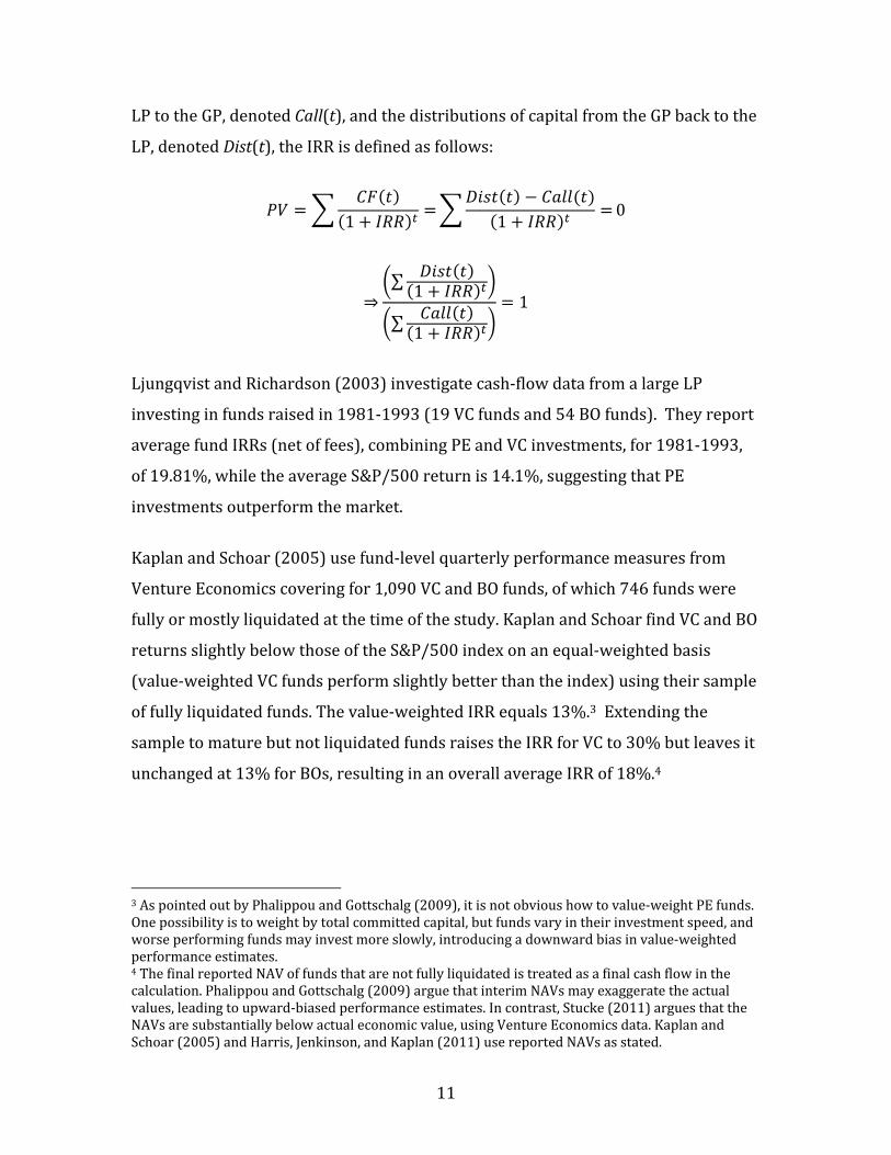
LP to the GP, denoted Call(t), and the distributions of capital from the GP back to the 

LP, denoted Dist(t), the IRR is defined as follows: 

1 10 

⇒∑

1

∑1

1 

Ljungqvist and Richardson (2003) investigate cash‐flow data from a large LP 

investing in funds raised in 1981‐1993 (19 VC funds and 54 BO funds).  They report 

average fund IRRs (net of fees), combining PE and VC investments, for 1981‐1993, 

of 19.81%, while the average S&P/500 return is 14.1%, suggesting that PE 

investments outperform the market.  

Kaplan and Schoar (2005) use fund‐level quarterly performance measures from 

Venture Economics covering for 1,090 VC and BO funds, of which 746 funds were 

fully or mostly liquidated at the time of the study. Kaplan and Schoar find VC and BO 

returns slightly below those of the S&P/500 index on an equal‐weighted basis 

(value‐weighted VC funds perform slightly better than the index) using their sample 

of fully liquidated funds. The value‐weighted IRR equals 13%.3  Extending the 

sample to mature but not liquidated funds raises the IRR for VC to 30% but leaves it 

unchanged at 13% for BOs, resulting in an overall average IRR of 18%.4  

                                                        3 As pointed out by Phalippou and Gottschalg (2009), it is not obvious how to value‐weight PE funds. One possibility is to weight by total committed capital, but funds vary in their investment speed, and worse performing funds may invest more slowly, introducing a downward bias in value‐weighted performance estimates.  4 The final reported NAV of funds that are not fully liquidated is treated as a final cash flow in the calculation. Phalippou and Gottschalg (2009) argue that interim NAVs may exaggerate the actual values, leading to upward‐biased performance estimates. In contrast, Stucke (2011) argues that the NAVs are substantially below actual economic value, using Venture Economics data. Kaplan and Schoar (2005) and Harris, Jenkinson, and Kaplan (2011) use reported NAVs as stated.  

  12

Focusing on VC investments, Bygrave and Timmons (1992) find an average IRR of 

13.5% over 1974‐1989, and Gompers and Lerner (1997), using the investments of a 

single VC firm, report an IRR of 30.5% over 1972‐1997.   

The recent summary by Harris, Jenkinson, and Kaplan (2011) compares 

performance measures for different data sources. For BO funds, they report 

weighted average IRRs of 12.3‐16.9%. For VC funds, the weighted average IRRs are 

11.7‐19.3%. Across time periods, BO funds have had more stable performance, with 

weighted average IRRs of 15.1‐22.0% in the 1980s, 11.8‐19.3% in the 1990s, and 

5.8‐12.8% in the 2000s. VC fund performance has more volatile over time, with 

weighted average IRRs ranging from 8.6 to 18.7% in the 1980s, 22.9 to 38.6% in the 

1990s, and ‐4.9 to 1.6% in the 2000s.  

Overall these figures reveal substantial uncertainty about even this most basic 

performance measure across the various studies and data sources. Moreover, the 

IRR is a problematic measure of economic performance. The IRR calculation 

implicitly assumes that invested and returned capital can be reinvested at the IRR 

rate. This means that if a fund makes a small investment with a rapid large positive 

return, this single investment can largely define the IRR for the entire fund, 

regardless of the performance of subsequent investments.5 

II. C. 2. Total‐Value‐To‐Paid‐In Capital (TVPI) 

An alternative performance measure that is less susceptible to manipulation than 

the IRR is the total‐value‐to‐paid‐in capital (TVPI) multiple. This multiple is 

calculated as the total amount of capital returned to the LP investors (net of fees) 

divided by the total amount invested (including fees). This calculation is performed 

without adjusting for the time value of money. Whereas the IRR is calculated under 

the implicit assumption that capital can be reinvested at the IRR rate, the TVPI is 

calculated under the implicit assumption that the capital can be reinvested at a zero 

rate. Formally, the TVPI is defined as 

                                                        5 Phalippou (2011) suggests that GPs may actively manage their investments to inflate fund IRRs. 

  13

∑

∑ 

Harris, Jenkinson, and Kaplan (2011) report weighted average TVPIs of 1.76‐2.30 

for buyout investors, and 2.19‐2.46 for VCs. This multiple has varied substantially 

over time. For BO funds, the reported multiple was 2.72‐4.05 in the 1980s, 1.61‐2.07 

in the 1990s, and 1.29‐1.51 in the 2000s. For VC funds, the reported multiple was 

2.31‐2.58 in the 1980s, 3.13‐3.38 in the 1990s, and 1.06‐1.09 in the 2000s. In other 

words, recent VC funds have, on average, simply returned invested capital, albeit 

after a ten‐year investment period.  

II. C. 3. Public Market Equivalent (PME)  

Both IRR and TVPI measure absolute performance, but it is even important to also 

understand the performance relative to the general market, and the third measure, 

the public market equivalent (PME), is a relative performance measure. 

The PME is calculated as the ratio of the discounted value of the LP’s inflows divided 

by the discounted value of outflows, with the discounting performed using realized 

market returns.  

∑∏ 1

∑∏ 1

 

As noted by Kaplan and Schoar (2005), under the assumption that PE investments 

have the same risk as the general market (a beta equal to one), a PME greater than 

one is equivalent to a positive economic return for the LPs. While generally 

reasonable, this interpretation may still be misleading because the economic risk of 

distributions (the numerator in the PME) is likely substantially greater than the 

economic risk of capital calls (including management fees, which resemble a risk‐

free liability). Using a lower discount rate for capital calls would inflate the 

denominator and reduce the PME. Hence, more carefully accounting for these 

  14

different risks suggests that the PME (calculated the traditional way) may have to 

exceed one by some amount before LPs actually earn a positive economic return.6  

Kaplan and Schoar (2005) find average equal‐weighted PMEs of 0.96. Value‐

weighted, the VC PME is 1.21 and the BO one is 0.93. Moreover, they report that 

larger funds have higher PMEs, although when funds become very large 

performance declines. For BO funds those with higher sequence numbers have 

higher PMEs. Phalippou and Gottschalg (2008) use 852 funds to calculate a PME of 

1.01, although this figure decreases to 0.88 after various adjustments.  

Looking across databases, Harris, Jenkinson and Kaplan (2011) report weighted 

average PMEs of 1.16‐1.27 for BO funds, and 1.02‐1.45 for VC funds. BO PMEs have 

varied from 1.03‐1.11 in the 1980s, to 1.17‐1.34 in the 1990s, and 1.25‐1.29 in the 

2000s. For VC, the reported PMEs are 0.90‐1.08 in the 1980s, to 1.99‐2.12 in the 

1990s, and 0.84‐0.95 in the 2000s. Relative to the market, the 1990s were the VC 

decade, and the 2000s have been the BO decade. 

II. C. 4. Risk Measures 

In contrast to company‐level data, fund‐level are poorly suited for estimating the 

risk of PE investing. Few, if any, academic studies attempt to use fund‐level data to 

do so. Instead, Ljungqvist and Richardson (2003) estimate risk by assigning each 

portfolio company to one of 48 broad industry groups and use the corresponding 

average beta for publicly traded companies in the same industry. They report that 

the corresponding beta for publicly traded companies is 1.08 for buyouts and 1.12 

for venture capital investments. Note that these betas do not adjust for the higher 

(lower) leverage used for buyouts (venture capital) investments. Assigning betas, 

they find a 5‐6% premium, which they interpret as the illiquidity premium of 

venture capital investments.  

                                                        6 Additionally, as a technical point, the CAPM model prescribes that the discounting should be performed using expected returns, not realized returns as in the PME. Using the realized returns distorts the calculation (according to Jensen's inequality). The magnitude of this distortion is unclear, but most likely modest. 

  15

Kaplan and Schoar state that they “believe it is possible that the systematic risk of 

LBO funds exceeds 1 because these funds invest in highly levered companies.” They 

regress IRRs on S&P/500 returns, and find a coefficient of 1.23 for VC funds and 

0.41 for BO funds. A (levered) beta of 0.41 seems unreasonably low, however. 

Hence, based on the existing evidence from studies using fund‐level data, it seems 

too early for a precise assessment of how the risk of PE investing compares to the 

risk of investing in publicly traded equities even in terms of these most basic 

metrics.  

II. C. 5. Persistence and Predictability 

A PE firm typically raises a sequence of partially overlapping funds (a fund family). 

Kaplan and Schoar (2005), Phalippou and Gottschlag (2009), and several other 

studies find evidence of perforamnce persistence of these funds. Good performance 

of a previous fund predicts good performance of subsequent funds in the same fund 

family. This is interpreted as evidence that GPs vary in their skills and abilities to 

pick investments and manage the companies. Estimates suggest that a performance 

increase of 1.0% for a fund is associated with around 0.5% greater performance for 

the subsequent fund in the same family, measured either in terms of PME or IRR. 

For more distant funds, the persistence declines.  

PE performance can also be predicted by other PE firm or fund characteristics along 

with macro economic variables.  It has been suggested that greater fund size may be 

related to smaller returns. Though, Kaplan and Schoar (2005) and Harris, Jenkinson, 

and Kaplan (2011) find no relation between size and performance for BO funds. For 

venture capital funds, Harris, Jenkinson, and Kaplan (2011) report a positive 

relation between size and performance after controlling for vintage years.  

Due to data limitations, studies that document predictability in PE returns conduct 

statistical analysis in sample, rather than on an out‐of‐sample basis.  In Kaplan and 

Schoar, for example, PE funds in the “top quartile” do well, but these funds are 

  16

identified ex post.  Within a fund family, funds often have lifetimes of 10 years but 

overlap to some extent. In‐sample analysis uses the ultimate performance of a 

previous fund to predict the performance of a subsequent fund, even if this 

subsequent fund is raised before the ultimate performance of the previous funds is 

fully realized.  The studies employ various robustness checks, such as using 

intermediate NAVs instead of ultimate performance or using the performance of 

funds several generations ago to predict future performance to mitigate this 

concern. Still, some recent research, such as Hochberg, Ljungvist and Vissing‐

Jorgensen (2010) find weaker evidence of persistence using only information 

available when the new fund is raised. 

II. D. Summary 

Measuring PE risk and returns is difficult because of the infrequent observations of 

fund or company values and selection bias.  Studies using company‐level data which 

account for selection bias find high alphas for PE investments only during the late 

1990s, but negative alphas post‐2000.  The positive alpha estimates are hard to 

interpret in terms of arithmetic returns, however, because of very high volatility. 

Estimates of PE betas vary substantially, ranging as high as 3.6 for venture capital 

investments.   Studies using fund‐level data have fewer selection problems, but still 

suffer from the fact that no direct PE returns are observed.  Unlike standard return 

measures, fund‐level IRRs, TVPI, and PME measures can all be misleading and 

should be used with caution to infer PE performance.  In terms of raw performance, 

in the words of Harris, Jenkinson, and Kaplan (2011) "it seems likely that buyout 

funds have outperformed public markets in the 1980s, 1990s, and 2000s." However, 

due to the uncertainty about the risk of private equity investments, it is not yet 

possible to say whether this outperformance is sufficient to compensate investors 

for the risk of these investments and whether the investments outperform on a risk‐

adjusted basis. Finally, there is evidence of persistence of PE fund returns and some, 

albeit weaker and less consistent, evidence that characteristics like fund size and 

past capital raisings predict PE fund returns. 

  17

III. Asset Allocations to Private Equity 

Having discussed the measurement of PE returns, we now consider optimal 

allocations to PE.  This requires, of course, a suitable risk‐return trade‐off for PE 

investments as well as correlations of PE returns with other assets in the investor’s 

opportunity set.  As Section II points out, measuring these inputs for PE for use in an 

optimization problem requires special considerations.  We take as given these 

inputs and focus on the dimension of illiquidity risk of PE and how to incorporate 

illiquidity PE risk into an optimal asset allocation framework. There have been 

several approaches to handling illiquidity risk in asset allocation, all of which have 

relevance in dealing with PE allocation.   To put into context these contributions, we 

start with the case of asset allocation without frictions. 

III. A.  Frictionless Asset Allocation 

The seminal contributions of Merton (1969, 1971) and Samuelson (1969) 

characterize the optimal asset allocation of an investor with CRRA utility investing 

in a risk‐free asset (with constant risk‐free rate) and a set of risky assets.  The CRRA 

utility function with risk aversion  is given by 

   

CRRA utility is homogeneous of degree one, which means that exactly the same 

portfolio weights arise whether $10 million of wealth is being managed or $1 billion. 

This makes the utility function ideal for institutional asset management.  

Assume the risky assets are jointly log‐normally distributed.  Under the case of iid 

returns, the vector of optimal holdings, w, of the risky assets are given by 

   

1

( ) .1

WU W

11( ),fw r

  18

where  is the covariance matrix of the risky asset returns,  is the vector of 

expected returns of the risky assets, and rf is the risk‐free rate.   This is also the 

portfolio held by an investor with mean‐variance utility optimizing over a discrete, 

one‐period horizon.   

There are two key features of this solution that bear further comment.  First, the 

Merton‐Samuelson solution is a dynamic solution that involves continuous 

rebalancing.  That is, although the portfolio weights, w, are constant, the investor’s 

policy is always to continuously sell assets that have risen in value and to buy assets 

that have fallen in value in such a way as to maintain constant weights.  Clearly, the 

discrete nature of PE investment and the inability to trade it frequently mean that 

allocations to PE should not be done with the standard Merton model.   

Second, the cost of employing a non‐optimal strategy, for example, not holding a 

particular asset which should be held in an optimal portfolio, can be compared to 

the optimal strategy and the cost of holding the non‐optimal portfolio depends on 

the investor’s risk aversion.  That is, the cost of bearing non‐optimal weights is 

dependent on the investor’s risk preferences.  The costs are computed using utility 

certainty equivalents: the certainty equivalent cost is how much an investor must be 

compensated in dollars per initial wealth to take a non‐optimal strategy but have 

the same utility as the optimal strategy.  A relevant cost, which the subsequent 

literature explores, is how much an investor should be compensated for the inability 

to trade assets like PE for certain periods of time or to be compensated for being 

forced to pay a cost whenever an asset is traded.   

III. B.  Asset Allocation with Transactions Costs 

Investing in PE incurs large transactions costs in initially finding an appropriate PE 

manager and conducting appropriate due diligence.  Then, there are potentially 

large discounts to the recorded asset values that may be taken in transferring 

ownership of a PE stake in illiquid secondary markets.  Since Constantinides (1986), 

a large literature has extended the Merton setup to incorporate transactions costs.   

  19

Constantinides considers the case of one risk‐free and one risky asset.  When there 

are proportional transactions costs, so that whenever the holdings of the risky asset 

increase (or decrease) by v, the holding of the riskless asset decreases by (1+k)v.  

When there are trading costs, the investor now trades infrequently.  Constantinides 

shows that the optimal trading strategy is to trade whenever the risky asset position 

hits upper and lower bounds,   and  , respectively. These bounds straddle the 

optimal Merton solution where there are no frictions.  The holdings of risky to risk‐

free assets, y/x, satisfy 

   

so that when y/x lies within the interval  there is no trade and when y/x hits 

the boundaries on either side, the investor buys and sells appropriate amounts of 

the risky asset to bring the portfolio back to the Merton solution. 

The no‐trade interval,  , increases with the transactions costs, k, and the 

volatility of the risky asset.  Transactions costs to sell PE portfolios in secondary 

markets can be extremely steep.  When Harvard endowment tried to sell its PE 

investments in 2008, potential buyers were requiring discounts to book value of 

more than 50%.7  Even for transactions costs of 10%, Constantinides computes no‐

trade intervals greater than 0.25 around an optimal holding of 0.26 for a risky asset 

with a volatility of 35% per annum.  Thus, PE investors should expect to rebalance 

PE holdings very infrequently.   

The certainty equivalent cost to holding a risky asset with large transactions costs is 

small for modest transactions costs, at approximately 0.2% for proportional 

transactions costs of 1%, but can be substantial for large transactions costs—which 

is the more relevant range of transactions costs for PE investments.  For 

                                                        7 See “Liquidating Harvard” Columbia CaseWorks ID#100312, 2010. 

w w

,y

w wx

[ , ]w w

w w

  20

transactions costs of 15% or more, the required premium to bring the investor to 

the same level of utility as the frictionless Merton case is more than 5% per annum.    

The literature has extended this framework to multiple assets (see, for example, Liu 

(2004)) and different types of rebalancing bands.  Leland (1996) and Donohue and 

Yip (2003) suggest rebalancing to the edge of a band rather than to a target within a 

band.  Others, like Pliska and Suzuki (2004) and Brown, Ozik, and Scholtz (2007) 

advocate extensions to two sets of bands, where different forms of trading are done 

at the inner band with more drastic rebalancing done at the outer band.  In all these 

extensions, the intuition is the same: PE investments should be expected to be 

rebalanced very infrequently, and the rebalancing bands will be very wide.  The case 

of transactions costs when returns are predictable is considered by Garleanu and 

Pedersen (2010).  A related study is Longstaff (2001), who allows investors to trade 

continuously, but only with bounded variation so there are upper and lower bounds 

on the number of shares which can be traded every period.  This makes Longstaff’s 

model similar to a time‐varying transactions cost. 

A major shortcoming of this literature is that it assumes that trade in assets is 

always possible, albeit at a cost.  This is not true for PE—over a short horizon, there 

may be no opportunity to find a buyer and even if a buyer is found, there is not 

enough time, relative to the investor’s desired short horizon to raise capital, to go 

through legal and accounting procedures to transfer ownership.   An important 

friction for PE investors in secondary markets is the search process in finding an 

appropriate buyer.  There may be no opportunity to trade, even if desired, at 

considerable discounts.  This case is what the next literature considers.  

III. C.  Asset Allocation with Search Frictions 

As PE investments do not trade on a centralized exchange, an important part of 

rebalancing a PE portfolio is finding a counterparty in over‐the‐counter markets.  Or, 

if money is spun off from existing PE investments, new or existing PE funds must be 

found to invest in. This entails a search process, incurring opportunity and search 

  21

costs, as well as a bargaining process, which reflects investors’ needs for immediate 

trade.  The latter is captured by a transactions cost, as modeled in the previous 

section.  The former requires a trading process that captures the discrete nature of 

trading opportunities.   

Since Diamond (1982), search‐based frictions have been modeled by Poisson arrival 

processes.  Agents find counterparties with an intensity , and conditional on the 

arrival of the Poisson process, agents can trade and rebalance.  This produces 

intervals where no rebalancing is possible for illiquid assets and the times when 

rebalancing are possible are stochastic.  This notion of illiquidity is that there are 

times where it is not possible to trade, at any price, an illiquid asset.  These 

particular types of stochastic rebalancing opportunities are attractive for modeling 

PE in another way: the exit in PE vehicles is often uncertain.  Although a PE vehicle 

may have a stated horizon, say of 10 years, the return of cash from the underlying 

deals may cause large amounts of capital to be returned before the stated horizon, 

or in many cases the horizon is extended to maximize profitability of the underlying 

investments (or to maximize the collection of fees by GPs). 

 A number of authors have used this search technology to consider the impact of 

illiquidity (search) frictions in various over‐the‐counter markets, such as Duffie, 

Garleanu and Pedersen (2005, 2009).  While these are important advances for 

showing the effect of illiquidity risk on asset prices, they are less useful for deriving 

asset allocation advice on optimal PE holdings.  Duffie, Garleanu and Pedersen 

(2005, 2009) consider only risk‐neutral and CARA utility cases and restrict asset 

holdings to be 0 or 1.  Garleanu (2009) and Lagos and Rocheteau (2009) allow for 

unrestricted portfolio choice, but Garleanu considers only CARA utility and Lagos 

and Rocheteau focus on showing the existence of equilibrium with search frictions 

rather than on any practical calibrations.  Neither study considers asset allocation 

with both liquid and illiquid assets.   

III. D.  Asset Allocation with Stochastic Non‐Traded Periods 

  22

Ang, Papanikolaou, and Westerfield (2011) [APW] solve an asset allocation problem 

with liquid securities, corresponding to traded equity markets which can be traded 

at any time, and illiquid securities, which can be interpreted as a PE portfolio.  The 

investor has CRRA utility with an infinite horizon and can only trade the illiquid 

security when a liquidity event occurs, which is the arrival of a Poisson process with 

intensity .  In this framework, the special case of Merton with continuous 

rebalancing is given by  .  As  decreases to zero, the opportunities to 

rebalance the illiquid asset become more and more infrequent.  The mean time 

between rebalancing opportunities is 1/.  Thus,  indexes a range of illiquidity 

outcomes.  

The inability to trade for stochastic periods introduces a new source of risk that the 

investor cannot hedge.  This illiquidity risk induces large effects on optimal 

allocation relative to the Merton case.  APW show that illiquidity risk affects the mix 

of liquid and illiquid securities even when the liquid and illiquid returns are 

uncorrelated and the investor has log utility.   

The most important result that APW derive is that the presence of illiquidity risk 

induces time‐varying, endogenous risk aversion.  The intuition is that there are two 

levels of wealth that are relevant for the investor: total wealth, which is the same 

effect as the standard Merton problem where the risk is that if total wealth goes to 

zero the agent cannot consume, and liquid wealth.  The agent can only consume out 

of liquid wealth.  Thus, with illiquid and liquid assets, the investor also cares about 

the risk of liquid wealth going to zero.  This can be interpreted as a solvency 

condition: an agent could be wealthy but if this wealth is tied up all in illiquid assets, 

the agent cannot consume.  Although the CRRA agent has constant relative risk 

aversion, the effective risk aversion—the local curvature of how the agent trades off 

liquid and illiquid risk in her portfolio—is affected by the solvency ratio of the ratio 

of liquid to illiquid wealth.  This solvency ratio also becomes a state variable that 

determines optimal asset allocation and consumption.  This illiquidity risk causes 

  23

the optimal holdings of even the liquid asset to be lower than the optimal holding of 

liquid assets in a pure Merton setting. 

APW derive five findings that are important considerations for investing in PE: 

1. Illiquidity risk induces marked reductions in the optimal holdings of assets 

compared to the Merton case.  Under APW’s calibrations for the same risk 

aversion as a 60% risky asset holding (and 40% risk‐free holding) in the 

Merton case, introducing an average rebalancing period of once a year 

reduces the risky asset holding to 37%.  When the average rebalancing 

period is once every five years, the optimal allocation is just 11%.  Thus, PE,  

which is highly illiquid, should be held in modest amounts (if at all) in 

investors’ portfolios. 

 

2. In the presence of infrequent trading, the fraction of wealth held in the 

illiquid asset can vary substantially and is very right skewed.  That is, 

suppose the optimal holding to illiquid assets is 0.2 when rebalancing can 

take place.  Then the investor should expect the range of illiquid holdings to 

vary from 0.15 to 0.35 during non‐rebalancing times. Because of the skew, 

the average holdings to the illiquid asset will be higher than the optimal 

rebalancing point, at say 0.25.  Thus, when an illiquid PE portfolio is 

rebalanced, the optimal rebalancing point is to a holding much lower than 

the average holding. 

 

3. The consumption policy (or payout policy) with illiquid assets must be lower 

than the Merton payout policy with only liquid assets.  Intuitively, holding 

illiquid assets means that there is additional solvency risk that liquid wealth 

goes to zero and consumption cannot be funded.   Thus, payouts of funds 

holding illiquid assets should be lower than the case when these assets all are 

fully traded.   

 

  24

4. The presence of illiquidity risk means that an investor will not fully take 

advantage of opportunities that might look like close to an “arbitrage”, for 

example, where correlations to the liquid and illiquid returns are nearly plus 

or minus one.  Traditional mean‐variance optimizers without constraints 

would produce weights close to plus or minus infinity in these two assets.  

This does not happen when one asset is illiquid because taking advantage of 

this apparent arbitrage involves a strategy that causes the investor’s liquid 

wealth to drop to zero with positive probability.  Thus, near‐arbitrage 

conditions when there is illiquidity risk are not exploited like the Merton 

setting.   

 5. Finally, the certainty equivalent reward required for bearing illiquidity risk is 

large.  APW report that when the liquid and illiquid returns are lowly 

correlated and the illiquid portfolio can be rebalanced, on average, once 

every five years (which is a typical turnover of many PE portfolios), the 

liquidity premium is over 4%.  For rebalancing once a year, on average, the 

illiquidity premium is approximately 1%.  These numbers can be used as 

hurdle rates for investors considering investing in PE.   

A number of authors including Dai, Li, and Liu (2008), Longstaff (2009), De Roon, 

Guo, and Ter Horst (2009), and Ang and Bollen (2010) also consider asset allocation 

where the illiquid asset cannot be traded over certain periods.  However, in these 

studies, the period of non‐trading is deterministic.  In contrast, the APW framework 

has stochastic and recurring periods of illiquidity.  Deterministic non‐trading 

periods are probably more appropriate for hedge fund investments where lock‐ups 

have known expirations.  PE investing is more open ended and has random, and 

infrequent, opportunities to rebalance.   

APW still miss a number of practical considerations that the future literature should 

address.  The most important one is that in the Merton setting into which APW 

introduce illiquidity, there are no cash distributions; all risky asset returns (both 

liquid and illiquid) are capital gains.  PE investments require cashflow management 

  25

of capital calls and distributions.  Some ad‐hoc simulations have been conducted by 

some industry analysts on this issue, like Siegel (2008) and Leibowitz and Bova 

(2009), but without explicitly solving optimal portfolios with illiquidity risk.  An 

extension of APW to incorporate cashflow streams could address this.   

III. E. Summary 

The inability to continuously rebalance PE positions, potentially even by paying 

transactions costs, makes optimal holdings of illiquid PE investments very different 

from the standard Merton framework which assumes no illiquidity risk.  Since 

transactions costs in rebalancing PE portfolios are very large, in both entering new 

PE positions and selling existing PE positions, PE positions should be expected to be 

rebalanced very infrequently and investors should set very wide rebalancing bands.  

In asset allocation models where illiquid assets like PE can only be traded upon the 

arrival of a (stochastically occurring) liquidity event, illiquidity risk markedly 

reduces the holdings of illiquid assets compared to the standard Merton model.  For 

example, an asset which could be traded continuously in the Merton setting that is 

held with a 60% optimal weight would have an optimal holding of less than 10% if it 

could be rebalanced only once every ten years, on average. The certainty equivalent 

reward, or equivalently the hurdle rate, for bearing illiquidity risk is large. For a 

typical PE investment that can be traded only once in ten years, on average, the 

illiquidity premium is well above 4%.  

 

IV. Intermediary Issues in Private Equity 

Most commonly, asset owners make PE investments as an LP in a fund where 

investment decisions are made by fund managers acting as GPs.  This arrangement 

raises potential agency issues.  One characteristic of PE investment is that the 

investment decisions arising from such management considerations and the related 

agency issues become intrinsically intertwined with PE performance. In public 

  26

equity markets, factor returns and active management can mostly be separated due 

to the existence of investable index strategies. 

While the agency problem is central for PE investments, there is only a small 

literature on optimal delegated portfolio management (see the good surveys by the 

BIS (2003) and Stracca (2006)).  There is, however, a large literature on agency 

issues in standard corporate finance settings (see, for example, the textbook by 

Salanie (1997) and Bolton and Dewatripont (2005)).  Delegated portfolio 

management is different from standard agency problems because the “action” 

chosen is generally observed (the investments made by the GP), but the set of 

actions is unknown (the full set of deals available to the GP).  In contrast, in standard 

moral hazard problems the “action” is unobservable, but the set of potential actions 

is usually known.8  Thus, little is known about the optimal delegated portfolio 

contract, and the literature has few, if any, specific conclusions or prescriptions 

about what form the optimal PE contract between LPs and GPs should take.   

PE investing is further complicated by having two levels of principal‐agent relations 

rather than just a single one: a level between the LPs (principal) and GPs (agent) 

and another level between the GPs as fund managers (principal) and its underlying 

portfolio of companies (agent). Both levels rely on strong direct monetary incentives. 

Apart from these monetary incentives, however, the relation between LPs and GPs is 

one with limited information, poor monitoring, rigid fee structures, and the inability 

to withdraw capital, or directly control managers. These features may exacerbate 

tensions between the LPs and GPs and exacerbate, rather than alleviate, agency 

issues.  On the other hand, the distance between the LP and GP may allow GPs to 

invest and manage companies more freely.  

                                                        8 There are other technical reasons that make the delegated optimal portfolio management problem challenging.  The agent (fund manager) can control the both the mean, which is the response to the signal by buying a good stock, but also the variance, through leverage.  In a typical agency problem the agent controls only the mean (occasionally the variance), but not both.  In continuous time, which is often used to solve agency problems, diffusion dynamics are effectively observable at high enough frequencies.   

  27

The other principal‐agent relation between the fund and its portfolio companies is 

one with strong governance, transparent information flows, good incentives for 

monitoring, and a high alignment of interests between owners and management 

(Jensen, 1989).  There is strong evidence that PE funds add significant value, on 

average, to the companies in their portfolio. This literature is surveyed by Kaplan 

and Stromberg (2009).  

The interactions between these two layers of principal‐agent problems have not 

been fully explored. It is not inconceivable, though, that mitigating the principal‐

agent problems at the LP‐GP level would come at the cost of increasing the problems 

at the fund‐company level. For example, greater transparency about the 

management of individual portfolio companies may in turn lead GPs to manage 

these companies with an eye towards managing short‐term earnings expectations 

and satisfying public expectations more broadly, a concern for publicly traded 

companies, rather than simply managing companies to maximize their total value.  

IV. B. Private Equity Contracts  

Because PE is, by its nature, private, it is difficult to perform systematic large‐sample 

studies of contractual features and see how they relate to performance. Gompers 

and Lerner (1999), Litvak (2009), and Metrick and Yasuda (2010) examine small 

samples of various PE contracts.  Several tentative conclusions emerge:  

1. PE contracts are largely standardized. An often‐quoted fee arrangement is a 

management fee of 2% and a carry of 20%.  There is some variation in the 

numbers (e.g., management fees tend to vary between 1‐2.5% and carried 

interest varies between 20‐35%), but the general structure is widely used. 

Additionally, a substantial part of the GPs compensation may be in the form 

of transaction fees.  PE fees are high. 

2. There is some variation in the specific provisions governing the calculation 

and timing of the fees and carried interest. For example, a management fee 

could be flat (on committed capital), declining over the life of the fund, a 

  28

(time‐varying but deterministic) combination of committed and managed 

capital, or even an absolute amount.   

3. Fixed fee and performance components are not substitutes but complements.  

That is, funds tend to raise both the fixed fee and variable fee components 

(and the other compensation components) together.  Fund size tends to 

positively correlated with fees, yet as Kaplan and Schoar (2005) and many 

others find, is negatively correlated with performance. Ignoring the 

endogeneity of fees and effort expended by the GP, these two facts imply that 

LPs are worse off in larger funds, which have both relatively poorer gross 

and net performance.  

4. There is a debate about the performance sensitivity of PE compensation. 

Metrick and Yasuda (2010) find that close to one‐half the present value of GP 

compensation are from management fees rather than carried interest and 

find this to be true for both VC and BO funds.  However, Chung et al. (2011) 

point out that a substantial amount of GPs' performance pay arises through 

the continuation value of raising future funds, which are highly sensitive to 

current performance.    

5. PE contracts are complex documents. Litvak (2009), however, finds little 

relation between opaqueness and total compensation.   

The management fees charged by private equity and venture capital funds are high. 

According to Metrick and Yasuda (2010) such fees consume at least one‐fifth of 

gross PE returns. Metrick and Yasuda found that out of every $100 invested with a 

VC fund, an average of $23 is paid to the GPs in the form of carry and management 

fees. For BOs, the mean of the carry and management fees comes to $18 per $100. 

The high fees charged by GPs point to the fact that if an institutional investor 

wishing to allocate to PE can do this in‐house, then there are substantial savings 

available.  Of course, attracting talent and running an in‐house PE shop presents a 

different set of agency issues than out‐sourcing to PE funds with GPs. Despite the 

pessimistic view of returns of PE investments to LPs in Section II, the high PE fees 

  29

implies that if asset owners can come close to capturing gross returns, PE becomes 

much more attractive.   

While opacity per se does not seem to be related to total compensation and returns, 

opacity has other important knock‐on effects for other aspects of an asset owner’s 

larger portfolio.  Complexity and non‐transparency can increase agency problems 

and make risk management more difficult. The leverage involved in many BO funds 

can be more expensive, and is often harder to monitor, than leverage done directly 

by the asset owner.    

 

V. Conclusions 

To summarize our findings and recommendations for PE investing: 

1. In measuring PE risk and returns, selection bias – the phenomenon that 

valuations, or company deals, tend to be observed only when underlying 

returns are good – is a major problem.  Naïve analysis without accounting for 

sample selection bias overstates average returns, understates risk measures 

like betas, and results in volatility estimates that are too low.  Studies taking 

into account sample selection reduce alpha, or average return, estimates by 

more than half.  Company‐level volatility estimates of PE returns are 

extremely high.   

Recommendation: For investors with current PE portfolios where company‐level 

data is available, measurement of PE returns must use econometric techniques to 

handle selection bias.  Investors should substantially adjust downwards expected 

return estimates and adjust upwards risk estimates of “raw” PE returns. 

2. The most commonly used fund‐performance measure, the IRR, is highly 

problematic and does not represent true underlying returns.  Even this most 

basic measure has substantial variation across various studies and data 

  30

sources.  Other fund‐level performance statistics show that since the 2000s, 

PE has not out‐performed public market equities and in many cases has 

significantly under‐performed. 

Recommendation: For PE investments post‐2000, expect performance in line or 

below that, on average, of public equity market returns.   

3. Models of asset allocation that take into account transactions costs, which are 

large for PE, and illiquidity risk, which is substantial for PE, recommend 

modest holdings of PE.  In these models, rebalancing will be infrequent, so 

wide swings in the holdings of PE should be expected, and the holdings of 

illiquid PE will be much lower than predicted by asset allocation models 

assuming that all assets can be rebalanced when desired. 

Recommendation: When determining optimal PE allocations, asset allocation 

models must take into account the inability to rebalance PE positions. There should 

be generally modest allocations to illiquid PE investments. 

4. Current PE vehicles have substantial agency issues which public equity 

vehicles do not.  While there is heterogeneity in PE contracts, PE fees are 

very large and consume at least one‐fifth of gross PE returns.  Incentive fees 

account for less than one‐third of GP compensation.   

Recommendation: If any of the fees paid to externally‐managed PE funds with GPs 

can be brought back in‐house to institutional asset owners, then if quality in PE 

investments can be maintained, there will be substantial savings to asset owners.  

 

 

  31

Bibliography 

Ang, Andrew and Nick Bollen (2010) "Locked Up by a Lockup: Valuing Liquidity as a Real Option," Financial Management, 39, 3, 1069‐1095 

Ang, Andrew, Dimitri Papanikolaou and Mark Westerfield (2011) "Portfoliio Choice with Illiquid Asset," working paper 

Bygrave, W., and J. Timmons (1992) “Venture Capital at the Crossroads” Harvard Business School Press, Boston 

Chen, Peng, Gary T. Baierl, and Paul D. Kaplan (2002) “Venture capital and its role in strategic asset allocation,” Journal of Portfolio Management, 28, 83‐90 

Chung, Ji‐Woong, Berk A. Sensoy, Lea H. Stern, Michael Weisbach (2011) "Pay for Performance from Future Fund flows: The Case of Private Equity," forthcoming Review of Financial Studies 

Cochrane, John (2005) “The risk and return of venture capital,” Journal of Financial Economics, 75(6), 1671‐1720 

Constantinides (1986) "Capital Market Equilibrium with Transaction Costs", Journal of Political Economy, 94(4), 842‐62 

Dai, Li and Liu (2008) wp 

De Roon, Guo and Ter Horst (2009) wp  

Driessen, Joost, Tse‐Chun Lin, and Ludovic Phalippou (2011) “A New Method to Estimate Risk and Return of Non‐Traded Assets from Cash Flows: The Case of Private Equity Funds” forthcoming Journal of Financial and Quantitative Analysis. 

Garleanu (2009) "Pricing and Portfolio Choice in Illiquid Markets" Journal of Economic Theory, 144(2), 532‐564 

Gompers, Paul, and Joshua Lerner (1997) “Risk and reward in private equity investments: the challenge of performance assessment,” Journal of Private Equity, 5‐12 

Harris, Robert, Tim Jenkinson, and Steven N. Kaplan (2011) “Private Equity Performance: What Do We Know?” working paper  

  32

Hwang, Min, John M. Quigley, and Susan Woodward (2005) “An Index For Venture Capital, 1987‐2003,” Contributions to Economic Analysis & Policy, 4(1), 1180–1180. 

Jones, Charles and Matt Rhodes‐Kropf (2003) “The Price of Diversifiable Risk in Venture Capital and Private Equity,” Working Paper. 

Kaplan, Steven N. and Antoinette Schoar (2005) “Private Equity Performance: Returns, Persistence, and Capital Flows,” Journal of Finance, 60 (4). 

Korteweg, Arthur and Morten Sorensen (2010) “Risk and Return Characteristics of Venture Capital‐Backed Entrepreneurial Companies,” Review of Financial Studies, 23(10), 3738‐3772. 

Ljungqvist, Alexander and Matthew Richardson (2003) “The Cash Flow, Return and Risk Characteristics of Private Equity” working paper. 

Lo, Mamaysky and Wang (2004) "Asset Prices and Trading Volume under fixed Transactions Costs," Journal of Political Economy, 112(5), 1054‐1090 

Longstaff (2009) forthcoming AER 

Metrick, Andrew and Ayako Yasuda (2010) "The Economics of Private Equity Funds," Review of Financial Studies, 23, 2303‐2341 

Metrick, Andrew and Ayako Yasuda (2010) "Venture Capital and Other Private Equity: A Survey," working paper 

Peng, Liang (2001) “Building A Venture Capital Index,” Working Paper 

Phalippou, Ludovic (2009) "Beware when venturing into private equity," Journal of Economic Perspectives 

Phalippou, Ludovic and Oliver Gottschalg (2009) "The performance of private equity funds," Review of Financial Studies, 22(4), 1747‐1776 

Quigley, John, and Susan Woodward (2002) “Private equity before the crash: Estimation of an index,” working paper 

Vayanos (1998) "Transaction Costs and Asset Prices: A Dynamic Equilibrium Model," Review of Financial Studies, 11, 1‐58