risk required return
TRANSCRIPT
8/8/2019 Risk Required Return
http://slidepdf.com/reader/full/risk-required-return 1/19
R I S K A N D T H E R E Q U I R E D R E T U R N O N E Q U I T Y
F R E D D . A R D I T T I *
FO R AN INVESTMENT to be acceptable to a firm's financial management it mustprovide a positive answer to the question "Will the acquisition of this assetincrease the value of the owner's equity?" If the investment meets this require-ment, then by definition the present value of the investment exceeds its cost.Conversely, in order for a firm's management to choose only those investmentswhich meet this maximization of equity value criterion, they must choose only
those investments whose present value to the owners exceeds the costs ofinvestment. However to determine the capitalized value of an asset the firm'sfinancial management must be able to estimate the cash flows which willaccrue and be distributed to the stockholders from the investment and therate at which these flows are capitalized by the market. To identify thiscapitalization rate or required return on equity and its relation to various typesof investment risks is the aim of this study.
A model which identifies several risk variables and their relationship to therequired rate of return is presented in Section I. The risk variables are divided
into two groups: (a) those that are directly associated with the probabilitydistribution of returns of a firm's stock, such as the second and third momentsof the distribution and the coefficient of correlation between the returns froma single stock and all other available stocks; and (b) those variables whichare intertwined with the firm's financial policies—the dividend-earnings andthe debt-equity ratios. Un der the assumption tha t the stock ma rket receivedwhat it expected over the 1946-1963 period, the actual return for each stockin the S ta n d a r d s P oor's Composite Index (industrials, railroads, and utili t ies)is used as a measure of the required return and regressed on the afore-
mentioned risk variables. The results are presented in Section II. Section IIIcontains a summary of the results and some conclusions that can be drawnfrom them.
I . T H E M O D E L
The principle of expected utility maximization enables the specification of
certain types of investor risks. Let the investor's wealth be denoted by W
and his income by the random variable X. Fu rtherm ore, let his utility function,
U, be solely dependent on the sum of his wealth and income. That is,
U = U(X + W) (1)Define a new random variable r = X /W , where r may be interpreted as the

8/8/2019 Risk Required Return
http://slidepdf.com/reader/full/risk-required-return 2/19
20 The Journal o f Finance
Expanding U in a Taylor series about w + E ( r W ), wbere E (r W ) repre-
sents the expected value of income, taking the expected value of both sides, and
assuming that W and E(r W) are constant, gives
E ( U) := :U[W + E ( r W ) ] + — ^ U " ( W + W f i i) n2 (2)
-| U"'(W -f- W Hi) li3 + terms involving higher order movements
where i^i, 1x2, and M3̂ denote the first, second, and third moments of r's probability
distribution. Equation (2) states that the expected utility is a function of
those risks associated with the higher moments of a probability distribution.
Note that attention has been concentrated on the second and third momentsof r's distribution. This has been done because the higher moments of r add
little, if an y, information abo ut the d istribution's phy sical features.^
The above relationship has been derived without making any assumptions
about tbe investor's attitude towards risk taking. This must now be done to
arrive at a testable hypothesis concerning the variability and skewness^ of
returns as risk measures and the relation of such measures to the required or
expected return. Assume that the typical investor is risk averse. Economic
theory describes the risk averter as one whose marginal utility or wealth
decreases with increasing wealth. That is,
U"(W ) < 0 (3)
Condition (3) states that the coefficient of H2 mu st be negative. T h e economicimplication of this negative sign is direct— the greater the v ariability of retu rnof an investm ent, the lower the expected utility of the investm ent. Con sequentlyfor the investment to retain its appeal under an increase in the variability ofreturns and no change in the other moments, its expected return must increase.
One implication of the diminisbing marginal utility assumption is tbat tbe
cash equivalent of the expected utility is less than the expected utility of tbeventure. This proposition is true for any concave utility function. The amountby which the expected value exceeds the cash equivalent of the expectedutility is called tbe risk premium. It can be tbought of as the amount theinvestor must be given in order for him to risk a sum equal to his cashequivalent. Using Pratt 's approach, it is possible to define the risk premiumma thematically.* Le t o^ be th e varian ce of income and n: a me asu re of thelocal risk premium. Then
o^jnw),2 U'(W)
8/8/2019 Risk Required Return
http://slidepdf.com/reader/full/risk-required-return 3/19
Risk and the Required Return on Equity 21
Now it can be argued that the investor attaches a smaller risk premiumto any given risk the greater his wealth. For example, consider the situationwhere two individuals, one poor and the other extremely wealthy, each find
themselves in possession of a ticket which entitles the holder to partake in thefollowing game:
"If on one flip of the coin a head appears the ticket holder receives $20,000.On the other hand, if a tail appears, the holder must pay $10,000." Who woulddemand a higher price for the sale of his ticket?
It seems reasonable to assume that the wealthy man would since a loss of$10,000 to him would be trivial while a similar loss to the poor man wouldrender him assetless. But the price the seller is willing to accept is the cashequivalent of his expected utility, and the difference between the cash equivalent
and expected value of the ticket is by definition the risk premium. Since theasking price of the wealthy man is higher than that of the poor man and eachticket has the same expected value, the wealthy individual's risk premium isless than tha t of the poor ma n's. Therefore one m ay infer th at the risk prem iumdecreases with wealth.
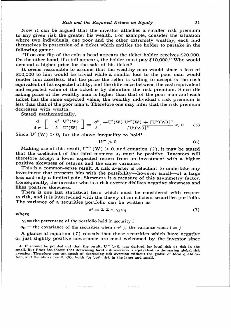
Stated mathematically,
g^ U^^(W) "I _ ^ -U ^(W ) U^^ (̂W) + [U "(W )] "
dw L 2 U'(W) J ~ T [
Since U' (W) > 0, for the above inequality to hold*
U '" > 0 (6)
Making use of this result, U'" (W) > 0, and equation (2), it may be statedtha t th e coefficient of th e third mom ent H3 must b e positive. Inv esto rs w illtherefore accept a lower expected return from an investment with a higherpositive skewness of returns and the same variance.
This is a common-sense result. A risk averter is reluctant to undertake anyinvestment that presents him with the possibility—however small—of a large
loss and only a limited gain. Skewness is a measure of th is asym m etry factor.Consequently, the investor who is a risk averter dislikes negative skewness andlikes positive skewness.
There is one last statistical term which must be considered with respectto risk, and it is intertwined with the theory of an efficient securities portfolio.The variance of a securities portfolio can be written as
0^ =z S 2 Yi Yj Oij (7)
where
Yi = the percentage of the portfolio held in security iOij = the covariance of the securities when i 7^ j ; the variance when i := j

8/8/2019 Risk Required Return
http://slidepdf.com/reader/full/risk-required-return 4/19
22 The Journal of Finance
they tend to reduce the over-all variance of the portfolio. Another way ofsaying the same thing is that those stocks whose returns are found to benegatively correlated with the other securities available to the investor are
desired since
where
rij = the correlation coefficient between the returns of the i*"" and j " " securities
01 = the standard deviation of the rate of return of the i*" security
In short, because they tend to reduce the over-all riskiness of the portfolio,the investor likes stocks that are n egatively correlated w ith the average m arke tmovements and he requires a lower rate of return from such securities.
Up to now the discussion has centered on those risk variables which stemfrom the firm's distribution of returns. We now turn to consider that other setof risk variables—those associated with the firm's financial policy. The setconsists of the firm's debt and dividend policies. Each is considered in turn.
The greater the proportion of debt in the firm's capital structure the morelikely it is that shareholders will lose everything or strike it rich. In otherwords, the greater the firm's leverage the higher the variability of the earningsavailable for distribution to shareholders. Thus the risk of debt is that it in-creases the variance of returns. The firm's debt-equity ratio can be taken as
a measure of this. Consequently, as the firm's debt-equity ratio increases, therisk borne by the shareholder increases and the expected utility of the invest-ment decreases. The only way in which the investment can retain its appealto the shareholder is for the expected utility of the investment to increase orat least remain constant. However for this to occur, the expected or requiredreturn from the investment must increase.
The effect of a firm's dividend policy on the capitalization rate of its equityhas been the subject of innumerable studies. These studies have been directedto the question of whether the market is willing to pay a premium for the
stock of a company which pays out a high proportion of its earnings.In search of an answer, two basic theories have been put forward. The
first which we dub the "dividends-do-count" theory holds that an increase inthe dividend payout is accompanied by a decrease in the required return.Proponents of this theory reason in the following manner. Since the variabilityof dividends is less than the variability of stock prices, any substitution ofdividends for capital gains in the over-all return received by the shareholderwill reduce the variability of this return. This reduction in risk induces a re-duction in the required return. The other school of thought is that dividends
have no affect on the capitalization rate. This theory is best articulated in theMiller-Modigliani article, "Dividend Policy, Growth, and the Valuation of

8/8/2019 Risk Required Return
http://slidepdf.com/reader/full/risk-required-return 5/19
Risk and the Required Return on Equity 23
dividends. This, in effect, increases the present cash flow or dividend streamrelative to the capital gains stream and therefore reduces the over-all vari-ability of returns. To those who contend that brokerage fees might prevent
the shareholder from following this course of action Miller and Modiglianireply that there might be just as many, if not more, people who are accumu-lators rather than dissavers and for them having topay the brokerage fee in
order to reinvest their dividends causes them to dislike a high dividend payout.
In any event both schools of thought on the relationship of the dividend-
earnings ratio to the required return agree that the differential between the
personal income and capital gains taxes works in favor of a preference for
low dividend payout. One gets the distinct impression from the l i terature that
the "dividends-do-count" supporters believe that the uncertainty or variability
effect outweighs the tax differential effect; so that the required return willdecrease with the dividend-earnings ratio. In direct contrast, Miller and
Modigliani feel that if dividends have any effect on the required return it will
occur via the tax differential effect and therefore the required return should
increase with the dividend-earnings ratio.
To recapitulate, the model as it now stands is.
p = ao + aiXi -f a2X2 + 33X3 + 34X4 -f-
where p, Xi, X2, X3, X4, and X5 denote respectively the required return, vari-ance, skewness, correlation coefficient between the stock's return and all
others which might comprise the shareholder's portfolio, debt-equity ratio, and
the dividend earnings ratio. The signs of the coefficients are expected to be
ai > 0; a3 < 0; ag > 0; a4 > 0; as ?
II. THE SPECIFICATION AND T E S T OF THE M O D E L
In order to test a model empirically the required return must be defined
specifically to enable it to be measured. The specific definition which shall beused rests on the assumption that inthe long run investors receive what theyexpect. That is the actual and required rates are one and the same. Thenassuming that all dividends are reinvested in the stock, the actual return can
be calculated as that rate of return which equates an investment of Po in one
nhare to an investment in IX (1 - j - Dt/Pt) shares each valued at Pndollars.t=-i
That is.
8/8/2019 Risk Required Return
http://slidepdf.com/reader/full/risk-required-return 6/19
24 The Journal of Finance
the solution of (8) is equivalent to the geometric mean of annual rates of
return.'̂
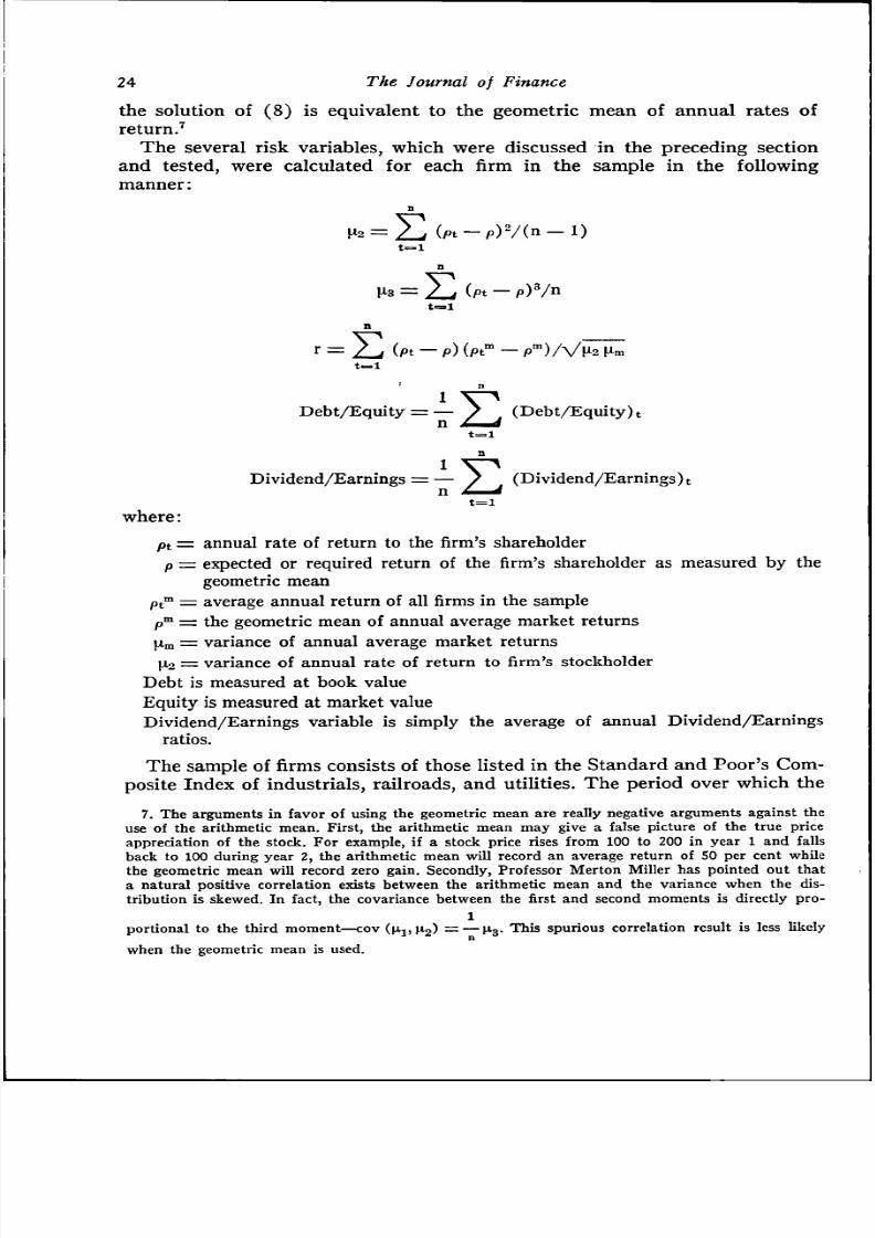
The several risk variables, which were discussed in the preceding section
and tested, were calculated for each firm in the sample in the followingmanner:
t = i
t=i
\
Debt/Equity = — / (Debt/Equity)tn LmmA
t = l
Dividend/Earnings = — / (Dividend/Earnings) tn JL^
t=i
w h e r e :
pt ^ annual rate of return to the firm's shareholder
p = expected or required return of the firm's shareholder as measured by the
geometric mean
pt™ = average annual return of all firms in the sample
p " ^ the geometric mean of annual average market returns
(Xm = variance of annual average market returns
[i2 = variance of annual rate of return to firm's stockholderDebt is measured at book value
Equity is measured at market value
Dividend/Earnings variable is simply the average of annual Dividend/Earnings
ratios.
Th e s a mp le of firms consists of those l is ted in the S t a n d a r d and P o o r ' s Com-
pos i te Index of indus t r ia l s , r a i l roads , and ut i l i t ies . The per iod over which the
7. The arguments in favor of using the geometric mean are really negative arguments against the
use of the arithmetic mean. First, the arithmetic mean may give a false picture of the true priceappreciation of the stock. For example, if a stock price rises from 100 to 200 in year 1 and fallback to 100 during year 2, the arithmetic mean will record an average return of SO per cent while
8/8/2019 Risk Required Return
http://slidepdf.com/reader/full/risk-required-return 7/19
Risk and the Required Re turn on Equity 25
study extends is 1946-1963. It will be apparent that the sample size varies indifferent regressions. The reason for this is that a firm is dropped from thesample if the data available for that firm are considered inadequate for anadequate estimate to be made of the variables involved. The inadequacycriterion is the following: if less than thirteen consecutive years of data areavailable for the calculations the firm is eliminated. Because several firmsfailed to meet this requirement the full contingent of S&P's firms never appearsin any regression.
The model is tested in the following manner. First the required return isregressed on only those variables termed distribution variables—tbe variance,skewness, and market correlation of a firm's returns. Then in a separate set ofregressions the financial variables—debt/equity and dividend/earnings—are
run against the required return. Finally, all the risk of variables are broughttogether in a set of regressions on the required rate of return. This stepwisemethod of testing the model has been used so that a clear picture can bepresented of how the several risk variables individually and collectively affectthe required return and eacb other.
A. The Distribution Variables
The first regression is run across all firms regardless of industry classifica-
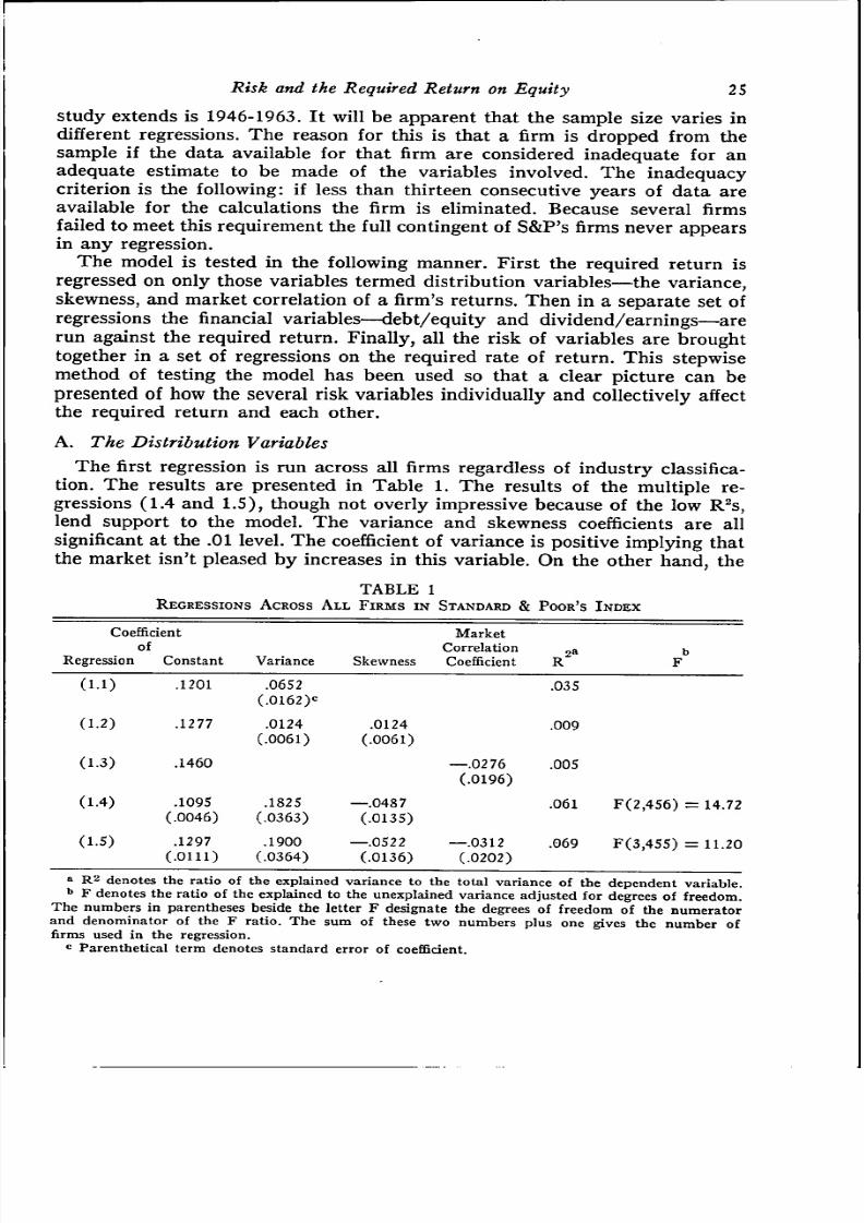
tion. T he results are presented in Tab le 1. T he results of the mu ltiple re -
gressions (1.4 and l.S), though not overly impressive because of the low R^s,lend support to the model. The variance and skewness coefficients are all
significant at the .01 level. The coefficient of variance is positive implying that
the market isn't pleased by increases in this variable. On the other hand, the
TABLE 1REGRESSIONS ACROSS ALL FIRMS IN STANDARD & POOR'S INDEX
Coefficientof
Regression Constant
(1.1)
(1.2)
(1.3)
(1.4)
(1.5)
.1201
.1277
.1460
.1095
(.0046)
.1297(.0111)
Variance.0652
(.O162)<=
.0124(.0061)
.1825
(.0363)
.1900(.0364)
Skewness
.0124(.0061)
—.0487
(.0135)
—.0522
(.0136)
MarketCorrelation
Coefficient
—.0276
(.0196)
—.0312(.0202)
.035
.009
.005
.061
.069
b
F
F(2,456) = 14.72
F(3,455) = 11.20

8/8/2019 Risk Required Return
http://slidepdf.com/reader/full/risk-required-return 8/19
26 The Journal of Finance
negative coefficient of the skewness variable means that the market likespositive skewness. The market correlation coefficient is nowhere significant.®
In an effort to relieve the bias on the regression coefficients due to riskeffects peculiar to each industry, industry dummy variables were introduced.It was not computationally feasible to include dummies for all the industriesrepresented among the 400-odd firms. Therefore they were only included forthose industries which provided enough data for later intra-industry tests onthe various risk variables. Th ere were seven in all, and they consisted of retailstores, food prod ucers, oils, chemicals, aerospace, drugs , and m achinery. Reta ilstores was chosen as the dummy-less or basic industry.
The first two regression runs using this reduced sample are the same asthose run in the previous test. The dummies were not yet included. The resultsare startlingly better (see Table 2—equations 2.1 and 2.2). Although themarket correlation coefficient remains insignificant, the variance and skewnesscoefficients remain significant at the .01 level while the R^ more than doubles.An acceptable explanation of these results must await further analysis; how-ever, one can surmise that the improved R^ must in some way be due to theincreased homogeneity of the sample obtained by the elimination of all but
TABLE 2REGRESSIONS ACROSS ALL FIRMS IN SELECTED INDUSTRIES
Coefficientof
Regression Constant
(2.1)
(2.2)
(2.3)
(2.1)
(2.2)
(2.3)
.1044
(.0074)"
.1137
(.0157)
.1001
(.0200)
Chem.
—.0094(.0128)
Variance
.4221
(.0831)
.4195
(.0833)
.3965
(.0909)
Aero
.0252
(.0164)
Skewness
—.1677
(.0435)
—.1673
(.0435)
—.1641
(.0447)
Drugs
.0200
(.0146)
MarketCorrelationCoefficient
—.0152
(.0227)
.0030
(.0241)
Mach.
—.0057
(.0117)
R^"
.147
.150
.212
Oil
.0023
(.0137)
F
F(2 ,162)
F(3 ,161)
F(9,155)
Food
.0244
(.0138)
b
= 14.00
= 9.45
= 4.64
denotes the ratio of the explained variance to the total variance of the dependent variableb F denotes the ratio of the explained to the unexplained variance adjusted for degree of freedom

8/8/2019 Risk Required Return
http://slidepdf.com/reader/full/risk-required-return 9/19
Risk and the Required Return on Equity 27
seven industries. The third equation in Table 2 and the standard errors of itscoefficients indicate that the industry dummies are insignificant. The result is
a bit surprising, since the result expected was that there would be some riskspeculiar to each industry with the variability, skewness, and market correla-tion coefficient do not account for. The only ones that might be consideredsignificant at some very low level (.20) are the oil and aerospace dummies.This seems reasonable since they probably represent the riskiest industriesrelative to retail stores.
The next step in the analysis was to determine how the coefficients of thethree risk variables tested varied with the different industries. To this end, anindustry regression was run for each of the seven industries. The results are
presented in Table 3.In all but the food industry the variable coefficients proved insignificant.
The failure of these risk variables to prove significant when run in intra-industry regressions and their high significance in the regressions on all firmsirrespective of indu stry (see Tab les 1 and 2) leads one to believe th at it isinter-industry differences in variance and skewness which account for themajor portion of the explanatory power of these variables. An analysis of co-variance technique was used to test this hypothesis. In essence, the analysisconsisted of estimating the coefficients of the following equation by ordinary
least squares and then testing for their significance.
\ — p =
3 = 1 3 = 1
where
Pi), xij, and yij respectively denote the required return, variance, and skewness ofthe i"" firm in the j " " industry;
xj and yj are the average variance and skewness respectively of the j * " industry and
are mathematically defined in the following manner:
•" 3 ro j
r_ 1 V _ - 1
where
mj is the number of firms in the j * * " industry;
P, X, and y, are the average required return, variance, and skewness across all firmsin all industries. Mathematically,

8/8/2019 Risk Required Return
http://slidepdf.com/reader/full/risk-required-return 10/19
28 The Journal of Finance
j j O C
i So
oCJ
O J
i n
IICOCN
C N
C O
p
1—1 CN
1
CO CO
^ O
CO
• o
i n
11C N
C O
fa
v O V O
CO v nC> p
O t^^- 1 CNCN CN
t^ O
o ^-*O CO
3 o
CO
COv O
O
II•
N̂
C N
fa
CO
on
6 0
OO O N
in in
00 O
in rsO O
03CN
C O
0 0
11o
C O
fa
t o
o oO CO
6 6
OS 00
ir> lo
•^ -?lO CNO O
C N
CO
o
II0 0
C N
fa
o
00 -H
.0 .3
T—1 f V|
v O CN
CO
C O
0 0S O
11
. — <CO
fa
O
OS rt
p p
CO »n
.0 .4
Tj - \O ^
OO lO
so OCN C N
2 o
X I
CO
oC N
IICO
CN
fa
CN(N
in 00
.0 .1
• * COCN C NCNI CO
CO COO CN—1 O
a
CO
• o
IIC N
C O
fa
soCS
q
00 —<rt OSCV] t ^
C3 q
CN O
.0 .1
Tt - COCN CO
OS OSO -" I -
—> o
CO
81
II1—1
fa
so
q
.1 .1
ON COVO OCN r^CO CO
l o
CO
O S
CO
IIo
CO
fa
so
o
so r^00 OSOS .^r
c3 • - ;
rsi 00
.1 .1
0 0 COCN CO
OS ^
X I' O
CO
O S
- ^
IIT j -
'• i.C N
fa
inin1—1
CO " ?
.6 .41
o o
v OCO
T - l
IICO
CO
fa
in
OC O
i n CNON O N' ^ 0 0
r^ inv O C NVO C N
TJ - O N
O O
Xi
v OC O

8/8/2019 Risk Required Return
http://slidepdf.com/reader/full/risk-required-return 11/19
Risk and the Required Return on Equity 29
• «ti^
O C
-5g
- ; v O
CM' «
in
o -<
VO
O
O -H .-<VO O CTv— —1 CO
1 =
IIC 3
^ o
III
S S c
s = • ; !
§•5 2> ca
•^2 fe
c•a

8/8/2019 Risk Required Return
http://slidepdf.com/reader/full/risk-required-return 12/19
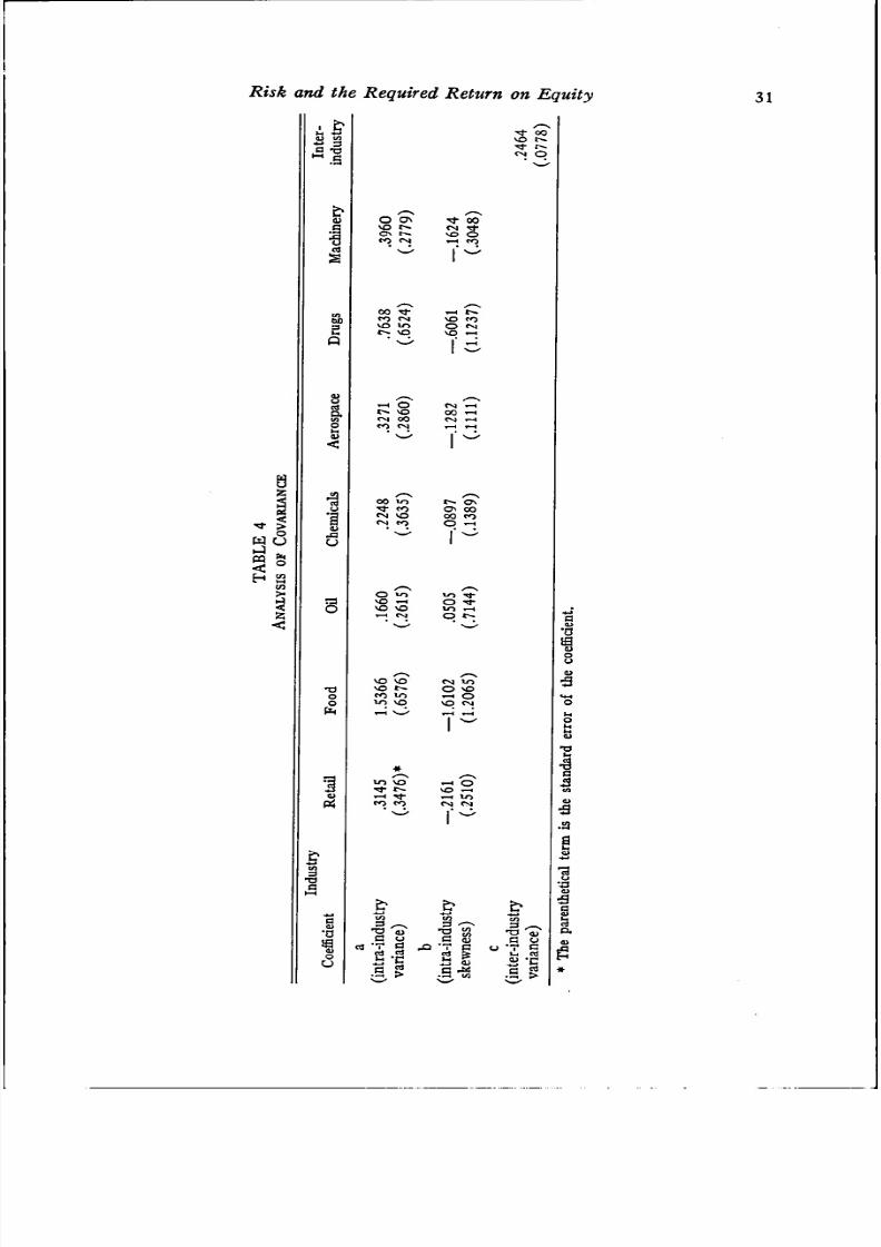
30 The Journal of Finance
The aj's and bj's represent the various intra-industry effects of the independent
variables on the required return; c and d represent the inter-industry effects.
Ta ble 4 lists the values of th e various coefficients and their standard^ erro rs
prior to the introduction of th e inter-industry skewness variable (yj — y ) -
Except for the coefficient of variance in the food industry, all intra-industry
coefficients are statistically insignificant. On the other hand, the coefficient of
the variable which measures the effects of differences in industry variance,
(xj — x), is significant at tbe .01 level.
When the industry skewness variable is introduced into the regression
equation (result not shown), both inter-industry_variables are insignificant.
The fact that xj — x becomes insignificant when yj — y enters the equation
does not mean that industry variance and skewness difference^ have no effecton the required return. The insignificance of Xj— x and yj — y is attributable
to the purely statistical problem of multicollinearity rather than any economic
factor. The correlation between xj — x and yj — y is .962. In any case, the
evidence of all prior regressions coupled with the results presented in Table 4
provide strong support for the theory that to a great extent the explanatory
power of variance and skewness lies in their in du stry differences.
B . The Financial Variables
Of the several risk variables considered in this model, tbe only one on which
a significant amount of empirical research has been done is tbe dividend
payout. Therefore it seems appropriate to briefly review and comment upon
the work done by others on this variable and its relation to the required return
on equity.Most studies use the annual stock price as the dependent variable. This,
however, does not prevent one from drawing conclusions as to what theirresults would have been if the required rate of return had been used sincestock price and required return are inversely related. The first of these
inquiries was conducted by Graham and Dodd. They ran a regression of stockprice vs. dividends and retentions. From the fact that the dividend coefficientwas approximately three times the retention coefficient they concluded thatinvestors are willing to pay a two dollar premium per share for every dollarthat is shifted from retentions to dividends.* Succeeding studies conducted byHarkavy and Gordon supported these results." Unfortunately, though theresults of these various tests appear convincing, the tests are less than sound
To begin with, if any variable which is correlated with the dependentvariable is omitted from the regression, the coefficient of the independent
variable will be biased. For the two variable case, the bias factor is the producof the coefficient of the omitted variable in the true relation and the regression
8/8/2019 Risk Required Return
http://slidepdf.com/reader/full/risk-required-return 13/19
Risk and the Required Return on Equity 31
.s
VO
CM
O N t"*»CO rg
'^ 00eg ^NO Or-H C O
CO Tf T-H
CO eg vO
t ^CNCO
OVO00CN
CM00CN
00• < J -
CNCN
lOCOVOCO
t ^ON00
O
00CO
oVOO
•aoo
VO
vOCOin
VO
VO
VO
OO
O
O VO-H OVO CN
-H OVO -H

8/8/2019 Risk Required Return
http://slidepdf.com/reader/full/risk-required-return 14/19
32 The Journal of Finance
variable. For example, if the variance of returns is omitted from the re-
gression equation and firms behave so as to reduce their dividend-earnings
ratio when this variability increases while the market pays a lower price for
carrying this increase in variability, the bias will be positive.
The second point is concerned with the notion that the market has an
expected dividend-earnings ratio. If the price of the stock is at all related
to dividends it is related to this ratio. Because firms are quite concerned with
the stability of their dividend stream, annual dividends are a good measure of
expected dividends. The same cannot be said of annual earnings or retentions.
Random shocks to normal earnings make it highly improbable that earnings
in any single year will be equal to expected earnings. Annual earnings or re-
tentions will deviate from expected earnings or retentions by an error term.Consequently the use of annual dividends and retentions in the regression
equation will lead to a positive bias in the dividend's coefficient if dividends
and retentions are positively correlated. They are. For firms in the Standard
and Poor's Index the average correlation over 1946-1963 was .284. This bias
factor associated with the use of annual data may not arise when dividend and
earnings figures are average over a number of years, for it is much more
likely that this averaged data will represent the market's expectations with
respect to dividends and retentions.
The last point concerns the notion that there are times when managementdeems the stock to be overpriced (that is they expect the market's required
return to rise). At such times, management may forego using retentions to
finance investments in favor of a new stock issue. Consequently, the result
of this overpricing may be an increase in the dividend-payout. Similarly,
reasoning shows that when management believes the stock to be underpriced
it may take action which will lower the dividend-payout. What all this means
is that when models are tested over a time span short enough for a stock to
be realistically considered over- or underpriced, the testers must recognize
the simultaneous nature of the model." The empirical analysis follows.The first step in the financial variable analysis was to regress the debt-equity
and dividend-earnings ratios separately and then jointly on the required
return across all available firms without regard to industry groupings. The
results of these tests are presented in Table 5. The single variable regressions
(equations 5.1 and 5.2) show that the slope coefficient of the debt-equity ratio
is insignificant, while the dividend-earning s ratio is negatively and significantly
correlated (at the .05 level) with the required rate of return. When both
financial variables are brought together in a single regression the results are
unaltered.The implication of the negative dividend coefficient is that the market

8/8/2019 Risk Required Return
http://slidepdf.com/reader/full/risk-required-return 15/19
Risk and the Required Return on Equity 33
FINANCIAL
Coefficientof
VARIABLE
Constant
REGRESSIONS
DebtEquity
T A B L E 5
ACROSS AL L F IRM S
DividendEarnings
IN STANDARD
R ' "
& POOR'S INDEX
F
.1342 —.0078
( .0106) ' •»» '
7 S .0..
a R2 denotes the ratio of the explained variance to the total variance of the dependent variable.
*> F denotes the ratio of the explained to the unexplained variance adjusted for degrees of freedom.The num bers in parentheses beside the letter F designate the degrees of freedom of the nu meratorand denominator of the F ratio. The sum of these two numbers plus one gives the number of firmsused in the regression.<= Paren thetical term denotes standard erro r of coefficient.
The fall in the significance of the dividend/earnings variable when thedistribution variables are entered (see Table 6) can be attributed to its nega-tive correlation with the variance (— .15). If one were to apply a strict .05 testto the dividend/earnings coefficients of equations 6.2 and 6.3, the coefficientswould be insignificant and this would be accepted as evidence in favor of the
Modigliani-Miller theory. But they are too close to being significant to bequickly cast aside, so judgment must be deferred.
A strong positive correlation between variance and debt/equity results in astill more nega tive de bt /equ ity coefficient (see equations 6.2 and 6.3 ). Theonly explanation I can offer for the still negative—although insignificant—debt-equity ratio is that there are inter-firm risks which are not accounted forby the probability distribution variables. When these risks are high, the firmwill reduce its debt-equity ratio in an attempt to lower its riskiness while itsshareholders will demand a high return for holding the risky stock. If some of
these risks are indigenous to each industry grouping, then the true nature ofthe debt/equity-required return relationship will be disclosed by testing thisrelationship within industries. Furthermore, such a test will provide addedevidence on the dividend-required return theories.
The results of regressing the required return first on the financial variablesand then on all the risk variables of the model are presented in Table 7.Before the introduction of the distribution variables into the regressionequation, the coefficient of the dividend-earnings ratio is significant at the.05 level in three of the six industries—retail stores, foods, and chemicals."
After the distribution variables are introduced into the equation the dividend-earnings ratio becomes insignificant in all industries. However, the fact that

8/8/2019 Risk Required Return
http://slidepdf.com/reader/full/risk-required-return 16/19
The Journal of Finance
a
Mak
Coea
Dvdn
Db
•a
u
v
Sw
Enn
Ey
an
(^
in O
O -H
vO CNO O
Ov 00r^ Ov
O O
Tt- Ov 00 rsi^^ in lr> VOvO ^^ VO -H
O O O O
>O lO VO •«CM O «N) O
o o
OO ̂ Ov 5
So So
8 S
^ fOVO O
o o o o
1^ 1
ooo
fO Ov 1
^ 00 1
2 S

8/8/2019 Risk Required Return
http://slidepdf.com/reader/full/risk-required-return 17/19
Risk and the Required Return on Equity
o '^
Q
to
00
s
W J CMo o
O O00 T^M- tort to
00 00 t^ ON»-H 00 VO ON<N O - H O
to OO ON
O N VO• * O
CM o
00ON
t o M -
»H tMO O
CM r ~• ^ - Ht - O v
•rf rt tMa O •>«-
O O r^ ONto rt -HO
00Oo
VO rt rt W-H to VO lOVO vo r^ . ^
o o o o
1- t VOto O
P^ vo0 0 CM
toto
tM
rH
O
O O N
W1
fO toto 00
00 tort VO
r t VO \ O « ^r ^ ON VO -H-H .< -H rg
o o o o
to ^'^ to VOto O ON oON to t^ toO O O O
- H CM_
CM
fa*
ON OTl* 0 0
t r
t ^ VO
p o
tn toVO TfOO CMO r^
CM t oO V>VO NOCM t o
00 tNO OCM C
J 5QO>
00 •*OV rtrt 00rt O
VO t~ rtVO VO rt^ 00 00O tN O
VO00
PM00eg
ON
NO ON
to ONr-i 00o o
t^ OVO 1^O 00CM O N
to O
VO r^VO 00
O to
t~ CO 00 O"^ S! ' ^ 00<N Ov rt toO tN - ^ CM
ON t o • * T fto O in ^Ov t ^ j ON
CM O
NO VOVO t ol 0 0
00 rtto -H00 ^to -H
ON
CM '
ON
CM
00VO
- s§
00t oTt00
ro Ov t^ Ovirt \ri ON f^to to CM r oO O O O
1—H t ^ vOO ^ ONrt CM O
00ON
rt tN . .CM O rt
3
VO
35
8/8/2019 Risk Required Return
http://slidepdf.com/reader/full/risk-required-return 18/19
36 The Journal of Finance
The coefficients of the debt-equity ratio once again appear with negative
signs. A test of the combination of the coefficients shows that the inverse rela-
tionship between p and debt/equity is highly significant. I can only concludethat there remains some undefined inter-firm risks which are left unaccounted.
I I I . SOME CONCLUSIONS
If one can reasonably identify the geometric average of annual returnsreceived over the 1946-1963 period as the expected or required return onequity, then it may be concluded from the statistical results presented in thelast section that the second and third moments of the probability distributionare reasonable risk measures while the market correlation coefficient of returns
is not. Furthe rm ore, th e regressions involving the dividend-earnings ratio showthat it is negatively and significantly related to the required return. Investorslike high dividend-payouts.
The debt-equity ratio appeared in all regressions with a negative sign. If onewere to draw conclusions strictly from these results he would say that share-holders like debt and are therefore willing to accept a lower return from firmswhich carry debt. This is difficult to accept. The reasoning on a priori groundsis much too convincing to accept these results as descriptive of market be-havior." The only explanation that I can offer for the negative sign of the
debt/equity coefficient is that some other risk variables which are positivelycorrelated with the required return but negatively correlated with the debt-equity ratio have been omitted.
One more word on these omitted variables. Most of the information aboutany probability distribution is contained in its iirst three moments. In fact,all the information contained in any distribution which we can write down isin its first three moments. Therefore it seems plausible to assume that allthe information relating to income has been included in the regressions. Theomitted variables must then relate to some non-income information.
Using the same line of reasoning, tha t the first three m om ents contain all theincome information, we rule out the argum ent th at th e dividend-payou t affectsthe stock price because it yields additional information about future earnings.There remain two possible explanations. The first is that the market "irra-tionally" likes dividends. The second is that the net effect of brokerage fees,in reality, negates the Miller-Modigliani argument that all investors canfreely sell stock to augment the current dividend stream. The choice is yours.
plausibility of a negative relationship between p and dividend/earnings, so we calculate our prob-abilities, p, as tbe level at which the coefficient of dividend/earnings would be significant if weapplied a one tail test. Then it is easy to show that
k

8/8/2019 Risk Required Return
http://slidepdf.com/reader/full/risk-required-return 19/19