Risk-Averse Strategic Planning of Renewable EnergyGrids: A Supply Chain Perspective with Stochastic Supply

and Demand

Bo Sun� Pavlo Krokhmal� Yong Chen�

Abstract

This paper considers the problem of strategic long-term planning and operation of energygrids where the power demands are served from renewable energy sources, such as wind farms,and the transmission network is represented by the High-Voltage Direct Current (HVDC) lines.The principal question considered in this work is whether a risk-averse design of the grid,including the selection of wind farm locations and assignment of power delivery from windfarms to customers, would allow for effective hedging of the risks associated with uncertaintiesin power demands and production of energy from renewable sources.

To this end, the problem is formulated in the general context of supply chain/facility loca-tion, with both the supply and the demand being stochastic variates. Several stochastic opti-mization models are presented and analyzed, including the traditional risk-neutral expectationbased model and risk-averse models based on linear and nonlinear coherent measures of risk.Exact solutions algorithms that employ Benders decomposition and polyhedral approximationsof nonlinear constraints have been proposed for the obtained linear and nonlinear mixed-integerprogramming problems. The conducted numerical experiments illustrate the properties of theconstructed models, as well as the efficiency of the developed algorithms.

Keywords: Wind farm location, facility location, supply chain, stochastic supply, high-voltagedirect current transmission, coherent measures of risk, Benders decomposition, mixed integerp-order cone programming

1 Introduction

The need for effective energy harvesting from renewable resources becomes increasingly impor-tant, especially in the light of the inevitable depletion of the fossil fuel energy sources. Amongrenewable energy sources, wind energy represents one of the most attractive alternatives due to amultitude of factors, including the availability of a relatively mature technology for energy harvest-ing, a broad range of geographical locations and climates that are suitable for industrial-scale windpower generation, and so on. As a result, the wind energy industry has recently experienced signifi-cant worldwide growth. In 2014, the global wind power installed capacity has reached an estimated336,327 megawatts (MW), which can satisfy around 4% of the world’s electricity demand [62].

�Department of Mechanical and Industrial Engineering, University of Iowa, Iowa City, IA 52242, USA�Department of Systems and Industrial Engineering, University of Arizona, Tucson, AZ 85721, USA, e-mail:

krokhmal@email.arizona.edu (corresponding author)

1

In the United States, the wind energy industry has been one of the fastest growing sectors of econ-omy in the last several years. In 2013, the electricity produced from wind power accounted for4.13% of all generated electrical energy in the U.S., and became the fifth largest electricity sourceaccording to the data from the U.S. Department of Energy’s Energy Information Administration(EIA). A technical report from National Renewable Energy Laboratory (NREL) [32] indicates thatthe United States have the total estimated onshore wind energy potential for 10,955 GW, whichcould produce 32,784 TWh annually, amounting to almost eight times of total U.S. electricity con-sumption in 2011. In addition, the offshore wind energy potential is estimated to be 4,150 GW [48].The U.S. Department of Energy projected that by 2030 wind power could satisfy 20% of total elec-tricity demand in the U.S.

On the other hand, the advantages of wind as a renewable and commonly available source of energycome at a cost of uncertainty in the amount of wind power that can be produced during any giventime period. In this respect, power production using renewable energy sources differs drasticallyfrom the traditional power production using fossil fuel sources, whose reserves can be accuratelyestimated and utilized in a controlled manner. As a result, the design and operation of the existingpower infrastructure, which implicitly relies on the presumption that power production is completelycontrollable, may not be ideally suited for the case when a significant portion of generated andconsumed power comes from renewable energy sources, such as wind.

In this work, we consider the problem of strategic design and operation of power grids that are basedexclusively on wind energy sources, and the primary issue that we aim to elucidate is the problemof effective control of risks of power shortages due to the uncertainties in wind power productionand power demands. Specifically, the question of interest is whether risk-averse planning of powergrid can be effective for hedging the risks of power shortages due to stochastic variations in powergeneration and demand.

To this end, we cast the problem of strategic design and operation of renewable energy grid as a sup-ply chain problem where both the supply and demand for a specific product (i.e., electric power) arehighly stochastic. In particular, we adopt the setting of a stochastic wind farm location model, andemploy a class of (generally nonlinear) statistical functionals known as coherent measures of risk toquantify and minimize the aforementioned risks of unsatisfied power demand due to uncertainties inpower generation are quantified by means of a class of (generally nonlinear) statistical functionalsknown as coherent measures of risk and are minimized through optimal selection of sites for windenergy harvesting and matching of energy producers and customers.

We consider our analysis to be at the strategic level as it pertains to planning and operation at therelatively long-term monthly scale with respect to the power generation and demand. The assump-tion that all power demand within the grid is served by renewable wind energy sources impliesthat these sources must represent large-scale, massive wind farms. In addition, we assume that thegenerated electricity is transmitted to demand nodes through high-voltage direct current (HVDC)lines. HVDC transmission lines are used to transmit bulk of electrical energy over long distances bymeans of direct current (DC), in contrast to the more common alternating current (AC) used in mostof today’s electrical transmission infrastructure. Since there is no need for reactive compensationalong the transmission line, the HVDC lines typically lose less power than equivalent AC trans-mission lines. This, in addition to lower transmission costs, makes HVDC more economical thanAC transmission for large amounts of power transmitted over long distances. Moreover, HVDCtransmission can improve system’s stability since it allows the operator to quickly change the di-rection of power flow, as well as allows for the power transportation between power systems with

2

different frequencies. These characteristics of HVDC transmission make it an appealing choice forrenewable energy grids with wind or solar energy sources, as it could aid in mitigating the effectsof intermittency and fluctuation and smooth the power outputs, as well as improve the economicviability of renewable energy due to lower transmission costs.

In conclusion of our introductory remarks, we would like to note that the problem setting adopted inthis work is more “futuristic” than “realistic”, in the sense that industrial-scale power grids where thepower is generated entirely from renewable energy sources are unlikely to appear in the foreseeablefuture. At the same time, we believe that tapping into the idea of building and utilizing a powerinfrastructure that employs exclusively renewable energy is of scientific and engineering interest,and the present work represents a contribution in this direction. In addition, the obtained results areexpected to be of more immediate and practical value in the context of supply chains with stochasticsupply and demand.

The remainder of this paper is organized as follows. Section 2 contains a review of relevant litera-ture. In Section 3, we formulate three stochastic wind farm location models with different degreesof risk aversion. Branch-and-bound solution algorithms for the resulting mixed-integer linear andnonlinear programming problems, which employ Benders decomposition method and outer polyhe-dral approximations of nonlinear constraints, are presented in Section 4. Section 5 discusses datasetgeneration, computational results, and the corresponding solution analysis.

2 Literature Review

The problem of configuration of power generating systems with renewable energy and storage hasbeen extensively studied. In [50], a genetic algorithm has been proposed to determine the optimalconfiguration of power system in isolated island with installed renewable energy power plants. Kat-sigiannis and Georgilakis [26] performed tabu search to solve a combinatorial problem which aimedto optimize sizing of small isolated hybrid power systems. Similarly, Ekren and Ekren [22] appliedsimulated annealing method for achieving the optimal size of a PV/wind integrated hybrid energysystem with battery storage. In addition to these heuristics methods, stochastic programming modelshave also been employed to design the energy system. Abbey and Joos [1] put forward a stochas-tic mixed integer programming model to optimize sizing of storage system for an existing isolatedwind-diesel power system. In [31], a multi-stage stochastic mixed integer programming model hasbeen presented for a comprehensive hybrid power system design by including renewable energygeneration. More particularly, Burke and O’Malley [12] considered the problem which sought tofind the optimal locations to incorporate wind capacity on an existing transmission system network.A portfolio approach to optimal wind power deployment in Europe has been studied by Roqueset al. [45], who endeavored to smooth out the fluctuations through geographic diversification ofwind farms.

This paper considers the strategic-level design and operation of renewable energy power grids inthe context of a supply chain view of the power infrastructure, and particularly, with respect tothe degree to which the power production in the renewable energy grid is capable of meeting theconsumers’ power demands. From the supply chain point of view, facility location decisions con-stitute the strategic level of planning [36, 54] and as such represent a crucial factor in reliability andresilience of supply chain operations [34], see also [24, 46, 51].

3

The key feature of our model is the presence of uncertainties in both demand and supply of electricpower. While the literature on strategic facility location and supply chain planning under uncertain-ties is extensive (see, for example, comprehensive reviews [41, 55] and references therein), majorityof the works consider demand-side uncertainty, stochastic costs, travel times, etc.

Here we briefly mention some of the developments most relevant to the present approach. Shep-pard [53] presented one of the first scenario-based models of facility location under uncertainties;a stochastic 2-median facility location problem on a probabilistic tree network was first consideredin Mirchandani and Oudjit [37]. Weaver and Church [61] and Mirchandani et al. [38] further dis-cussed stochastic versions of p-median location problem and developed solution methods based onLagrangian relaxation. Louveaux [33] proposed the stochastic versions of the capacitated p-medianproblem and capacitated fixed-charge location problem with uncertain demands, prices and costs.Berman and Drezner [10] considered a variation of stochastic p-median problem, where additionalfacilities with knownn probabilities would be located in the future. The ˛-reliable minimax regretmodel, which minimized the ˛-quantile of all regrets was proposed by Daskin et al. [19] . A facilitylocation model which solved for the minimum expected cost while kept relative regret under eachscenario limited (p-robust), was formulated by Snyder and Daskin [58]. Chen et al. [15] introduceda model called ˛-reliable mean-excess regret that instead minimized the expected regret of the “tail”of cost distribution. Robust optimization of a multi-period facility location problem with stochasticdemand was discussed in Baron et al. [6].

Literature on supply chain models with stochastic supply is more limited. Among the forms ofsupply uncertainty that are typically considered, such as supply disruptions, yield uncertainty, ca-pacity uncertainty, and lead time uncertainty (see Snyder et al. [56] for a thorough discussion ofthese and other aspects), the supply disruptions represent, perhaps, the most commonly discussedfactor in supply uncertainties. For example, Drezner [21] considered the supply disruptions for fa-cility location problem by presenting two models, unreliable p-median and (p, q)-center problemwhere at most q facilities might fail. Reliable versions of p-median and uncapacitated fixed-chargelocation problem were proposed by Snyder and Daskin [57], which took the expected cost afterfailures of facilities into consideration. Berman et al. [11] and Shen et al. [52] studied problemssimilar to [57], but considered heterogeneous disruption probabilities. Also taking account of site-dependent disruption probabilities, Cui et al. [18] studied the reliable uncapacitated fixed-chargelocation problem through a mixed-integer model and a continuum approximation, respectively. Amixed-integer model for network design with supply disruption, which minimized the nominal costwhile bounding the cost with p-robustness, was proposed by Peng et al. [42].

With regard to supply chain models with uncertain demand and supply, Santoso et al. [46] proposeda stochastic programming model for the supply chain network design problem, where the objectivefunction was to minimize the investment and operation costs. Processing/transportation costs, de-mands, supplies, and capacities were assumed to be stochastic and jointly distributed. Azaron et al.[4] considered a similar model for supply chain design but with multiple objectives, which addi-tionally included the minimization of the variance of the total cost and minimization of the financialrisk. A two-stage stochastic program for the supply chain design was formulated by Schutz et al.[47], which involved strategic location decisions in the first stage and operational decisions in thesecond stage, and where both short-term and long-term uncertainties were considered. Baghalianet al. [5] developed a stochastic model to design a multi-product supply chain network, where supplydisruption and demand uncertainty were taken into account simultaneously.

In view of the above, the contributions of the present work can be delineated as follows. In contrast

4

to aforementioned papers [4, 5, 46, 47], where a penalty multiplier approach was used for to quantifythe unsatisfied demand, we employ linear and nonlinear coherent measures of risk to deal withpower shortages. In addition, our wind farm location model involves discrete capacity variablesat each location, which represent the number of wind turbines to install. From the viewpoint ofpower grids literature, the present work deals provides one of the relatively few accounts of risk-averse design and operation of power grids, and especially renewable energy grids. Finally, from thecomputational point of view, this paper furnishes an efficient exact solution method for solving theobtained nonlinear p-order cone mixed integer programming models, which combines the branch-and-bound method based on polyhedral approximations for conic mixed integer problems due toVielma et al. [59] and Vinel and Krokhmal [60] with Benders decomposition method.

3 Stochastic Wind Farm Location Models

In this section, we introduce several stochastic optimization models that address the problem ofstrategic location of wind farms so as to satisfy the power demand at a given set of demand sitesat a minimum cost. In all models, it is assumed that both the power demand and power generationare uncertain, or stochastic. To model these sources of uncertainty, we adopt the scenario-basedapproach that is traditional in stochastic programming literature, i.e., we assume that the set ofrandom events � in the probability space .�;F ;P/ is discrete, � D f!1; : : : ; !Kg, where eachelementary random event, or scenario !k has a non-zero probability Pf!kg D �k > 0, such thatPk �k D 1.

Below we present a generic stochastic model (GS) that allows for satisfying the expected demandin each bus (demand node) of the power grid. To this end, we introduce the following notations:

i W index of demand nodes;

j W index of candidate sites of wind farms;

k W index of scenarios;

h W number of wind farms to locate;

W cost of power shortages;

� W annual amortized cost per mile of HVDC transmission line built;

M W an upper bound on the number of wind turbines that can be installed at a given candidate site;

for simplicity, it is assumed to be constant across all sites;

fj W annual amortized fixed cost of wind farm site j ;

cj W annual amortized cost of per turbine purchased and installed at site j ;

�k W probability of scenario k

dij W distance from node i to candidate site j ;

Qjk W power output of a wind turbine in candidate site j under scenario k;

Dik W power demand at node i under scenario k;

Di W expected power demand at node i .

Also, we define the following decision variables:

xj W binary variable indicating whether wind farm site j is selected;

5

yij W binary variable indicating whether demand node i is connected to wind farm site j ;

�ij W number of turbines at wind farm site j serving demand node i ;

qijk W power generated at wind farm site j serving demand node i under scenario k.

3.1 A generic stochastic model for strategic wind farm location

Using the above notations, a generic stochastic model for strategic wind farm location under uncer-tainties (GS) can be presented in the form of a mixed-integer linear programming problem:

minXj

fjxj CXi

Xj

cj �ij CXi

Xj

�dijyij (1a)

s. t.Xj

xj D h; (1b)

yij � xj ; 8i; j; (1c)

�ij �Myij ; 8i; j; (1d)

qijk � Qjk�ij ; 8i; j; k; (1e)Xk

�kXj

qijk � Di ; 8i; (1f)

xj ; yij 2 f0; 1g; �ij 2 ZC; qijk 2 RC; 8i; j; k: (1g)

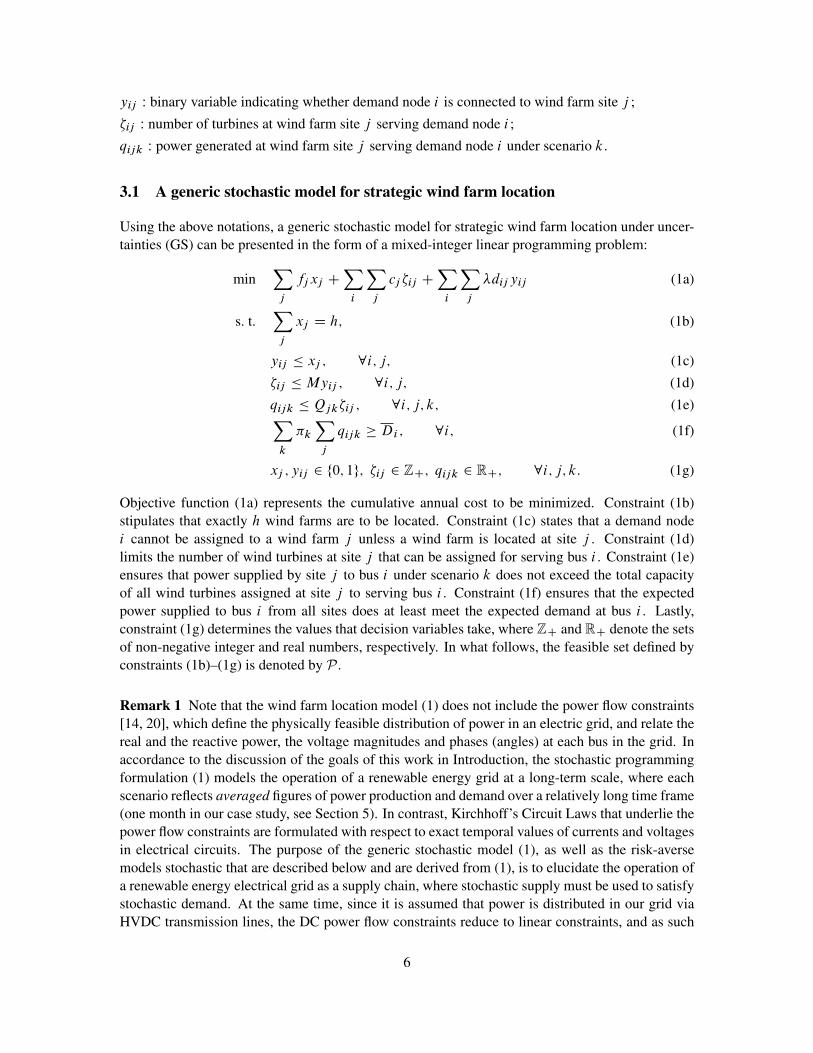
Objective function (1a) represents the cumulative annual cost to be minimized. Constraint (1b)stipulates that exactly h wind farms are to be located. Constraint (1c) states that a demand nodei cannot be assigned to a wind farm j unless a wind farm is located at site j . Constraint (1d)limits the number of wind turbines at site j that can be assigned for serving bus i . Constraint (1e)ensures that power supplied by site j to bus i under scenario k does not exceed the total capacityof all wind turbines assigned at site j to serving bus i . Constraint (1f) ensures that the expectedpower supplied to bus i from all sites does at least meet the expected demand at bus i . Lastly,constraint (1g) determines the values that decision variables take, where ZC and RC denote the setsof non-negative integer and real numbers, respectively. In what follows, the feasible set defined byconstraints (1b)–(1g) is denoted by P .

Remark 1 Note that the wind farm location model (1) does not include the power flow constraints[14, 20], which define the physically feasible distribution of power in an electric grid, and relate thereal and the reactive power, the voltage magnitudes and phases (angles) at each bus in the grid. Inaccordance to the discussion of the goals of this work in Introduction, the stochastic programmingformulation (1) models the operation of a renewable energy grid at a long-term scale, where eachscenario reflects averaged figures of power production and demand over a relatively long time frame(one month in our case study, see Section 5). In contrast, Kirchhoff’s Circuit Laws that underlie thepower flow constraints are formulated with respect to exact temporal values of currents and voltagesin electrical circuits. The purpose of the generic stochastic model (1), as well as the risk-aversemodels stochastic that are described below and are derived from (1), is to elucidate the operation ofa renewable energy electrical grid as a supply chain, where stochastic supply must be used to satisfystochastic demand. At the same time, since it is assumed that power is distributed in our grid viaHVDC transmission lines, the DC power flow constraints reduce to linear constraints, and as such

6

can be easily incorporated into the formulated models for a study of power distribution in the gridat shorter time scales. The corresponding solutions algorithms, presented in Section 4, will still beapplicable.

3.2 Risk-Averse Models for Strategic Wind Farm Location

It is easy to see that the generic stochastic optimization model (1) is prone to substantial powershortages, which may occur in particular scenarios when the power load at bus i and/or the amountof power supplied to this bus deviate from the corresponding average figures. This is a consequenceof the well-known properties of stochastic optimization models where constraints are satisfied “onaverage” [28]. In order to avoid power shortages, one may require that power load at each bus i besatisfied for every scenario !k 2 �, which can be written as

maxk

�Dik �

Xj

qijk

�� 0; 8i: (2)

This method, also known as “robust optimization” approach [27], has been acknowledged in theliterature as such that can often lead to overly conservative and exceedingly costly solutions [28]. Inaddition, enforcing the last constraint does not guarantee shortage-free power distribution in prac-tice, since the scenario data represents only a finite sample from the generally unknown distributionsof power demand and wind power production.

In this work, we pursue a risk-averse stochastic optimization approach which is supposed to avoidthe potentially large power shortages associated with the expected-value constraint (1f) as well asthe high costs associated with the “robust” constraints (2) by explicitly accounting for the risks ofpower shortages.

To quantify the risk of power shortages that may have large magnitudes but very low probabilities ofoccurring, we employ a class of statistical functional known as coherent measures of risk [3], and,more specifically, the well-known Conditional Value-at-Risk (CVaR) measure [44] and its nonlineargeneralizations, Higher Moment Coherent Risk (HMCR) measures [29].

Technically, a risk measure is a function � W X 7! R, where X is an appropriately defined linearspace of F-measurable functions X W � 7! R. Further definition of risk measures �.X/ typicallyrequires specifying whether the larger or smaller realizations of random elementX are considered tobe “risky”. Here we adopt the setup common in engineering literature, where the random variableX D X.x; !/ is assumed to represent the cost or loss associated with the decision x, and thussmaller realizations of X are preferred (the alternative assumption, that X represents payoff orreward is prevalent in economics and finance domains).

Then, �.X/ as defined above is said to be a coherent measure of risk [3, 28] if it satisfies theadditional properties of monotonicity, �.X1/ � �.X2/ for all X1 � X2; sub-additivity, �.X1 CX2/ � �.X1/C�.X2/; positive homogeneity, �.�X/ D ��.X/ for a constant � > 0; and translationinvariance, �.X C c/ D �.X/C c for any c 2 R. The monotonicity property asserts that smallerlosses bear less risk. The sub-additivity property in combination with positive homogeneity providesfor convexity of coherent risk measures, which entails that coherent measures of risk allow for riskreduction via diversification, and, importantly, admit efficient optimization of risk via the methodsof convex programming. The translation invariance property allows for efficient risk hedging, see[3] for a detailed discussion.

7

From this definition, it is easy to see that the risk measure defined as �.X/ D EX is coherent.Hence, if one defines the stochastic cost/loss function X as the energy shortage at site i , Xi .!k/ DDik�

Pj qijk , then constraints (1f) stipulating that power demand at each bus i must be satisfied on

average, can equivalently be interpreted as the requirement of non-negative risk of power shortagesat each bus i ,

�.Xi / � 0; 8i: (3)

Similarly, another trivial instance of coherent measures of risk is represented by the “maximumloss” measure, �.X/ D maxX , which associates the risk of a stochastic loss or cost X with itslargest possible realization (it is assumed here that the distribution of X has a bounded support, inthe general case the maximization operator in the definition of this risk measure must be replacedwith the essential supremum, �.X/ D ess supX , see, e.g., [28] for details). Then, the conservative-but-costly approach of ensuring that power demands are satisfied at every scenario, embodied byconstraints (2), reduces to the risk constraints of the same form (3) where � is selected as themaximum loss measure.

In order to find, as we have proposed above, an effective – both methodologically and computa-tionally – compromise between the “loose”, risk-neutral expectation-based constraints (1f) and themost conservative risk-averse constraints (2), we will employ the well-known Conditional Value-at-Risk (CVaR) measure [44]. For a given confidence level ˛ 2 .0; 1/, Conditional Value-at-RiskCVaR˛.X/ can be interpreted as the expected cost or loss that can occur with probability 1�˛ overthe prescribed time horizon, or as the average of the .1�˛/ �100% of the largest (worst) realizationsof the stochastic loss factor X . This interpretation is reflected in the fact that for a continuouslydistributed X , CVaR˛.X/ can be represented in the form of conditional expectation

CVaR˛.X/ D EŒX j X � F�1X .˛/�; (4)

where FX .t/ denotes the cumulative distribution function of X , and F�1X .˛/ is the ˛-quantile of X ,or such a deterministic value that can be exceeded by X with probability 1�˛. In financial and riskmanagement literature the ˛-quantile is also known as the Value-at-Risk at the confidence level ˛,VaR˛.X/.

In the case of general distributions of X , definition (4) does not apply, in the sense that the corre-sponding conditional expectation is not guaranteed to have coherence properties [44]. It has beenshown in [44] that in the general case CVaR˛.X/ can be represented as a convex combination ofF�1˛ .X/ and the conditional expectation of losses strictly exceeding F�1˛ .X/, with weight coef-ficients dependent on both X and ˛. A more computationally attractive definition of CVaR forgeneral loss distributions presents it as the optimal value of the following unconstrained convexoptimization problem [43, 44]:

CVaR˛.X/ D min�

�C .1 � ˛/�1E.X � �/C; (5)

where X˙ D maxf0;˙Xg. Besides being a coherent measure of risk, CVaR˛.X/ possesses anumber of other properties, such as, for example, continuity with respect to the confidence level ˛.In the context of the preceding discussion, another notable property of the CVaR measure is that, asa function of the parameter ˛, it includes both �.X/ D EX and �.X/ D ess supX as special cases:

lim˛!0

CVaR˛.X/ D EX; lim˛!1

CVaR˛.X/ D ess supX: (6)

8

Hence, to achieve a balance between the “risk-neutral” approach of ensuring that power shortages donot occur on average, and the “absolute risk-averse” approach requiring that power shortages neveroccur, one may quantify the risk of power shortages using CVaR measure with an appropriatelyselected value of confidence level ˛ 2 .0; 1/, whereby the shortage risk would be represented bythe average of .1 � ˛/ � 100% largest shortages.

To incorporate the quantification of risks of power shortages in the wind farm location model (1) viathe Conditional-Value-at-Risk measure, we define the cost/loss function X as the cumulative powershortage over all buses,

X.!k/ DXi

�Dik �

Xj

qijk

�C

; 8k: (7)

In order to have an additional degree of flexibility in our model, we include CVaR˛.X/ in theobjective of problem (1) with an appropriate weight coefficient > 0, which represents the cost (inmillions of dollars) of 1MW of power short:

minXj

fjxj CXi

Xj

cj �ij CXi

Xj

�dijyij C CVaR˛.X/

s. t. xj ; yij ; �ij ; qijk 2 P;

where X is defined by (7). Note that the cost of shortages in the objective function is non-negativedue to the fact that X.!k/ � 0 in (7). By further defining auxiliary variables Uk and �, the risk-averse CVaR-based stochastic model (CVaRS) can be formulated as follows:

minXj

fjxj CXi

Xj

cj �ij CXi

Xj

�dijyij C

��C

1

1 � ˛

Xk

�kUk

�(8a)

s. t. Uk �Xi

�Dik �

Xj

qijk

�C

� �; 8k; (8b)

Uk 2 RC; 8k; (8c)

xj ; yij ; �ij ; qijk 2 P : (8d)

By means of the Conditional Value-at-Risk measure, the risk-averse formulation (8) accounts forthe risk of power shortages as the first moment of the .1 � ˛/-tail of the shortages distribution.At the same time, the “risk” as a proxy for “large losses that have a low probability of occurring”is commonly associated in the risk management literature with “heavy tails” of distributions, andthe distributions of power shortages are well known to be heavy tailed (see, e.g., [16, 25, 35]).Therefore, it is of interest to take into account higher moments of shortage distribution in assessingthe risk of power shortages. This can be accomplished with the help of the family of Higher-MomentCoherent Risk (HMCR) measures [29]. Assuming that the space X admits a sufficient degree ofintegrability, i.e., X D Lp.�;F ;P/ for a given p � 1, the HMCR measures are defined as

HMCRp;˛.X/ D min�2R

�C .1 � ˛/�1k.X � �/Ckp; p � 1; ˛ 2 .0; 1/; (9)

where kXkp D .EjX jp/1=p. Obviously, the HMCR family contains CVaR as a special case ofp D 1.

9

Similarly to CVaR-based formulation (8), minimization of the total cost that includes the shortagerisk cost as expressed by a higher tail moment of shortage distribution is given by the followingHMCR-based stochastic optimization (HMCRS) model:

minXj

fjxj CXi

Xj

cj �ij CXi

Xj

�dijyij C ��C .1 � ˛/�1U0

�(10a)

s. t. q�1=p

kUk �

Xi

�Dik �

Xj

qijk

�C

� �; 8k; (10b)

U0 ��Up1 C : : :C U

pK

�1=p; (10c)

t � 0I Uk � 0; 8k; (10d)

xj ; yij ; �ij ; qijk 2 P : (10e)

The nonlinear inequality (10c) represents a p-order cone constraint, whence formulation (10) rep-resents a mixed-integer p-order cone programming (MIpOCP) problem. The next section discussesthe solution methods for the proposed risk-averse stochastic wind farm location models CVaRS (8)and HMCRS (10), as well as their special case, the risk-neutral GS model (1).

4 Benders Decomposition Based Branch-and-Bound Algorithms

4.1 General Formulations

The discussed formulations of GS andf CVaRS models can generally be written as mixed-integerlinear programming programming problems of the form

Z D min a>zC b>u (MILP)

s. t. AzC Bu � c;

z 2 Z � ZmC; u 2 R`C;

where z and u represent an m-dimensional vector of integer variables and an `-dimensional vectorof continuous variables, and Z is a bounded subset of Zm

C. Assume that problem MILP is bounded

and feasible. Then, it can equivalently be represented as

Z D min a>zC t .z/ (11a)

s. t. z 2 Z; (11b)

where for any given z 2 Z , function t .z/ is defined to be the optimal objective value of the linearprogramming problem

t .z/ D min b>u (12a)

s. t. Bu � c � Az; (12b)

u � 0: (12c)

Note that since set Z � ZmC

is bounded, the unboundedness of the original problem MILP is as-sociated with that of problem (12). By introducing dual variables �, we can calculate t .z/ through

10

solving its dual problem, under the assumption of boundedness of problem (12). The dual of prob-lem (12) is

t .z/ D max .c � Az/>� (SMILP)

s. t. B>� � b;� � 0:

If the feasible region of problem SMILP is empty, then the primal subproblem (12) is either un-bounded or infeasible, which implies the unboundedness or infeasibility of the original problemMILP. Otherwise, we can enumerate all extreme points .�1p ; : : : ; �

Ip /, and extreme rays .�1r ; : : : ; �

Jr /

of the feasible region of SMILP, where I and J denote the numbers of extreme points and extremerays. Therefore, the dual subproblem SMILP can be rewritten as

t .z/ D min t (13a)

s. t. .c � Az/>�jr � 0; 8j D 1; : : : ; J; (13b)

.c � Az/>�ip � t; 8i D 1; : : : ; I; (13c)

t 2 R: (13d)

By replacing t .z/ in problem (11) with that given by formulation (13), we obtain a reformulation ofthe original problem MILP:

min a>zC t (RMILP)

s. t. .c � Az/>�jr � 0; 8j D 1; : : : ; J;

.c � Az/>�ip � t; 8i D 1; : : : ; I;

z 2 Z; t 2 R:

We denote problem RMILP but only with a subset of constraints (13b) and (13c) as problem MMILP,representing the master problem of mixed-integer linear programming problem MILP.

The standard Benders decomposition scheme is then invoked, which consists in solving the “re-laxed” problem MMILP (as usual, the procedure is initialized by solving MMILP without any con-straints (13b) and (13c) and the variable t in its objective disregarded). If it is unbounded, let ��rbe the column vector in which all the corresponding simplex multipliers are negative, after simplexterminates. Therefore, ��r is an extreme ray of the feasible region of SMILP, whence a feasibilitycut

.c � Az/>��r � 0 (14a)

is added to MMILP and the problem is thus resolved until an optimal solution .z�; t�/ of MMILPis obtained. Subsequently, the dual subproblem SMILP is solved for the given z�, and let ��p bethe corresponding optimal solution, or an extreme point of its feasible region. If t .z�/ D .c �Az�/>��p > t

�, then problem MMILP is augmented with the optimality cut

.c � Az/>��p � t (14b)

and resolved.

11

The decomposition procedure stops when the condition t .z�/ D t� is satisfied. During each itera-tion, a feasibility or optimality cut is added, and an optimal solution of RMILP is obtained in a finitenumber of iterations due to finiteness of I and J [9]. The following two propositions follow readilyfrom the above discussion.

Proposition 1 If Qz 2 Z and there is an optimal solution to the dual subproblem SMILP with objec-tive value Qt D maxf.c�AQz/>� W B>� � b; � � 0g, then a> QzC Qt is an upper bound on the optimalsolution value of problem RMILP.

Proposition 2 Assume that .z�; t�/ is an optimal solution of the master problem MMILP. If theoptimal objective value of the corresponding problem SMILP is equal to t�, i.e., t� D maxf.c �Az�/>� W B>� � b; � � 0g, then .z�; t�/ is an optimal solution to the equivalent reformulation ofthe original problem RMILP.

4.2 Benders Decomposition Based Algorithm for GS and CVaRS Models

In the following, we denote problems MMILP and RMILP with relaxed integrality constraints(namely, z 2 Z � Zm

Creplaced by z 2 conv.Z/ � Rm

C) as problem MLP and problem

RLP, respectively. Furthermore, we define a node n in the branch-and-bound tree by a triple.zn; Nzn; Zn/ 2 Z2m

C� .R [ fC1g/, where .zn; Nzn/ are the bounds on z at node n and Zn is a

lower bound on ZMLP.zn;Nzn/. The problem MLP.zn; Nzn/ is defined as the problem MLP with addedconstraints zn � z � Nzn, and ZMLP.zn;Nzn/ is the corresponding optimal objective value. Similarly,for any Ozn 2 Zm

Cwe denote by SMILP.Ozn/ by replacing the variable z with the value Ozn in problem

SMILP, and by ZSMILP.Ozn/ the corresponding optimal objective value. In addition, we introduce Zand N to denote the global upper bound on ZRMILP and the set of active branch-and-bound nodes,respectively. The algorithm is described as follows (see Algorithm 1 for details).

Step 1 Initialize the set of active branch-and-bound nodes N with root node defined as .z0; Nz0; Z0/,and global upper bound Z with positive infinity.

Step 2 Select and remove a node from the set N .

Step 3 Solve problem MLP.zn; Nzn/.

Step 4 If the solution of problem MLP.zn; Nzn/ is feasible and its optimal objective value is less thanthe current global upper bound Z, go to Step 5; otherwise, fathom this node and go to Step2.

Step 5 Denote the optimal solution to problem MLP.zn; Nzn/ by .Ozn; Otn/. If the values of Ozn are allintegers, go to Step 6; otherwise, branch on this node and go to Step 2.

Step 6 Solve the problem SMILP.Ozn/. If its optimal objective value equal to Otn obtained in Step5, then update the global upper bound Z and incumbent solution, and fathom this node;otherwise, go to Step 7.

Step 7 Check the solution status of problem SMILP.Ozn/, if it is unbounded, then add a feasibilitycut to problem MLP.zn; Nzn/, go to Step 3; otherwise, check whether ZSMILP.Ozn/ > Ot

n, if it istrue, then add an optimality cut to problem MLP.zn; Nzn/, go to Step 3.

12

Algorithm 1 A Benders decomposition based branch-and-bound algorithm for GS and CVaRS mod-els

1: Set global upper bound Z WD C1; set Z0 WD �12: Set ´0r WD �1, N0r WD C1 for all r 2 f1; : : : ; mg; initialize node list N WD f.z0; Nz0; Z0/g3: while N ¤ ; do4: Select and remove a node .zn; Nzn; Zn/ from N5: Solve MLP.zn; Nzn/6: if MLP.zn; Nzn/ is feasible and ZMLP.zn;Nzn/ < Z then7: Let .Ozn; Otn/ be the optimal solution to MLP.zn; Nzn/8: if Ozn 2 Zm

Cthen

9: Solve SMILP.Ozn/10: if ZSMILP.Ozn/ D Ot

n then11: Z WD ZMLP.zn;Nzn/; update incumbent solution12: else13: if SMILP.Ozn/ is unbounded then14: Add feasibility cut (14a) to MLP.zn; Nzn/; go to 515: if ZSMILP.Ozn/ > Ot

n then16: Add optimality cut (14b) to MLP.zn; Nzn/; go to 517: else18: Select r0 in fr 2 f1; : : : ; mg W Onr … ZCg

19: Let ´r WD ´nr , N r WD Nnr for all r 2 f1; : : : ; mgnfr0g

20: Let N r0 WD b Onr0c, ´r0 WD b O

nr0c C 1

21: N WD N [˚�

zn; Nz; ZMLP.zn;Nzn/�;�z; Nzn; ZMLP.zn;Nzn/

�22: Remove every node .zn; Nzn; Zn/ 2 N such that Zn � Z23: end while

13

Proposition 3 The Benders decomposition based branch-and-bound algorithm for GS and CVaRSmodels terminates with the upper bound Z equal to the optimal objective value of original problemMILP.

Proof: The proof is omitted and is analogous to that of the more general Proposition 4 presentedin Section 4.3.1. �

Appendices A.1 and A.2, respectively, present the explicit expressions for the feasibility and opti-mality cuts that arise in the process of solving the GS and CVaRS models using the described abovealgorithm.

4.3 HMCRS Model as a Mixed-Integer p-Order Cone Programming Problem

Due to the presence of the p-order cone constraint in formulation (10),

U0 � .Up1 C : : :C U

pK /1=p; (15)

the HMCRS model represents a mixed-integer p-order cone programming problem (MIpOCP).Below we propose an algorithm for the MIpOCP HMCRS problem that combines the Bendersdecomposition with a general branch-and-bound algorithm for solving MIpOCP problems that waspresented in Vinel and Krokhmal [60]. The idea of the latter method involves solving a polyhedralapproximation of the integer relaxation of MIpOCP problem at each node of the BnB tree, and isbased on the work of Vielma et al. [59] for mixed integer second order cone programming problems(MISOCP).

Let pOCP denote the integer relaxation of the original MIpOCP problem. Then, a polyhedral ap-proximation of the pOCP relaxation is obtained by replacing nonlinear p-order cone constraintswith their polyhedral approximations. It is crucial, however, that such a polyhedral approximationbe “compact” with respect to the number of facets, since a straightforward approximation of a p-cone in RKC1 by tangent hyperplanes requires O.2K/ facets. To this end, a lifted representation ofa multidimensional p-cone is used [8, 60], which expresses a p-cone in RKC1

Cas an intersection of

K � 1 three-dimensional p-cones:

U2K�1 D U0; UKCk � .Up

2k�1C U

p

2k/1=p; k D 1; : : : ; K � 1: (16)

Then, it is easy to see that if each of the three-dimensional p-cones is replaced by its polyhedralapproximation with O.L/ facets, the resulting polyhedral approximation of multidimensional p-cone (15) will contain no more than O.KL/ facets. In particular, the following gradient-basedapproximation of three-dimensional p-cones (16) in the positive orthant R3 was employed in [60]:

UKCk � a.p/

lU2k�1 C b

.p/

lU2k; l D 0; : : : ; L; (17a)

where

a.p/

lD�cosp �l C sinp �l

� 1�pp cosp�1 �l ; b

.p/

lD�cosp �l C sinp �l

� 1�pp sinp�1 �l ; (17b)

and values �l , l D 0; : : : ; L, satisfy the condition 0 D �0 < �1 < : : : < �L D �2

.

The constructed in such a way polyhedral approximation of the pOCP relaxation of the MIpOCPproblem is solved instead of the exact nonlinear pOCP formulation at every node of the BnB tree

14

until an integer-valued solution is found. Since the employed polyhedral approximation is of outertype, its integer solution is not guaranteed to be feasible with respect to the original MIpOCP for-mulation, whence the exact pOCP relaxation needs to be solved in order to verify feasibility anddeclare incumbent or branch further (see [60] and [59] for details).

The computational advantages of this approach come from the warm-start capabilities of LP solversthat drastically reduce computational cost of solving a polyhedral approximation of relaxed problemduring BnB search in comparison to solving an exact nonlinear relaxation using an interior-pointmethod. The computational overhead associated with the necessity of invoking an exact nonlinearrelaxation for testing feasibility of the obtained solution is relatively low. It must be emphasized,however, that the effectiveness of this method is based on the premise that the employed polyhedralapproximation is relatively low-dimensional. For example, Vielma et al. [59] used a lifted polyhe-dral approximation of three-dimensional second-order cones due to Ben-Tal and Nemirovski [8],whose accuracy is exponentially small in the number of facets. The accuracy of gradient approx-imation (17) of p-cones for p ¤ 2 is only polynomially small in the number of facets, and a fastcutting plane algorithm was introduced in [30, 60] for solving the resulting polyhedral approxima-tion problems. On the other hand, it has been observed in [59, 60] that the accuracy of polyhedralapproximations used during the BnB process may be rather “crude” without a significant deterio-ration of effectiveness of the algorithm. We use this observation in the present work by employingpolyhedral approximation (16)–(17) with a small number L of facets.

Finally, to solve an exact nonlinear relaxation of MIpOCP problem during the BnB algorithm, weuse the fact that when p > 1 is a rational number, p D r=s, a p-order cone in RKC1 can beequivalently represented as a intersection of O.K log r/ three-dimensional second-order cones [7,39, 40]. Namely, the p-cone (15) is equivalent to

URk � uskU

r�s0 UR�rk ; uk � 0; k D 1; : : : ; K; (18a)

U0 �

KXkD1

uk; (18b)

where R D 2dlog2 re. Then, each nonlinear inequality (18) can be represented by dlog2 re three-dimensional “rotated” second-order cones, see [39] for details. For example, in the case of p D 3,the p-cone (15) in RKC1

Cadmits a representation via 2K quadratic cones:

U0 �

KXkD1

ukI U 2k � U0vk; v2k � ukUk; k D 1; : : : ; K:

4.3.1 Benders Decomposition Based Branch-and-Bound Algorithm for HMCRS Model

In this section, we propose an efficient method for solving the HMCRS model as a MIpOCP prob-lem that incorporates the Benders decomposition mechanism into the branch-and-bound frameworkproposed in [59, 60], and as such exploits both the mixed-integer structure of the location problemand p-order cone constraints due to the presence of risk constraints.

By employing the nomenclature introduced in Section 4.1, we represent the HMCRS model (10) inthe general form of mixed-integer nonlinear programming problem (MINLP)

Z D min a0>zC b0>u (MINLP)

15

s. t. A0zC B0u � c0;u 2 Kp;z 2 Z � ZmC; u � 0;

where Kp is a p-order cone in an appropriate high-dimensional space, such that mixed-integerlinear problem MILP is obtained from MINLP by replacing the nonlinear conic constraint with itspolyhedral approximation. The integer relaxation of MINLP, obtained by replacing constraint z 2Z � Zm

Cby z 2 conv .Z/ � Rm

C, is denoted as NLP. Then, the rest of the definitions stay

intact, namely problem RMILP denotes the equivalent Benders reformulation of problem MILP, andMMILP represents the corresponding master problem, or relaxation of RMILP, problem SMILP is thecorresponding dual subproblem of MILP, and MLP and RLP stand for problems obtained by relaxingthe integrality constraint in problem MMILP and problem RMILP, respectively. Similarly, zn, Nzn,MLP.zn; Nzn/, ZMLP.zn;Nzn/, SMILP.Ozn/, ZSMILP.Ozn/ and N are the same as described in Section 4.2.In addition, we denote the problem obtained by adding constraints zn � z � Nzn to problem NLP forany .zn; Nzn/ 2 Z2m

Cby NLP.zn; Nzn/, and the corresponding optimal objective value by ZNLP.zn;Nzn/.

Furthermore, Zn is a lower bound on ZNLP.zn;Nzn/, and Z is the global upper bound on ZMINLP. Thealgorithm is described as follows (see Algorithm 2 for details).

Step 1-5 The same as described in Section 4.2.

Step 6 Solve the problem SMILP.Ozn/. If it is unbounded, then add a feasibility cut to problemMLP.zn; Nzn/ and go to Step 3; if its optimal objective value satisfies ZSMILP.Ozn/ > Ot

n, thenadd an optimality cut to problem MLP.zn; Nzn/ and go to Step 3. If its optimal objective valueequal to Otn obtained in Step 5, go to Step 7.

Step 7 Solve problem NLP.Ozn/. If it is feasible and its optimal objective value is less than thecurrent global upper bound Z, then update the global upper bound Z and the incumbentsolution.

Step 8 If the lower and upper bounds at the current node do not coincide, zn ¤ Nzn, andZMLP.zn;Nzn/ < Z, then solve NLP.zn; Nzn/ and go to Step 9; otherwise, fathom this nodeand go to Step 2.

Step 9 If the solution of problem NLP.zn; Nzn/ is feasible and its objective value is less than thecurrent global upper bound Z, go to Step 10; otherwise, fathom this node and go to Step 2.

Step 10 Denote the optimal solution to problem NLP.zn; Nzn/ by .Qzn; Qun/. If the values of Qzn are allintegers, then update the global upper boundZ and incumbent solution, fathom this node andgo to Step 2; otherwise, branch on this node and go to Step 2.

Proposition 4 The Benders decomposition based branch-and-bound algorithm for HMCRS modelterminates with the upper boundZ equal to the optimal objective value of original problem MINLP.

Proof: First, since problem MILP is an outer linear approximation of the nonlinear problem MINLP,we may regard MILP as a relaxation of MINLP. Besides, problem MMILP could be deemed as arelaxation of problem MILP because it is a relaxation of problem RMILP, which is an equivalent

16

Algorithm 2 A Benders decomposition based branch-and-bound algorithm for HMCRS model

1: Set global upper bound Z WD C1; set Z0 WD �12: Set ´0r WD �1, N0r WD C1 for all r 2 f1; : : : ; mg; initialize node list N WD

˚�z0; Nz0; Z0

�3: while N ¤ ; do4: Select and remove a node

�zn; Nzn; Zn

�2 N

5: Solve MLP.zn; Nzn/6: if MLP.zn; Nzn/ is feasible and ZMLP.zn;Nzn/ < Z then7: Let .Ozn; Otn/ be an optimal solution to MLP.zn; Nzn/8: if Ozn 2 Zm

Cthen

9: Solve SMILP.Ozn/10: if ZSMILP.Ozn/ D Ot

n then11: Solve NLP.Ozn/.12: if NLP.Ozn/ is feasible and ZNLP.Ozn/ < Z then13: Z WD ZNLP.Ozn/

14: if zn ¤ Nzn and ZMLP.zn;Nzn/ < Z then15: Solve NLP.zn; Nzn/16: if NLP.zn; Nzn/ is feasible and ZNLP.zn;Nzn/ < Z then17: Let .Qzn; Qun/ be the optimal solution to NLP.zn; Nzn/18: if Qzn 2 Zm

Cthen

19: Z WD ZNLP.zn;Nzn/

20: else21: Select r0 in fr 2 f1; : : : ; mg W Qnr … Zg

22: Let ´r WD ´nr , N r WD Nnr for all r 2 f1; : : : ; mgnfr0g

23: Let Nzr0 WD b Qnr0c, ´r0 WD b Qnr0c C 1

24: N WD N [˚�

zn; Nz; ZNLP.zn;Nzn/�;�z; Nzn; ZNLP.zn;Nzn/

�25: else26: if SMILP.Ozn/ is unbounded then27: Add a feasibility cut (14a) to MLP.zn; Nzn/; go to 528: if ZSMILP.Ozn/ > Ot

n then29: Add an optimality cut (14b) to MLP.zn; Nzn/; go to 530: else31: Select r0 in fr 2 f1; : : : ; mg W Onr … Zg

32: Let ´r WD ´nr , N r D Nnr for all r 2 f1; : : : ; mgnfr0g

33: Let N r0 WD b Onr0c, ´r0 WD b O

nr0c C 1

34: N WD N [˚�

zn; Nz; ZMLP.zn;Nzn/�;�z; Nzn; ZMLP.zn;Nzn/

�35: Remove every node .zn; Nzn; Zn/ 2 N such that Zn � Z36: end while

17

reformulation of problem MILP. Thus, problem MMILP is a relaxation of problem MINLP, andaccordingly problem MLP is a relaxation of problem NLP.

Assuming that the polyhedral relaxation MILP is bounded, this directly implies the finiteness of thisalgorithm. We may encounter the issue that solution .Ozn; Otn/ is generated again in several nodes ifwe branch as lines 21–26 in Algorithm 2, however, this can only occur a finite number of times,see Vielma et al. [59].

In the following, we will show that an integer feasible solution to problem MINLP that has anobjective value strictly less than the cost of the current incumbent integer solution cannot exist inthe sub-tree rooted at a fathomed node. Note that a node is only fathomed in lines 6, 15, 17 and19 in Algorithm 2. In line 6, we fathom the node if MLP.zn; Nzn/ is infeasible or if the conditionZMLP.zn;Nzn/ � Z is satisfied. As it was indicated above, MLP.zn; Nzn/ is a relaxation of NLP.zn; Nzn/,and hence if MLP.zn; Nzn/ is infeasible, NLP.zn; Nzn/ will also be infeasible. In addition, one musthave ZNLP.zn;Nzn/ � ZMLP.zn;Nzn/. Therefore, an integer feasible solution which is strictly better thanthe incumbent solution cannot exist in the sub-tree rooted at such a node .zn; Nzn; Zn/. Note that inline 10, ifZSMILP.Ozn/ D Ot

n, then according to Proposition 2, Oz is in fact an integer feasible solution ofproblem RMILP, and therefore one has to check problem NLP to make further decision. In line 15,the node is fathomed when zn D Nzn or ZMLP.zn;Nzn/ � Z. If zn D Nzn, then NLP.zn; Nzn/ D NLP.Ozn/and hence the node n has been processed by lines 12–14. If ZMLP.zn;Nzn/ � Z, then ZNLP.zn;Nzn/ � Z

since MLP.zn; Nzn/ is a relaxation of NLP.zn; Nzn/. In line 17, the node is fathomed for the samereasons as described above with respect to line 6. The node is fathomed in line 19 because the bestinteger feasible solution has been found at the sub-tree rooted at the fathomed node. �

Appendix A.3 furnishes the explicit expressions for the feasibility and optimality cuts that arise inthe process of solving the HMCRS model using the described above algorithm.

5 Computational Study

5.1 Parameters and Data

This section provides description and justification for the selected data sets and the particular valuesof parameters in the three stochastic wind farm location models, GS (1), CVaRS (8), and HMCRS(10) considered in this study.

First, note that the choice of specific values for parameters h (the number of wind farms to locate),p (the order of tail moment in the HMCR measures of risk), and ˛ (the parameter controlling thetail cutoff point in both CVaR and HMCR measures of risk) are at the discretion of the decisionmaker. It can also be argued that the set of scenario probabilities �k , k D 1; : : : ; K, is in mostinstances also specified by the decision maker/analyst (e.g., in the case of historic scenario data, onemay choose whether to adopt the “physical” probabilities or apply a change of probability measureto work in the domain of “risk-neutral” probabilities, etc).

In the case study reported below, the value of the parameter h is set at h D 3, implying that threewind farms are to be established on a given set of candidate locations to serve the demand nodes.The value p in HMCR measure of risk in model (10) is chosen as p D 3, and the values of ˛ areselected at ˛ D 0:95 for the CVaRS model and ˛ D 0:90 for the HMCRS model.

18

The rest of the parameters can be separated into two categories: deterministic parameters, namely , �, fj , cj and dij , which are assumed to be constant across scenarios, and stochastic parameters,specifically Qjk and Dik , which represent the uncertainties in wind speed and consumer demand,respectively. A detailed description and rationale behind assigning specific values to these parame-ters follow next.

Deterministic Parameters The value of the parameter represents the cost of power shortages,in millions of dollars per MW short. In this study, we select values of in the range of 0 to 0.95with a step of 0.05 to conduct sensitivity analysis of obtained solutions with respect to .

We assume that �, the estimated cost of HVDC line per mile, is 1.5 million dollars. After amortizingit by 30 years, the cost is equal to 0.05 million dollars per mile per year. To evaluate the fixed costof building a wind farm, fj , we refer to Kuznia et al. [31], who estimated this value at 280 milliondollars. To account for variation of land prices at different locations, we randomly generated thevalues of parameter fj from the uniform distribution U.260; 300/, and amortized them by 20 years.Next, the cost of purchasing and installing a single wind turbine is reported to be between 1 and 2million dollars [17]. Therefore, the corresponding costs cj have been randomly generated from theuniform U.1; 2/ distribution (in millions of dollars), and amortized over 20 years. The distancesdij were randomly generated from the uniform U.200; 2000/ distribution (in miles); in addition, tomodel the “extreme” situations when building a transmission line from site j to demand node i isinfeasible or prohibitively expensive, some of the distances were randomly set equal to 1,000,000miles.

Stochastic Parameters The values of parameters Qjk and Dik are obtained either directly fromhistorical data or from Monte Carlo simulation. The corresponding scenario sets are constructed inassumption of equiprobable scenarios, i.e., �k D 1=K for all k; below we discuss the proceduresused for scenario generation.

The values of parameter Qjk representing wind turbine power output can be obtained from windspeed data. In this study, the two methods described below were used to generate scenario sets forwind speed (and, consequently, wind power production) distribution. Importantly, we assumed thatthe wind speed distributions at different site locations are statistically independent.

Historical records of monthly average wind speed data for different locations were obtained throughthe National Climatic Data Center. Typically, the monthly average wind speed data has a smallervariance and exhibits more symmetry comparing to hourly average wind speed. In this study, weassumed that the average wind speed for each site follows a normal distribution and used maximumlikelihood estimation to calculate its mean and standard deviation based on historical monthly aver-age wind speed data. Then, scenario sets for wind speed at different sites were randomly simulatedfrom the estimated normal distributions.

Another commonly used method for simulation of wind speed data relies on Weibull distribution[2, 23], whose probability density function has the form

f .x/ D

8<:�

�

�x

�

���1e�.

x�/� ; x � 0;

0; x < 0;

19

where � and � are the shape and scale parameters, respectively. To simulate wind speed distribution,the shape parameter of Weibull distribution is often chosen as � D 2, and we randomly set the scaleparameter as an integer from the range of 8 � � � 14.

The wind speed data can then be converted to power output Qjk by use of a typical power curveequation [13, 49]

P D1

2�Av3Cp;

where Cp is the power coefficient that is set equal to 0.45, A D �502 m2 represents the area sweptby the rotor blades of the wind turbine, the density of air � is equal to 1.225 kg=m3, v is the windspeed in m=s. Thus, P is the power output in watts (1 W D 1 kg �m2=s3). We then scale the resultsto MW.

The other stochastic parameter that is considered in this case study is the demand Dik at bus iunder scenario k. Similarly to the wind speed data, we also employ two approaches to generatingthe scenario set for power demand, but, in contrast to wind speed data, we assume that demands atdifferent locations may be correlated.

To construct scenario set for power using historical data, we used the data from Electric ReliabilityCouncil of Texas (ERCOT), which describes eight subsection’s electricity consumption in the stateof Texas, and scaled it by 0.02 in consideration of current wind energy penetration level (around4%) in the United States.

A second, simulated scenario set was constructed in the assumption that the power demand at eachnode i follows a mixed normal distribution XY1 C .1 � X/Y2, where X is a Bernoulli randomvariable with parameter Qp, and Y1 � N1.�; �

2/ and Y2 � N2.�; 100�2/ represent the “normal”

demand and “extreme/peak” demand, respectively. The value of parameter Qp of the Bernoulli dis-tribution was chosen as Qp D 0:9. To account for the correlation between different demand nodes,we consider a correlated multivariate distribution by additionally assuming that distributions N1 ofdifferent nodes are correlated with each other, but N2 are independent (i.e., one may not expectthat occurrence of rare events follows a certain pattern). We use the historical data from Texas toestimate the covariance matrix of demands. The samples of the “extreme” partN2.�; 100�2/ of themixed normal distribution are independently generated for each node with the �2 estimated fromthe historical data of the state of Texas.

In our numerical experiments, we constructed instances of wind farm location models of two sizes,one with 7 demand nodes and 6 candidate locations, and another with 14 demand nodes and 8 can-didate locations. The deterministic parameters for model of each size were generated as describedabove. For models of each size, the scenario sets for stochastic parameters (the wind power produc-tion and power demand) were constructed in two ways, using the historical data and simulated datain accordance to the preceding descriptions.

5.2 Computational Time Comparison

The GS, CVaRS, and HMCRS optimization models, introduced in Section 3, and the correspond-ing solution algorithms proposed in Section 4 have been implemented in C++ using CPLEX 12.5solver. In particular, the Benders decomposition-based BnB algorithms described in Sections 4.2–4.3 were implemented using CPLEX’s callback functionality, and their computational performancewas compared to CPLEX’s standard MIP and Barrier MIP solvers. Namely, in the following ta-

20

bles we denote the standard CPLEX MIP solver as “MIP”, and “MIP-B” stands for the Bendersdecomposition (Algorithm 1) algorithm applied to GS and CVaRS models. Similarly, “MISOCP”corresponds to solving the HMCRS model using the default CPLEX MIP Barrier solver as a mixedinteger second-order cone programming problem after reformulating the p-order cone constraintvia a set of second-order cones [39]. We also denote the cutting-plane based branch-and-boundalgorithm for mixed integer p-order cone programming problems due to Vinel and Krokhmal [60]as “BnB”, and the Benders decomposition based branch-and-bound algorithm (Algorithm 2) as use“BnB-B”. The computational experiments were conducted on a 3GHz PC with 4GB RAM running32-bit Windows 7.

Tables 1, 2, and 3 report the computational performance of the listed algorithms for the risk-neutral(GS), linear risk-averse (CVaRS), and nonlinear risk-averse (HMCRS) problems with varying num-ber of scenarios (K D 200, 500, 1000, and 2000), which were generated using either historicalor simulated data, for models with either 7 demand nodes and 6 candidate locations or 14 demandnodes and 8 candidate locations.

GS CVaRS HMCRS

K MIP MIP-B MIP MIP-B MISOCP BnB BnB-B

200 1.545 0.344 11.295 1.488 6.879 6.639 2.215500 6.817 1.295 245.968 4.961 31.154 33.011 5.0381000 40.185 5.242 730.632 13.026 886.495 809.142 20.467

Table 1: Computational time summary (in seconds) for various algorithms applied to GS, CVaRS,and HMCRS problems with scenario sets of K scenarios based on historical data, on a model with7 demand nodes and 6 candidate locations.

GS CVaRS HMCRS

K MIP MIP-B MIP MIP-B MISOCP BnB BnB-B

500 8.097 1.341 60.238 6.396 371.638 118.956 23.0001000 60.855 5.413 938.591 13.650 906.556 774.880 69.5642000 284.840 29.156 4061.700 27.144 10803.400 6501.980 217.885

Table 2: Computational time summary (in seconds) for various algorithms applied to GS, CVaRS,and HMCRS problems with scenario sets of K scenarios based on simulated data, on a model with7 demand nodes and 6 candidate locations.

The conducted computational study indicates that the proposed Benders decomposition allows fordrastic reductions in running time for both GS model and CVaRS models as compared to the de-fault CPLEX MIP solver, and the computational improvements tend to increase with the numberof scenarios. With regard to the nonlinear HMCRS model, we observe that the “BnB” method thatonly exploits the structure of p-order cone constraints via polyhedral approximations and the cor-responding cutting-plane algorithm, offers relatively mild improvements over “MISOCP”, the de-fault CPLEX Barrier MIP solver (which also employs polyhedral approximations). In contrast, the

21

GS CVaRS HMCRS

K MIP MIP-B MIP MIP-B MISOCP BnB BnB-B

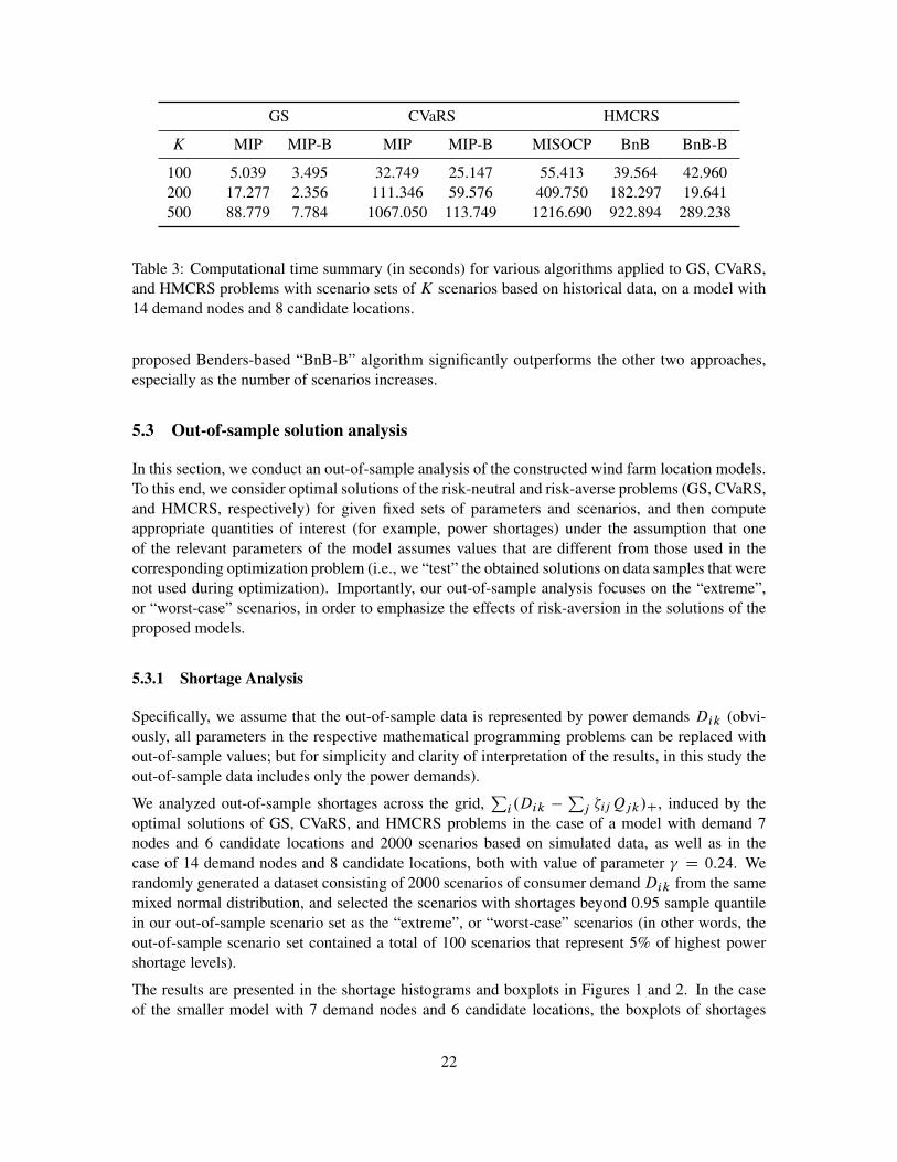
100 5.039 3.495 32.749 25.147 55.413 39.564 42.960200 17.277 2.356 111.346 59.576 409.750 182.297 19.641500 88.779 7.784 1067.050 113.749 1216.690 922.894 289.238

Table 3: Computational time summary (in seconds) for various algorithms applied to GS, CVaRS,and HMCRS problems with scenario sets of K scenarios based on historical data, on a model with14 demand nodes and 8 candidate locations.

proposed Benders-based “BnB-B” algorithm significantly outperforms the other two approaches,especially as the number of scenarios increases.

5.3 Out-of-sample solution analysis

In this section, we conduct an out-of-sample analysis of the constructed wind farm location models.To this end, we consider optimal solutions of the risk-neutral and risk-averse problems (GS, CVaRS,and HMCRS, respectively) for given fixed sets of parameters and scenarios, and then computeappropriate quantities of interest (for example, power shortages) under the assumption that oneof the relevant parameters of the model assumes values that are different from those used in thecorresponding optimization problem (i.e., we “test” the obtained solutions on data samples that werenot used during optimization). Importantly, our out-of-sample analysis focuses on the “extreme”,or “worst-case” scenarios, in order to emphasize the effects of risk-aversion in the solutions of theproposed models.

5.3.1 Shortage Analysis

Specifically, we assume that the out-of-sample data is represented by power demands Dik (obvi-ously, all parameters in the respective mathematical programming problems can be replaced without-of-sample values; but for simplicity and clarity of interpretation of the results, in this study theout-of-sample data includes only the power demands).

We analyzed out-of-sample shortages across the grid,Pi .Dik �

Pj �ijQjk/C, induced by the

optimal solutions of GS, CVaRS, and HMCRS problems in the case of a model with demand 7nodes and 6 candidate locations and 2000 scenarios based on simulated data, as well as in thecase of 14 demand nodes and 8 candidate locations, both with value of parameter D 0:24. Werandomly generated a dataset consisting of 2000 scenarios of consumer demandDik from the samemixed normal distribution, and selected the scenarios with shortages beyond 0.95 sample quantilein our out-of-sample scenario set as the “extreme”, or “worst-case” scenarios (in other words, theout-of-sample scenario set contained a total of 100 scenarios that represent 5% of highest powershortage levels).

The results are presented in the shortage histograms and boxplots in Figures 1 and 2. In the caseof the smaller model with 7 demand nodes and 6 candidate locations, the boxplots of shortages

22

indicate that both risk-averse models, HMCRS and CVaRS, significantly outperform the risk-neutralGS model. The CVaRS model has smaller 0.75 quantile value of shortages than HMCRS model,but it has larger extreme points. This observation is in accord with sensitivity analysis presentedin the next section. Analysis of shortage histograms shows that all shortages for HMCRS modelare within 500 MW, and most of its shortages fall in the range of [0, 50) MW, while the fractionof zero shortages exceeds 30%. As regards the CVaRS model, shortage has exceeded 500 MW inone scenario, but most of its shortages do not exceed 250 MW, also with a high fraction of zeroshortages. In contrast, “extreme” out-of-sample power shortages in GS model are always non-zeroand fall mainly between 500 MW and 1000 MW, and can be as high as 1500 MW.

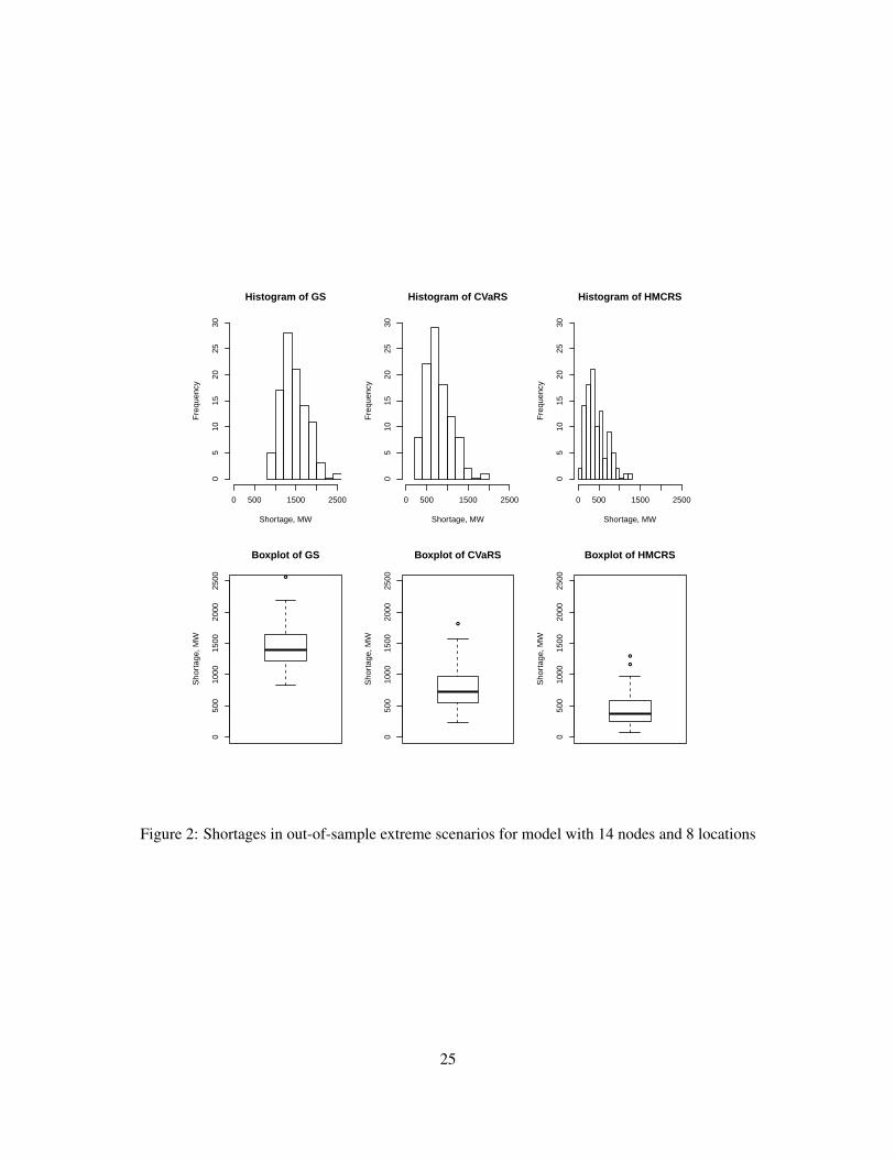
Similarly, in the case of models with 14 demand nodes and 8 candidate locations, boxplots in Fig-ure 2 indicate that the HMCRS model has the lowest 0.25 quantile, median, 0.75 quantile, etc., andCVaRS model performs much better than the GS model. The histograms of power shortages indicatethat over 20% of out-of-sample shortages are within Œ0; 250/ MW for HMCRS model. However,no shortages fall into this range in the case of CVaRS and GS models. Also, 98% of “extreme”out-of-sample shortages are below 1000 MW for HMCRS model. Although over 70% of “extreme”out-of-sample shortages are under 1000 MW for CVaRS model, there is a substantial number ofout-of-sample shortages within [1000,1500) MW, and even reaching 2000 MW in one scenario. Asregards the GS model, most of its shortages are between 1000 MW and 2000 MW, and it has nearly5% of “extreme” out-of-sample shortages beyond 2000 MW. The largest shortage that was observedin the GS model is close to 2500 MW.

5.3.2 Sensitivity with Respect to Shortage Penalty Parameter

Recall that the sensitivity to power shortages of the risk-averse CVaRS and HMCRS models isdetermined by the parameter , which represents the dollar cost of 1 MW of power short. Therisk-neutral GS model is insensitive to (does not contain) the parameter , and, moreover, for thevalue of D 0, all three models yield the same solutions. In this section, we evaluate severalaspects of the performance of the GS, CVaRS, and HMCRS models with respect to different levelsof sensitivity to power shortages, corresponding to varying the value of the parameter from 0 to0.95. Obviously, the solution of the GS model would not change with , and can be considered asthe “reference” point in this comparison.

To evaluate the performance of three models, we consider four criteria: (1) the amortized annualcost, (2) the mean cumulative shortage across the grid, (3) the number of shortage scenarios, i.e., thescenarios under which shortages occur, and (4) the mean number of demand nodes that experienceshortages. The annual cost is computed as

Pj fjxjC

Pi

Pj cj �ijC

Pi

Pj �dijyij ; according to

Section 5.3, the cumulative shortage at scenario k is defined asPi .Dik �

Pj �ijQjk/C, and thus

mean shortage is EŒPi .Dik�

Pj �ijQjk/C�. As in the previous section, the out-of-sample analysis

is conducted, in the sense that all the four criteria are evaluated on the set of 100 “extreme” out-of-sample scenarios determined as described above, e.g., the mean shortage and the mean number ofdemand nodes with shortages should be interpreted as a conditional expectations. The four criteriaare thus computed for the case of 7 demand nodes and 6 candidate locations and 2,000 scenarios,and values of varying from 0 to 0.95 with a step of 0.05. The results are presented in Figure 3,where the horizontal (constant) lines correspond to the GS model.

As expected, the annual costs of CVaRS and HMCRS models increase with . In contrast, meanshortage and mean number of shortage nodes in the CVaRS and HMCRS models decrease sharply

23

Histogram of GS

Shortage, MW

Fre

quen

cy

0 500 1000 1500

010

2030

40

Histogram of CVaRS

Shortage, MW

Fre

quen

cy

0 500 1000 1500

010

2030

40

Histogram of HMCRS

Shortage, MW

Fre

quen

cy

0 500 1000 1500

010

2030

40

●

050

010

0015

00

Boxplot of GS

Sho

rtag

e, M

W

●

●

●

●

050

010

0015

00

Boxplot of CVaRS

Sho

rtag

e, M

W

●

050

010

0015

00Boxplot of HMCRS

Sho

rtag

e, M

W

Figure 1: Shortages in out-of-sample extreme scenarios for model with 7 nodes and 6 locations

24

Histogram of GS

Shortage, MW

Fre

quen

cy

0 500 1500 2500

05

1015

2025

30

Histogram of CVaRS

Shortage, MW

Fre

quen

cy

0 500 1500 2500

05

1015

2025

30

Histogram of HMCRS

Shortage, MW

Fre

quen

cy

0 500 1500 2500

05

1015

2025

30

●

050

010

0015

0020

0025

00

Boxplot of GS

Sho

rtag

e, M

W

●

050

010

0015

0020

0025

00

Boxplot of CVaRS

Sho

rtag

e, M

W

●

●

050

010

0015

0020

0025

00Boxplot of HMCRS

Sho

rtag

e, M

W

Figure 2: Shortages in out-of-sample extreme scenarios for model with 14 nodes and 8 locations

25

0.0 0.2 0.4 0.6 0.8

300

350

400

450

500

Gamma

Cos

t

GSCVaRSHMCRS

0.0 0.2 0.4 0.6 0.8

020

040

060

0

Gamma

Mea

n S

hort

age

GSCVaRSHMCRS

0.0 0.2 0.4 0.6 0.8

020

4060

8010

0

Gamma

No.

of S

hort

age

Sce

nario

s

GSCVaRSHMCRS

0.0 0.2 0.4 0.6 0.8

01

23

45

6

Gamma

Mea

n N

o. o

f Sho

rtag

e N

odes

GSCVaRSHMCRS

Figure 3: Out-of-sample performance of GS, CVaRS and HMCRS with regard to

26

with . Compared with the CVaRS model, the HMCRS model always performs better in termsof criteria (2)–(4), except for values around 0.5, but incurs higher annual costs. In conclusion,CVaRS and HMCRS models could be tuned to fit user’s risk-averse preference so as to achievebetter risk control of power shortages.

6 Conclusions

In this paper, we have considered three different stochastic optimization models for strategic windfarm location and operation: a risk-neutral model, a two models where risk preferences are repre-sented by a linear risk measure (Conditional Value-at-Risk), and a nonlinear risk measure (Higher-Moment Coherent Risk measure). We proposed a branch-and-bound algorithm based on Bendersdecomposition technique to solve the resulting linear and p-order cone mixed-integer programmingproblems. The conducted numerical study demonstrates the efficiency of developed algorithms, andalso indicates the risk-averse models allow for drastic reduction of wind power shortages, and caneffectively be used in strategic location and planning problems.

Acknowledgments

This work was supported in part by the NSF grant DMI 0457473 and DTRA grant HDTRA1-14-1-0065.

References[1] Abbey, C. and Joos, G. (2009) “A stochastic optimization approach to rating of energy storage systems

in wind-diesel isolated grids,” Power Systems, IEEE Transactions on, 24 (1), 418–426.

[2] Aksoy, H., Toprak, Z. F., Aytek, A., and Unal, N. E. (2004) “Stochastic generation of hourly mean windspeed data,” Renewable energy, 29 (14), 2111–2131.

[3] Artzner, P., Delbaen, F., Eber, J.-M., and Heath, D. (1999) “Coherent measures of risk,” Mathematicalfinance, 9 (3), 203–228.

[4] Azaron, A., Brown, K., Tarim, S., and Modarres, M. (2008) “A multi-objective stochastic programmingapproach for supply chain design considering risk,” International Journal of Production Economics,116 (1), 129–138.

[5] Baghalian, A., Rezapour, S., and Farahani, R. Z. (2013) “Robust supply chain network design withservice level against disruptions and demand uncertainties: A real-life case,” European Journal of Op-erational Research, 227 (1), 199–215.

[6] Baron, O., Milner, J., and Naseraldin, H. (2011) “Facility location: A robust optimization approach,”Production and Operations Management, 20 (5), 772–785.

[7] Ben-Tal, A. and Nemirovski, A. (2001) Lectures on modern convex optimization: analysis, algorithms,and engineering applications, volume 2 of MPS/SIAM Series on Optimization, SIAM.

[8] Ben-Tal, A. and Nemirovski, A. (2001) “On polyhedral approximations of the second-order cone,”Mathematics of Operations Research, 26 (2), 193–205.

27

[9] Benders, J. F. (1962) “Partitioning procedures for solving mixed-variables programming problems,”Numerische mathematik, 4 (1), 238–252.

[10] Berman, O. and Drezner, Z. (2008) “The p-median problem under uncertainty,” European Journal ofOperational Research, 189 (1), 19–30.

[11] Berman, O., Krass, D., and Menezes, M. B. (2007) “Facility reliability issues in network p-medianproblems: strategic centralization and co-location effects,” Operations Research, 55 (2), 332–350.

[12] Burke, D. J. and O’Malley, M. (2008) “Optimal wind power location on transmission systems-a proba-bilistic load flow approach,” in: “Probabilistic Methods Applied to Power Systems, 2008. PMAPS’08.Proceedings of the 10th International Conference on,” 1–8, IEEE.

[13] Burton, T., Jenkins, N., Sharpe, D., and Bossanyi, E. (2011) Wind energy handbook, John Wiley &Sons.

[14] Carpentier, J. (1962) “Contribution a letude du dispatching economique,” Bulletin de la Societe Fran-caise des Electriciens, 3 (1), 431–447.

[15] Chen, G., Daskin, M. S., Shen, Z.-J. M., and Uryasev, S. (2006) “The ˛-reliable mean-excess regretmodel for stochastic facility location modeling,” Naval Research Logistics (NRL), 53 (7), 617–626.

[16] Clauset, A., Shalizi, C. R., and Newman, M. E. (2009) “Power-law distributions in empirical data,”SIAM review, 51 (4), 661–703.

[17] Conserve Energy Future (2013) “Cost of Wind Energy,” http://www.conserve-energy-future.com/WindEnergyCost.php, [Online; accessed 12-Nov-2013].

[18] Cui, T., Ouyang, Y., and Shen, Z.-J. M. (2010) “Reliable facility location design under the risk ofdisruptions,” Operations Research, 58 (4-part-1), 998–1011.

[19] Daskin, M. S., Hesse, S. M., and Revelle, C. S. (1997) “˛-reliable p-minimax regret: A new model forstrategic facility location modeling,” Location Science, 5 (4), 227–246.

[20] Dommel, H. W. and Tinney, W. F. (1968) “Optimal power flow solutions,” IEEE transactions on powerapparatus and systems, (10), 1866–1876.

[21] Drezner, Z. (1987) “Heuristic solution methods for two location problems with unreliable facilities,”Journal of the Operational Research Society, 509–514.

[22] Ekren, O. and Ekren, B. Y. (2010) “Size optimization of a PV/wind hybrid energy conversion systemwith battery storage using simulated annealing,” Applied Energy, 87 (2), 592–598.

[23] Garcia, A., Torres, J., Prieto, E., and De Francisco, A. (1998) “Fitting wind speed distributions: a casestudy,” Solar Energy, 62 (2), 139–144.

[24] Ghiani, G., Laporte, G., and Musmanno, R. (2004) Introduction to logistics systems planning and con-trol, John Wiley & Sons, New York.

[25] Glass, R., Beyeler, W., Stamber, K., Glass, L., LaViolette, R., Conrad, S., Brodsky, N., Brown, T.,Scholand, A., and Ehlen, M. (2005) “Simulation and Analysis of Cascading Failure in Critical Infras-tructure,” Technical report, Sandia National Laboratories.

[26] Katsigiannis, Y. and Georgilakis, P. (2008) “Optimal sizing of small isolated hybrid power systemsusing tabu search,” Journal of Optoelectronics and Advanced Materials, 10 (5), 1241.

[27] Kouvelis, P. and Yu, G. (1997) Robust discrete optimization and its applications, Kluwer AcademicPublishers, Dordrecht.

28

[28] Krokhmal, P., Zabarankin, M., and Uryasev, S. (2011) “Modeling and optimization of risk,” Surveys inOperations Research and Management Science, 16 (2), 49–66.

[29] Krokhmal, P. A. (2007) “Higher moment coherent risk measures,” Quantitative Finance, 7 (4), 373–387.

[30] Krokhmal, P. A. and Soberanis, P. (2010) “Risk optimization with p-order conic constraints: A linearprogramming approach,” European Journal of Operational Research, 201 (3), 653–671.

[31] Kuznia, L., Zeng, B., Centeno, G., and Miao, Z. (2011) “Stochastic optimization for power systemconfiguration with renewable energy in remote areas,” Annals of Operations Research, 1–22.

[32] Lopez, A., Roberts, B., Heimiller, D., Blair, N., and Porro, G. (2012) “U.S. renewable energy technicalpotentials: a GIS-based analysis,” Technical report, National Renewable Energy Laboratory.

[33] Louveaux, F. (1986) “Discrete stochastic location models,” Annals of Operations research, 6 (2), 21–34.

[34] Lu, M., Ran, L., and Shen, Z.-J. M. (2015) “Reliable Facility Location Design Under Uncertain Corre-lated Disruptions,” Manufacturing & Service Operations Management, 17 (4), 445–455.

[35] Mei, S., Zhang, X., and Cao, M. (2011) Power grid complexity, Springer.

[36] Melo, M. T., Nickel, S., and Saldanha-Da-Gama, F. (2009) “Facility location and supply chainmanagement–A review,” European journal of operational research, 196 (2), 401–412.

[37] Mirchandani, P. B. and Oudjit, A. (1980) “Localizing 2-medians on probabilistic and deterministic treenetworks,” Networks, 10 (4), 329–350.

[38] Mirchandani, P. B., Oudjit, A., and Wong, R. T. (1985) “‘Multidimensional’ extensions and a nesteddual approach for the m-median problem,” European Journal of Operational Research, 21 (1), 121–137.

[39] Morenko, Y., Vinel, A., Yu, Z., and Krokhmal, P. (2013) “On p-cone linear discrimination,” EuropeanJournal of Operational Research, 231, 784–789.

[40] Nesterov, Y., Nemirovskii, A., and Ye, Y. (1994) Interior-point polynomial algorithms in convex pro-gramming, volume 13 of Studies in Applied Mathematics, SIAM, Philadelphia, PA.

[41] Owen, S. H. and Daskin, M. S. (1998) “Strategic facility location: A review,” European Journal ofOperational Research, 111 (3), 423–447.

[42] Peng, P., Snyder, L. V., Lim, A., and Liu, Z. (2011) “Reliable logistics networks design with facilitydisruptions,” Transportation Research Part B: Methodological, 45 (8), 1190–1211.

[43] Rockafellar, R. T. and Uryasev, S. (2000) “Optimization of conditional value-at-risk,” Journal of risk,2, 21–42.

[44] Rockafellar, R. T. and Uryasev, S. (2002) “Conditional value-at-risk for general loss distributions,”Journal of Banking & Finance, 26 (7), 1443–1471.

[45] Roques, F., Hiroux, C., and Saguan, M. (2010) “Optimal wind power deployment in Europea portfolioapproach,” Energy Policy, 38 (7), 3245–3256.

[46] Santoso, T., Ahmed, S., Goetschalckx, M., and Shapiro, A. (2005) “A stochastic programming ap-proach for supply chain network design under uncertainty,” European Journal of Operational Research,167 (1), 96–115.

[47] Schutz, P., Tomasgard, A., and Ahmed, S. (2009) “Supply chain design under uncertainty using sampleaverage approximation and dual decomposition,” European Journal of Operational Research, 199 (2),409–419.

29

[48] Schwartz, M., Heimiller, D., Haymes, S., and Walt, M. (2010) “Assessment of offshore wind energyresources for the United States,” Technical report, National Renewable Energy Laboratory.

[49] Scott, W. R. and Powell, W. B. (2012) “Approximate dynamic programming for energy storage withnew results on instrumental variables and projected Bellman errors,” Submitted to Operations Research(Under Review).

[50] Senjyu, T., Hayashi, D., Yona, A., Urasaki, N., and Funabashi, T. (2007) “Optimal configuration ofpower generating systems in isolated island with renewable energy,” Renewable Energy, 32 (11), 1917–1933.

[51] Shapiro, J. F. (2001) Modeling the Supply Chain, Duxbury Press, Pacific Grove, CA.

[52] Shen, Z.-J. M., Zhan, R. L., and Zhang, J. (2011) “The reliable facility location problem: Formulations,heuristics, and approximation algorithms,” INFORMS Journal on Computing, 23 (3), 470–482.

[53] Sheppard, E. (1974) “A conceptual framework for dynamic location-allocation analysis,” Environmentand Planning A, 6 (5), 547–564.

[54] Simchi-Levi, D., Kaminsky, P., and Simchi-Levi, E. (2004) Managing the Supply Chain: The DefinitiveGuide for the Supply Chain Professional, McGraw-Hill, New York.

[55] Snyder, L. V. (2006) “Facility location under uncertainty: a review,” IIE Transactions, 38 (7), 547–564.

[56] Snyder, L. V., Atan, Z., Peng, P., Rong, Y., Schmitt, A. J., and Sinsoysal, B. (2015) “OR/MS models forsupply chain disruptions: A review,” IIE Transactions, 1–21.

[57] Snyder, L. V. and Daskin, M. S. (2005) “Reliability models for facility location: the expected failurecost case,” Transportation Science, 39 (3), 400–416.

[58] Snyder, L. V. and Daskin, M. S. (2006) “Stochastic p-robust location problems,” IIE Transactions,38 (11), 971–985.

[59] Vielma, J. P., Ahmed, S., and Nemhauser, G. L. (2008) “A lifted linear programming branch-and-boundalgorithm for mixed-integer conic quadratic programs,” INFORMS Journal on Computing, 20 (3), 438–450.

[60] Vinel, A. and Krokhmal, P. (2014) “Polyhedral approximations in p-order cone programming,” Opti-mization Methods & Software, 29 (6), 1210–1237.

[61] Weaver, J. R. and Church, R. L. (1983) “Computational procedures for location problems on stochasticnetworks,” Transportation Science, 17 (2), 168–180.

[62] World Wind Energy Association (2014) “2014 Half-year Report,” Technical report, World Wind EnergyAssociation.

A Feasibility and Optimality Cuts

A.1 Feasibility Cuts for GS Model

The generic stochastic model GS (1) can be written in the form of problem MILP, where the integer-valuedvector z contains variables xj , yij , and �ij , and nonnegative vector u contains variables pijk . Then, thecorresponding problem (11) has the form

Z D minXj

fjxj CXi

Xj

cj �ij CXi

Xj

�dijyij (19a)

30

s. t.Xj

xj D h; (19b)

yij � xj ; 8i; j; (19c)�ij �Myij ; 8i; j; (19d)xj ; yij 2 f0; 1g; �ij 2 ZC; 8i; j; k; (19e)

where the function t .z/ defined as the optimal objective of subproblem (12) is equal to either 0 when theproblem

t .z/ D min 0 (20a)s. t. qijk � Qjk�ij ; 8i; j; k; (20b)X

k

�kXj

qijk � Di ; 8i; (20c)

qijk � 0; (20d)

is feasible for the given values of �ij , or t .z/ D C1when (20) is infeasible. Obviously, if Oz D . Oxj ; Oyij ; O�ij / isan optimal solution of (19) such that (20) has a feasible Oqijk for the given O�ij , then .Oz; Ou/ D . Oxj ; Oyij ; O�ij ; Oqijk/is an optimal solution of the original problem (1). On the other hand, if (20) is infeasible, then the corre-sponding Oz should be eliminated from the feasible region of the master problem (19). In accordance to thedescribed above algorithm, this is accomplished by augmenting (19) with feasibility cutsX

i

Xj

Xk

Qjk O ijk�ij �Xi

DiOi � 0; (21)

where . O ijk ; Oi / is an extreme ray of the dual SMILP.Oz/ of problem (20), which takes the form

t .Oz/ D maxXi

Xj

Xk

Qjk O�ij˛ijk �Xi

Diˇi (22a)

s. t. ˛ijk � �kˇi � 0; 8i; j; k; (22b)˛ijk ; ˇi � 0; 8i; j; k: (22c)

Clearly, no optimality cuts are added to (19) since (20) is a “feasibility” subproblem.

A.2 Feasibility and Optimality Cuts for CVaRS Model

Analogously to above, the CVaRS model (8) can be reformulated in the form (11)–(12) as follows

Z D minXj

fjxj CXi

Xj

cj �ij CXi

Xj

�dijyij C t (23a)

s. t.Xj

xj D h; (23b)

yij � xj ; 8i; j; (23c)�ij �Myij ; 8i; j; (23d)xj ; yij 2 f0; 1g; �ij 2 ZC; t 2 R; (23e)

with the subproblem (20) defined as:

t .Oz/ D min �C1

1 � ˛

Xk

�kUk (24a)

31

s. t. qijk � Qjk O�ij ; 8i; j; k; (24b)Xk

�kXj

qijk � Di ; 8i; (24c)

wik � Dik �Xj

qijk ; 8i; k; (24d)

Uk �Xi

wik � �; 8k; (24e)

wik ; qijk ; Uk � 0; 8i; j; k: (24f)

Let ˛ijk , �i , ˇik , and �k be the dual variables associated with constraints (24b), (24c), (24d) and (24e)respectively. Then, the dual of subproblem becomes

t .z/ D maxXi

Xj

Xk

Qjk O�ij˛ijk �Xi

Xk

Dikˇik �Xi

Di�i (25a)

s. t. ˛ijk � ˇik � �k�i � 0; 8i; j; k; (25b)

� �k �1

1 � ˛�k ; 8k; (25c)

� ˇik C �k � 0; 8i; k; (25d)

�

Xk

�k � 1; (25e)

˛ijk ; �i ; ˇik ; �k � 0; 8i; j; k: (25f)

If, for a given set of values O�ij , where . Oxj ; Oyij ; O�ij ; Ot / is an optimal solution of (23), problem (25) isunbounded, let . O ijk ; Oik ; O�i / be an extreme ray of the feasible region of (25), such that

Pi

Pj

Pk

.Qjk O ijk/ O�ij �Pi

PkDik

Oik �

Pi Di O�i > 0. Then, the feasibility cutX

i

Xj

Xk

Qjk O ijk�ij �Xi

Xk

Dik Oik �Xi

Di O�i � 0; (26)

is added to the master problem. If, on the other hand, the optimal objective t� D t .Oz/ of (25) is finite andsuch that Ot < t�, the following optimality cut is added to the master:X

i

Xj

Xk

Qjk O ijk�ij �Xi

Xk

Dik Oik �Xi

Di O�i � t; (27)

where . O ijk ; Oik ; O�i / is an optimal solution of (25).

A.3 Feasibility and Optimality Cuts for HMCRS Model

The polyhedral approximation of the HMCRS model (10) can be written in the form of a mixed-integer linearproblem MILP where, as before, the integer-valued vector z comprises variables xj , yij , and �ij , so that thecorresponding problem (11) has the form

Z D minXj

fjxj CXi

Xj

cj �ij CXi

Xj

�dijyij C t (28a)

s. t.Xj

xj D h; (28b)

yij � xj ; 8i; j; (28c)

32

�ij �Myij ; 8i; j; (28d)xj ; yij 2 f0; 1g; �ij 2 ZC; t � 0; (28e)

and the subproblem (12), whose optimal objective t .z/ defines the value of variable t above, takes the form

t .z/ D min �C .1 � ˛/�1U2K�1 (29a)s. t. qijk � Qjk�ij ; 8i; j; n; (29b)X

k

�kXj

qijk � Di ; 8i; (29c)

wik � Dik �Xj

qijk ; 8i; k; (29d)

Uk � �1=p

k

�Xi

wik � �

�; 8k; (29e)

UKCr � a.p/

lU2r�1 C b

.p/

lU2r ; 8r; l; (29f)

wik ; qijk ; Uk � 0; (29g)

where the nonnegative variables pijk , wik , and Uk comprise the vector u, see (12).

Let ˛ijk , �i , ˇik , �k , and �lk be the multipliers associated with constraints (29b), (29c), (29d), (29e), and(29f), respectively. Then, the dual of subproblem (29) can be written as

t .z/ D maxXi

Xj

Xk

Qjk�ij˛ijk �Xi

Xk

Dikˇik �Xi

Di�i (30a)

s. t. ˛ijk � ˇik � �k�i � 0; 8i; j; k; (30b)� ˇik C �k � 0; 8i; k; (30c)

�

Xk

�k � 1; (30d)

� �k CXl

a.p/

l�ld k2 e

� 0; 8k D 1; 3; : : : ; K � 1; (30e)

� �k CXl

b.p/

l�ld k2 e

� 0; 8k D 2; 4; : : : ; K; (30f)

Xl

A.p/

l�l.K2 Cd

k2 e/�

Xl

�lk � 0; 8k D 1; 3; : : : ; K � 3; (30g)

Xl

B.p/

l�l.K2 Cd

k2 e/�

Xl

�lk � 0; 8k D 2; 4; : : : ; K � 2; (30h)

�

Xl

�l.K�1/ �1

1 � ˛; (30i)

˛ijk ; �i ; ˇik ; �k ; �lk � 0: (30j)

For the sake of simplicity, we assume K is an even number. If, for a given optimal value Oz obtained from(28), problem (30) is unbounded, let . O ; O ; O�/ be an extreme ray of (30), such that

Pi

Pj

Pk Qjk O ijk

O�ij �Pi

PkDik

Oik �

Pi Di O�i > 0. Then, a feasibility cutX

i

Xj

Xk

Qjk O ijk�ij �Xi

Xk

Dik Oik �Xi

Di O�i � 0; (31)

is added to (28). Conversely, let Ot and t� denote an optimal value of t in the master problem (28), and theoptimal objective function value of problem (30), respectively. If Ot < t�, then an optimality cutX

i

Xj

Xk

Qjk O ijk�ij �Xi

Xk

Dik Oik �Xi

Di O�i � t; (32)

33

is added to the master problem (28).

34