risk aggregation and diversification - cia-ica.ca · and received approval for distribution from...
TRANSCRIPT
Research reports do not necessarily represent the views of the Canadian Institute of Actuaries. Members should be familiar with research reports. Research reports do not constitute
standards of practice and therefore are not binding. Research reports may or may not be in compliance with standards of practice. Responsibility for the manner of application of
standards of practice in specific circumstances remains that of the members.
Research Paper
Risk Aggregation and Diversification
Committee on Risk Management and Capital Requirements
April 2016
Document 216037
Ce document est disponible en français © 2016 Canadian Institute of Actuaries

1740-360 Albert, Ottawa, ON K1R 7X7 613-236-8196 613-233-4552 [email protected] / [email protected] cia-ica.ca
MEMORANDUM To: All Fellows, Affiliates, Associates, and Correspondents of the Canadian
Institute of Actuaries
From: Pierre Dionne, Chair Practice Council Leonard Pressey, Chair Committee on Risk Management and Capital Requirements
Date: April 14, 2016 Subject: Research Paper on Risk Aggregation and Diversification
The Canadian Institute of Actuaries (CIA) Committee on Risk Management and Capital Requirements (CRMCR) sponsored a research paper on risk aggregation and diversification. The literature on this topic is rapidly expanding and new approaches for dealing with risk aggregation and its impact on model risk are expected to be the topic of significant study in the future. The focus for the research was as follows:
• Literature search of methods used internationally to measure and recognize the effects of combining diverse risks (e.g., insurance, credit, market, operational, and other risks). Sources may include academic literature, regulatory approaches to risk-based capital requirements, actuarial literature, and insurance industry approaches.
• While the focus is on life and non-life insurance enterprises, approaches taken in other industries may have relevance to the insurance sector.
The researchers started with a review of the academic literature on risk aggregation as well as risk-based regulatory approaches. In addition, they drew on their own research and publications on risk aggregation and diversification to expand on the future of risk aggregation approaches. These reviews were then used to summarize current practices and point out the advantages and disadvantages of the different approaches for risk aggregation and their limitations, including theoretical correctness, calibration issues, and further practical implementation.
In accordance with the Institute’s Policy on Due Process for the Approval of Guidance Material other than Standards of Practice and Research Documents, this research paper has been prepared by the Committee on Risk Management and Capital Requirements, and received approval for distribution from the Practice Council on April 5, 2016.
The CRMCR acknowledges the assistance of the Joint Risk Management Section of the Society of Actuaries (SOA), the CIA, the Casualty Actuarial Society (CAS), and the CIA Head Office staff.

3
If you have any questions or comments regarding this research paper, please contact Leonard Pressey, Chair, Committee on Risk Management and Capital Requirements at [email protected].
PD, LP

Research Paper April 2016
4
Risk Aggregation and Diversification
C. Bernard S. Vanduffel
February 23, 2016
Table of Contents Overview ......................................................................................................................................... 6
Introduction .................................................................................................................................... 6
1. Measuring Aggregate Risk ...................................................................................................... 8
1.1 Coherent Risk Measures .................................................................................................. 9
1.2 Backtesting and Robustness of Risk Measures .............................................................. 10
2. Aggregation and Diversification ............................................................................................ 12
2.1 Diversification Benefits and Subadditivity ..................................................................... 12
2.2 The Fallacy of Using Correlations Only........................................................................... 13
2.3 The Impact of Microcorrelations.................................................................................... 15
2.4 Fitting a Multivariate Distribution .................................................................................. 16
2.5 Summary ........................................................................................................................ 17
3. Overview of Current Regulation ........................................................................................... 18
3.1 Regulatory Frameworks ................................................................................................. 18
3.2 Comparison and Comments on International Regulatory Frameworks ........................ 19
4. Model Risk on Dependence .................................................................................................. 20
5. Conclusions ........................................................................................................................... 23
Appendix A – Model Risk of Dependence when Aggregating Risks ............................................. 25
A.1 Convex Upper and Lower Bounds .................................................................................. 26
A.2 Rearrangement Algorithm ............................................................................................. 27
A.3 Example of Application of the RA .................................................................................. 28
A.4 Model Risk on Dependence on Variance ....................................................................... 29
A.5 Model Risk on Dependence on VaR ............................................................................... 30
Appendix B – Model Risk of Dependence when Aggregating Risks and Model Risk Quantification .............................................................................. 33
B.1 Theoretical Setting and Assumptions ............................................................................ 35
B.2 Practical Framework for the Non-Parametric Approach ............................................... 37

Research Paper April 2016
5
B.3 Bounds on a Given Risk Measure ................................................................................... 40
B.3.1 Theoretical Bounds on Variance and Tail Value-at-Risk ......................................... 40
B.3.2 Practical Bounds on Standard Deviation and TVaR ................................................ 41
B.3.3 Theoretical Bounds on Value-at-Risk ...................................................................... 43
B.3.4 Practical Bounds on VaR ......................................................................................... 44
B.4 Example of Bounds for Risk Measures of Portfolios with Dependence Uncertainty by Monte Carlo .............................................................................................................................. 47
B.4.1 Bounds on Variance ..................................................................................................... 47
B.4.2 Bounds on TVaR ...................................................................................................... 49
B.4.3 Bounds on Value-at-Risk ......................................................................................... 50
B.4.4 Further Discussion on Model Risk ........................................................................... 52
Appendix C – Definition of Mathematical Notations.................................................................... 55
References .................................................................................................................................... 58

Research Paper April 2016
6
Overview This report reviews the academic literature on risk aggregation and diversification as well as the regulatory approaches. We will point out the advantages and disadvantages of the different approaches with a focus on model risk issues.
We first discuss, in section 1, the basic fundamentals of measuring aggregated risk. Specifically, we review the concept of a risk measure as a suitable way to measure the aggregate risk. We discuss desirable properties of risk measures and illustrate our discussion with the study of value-at-risk (VaR) and tail value-at-risk (TVaR).
Section 2 explores the question of diversification benefits associated with risk aggregation and the potential limitations of correlations as the only statistic to measure dependence. We go beyond correlations and explain that a full multivariate model is needed to obtain a correct description of the aggregate risk position.
We then explore the regulators approach to risk aggregation and diversification in section 3, and provide some observations on the implicit assumption made by international regulators and different approaches that can be taken.
We end our review by highlighting that model risk becomes a key issue in measuring risk aggregation and diversification. In section 4, we explore a framework that allows practical quantification of model risk and which has been recently developed in Bernard and Vanduffel [2015a]1 (building further on ideas of Embrechts et al. [2013]). Details are provided in appendices A and B. Appendix C presents the definitions of the mathematical notations used throughout the research paper.
Introduction The risk assessment of high-dimensional portfolios ( )dXXX ,...,, 21 is a core issue in risk management of financial institutions. In particular, this problem appears naturally for an insurance company. An insurer is typically exposed to different risk factors (e.g., non-life risk, longevity risk, credit risk, market risk, operational risk), has different business lines or has an exposure to several portfolios of clients. In this regard, one typically attempts to measure the risk of a random sum, ,=
1= id
iXS ∑ in which the individual risks 𝑋𝑖 depict losses (claims of the
different customers, changes in the different market risk factors, etc.) using a risk measure such as the variance, the VaR or the TVaR2. It is clear that solving this problem is mainly a numerical issue once the joint distribution of ( )dXXX ,...,, 21 is completely specified. Unfortunately, estimating a multivariate distribution is a difficult task. In many cases, the actuary will be able to use mathematical and statistical techniques to describe the marginal risks iX fruitfully but the dependence among the risks is not specified, or only partially specified. In other words, the assessment of portfolio risk is prone to model misspecification (model risk). 1 This paper received the 2014 PRMIA Award for New Frontiers in Risk Management. 2 In the literature it is also called the expected shortfall, the conditional value at risk and the tail value-at-risk, among others.

Research Paper April 2016
7
From a mathematical point of view, it is then often convenient to assume that the random variables iX are mutually independent, because powerful and accurate computation methods such as Panjer’s recursion and the technique of convolution can then be applied. In this case, one can also take advantage of the central limit theorem, which states that the sum of risks, S , is approximately normally distributed if the number of risks is sufficiently high. In fact, the mere existence of insurance is based on the assumption of mutual independence among the insured risks, and sometimes this complies, approximately, with reality. In the majority of cases, however, the different risks will be interrelated to a certain extent. For example, a sum S of dependent risks occurs when considering the aggregate claims amount of a non-life insurance portfolio because the insured risks are subject to some common factors such as geography, climate or economic environment. The cumulative distribution function of S can no longer be easily specified.
Standard approaches to estimating a multivariate distribution among dependent risks consist in using a multivariate Gaussian distribution or a multivariate Student 𝑡 distribution, but there is ample evidence that these models are not always adequate. More precisely, while the multivariate Gaussian distribution can be suitable as a fit to a data set “on the whole”, it is usually a poor choice if one wants to use it to obtain accurate estimates of the probability of simultaneous extreme (tail) events, or, equivalently, if one wants to estimate the VaR of the aggregate portfolio i
d
iXS ∑ 1=
= at a given high confidence interval; see McNeil et al. [2010].
The use of the multivariate Gaussian model is also based on the (wrong) intuition that correlations3 are enough to model dependence (Embrechts et al. [1999], Embrechts et al. [2002]). This fallacy also underpins the variance-covariance standard approach that is used for capital aggregation in Basel III and Solvency II, and which also appears in many risk management frameworks in the industry. Furthermore, in practice, there are not enough observations that can be considered as tail events. In fact, there is always a level beyond which there is no observation. Therefore if one makes a choice for modelling tail dependence, it has to be somewhat arbitrary, at least not based on observed data.
There is recent literature on the development of flexible multivariate models that allow a much better fit to the data using, for example, pair-copula constructions and vines (see e.g., Aas et al. [2009] or Czado [2010] for an overview). While these models have theoretical and intuitive appeal, their successful use in practice requires a data set that is sufficiently rich. However, no model is perfect, and while such developments are clearly needed for an accurate assessment of portfolio risk, they are only useful to regulators and risk managers if they are able to significantly reduce the model risk that is inherent in risk assessments.
In this review, we provide a framework that allows practical quantification of model risk and which has been recently developed in Bernard and Vanduffel [2015a] (building further on ideas of Embrechts et al. [2013] and references herein). Technically, consider 𝑁 observed vectors
Nidii xx 1,...,=1 )},...,{( and assume that a multivariate model has been fitted to this data set.
3 It should be clear that using correlations is not enough to model dependence, as a single number (i.e., the correlation) cannot be sufficient to describe the interaction between variables unless additional assumptions are made (e.g., a Gaussian dependence structure).

Research Paper April 2016
8
However, one does not want to trust the fitted multivariate model in areas of the support that do not contain enough data points (e.g., tail areas). The idea is thus to split ℝ𝑑 into two subsets, the first subset ℱ is referred to as the “fixed part” and the second subset 𝒰 is the “unfixed part”, which will incorporate all the areas for the fitted model is not giving an appropriate fit. This incorporates the two directions discussed above for risk aggregation. If one has a perfect trust in the model, then all observations are in the “fixed” part (𝒰= ∅) and there is no model risk. If one has no trust at all in the fit of the dependence, then ℱ = ∅ and we are in the setting of Embrechts et al. [2013] who derive risk bounds for portfolios when the marginal distributions of the risky components are known but no dependence information is available. The approach of Bernard and Vanduffel [2015a] makes it possible to consider dependence information in a natural way and may lead to more narrow risk bounds. This framework is also supplemented with an algorithm allowing actuaries to deal with model risk in a very practical way, as we will show in full detail.
1. Measuring Aggregate Risk Insurance companies essentially exchange premiums against (future) random claims. Consider a portfolio containing 𝑑 policies and let iX )1,2,...,=( di denote the loss, defined as the random claim net of the premium, of the −i th policy. In order to protect policyholders and other debtholders against insolvency, the regulator will require the portfolio loss
dXXXS +++ ...= 21 to be “low enough” as compared to the available resources, say a capital requirement K , which means that the available capital 𝐾 has to be such that KS − is a “safe bet” for the debtholders. i.e., one is “reasonably sure” that the event ‘ KS > ’ is of minor importance (Tsanakas and Desli [2005], Dhaene et al. [2012]).
It is clear that measuring the riskiness of dXXXS +++ ...= 21 is of key importance for setting capital requirements. However, there are several other reasons for studying the properties of the aggregate loss S . Indeed, an important task of an Enterprise Risk Management (ERM) framework concerns capital (risk) allocation, i.e., the allocation of total capital held by the insurer across its various constituents (subgroups) such as business lines, risk types, and geographical areas, among others. Indeed, doing so makes it possible to redistribute the cost of holding capital across the various constituents so that it can be transferred back to the depositors or policyholders in the form of charges (premiums). Risk allocation also makes it possible to assess the performance of the different business lines by determining the return on allocated capital for each line. Finally, the exercise of risk aggregation and allocation may help to identify areas of risk consumption within a given organization and thus to support the decision-making concerning business expansions, reductions, or even eliminations; see Panjer [2001], Tsanakas [2009].
When measuring the aggregate risk S , it is also important to consider the context at hand. In particular, different stakeholders may have different perceptions of riskiness. For example, depositors and policyholders mainly care only about the probability that the company will meet its obligations. Regulators primarily share the interests of depositors and policyholders and establish rules to determine the required capital to be held by the company. However, they also

Research Paper April 2016
9
care about the magnitude of the loss given that it exceeds the capital held, as this is the amount that needs to be funded by society when a bailout is needed. Formally, they care about the shortfall of the portfolio loss S with solvency capital requirement 𝜚(𝑆) that is,
�𝑆 − 𝜚(𝑆)�+≔ max(0, 𝑆 − 𝜚[𝑆]) (1.1)
The shortfall is thus part of the total loss that cannot be covered by the insurer. It is also referred to as the loss to society or the policyholder’s deficit. In view of their limited liability, shareholders do not really have to care about the residual risk but rather focus on the properties of the variable 𝑆 − (𝑆 − 𝜚(𝑆)�
+. ≔ min( 𝑆, 𝜚(𝑆)). In summary, various
stakeholders may have different perceptions and sensitivities with respect to the meaning of the risk they run, and they may employ different paradigms to define and measure it.
As for measuring the risk, the two most influential risk measures are the VaR and the TVaR4. For a given probability level 𝑝, they are denoted by VaRp and TVaRp, respectively, and are defined as
( ) [ ]{ } 1,<<0,�|min=VaR ppsSPsSp ≥≤ (1.2)
and
( ) [ ] 1.<<0,VaR1
1=TVaR1
pdqSp
S qpp ∫− (1.3)
So, VaRp is merely the minimum loss one observes with probability 1− ,p whereas TVaRp is the average of all upper VaRs.
1.1 Coherent Risk Measures
The VaR and TVaR are merely two particular examples of risk measures. In fact, any functional 𝜚 mapping the random loss X (belonging to a relevant5 set Γ of random losses) into a number 𝜚[𝑋] can be used. However, it makes sense to impose certain properties (axioms) to the risk measure 𝜚. Hereafter, we define a typical (and appealing) set of axioms. From a normative point of view, the “best set of axioms” is, however, nonexistent, as any normative axiomatic setting is based on a “belief” in its underpinning axioms. We obtain,
• Positive homogeneity: for any Γ∈X and 0>a , 𝜚[𝑎𝑋] = 𝑎𝜚[𝑋];
• Translation invariance: for any Γ∈X and b ∈ ℝ , 𝜚[𝑋 + 𝑏] = 𝜚[𝑋] + 𝑏;
• Monotonicity: for any ,, Γ∈YX YX ≤ implies that 𝜚[𝑋] ≤ 𝜚[𝑌]; and
• Subadditivity: for any Γ∈YX , , 𝜚[𝑋 + 𝑌] ≤ 𝜚[𝑋] + 𝜚[𝑌].
In Artzner et al. [1999], a risk measure that satisfies the aforementioned four properties of monotonicity, positive homogeneity, translation invariance, and (most noticeably) subadditivity 4 Between these two, the VaR is currently by far the most popular risk measure in practice, among both regulators and risk managers; see, for example, Jorion [2006]. 5 In particular, the set Γ contains the random losses iX )1,2,...,=( di and we assume that Γ∈ji XX ,
implies that Γ∈+ ji XX , and also Γ∈iaX for any 0>a and Γ∈+ bX i for any real b .

Research Paper April 2016
10
is called a coherent risk measure. As is well-known, the VaR does not satisfy the subadditivity property whereas for any ,p the TVaR does. In fact, TVaR can be readily seen as the smallest coherent risk measure that is more conservative than VaR (which is not coherent) (for a proof, see Artzner et al. [1999] and also Dhaene et al. [2006]).
While the first three properties do not present much controversy, the desirability of the subadditivity property of a risk measure has been a major topic for research and discussion (see also section 2.1). In the next subsection we explain that subadditivity is typically a natural constraint indeed. In this regard, we stress that the terminology “coherent” can be somewhat misleading as it may suggest that any risk measure that is not “coherent” is inadequate. Note that the well-known standard deviation principle, defined as 𝜚(𝑋) = 𝔼(𝑋) + 𝑘√𝑣𝑎𝑣(𝑋) for some constant k , does not satisfy the monotonicity axiom and is thus not coherent6. In what follows, we assume in line with the academic literature and current practice that 𝜚(𝑋) only depends on the distribution of X (i.e., 𝜚(𝑋) is a functional of the distribution of X and is called a law-invariant risk measure).
1.2 Backtesting and Robustness of Risk Measures
Backtesting: Ultimately, a model is used to assess the riskiness of S and to obtain a risk number 𝜚(𝑆). In many cases, it is possible to build several competing models that are all consistent with respect to the available (incomplete) information and merely differ with respect to the ad hoc assumptions that are made.
A natural way to compare the competing models is to use an error measure that involves the point forecasts and the realizing observations. More precisely, the performance of a particular model can be summarized by means of the average 𝑇 of the scoring function T over 𝑛 forecast cases, i.e.,
𝑇 = ∑ 𝑇𝑛𝑖=1 (𝑥𝑖,𝑦𝑖), (1.4)
where the −i th forecast case corresponds to the couple ),( ii yx in which ix is the point forecast and iy is the observation )1,2,...,=( ni . Typical examples of scoring functions are the
squared error 2)(=),( yxyxT − and the absolute error .|=|),( yxyxT −
Gneiting [2011] shows that the scoring function T used should be adapted to the risk measure at hand, otherwise misguided inferences can be obtained. This author argues that one should evaluate the quality of the model (used to predict the functional 𝜚(𝑠)) by using a scoring function that would issue this functional as an optimal point forecast. If a scoring function is given, the optimal forecast (assuming that observations are identically and independently distributed), by applying Bayes’ rule, follows from
)),,((minarg= SxTExx
∗ (1.5)
6 A distortion risk measure, defined as 𝜚 ttgtFX ' d)(1)(=)( 11
0−−∫ for an increasing function g with 0=(0)g
, 1=(1)g is coherent if g is concave on [0, 1]. We refer to Wang [2000], Bäuerle and Müller [2006], and Föllmer and Schied [2010] and the references therein for studies of risk measures and their properties.
Research Paper April 2016
11
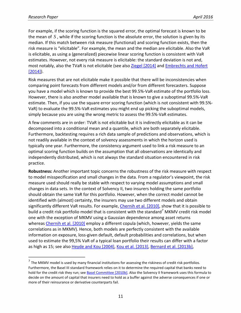
For example, if the scoring function is the squared error, the optimal forecast is known to be the mean of S , while if the scoring function is the absolute error, the solution is given by its median. If this match between risk measure (functional) and scoring function exists, then the risk measure is “elicitable”. For example, the mean and the median are elicitable. Also the VaR is elicitable, as using a (generalized) piecewise linear scoring function is consistent with VaR estimates. However, not every risk measure is elicitable: the standard deviation is not and, most notably, also the TVaR is not elicitable (see also Ziegel [2014] and Embrechts and Hofert [2014]).
Risk measures that are not elicitable make it possible that there will be inconsistencies when comparing point forecasts from different models and/or from different forecasters. Suppose you have a model which is known to provide the best 99.5%-VaR estimate of the portfolio loss. However, there is also another model available that is known to give a suboptimal 99.5%-VaR estimate. Then, if you use the square error scoring function (which is not consistent with 99.5%-VaR) to evaluate the 99.5%-VaR estimates you might end up picking the suboptimal models, simply because you are using the wrong metric to assess the 99.5%-VaR estimates.
A few comments are in order: TVaR is not elicitable but it is indirectly elicitable as it can be decomposed into a conditional mean and a quantile, which are both separately elicitable. Furthermore, backtesting requires a rich data sample of predictions and observations, which is not readily available in the context of solvency assessments in which the horizon used is typically one year. Furthermore, the consistency argument used to link a risk measure to an optimal scoring function builds on the assumption that all observations are identically and independently distributed, which is not always the standard situation encountered in risk practice.
Robustness: Another important topic concerns the robustness of the risk measure with respect to model misspecification and small changes in the data. From a regulator’s viewpoint, the risk measure used should really be stable with respect to varying model assumptions and small changes in data sets. In the context of Solvency II, two insurers holding the same portfolio should obtain the same VaR for this portfolio. However, when the correct model cannot be identified with (almost) certainty, the insurers may use two different models and obtain significantly different VaR results. For example, Chernih et al. [2010], show that it is possible to build a credit risk portfolio model that is consistent with the standard7 MKMV credit risk model one with the exception of MKMV using a Gaussian dependence among asset returns whereas Chernih et al. [2010] employ a different copula (which, however, yields the same correlations as in MKMV). Hence, both models are perfectly consistent with the available information on exposure, loss-given default, default probabilities and correlations, but when used to estimate the 99,5% VaR of a typical loan portfolio their results can differ with a factor as high as 15; see also Heyde and Kou [2004], Kou et al. [2013], Bernard et al. [2013b],
7 The MKMV model is used by many financial institutions for assessing the riskiness of credit risk portfolios. Furthermore, the Basel III standard framework relies on it to determine the required capital that banks need to hold for the credit risk they run; see Basel Committee [2010b]. Also the Solvency II framework uses this formula to decide on the amount of capital that insurers need to hold as a buffer against the adverse consequences if one or more of their reinsurance or derivative counterparts fail.

Research Paper April 2016
12
and Bernard et al. [2015] for more evidence and other examples. In the light of these observations Bernard et al. [2013b] warn for the use of VaR at high confidence levels (e.g., 99.5%) as a basis for capital requirements. Note also that if the external risk measure is not robust, institutions may pursue regulatory arbitrage by choosing a model that significantly reduces the capital requirements or by manipulating the input data.
2. Aggregation and Diversification
2.1 Diversification Benefits and Subadditivity
From the Canadian regulator’s website (OSFI [2014]), one can read “we define risk aggregation as the approach used to calculate the total of each and all of the risk elements. A diversification credit results when the method of aggregation of risks produces results that are less than the sum of the total of the individual risk elements.” Diversification benefits may come from pooling risks within one type of risk such as insurance risk, from pooling several types of risks (e.g., insurance risk and asset risk), across entities or across geographies. There is a careful warning that it is hard to determine the diversification benefits in periods of stress. Capital requirements are determined to cover stress periods and it is especially in these stressed periods that some potential diversification benefits disappear. Reduction of capital should be granted for diversification benefits only in the case when even during stress periods, the diversification benefit stays valid. Some benefits should, however, be recognized. See OSFI [2014] for discussion of diversification benefits between volatility risk and respectively mortality risk, morbidity risk, longevity risk, and lapse risk.
Let us consider portfolios with respective losses 1S and 2S and let 𝜚 be a risk measure used for setting capital requirements; i.e., 𝜚 (𝑆1) is the capital for the first portfolio, 𝜚(𝑆2) is the capital for the second portfolio, and 𝜚(S1 + S2) is the capital of the combined (merged) position. Note that we assume that the losses 1S and 2S do not change nature when merging the portfolios. In reality, however, merging or splitting portfolios may change management, business strategy, and cost structure, among others, and may thus change the marginal distribution of the losses under consideration.
A standard definition for the diversification benefit, denoted by 𝐷𝐷(𝜚, 𝑆1, 𝑆2) is that
𝐷𝐷(𝜚, 𝑆1, 𝑆2) = 𝜚(𝑆1) + 𝜚(𝑆2) − 𝜚(𝑆1 + 𝑆2). (2.6)
Hence, 𝐷𝐷(𝜚, 𝑆1, 𝑆2) provides the gain (loss) one obtains by merging two portfolios. It is clear that if 𝜚 is coherent (and thus subadditive) then the diversification benefit is non-negative, which corresponds to the common intuition that merging risks creates benefits. To confirm this intuition, let us observe that
(𝑆1 + 𝑆2 - 𝜚(𝑆1) - 𝜚(𝑆2))+ ≤ ∑ (𝑆𝑗2𝑗=1 − 𝜚(𝑆𝑗))+. (2.7)
Inequality (2.7) states that the shortfall risk of the merged portfolio is always smaller than the sum of the shortfall risks of the stand-alone portfolios, when the solvency capital requirement is additive. It expresses that, from the viewpoint of the regulator, a merger is beneficial in the sense that shortfall risk decreases when the capitals are summed up. The underlying reason is

Research Paper April 2016
13
clear: within the merged portfolio, the shortfall of one of the entities can be compensated by the gain of the other. In summary, “a merger decreases the shortfall”. Hence, the inequality (2.7) indicates that the solvency capital of the merged position can be smaller than the sum of the solvency capitals of the two stand-alone portfolios. These observations provide support for the common belief that a solvency capital requirement (risk measure) should be subadditive. Indeed, when merging two stand-alone portfolios, subadditivity is allowed by the regulator as long as
(𝑆1 + 𝑆2 - 𝜚(𝑆1 + 𝑆2))+ ≤ ∑ (𝑆𝑗2𝑗=1 − 𝜚(𝑆𝑗))+
holds. In this regard, let us notice that the requirement of subadditivity implies that
(𝑆1 + 𝑆2 - 𝜚(𝑆1 + 𝑆2))+ ≥ (𝑆1 + 𝑆2 - 𝜚(𝑆1) - 𝜚(𝑆2))+, (2.8)
and consequently, for some realizations ),( 21 ss we may have that
(𝑠1 + 𝑠2 - 𝜚(𝑆1 + 𝑆2))+ ˃ (𝑠1 - 𝜚(𝑆1))P
+ + (𝑠2 - 𝜚[𝑆2])+.
Hence, the use of a subadditive risk measure may give rise to a larger shortfall than the sum of the shortfalls of the stand-alone entities, i.e.,
(𝑠1 + 𝑠2 - 𝜚(𝑆1 + 𝑆2))+ ˃ (𝑠1 - 𝜚(𝑆1))P
+ + (𝑠2 - 𝜚(𝑆2))+
may hold (Dhaene et al. [2008]). Therefore, while subadditivity is an acceptable property from the viewpoint of regulators they should restrict the degree of subadditivity in order to avoid that (𝑆1 + 𝑆2 - 𝜚(𝑆1 + 𝑆2))+ becomes too risky as compared to (𝑆1 - 𝜚(𝑆1))+ + (𝑆2 - 𝜚(𝑆2))+.
In this regard, it is also important to note that it is not clear-cut that merging is advantageous for the shareholders. We explain this as follows. For portfolio j (j = 1, 2) the end-of-the-year available funds are given by (𝜚�𝑆𝑗� − 𝑆𝑗)P
+. Indeed, if the loss 𝑆𝑗 is smaller than the capital 𝜚(𝑆𝑗), then the funds that belong to the shareholders (at the end of the reference period) will be given by 𝜚�𝑆𝑗� − 𝑆𝑗, whereas in the case that the loss 𝑆𝑗 exceeds 𝜚(𝑆𝑗), the business unit related to this portfolio gets ruined and the available funds become equal to zero. Since
(𝜚(𝑆1) + 𝜚(𝑆2) - 𝑆1 - 𝑆2)+ ≤ ∑ (𝜚(𝑆𝑗2𝑗=1 ) - 𝑆𝑗)+, (2.9)
we observe that keeping the two portfolios separated might be preferred from the shareholders’ point of view, essentially because in this case firewalls are built in, ensuring that the poor performance of one portfolio will not contaminate the other one. In fact, the shareholders and regulators have interests that are not fully aligned; see also Dhaene et al. [2008] and Dhaene et al. [2009] for more discussion.
2.2 The Fallacy of Using Correlations Only
Some practitioners appear to believe that for aggregating two risks one needs to know only their correlation coefficient. This (wrong) intuition is likely due to the widespread use and importance8 of the multivariate normal distribution that is fully characterized upon 8 The multivariate distribution is at the center of many theories and applications such as linear regression, principal component analysis, CAPM, Markowitz mean-variance analysis, discriminant analysis, capital aggregation (e.g., Basel III and Solvency II), credit portfolio modeling (Moody’s KMV model).

Research Paper April 2016
14
specification of the means, standard deviations, and pairwise correlations (Embrechts et al. [1999, 2002]). However, one should be aware of the fact that the multivariate normal distribution inherits a choice of a specific (Gaussian) dependence already and that correlations are merely needed to parameterize this Gaussian dependence. Effectively, it is easy to construct two normal random variables that have a specific correlation coefficient but that are not jointly (bivariate) normal. To illustrate this feature, let X and Y be standard normally distributed random variables that are independent. In particular, they have a Gaussian dependence with zero correlation. Next, we consider cZ defined as XZ −= if cX |<| and
XZ = if cX |>| 0).>(c It is easy to see that Z is also standard normally distributed: it has perfect positive correlation with X in the tails and perfect negative correlation otherwise. One can then choose ∗c such that correlation between X and ∗c
Z is zero ( 1.538≈∗c ). Hence,
when )(> ∗Φ cp ( )(⋅Φ denotes the c.d.f. of the standard normal random variable),
VaR )(2=)( 1 pZXcp
−∗ Φ+ whereas VaR )(2=)( 1 pYXp
−Φ+ . A numerical illustration can be
found in figure 2.1.
Panel A Panel B Panel C
Figure 2.1: Illustration of three situations where the random variables are standard normally distributed and have zero correlation.
Another example illustrating the deficiencies of correlations concerns risk measurement of a portfolio of credit loans. To explain this idea, let us consider risks iX )1,2,...,=( ni indicating default events so that ni XXXS +++ ...= 2 reflects the number of defaults of the portfolio. Specifically, let ip denote the probability that the i -th company defaults and denote by ijp the pairwise default probability that both company i and company j default. The pairwise default correlation D
ijρ ),1,2,=,( nji 2 is then given as
.)(1)(1
=jjii
jiijDij pppp
ppp−−
−ρ (2.10)
In other words, correlations only reveal full information on interaction between two default events (pairwise), but not really on the manner three or more loans interact. In this regard, note that there is an intrinsic lack of sufficient default statistics (joint defaults are inherently very rare events) and one can simply not expect to be able to reliably estimate higher order joint default probabilities. In other words, assessing the risk of a credit risk portfolio is

Research Paper April 2016
15
inherently subject to model uncertainty9. For example, the influential MKMV model links defaults of companies to the asset return behavior and assumes that asset returns are multivariate normally distributed. This assumption, however, is merely one possible choice and there are no reasons to believe this assumption is close to reality. Bernard, Rüschendorf and Vanduffel [2013b] assess the impact of model uncertainty on VaR calculations. When using
99.5%=p as the basis for calculating VaR and capital requirements (as in Basel III and Solvency II), the results of industry models are typically within a wide range of possible values of VaR. By contrast, model risk appears more limited when using more moderate levels of probability to assessing the VaR. These authors conclude that it might be useful to impose additional constraints on models when used for setting capital requirements. For example, one may use the obtained VaR bounds to set a minimum value on the VaR that is obtained by the internal model, or, one may want to impose a particular model that different institutions need to use for computing capital requirements, as this provides some guarantee that capital levels can be readily compared across institutions also yielding fair competition.
2.3 The Impact of Microcorrelations
In this section, we present another weakness of correlation. Kousky and Cooke [2012] explain how catastrophic risks are usually characterized by fat tails and dependence. With fat-tailed loss distributions, the probability of an event declines only slowly, relative to its severity, meaning that very large losses are not so exceptional (for more mathematical explanations we refer to Kousky and Cooke [2012]). Many natural catastrophes have been shown to be fat tailed. As explained in full detail in Kousky and Cooke [2012], catastrophes can introduce another type of dependence, which is called tail dependence. Tail dependence refers to the probability that one variable exceeds a certain percentile, given that another has also exceeded that percentile. More simply, it means bad things are more likely to happen together. It is clear that a catastrophe will potentially hit simultaneously multiple lines of business for an insurer (houses, cars, health, businesses, etc.). Lescourret and Robert [2006] have observed such tail dependence for lines of insurance covering over 700 storm events in France. Moreover, catastrophic risks tend to be spatially correlated because of the high dependence among the claims due to a given disaster. In practice, this correlation declines with the spatial distance between policies. When it declines to zero, it allows insurers to diversify by holding policies in different regions. Unfortunately, Kousky and Cooke [2012] find that “close to zero” does not count as zero for diversification benefits. Even small, positive, average correlations among policies, which they term “microcorrelations”, can cause problems in risk aggregation.
The main issue with microcorrelation comes from the fact that the law of large numbers fails when risks are not independent even if they display a correlation coefficient that is very close to zero. This is well explained in the works of Kousky and Cooke [2009], Cooke and Kousky [2010], and Cooke et al. [2011] applied on catastrophic risks in Kousky and Cooke [2012]. The basic idea is very simple and is based on the situations in which policies have a small, average, positive correlation (say 0.04, which is the average correlation found in flood insurance claims in the
9 Duffie and Singleton [2012].

Research Paper April 2016
16
U.S. at a county level in Cooke and Kousky [2010]). Cooke and Kousky show how quickly tiny, positive correlations between policies can become pernicious.
Let nXX ,...,1 and nYY ,...,1 be two sets of random variables with the same average variance 𝜎2 and average covariance C (within and between sets). The correlation of the sums of the X ’s and the sum of the Y ’s is easily found to be
CnnnCnYXcorr i
n
ii
n
i 1)(=, 2
2
1=1= −+
∑∑ σ (2.11)
The main issue is that it goes to 1 as n grows, if C is non-zero (even very small), and 2σ is finite. If all variables are independent, then 0=C , and the correlation in (2.11) is zero. To highlight this amplification of correlation, Kousky and Cooke [2009] use flood insurance claim data. They randomly draw pairs of U.S. counties and compute their correlation. The green histogram in figure 2.2 shows 500 such correlations. The average correlation is 0.04. Although a few counties have high and positive correlations, most of the correlations are very small and around zero. Instead of looking at the correlations between two randomly chosen counties, they then sum 100 randomly chosen counties and correlate this with the sum of another distinct set of 100 randomly chosen counties. After repeating this 500 times, they obtain the blue histogram where the average of 500 such correlations (of 100) is 0.23. The red histogram depicts 500 correlations (of 500) with an average value is 0.71. This dramatic increase in correlation is a result of the microcorrelations between the individual variables.
Figure 2.2: Figure 11 from Kousky and Cooke [2009] is reproduced here as an illustration.
2.4 Fitting a Multivariate Distribution
In practice, there exist efficient and accurate statistical techniques to estimate the respective marginal distributions of ),,1 dXX (=X . On the other hand, the joint dependence structure of X is often much more difficult to capture: there are computational and convergence issues with statistical inference of multi-dimensional data, and the choice of multivariate distributions
Research Paper April 2016
17
is quite limited compared to the modelling of marginal distributions. However, an inappropriate dependence assumption can have important risk management consequences. For example, (mis)using the Gaussian multivariate copula can result in severely underestimating probability of simultaneous default in a large basket of firms (McNeil et al. [2010]).
The easiest (and therefore popular) modelling of a multivariate distribution is to use a multivariate Gaussian or multivariate Student distribution. The advantage of the multivariate Student distribution is that it displays some tail dependence. However, there are limitations of this multivariate dependence as there is a single degree of freedom parameter which drives the tail dependence of all pairs of variables.
More generally, multivariate distribution can be decomposed in the marginal distributions iXF ,
di 1,2,...,= (reflecting the stand-alone risks) and a so-called copula function C (reflecting the dependence). More precisely, Sklar [1959]’s theorem states that there exists a vector ( )dUUU ,...,, 21 of standard uniformly distributed random variables such that
)).(),...,(),((= 12
1
211
1 dnXXX
dUFUFUF −−−X (2.12)
where “d= ” reflects equality in distribution. The representation (2.12) thus shows that the
distributional properties of the portfolio X are indeed completely specified by the marginal distributions
iXF )1,2,...,=( di of its risky components and the joint distribution C of
( )dUUU ,...,, 21 describing the interaction among the risks of the portfolio.
Copulas have been extensively studied by Joe [1997] and Nelsen [2007]. There are large families of two-dimensional copulas so that modelling dependence between two variables is relatively easy. The most popular two-dimensional copulas are the Archimedian ones for which an important literature exists on estimation and goodness of fit; see Joe [1997]. Bedford and Cooke [2001, 2002] have then proposed to construct a multivariate copula using pair copulas as building blocks. They also give graphical representations involving a sequence of nested trees, which they call regular vines. This multivariate model, also called pair-copula construction, allows to decompose a complex multivariate model into simpler two-dimensional building blocks. An overview is given by Czado [2010]. This approach is very flexible and allows the dependence between any subset of two variables to be different. For some estimation techniques of parameters of regular vines, one can refer to Kurowicka and Cooke [2006]. An alternative to pair-copula constructions is proposed in Hofert [2012] using hierarchical model; see Okhrin et al. [2013] for estimation issues. The nested Archimedian copulas are studied by Hofert and Pham [2013] and used by Savu and Trede [2010]. A comprehensive overview of dependence in high dimensions can be found in Embrechts and Hofert [2013].
2.5 Summary
Taking into account the dependence among risky components is crucial to assess the aggregate risk of a portfolio. We show that subadditivity of a risk measure is justified from a regulator’s viewpoint. In other words, it is justified that companies receive some diversification benefits when aggregating risks. However, some care is needed: Diversification benefits are often

Research Paper April 2016
18
assessed using correlations, but correlation is a poor measure of dependence. It is merely a single number and not sufficient to describe the complex interaction among risky components. We end section 2 by discussing how to fully describe dependence.
3. Overview of Current Regulation The report of the Basel Committee [2010a] describes the modelling methods used by financial firms and regulators in various countries to aggregate risk. It also aims at identifying the conditions under which these aggregation techniques perform as anticipated in the model and suggests potential improvements. The report expresses doubts about the reliability of internal risk aggregation results that incorporate diversification benefits: “Model results should be reviewed carefully and treated with caution, to determine whether claimed diversification benefits are reliable and robust.” In this section, we very briefly summarize their findings as well as those of other regulators.
3.1 Regulatory Frameworks
Basel III Regulation for Banks. One calculates a bank’s overall minimum capital requirement as the sum of capital requirements for the credit risk, operational risk, and market risk, without recognizing any diversification benefits between the three risk types. The idea that no diversification corresponds to the worst-case situation of the portfolio is not entirely correct. Technically, such property is verified when a coherent risk measure is used but may be violated for other risk measures such as VaR. In other words, it may be possible to aggregate risks so that the VaR of the aggregated risk is higher than the sum of the VaRs.
Within the market risk, banks have the choice between two methods. They may benefit from diversification if they use an internal model approach (IMA). With the standardized measurement method (SMM), the minimum capital requirement for market risk is the sum of the capital charges calculated for each individual risk type (interest rate risk, equity risk, foreign exchange risk, commodities risk, and price risk in options).
Canadian Minimum Capital Test (MCT) and Minimum Continuing Capital and Surplus Requirements (MCCSR). Capital requirements of property and casualty insurers in Canada are based on the MCT. The MCT is a factor-based requirement that aggregates risks as a sum with an explicit credit for diversification between insurance risk and the sum of credit and market risk, so that the total capital required for these risks is lower than the sum of the individual requirements for these risks.
On the other hand, capital requirements of life insurance companies in Canada are computed according to the Office of the Superintendent of Financial Institutions’ (OSFI) MCCSR. The MCCSR employs more sophisticated approaches in some areas. “MCCSR imposes capital requirements for the following risk components: asset default risk, mortality risk, morbidity risk, lapse risk, disintermediation risk, and segregated fund guarantee risk” (Basel Committee [2010a]). Some diversification benefits can be incorporated in the computation of mortality risk, morbidity risk and segregated funds risk but the total MCCSR is calculated as the sum of each risk without potential reduction due to diversification. Again it is (implicitly) assumed here

Research Paper April 2016
19
that this is the worst possible situation. More information on the MCT and MCCSR can be found on the website of OSFI (www.osfi-bsif.gc.ca).
Solvency II. The Solvency Capital Requirement (SCR) under Solvency II is defined as the VaR at 99.5% and a horizon of one year. When aggregating risks, insurers may benefit from diversification: they have the option to use an internal model (without any particular method prescribed) or a standard formula. The standard formula aggregates risks using a correlation matrix (Var-Covar approach) to take into account dependencies.
Swiss Framework for Insurance Companies. Since 2008, all insurers in Switzerland must use the Swiss Solvency Test (SST). Similarly as in Solvency II, there is a standard model and the possibility to use an internal model. The standard model considers the following risks separately: market risk, credit risk (counterparty default), non-life insurance risk, life insurance risk, and health insurance risk. Operational risks do not make part of the current SST. Diversification between risk categories is recognized in all cases. Life insurance companies use the Var-Covar aggregation method, whereas non-life insurers aggregate risks more carefully to find the distribution of the aggregate risk and then use an expected shortfall (or TVaR).
U.S. Insurance Risk-Based Capital (RBC) Solvency Framework. We end our brief review of regulatory frameworks used across the world in the industry by the U.S. RBC. The RBC formula is a standardized system applied to all states in the U.S. and allowing for an easy comparison across companies. Each type of insurer has a separate RBC formula (life, property and casualty, and health). Diversification benefits are incorporated by computing a covariance matrix among the individual risks to reduce the overall capital so that it is smaller than the sums of individual risks.
In the calculation of RBC, the formula is a square root of sum of squares. This amounts to use of a very simple assumption for aggregating risks by assuming that they are fully correlated (correlation equal to one) or independent (zero correlation) (OSFI [2014]).
3.2 Comparison and Comments on International Regulatory Frameworks
Generally, regulatory rules incorporate diversification by taking into account some correlation effect to reduce the total capital (at least in some subcategories). Overall, we observe that regulators all implicitly assume that the sum of the risk numbers is the worst possible situation. “No diversification benefits” is then synonymous to “adding up risk numbers (VaRs)”.
The easiest method to aggregate risks is the Var-Covar approach (which is explicitly mentioned in the Solvency II and SST above and also used by the Australian regulator (OSFI [2014])). It builds on the assumption that the correlation matrix is enough to describe the dependence and that it is possible to aggregate risks based on this correlation matrix. Its strength is in being a simple approach but it is merely only a correct approach for elliptical multivariate distributions such as the Gaussian multivariate distribution. Furthermore, correlation is a linear measure of dependence and does not capture tail dependence adequately. Using such a method to aggregate risk may perhaps be fine to have some idea on the distribution “globally”, but fails when it comes to assessing the risk in the tail, and note that capital requirements are typically based on tail risk measures such as VAR at 99.5%, which essentially reflects the outcome of a 1-in-200 year scenario.

Research Paper April 2016
20
Instead of using the Var-Covar approach, one may use copulas to aggregate the individual risks. This approach is rather flexible and allows one to separate the risk assessment of the marginal distribution of individual risks and their dependence. By specifying a given copula to model some dependence, it is then possible to recognize tail dependence among some risks. However, determining the “right” copula to use is a very hard task that is prone to significant model risk, as we will see later in this report. Statistical methods to fit a multivariate model involve large numbers of parameters and copula families. In addition, understanding the outputs of the model will then require good expertise with the copula approach in order to understand the impact of each assumption made on the dependence. This is a concern and a challenge among institutions.
Another way to capture tail risks and tail dependence is to understand “where the dependence comes from”, and to model the real risk drivers of the dependence among individual risks of the portfolio and understand their interactions. The report of Basel Committee [2010a] suggests using “scenario-based aggregation”. Aggregation through scenarios boils down to determining the state of the firm under specific events and summing profits and losses for the various positions under the specific event. In other words, it means that one needs to incorporate information that one knows about the dependence in some specific states.
We propose in appendix B a method to assess model risk that is somewhat in this spirit, as it allows one to incorporate existing information about the dependence structure among the risks in some states of the world. The scenario-based approach has a clear advantage in that the multivariate model is then based on some clearly identified risk drivers (which can then be simulated, for instance) and it forces the firm to understand the chosen multivariate model: it is no longer a complex set of copulas, but dependence among factors is obtained through reasonable factors. As observed in the report of the Basel Committee [2010a], the results of scenario-based aggregation are easier to interpret with more meaningful economic and financial implications but they require again a deep expertise to identify risk drivers, derive meaningful sets of scenarios with relevant statistical properties, and then use them to obtain a full loss distribution. This will still be a challenging task. A lot of the inputs in these kinds of models come from experts’ judgments. Overall, there is no clear unique solution to solve the problem of risk aggregation. Each method has its pros and cons and may be helpful in given situations and useless in others.
4. Model Risk on Dependence As discussed extensively in the previous sections, one of the main issues in aggregating risks arises from the difficulty in modelling the dependence among a large number of risks, i.e., risk aggregation is prone to model risk. Specifically, we showed in section 1 that there is no unique way to measure risk, and in section 2 that correlation is not enough to measure dependence, and that the full information on dependence contains much more information. However, as it appears in section 3, regulators around the world discuss diversification benefits and propose guidelines in estimating them. But there is no consensus. It turns out that dependence modelling carries a lot of model risk.

Research Paper April 2016
21
In appendices, we provide specific examples that can be helpful in better understanding model risk related to aggregation. Appendix A discusses how to minimize or maximize a given risk measure 𝜚(. ) of the aggregate risk when the distributions of the risky components are known but not their interdependence (consistent with the approach of Embrechts et al. [2013]). This approach is useful to assess model risk on dependence, which is one of the most important factors in assessing aggregated risk.
However, the bounds on model risk on dependence obtained by the approach described in appendix A (see also Embrechts et al. [2013]) are typically too wide to be useful in practice. They ignore all information on dependence and consider only the information about the marginal distributions. There are a few papers studying model risk with partial information on the dependence structure. See among others, Cheung and Vanduffel [2013] for convex ordering bounds with given variance; Embrechts and Puccetti [2006] for bounds on the distribution of S when the copula of X is bounded by a given copula; Tankov [2011] for bounds on S when 𝑛 = 2 and when there are constraints on the copula; Bernard et al. [2013b] when an upper bound on the variance of the aggregate risk is imposed, and Bernard et al. [2014a] when high-order moments are given.
In appendix B, we present a framework which allows practical quantification of model risk (and was developed in Bernard and Vanduffel [2015a]). Importantly, unlike in appendix A, we no longer ignore the available information on dependence. We assume that risk modellers have developed an “as-good-as-possible” multivariate model for a certain portfolio. However, no model is perfect and the extent of misspecification of the proposed model affects the risk measurement and should be assessed. Our framework includes an algorithm allowing actuaries to deal with model risk in a very practical way.
These results make it possible to identify risk measures for which additional information of a well-fitted multivariate model reduces the model risk significantly, making them meaningful candidates for use by risk managers and regulators. Our approach may lead to bounds that are significantly tighter than the (unconstrained) ones available in the literature, accounting for the available information coming from a multivariate fitted model and allowing for a more realistic assessment of model risk. However, model risk remains a significant concern and we recommend caution regarding regulation based on VaR at a very high confidence level since such an assessment is unable to benefit from careful risk management attempts to fit a multivariate model. For instance, we observe from numerical experiments that the portfolio VaR at a very high confidence level (as used in the current Basel regulation) might be prone to such a high level of model risk that, even if one knows the multivariate distribution nearly perfectly, its range of possible values remains wide. In fact, one may then not even be able to reduce the model risk as computed in Embrechts et al. [2013] (see also appendix A) where no information on the dependence among the risks is used at all.
We remark that it could be of interest to consider also a “global” constraint to sharpen the bounds further. A natural global statistic on the distribution of the aggregate risk is the variance and it would be relatively easy to extend our study by using techniques similar to those employed in Bernard et al. [2013b] to account for a maximum possible variance of the aggregate portfolio.

Research Paper April 2016
22
Finally, we assume that the marginal distributions are fixed and known. To capture the possible uncertainty of the marginal distributions, one might consider amplifying their tails. For example, a distortion (Wang transform) could be applied when re-discretizing (instead of using 𝑓𝚤�).
Superadditivity of VaR: We end this section with an important discussion on consequences of aggregation. Specifically, we discuss the superadditivity of VaR. Comonotonicity is the worst-case dependence according to risk-averse decision makers, but that it does not yield the maximum VaR of a portfolio (more details can be found in appendix A). The worst case VaR does not readily occur when the risks are perfectly correlated. As VaR is additive for comonotonic risks, there thus exists a dependence such that
𝑉𝑎𝑅𝑝(𝑋1 + 𝑋2 + ⋯+ 𝑋𝑛) ≥ 𝑉𝑎𝑅𝑝(𝑋1) + 𝑉𝑎𝑅𝑝(𝑋2) + ⋯+ 𝑉𝑎𝑅𝑝(𝑋𝑛) (4.13)
The non-existence of diversification benefits is a situation that is hard to accept by practitioners. In addition, the use of VaR can lead to inconsistent risk rankings since the highest possible value of the risk measure does not correspond to the scenario of full dependence. An important question is when the stated inequality (4.13) is strict, i.e., when does one have (strict) superadditivity and how significant is the superadditivity. It is not difficult to show that one can always find a dependence such that the stated inequality is strict unless 𝑉𝑎𝑅𝑞(𝑋𝑖) is constant for 𝑞 ≥ 𝑝 (see also Bernard, Rüschendorf and Vanduffel [2013b]). This observation allows us to draw the following conclusions:
• When only the marginal distributions are known and the portfolio contains un-bounded risks, then the maximum possible VaR (by finding the worst possible dependence) can be significantly larger than the VaR obtained in the comonotonic case (in which the VaR is additive). For example, Embrechts et al. [2013] show in their figure 5 that for a portfolio of Pareto(2) distributed risks the upper bound on the VaR is about two times larger than the comonotonic VaR (i.e., when the marginal risks are assumed to be comonotonic). See also Embrechts et al. [2014]. More generally, Puccetti and Rüschendorf [2012b] show that under some mild conditions the worst VaR behaves asymptotically as the worst TVaR. The intuition behind this result is as follows. The VaR (measured at some probability level 𝑝) of a comonotonic sum is of course just a particular point on the quantile function of this sum. Now, by changing the comonotonic dependence in the upper tail of the marginal supports (from level 𝑝 onwards), one is able to adjust the upper quantiles of the sum (from level 𝑝 onwards). As the quantile function is non-decreasing, it is then clear that the highest VaR will be obtained if one can change the dependence such that the quantile function of the sum becomes a constant on (𝑝, 1). The constant value is then the maximum VaR and is equal to the comonotonic TVaR (Bernard et al. [2013b]).
Although, the fact that for a given 𝑝, some dependence structures yield a VaR larger than the comonotonic VaR, this may not happen in real-world situations.
• Insurance companies typically have limited liability, hence the VaR cannot be (strictly) superadditive for high levels of probability (which is the standard case for solvency assessments). In fact, in this case, the VaR obtained by using a particular model is likely
Research Paper April 2016
23
to be subadditive. This feature is important, as violation of the subadditivity property is grounds for refuting a risk measure, in particular VaR.
• The situation described above stresses that information on the dependence is crucial if one wants to build models that provide risk numbers that are trustworthy in the sense that upper and lower bounds for these numbers stay in some reasonable range. For example, it might be reasonable to assume that the risks are positively dependent, or the variance of the aggregate risk can be estimated accurately from a statistical analysis of observed losses, or some information on the copula function might be available. In this regard, the results in the literature on ranges of VaR in the presence of additional dependence information are more limited and of an ad hoc nature. Rüschendorf [1991], Embrechts and Puccetti [2010a], and Embrechts et al. [2013] consider the situation in which some of the bivariate distributions are known, and Denuit et al. [1999] study VaR bounds assuming that the joint distribution of the risks is bounded by some distribution. However, the bounds that are proposed in these papers are often hard to deal with, especially for high-dimensional and inhomogeneous portfolios, and they do not necessarily sharpen the unconstrained bounds in a significant way; see also Chernih et al. [2010] for an illustration in the context of credit risk portfolio modelling. These observations, however, contrast with the findings of Bernard et al. [2013b]. They consider the presence of a variance constraint on the portfolio sum as a source of dependence information and show that doing so can significantly tighten the (unconstrained) VaR bounds.
We recall that the risk measure that is dominantly used in regulatory frameworks is VaR. For example, the current European regulation of financial institutions (Basel III) formally relies on the concept of risk-weighted assets (RWA), but is essentially a VaR-based framework. Hence, an approach based on risk-weighted assets may not be appropriate if one needs to aggregate risks to computing VaR of a portfolio. The majority of the academic literature has always argued against the use of VaR because it does not comply with subadditivity. Recently there has been a trend in moving away from VaR and to use TVaR instead; see Embrechts et al. [2014], Basel Committee [2012] and Basel Committee [2013].
5. Conclusions Recent turbulent events such as the subprime crisis, have increased the pressure on regulators and financial institutions to carefully reconsider risk models and to understand the extent to which the outcomes of risk assessments based on these models are robust with respect to changes in the underlying assumptions.
Consequently, we have observed a recent and important literature on risk aggregation and diversification benefits. New approaches for dealing with risk aggregation are to be expected, and the issue of model risk that is inherent in risk aggregation will be the topic of significant study as well.
Section 4 briefly summarized the latest developments on the assessment of model risk. In appendix B, we describe a practical method to assess model risk that takes into account a

Research Paper April 2016
24
typical set of available information. This information may come from statistical modelling such as a multivariate model fitted on the data at hand (and trusted wherever there is enough data) but may also arise from scenarios or experts’ opinions. Assume that some information is known about extreme scenarios. For instance, assume that when one large reinsurer goes bankrupt, then one knows that the insurers that are reinsured by this reinsurer will be subject to losses and thus will all incur losses simultaneously (thus showing a comonotonic situation in the tail). If such information is available, it can be incorporated and it may be possible to reduce the bounds on VaR at high levels.

Research Paper April 2016
25
Appendix A – Model Risk of Dependence when Aggregating Risks
At the 2014 Enterprise Risk Management (ERM) Symposium, the researchers received an award from PRMIA for their paper A New Approach to Assessing Model Risk in High Dimensions dated February 9, 2014. In addition, the researchers published related papers in the Journal of Banking and Finance and in Dependence Modeling. Appendices A and B discuss the approaches for assessing model risk that are included in these papers.
The difficulty in modeling the dependence among a large number of risks is a main issue in aggregating risks, i.e., risk aggregation is prone to model risk. In this appendix, we discuss how to minimize or maximize a given risk measure 𝜚(. ) of the aggregate risk when the distributions of the risky components are known but not their interdependence (consistent with the approach of Embrechts et al. [2013]). In the next section, we will perform the same exercise but by assuming that additional dependence information is available (following the recent method proposed by Bernard and Vanduffel [2015a]).
In what follows, ( )dXXX ,...,,= 21X is the portfolio at hand with given marginal distributions
1XF )1,2,...,=( di and we are interested in the properties of 𝜚(𝑆) where .=1= i
d
iXS ∑ For
convenience, we assume that all means are finite.
Recall from (2.12) that the distributional properties of the portfolio X are completely specified if one also knows the copula that describes the interaction among the risks of the portfolio. In this case, the multivariate distribution of X is known and there is clearly only one possible value for 𝜚(𝑆). However, when the dependence structure is unspecified, 𝜚(𝑆) can take a range of possible values depending on the dependence structure chosen. We aim at finding maximum and minimum possible values for 𝜚(𝑆) reflecting the degree of model risk. It is intuitive that for a strong dependence, 𝑆 becomes a “more variable” risk and 𝜚(𝑆) should be at the highest. Reciprocally, if there is a lot of compensation between the risks then 𝜚(𝑆) should be small. A well-known device to describe the variability among risks is the so-called convex order. Mathematically, the convex10 ordering, ≤ cx� between random variables X , Y is defined as follows
))((�))(( if�cx YfEXfEYX ≤≤
for all convex functions 𝑓(. ) such that the expectation exists. Note that
XXE cx�)( ≤ (A.14)
and also that YX cx≤ implies that X and Y have the same mean but Y has the largest variance. Convex order conforms well with the preferences of risk-averse investors and is very useful to quantify the uncertainty on 𝜚(𝑆). Specifically, when the risk measure 𝜚() is consistent
10 For more details on this ordering in the context of actuarial science, see e.g., Müller and Stoyan [2002], Denuit et al. [2005], Denuit et al. [1999], and Dhaene et al. [2002].

Research Paper April 2016
26
with convex order, then convex order bounds translate into bounds of the risk measure11. This is the case for the variance or the TVaR for instance12. As for the VaR, this risk measure is not consistent with convex ordering as such, but there is still a close relationship between bounds on VaR and convex order bounds as we will also explain hereafter (see also Bernard et al. [2013b]). In any case, it is important to determine upper and lower convex bounds for sums of risks.
A.1 Convex Upper and Lower Bounds
The convex upper bound for a general number 𝑑 of individual risks is attained when the risks are maximally dependent (i.e., co-monotonic) which is an easy way to describe dependence structure. More precisely, in the comonotonic case one actually considers
)),(),...,(),((= 12
1
211
1 nnXXX
dUFUFUF −−−X (A.15)
in which now
.:==...== 21 UUUU n (A.16)
It is intuitively clear that the variables )(= 1 UFX ii− are fully dependent, as they are maximally
increasing in each other. Hence, we obtain that for any portfolio sum iiXS ∑:= in which the
risky components iX are distributed with ,iF
)(�)( 1
1=cxcx UFSSE i
n
i
−∑≤≤ . (A.17)
Proofs for this result (in particular for the second inequality) can be found in many places, the earliest references being Meilijson and Nádas [1979] and Rüschendorf [1982].
While the convex upper bound is straightforward to attain, the stated convex lower bound, i.e., )(SE , is not attainable (sharp) in general. In fact, getting convex lower bounds that are sharp is
a very difficult problem, in particular in higher13 dimensions. Nevertheless, in what follows we show that there exists an algorithm that makes it possible (at least for portfolios with moderate-to-high portfolio size, which is the case of interest) to find a dependence among the risks such that the sum S approximately behaves as the constant ).(SE In other words, the algorithm provides approximations for a convex lower bound of S . Next, we discuss how to
11 Convex order is a natural order in the class of admissible risks. Bernard, Jiang, and Wang [2014b] introduce the concept of admissible risk to describe all possible aggregate risk 𝑆 with given marginal distributions but unknown dependence structure. 12 All concave distortion risk measures are consistent with convex order. 13 For 𝑑 = 2, the convex lower bound is obtained for )(= 1
11 UFX − and )(1= 122 UFX −− as studied by
Denuit et al. [1999] and Tankov [2011], and for 𝑑 ≥ 3 see Bernard et al. [2014b] for some results. In fact, the existence of a sharp lower bound is closely related to the concept of complete mixability (Wang and Wang [2011]) as we explain further in the text; see also Dhaene et al. [2002], Wang and Wang [2011], Embrechts et al. [2013], and Wang et al. [2013] for more background and more mathematical results.

Research Paper April 2016
27
find maximum and minimum risk bounds for portfolios when employing the variance and the VaR as a risk measure.
A.2 Rearrangement Algorithm
The Rearrangement Algorithm (RA) of Puccetti and Rüschendorf [2012a] and further extended in Embrechts et al. [2013] can be seen as a practical method to construct dependence between the variables jX ),,1,2,=( dj 2 such that the portfolio sum dXXS ++ ...= 1 becomes as small as possible in convex order. We recall that this algorithm is important for finding minimum bounds on the variance and TVaR (the maximum bounds are easy to find and follow from comonotonicity in this case), and turns out to be equally important for finding bounds on VaR although VaR does not satisfy convex order.
Without loss of (practical) generality, we assume that the variables jX are discretized and take 𝑛 values that are put in a matrix A randomly14:
.
...
...
...
=
21
22221
11211
ndnn
d
d
xxx
xxxxxx
A (A.18)
The matrix A can be seen as a representation of a possible multivariate structure for ( ).,...,,= 21 dXXXX Importantly, we do not change the respective marginal distributions of 𝑋𝑗
)1,2,...,=( dj by rearranging the outcomes within a column but only the dependence between the 𝑋𝑗s.
1. For 𝑖 from 1 to 𝑑, make the thi column anti-monotonic with the sum of the other columns.
2. Start again from column 1, and make it anti-monotonic with the sums of the columns from 2 to 𝑑.
At each step of this algorithm, we make the −j th column anti-monotonic with the sum of
others, so that the columns, say jX before rearranging and jX~ after rearranging, verify obviously
.~ 1=
+≥
∑∑≠
iji
ji
d
iXXvarXvar
Indeed,
14 For example, we may put in each column of the matrix A the elements in increasing order, in which case we work with a comonotonic structure as the start situation (yielding a portfolio sum that is the largest possible in convex order).

Research Paper April 2016
28
+
∑∑≠
iji
ji
d
iXXvarXvar =
1=
and its minimum when jX is anti-monotonic with ijiX∑≠
. At each step of the algorithm the
variance decreases15, it is bounded from below (by 0) and thus converges to a limit 0≥ (convergence of a monotone sequence of real numbers). If the variance becomes zero, we have found a perfect mixability situation, i.e., the dependence is such that the sum becomes a constant and thus is as convex small as possible (see (A.14)). Otherwise, the algorithm will converge to a local minimum. There is then no guarantee that this minimum is really the minimum of the variance of the sum optimized over all dependence structure, as this minimum may depend on the starting point. However, in practice, it turns out that the convergence is very fast and one typically approximates the situation of complete mixability in a few iterations (unless the portfolio size is very small). In particular, the algorithm works remarkably well for the case of a homogeneous portfolio (in which all jX have the same distribution).
Remark A.1. The algorithm as described above will always stop in a situation where each column is anti-monotonic with the others16.
A.3 Example of Application of the RA
To illustrate the algorithm presented above, we show a very simple example based on a matrix containing eight rows and three columns (i.e., we consider a portfolio containing three risks that take values under eight scenarios) that we report in a matrix similar to the general case given by (A.18)
.
324213101240121230112143
(A.19)
15 Note that the situation in which all of the columns are anti-monotonic with the sum of all others is an obvious necessary condition to have a dependence structure that minimizes the variance. 16 At each step of the algorithm, if a column is not anti-monotonic with the sum of the others, then it is rearranged to make it anti-monotonic. Doing so implies that the variance decreases strictly (as the anti-monotonicity is the unique dependence structure that attains the minimum variance). The matrix has a finite size and therefore there is a finite number of possible rearrangements of this matrix, and therefore the variance can decrease strictly only a finite number of times. If at some point for each column the variance does not change, it means that each column is anti-monotonic with the sum of the others, and therefore the algorithm has stopped.

Research Paper April 2016
29
Here, we start from the comonotonic structure and apply the RA sequentially as described in the above algorithm and we find (i.e., by applying the RA sequentially on the first, second, and third column) that
.
311212204230123140123141
311212104230123240123141
321212104240123230113141
324213101240121230112143
⇒
⇒
⇒
(A.20)
Note that in the last matrix, we find that each column is anti-monotonic with the sum of the two others.
A.4 Model Risk on Dependence on Variance
Proposition A.2 (Bounds on the variance of id
iX∑ 1=
). Let ),...,,( 21 dXXX be a portfolio with
respective marginal distribution .iF Let .=1= i
d
iXS ∑ We have
( ) ( ) ,)(��0=)( 1
1=
≤≤ −∑ UFvarSvarSEvar i
d
i
in which 𝑈 is a random variable that is uniformly distributed on (0,1).
Proposition A.2 is a straightforward consequence of the fact that variance is consistent with convex order and the convex ordering relation (A.17). Hence, the lower bound that we propose here corresponds to the case in which the portfolio sum is constant, i.e., we have the situation of complete mixability as in Wang and Wang [2011]. In this case, we say that the stated lower bound is “sharp”, as there exists a dependence structure among the risks such that the sum is constant and exhibits zero variance exactly. As explained above, the RA attempts to achieve this situation but this is not always possible, in which case the stated lower bound in proposition A.2 is not sharp. In any case, the RA can be seen as a method to get an approximation for the sharp convex lower bound.
Let us illustrate these bounds with the example of eight observations presented above. The maximum variance is obtained when the risks exhibit a comonotonic dependence (see (A.19)) and we find
iX

Research Paper April 2016
30
.
123468911
:=
100110111121222233243344
S
As for the minimum variance, after applying the RA in (A.20) we find as output,
.
55656566
:=
311212204230123140123141
S
We see that the lower bound in proposition A.2 is not attained in this particular case, i.e., there will be no dependence structure among 1X , 2X and 3X such that the sum is constant. However, the output of the RA can still be seen as a very good approximation for the sum that is smallest possible with respect to convex order. In other words, the algorithm makes it possible to find approximate (sharp) lower bounds for the variance.
A.5 Model Risk on Dependence on VaR
As comonotonicity is the worst-case dependence according to risk-averse decision makers, it is intuitive that, similar to the case of the variance, this dependence yields the maximum VaR of a portfolio. We will see, however, that this intuition is wrong in general. Let us first observe that for any sum )(=
1= id
iXS ∑ and 1,<<0 p
( ) ( )SS pp TVaR�VaR ≤ (A.21)
≤ −∑ )(TVaR=� 1
=1UFB i
d
ip . (A.22)
Similarly, one finds that
( )SUFA pi
d
ip VaR�)(LTVaR:= 1
=1≤
−∑ (A.23)

Research Paper April 2016
31
where we have defined the left tail value-at-risk (LTVaR) at level p 1)<<(0 p as
.d][VaR1=)(LTVaR
0uX
pX iu
p
ip ∫ (A.24)
Note that for TVaR and LTVaR,
))(((L)TVaR=)((L)TVaR 11
1=
UFUF ipi
i
d
ip
−− ∑∑
(A.25)
In summary, we then obtain the following result.
Theorem A.3 (Bounds on the VaR of id
iX∑ 1=
). Let ),...,,( 21 dXXX be a portfolio with respective
marginal distribution .iF Let id
iXS ∑ 1=
= and (0,1).∈p Then,
)).((TVaR��))((LTVaR 1
=1=1
1
=1UFXVaRUF iq
n
ii
d
iqiq
n
i
−− ∑∑∑ ≤
≤ (A.26)
These bounds are given and proved in Bernard et al. [2013b]. The question then is if these bounds can be sharp. To deal with this problem let us note that
.)(�)( 1
=1
1
=1
≤
−− ∑∑ UFTVaRUFVaR i
d
ipi
d
ip (A.27)
Hence, in order to attain the upper bound 𝐷, the idea is to start with the comonotonic dependence and next change it such that the inequality (A.26) turns into an equality. As 𝑇𝑉𝑎𝑅𝑝 is the average of all upper 𝑉𝑎𝑅𝑞s on the interval [𝑝, 1], it is clear that the equality is obtained if
the VaR of the comonotonic sum )(11=
UFid
i−∑ becomes constant on [𝑝, 1] (by changing this
comonotonic dependence). Let iG denote the distribution of iF when restricted17 to the upper 𝑝-part of iF . In order to attain the upper bound, one thus needs to find a dependence between the risks (now with marginal distributions iG ) such that the corresponding sum becomes constant (i.e., the risks are completely mixing). In general, the mixing property does not hold and the stated bounds are thus not sharp. However, it is now clear that (approximations of) sharp VaR bounds are obtained by finding a dependence between the risks (with marginal distributions iG ) such that the corresponding sum becomes as convex small as possible (see also Bernard et al. [2013b]). A similar reasoning shows that in order to reach the stated lower bound as closely as possible, one should change the comonotonic dependence such that the quantile function of the comonotonic portfolio sum becomes as flat as possible on the interval
].[0, p
We build on this idea to propose a practical algorithm to approximate sharp bounds. Hence, let us show how to find approximate sharp bounds with the discrete example discussed above
17 Formally, iG is the distribution of )(1 VFi
− , where V is uniformly distributed on ,1].[q

Research Paper April 2016
32
when the level 𝑝 used to assess the VaR is 5/8. Note that we start from the comonotonic structure in the matrix.
.233243344
100110111121222233243344
⇒
We then apply the RA in the three corresponding rows.
.343243234
243243334
233243344
⇒
⇒
So that the sums are respectively 9, 9 and 10 and thus the maximum VaR is 9. To obtain the minimum VaR, one works on the lower values of each 𝑋𝑖 and applies the RA on these values
.
100110111121222
100110111121222233243344
⇒
Applying the RA as described above
.
120120111111202
100110111121222
⇒
so that the values of the sums are 4,3,3,3, and 3. Therefore the minimum VaR is 4.

Research Paper April 2016
33
Appendix B – Model Risk of Dependence when Aggregating Risks and Model Risk Quantification
In this appendix, we present a framework which allows practical quantification of model risk (and was developed in Bernard and Vanduffel [2015a]). We assume that risk modellers have developed an “as-good-as-possible” multivariate model for a certain portfolio ),...,,( 21 dXXX . However, no model is perfect and we want to assess to what extent misspecification of the proposed model affects the risk measurement of .= ii
XS ∑ Importantly, unlike in appendix A,
we no longer ignore the available information on dependence. Our framework includes an algorithm allowing actuaries to deal with model risk in a very practical way, as we will show in full detail.
These results make it possible to identify risk measures for which additional information of a well-fitted multivariate model reduces the model risk significantly, making them meaningful candidates for use by risk managers and regulators. For instance, we observe from numerical experiments that the portfolio VaR at a very high confidence level (as used in the current Basel regulation) might be prone to such a high level of model risk that, even if one knows the multivariate distribution nearly perfectly, its range of possible values remains wide. In fact, one may then not even be able to reduce the model risk as computed in Embrechts et al. [2013] (see also appendix A) where no information on the dependence among the risks is used at all.
The idea pursued in our approach is intuitive and corresponds to real-world situations. Let us assume that we have observed 𝑁 𝑑-dimensional vectors of observations Nidii xx 1,...,=1 )},...,{( and that a multivariate model has already been fitted to this data set. In other words, there is a joint distribution of ),...,,( 21 dXXX available (benchmark model). However, we are aware that the model is subject to misspecification, especially due to lack of data. Hence, we split ℝ𝑑 into two subsets: ℱ will be referred to as the “fixed” or “trusted” area and 𝒰 as the “unfixed” or “untrusted” area. 𝒰 reflects the area in which the data are not considered trustworthy (rich) enough to conclude that the fitted model is appropriate (in that area). Note that
ℝ𝑑 = ℱ ∪ 𝒰.
If one has perfect trust in the model, then all observations reside in the “trusted” part (𝒰=∅) and there is no model risk. On the contrary, ℱ = ∅ when there is no trust in the fit of the dependence, which corresponds to the case studied by Embrechts et al. [2013] (see also appendix A).
A closely related problem has already been studied for two-dimensional portfolios (𝑑 = 2) when some information on the dependence (copula) is available; see for example Tankov [2011], Bernard et al. [2012], and Bernard et al. [2013a]. Tankov [2011] uses extreme dependence scenarios to find model-free bounds for the prices of some bivariate derivatives, whereas Bernard et al. [2014] and Bernard et al. [2014]18 use such scenarios to determine optimal investment strategies for investors with state-dependent constraints. While both applications show that finding bounds on copulas in the bivariate case can be of interest, risk 18 This paper received the 2015 Redington prize from the SOA.

Research Paper April 2016
34
management typically involves more than two risks. Unfortunately, finding bounds on copulas in the general 𝑑−dimensional case in the presence of constraints is not only more difficult but also less useful for risk management applications. The reason is that when 𝑑 > 2, in most cases, the worst copula (under constraints) of a vector ),...,,( 21 dXXX does not give rise to the
highest possible value of the risk measure at hand of ,=1= i
d
iXS ∑ because the marginal
distributions also have an impact; see e.g., Bernard et al. [2014b] for illustrations of this feature.
In addition, there are very few papers in the literature that deal explicitly with high-dimensional problems and the presence of (partial) information on the dependence structure: Rüschendorf [1991], Embrechts and Puccetti [2010b], and Embrechts et al. [2013] consider the situation in which some of the bivariate distributions are known, Denuit et al. [1999] study VaR bounds assuming that the joint distribution of the risks is bounded by some distribution; and Bernard et al. [2013b] compute VaR bounds when the variance of the sum is known. They are able to show how the information on the variance of the aggregate risk allows one to reduce the distance between the maximum VaR and the minimum VaR significantly. Moreover, they provide an algorithm (extended RA) that can be used by actuaries to assess VaR bounds (and thus model risk on VaR assessment) in a very practical way when only the variance of the aggregate risk is known.
The set-up in all of these papers is sometimes hard to reconcile with the information that is available in practice; or, it does not make use of all available dependence information. Furthermore, while the bounds that are proposed in these papers might be sharp (attainable), they are often hard to compute numerically, especially for higher dimensions with inhomogeneous risks. Note also that the bounds obtained do not always make it possible to strengthen the unconstrained bounds in a significant way, suggesting that additional dependence information is needed in order to obtain better bounds; see also Wang and Wang [2011], Embrechts et al. [2013], Wang et al. [2013], and Bernard et al. [2014b] for related results.
Hence, in this final section, we study bounds for risk measures of the aggregate risk 𝑆 by using information on the multivariate joint distribution of its components 𝑋𝑖 (which embeds information on the dependence) rather than using copula information. We propose two methods for deriving bounds on risk measures. The first method could be non-parametric, it builds on the RA of Embrechts et al. [2013] and allows one to find sharp bounds. The second method provides analytic, simple bounds but may not be sharp. In practice, we also show through examples that analytical bounds are close to being sharp.
The outline of this section is as follows. First, we present the practical method using the RA (section B.3). This method can be performed directly using the data at hand (without fitting a model), so that in this case, model risk can be assessed in a fully non-parametric way. This method builds on the rearrangement algorithm that was recently developed by Puccetti and Rüschendorf [2012a] and further studied by Embrechts et al. [2013]. It relies on a discretized version of the problem described above and uses a matrix representation to approximate the worst-case dependence structures. We then give the analytical form and illustrate it by

Research Paper April 2016
35
simulations of N(0,1) risks and Pareto risks in section B.4. We provide bounds that can be computed directly (using, for instance, Monte Carlo simulations) but that may not be sharp. Our numerical results indicate that in high dimensions the bounds computed using the direct method in section B.4 are close to the non-parametric bounds as computed in section B.3. In other words, while finding sharp bounds is theoretically a difficult problem, the numerical illustrations suggest that the algorithm that we propose in section B.4 leads to nearly sharp bounds. The numerical results also show that the new bounds typically outperform the (unconstrained) ones already available in the literature and thus allow for more realistic assessment of model risk. However, model risk remains a significant concern, especially when using a risk measure that focuses on “tail-type” events, such as the VaR.
B.1 Theoretical Setting and Assumptions
Let ),...,,( 21 dXXX be some random vector of interest. Let ℱ ⊂ ℝ𝑑 and 𝒰 = ℝ𝑑\ℱ. We assume that we know
i. the marginal distribution iF of iX on ℝ for 𝑖 = 1, 2, … ,𝑑;
ii. the distribution of ),...,,( 21 dXXX | { ),...,,( 21 dXXX ∈ ℱ}; and
iii. the probability ∈),...,,((:= 21 df XXXPp ℱ), as well as 𝑝𝑢 := P((𝑋1,𝑋2, … ,𝑋𝑑 ∈ 𝒰) =1 − 𝑝𝑓 .
The joint distribution of ),...,,( 21 dXXX is thus not completely specified (unless ℱ = ℝ𝑑 and
𝒰 = ∅). Consequently, risk measures (e.g., the VaR) of the aggregate sum id
iX∑ 1=
cannot be
computed precisely. In fact, there are many vectors ),...,,( 21 dYYY that agree with ),...,,( 21 dXXX for the properties (i), (ii), and (iii) but have a different risk measure of their
sum. In what follows, we are interested in finding the extreme possible values of the risk measure at hand, as the gap between the minimum and the maximum can be useful in measuring model risk. Formally, we use the following definition of model risk. This definition is in the same spirit as in Barrieu and Scandolo [2015].
Definition B.1 (Model risk). Let ),...,,( 21 dXXX be a random vector satisfying (i), (ii), and (iii)
and assume that one uses a (law-invariant) risk measure 𝜚(. ) to assess the risk of id
iX∑ 1=
.
Define
where the supremum and the infimum are taken over all other (joint distributions of) random vectors ),...,,( 21 dYYY that agree with (i), (ii), and (iii). The model risk that one underestimates the risk by computing a direct estimate of 𝜚(∑𝑋𝑖) in some chosen benchmark model (i.e., when some multivariate distribution for ),...,,( 21 dXXX has been specified) is defined as

Research Paper April 2016
36
(B.28)
and, similarly, the model risk for overestimation is given as
(B.29)
The rest of this section aims at obtaining the maximum and minimum possible values 𝜚ℱ+ and 𝜚ℱ− of 𝜚(∑ 𝑋𝑖𝑑
𝑖=1 ). The recent literature on model risk estimation has dealt mainly with the case in which there is full uncertainty on the dependence among the risks iX ),1,2,...,=( di i.e., when ℱ = ∅ (Appendix A where we reviewed the work of Embrechts et al. [2013] with respect to VaR. See also Bernard et al. [2014b] regarding a convex risk measure). In this section, we consider the case in which information on the dependence translates into joint distributions that are partially known.
In this respect, it will be useful to consider the indicator variable 𝕀 corresponding to the event “ ),...,,( 21 dXXX ∈ ℱ”
(B.30)
so that one can express the probabilities that a random vector takes values in ℱ resp. in 𝒰 as
(B.31)
Let us also introduce a standard uniformly distributed random variable 𝑈 independent of the event “ ),...,,( 21 dXXX ∈ ℱ” (and thus also independent of 𝕀) as well as a random vector
),...,,( 21 dZZZ defined by
(B.32)
where 1),...,2,1(|
−∈UdXXXiXF denotes the (left) inverse of the distribution function
Note that )(1
),...,2,1(| xFdXXXiX
−∈U can be computed, as the marginal distribution of iX is known and
the joint distribution of ),...,,( 21 dXXX is known on ℱ (see the properties (i) and (ii)). Further, all iZ )1,2,...,=( di are increasing in the (common) variable 𝑈, and thus ),...,,( 21 dZZZ is a comonotonic vector with known joint distribution. Define also
(B.33)
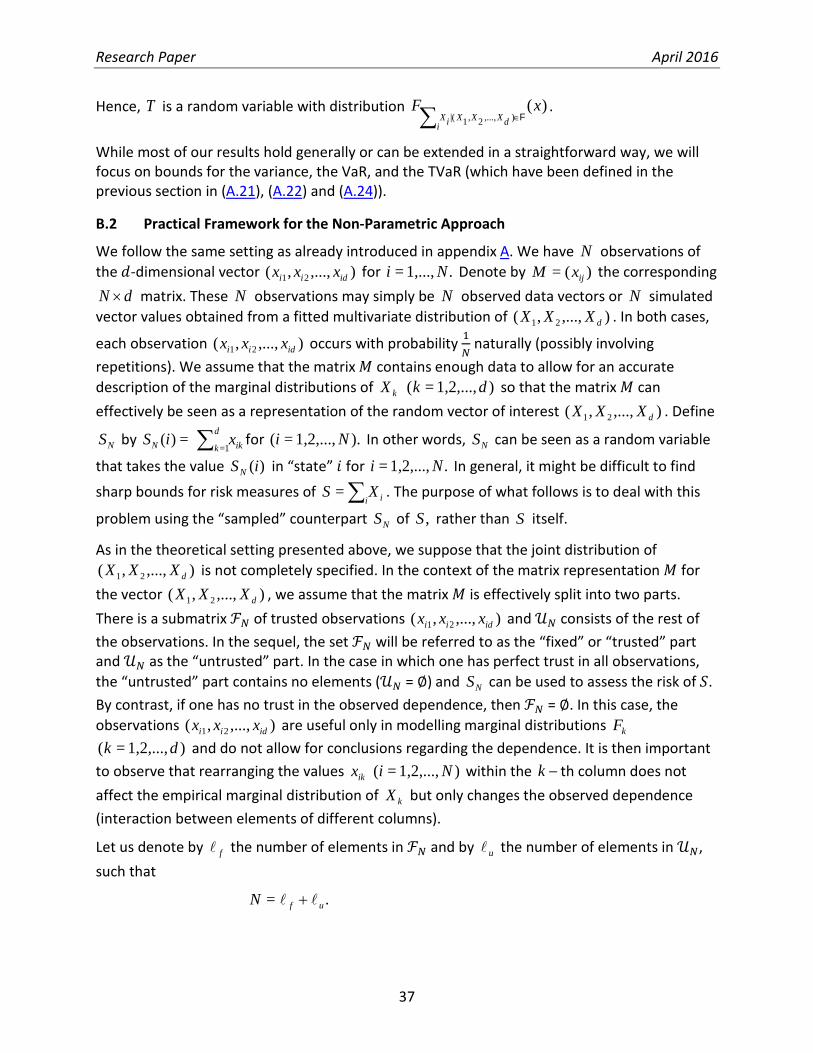
Research Paper April 2016
37
Hence, T is a random variable with distribution )(),...,2,1(|
xFdXXXiX
iF∈∑ .
While most of our results hold generally or can be extended in a straightforward way, we will focus on bounds for the variance, the VaR, and the TVaR (which have been defined in the previous section in (A.21), (A.22) and (A.24)).
B.2 Practical Framework for the Non-Parametric Approach
We follow the same setting as already introduced in appendix A. We have N observations of the 𝑑-dimensional vector ),...,,( 21 idii xxx for .1,...,= Ni Denote by )(= ijxM the corresponding
dN × matrix. These N observations may simply be N observed data vectors or N simulated vector values obtained from a fitted multivariate distribution of ),...,,( 21 dXXX . In both cases,
each observation ),...,,( 21 idii xxx occurs with probability 1𝑁
naturally (possibly involving repetitions). We assume that the matrix 𝑀 contains enough data to allow for an accurate description of the marginal distributions of kX )1,2,...,=( dk so that the matrix 𝑀 can effectively be seen as a representation of the random vector of interest ),...,,( 21 dXXX . Define
NS by =)(iSN ikd
kx∑ 1=
for ).1,2,...,=( Ni In other words, NS can be seen as a random variable
that takes the value )(iSN in “state” 𝑖 for .1,2,...,= Ni In general, it might be difficult to find
sharp bounds for risk measures of iiXS ∑= . The purpose of what follows is to deal with this
problem using the “sampled” counterpart NS of ,S rather than S itself.
As in the theoretical setting presented above, we suppose that the joint distribution of ),...,,( 21 dXXX is not completely specified. In the context of the matrix representation 𝑀 for
the vector ),...,,( 21 dXXX , we assume that the matrix 𝑀 is effectively split into two parts. There is a submatrix ℱ𝑁 of trusted observations ),...,,( 21 idii xxx and 𝒰𝑁 consists of the rest of the observations. In the sequel, the set ℱ𝑁 will be referred to as the “fixed” or “trusted” part and 𝒰𝑁 as the “untrusted” part. In the case in which one has perfect trust in all observations, the “untrusted” part contains no elements (𝒰𝑁 = ∅) and NS can be used to assess the risk of 𝑆. By contrast, if one has no trust in the observed dependence, then ℱ𝑁 = ∅. In this case, the observations ),...,,( 21 idii xxx are useful only in modelling marginal distributions kF
)1,2,...,=( dk and do not allow for conclusions regarding the dependence. It is then important to observe that rearranging the values ikx )1,2,...,=( Ni within the −k th column does not affect the empirical marginal distribution of kX but only changes the observed dependence (interaction between elements of different columns).
Let us denote by f the number of elements in ℱ𝑁 and by u the number of elements in 𝒰𝑁, such that
.= ufN +
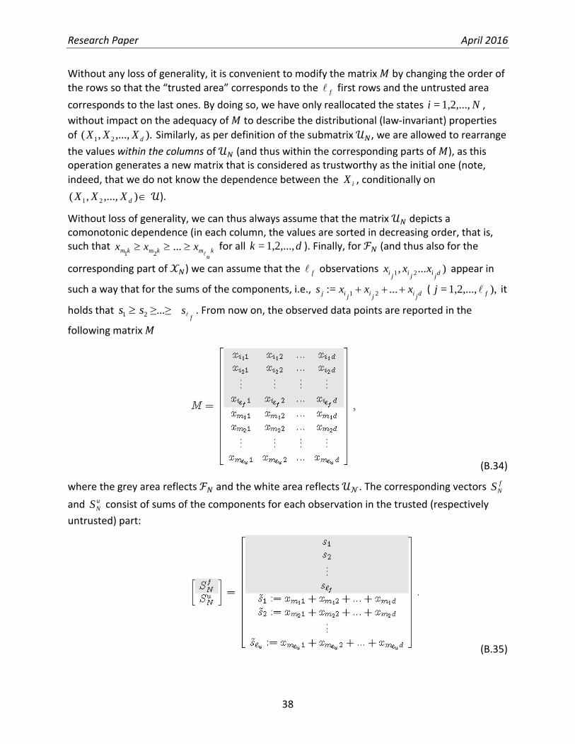
Research Paper April 2016
38
Without any loss of generality, it is convenient to modify the matrix 𝑀 by changing the order of the rows so that the “trusted area” corresponds to the f first rows and the untrusted area corresponds to the last ones. By doing so, we have only reallocated the states Ni 1,2,...,= , without impact on the adequacy of 𝑀 to describe the distributional (law-invariant) properties of ).,...,,( 21 dXXX Similarly, as per definition of the submatrix 𝒰𝑁, we are allowed to rearrange the values within the columns of 𝒰𝑁 (and thus within the corresponding parts of 𝑀), as this operation generates a new matrix that is considered as trustworthy as the initial one (note, indeed, that we do not know the dependence between the iX , conditionally on
∈),...,,( 21 dXXX 𝒰).
Without loss of generality, we can thus always assume that the matrix 𝒰𝑁 depicts a comonotonic dependence (in each column, the values are sorted in decreasing order, that is, such that k
umkmkm xxx
≥≥≥ ... 21
for all dk 1,2,...,= ). Finally, for ℱ𝑁 (and thus also for the
corresponding part of 𝒳𝑁) we can assume that the f observations )..., 21 djijiji xxx appear in
such a way that for the sums of the components, i.e., djijijij xxxs +++ ...:= 21 ( ),1,2,...,= fj it
holds that ≥1s 2s ≥...≥f
s . From now on, the observed data points are reported in the
following matrix 𝑀
(B.34)
where the grey area reflects ℱ𝑁 and the white area reflects 𝒰𝒩. The corresponding vectors fNS
and uNS consist of sums of the components for each observation in the trusted (respectively
untrusted) part:
(B.35)

Research Paper April 2016
39
While 1s ≥ 2s ≥...≥f
s are trusted, the sums is~ change when the choice of dependence in 𝒰𝑁
is varied. In fact, the set },...,{ 1 fii can be seen as the collection of states (scenarios) in which
the corresponding observations are trusted, whereas the set },...,{ 1 umm provides the states in
which there is doubt with respect to the dependence structure.
For pedagogical purposes, we now provide a simple example of this set-up. It will be used throughout this section to illustrate each algorithm that we propose. This toy example is not meant to represent a realistic set of observations since, in true applications, there would be a large number of observations (here 𝑁 = 8) and possibly a large number of variables (here
)3=d . The eight observations are given as follows, with three observations trusted ( 3=f ), which appear in the grey area of the matrix:
(B.36)
Without loss of generality we can then consider for further analysis the following matrix 𝑀 and the vectors of sums f
NS and uNS , as follows:
(B.37)
Finally, with some abuse of notation (completing by 0 so that fNS and u
NS take eight values), one also has the following representation of NS :
NS = 𝕀𝑆𝑁𝑓 + (1 − 𝕀)𝑆𝑁𝑢, (B.38)
where 𝕀 =1 if ),...,,( 21 idii xxx ∈ ℱ𝑁 ).1,2,...,=( Ni In fact, fNS can be readily seen as the sampled
counterpart of the 𝑇 that we used previously (see definition B.33), whereas uNS is a
comonotonic sum and corresponds to the sampled version of id
iZ∑ 1=
. In this last section, we
aim at finding worst case dependence structures allowing for a robust risk assessment of the portfolio sum 𝑆 (𝑆𝑁). This amounts to rearranging the outcomes in the columns of the

Research Paper April 2016
40
untrusted part 𝒰𝑁 such that the risk measure at hand for NS becomes maximized (resp. minimized).
B.3 Bounds on a Given Risk Measure
In this section, we discuss the sharpness19 of upper and lower bounds for the three risk measures defined earlier, namely the variance, TVaR, and VaR.
We discussed analytical bounds and sharpness of these bounds in the previous section, and in particular in proposition A.2 that gives unconstrained bounds for variance, and in proposition A.3 that gives unconstrained bounds for VaR. They can be naturally extended to the case under study here with constraints.
B.3.1 Theoretical Bounds on Variance and Tail Value-at-Risk
The next proposition gives easy-to-compute upper and lower bounds for the variance of a portfolio sum i
d
iX∑ 1=
.
Proposition B.2 (Bounds on the variance of id
iX∑ 1=
). Let ),...,,( 21 dXXX be a random vector
that satisfies properties (i), (ii), and (iii), and let 𝕀 and ),...,,( 21 dZZZ be defined as in (B.30) and (B.32). We have
The proof of proposition B.2 can be found in Bernard and Vanduffel [2015a]. The stated upper and lower bounds in proposition B.2 are intuitive and extend proposition A.2 in a natural way. When computing the variance of the portfolio sum i
d
iX∑ 1=
, one needs to consider the events
),...,,( 21 dXXX ∈ ℱ and ),...,,( 21 dXXX ∈ 𝒰 separately. The distribution of id
iX∑ 1=
is known
on the event { ),...,,( 21 dXXX ∈ ℱ} , but unknown on the event { ),...,,( 21 dXXX ∈ 𝒰}. On 𝒰,
one then substitutes sum iiX∑ by the constant )( ii
ZE∑ (to compute the lower bound and
thus to minimize variance) and by the comonotonic sum iiZ∑ (to compute the upper bound
and thus to maximize variance). Note in particular that when 𝒰 = ∅, the upper bound is equal to the lower bound and there is no model risk.
Next, we discuss bounds for the TVaR as they are similar to the variance (because both measures are consistent with convex order).
Proposition B.3 (Bounds on the TVaR of ∑ =
d
1i iX ). Let ),...,,( 21 dXXX be a random vector that
satisfies properties (i), (ii), and (iii), and let 𝕀 and ),...,,( 21 dZZZ as defined in (B.30) and (B.32). We have that 19 Recall that a bound on a risk measure is “sharp” if there exists a dependence structure among the risks such that this bound is attained.

Research Paper April 2016
41
There is no model risk (the bounds reduce to the same value) when 𝒰 = ∅.
Some of the bounds stated in propositions B.2 and B.3 can be sharp. In particular, the upper bounds for the variance and for the TVaR stated in propositions B.2 and B.3 are sharp, without further conditions. Note, indeed, that the multivariate vector
(B.39)
satisfies conditions (i) and (ii). In contrast, the stated lower bounds may not be sharp because 𝕀𝑋𝑖 + (1 − 𝕀)𝐸(𝑍𝑖) is usually not distributed with iF ).1,2,...,=( di In order to get close to the stated lower bounds, one should try to modify the dependence of the vector ),...,,( 21 dZZZ such that dZZZ +++ ...21 becomes constant (and thus equal to ))(...)()( 21 dZEZEZE +++ . We use this insight to propose an algorithm below that makes it possible to approximate the sharp bounds when the risk measure used is the standard deviation or the TVaR.
B.3.2 Practical Bounds on Standard Deviation and TVaR
From proposition B.2 it is clear that in order to maximize the variance of NS one needs a comonotonic scenario on 𝒰𝑁. However, we have already initialized a comonotonic structure (without loss of generality), and the corresponding values of the sums are exactly the values is~
)1,2,...,=( ui reported for uNS in (B.35). The upper bound on variance is then computed as
,)~()(1 2
1=
2
1=
−+− ∑∑ ssss
N i
u
ii
f
i
(B.40)
where the average sum s is given by
.~1=1=1=1=1=1=
+∑∑∑∑ i
u
ii
f
iij
d
j
N
iss
Nx
Ns
(B.41)
To achieve the minimum variance bound found in proposition B.2, the values of uNS must be as
close as possible to each other; ideally, uNS must be constant. In this regard, the concept of
complete mixability appears as a theoretical device. “Complete mixability” refers to the dependence structure that makes the sum u
NS constant (Wang and Wang [2011]). To make this the case, in practice, we apply the rearrangement algorithm of Embrechts et al. [2013] to the matrix 𝑈𝑁 (untrusted part) to render it as close as possible to the complete mixability condition. For completeness, the algorithm is presented in section A.2. Denote by m
is~ the corresponding values of the sums of u
NS after applying the RA. We then compute the minimum variance as follows:

Research Paper April 2016
42
,)~()(1 2
1=
2
1=
−+− ∑∑ ssss
Nm
i
u
ii
f
i
(B.42)
where s is computed as in (B.41).
We illustrate the upper and lower bounds (B.40) and (B.42) for the variance derived above with the matrix 𝑀 of observations provided in (B.37). We then use the comonotonic structure for the untrusted part of the matrix 𝑀 and compute the vectors of sums f
NS and uNS as defined
above in (B.37). The average sum is s = 5.5. The maximum variance is equal to
8.75.)~()(81 2
5
1=
23
1=
≈
−+− ∑∑ ssss c
ii
ii
For the lower bound, we apply the RA to the 𝑈𝑁 and we obtain
(B.43)
With an average sum 5.5=s , the minimum variance can be calculated as
2.5.)~()(81 2
5
1=
23
1=
≈
−+− ∑∑ ssss m
ii
ii
Assume that we want to fix the TVaR at probability level 𝑝, so that, for ease of exposition,
),(1:= pNk − (B.44)
where 𝑘 is an integer. Similarly to the case of maximizing the variance, it follows from proposition B.3 that in order to obtain the maximum TVaR one needs a comonotonic scenario on 𝒰𝑁. Hence, we merely need to select the 𝑘 highest values from f
NS and uNS as computed in
(B.35). Let us label these values by ∗1s , ∗
2s ,..., ∗ks (ranked in decreasing order), and we can then
easily compute the maximum TVaR at probability level 𝑝. Also, the minimum TVaR is obtained similarly to the minimum variance. First, apply the RA to the untrusted part of the matrix 𝑈𝑁 to render the variance of the (new) sum u
NS as small as possible. Then, select the 𝑘 highest values
out of fNS and u
NS , say: ∗1s , ∗
2s ,..., ∗ks (ranked in decreasing order) and compute the minimum
TVaR.
Let us consider the previous example again. Let us choose 𝑝 = 5/8, so that 𝑘 = 3. The highest 𝑘 = 3 values are 8, 8 and 10 and the maximum TVaR is then 26/3 (≈ 8.67). After application of

Research Paper April 2016
43
the RA, we obtain (B.43) for uNS and thus the highest three outcomes that we observe for u
NS and f
NS are 8, 8 and 5. Hence, the minimum TVaR is 21/3 = 7.
B.3.3 Theoretical Bounds on Value-at-Risk
VaR is a widely used risk measure in financial services. The following proposition provides bounds on VaR.
Proposition B.4 (VaR Bounds for ∑=
d
i iX1
). Let ),...,,( 21 dXXX be a random vector that satisfies
properties (i), (ii), and (iii), and let 𝕀, ),...,,( 21 dZZZ and 𝑈 be defined as in (B.30) and (B.32). Define the variables iL and iH as
( ) ( )iUiiUi ZTVaRHZLTVaRL = and =
and let
Bounds on the VaR of the aggregate risk are given as
.��1=
pi
d
ipp MXVaRm ≤
≤ ∑ (B.45)
The proof can be found in Bernard and Vanduffel [2015b]. Initially, the appearance of variables iL and iH may seem somewhat odd. However, note that the variables ,iZ which played
crucial roles in propositions B.2 and B.3, can also be expressed as ( ),= iUi ZVaRZ and here we merely use ( )iU ZTVaR and ( )iU ZLTVaR instead. Thus, proposition B.4 has a similar form20 to that of proposition B.3 resp. B.2, but the bounds proposed are usually not sharp21. We observe that in the case of no uncertainty (i.e., 𝒰 = ∅) there is no model risk, as 𝕀 = 1. When there is full uncertainty, i.e., 𝒰 = ℝ𝑑, then 𝕀 = 0, and we are returned to the unconstrained lower bound on the VaR of a portfolio given in proposition A.3 (see also theorem 2.1 of Bernard, Rüschendorf, and Vanduffel [2013b]). Note also that the VaR bounds are not sharp in general.
For practical calculations it might be convenient to use an alternative formulation of the stated VaR bounds.
Proposition B.5 (Alternative formulation of the VaR Bounds). Let ),...,,( 21 dXXX be a random vector that satisfies properties (i), (ii), and (iii), and let 𝕀, ),...,,( 21 dZZZ and 𝑇 be defined as in (B.30), (B.32) and (B.33). Recall that 𝑝𝑓 = 𝑃(𝕀 = 1). Define
20 Note that VaR is not consistent with convex order, although there are some connections (see Bernard et al. [2013b] and Bernard et al. [2012]). 21 Note, indeed, that the variables iH and iL are not distributed as (𝑋𝑖|𝕀 =0).

Research Paper April 2016
44
,)(|),(inf:==1
1
21
≥∈ ∑
−
−∗ i
d
ifpfpp ZTVaRTVaR aaaaaa
where
−+
f
f
ppp 1
0,max=1a and
fpp1,min=2a . Then, for 𝑝 ∈ (0, 1),
(B.46)
The expressions for the lower bound 𝑚𝑝 are obtained by replacing, in the above statements, TVaR with LTVaR.
The proof of proposition B.5 is provided in the appendix of Bernard and Vanduffel [2015a]. We can illustrate proposition B.5 in a discrete setting, in which the probability space Ω has 𝑁 states. Assume that the event { ),...,,( 21 dXXX ∈ ℱ} corresponds to the set },,...,{ 1 f
ωω whereas
),...,,({ 21 dXXX ∉ ℱ} corresponds to the set },...,{ 1 uff ++ ωω with Nuf = + (𝑁 is the
number of states). Then, N
p ff
= and
Np u
u= . Assume that i
d
iZ∑ 1=
takes u values
,~...~~21 u
sss ≥≥≥ and that 𝑇 then takes f values f
sss ≥≥≥ ...21 . Specifically, assume
𝑁 = 8, 3=f , 5=u , 𝑠1 = 8 ≥ 𝑠2 = 8 ≥ 𝑠3 = 3 and
1=~3=~4=~7=~10=~54321 sssss ≥≥≥≥ , 3/8=fp and 5/8=up . For 𝑝 = 5/8, we apply (B.46) in
proposition B.5 and find that 0.75=∗a and that the maximum VaRp is equal to 8=)(0.55 iZTVaR ∑ . These values will be confirmed by the algorithm described below.
B.3.4 Practical Bounds on VaR
To compute the maximum VaR, we present an algorithm that can be applied directly to the matrix 𝑀of the observed data, and thus leads to non-parametric bounds on the VaR. Recall that the first f rows of matrix 𝑀 correspond to ℱ𝑁, whereas u denotes the number of rows of
𝒰𝑁 (N = f + u ). In the algorithm, we also make use of fNS and u
NS , which we treat as random variables. To compute the VaR at probability level 𝑝, we define
)(1:= pNk − (B.47)
where we assume that 𝑘 is an integer.
The algorithm is based on proposition B.5 and on the following motivation. Recall from the discussion of proposition B.4 that the stated upper and lower VaR bounds are not sharp in general. Nevertheless, we are able to propose an algorithm to approximate sharp bounds. We explain this idea further. Hence, let 𝑝 ∈ (0, 1) and let us observe that, almost surely,

Research Paper April 2016
45
In particular22, for all 𝛼, 𝛽 in [0, 1] such that ,=)(1 ppp ff βa −+
≤
∑∑ ∗∗ i
d
ipi
d
iZTVaRTVaRMZVaRTVaR
1=1=),(max=�),(max βaβa (B.48)
where 𝛼∗ is defined as in proposition B.5 and f
f
ppp
−− ∗
∗ 1=
aβ . The critical issue is to choose 𝛼
and 𝛽, as well as a dependence between the components of the (comonotonic) vector ),,...,,( 21 dZZZ , such that the inequality (B.48) turns into an equality. Such an equality is clearly
obtained when taking ∗ββ = (thus )=aa∗ and a dependence in the vector ),...,,( 21 dZZZ such that
.=1=1=
∑∑ ∗∗ i
d
ii
d
iZTVaRZVaR ββ (B.49)
Hence, the best approximation for the sharp bound for ( )id
ip XVaR ∑ 1= is likely to occur when
the quantile (VaR) function of the id
iZ∑ 1=
can be made (nearly) flat on ,1].[ ∗β In cases in which
this feature cannot be (nearly) obtained, it cannot be excluded that better approximations can be found (for example, if the quantile function i
d
iZ∑ 1=
can be made flat on another interval
,1][β in which 𝛽 is close to ∗β ). Similar reasoning shows that in order to reach the stated lower bound as closely as possible, one should make the quantile function of the portfolio sum as flat as possible on the interval ].[0, ∗β We build on this idea to propose a practical algorithm to approximate sharp bounds below.
Here, fNS plays the role of 𝑇 and u
NS plays the role of id
iZ∑ 1=
(see also (B.38)). Without loss of
generality, assume that fNS takes values
fsss ≥≥≥ ...21 .
Algorithm for computing the maximum VaR
1. Recall that N
p ff
= . Compute }{0,max:=1 km f − (so that
}1
{0,max== 11
f
f
f pppm −+
a ) and },{min:=2 kNm f − (then }{1,min== 2
2ff p
pm
a .
2. Compute 𝛼∗ where
22 See Bernard and Vanduffel [2015a] for more details and intuition on the proof of this result.

Research Paper April 2016
46
.)()(|),(inf:=1
21
≥∈
−
−∗uN
fpfpp
fN STVaRSVaR aaaaaa
3. Apply the RA to the first − ∗ u)(1 β rows of the untrusted part 𝒰𝑁 of the matrix 𝑀,
where f
f
ppp
−− ∗
∗ 1=
aβ
and where ⋅ denotes the floor of a number. Observe that
fu mk −+− ∗∗ =)(1 β where ∗∗ fm a=: and note that 𝑚1 ≤ 𝑚∗ ≤ 𝑚2.
4. By abuse of notation, denote the rearranged sums in the untrusted part as uNS . This is
the dependence that potentially achieves the maximum VaR by making )( u
N
u
buSTVaR
∗−
as close as possible to )( u
N
u
buSVaR
∗−
. To compute this maximum possible VaR, calculate all (row) sums for 𝒰𝑁 and ℱ𝑁 and sort them from maximum to minimum value,
≥≥≥≥ ksss ~...~~21 Ns~... ≥ . Then, the VaR is �̃�𝑘.
The above algorithm is a quick way to derive potentially attainable bounds for VaR of the aggregate risk. It requires running the rearrangement algorithm only once. However, as the RA will rarely generate a perfectly constant sum on the area where it is applied, it is possible that a better bound might be obtained by applying step 3 to the first fmk −+ rows of the 𝒰𝑁 for
some other m ( ≤≤ ��1 mm ).2m
Illustration of the algorithm for obtaining the maximum VaR in the example with 𝑑 = 3, 𝑁 = 8, 𝑘 = 3 with the same matrix 𝑀 given in (B.37) so that 3=f and 5=u . In this case,
0.75=∗a , so the theoretical maximum VaR is equal to TVaR 8=1 fp
fpp
−∗− a . In the algorithm,
2=2.25== ∗∗ fm a and the maximum VaR is obtained for 2=∗m (that is, by applying the RA to the first 2=fmk −+ ∗ rows of the untrusted portion of the matrix). By going through all possible values of 𝑚, we show below that this is indeed the optimal value.
We find for the minimum and maximum value for 𝑚,
3,=3)(3,8min=0,=(0,0)max= 21 −mm
so that the number of rows to which one can consider applying the RA is between 0 and 3, as
3.=0,= 21 ff mkmk −+−+
The first VaR that we compute by taking three rows of uNS ( 3=fkm −+ with 3=m ) is equal
to VaR=7:

Research Paper April 2016
47
The second value is equal to VaR=8 ( 2=fkm −+ with 2=m ) and is already the maximum possible value:
Indeed, one more iteration ( 1=m ) will not change the value of the VaR, and two more iterations ( 0=m ) will lead to a lower number.
The algorithm for computing the minimum VaR is similar to that for the maximum, where TVaR is replaced by LTVaR to compute ∗a . Details and an example can be found in Bernard and Vanduffel [2015a].
B.4 Example of Bounds for Risk Measures of Portfolios with Dependence Uncertainty by Monte Carlo
We discuss how to simulate the analytical bounds for variance, TVaR and VaR (obtained in the respective propositions B.2, B.3, and B.5 with some examples.
B.4.1 Bounds on Variance
The upper and lower bounds for the variance in proposition B.2 can be computed by numerical integration or by Monte Carlo simulation. If the number of dimensions 𝑑 is high, then it is clear that the best approach to computing the theoretical bounds is to use Monte Carlo techniques (using simulations from the fitted multidimensional model on ℱ). We illustrate proposition B.2 with an example. In this respect, it is appropriate to use the standard deviation as the risk measure and not the variance (it is clear that in this instance the bounds are the square roots of those presented in proposition B.2). Doing so makes it possible to compare fairly the results of this example with those of subsequent examples that use TVaR or VaR as the risk measure.
Example B.6 (Multivariate normal distribution as a benchmark model). Assume that ),...,( 1 dXX is a random vector with standard normally distributed marginals. Furthermore, the joint distribution of ),...,( 1 dXX is assumed to be a multivariate standard normal distribution with

Research Paper April 2016
48
correlation parameter23 𝜚 on the subset ℱ := [𝑞𝛽,. 𝑞1 − 𝛽]𝑑 ⊂ ℝ𝑑(for some 𝛽< 50%), where γq denotes the quantile of the standard normal random variable at probability level γ . In table B.1, we assume that 𝑑 = 20, and we provide the upper and lower bounds for the standard deviation of the portfolio sum for various confidence levels 𝛽 and correlation levels 𝜌. The first column (𝛽 = 0%) provides results for cases in which there is no uncertainty on the multivariate distribution; as such, it provides a benchmark for assessing model risk (see definition B.1). The last column (𝛽 = 50%) provides bounds for cases in which there is full uncertainty on the dependence; as such, it corresponds to the situation that is traditionally studied in the literature.
Table B.1: In the first column, we report the standard deviation of iiX∑20
1= under the
assumption of multivariate normality (no dependence uncertainty, i.e., 𝒰 = ∅). Lower and upper bounds of the standard deviation of ii
X∑20
1= are reported as pairs (𝜚ℱ−,𝜚ℱ+) for various
confidence levels 𝛽. We use 3,000,000 simulations. All digits reported in the table are significant.
One observes from table B.1 that the impact of model risk on the standard deviation can be substantial even when the joint distribution ),...,( 1 dXX is almost perfectly known, i.e., when 𝛽 is close to zero (𝑝𝑢 is close to 0). Consider for instance 𝛽 = 0.05% and 0.=ρ In this case,
0.02,0.9991= 20 ≈−up , and we find that using a multivariate normal assumption (as the benchmark) might underestimate the standard deviation by (5.65-4.47)/4.47=26.4% and overestimate it by (4.47-4.4)/4.4=1.6%. It thus seems that the assumption of multivariate normality is not particularly robust against misspecification. Here, in fact, it clearly gives rise to a situation in which one is more likely to underestimate risk than to overestimate it. Furthermore, the example shows that adding some partial information on the dependence (i.e., when 𝛽 < 50%) can change the unconstrained bounds (case in which 𝛽 = 50%) and confirms that dependence is important when assessing the risk of a portfolio. For instance, when
0.5%=β and 0,=ρ , one has that 0.180.991= 20 ≈−up and the unconstrained upper bound for the standard deviation shrinks by approximately 50% (from 20 to 10.6).
23 A multivariate standard normal distribution with correlation coefficient 𝜌 is such that the pairwise correlation is 𝜌 for all pairs ),( ji XX with ji ≠ .

Research Paper April 2016
49
Table B.2: Probability 𝑝𝑢 that ),...,( 1 dXX takes values outside the 𝑑−cube [𝑞𝛽 , 𝑞1−𝛽]𝑑, for a confidence level 𝛽 and a correlation coefficient 𝜌. We use 3,000,000 simulations.
In table B.2 we report, for the levels of correlation 𝜌 and confidence levels 𝛽 used in table B.1, the probability 𝑝𝑢 that ),...,( 1 dXX takes values outside the 𝑑−cube ℱ = [𝑞𝛽 , 𝑞1−𝛽]𝑑. Doing so allows us to better interpret the results of table B.1 and will also be useful in understanding the effect of the choice of another design for the trusted area ℱ.
In the above example, the trusted area is based solely on the use of the marginal densities, 𝑁(0,1). More generally, assume that marginal densities have been fitted to empirical densities
if for ,1,...,= di , respectively. Then, ℱ is defined as
(B.50)
In the case that the rare events correspond to either the largest or the smallest outcomes of the risks, this approach is consistent with the use of a 𝑑-cube as trusted area. Another natural criterion by which to determine the trusted part of the multivariate distribution consists in starting from a given fitted multivariate density 𝑓 (coming, for instance, from a multivariate Gaussian model, a multivariate Student model, or a Pair-Copula Construction model (Aas et al. [2009], Czado [2010])). The trusted area is then based on the contour levels of the density. We refer to Bernard and Vanduffel [2015a] for more details on this point. These observations are also intuitive, as the standard deviation is sensitive to high outcomes and these scenarios occur frequently when considering the upper bound (as the tail events are then assumed to be fully correlated).
B.4.2 Bounds on TVaR
We now use the same illustrative example for the TVaR and compute the stated bounds using Monte Carlo simulations.
Example B.7 (Multivariate normal distribution as a benchmark model). Table B.3 provides for various levels of probability level 𝑝, confidence level 𝛽, and correlation 𝜌, the bounds on TVaR. The results are in line with those of the previous example. Model risk is already present for small levels of 𝛽, but at the same time the availability of dependence information (𝛽 < 50%) allows for strengthening the unconstrained bounds (𝛽 = 50%) significantly. Interestingly, the degree of model risk also depends on the interplay between the probability level 𝑝 used to assess the TVaR and the degree of uncertainty on the dependence as measured by 𝛽. When 𝑝 is large (e.g., 𝑝 = 99.5%), a small proportion of model uncertainty (e.g., 𝛽 = 0.05%) appears to have a tremendous effect on the model risk of underestimation. We can explain this observation as follows. The TVaR is essentially measuring the average of all upper VaRs and its

Research Paper April 2016
50
level is thus driven mainly by scenarios in which one or more outcomes of the risks involved are high. These scenarios, however, are not considered as trustworthy for depicting the (tail) dependence with negative impact on the level of the TVaR. In fact, for a given level of 𝑝 the model risk of underestimation increases sharply with an increase in the level of 𝛽 and approaches its maximum already for small to moderate values of 𝛽. This effect is further emphasized when the level of 𝑝 increases. In other words, the TVaR is highly vulnerable to model misspecification, especially when it is assessed at high probability levels.
Table B.3: 95%TVaR and 99.5%TVaR of iiX∑20
1= are reported in the absence of uncertainty
(multivariate standard normal model with 𝒰 = ∅). Bounds are then given for various levels of confidence 𝛽, correlation 𝜌, and probability 𝑝. Bounds are obtained based on 3,000,000 simulations. All digits reported are significant.
Similarly to the case of the standard deviation, one can also use a trusted area that is based on the contours of the multivariate normal distribution in order to assess the upper and lower bounds. As the results are similar, we do not report them in detail.
B.4.3 Bounds on Value-at-Risk
We here assess the VaR bounds when the benchmark model is a multivariate normal distribution.
Example B.8 (Multivariate normal distribution as a benchmark model). The VaR bounds reported in table B.4 were obtained within a few minutes, using 3,000,000 Monte Carlo simulations. We make the following observations. First, model risk is clearly present even when the dependence is “mostly” known (i.e., 𝛽 is small). Furthermore, the precise degree of model error depends highly on the level of the probability 𝑝 that is used to assess the VaR. Let us consider the benchmark model with 𝜌 = 0 (the risks are independent and standard normally distributed) and 𝛽 = 0% (no uncertainty). We find that ( ) 7.35=(95%)20= 120
1=95%−Φ∑ ii
XVaR
and, similarly, ( ) 11.5=20
1=99.5% iiXVaR ∑ , ( ) 14.7=20
1=99.95% iiXVaR ∑ . However, if 𝛽 = 0.05%, then
0.02,≈up , and the benchmark model might underestimate the 95%−VaR by (8.08-7.36)/8.08=8.9% or overestimate it by (7.36-7.27)/7.27=1.24%. However, when using the 99.5%−VaR, the degree of underestimation may rise to (30.4-11.5)/30.4=62.2%, whereas the degree of overestimation is equal only to (11.5-11.4)/11.4=0.9%. Hence, the risk of underestimation is sharply increasing in the probability level that is used to assess VaR.

Research Paper April 2016
51
Table B.4: VaR95%, VaR99.5%, and VaR99.95% of iiX∑20
1= are reported in the absence of uncertainty
(multivariate standard normal model with 𝒰 = ∅). Bounds are then given for various levels of confidence 𝛽, correlation 𝜌 and probability 𝑝. We use 3, 000, 000 simulations and all digits reported are significant.
Finally, note that when very high probability levels are used in VaR calculations (𝑝 = 99.95%; see the last three rows in table B.4), the constrained upper bounds are very close to the unconstrained upper bound, even when there is almost no uncertainty on the dependence (𝛽 = 0.05%). The bounds computed by Embrechts et al. [2013] are thus nearly the best possible bounds, even though it seems that the multivariate model is known at a very high confidence level. This implies that any effort to accurately fit a multivariate model will not reduce the model risk on the risk measure (and the capital requirement).
Note that when no information on the dependence is available (𝛽 = 50%) the upper and lower bounds stated in proposition B.4 reduce to ( )ip
d
iXTVaR∑ 1=
and ( )ipd
iXLTVaR∑ 1=
,
respectively, and coincide with the lower bound A and upper bound B, given by Bernard et al. [2013b]. Using their formulas for A and B, we find that the bounds on the VaRp of sums of 20 independent 𝒩(0, 1) risks are
ppB
ppA
−ΦΦ
−−−
1))((20=,))((20=
11 φφ
and we observe that one obtains consistency with the bounds reported in table B.4. For example, when 95%=p , we find that ),2.17,41.25(=),( −BA which conforms with the numbers in table B.4.
Example B.9 (Pareto distributed risks). We provide another example with Pareto distributed risks and we find that the same results can be found. They are even amplified. We assume the individual risks are all Pareto with parameter 3=θ . We assume that there are 20=d risks distributed as a Pareto with parameter θ and that their dependence is modeled by a Gaussian copula with parameter ρ (pairwise correlation). Each risk has the cdf for 0>x ,
θ−+− )(11=)( xxF .

Research Paper April 2016
52
The VaR at level (0,1)∈p is given by
1)(1=)( 1/1 −− −− θppFX .
Assuming that the trusted zone is based on each marginal being between the quantile of level β−1 and β respectively
where
1)(1= 1/ −− − θβ βq .
We find from the simulation of 𝑛 = 3, 000, 000 simulations of a 𝑑 = 20 Pareto variables the following results for the bounds on VaR.
B.4.4 Further Discussion on Model Risk
Let us consider again a random vector ),...,( 1 dXX having standard normally distributed marginals all correlated with a coefficient of 10% (benchmark). We now focus on the model risk for underestimation and overestimation; that is, we consider the quantities
(B.51)
which were introduced in Section B.4 (definition B.1 and expressions (B.28) and (B.29)). The risk measure 𝜚(. ) is the VaR and the TVaR, and, for the trusted area ℱ, we consider the elliptical contours such that 𝑃((𝑋1, … ,𝑋𝑑) ∈ ℱ) = 𝑝𝑓.
In figure B.3, we represent the risk of underestimating and overestimating VaR and TVaR, respectively, at various probability levels 𝑝 using the risk measures (B.51) for model risk. From figure B.3, we observe that a slight misspecification of the model already leads to a potentially significant underestimation of VaR and TVaR. By contrast, the risk of overestimating appears to be less pronounced. We can explain these observations as follows. In the benchmark model,

Research Paper April 2016
53
the risks iX )1,2,...,=( di are assumed to be multivariate normally distributed, with a correlation coefficient of only 10%. However, in the presence of uncertainty, the risks are assumed to be fully dependent in the untrusted area 𝒰 when calculating the upper bound on TVaR and to behave as a constant when calculating the lower bound (the portfolio sum is thus also constant in this instance). The latter situation is closer to the one that is present in the benchmark model, and therefore the risk of overestimating TVaR is relatively small. Conversely, the risk of underestimation is rather significant. The same pattern holds true for the bounds on VaR, as these are based on the TVaR of a comonotonic sum and thus differ from the VaR under the benchmark model (risks have low correlation).
Figure B.3: We assume that ),...,( 2021 XXX is a multivariate standard distribution with pair correlation 0.1=ρ . Let 𝑝𝑓 = 90%. We show the model risk for overestimating or underestimating VaRp and TVaRp as a function of 𝑝.
We also observe that when the probability level 𝑝 is high, the model risk of underestimating VaR appears to be larger than the model risk of underestimating TVaR. We can explain this remarkable feature as follows. For 𝑝 sufficiently large (as compared to )1 up− , the worst VaR and the worst TVaR of the portfolio sum are both based on the untrusted scenarios, as the very largest outcomes for the portfolio sum usually correspond to the untrusted scenarios. Hence, in this case, the worst VaR and the worst TVaR tend to be close to each other24. However, the difference between the modelled TVaR and the modelled VaR, naturally, remains strictly positive. The two effects together imply that the model risk of underestimating VaR is more
24 Puccetti and Rüschendorf [2012a] show that under mild conditions for a given set of scenarios, the worst VaR behaves asymptotically as the worst TVaR.

Research Paper April 2016
54
significant than the risk of underestimating TVaR when 𝑝 is very large. The example thus suggests that VaR is more sensitive to model risk than TVaR. It also illustrates that a model may provide a good fit for the data on the whole but still not be suitable for estimating VaR at high probability levels.

Research Paper April 2016
55
Appendix C – Definitions of Mathematical Notations
Symbol Explanation Examples
𝑋𝑖 Individual risk (𝑥𝑖𝑗𝑑 in matrix) 𝑆 = ∑ 𝑋𝑖𝑑
𝑖=1 S Aggregate risk (𝑠𝑖 in matrix)
𝚾 Portfolio loss vector 𝚾 = (𝑋1, … ,𝑋𝑑)
{...} Set {(𝑋1𝑖, … ,𝑋𝑑𝑖)}𝑖=1,…,𝑁 , A set of N observed d-dimensional vectors
∅ Empty set ℱ = ∅
ϱ Risk measure VaR, TVaR, etc.
K Capital requirement
()+ or ()+ “Shortfall” �𝑆 − 𝜚(𝑆)�+≔ max(0, 𝑆 − 𝜚[𝑆]) ,
�𝑆 − 𝜚(𝑆)�+
, the excess loss not covered by the insurer, is defined as 𝑆 − 𝜚[𝑆], if it is bigger than 0. := Is defined as
∈ Is an element of b ∈ ℝ , b is an element of the real numbers
𝑇� Average of scoring function Scoring function 𝑇: squared error, absolute error, etc.
argmin𝑥
Argument of the minimum 𝑥∗ = 𝑎𝑣𝑎min
𝑥𝐸(𝑇(𝑥, 𝑆)) ,
point 𝑥 for which 𝐸(𝑇(𝑥, 𝑆)) attains its minimum value
𝐶 Copula function
𝑈 Uniform distribution
))(),...,(),((= 12
1
211
1 dnXXX
dUFUFUF −−−X
d= Equality in distribution
𝐹𝑌 ,𝐹𝑌−1 CDF, Inverse CDF of 𝑌
≤𝐶𝐶 Convex order 𝑋 ≤𝐶𝐶 𝑌 , “X and Y have same mean but Y has larger variance”
𝑋𝚥� 𝑋𝑗 after rearrangement (RA)
⋃ Union of ... or ... ℝ𝑑 = ℱ ∪ 𝒰

Research Paper April 2016
56
ℱ “Fixed” area, trusted
𝒰 “Unfixed” area, untrusted
⊂ Subset ℱ ⊂ ℝ𝑑
\ Excluding 𝒰 = ℝ𝑑\ℱ
| Such that (𝑋1,𝑋2, … ,𝑋𝑑) | {(𝑋1,𝑋2, … ,𝑋𝑑) ∈ ℱ}
𝜚+ Least upper bound (Supremum) of ϱ 𝜚ℱ+: = sup {𝜚(∑ 𝑌𝑖𝑑
𝑖=1 )}
𝜚− Greatest lower bound (Infimum) of ϱ 𝜚ℱ−: = inf {𝜚(∑ 𝑌𝑖𝑑
𝑖=1 )}
𝕀 Indicator variable 𝕀 =1, if ),...,,( 21 idii xxx ∈ ℱ𝑁 ).1,2,...,=( Ni
⌊.⌋ Floor
𝑍𝑖 ,𝑇𝑖 Random variables in unfixed area, fixed area
𝑍𝑖 = 𝐹𝐶𝑖|(𝐶1,𝐶2,…,𝐶𝑑)∈𝒰−1 (𝑈) , 𝑇𝑖 = 𝐹𝐶𝑖|(𝐶1,𝐶2,…,𝐶𝑑)∈ℱ
−1 (𝑈)
𝑁 N observations (scenarios)
ℓ𝑓 , ℓ𝑢 Number of elements in ℱ, 𝒰
𝑁 = ℓ𝑓 + ℓ𝑢
𝑝𝑓 ,𝑝𝑢 Probability of being in ℱ,𝒰 𝑝𝑓 = ℓ𝑓/𝑁 , 𝑝𝑢 = ℓ𝑢/𝑁
𝑝 Probability level 𝑉𝑎𝑅𝑝 , 𝑘 ∶= 𝑁(1 − 𝑝)
�̅� Average of s
Ω Probability space
𝑞𝛾 Quantile of the standard normal random variable at 𝛾 ℱ = [𝑞𝛽 , 𝑞1−𝛽]𝑑 ⊂ ℝ𝑑
𝛽 Confidence level
𝜌 Correlation coefficient
∀ For all ℱ ∶= {(𝑥1𝑖, … , 𝑥𝑑𝑖) ∈ ℝ𝑑| ∀𝑗 ∈ {1,2, … ,𝑑},𝑓𝚥�(𝑥𝑗𝑖) ≥𝜀} 𝑓 Empirical densities
𝜙 , Φ 𝒩(0,1)
PDF,CDF of Standard Normal 𝒩(0,1)

Research Paper April 2016
57
∩ Intersect ℱ = ⋂ {𝑞𝛽 ≤ 𝑋𝑘 ≤ 𝑞1−𝛽}𝑑𝑘=1
Research Paper April 2016
58
References
Kjersti Aas, Claudia Czado, Arnoldo Frigessi, and Henrik Bakken. Pair-copula constructions of multiple dependence. Insurance: Mathematics and Economics, 44(2):182–198, 2009.
Philippe Artzner, Freddy Delbaen, Jean-Marc Eber, and David Heath. Coherent measures of risk. Mathematical Finance, 9(3):203–228, 1999.
Pauline Barrieu and Giacomo Scandolo. Assessing Financial Model Risk. European Journal of Operational Research, 242(2):546–556, 2015.
Basel Committee. Developments in Modelling Risk Aggregation. Joint Forum, Bank for International Settlements, 2010a.
Basel Committee. Basel III: A global regulatory framework for more resilient banks and banking systems. preprint, 2010b.
Basel Committee. Fundamental review of the trading book. Consultative Document, May 2012.
Basel Committee. Fundamental review of the trading book: A revised market risk framework. Consultative Document, October 2013.
Nicole Bäuerle and Alfred Müller. Stochastic Orders and Risk Measures: Consistency and Bounds. Insurance: Mathematics and Economics, 38(1):132–148, 2006.
Tim Bedford and Roger M. Cooke. Probability Density Decomposition for Conditionally Dependent Random Variables Modeled by Vines. Annals of Mathematics and Artificial Intelligence, 32(1-4):245–268, 2001.
Tim Bedford and Roger M. Cooke. Vines–a new graphical model for dependent random variables. The Annals of Statistics, 30(4):1031–1068, 2002.
Carole Bernard and Steven Vanduffel. A New Approach to Assessing Model Risk in High Dimensions. Journal of Banking and Finance, 58:166–178, 2015a.
Carole Bernard and Steven Vanduffel. Quantile of a Mixture. Dependence Modeling, forthcoming, 2015b.
Carole Bernard, Xiao Jiang, and Steven Vanduffel. A note on ‘Improved Fréchet Bounds and Model-Free Pricing of Multi-Asset Options’ by Tankov (2011). Journal of Applied Probability, 49(3):866–875, 2012.
Carole Bernard, Yuntao Liu, Niall MacGillivray, and Jinyuan Zhang. Bounds on Capital Requirements for Bivariate Risk with Given Marginals and Partial Information on the Dependence. Dependence Modeling, 1:37–53, 2013a.
Carole Bernard, Ludger Rüschendorf, and Steven Vanduffel. Value-at-Risk Bounds with Variance Constraints. Journal of Risk and Insurance, forthcoming, 2013b.
Carole Bernard, Phelim Boyle, and Steven Vanduffel. Explicit Representation of Cost-Efficient Strategies. Finance, 35(2):5–55, 2014.

Research Paper April 2016
59
Carole Bernard, Jit-Seng Chen, and Steven Vanduffel. Optimal Portfolios under Worst-Case Scenarios. Quantitative Finance, 14(4):657–671, 2014.
Carole Bernard, Michel Denuit, and Steven Vanduffel. Value-at-Risk Bounds with High-Order Moments. working paper, 2014a.
Carole Bernard, Xiao Jiang, and Ruodu Wang. Risk Aggregation with Dependence Uncertainty. Insurance: Mathematics and Economics, 54(1):93–108, 2014b.
Carole Bernard, Ludger Rüschendorf, Steven Vanduffel, and Jing Yao. How Robust is the Value-at-Risk of Credit Risk Portfolios? European Journal of Finance, forthcoming, 2015.
Andrew Chernih, Luc Henrard, and Steven Vanduffel. Reconciling Credit Correlations. The Journal of Risk Model Validation, 4(2):47–64, 2010.
Ka-Chun Cheung and Steven Vanduffel. Bounds for Sums of Random Variables when the Marginal Distributions and the Variance of the Sum are Given. Scandinavian Actuarial Journal, 13(2):103–118, 2013.
Roger M. Cooke and Carolyn Kousky. The Limits of Securitisation: Micro-correlations, Fat Tails, and Tail Dependence. Rethinking Risk Measurement and Reporting Volume I: Uncertainty, Bayesian Analysis, and Expert Judgement, London: Risk Books, pages 273–294, 2010.
Roger M. Cooke, Carolyn Kousky, and Harry Joe. Micro Correlations and Tail Dependence. Dependence Modeling: Vine Copula Handbook, Chapter 5, pages 89–112, 2011.
Claudia Czado. Pair-copula constructions of multivariate copulas. In Copula Theory and Its Applications, pages 93–109. Springer, 2010.
Michel Denuit, Christian Genest, and Étienne Marceau. Stochastic bounds on sums of dependent risks. Insurance: Mathematics and Economics, 25(1):85–104, 1999.
Michel Denuit, Jan Dhaene, Marc Goovaerts, and Rob Kaas. Actuarial Theory for Dependent Risks: Measures, Orders and Models. Wiley Online Library, 2005.
Jan Dhaene, Michel Denuit, Marc Goovaerts, Rob Kaas, and David Vyncke. The Concept of Comonotonicity in Actuarial Science and Finance: Theory. Insurance: Mathematics and Economics, 31(1):3–33, 2002.
Jan Dhaene, Steven Vanduffel, Marc Goovaerts, Rob Kaas, Qihe Tang, and David Vyncke. Risk Measures and Comonotonicity: A Review. Stochastic Models, 22:573–606, 2006.
Jan Dhaene, Roger J.A. Laeven, Steven Vanduffel, Gregory Darkiewicz, and Marc J. Goovaerts. Can a coherent risk measure be too subadditive? Journal of Risk and Insurance, 75(2):365–386, 2008.
Jan Dhaene, Michel Denuit, and Steven Vanduffel. Correlation Order, Merging and Diversification. Insurance: Mathematics and Economics, 45(3):325–332, 2009.
Jan Dhaene, Andreas Tsanakas, Emiliano A. Valdez, and Steven Vanduffel. Optimal Capital Allocation Principles. Journal of Risk and Insurance, 79(1):1–28, 2012.

Research Paper April 2016
60
Darrell Duffie and Kenneth J. Singleton. Credit Risk: Pricing, Measurement, and Management. Princeton University Press, 2012.
Paul Embrechts and Marius Hofert. Risk Measures and Dependence Modeling. In Handbook of Insurance, pages 135–165. Springer, 2013.
Paul Embrechts and Marius Hofert. Statistics and Quantitative Risk Management for Banking and Insurance. Annual Review of Statistics and Its Application, 1:493–514, 2014.
Paul Embrechts and Giovanni Puccetti. Bounds for functions of dependent risks. Finance and Stochastics, 10(3):341–352, 2006.
Paul Embrechts and Giovanni Puccetti. Risk Aggregation. In Copula Theory and Its Applications, pages 111–126. Springer, 2010a.
Paul Embrechts and Giovanni Puccetti. Bounds for the sum of dependent risks having overlapping marginals. Journal of Multivariate Analysis, 101(1):177–190, 2010b.
Paul Embrechts, Alexander McNeil, and Daniel Straumann. Correlation: Pitfalls and Alternatives. Risk London, Risk Magazine, 12:69–71, 1999.
Paul Embrechts, Alexander McNeil, and Daniel Straumann. Correlation and Dependence in Risk Management: Properties and Pitfalls. Risk management: value at risk and beyond, M. Dempster & H. Moffatt, eds, pages 176–223, 2002.
Paul Embrechts, Giovanni Puccetti, and Ludger Rüschendorf. Model uncertainty and VaR aggregation. Journal of Banking & Finance, 37(8):2750–2764, 2013.
Paul Embrechts, Giovanni Puccetti, Ludger Rüschendorf, Ruodu Wang, and Antonela Beleraj. An Academic Response to Basel 3.5. Preprint, 2014.
H. Föllmer and A. Schied. Coherent and convex risk measures. Encyclopedia of Quantitative Finance, Cont, R. (ed.) New York: John Wiley & Sons, pages 355–363, 2010.
Tilmann Gneiting. Making and Evaluating Point Forecasts. Journal of the American Statistical Association, 106(494):746–762, 2011.
Chris C. Heyde and Steven G. Kou. On the controversy over tailweight of distributions. Operations Research Letters, 32(5):399–408, 2004.
Marius Hofert. A stochastic representation and sampling algorithm for nested Archimedean copulas. Journal of Statistical Computation and Simulation, 82(9):1239–1255, 2012.
Marius Hofert and David Pham. Densities of nested Archimedean copulas. Journal of Multivariate Analysis, 118:37–52, 2013.
Harry Joe. Multivariate Models and Multivariate Dependence Concepts, Volume 73. CRC Press, 1997.
Philippe Jorion. Value-at-Risk: The New Benchmark for Managing Financial Risk. McGraw-Hill. Third edition, 2006.
Steven Kou, Xianhua Peng, and Chris C. Heyde. External Risk Measures and Basel Accords. Mathematics of Operations Research, 38(3):393–417, 2013.

Research Paper April 2016
61
Carolyn Kousky and Roger Cooke. Explaining the Failure to Insure Catastrophic Risks. The Geneva Papers on Risk and Insurance – Issues and Practice, 37(2):206–227, 2012.
Carolyn Kousky and Roger M. Cooke. The Unholy Trinity: Fat Tails, Tail Dependence, and Micro-Correlations. Resources for the Future, Discussion Paper, pages 09–36, 2009.
Dorota Kurowicka and Roger M. Cooke. Uncertainty Analysis with High Dimensional Dependence Modelling. John Wiley & Sons, 2006.
Laurence Lescourret and Christian Y. Robert. Extreme dependence of multivariate catastrophic losses. Scandinavian Actuarial Journal, 2006(4):203–225, 2006.
Alexander J. McNeil, Rüdiger Frey, and Paul Embrechts. Quantitative Risk Management: Concepts, Techniques, and Tools. Princeton University Press, 2010.
Isaac Meilijson and Arthur Nádas. Convex Majorization with an Application to the Length of Critical Paths. Journal of Applied Probability, pages 671–677, 1979.
Alfred Müller and Dietrich Stoyan. Comparison Methods for Stochastic Models and Risks. John Wiley & Sons Ltd., Chichester, 2002.
Roger B. Nelsen. An Introduction to Copulas. Springer, 2007.
Ostap Okhrin, Yarema Okhrin, and Wolfgang Schmid. On the structure and estimation of hierarchical Archimedean copulas. Journal of Econometrics, 173(2):189–204, 2013.
OSFI. Quantitative Impact Study No. 4: General – Aggregation and Diversification Supplementary Information. Online document, 2014.
Harry H. Panjer. Measurement of Risk, Solvency Requirements and Allocation of Capital Within Financial Conglomerates. University of Waterloo, Institute of Insurance and Pension Research, 2001.
Giovanni Puccetti and Ludger Rüschendorf. Computation of sharp bounds on the distribution of a function of dependent risks. Journal of Computational and Applied Mathematics, 236(7):1833–1840, 2012a.
Giovanni Puccetti and Ludger Rüschendorf. Asymptotic equivalence of conservative VaR- and ES-based capital charges. Working paper, 2012b.
Ludger Rüschendorf. Random Variables with Maximum Sums. Advances in Applied Probability, pages 623–632, 1982.
Ludger Rüschendorf. Bounds for Distributions with Multivariate Marginals. Lecture Notes-Monograph Series, pages 285–310, 1991.
Cornelia Savu and Mark Trede. Hierarchies of Archimedean copulas. Quantitative Finance, 10(3):295–304, 2010.
Abe Sklar. Fonctions de répartition à n dimensions et leurs marges, volume 8. 1959.
Peter Tankov. Improved Fréchet bounds and model-free pricing of multi-asset options. Journal of Applied Probability, 48(2):389–403, 2011.

Research Paper April 2016
62
Andreas Tsanakas. To split or not to split: Capital allocation with convex risk measures. Insurance: Mathematics and Economics, 44(2):268–277, 2009.
Andreas Tsanakas and Evangelia Desli. Measurement and Pricing of Risk in Insurance Markets. Risk Analysis, 25(6):1653–1668, 2005.
Bin Wang and Ruodu Wang. The complete mixability and convex minimization problems with monotone marginal densities. Journal of Multivariate Analysis, 102(10):1344–1360, 2011.
Ruodu Wang, Liang Peng, and Jingping Yang. Bounds for the Sum of Dependent Risks and Worst Value-at-Risk with Monotone Marginal Densities. Finance and Stochastics, 17(2):395–417, 2013.
Shaun Wang. A class of distortion operators for pricing financial and insurance risks. Journal of Risk and Insurance, 67(10):15–36, 2000.
Johanna F. Ziegel. Coherence and elicitability. Mathematical Finance, 2014.