rician-k factor study for temporal and spatial variations · 395 wellington street ottawa on k1a0n4...

Rician-K Factor Study for Temporal and Spatial Variations

Wadah Muneer

A Thesis

in

the

Department

of Electrical and Computer Engineering

Presented in Partial Fulfillment of the Requirements

For the Degree of Master of Applied Science (Electrical Engineering) at

Concordia University

Montreal, Quebec, Canada

December 2007

© Wadah Muneer, 2007

1*1 Library and Archives Canada

Published Heritage Branch

395 Wellington Street Ottawa ON K1A0N4 Canada

Bibliotheque et Archives Canada

Direction du Patrimoine de I'edition

395, rue Wellington Ottawa ON K1A0N4 Canada

Your file Votre reference ISBN: 978-0-494-40892-6 Our file Notre reference ISBN: 978-0-494-40892-6

NOTICE: The author has granted a nonexclusive license allowing Library and Archives Canada to reproduce, publish, archive, preserve, conserve, communicate to the public by telecommunication or on the Internet, loan, distribute and sell theses worldwide, for commercial or noncommercial purposes, in microform, paper, electronic and/or any other formats.

AVIS: L'auteur a accorde une licence non exclusive permettant a la Bibliotheque et Archives Canada de reproduire, publier, archiver, sauvegarder, conserver, transmettre au public par telecommunication ou par Plntemet, prefer, distribuer et vendre des theses partout dans le monde, a des fins commerciales ou autres, sur support microforme, papier, electronique et/ou autres formats.

The author retains copyright ownership and moral rights in this thesis. Neither the thesis nor substantial extracts from it may be printed or otherwise reproduced without the author's permission.

L'auteur conserve la propriete du droit d'auteur et des droits moraux qui protege cette these. Ni la these ni des extraits substantiels de celle-ci ne doivent etre imprimes ou autrement reproduits sans son autorisation.

In compliance with the Canadian Privacy Act some supporting forms may have been removed from this thesis.

Conformement a la loi canadienne sur la protection de la vie privee, quelques formulaires secondaires ont ete enleves de cette these.

While these forms may be included in the document page count, their removal does not represent any loss of content from the thesis.

Canada

Bien que ces formulaires aient inclus dans la pagination, il n'y aura aucun contenu manquant.

ABSTRACT

Rician-K Factor Study for Temporal and Spatial Variations

Wadah Mushriq Muneer

This thesis investigates indoor propagation by measurement and simulation

using ray-tracing. An automated site survey measurement system is described. This

site survey measurement system is used for measurements in two environments, a

hallway and a microwave lab. Measurements were taken along a path at 1.5 cm

intervals and at each point 30 time samples were taken, at 2 second intervals. Both the

temporal and spatial variation of the signal strength are represented with Rician

probability distribution functions. The Rician-K factor is computed by three methods

found in the literature, called in this thesis the Kc IK24 method, the Kn method and

the KM1E method. The value of the Rician-K factor for the temporal data is

investigated. Since the measured data revealed little time variation, high Rician-K

factor values were found. The spatial variation of the received signal is investigated

by taking the average of the temporal data at each distance point. The spatial variation

of the Rician-K factor is investigated. The measured data showed rapid variation with

distance, and thus small values of Rician-K factor were found. The two measurement

environments are modeled for analysis by ray-tracing. The results obtained from the

simulations are compared with the measured results. The comparison is based on four

factors obtained from measured and simulated data: small-scale fading, path loss

iii

index, large-scale fading and space-varying Rician K factor. The measured and

simulated small-scale fading data matched poorly in the hallway. This is attributed to

the wall model in the ray-tracing simulation, which is a poor representation of the

actual wall construction. For the microwave lab, a more detailed representation and

the location of the metal file cabinet and equipment gave good agreement between

measured and simulated small-scale-fading. The path loss index indicates good

agreement in the hallway and in the microwave lab between the large scale fading of

the measurements and the simulations. Of the three methods for calculating the

Rician-K factor, KG IK24 is found to be the best for the large Rician-K factor values

determined for time variations. However, the KMLE method is the best to find the

much smaller Rician-K factor values in space variations.

IV

Acknowledgements

I would like to thank Dr. C.W. Trueman for his professional help and

guidance throughout my thesis work, and Dr. Davis for his help in reviewing the

thesis and for advising me.

The help of the following students is very much appreciated: Russell Lobo,

Meenakshi Venkat, and Imran Afzal for building the prototype of the moving

platform as part of their ELEC490 project. Lots of thanks again to Russell Lobo, who

helped me even after the ELEC490 project was finished. And thanks to Spyro

Koukis who provided me with the proper manuals to learn Lab VIEW. Thanks to my

friends, Alaa Salman, Rafid Mendwei, Faris Jasem, Abdallah Al-Shehri,

Esam Elsheh, Jason Casimir, Abdulhadi Abdulhadi, Ahmed Abumezwed and

Jacques Athow.

Finally I would like to thank my family, especially my parents Dr. Mushriq

Muneer and Dr. Manal Amin for their support and their prayers to be a successful

student. I would also like to express my gratitude to my wife for her support, and my

sister and my brothers for their encouragement.

v

TABLE OF CONTENTS

List of Figures xi

Abbreviations xvii

List of Symbols xviii

Chapter One

Background and Literature survey 1

1.1 Applications and Motivation 1

1.2 Basic Radio Propagation Mechanisms 3

1.2.1 Radio Propagation Parameters 4

1.3 Model Classification 5

1.3.1 Rician Distribution "Empirical Model" and the Rician K factor 6

1.3.2 Rician K Factor Evaluation 8

1.3.3 Ray Tracing "Site Specific Model" 9

1.4 Indoor Propagation Measurement Systems 9

1.5 Indoor Propagation Measurement Results 12

1.6 Objectives 17

1.7 Overview of Thesis 18

Chapter Two

The Measurement System 20

2.1 Introduction 20

2.2 The Site Survey System 20

2.3 The Robot 24

2.3.1 The Cricket Logo Software 26

vi

2.3.2 Programming the Handy Cricket 26

2.4 The RF Transmitting Unit 28

2.5 The Receiving Unit 30

2.5.1 The Rx Antenna 32

2.6 The Control Unit 33

2.7 Post Processing of the Measured Data 37

Chapter Three

Temporal Variation 40

3.1 Introduction 40

3.2 Voltage in dB versus Time 41

3.3 Conversion from dBm to Voltage 42

3.3.1 Hallway 43

3.3.2 Room H853- Microwave Lab 49

3.4 Methods for Evaluating the Rician-K Factor 55

3.4.1 The KG method 5 5

3.4.2 The Kn and K24 methods 56

3.4.3 The KMLE method 60

3.5 Time Variation of the Rician-K Factor 62

3.5.1 Hallway 62


3.6 Conclusions 66

vii

Chapter Four

Spatial Variation 67

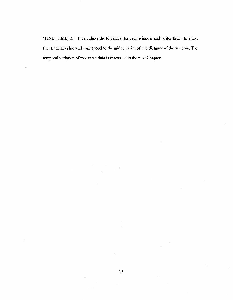
4.1 Averaged Temporal Voltage in dB versus Distance 67

4.1.1 Hallway 67


4.2 Large Scale Fading 70

4.2.1 Hallway 70


4.3 Spatial Variation of the Rician-K Factor 75

4.3.1 Hallway 76

4.3.2 Room H853-Microwave Lab 77

4.4. Conclusions 82

Chapter Five

Geometrical Optics Simulation 83

5.1 Modeling 83

5.1.1 Hallway 83


5.2 Voltage in dB versus Position 86

5.2.1 Comparing Measurements with Simulations 89

5.2.1.1 Hallway 89

5.2.1.2 Room H853- Microwave Lab 90

5.3 Path Loss Index "n " 92

5.3.1 Comparing Measurement and Simulated " n " Values 94

viii

5.3.1.1 Hallway 94

5.3.1.2 Room H853 -Microwave Lab 94

5.4 Large Scale fading 96

5.4.1 Hallway 96

5.4.2 Room H853 -Microwave Lab 98

5.5 Spatial Variation for the Rician-K Factor 100

5.5.1 Hallway 101


5.6 Comparison of Simulated and Measured KMLE 106

5.6.1 Hallway 107


5.7 Conclusions 112

Chapter Six

Conclusion and Future Work 114

6.1 Highlights 114

6.2 Contributions of the Work 116

6.2.1 Site Survey System 116

6.2.2 Time-Varying Measurements and Rician-K Factor 117

6.2.3 Space-Varying Measurements and Rician-K Factor 118

6.2.4 Simulations 118

6.2.5 Validation of the Methods for Evaluating the Rician-K Factor 119

6.2.6 The Three Methods For Evaluating The Rician-K Factor 120

IX

6.3 Recommendation for Future Work 121

References 122

Appendix A 129

Appendix B 139

Appendix C 145

Appendix D 146

Appendix E 147

x

List of Figures

Figure

2.1 Block diagram of the site survey measurement system. 21

2.2 The site survey system. 21

2.3 Block Diagram of the robot and the control unit. 23

2.4 Top view of the moving platform. 25

2.5 Bottom view of the moving platform. 25

2.6 Flow chart of programming the handy cricket board. 27

2.7 The transmitting unit showing the RF transmitter mounted on the moving

platform. 29

2.8 The inside of the RF transmitter. 29

2.9 The return loss of the antenna of the Tx unit. 30

2.10 The Rx unit showing the Rx antenna and the spectrum analyzer HP8569B. 31

2.11 The horizontal and vertical return loss of the Rx antenna. 32

2.12 Control unit and mobile platform communication (automation process). 35

2.13 Post processing programs flow chart. 36

3.1 General setup of the measurement system. 41

3.2 North-west corner map of the 15th floor of the EV showing the measurement

path along a hallway and the location of the receiving sleeve dipole antenna. 44

3.3 Concordia University EV15 hallway measurements setup part 1. 44

3.4 Concordia University EV15 hallway measurements setup part 2. 45

3.5 EV15 hallway time varying voltage(dB) ,Tx, Rx separation 60 cm. 45

3.6 EV15 hallway time varying voltage(dB),Tx, Rx Separation 294 cm. 46

xi

3.7 EV15 hallway time varying voltage(dB),Tx, Rx Separation 531cm. 46

3.8 EV15 hallway time varying power (dBm) ,Tx, Rx separation 1005cm. 47

3.9 EV15 hallway range of voltages versus distance. 47

3.10 Lower right corner map of Concordia University hall building 8l floor. The

microwave lab is room 853 and the location of the Rx antenna is denoted by a

dot, the path location of the moving platform is denoted by a straight line

facing it. 50

3.11 Concordia University H853 microwave lab measurement setup part 1. 50

3.12 Concordia University H853 Microwave Lab Measurement setup part 2. 51

3.13 H853 room time varying voltage (dB) ,Tx, Rx separation 30cm. 52

3.14 H853 room time varying voltage (dB),Tx, Rx separation 133.5cm. 53

3.15 H853 room time varying voltage (dB),Tx, Rx separation 238.5cm. 53

3.16 H853 room time varying power (dBm) ,Tx, Rx separation 450 cm. 54

3.17 Room H853 microwave range of voltages versus distance. 54

3.18 Time varying Rician-K factor values for the hallway. 64

3.19 Time varying Rician- K factor values for the microwave lab. 65

4.1 Time- averaged voltage versus distance for the hallway. 69

4.2 Time-averaged voltage versus distance for the microwave lab. 69

4.3 Comparison between the point-by-point measured voltage and the voltage

averaged over a 51.5 cm (4 X ) window for the hallway. 71


averaged over a 101.5 cm (8 A) window for the hallway. 71

xii


averaged over a l51.5cm(12A) window for the hallway. 72


averaged over a 51.5 cm ( 4 X ) window for the microwave lab. 74


averaged over a l 0 1 . 5 c m ( 8 / l ) window for the microwave lab. 74


averaged over a 151.5 cm (12/1) window for the microwave lab. 75

4.9 Space-varying K values for the hallway, sliding window size approx. 4 X . 79

4.10 Space-varying K values for the hallway, sliding window size approx. 8 X. 79

4.11 Space-varying K values for the hallway, sliding window size approx. 12 X. 80

4.12 Space-varying K values for the microwave lab, sliding window size

approximately 4 X . 80


approximately 8 X. — 81


approximately \2X. 81

5.1 GO 3D simulated version of the northwest corner of the 15th floor in

Concordia's EV building showing the Tx location and the path for the

received electric field. 84

5.2 GO_3D Simulated version of the microwave lab showing the Tx location and

the path for the received electric field. 85

xm

5.3 Simulated and calibrated measured results of voltage in (dB) versus distance

for the hallway. 91

5.4 Simulated and calibrated measured results of voltage in (dB) versus distance

for the microwave lab. 91

5.5 Simulated and measured results of voltage in (dB) versus distance for the

hallway showing path loss index n . 95

5.6 Simulated and measured results of voltage in (dB) versus distance for the

microwave lab showing path loss index n . 95

5.7 Large-scale fading (measured and simulated) scale for the hallway, window

size around 4/1. 97


size around 8/1. 97


size around MX. 98

5.10 Large-scale fading (measured and simulated) scale for room H853, window

size around 4/1. 99


size around 8/1. 99


size around 12/1. 100

5.13 Space-varying K for the hallway, window size around 4 X . 102

5.14 Space-varying K for the hallway, window size around 8 X. 102

5.15 Space-varying K for the hallway, window size around MX. 103

xiv

5.16 Space-varying K for room H853, window size around 4X . 105

5.17 Space-varying K for room H853, window size around 8/1. 105

5.18 Space-varying K for room H853, window size around 8 X. 106

5.19 Space-varying K comparison for the hallway, window size around 4X . 109

5.20 Space-varying K comparison for the hallway, window size around 8 X . 109

5.21 Space-varying K comparison for the hallway, window size around 12/1. 110

5.22 Space-varying K comparison for room H853, window size around 4 X . 110

5.23 Space-varying K comparison for room H853, window size around 8 X . 111

5.24 Space-varying K comparison for room H853,window size around 12 X 111

Al The LabVIEW Front Panel for A-AB VI. — 129

A2 The LabVIEW Block Diagram for A-AB VI. 129

A3 The LabVIEW Icon for A-AB VI. —129

A4 The LabVIEW Front Panel for AB_OR_D VI. 130

A5 The LabVIEW Block Diagram for AB OR_D VI. 130

A6 The LabVIEW Icon for AB_OR_D VI. 130

A7 The LabVIEW Front Panel for File VI. 131

A8 The LabVIEW Block Diagram for File VI. 131

A9 The LabVIEW Icon for File VI. 131

A10 The LabVIEW Front Panel for Scale Constants VI. 132

A l l The LabVIEW Block Diagram for Scale Constants VI. 132

A12 The LabVIEW Icon for Scale Constants VI. 132

A13 The LabVIEW Front Panel for GPIB VI. 133

A14 The LabVIEW Block Diagram for GPIB VI. 133

xv

A15 The LabVIEW Icon for GPIB VI. 133

A16 The LabVIEW Front Panel for Parsing VI. 134

A17 The LabVIEW Block Diagram for Parsing VI. 134

A18 The LabVIEW Icon for Parsing VI. 134

A19 The LabVIEW Front Panel for C-D VI. 135

A20 The LabVIEW Block Diagram for C-D VI. 135

A21 The LabVIEW icon for C-D VI. 135

A22 The LabVIEW Front Panel for Serial_com2E VI. 136

A23 The LabVIEW Block Diagram for Serial_com2E VI. 136

A24 The LabVIEW Icon for Serial_com2E VI. 136

A25 The LabVIEW Front Panel for controlmeasurments VI. 137

A26 The LabVIEW Icon for controlmeasurments VI. 137

A27 The LabVIEW Block Diagram for controlmeasurments VI. 138

xvi

Abbreviations

EMC

Tx

Rx

PDF

CDF

LOS

NLOS

GUI

EMI

LabVIEW

VI

GPIB

GO_3D

ISM

RF

PC

ASCII

KS test

PLL

VCO

Electromagnetic compatibility

Transmitter

Receiver

Probability Density Function

Cumulative Density Function

Line of Sight Path

None line-of-sight path

General User Interface

Electromagnetic Interference

Laboratory Virtual Instrumentation Engineering Workbench

Virtual Instrument

General Purpose Interface Board

Geometrical Optics Three Dimensional

Industrial Scientific Medical unlicensed band

Radio Frequency

Personal Computer

American Standard Code for Information Interchange

Kolmogorov-Smirnov Test

Phased-Locked Loop

Voltage controlled Oscillator

List of Symbols

K Rician value

K24 K found from second and fourth moment

Kn K found from first and second moment

KMLE K found from method of least square estimator

KCDF K found from the Cumulative distribution function

Kc K found using the Greenstein method

PL Path loss

Pt Transmitted power

Pr Received power

n Path loss exponent

Xa Zero-mean Gaussian random variable

v Receiver measured voltage.

Q Mean of the measured power

I0 ( ) Modified Bessel function of the first kind, zero order

/, ( ) Modified Bessel function of the first kind, first order

vm The voltage value (peak)

a2 Variance of the measured voltage

//, First moment of the measured voltage.

ju2 Second moment of the measured voltage.

ju4 Fourth moment of the measured voltage.

xviii

Chapter One

Background and Literature Survey

1.1 Applications and Motivations

For wireless communications and for electromagnetic compatibility, it is essential

to characterize electromagnetic fields within buildings. Electric field behavior is highly

dependent on the propagation environment [1]. Indoors, waves will experience reflection

and absorption by walls, floors, ceilings and people. The resultant field pattern is

unpredictable and complex [1]. Factors such as the materials of the walls, the frequency

and power will affect the resultant field pattern.

To characterize indoor wireless fields for a certain indoor geometry, the values of

the received field as a function both of distance and time must be known. These values

can be found by two methods: actual measurements or simulation programs. Actual

measurements are done by physically implementing a wireless channel (transmitter (Tx)

with known frequency and transmitted power and a receiver (Rx)), recording the received

field for variations in distance or time. This is called "site surveying". Simulation

programs are based on site-specific propagation models [2]. These models in turn are

based on detailed knowledge of the environment. Ray tracing, based on Geometrical

Optics, is one of these models and is used in this thesis as our simulation program -

specifically the GO_3D program [3][4].

1

The Rician probability distribution is often used in communications to model the

fading of the signal strength in a wireless channel in an indoor context. It is used to

evaluate that the probability that the signal strength is above the minimum needed for

good communication. In EMC it is used to determine if the signal strength is so strong

that it exceeds the immunity level of equipment. The immunity level of a device is

defined as the maximum value of electric field strength that an electronic device can be

exposed to without malfunctioning. A major objective of this thesis is to determine the

value of the Rician-K factor that characterizes a room or a corridor, both by measurement

and by simulation. For temporal variations of the signal strength, it will be shown that

typical Rician-K factor values are comparable to 60 dB. For spatial variation, typical

values are 10 to 20 dB.

The following Sections give a summary of radio propagation mechanisms and

parameters. Model classifications are explained, and an empirical model, specifically

"the Rician distribution" and its characterizing factor "Rician-K factor", are explained in

detail. Four methods from the literature for evaluating the Rician-K factor are

mentioned. Site specific models are also explained, including the thesis site specific

model of interest the "ray tracing method". An abbreviated summary of previous indoor

propagation measurements and measurement systems is presented, followed by the

detailed objectives of this thesis.

2

1.2 Basic Radio Propagation Mechanisms

Reflection, diffraction and scattering are the three basic propagation mechanisms

that govern radio propagation [1]. Reflection occurs when an electromagnetic wave hits

an object that has large dimensions compared to the wavelength of the wave. The

reflection coefficient is the parameter that relates the incident wave to the reflected wave.

This coefficient is a function of the material properties and construction of the surface

that the wave reflects from. It also depends on the wave polarization, the angle of

incidence and the frequency of the propagating wave [5].

Diffraction occurs when the radio path between the transmitter and the receiver is

obstructed by a surface that has a sharp edge [6][7]. Diffraction is based on the concept of

Huygens' principle [5], which states that all points on the waveform are sub sources for

the production of secondary wavelets and that these wavelets combine to produce a new

wavefront. Other references [8] explain Huygens' principle as a method for finding

subsequent positions of an advancing wavefront.

Scattering occurs when an object in the radio path has dimensions much smaller

than the wavelength. Scattering can be described as disorganized reflection from a rough

surface. Scattering sometimes adds extra strength to the received signal in a mobile

environment. Objects such as lampposts and trees tend to scatter energy in all directions

[5][8]. Scattering can make the actual received signal stronger than was predicted by

reflection and diffraction alone. It occurs when the reflected signal impinges upon a

3

rough surface; the reflected energy is spread out (diffused) in all directions due to

scattering [5]. A scattered signal is a multipath signal since the signal traveling from the

Tx to the Rx will undergo multiple paths [9].

The resulting field obtained from the use of the propagation models is often very

complex. It is a common practice to make a simplified model for a particular application.

The next Section will discuss some of the more popular models and their associated

parameters.

1.2.1 Radio Propagation Parameters

Path loss (PL) is one of the important parameters needed for the analysis of indoor

radio-wave propagation. It is a measure of the losses the signal suffers when it reaches

the receiver [6][7][10][11]. It is given as

PL(dB) = 10 log^- (1.1) r

where P, is the power transmitted from the transmitting antenna and Pr is the power

received at the receiving antenna. This measured parameter will help to determine the

models used for the mobile channel. Some other studies [5][6][11] express path loss as a

function of distance (<i) and with the following formula

4

PL(d) = PL(d0)+lOn\og(d/d0)+Xa (1.2)

where n is called the path loss exponent [5] n is equal to 2 for free space. The value of

n is less than 2 for indoor wireless channels. For indoor wireless channels this value

depends on the frequency being transmitted, the geometrical shape of the environment

being measured, the materials used in the indoor environments and the antenna

height[12].XCT is a zero mean Gaussian random variable which accounts for the

variation in average received power that happens when this type of model is used.

1.3 Model Classification

All models used in the indoor propagation channel are either empirical models or

site-specific models. The main difference is that empirical models are easier to

implement, whereas site specific models are more accurate but require a large amount of

input data and considerable computation [7]. These models could be used on two types of

data format for the received signal strength. "Large scale propagation" characterizes the

received signal strength over large distances. It is also called "large scale fading". "Small

scale propagation" accounts for the rapid fluctuation of the received signal over short

distances. It is also called "small scale fading" or "Rayleigh fading" because if the

multiple reflective paths are large in number and there is no LOS component the received

signal is described by the Rayleigh probability distribution [5]. To show the "large scale

fading" behavior of a signal with "small scale fading" behavior, the "small scale fading"

will be averaged using a sliding window. The sliding window starts with the first

5

distance point and combines the number of points required to change the scale of the

measured data from small to large distances. The next window starts by dropping one

point on the left and adding one on the right, keeping the same window size, and so on.

The next step is to average the data values for each window. The average value

corresponds to the middle of the size of the sliding window. The next Section will speak

about the Rician distribution as an empirical model example for a wireless channel, the

empirical model used in this thesis.

1.3.1 The Rician Distribution "Empirical Model" and the Rician-K Factor

One of the important parameters that must be known for the wireless channels

that follow the Rice distribution is the Rician-K factor. The Rician-K factor is a

parameter that characterizes the Rician probability distribution and which is also called

the Rice distribution. A wireless channel can be statistically characterized to follow a

Rician distribution when there is a dominant signal present such as the (LOS)

propagation path between the transmitter and the receiver. Some studies

[14] suggest that for extensive temporal variations or fast fading analysis when there was

no LOS between the Tx and the Rx, the distribution of the measured data was also Rician

and it fits the measured data inside office and university buildings. The Rician

distribution probability density function (PDF) is given by [1][17].

w Q n J ° v n (1.4)

6

where v is the measured voltage at the receiver of the wireless link, K is the Rician-K

factor which is given by v^/2cr2, vm is the voltage value (peak) of the LOS path

between the Tx and the Rx of the channel, cr2 is the variance of the measured voltage of

the receiver of the wireless link, CI is the mean of the measured power of the receiver at

the wireless link, and I0 ( ) is the modified Bessel function of the first kind and zero

order.

The cumulative distribution function (CDF) of the Rice distribution is given by[18]

F(V) = 1 - exp K + -2a2

'aJlX^ (v42X^

V v J \

(1.5) J

where Im( ) is the modified Bessel function of the first kind and m order

The Rician probability distribution is used to model wireless channels where

there is a strong deterministic signal component and a lower-level random signal

component. In this thesis, the strong signal component is associated with a line-of-sight

(LOS) path joining the transmitter to the observer. The random signal component models

the many reflections from the walls, floor and ceiling. The phase of the field associated

with each reflection path is modeled as uniformly distributed, and the various reflected

fields combine to form a random variable with a Rayleigh distribution. The Rician K

factor is the ratio of the power in the direct field to the power in the reflected field. When

the direct field strength is much larger than the reflected field strength, K is large, such

as 60 dB, and the Rician distribution can be approximated as a Gaussian distribution with

a small spread of values around the mean, corresponding to a low standard deviation [7].

The field strength deviates very little from the mean value and is almost deterministic.

When the direct field strength is not very much greater than the reflected field strength,

K is not large, such as 10 dB, and the Rician probability density shows a large spread of

values around the mean, corresponding to a large standard deviation, and the Rician

distribution can be approximated with a Rayleigh distribution [7]. The field strength has a

large random component and varies over a wide range.

1.3.2 Rician K Factor Evaluation

Given a set of measured voltage data in linear scale {v, : / = 1: N } where N is

the number of samples being measured, and this set, which is the square root of the set

of power measured data in linear scale {p, : / = 1: N}, then from the set of measured

voltage data, the Rician-K factor can be estimated. Four methods to estimate the Rician-

K factor are found in the literature. In [19], the Rician-K factor found from this method

will be called here KG in honor of first author Greenstein. In [20][21] the Rician-K factor

is found from two methods. One is called here/C24 because it is based on finding the

second and fourth moment. The other method is called here Ku because it is based on

finding the first and second moment. In [20] [22] the Rician-K factor found from this

method is called here KMLE because it is based on the method of least square estimator.

Each method will be described in detail in Chapter 3.

8

1.3.3 Ray Tracing "Site Specific Model"

One of the site specific models used in radio propagation is the ray tracing

method, based on geometrical optics. It assumes that energy from the EM wave can be

considered in terms of rays. This is a simple representation of the EM wave mechanisms

[2]. One type of ray tracing is the image method. It assumes that when the ray is reflected

from a wall, an image of the source is generated behind that wall, which gives back the

reflected wave with an attenuation factor. This concept is the basis of the GO_3D

program used in this thesis [3][7][9]. In this thesis the G 0 3 D Ray Tracing program will

be used [3][4]. The GO_3D Ray Tracing program shows the field behavior when

radiating from the transmitter source; at each wall rays are incident on, and then each

image source acts as another transmitter and transmits the ray again. This is equivalent to

a ray that is incident on the wall and then reflected from the wall again, the number of

reflections to be considered on each wall gives the number of levels on the image tree.

More details about the image tree concept can be found in [3].The next Section will speak

about previous studies on indoor propagation measurement systems.

1.4 Indoor Propagation Measurement Systems

When any measurement campaign is performed, the need for a measurement

system arises. In all measurement campaigns, although the measurement systems differ

from each other, they all have common parts. Each system consists of a transmitting

unit with known parameters such as the gain of the transmitting antenna, transmitting

9

frequency, output power, polarization, and radiation pattern. The receiving antenna, also

with known antenna parameters and the added value of the antenna factor to transform

the voltage measured to an electric field, and measuring devices such as a spectrum

analyzer for CW wave single tone frequency or a vector network analyzer for broad

band frequencies connected to a computer, and the receiver antenna moving on a

predefined path with known steps and via different tools all combine to make up the

measurement system. This Section describes measurement systems found in the literature

for indoor propagation.

In [23] an automated guided vehicle (AGV) was developed to use in indoor

propagation measurements. This AGV provides an accurate estimate of position, which

is very useful in measurements. Many types of AGV's rely on what is called dead

reckoning, where distances are computed by integrating the distance traveled by one or

more vehicle wheel. Here the AGV carries the microwave receiver, including the

receiving antenna and spectrum analyzer used in measurements. It has a front wheel

containing a steering motor and a drive motor. Each rear wheel has an optical shaft

encoder that is translated into distance and path curvature information .

In [24], the AGV is called a robot. The concept has it following a predefined path

on the ground. Two sensors on the front of the robot follow a predefined path, made with

black electrical tape on the floor. The receiver was mounted on the top of the robot using

a PVC pipe, holding a calibrated dipole antenna connected to a spectrum analyzer. The

robot platform had one fixed front wheel with an optical encoder to determine the

10

distance moved by the robot, and two rear wheels. The transmitter in the system was an

analog cellular telephone with 850 MHz frequency and 600 mW output power or an RF

signal generator at 1900 MHz.

In [25] the measurement approach was quite different. The measurement was to

detect electromagnetic interference (EMI) in a hospital environment and at fixed

locations. The approach has more to do a with a computer system, which had a general

user interface (GUI) to take readings in various hospital environments, and to show if any

cases of EMI occurred in the hospital environment. The computer program used in

measurements uses Lab VIEW programming language. It is the state-of-the-art program

in measurements, and it enables the computer to take readings from a spectrum analyzer

connected to the computer via a GPIB card. Lab VIEW is a visual programming

language provided by National Instruments company and it is a very useful tool in data

acquisition. LabVIEW version 8.0 has been used in this thesis [26][27].

In [28] a mobile robot platform was developed to provide a mechanism to

determine the accurate position of the robot using odometry equations. These are easy to

implement but there is the drawback of error accumulation as the travel distance

increases. The general concept of the robot mechanism is the same as in [24] but with

different design layouts and different microcontrollers. The next Section provides

information about indoor propagation measurement results.

11

1.5 Indoor Propagation Measurement Results

In any measurement campaign, after the data has been collected a meaningful

interpretation must be given. This meaningful interpretation is done by statistical

interpretation. One method to interpret the data is to characterize it using certain

statistical parameters. This Section gives a survey of the characterization of measured

data from measurement campaigns using the Rician-K factor.

In [29] measurements were performed to investigate the Rician K Factor (in dB)

for four different measurement environments, and for LOS and NLOS cases. The four

different measurement environments were: small room, hallway, stairwell and a lecture

theatre. The small room had work benches heavily equipped with computer equipment.

The hallway was free of any obstructions and had doors both sides closed during the

measurements The hallway was open at one end. The stairwell had two set of stairs

going downwards and one doorway. The lecture theater was a typical lecture theater

environment. For all environments the Tx antenna was moved to eight locations and the

Rx antenna was at a fixed location. For the small room the K value was the highest for a

LOS case and the lowest for the NLOS case, for the hallway the K value was

approximately the same for all positions. For the stairs, the lowest value was in a

location that had an obstructed line of sight, and the highest one was for the location that

had a clear LOS . In the lecture theatre all values of K were virtually the same. The

values of Rician-K factor obtained ranged from 1.8-4.7 dB.

12

Another indoor measurement study in a hospital environment [25] used

completely automated software in analyzing and taking measurements. The software was

produced using Lab VIEW. The software, known as PRISM, was designed for ease of

use and can be monitored from remote areas. Measurements were done for the electric

field at the same points for different times in the 2.4 GHz ISM frequency band. Results

showed some constant behavior for the electric field during the different times of

measurements.

Another study [30] was done in Spain at the University of Cantabria campus.

Three measurement scenarios were performed. Each scenario corresponds to a different

environment. The measurement system was totally automated. The receiver was moving

and the transmitter was fixed. The movement of the receiver was controlled by the

computer via a serial port, and at the same time the computer recorded the readings from

the spectrum analyzer using the GPIB interface. LOS path scenario measurements for 1.8

and 2.5 GHz were made. The same scenarios were also simulated using a GO computer-

based program. For the results of measurements and simulations the values of the Rician-

K factor that were calculated showed a good agreement. The Rician-K factor was found

for the entire path, denoted as Kwhole, and for windows along the path which were

represented by their maximum, minimum, and mean value denoted by Kmax, Kmin, and

Kmean. The values of Rician-K factor found ranged from 0-3.45.

13

In [31] measurements were performed at 2.4 GHz, in a large engineering lab at

the University of Oxford. The Rician- K factor was investigated, and it showed that it

has constant and small values for NLOS conditions along the path being measured. For

the LOS conditions, the Rician-K factor goes up to 170, for a corresponding Tx, Rx

separation of 2 meters, and then is varies After the 2 meter Tx, Rx distance the Rician-K

factor value varies, down to a minimum value of approximately 10 at a distance of 30

meters. Also, the value of K for LOS conditions shows a decreasing behavior as the Tx,

Rx distance increases. The values of the Rician-K factor found ranged from 0-200.

The Rician-K factor values were evaluated from a large set of wireless indoor

propagation measurements in [32]. The data collection procedure was organized in the

following manner: both the transmitting and the receiving antennas were mounted on an

arm that rotated in the horizontal plane. Narrowband RF power was measured at 1.92

GHz and recorded. One thousand data points were calculated as both the Tx and the Rx

were moving. This procedures was repeated at 400 locations. Some locations were line of

sight and others were obstructed locations. The author calculates the Rician-K factor

based on finding the mean and variance from the 1000 data samples calculated at each

location. The author does not state the reference he relied on for the method used to

calculate the Rician-K factor. His calculated Rician-K factors for the measurements he

performed showed peaks and nulls, the values ranged from 20 to -25 dB. The Rician-K

factor plotted graph shows that the high values were for line of sight locations, while the

low values were for obstructed locations.

14

In [33], measurements were performed at 2.4 GHz, at the cooperative research

center for broadband telecommunications and networking laboratory at Curtin University

of Technology, Australia. They used a typical laboratory environment, with a middle

work bench, two right and left side benches and a door open to the hallway. The

measurement scenarios had the Rx antenna fixed and ten different locations for the Tx

antenna were considered. One was an LOS condition facing the open door at the hallway,

and the remaining nine others were NLOS conditions. At each of the ten Tx, Rx, fixed

wireless link there were three scenarios when measuring the received power, no

movement, three people moving, and six people moving in a similar manner within a two

meter radius around the Rx. Four representative Rician-K factor value results are shown

from the previous arrangement made for measurements. Three values of K from the

four shown were for the three people moving around the Rx antenna. The highest value

of K was obtained for the largest NLOS Tx, Rx separation. The fourth value was for six

people moving around the antenna, which gave a the smallest value of the Rician K

factor for the whole four which is 1.3. The four values for the Rician K factor shown

were 1.3, 2.0,2.0 and 8.7.This shows the Rician-K factor is higher when less people are

moving around the measurement setup and higher at larger Rx, Tx separation for NLOS

conditions.

Rician-K factor measurements were performed in a multi-storied building in [16].

These survey results were used to find the Rician-K factor for a spatial variation of the

received power. Here it was determined that higher values of K are found in LOS

conditions while low values of K are found in NLOS conditions, and typical values for

15

the Rician-K factor were from 0 - 6.6. In [34], the Rician-K factor for the temporal

variations of the RF received power was found. Estimating the Rician-K factor value was

based on the best fit of the measured data empirical CDF with the CDF found from

applying the Rician CDF formula. The highest value of K was for a short LOS path and

the lowest value of K was for a location of the Tx where the multipath signals dominated

the main path. The measured Rician-K factor ranged between 0-20. In [35],

measurements were done in a tunnel with different scenarios. The results show that slow

fading did not match the lognormal distribution as sometimes anticipated by other

references. Also shown was that the fast fading of measurements in straight Sections in a

tunnel correlates well with the Rician distribution while fast fading signals for curved

Sections does not closely fit the Rayleigh distribution, and higher frequency signals

exhibit more fluctuations for the received signal versus distance. The comparison criteria

was developed by comparing the CDF for the measured data with a theoretical Rician or

Rayleigh CDF. The next Section presents the objective sets for this thesis.

16

1.6 Objectives

The objective of this thesis is to study the behavior of the Rician-K factor for an

indoor wireless channel. Four methods from the literature are used to calculate the

Rician-K factor from the measured received power. Two environments are used as case

studies: a hallway and a lab. Measurements are performed using a site survey system

designed to be an automated system and that accounts for spatial and temporal variation

of the received signal power. Simulations for the same environments are done using a

ray tracing program, in order to have a simulated version of the measured data that

accounts for spatial variation only. The simulated data version is compared with the

measured data to see if the ray tracing models generated for the two environments

provide a good match with measured data. The comparison between measured and

simulated data is based on comparing the following: small scale fading, path loss

index n, the space varying Rician-K factor and the large scale fading for both measured

and simulated data.

17

1.7 Overview of Thesis

Chapter 2 describes the site survey measurement system. For the hardware,

survey supporting block diagrams and pictures are given with full explanation of each

part. For the software, flowcharts are given for the programs used to operate the robot

and for the control unit. The flow chart of the control unit program also shows the

communication between the control unit and the robot's microcontroller.

Chapter 3 investigates the temporal variation of the received power. Measured

data was obtained for two environments, the hallway and the microwave lab. Four

representative distance points between the transmitter and the receiver were chosen, and

the time varying received voltage level is graphed. The difference on a linear scale

between the maximum and the minimum values for time varying voltages at each

distance point are graphed in dB and are called as the range of variation of voltages. Four

methods for calculating the Rician-K factor from measured sampled data from the

literature are presented, and the time varying Rician-K factor values are calculated

using all four methods.

Chapter 4 investigates the spatial variation of the Rician-K factor for two

environments, the hallway and the microwave lab. At each receiver, transmitter

separation of the average value of the time varying received voltage is found. The

average value is graphed as a function of the distance between the transmitter and the

receiver. This is also known as the small scale fading of the measured data. A sliding

18

window is moved along the small scale fading measured data. The large scale fading for

the measured data is found by averaging each sliding window set of data and

corresponding this value to the middle point of the size of the window. Then the space

varying Rician-K Factor values are calculated for each set of data of the sliding

window, using the methods presented in Chapter 3.

Chapter 5 shows how ray-tracing method is used to simulate two environments,

the hallway and the microwave lab. The ray-tracing based GO_3D program calculates

the received electrical field. A method to calculate the received voltage across a 50 ohm

load from electric field strength is presented, comparison between measured and

simulated voltages is based on four factors, small-scale fading, path loss index, large

scale fading and space-varying Rician-K factor.

Chapter 6 summarizes the thesis and presents the conclusions. The best method

to calculate the Rician-K factor is described, based on comparison between measured

and simulated data, and the agreement and disagreement they present based on the

comparison criteria used. Some recommendations for future work are presented.

19

Chapter 2

The Measurement System

2.1 Introduction

In this Chapter the complete site survey system will be described, including the

hardware utilized and the software programs that were developed.

2.2 The Site Survey System

Figure 2.1 shows a block diagram of the site survey system, which has three main

parts: the transmitting unit; the robot; the receiving unit and the control unit. The

transmitting unit transmits between 2.3 to 2.5 GHz in the ISM band. The robot is a

microcontroller-based moving platform that is equipped with a 900 MHz wireless link to

communicate with the control unit. The receiving unit consists of a calibrated dipole

antenna connected to the HP8569B spectrum analyzer, and the control unit is composed

of a desktop PC equipped with a GPIB card and a 900 MHz wireless communication link

to the robot. Figure 2.2 shows the actual site survey system used in measurements, the

robot carries the transmitting unit and moves following the white tape on the floor.

20

Rx Unit V

Rx Dipole

HP8569B Spectrum Analyzer

Control Unit

900 MHz Wireless link

GPIB

PC

Serial port

V

Vr 900 MHz Wireless link

Robot

Figure 2.1 Block diagram of the site survey measurement system.

Figure 2.2 The site survey system.

21

The site survey measurement system was designed to measure the spatial and

temporal variations of the received RF signal power level, and then write them to a text

file on the computer in a predefined format. This text file will work as an input file for

post processing applications. This site survey measurement system has already gone

through two versions[12][36]. The first was only a prototype of a moving platform with

the Tx unit [36], and the second version, semi-automated, has a moving platform as

described here [12]. The control unit (PC) has a Lab VIEW program that captures data

from the spectrum analyzer using a GPIB card for communication. Control of the robot's

movement is done using a 900 MHz wireless link between the control unit and the robot.

The current version of the site survey system is fully-automated using a Lab VIEW

program. This program has a control part and a measurement part work with each other

in a correlated manner to provide this automation property.

The automated concept of this system which is the communication between the

robot and the control unit is explained in Section 2.6 of this Chapter. Each part of the site

survey system will be described in detail in the following Sections. The earlier steps

taken to make the prototype of the mobile platform and some measurements related to it

can be found in [12][36].

22

Encode Left

WUinkQGOMHz

, i .

Pcower Supply 9 VolJ

Interfax &es$rd

Sensor port a

- • } Handy Ct3ck«4 Main Board

Power Supply 1.5 VoMAABaawfes

h Optical

Right wtw)«l

Wheel

Motor ForE D 1 A output

Narsdiy Crieket Expansion Board

Motor Port C 1 Ao^fKJt

Sensor port

12VCR Battery , 1.3Amp$£

Ur* Tracking Sensor

Fixed Front Wtlfifil

Right Rear Wheel

Desktop PG

[ Serial Port

« '-.

-*

WretessUnk 300 MHz

M<

J Coram!

CwilrBt

P W W

Figure 2.3 Block diagram of the robot and the control unit.

23

2.3 The Robot

Figure 2.3 is a block diagram of the robot and the control unit, and Figures 2.4

and 2.5 show photographs of the robot from the top and the bottom, respectively. The

"Handy Cricket Board" controls the operation of the robot [12][36], shown as a block

diagram in Figure 2.3, and close to the right rear wheel of the robot in Figures 2.4 and

2.5. It has two sensor ports, connected to the optical encoders that are coupled to the rear

wheels, and which are operated by two DC motors. These two DC motors are shown as

block diagrams in Figure 2.3 and are facing the two rear wheels in Figures 2.4 and 2.5.

The two DC Motors need to draw a high current to operate, and this high current is

provided to them via the Handy Cricket extension board, shown as a block diagram in

Figure 2.3 and located near the front wheel in Figures 2.4 and 2.5. This board is powered

by a 12 volt battery with 1.3 ampere, as shown as a block diagram in Figure 2.3 and

located between the two rear wheels in Figures 2.4 and 2.5. The Handy Cricket extension

board has two motor ports and four sensor ports: two of these sensor ports are connected

to the line tracking sensor board, shown as a block diagram in Figure 2.3 and mounted on

two supporting metal stands behind the front wheel, as can be seen in Figures 2.4 and

2.5. The line tracking sensor board facilitates the movement of the platform on a

predefined path, which is a masked tape that is applied to the floor where the robot will

be moving. The tape must be black if the floor is light-colored and white if the floor is

black or dark- colored. More details can be found in [12].

24

Figure 2.4 Top view of the robot.

»m?m S**a*5

-..-jAsi-- '•'•• « V j ; i W

•MB

W * *

Figure 2.5 Bottom view of the robot.

25

2.3.1 The Cricket Logo Software

The robot is controlled by the Handy Cricket board, which uses a programming

language called "Cricket logo". This cricket board includes a "Cricket logo" interpreter.

Programs in "logo" are downloaded from a PC to the cricket board via the infra-red (IR)

cricket serial interface and then executed independently on the microcomputer cricket

board. In other words, once the "logo" program is downloaded to the robot's computer, it

can be executed on the Cricket board.

2.3.2 Programming the Handy Cricket Board

The flow chart for the "logo" program used for the robot's microcontroller is

shown in Figure 2.6. When the robot is powered up, the microcontroller is in 'wait'

mode. The microcontroller waits for an ASCII character to be received via the serial

port from the PC that controls the measurement system. When an ASCII character "A"

is received, this signals the start of the measurement campaign, and in reply the

microcontroller sends an ASCII character "AB" to the control unit. When an ASCII

character "C" is received, the robot follows the tape on the ground for a distance of 1.5

cm and then stops. Then an ASCII character "D" is sent to the control PC. If an ASCII

character "E" is received by the microcontroller, this signals the end of the measurement

campaign. Further details can be found in [12J[36] and a listing of the "Cricket logo"

program is in Appendix B.

26

Start

Wait until an ASCII character is received.

No

Has an "E" been received

yes

Sends the ASCII characters "AB"

yes

Robot starts moving following the tape on

ground, stops after 1.5 cm.

Sends an ASCII character "D"

yes

End

Figure 2.6 Flow chart of programming the Handy Cricket board.

27

2.4 The RF Transmitting Unit

The RF transmitting unit of the site survey system is a battery-operated CW

transmitter. It is mounted on the robot, which moves it along the path of the tape on the

floor in the microwave lab or hallway. Figure 2.7 shows the RF transmitting unit

mounted on the robot moving platform. The theory behind how the RF Transmitter works

is based on the concept of Phased-Locked Loop (PLL) [11][36][37]. Figure 2.8 shows

the circuit of the RF transmitter, the board on the right is the PLL circuit. It contains a

voltage-controlled oscillator (VCO) and a loop filter (LF). This board has one input, a

crystal oscillator (XO) on the lower left part of the board, used to stabilize the

frequency for the transmitting unit. The output of the PLL circuit is on the upper left part

of the board and is used as an input to an amplifying board, which amplifies the input

frequency power level from 0 dBm to 10 dBm. The frequency range of the RF transmitter

is the ISM band from 2.4 to 2.5 GHz.

28

Figure 2.7 The transmitting unit showing the RF Transmitter mounted on the robot.

^ ^ K ^ « - ^ ' ' '

Figure 2.8 The inside of the RF transmitter.

29

The antenna mounted on the Tx unit is a monopole. The length of the monopole

was trimmed to have a return loss at the input port better than -lOdBm for the

frequency range from 2.4 to 2.5 GHz, as shown in Figure 2.9. The return loss was

measured using an HP8720 Network Analyzer.

T x R n t e n n o R e t u r n L o s s

r e q u e n c y

Figure 2.9 The return loss at the input port of the antenna of the Tx Unit.

2.5 The Receiving Unit

The receiving unit shown in Figure 2.10 consists of a calibrated sleeve dipole

provided by ETS, LINDGREN Model #3126. It is connected to an HP8569B spectrum

analyzer. The spectrum analyzer is used to measure the RF power received by the sleeve

30

dipole working into a 50 ohm load. With the robot and the transmitter at a fixed location,

the power received by the spectrum analyzer is measured at 30 two-second time

intervals, in order to measure the temporal variation of the signal. To measure the spatial

variation, the robot follows a path along the floor defined by applying a masking tape to

the floor. At each position on the path, 30 time samples of the received power are taken

and written to the output data file.

Figure 2.10 The Rx unit showing the Rx Antenna Model # 3126 and the HP8569B

spectrum analyzer.

31

2.5.1 The Rx Antenna

The Rx Antenna is a calibrated sleeve dipole. It is an omni-directional antenna in

a plane perpendicular to the dipole axis. The antenna design allows it to be end fed to

avoid feed point and cable interactions that affect the radiation pattern. This antenna

covers the frequency range from 2.3 to 2.6 GHz. The antenna is mounted on a tripod

during measurements. The return loss for the Rx sleeve dipole antenna for both a

vertical and a horizontal orientation are shown in Figure 2.11. This was measured using

the HP8720 network analyzer. The return loss is somewhat different for the two

orientations because the measurements were taken on a lab bench, rather than in an

anechoic room. The antenna interacts with the nearby objects.

-* * Hor izonto l ReturnLoss ~© o U e r t i c o l R e t u r n L o s s

£ 4 5 0 E50E

Frequency I MHz 2 5 5 0

Figure 2.11 Horizontal and vertical return loss of the Rx antenna.

32

2.6 The Control Unit

The control unit consists of a desktop PC equipped with a GPIB card and a 900-

MHz wireless link connected to the serial port of the PC. The GPIB card connects the PC

to the HP8569B spectrum analyzer of the Rx Unit and is used to capture data from the

spectrum analyzer. The 900-MHz wireless link is used to communicate between the

Mobile platform and the Control Unit using ASCII characters. The program used to

control the robot movement and take spatial and temporal RF received power level

measurements is written in Lab VIEW. The programming flow chart is shown in Figure

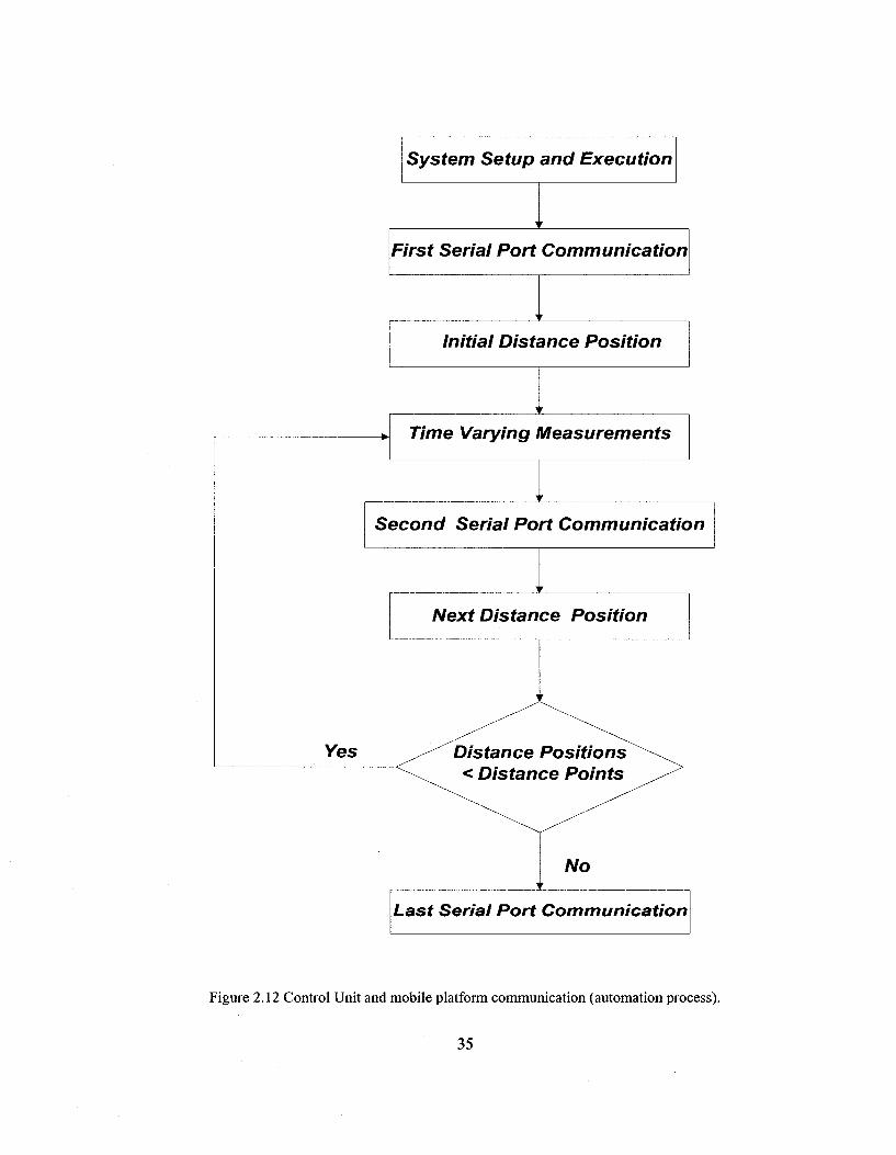
2.12, and the description of each block diagram of the flowchart is given below.

1. System Setup and Execution: the robot is powered on, the controlling program

in the Handy Cricket board is started, and then the Lab VIEW program is started after all

its input parameters are defined.

2. First Serial Port Communication: the LabVIEW program is started on the

controlling PC, and starts serial port communication between the controlling PC and the

robot's cricket board. The PC sends an ASCII character "A" and the robot responds with

"AB".

3. Initial Distance Position: the initial distance is checked and the initial position is

written to the text file on the controlling PC.

33

4. Time Varying Measurements: the Lab VIEW program reads the spectrum analyzer

30 times, at a time interval of 2 seconds between readings. The received power is

determined at the operating frequency and then the time and received power are written

to the output text file.

5. Second Serial Port Communication: the Lab VIEW program sends the ASCII

character "C" to the robot. The robot responds by moving an increment of 1.5 cm. This

distance is determined by the optical encoders attached to the wheels of the robot. Next,

the platform sends the ASCII character "D" to the control unit to acknowledge moving

and stopping.

6. Next Distance Position: the new position is written in the text file on a new line.

The next distance position value is the previous position value plus the distance

increment. The spectrum analyzer reads the received RF power at 30 time intervals and

writes them to a text file. If there are more positions for measurements, the program goes

to step 5.

7. Last Serial Port Communication: when all distance points have been reached and

the corresponding RF power time-varying measurements have been recorded, the

Control Unit sends the ASCII character "E" to the moving platform to terminate the

measurements and the Lab VIEW program shows the operator a message that indicates

measurements have finished.

34

System Setup and Execution

First Serial Port Communication

Initial Distance Position

Time Varying Measurements

Second Serial Port Communication

Yes

Figure 2.12 Control Unit and mobile platform communication (automation process).

35

Control and Measurment Program

lnput.txt

MAKE TIME FILES

• • •

Range.txt ) (Distance.txt) (Time1.txt) (Time2.txt

FIND TIME K

ktime.txt

1 MAKE WINDOWED DATA

Slowfade.txt) (window1.txt) (Window2.txt

FIND SPACE K

Kspace.txt

Figure 2.13 Post-processing programs flow chart.

36

2.7 Post Processing of the Measured Data

The results of the measurements must be analyzed in order to give an

interpretation of the measurements campaign. The Lab VIEW program report will be

named as input.txt to start analyzing its data. In this thesis the Rician-K factor values for

the spatial and temporal variation of the received signal power will be calculated from the

measured data, according to the methods mentioned in Chapter one. A sample of the

text file "input.txt" generated is shown in Appendix C.

Figure 2.13 shows a flow chart of the post processing programs process. It starts

with the measurement and control program of the control unit. The output of this

program is the "input.txt" which contains the results of the measurement campaign. This

text file contains the time varying received power for each Rx, Tx separation.

The "input.txt" file is used as an input for the "MAKETIMEFILES" program.

This program sorts each Rx, Tx distance reading and puts them in an individual file;

each file is called Timel.txt,Time2.txt, ..., till Time(n).txt, where n is the number of

distance points being measured. These file formats have a header that shows the distance

value for each file, and which indicates that the two-column data format displays distance

on the left and the corresponding linear voltage on the right. This program generates a

text file called "Distance.txt" with two-column data, the first column on the left displays

the distance value and second column on the right is the corresponding average time-

varying received voltage. The program also generates a file called "Range.txt" which is

37

similar to the "Distance.txt" file except that the second column is the maximum divided

by minimum of each time(n).txt file instead of average. Since all results are in linear

scale and will be plotted later in (dB) format the range file is the division of maximum by

minimum which is the equivalent of difference between the maximum and minimum

value in (dB).

The next program is "FINDTIMEK". This program will read each Timel.txt,

Time2.txt,...Time(n).txt and calculate the K value using five methods: Kc,K24,Kn,

KCDF, and KMLE, mentioned in Chapter One. This program uses the "halving interval"

method to find the root of the equations of Kn and KMLE.

The program "MAKEWTNDOWEDDATA" arranges the "Distance.txt" in

another format using a sliding window with a predefined number of measurement

points or samples. This sliding window moves along the data starting from the first data

point. The next sliding window starts with the second data point and discards the first

data point on the left and so on until all of the path is completed. This program generates

text files called windowsl.txt,windows2.txt, windows(n).txt, and generates a file

called "large_scale.txt". The file "large_scale.txt" has two-column data. The column on

the left is for the middle of the distance corresponding to each window, and the average

of the voltage for each window is displayed on the right.

The program "FINDSPACEK" calculates the K value using four methods

mentioned in Chapter one, Kc,K24,Kn, and KMLE that are also used in

38

"FIND_TIME_K". It calculates the K values for each window and writes them to a text

file. Each K value will correspond to the middle point of the distance of the window. The

temporal variation of measured data is discussed in the next Chapter.

39

Chapter 3

Temporal Variation

3.1 Introduction

In this Chapter, temporal variations of the received electric field for two

environments are considered: the hallway and the microwave lab. For each environment

the time variations of the received signal in volts (dB) for four fixed receiver (Rx),

transmitter (Tx) distances are shown. The four methods used to evaluate the Rician-K

factor mentioned in Chapter one are explained in detail. Time-varying Rician-K factors

for both environments are plotted and explained. This Chapter shows that the time-

varying signal is constant, and that the possible movement of people near the Tx and

the Rx caused small variations in the time-varying received signal. The time-varying

Rician-K factor found using the four methods from the literature presented a good match;

KG IK24 are the same and are the best methods to be considered when evaluating the

time-varying Rician-K factor in a wireless channel.

40

3.2 Voltage in dB versus Time

Field strength may vary over time at a fixed distance from the source. Therefore

it can be important to understand the behavior of the electric field as a function of both

time and distance. In the following Sections, representative distance points between the

transmitter and the receiver are chosen to show the behavior of the time-varying

received voltage for the two environments, the hallway and the microwave lab. The

setup of the measurement system is shown in Figure 3.1. The robot moves in steps of

1.5 cm. At each step-distance, 30 time-varying readings of the received voltage were

taken, at a time interval of two seconds. The readings obtained from the spectrum

analyzer are in power (dBm) and the plotted graphs are in voltage (dB).

Rx

Tx

IF f%x H4&S9M

Robot

IF Tx

Height

( 5 > € ) A

fxr OSstance

r -Ssj

Figure 3.1 General setup of the measurement system.

41

3.3 Conversion from dBm to Voltage

The spectrum analyzer measures the power delivered to a 50 ohm load, in dBm.

This Section describes how to find the voltage across the 50 ohm load, starting with this

equation

^ = 1 0 1 o g f P X

lmW (3.1)

where PdBm is the power measured from the spectrum analyzer in dBm and P is the

power measured in linear scale. The power reference level is 1 milliwatt. By replacing the

linear scale of power with the equivalent voltage, (3.1) can be expressed as

20 log VO.OOLR

(3.2)

where v is the measured voltage in linear scale and R is the resistance. Arranging (3.2)

to express the linear voltage in terms of the measured power in dBm and replacing R

with a 50 ohm matched load, we obtain

v = >/0.001-5o[lOW20]. (3.3)

42

This equation is used to transform the measured power in dBm from the spectrum

analyzer to voltage in linear scale. All results obtained are in linear scale and will be

plotted using dB scale. The reference level for voltage in dB is 1 volt RMS.

3.3.1 Hallway

The hallway of the 15th floor of the EV Building at Concordia University was

chosen as one measurement setting . Figure 3.2 shows the floor plan of the north-west

corner. The readings were taken using the measurement system described in Chapter 2.

Figure 3.3 shows the Rx dipole on a tripod near room EV15.185 and the equipment

trolley in hallway 15.172. Figure 3.4 shows another view of the measurement system

setup in the hallway; it shows the Rx dipole mounted on the tripod near room 15.185,

the spectrum analyzer HP8569 B, and the monitor of the desktop PC that is part of the

control unit. The transmitted frequency was 2.388 GHz. The height of the transmitter was

107 cm above the floor and the height of the receiver was 103 cm. The Rx antenna was

located 60 cm away from the wall of room number 15.185, as shown in Figure 3.2. The

measurement path of the robot started at 60 cm from the Rx antenna. The measurement

path in the hallway ended 1005 cm from the Rx antenna and was 945 cm long.

43

Kx sleeve dipole

Measurement path

-th Figure 3.2 North-west corner map of the 15 floor of the EV showing the measurement path along a hallway and the location of the receiving sleeve dipole antenna.

Figure 3.3 Concordia University EV15 hallway measurements setup part 1.

44

Figure 3.4 Concordia University EV 15 hallway measurements setup part 2.

U o l t a g e ( d B ) uersus t ime "i 1 1 1 1 1 1 r

-46k

-48

o

- 52

-54

J I I I I I I I L_ _L _L J i i i i_

10 20 30 T ime ( s e c o n d s

40 50

Figure 3.5 EV15 hallway time varying voltage (dB) ,Tx, Rx separation 60 cm.

45

U o l t o g e l d B ) u e r s u s t i m e

E0 30 At Time 1 s e c o n d s )

Figure 3.6 EV15 hallway time varying voltage (dB) ,Tx, Rx separation 294 cm.

U o l t a q e l d B ) u e r s u s t i m e

~0

CO O

4-J

20 30 40 Time ( s e c o n d s )

Figure 3.7 EV15 hallway time varying voltage (dB) ,Tx, Rx separation 531cm.

46

U o l t o q e l d B ) v e r s u s t i m e

30 ime (seconds

Figure 3.8 EV15 hallway time varying voltage (dB) ,Tx, Rx separation 1005cm.

Uor io t i on Ronqe of Time Uoruinq Uol ta ying u o l t a g e s

QJ en C a

100 E00 300 400 500 600 700 800 S00 Rx , Tx distance ( cm )

1000

Figure 3.9 EV15 hallway range of voltages versus distance.

47

Figures 3.5 to 3.8 show the time-varying received voltage at four representative

distances between the transmitter and receiver. Figure 3.5 shows the data at distance 60

cm. Figures 3.6 and 3.7 show the data at 294 and 531 cm, respectively, and Figure 3.8

shows the data at the largest separation of 1005 cm. In Figure 3.5, at the 60 cm distance

the received voltage varies between -49.0 to -50.0 dB in a range of 1 dB. This range can

be considered as rather small and the time-varying received voltage might be

approximated as being constant. In Figure 3.6, at separation 294 cm, the variation of the

voltage is between -70 and -73 dB in a range of 3dB, which can be viewed as high. The

graph shows a declining behavior for the first 30 seconds. From 30 seconds onwards,

the voltage is observed as having a constant behavior. Figure 3.7 shows the time

variation of the received voltage at a separation of 531 cm. The received voltage varies

between - 63.5 and -64 dB in a range of 0.5 dB. This range can be considered to be very

small and the time-varying received voltage might be approximated as being constant.

The field is almost constant for the first 30 seconds, and then the variation after 50

seconds steadily increases. Figure 3.6 shows the voltage at the longest distance of 1005

cm between the transmitter and the receiver, where the received voltage is highly

variable. The voltage varies between approximately -72 to -82 dB in a range of 10 dB,

which is quite large. One possible explanation for the different variations in voltage in

the previous four graphs could be that the operator and the equipment trolley are located

in hallway 15.172 , and since the measurement path is in hallway 15.190, the operator

cannot observe what is actually moving near the robot, or if people are moving in nearby

rooms. There could also be possible movements of the operator near the transmitter. The

degree of variation is influenced by the degree of movement of people [14]. Figure 3.9

48

shows the range of variation for the time-varying received voltage of each distance point.

This Figure shows the nature of the environment during the measurements, which is

highly variable. Figure 3.9 shows that the path being measured can be divided into two

regions. The first region is from 60 to around 830 cm, and the second region is from 830

cm till the end of the path being measured, or 1005 cm. The first region shows, in

general, that almost 80 percent of the variation of the field strength for the distance

points is less than 3 dB, and the signal strength value for this region is a high value, as

shown in Figures 3.5 to 3.7. The second region shows a higher field strength variation

for most distance points, and the signal strength value is low, as shown in Figure 3.8

which has a voltage value around -81 dB and two peaks at -73 and -74 dB.

3.3.2 Room H853 -Microwave Lab

Room H853 is used as a laboratory for a course. This is a room with a significant

amount of equipment, much of it is microwave measurement equipment on lab benches

as shown in Figures 3.11 and 3.12. The microwave lab was chosen as a second example

for Rician-K factor analysis because it is a very different environment than the hallway,

and is full of many scattering objects. Figure 3.11 shows the Rx antenna which was

located 90 cm away from the bench behind it. The measurement path as shown in Figure

3.11 started 30 cm from the Rx antenna and ends at 450 cm. The length of the measured

path was 420 cm. Figure 3.12 shows the operator location with the equipment trolley, the

Rx antenna on a tripod is facing the bench. The PC desktop which is part of the control

unit is behind the filing cabinet.

49

&3| MtsO ll

u

*s ?**•&•**•- ;"•

3f u.

^w*|

= K J i J l | ^JL

l i \

U^fm*-i$SX: : ilw^^^-^-j—^^-jL. —

I .

measurement path Ex sleeve dipole

IIT/ tlg^-lM

^ T t •'

•>>

"n

f c -^ -:

™.—sSBSTiiwaii* r '-ms^vrA^Wi. 'SL&'h j r " *£ . „ JpC_„J lJ r™^L—JIJNL,—. . . — I r - f L HC- ...... J r " - 4 l „ _ l M L _ . j n L . . . . Jr"L...~ %—4

Figure 3.10 Lower right corner map of Concordia University Hall Building 8' floor. The microwave lab is room 853 and the location of the Rx antenna is denoted by a dot, the path location of the moving platform is denoted by a straight line facing it.

Figure 3.11 Concordia University H853 microwave lab measurement setup part 1.

50

Figure 3.12: Concordia University H853 microwave lab measurement setup part 2.

Four different distance points of the measured path have been chosen to show the

time-varying power of the distance points. Figure 3.13 shows the received voltage at 30

cm. Figures 3.14 and 3.15 show the received voltage at 133.5 cm and 238.5 cm,

respectively. Figure 3.16 shows the received voltage at 450 cm, representing the end of

the path. In Figure 3.13, the beginning of the measured path at 30 cm separation, the

received voltage is variable between -47.8 and -48.2 dB. The range is 0.4 dB. In Figure

3.14, the separation is 133.5 cm the whole received voltage is highly variable, compared

to the previous graph. The received voltage varies between -57.0 and -57.5 dB, with a

range of 0.5 dB. In Figure 3.15, with a separation of 238.5 cm, the received voltage

varies between -61.5 and -62.2 dB. The range is 0.7 dB and the variation is larger than

the previous graph. In Figure 3.16 the separation is 450 cm. The received voltage varies

between -65.8 and -66.8 dB. The variability is the same as for the previous graph,

51

Figure 3.15. The range of variation of the time-varying field in the microwave lab is less

than in the hallway. There were no people moving in the microwave lab and it is

possible that the small variation observed is due to the movement of the operator. Figure

3.17 shows the range of variation for the time-varying received voltage of each distance

point.. Figure 3.17 shows two regions, the first from 30 cm till 210 cm, and the second is

from 210 cm till the end of the path being measured — 450 cm. The first region shows

that all the distance points have a high field strength with a variation less than 3 dB, as

displayed in Figures 3.13 and 3.14. The second region shows less field strength and

higher variation values, as can be seen in Figures 3.15 and 3.16.

U o l t a q e ( d B ) u e r s u s t i m e 4 7 . 0

- 4 7 . 5

CD

^ ~ 4 B . 0

D

O

- 4 B . 5

10 20 30 40 50

Time ( s e c o n d s )

Figure 3.13 Room H853 time-varying voltage (dB) ,Tx, Rx separation 30 cm.

52

1 ^ T - l " | — r - . r , | , r T T , -r T — i I | , I , , | , I I r

-5B.0

- 56 .5

- 57 .5

-58.1

U o l t o g e l d B ) u e r s u s t i n

T

_L _ i i l i i _ _i i i I i i i LJ

20 30 4£

T i m e ( s e c o n d s )

50

Figure 3.14 Room H853 time-varying voltage (dB) ,Tx, Rx separation 133.5cm.

U o l t o g e l d B ) u e r s u s t

-B3 . 0 L i E0 3 0 4 0

T i m e ( s e c o n d s )

Figure 3.15 : Room H853 time-varying voltage (dB),Tx, Rx separation 238.5cm.

53

- B 5 . 0

- B B . B

- B B . 8

Uo l tage ldB) uersus time ~i 1 r- 1 r"

J_ . . J I L_

B0 30 4E T i m e ( s e c o n d s )

50

Figure 3.16 Room H853 time-varying voltage (dB) ,Tx, Rx separation 450 cm.

CD 14

in CD en o

4->

12

— u

c o

o s_ o

CD cn c o

cr:

U o n o t i o n Ronge of Time Uarying Uoltoges

I ' M " -i I i — r I ' M I ' ' I ' M ' ' I ' M ' ' I

120 150 180 210 240 270 300 330 3B0 3S0 420 450 Rx , Tx d i s t a n c e ( cm )

Figure 3.17 Room H853 microwave range of voltages versus distance.

54

3.4 Methods for Evaluating the Rician-K Factor

In this Section, before presenting the time-varying Rician-K factor results for both

the hallway and the microwave lab, detailed explanations will be given for each method

used to calculate the Rician- K factor for a set from measured voltage data. These will be

organized as the Kc method, the Kn and K24 methods , and the KMLE method. The

same methods with the same formulas will be used to evaluate the space-varying Rician-

K factor.

3.4.1 TheKG method

In [19] a method was developed to find the Rician-K factor based on moments

standard notation, expressed in terms of moments in the following manner. The kth

moment, nk is defined as

-<v 1=0

where v,is the set of measured voltages measured in a linear scale. Then Kc is

calculated in terms of the second and the fourth moment as:

55

K0 = y2 r ' V* ^

The "G" subscript is for Greenstein, the first author in [19].

3.4.2 The Kn and K24 methods

In [20] the Rician-K factor is found from either the first and second moment,

Ku , or the second and fourth moment, K24 with a general formula for estimating the

Rician-K factor based on the moments of the received signal voltage {vk} given by

/.,(*) = r 4 r 0.6) \Mm)

where f„m{K)i?> a function of K used to estimate its value based on its n and m

moments, ju™ is the n' moment of the received signal voltage raised to the m th power,

and ju"m is the mth moment of the received signal voltage raised to the n,h power.

56

The paper gives two formulas for the evaluation of K. One is based on the first

and second moment, given by

/ . , 2 ( * . 2 ) = 4{Ki2+l\ (K12+l)-I0

K, + * « • ' . ! ^ (3-7)

where/j 2(^12) *s m e function of K based on the first and second moment,I0( ) is the

modified Bessel function of the first kind and zero order, and /, ( ) is the modified

Bessel function of the first kind and first order, andi^12 is the Rician-K factor found using

this method.

Since

f^MY JU2

(3.8)

where juf is the first moment squared of the measured data or the mean square of the

measured voltage, and ju\ is the second moment of the measured data or the mean of the

measured power.

57

Combining (3.7) and (3 .8) , the resultant formula is:

r n-eK» ^

4{Ku+\) /L

ta+iKI^ ]+*«•'. fKv^

V * J (3.9)

In (3.9) all quantities are known except Kn, which can be found from the first root that

satisfies the above equation.

The second formula for K in [20] is based on the second and fourth moment

and is given by

M*») = -J^r-K'4+4K24+2 (3.10)

where f24 [K24) is the function of K based on the second and fourth moment, and K24 is

the Rician-K factor determined from this method. Since

/2»=4 M4

(3.11)

where ju* is the second moment of the measured data or the mean of the power being

measured raised to the 4th power, and fx\ is the fourth moment of the measured data

squared, or the mean of the square of the measured power.

58

Combining (3.10) and (3.11 ) gives

ju42 = JK24+\)2

Ml K224+4K24+2

(3.12)

Reorganizing the above equation to determine K24 results in

A24 = . (3.13) M2 ~MA

Hence K24 is readily evaluated. K24 and KG can be proved to be identical by

performing some algebraic manipulations on the KG formula, resulting in the formula

for K24. The proof is given in Appendix D. Since KG and K24 are identical, in

calculating the values of the Rician-K factor the symbols of both methods will be

merged and denoted by KG IK24 and thus be referred to as one method.

59

3.4.3 The K..IK. method

Reference [20] presents a formula for evaluating the Rician-K factor using the

Method of Least square Estimators (MLE). The Rician-K factor found by this method is

called KMLE, determined by

i + „ - 1 +

l+2K^ y v 4 V * ^ + J H (3 H) 2 1 + Km N4KMLE(KMLE +l)ttkI0[2vk^MLE + Km *

Examining (3.14) it can be seen that the arguments of / 0 ( ) and / , ( ) should be unitless.

Also, the units of 1 + ju2 are inconsistent because the units of ju2 — — T] v\ are in volts.

Another problem with (3.11) is that the Rician-K factor is unitless while ^ vk has "volts"

units, which means that the various terms in the equation do not have the same units. In

[22], a formula is given for finding the Rician-K factor which overcomes the problems of

v. (3.14) by replacing each v,. with a normalized variable y. = ' . So

1 + / / 2 - 1 H — X v * *s r epl a c ed by 1 + —^,yf where yt = '•. The term

1 + — V y 2 can be simplified to 1 + — Vyf =1 + — y — , which equals

60

1 + Vv t2 = 2 . And each v,. argument of 70( ) and / , ( ) is replaced by —~=. So

M2 N 4 Mi

(3.14) becomes

+ I + 2A: MLE

2 V* V * MLE "*" ••*• ML£

1 + ^ ^KMLE{KMLE+\)t^: 2 V* ^ MLE + "*MLE

(3.15)

where v is the measured received voltage, N is the number of samples of measurements,

I0 ( ) is the modified Bessel function of the first kind and zero order, and 7, ( ) is the

modified Bessel function of the first kind and first order. This formula is unitless and is

straightforward to evaluate.

The Kn and KMLE formulas have been found by searching for a zero crossing of

(3.15) and then using interval halving to refine the zero crossing for a precise result for

KMLE a n d K n •

61

3.5 Time Variation of the Rician-K Factor

The time-varying Rician-K factor was evaluated for each time varying received

voltage at each Rx, Tx distance separation, for both the hallway and the microwave lab.

3.5.1 Hallway

The time-varying Rician-K factor values were calculated using the methods given

in Section 3.4. The results are shown in Figure 3.18. These results are explained, based

on each method, in this sub-Section. The Rician-K factor found by the Kc IK24 method

reaches as high as 81 dB and as low as -9 dB. The Rician-K factor found by the Ku

method is clipped at 62 dB, because the method used to find the roots of (3.9) is unable

to find a value larger than 62 dB or about 1200. The Rician-K factor value found by the

KMLE method is also clipped, at 74 dB, because the method used to find the roots of

(3.15) is unable to find values larger than 74 dB or about 5000. These high values for the

Rician-K factor suggest deterministic field behavior. In Figure 3.5 the field is nearly

constant and this gives rise to a high Rician-K factor value of 74 dB from the KMLE

method. In Figure 3.8 the field is highly variable and this gives rise to a small Rician-K

factor value around 0 dB using the KG IK24 method. All three methods gave a good

match below the "clipping value" 62 dB . The KG IK24 is the best method used.

62

3.5.2 Room H853 -Microwave Lab

The time-varying Rician-K factor values were calculated using the methods of

Section 3.4. The results are shown in Figure 3.19. The results are explained based on

each method. Rician-K factor values found from the KG IK24 method reach as high as

70 dB and as low as 20 dB. The Rician-K factor found from the Kn method is clipped at

62 dB. In Figure 3.13 the field is nearly constant and this gives rise to a high Rician-K

factor value of 74 dB from the KMLE method. In Figure 3.17 the field is highly variable

at 310 cm, which gives rise to small Rician-K factor values around 20 dB using the Kn

method. For values less than the "clipping" value of 62 dB the three curves correlate

quite well in Figure 3.19. As in the hallway, all three methods generate K values that lie

very nearly on the same curve. In conclusion, the Kc IK24 method is the best, since it is

easier to evaluate, has no clipping and agrees with other measurements.

63

s

s 0"

S S CO

S s r- ^

E u

- -s s 10 (D

U C 0

S -P

in --'

a

xh

X

sQ-s n

(\i

as jit "3 43 <u

43

-̂<s VI

J3 e3 > I - I

O • 4 - *

fac

« c eS

g R

ici

_c >> *-•

a > i e

H oo • — '

rn w ^ 3 60

CD ru

s

PL,

I " >0

(gpj JO^DDJ )] uDpiy

Q

e 0

KG

/KE

<

A

A

A

K1

2 x

x-S

0 -x

K

ML

E

^H

Kr^

^M

10

21

J_

_L

I _L

J_

_L

_L

10

6

0 SE

12

0 15

0 18

0 21

0 2

40

27

0 3

00

33

0 3

60

3=10

42

1 R

x ,

Tx

Dis

tan

ce

(cm

] 4

50

Figu

re 3

.19

Tim

e-va

ryin

g R

icia

n K

Fac

tor

valu

es fo

r th

e m

icro

wav

e L

ab.

65

3.6 Conclusions

In the hallway Figures 3.5 to 3.8 and the microwave lab Figures 3.13 to 3.16, the

received voltage is nearly constant over time. In [25] it was noted that in a hospital,

fields were constant over time. The voltage variation that was observed was due to the

possible movements of people nearby. In [14] it was demonstrated that the time variation

of the field occurs, for measurement purposes, when people movement near the receiver

antenna is induced. These types of measurements are not reproducible because the signal

strength behavior is time-dependent. Measurement of the field strength at a fixed

location and at various times of the day, in [29], showed that the random measured field

is not reproducible. The range of variation of the received voltage at each distance point

was larger in the hallway than in the microwave lab. The hallway is a busy environment,

with more people moving in the vicinity, compared to the microwave lab.

Figures 3.18 and 3.19 show the Rician-K factor for the hallway and the

microwave lab, respectively. High Rician-K factor values are interpreted as nearly

deterministic field behavior, whereas low values indicate a field with randomly-varying

behavior. In the hallway, there are many individual points where K values are lower than

30 dB, whereas in the microwave lab, K is between 40 and 60 dB and few points fall

below 30 dB. The three methods used to calculate the Rician-K factor showed a good

match for values smaller than the clipping level of 64 dB for KMLE. Since the KG IK24

formula is the simplest, it is recommended for evaluation of the Rician-K factor.

66

Chapter 4

Spatial Variation

4.1 Averaged Temporal Voltage in dB versus Distance

The measurement campaign for the hallway in the EV15lh floor and for the

microwave lab, room H853, considered both time and space variation of the received

signal. At each distance point 30 time samples were taken. In this Chapter, the average

value of the 30 samples is taken at each point, and the average voltage is plotted versus

distance to study the space variation of the field. The method deployed here is similar to

that used by Loredo in [30], using a Rician model to represent the spatial variation of the

field. Loredo used the Rician-K factor to estimate the spatial variation by taking

different local area windows along the path and estimating the Rician-K factor value for

each window.

4.1.1 Hallway

The space variation of the received signal for the hallway is plotted in Figure

4.1. For small distances between the transmitter and the receiver, up to 250 cm, the

average value of the curve in Figure 4.1 decreases with distance, similar to free space

behavior. In this range of distances the direct field is much greater than the reflected

field component and it is dominant. For distances greater than 250 cm, the field strength

67

decreases more slowly than the inverse distance and shows multipath fading. There are

nulls which repeat every 100, 400, 500 and 600 cm. According to [38], multipath fading

is due to reflected rays that go in and out of phase with the dominant ray, and this

behavior is clearly observable in Figure 4.1.

4.1.2 Room H853 - Microwave Lab

The 30 time samples taken at each distance post are averaged, and this average

voltage for the path measured in the microwave lab is shown in Figure 4.2. The average

value of the received voltage decreases as the distance in free space increases from 30

cm to 225 cm along the measured path. Deep nulls occur at 300 cm and 390 cm. From

225 cm to 390 cm the voltage variation has a range of around 29 dB. The received

voltage varied around 15 dB, with a maximum at -60 dB and a deep null at -89 dB.

From 390 to 450 cm the voltage has a range of 12 dB with a maximum of -67 dB and a

minimum of-89 dB .

68

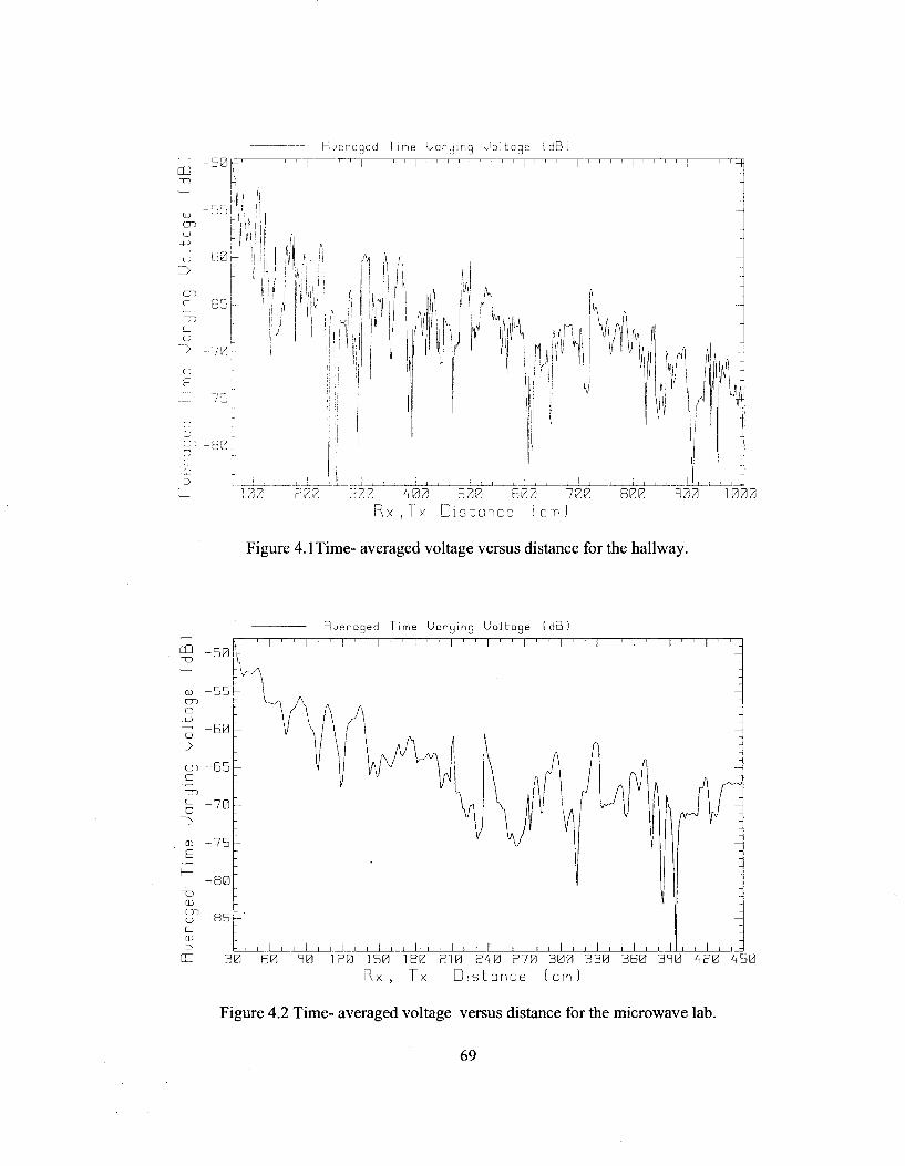
Hueroqed l i m e <J o r q i n q U o l t o g e 1 d B !

- 5 0

100 PZZ 2m 400 500 B00 700 R x . F x LJ1 s t c n c e ( c m )

Figure 4.1 Time- averaged voltage versus distance for the hallway.

( d B )

CE 30 B0 R0 1P0 150 180 £10 ?40 ?70 300 330 360 3^0 4P0 450 Rx, Tx Distance (cm)

Figure 4.2 Time- averaged voltage versus distance for the microwave lab.

69

4.2 Large-Scale Fading

Large-scale fading or slow fading for the signal strength is found by averaging all

the voltage values in a window of width W centered at some distance r along the path.

The window slides along the path as r increases, and the average value within the window

is graphed as a function of r. In the next Section, slow fading is shown for window sizes

ofW = 51.5, 101.5 and 151.5 cm, comparing to 4.8 and 12 X at 2.388 GHz.

4.2.1 Hallway

In the hallway, the field strength was measured at 631 points 1.5 cm apart.

Figures 4.3, 4.4 and 4.5 show the large scale fading with window sizes of 4X, 8 X and 12

X, respectively. Figure 4.3 shows that the 4 X window size effectively eliminates the

fast fading and displays the average value of the received voltage as a function of

distance. Close to the antenna at distances from 85.5 to 141.0 cm, the average received

voltage decreases as the inverse of distance. That is, at 85.5 cm the voltage is -54.74 dB,

and at twice the distance, or 171.0 cm, it is -61.88 dB, for a difference of 7.14 dB. The

ratio of space-free behavior at twice the distance gives a voltage level difference of 6 dB.

The observed value of 7.14 dB for twice the distance is a good approximation. Figure 4.4

with an SX window further suppressed the spatial variation. Figure 4.5 with a 12 X

window shows the field is straight for 150 to 200 cm, constant from 200 to 400 cm and

slightly variable from 400 to 1000 cm.

70

G e ° Ave raged Over D i s t a n c e 5 1 . 5 cm U o l t a g e i n t o o 5 0 - c h m lcod

200 Rx , Tx D i s t a n c e

1000 :m

Figure 4.3Comparison between the point-by-point measured voltage and the voltage averaged over a 51.5 cm ( 4 X) window for the hallway.

o e © flyeroged Over D i s t a n c e 1 0 1 . S cm U o l t a g e i n t o a 5 0 - o h m load

1000

Figure 4.4 Comparison between the point-by-point measured voltage and the voltage averaged over a 101.5 cm (8 X) window for the hallway.

71

Q © o flueroged Ouer D i s t o n c e 1 5 1 . 5 U o l t o q e i n t o a 5 0 - c h m load

E 0 0

R x , T x D i s t a n c e ( c m ) 1000

Figure 4.5 Comparison between the point-by-point measured voltage and the voltage averaged over a!51.5cm(12A) window for the hallway.

4.2.2 Room H853 - Microwave Lab

In the microwave lab, the field strength was measured at 281 points 1.5 cm apart.

Figures 4.6, 4.7 and 4.8 show the large scale fading for the microwave lab, with window

sizes 4, 8 and 12 X, respectively. The received voltage is less variable with distance in

the microwave lab than in the hallway, that is, it shows less small-scale variation. The

window size is not as significant as in the hallway, as can be observed by the very similar

curves for each window size. In other words, changing the size of the averaging window

does not have as much effect as in the hallway. At closer distances the averaged voltage

acts as free space. To verify this, two samples are taken: the second distance twice that of

72

the first, to see if their corresponding averaged voltage value difference is 6 dB. In

Figure 4.6 at distance 55.5 cm the averaged voltage value is -54.02 dB, while at 111.0

cm the averaged voltage value is -59.26 . The difference between the two averaged

voltage values is 5.25 dB which is considered a good approximation for free space.

73

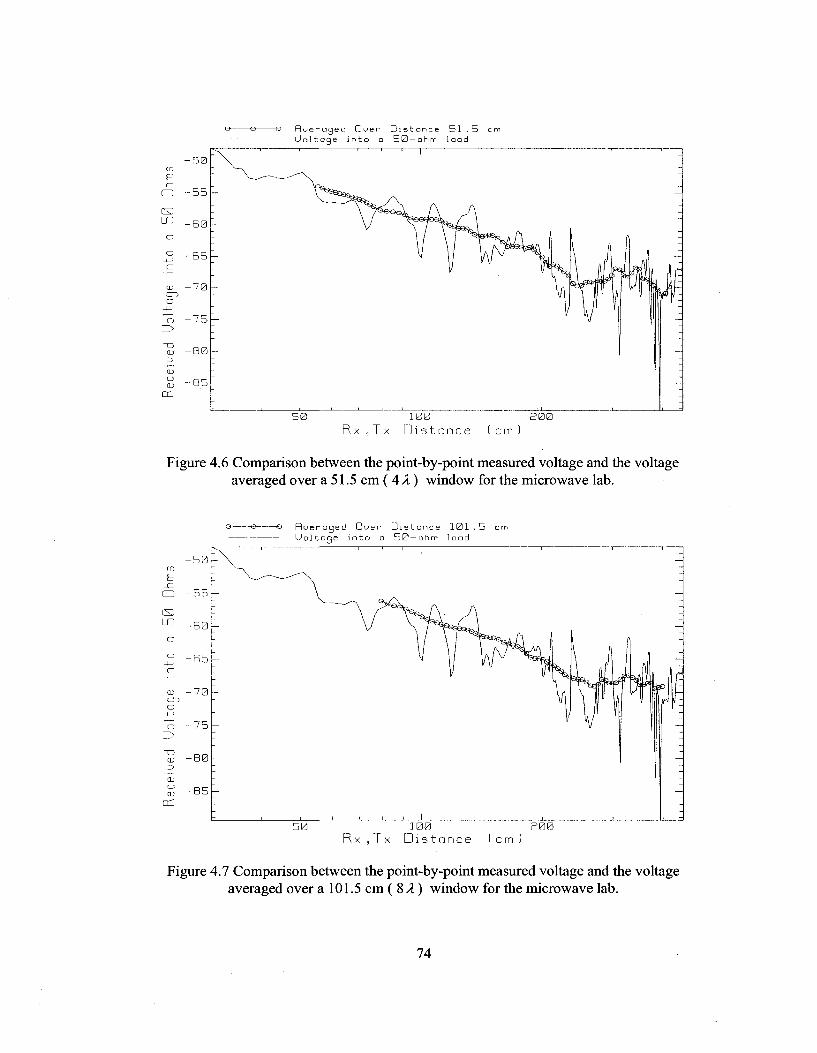
—© R u e r a g e d O v e r D i s t a n c e 3 1 . 5 — U o l t a g e i n t o a 5 0 —ohm l o a d

5 0 100 Rx , T x D i s t a n c e

2 0 0

cm )

Figure 4.6 Comparison between the point-by-point measured voltage and the voltage averaged over a 51.5 cm ( 4 X) window for the microwave lab.

_o Q Rue raged Duer D i s t a n c e 1 0 1 . 5 cm U o l t o g e i n t o o 50—ohm load

5 0 1 0 0 P 0 0 R x . T x D i s t a n c e 1cm)

Figure 4.7 Comparison between the point-by-point measured voltage and the voltage averaged over a 101.5 cm ( 8 X ) window for the microwave lab.

74

—©— o R y e r a g e d Ouer D i s t a n c e 1 5 1 . 5 cm U o l t o g e i n t o a 5 0 ~ o h m lood

O SS\-

1 0 0 £ 0 6 R x . T x D i s t a n c e I c m )

Figure 4.8 Comparison between the point-by-point measured voltage and the voltage averaged over a 151.5 cm ( 12 X ) window for the microwave lab.

4.3 Spatial Variation of the Rician-K Factor

For a given distance between the transmitter and the receiver, all the data points

within a window of width W were taken, extending from (r- W/2) to (r+W/2). This set of

"windowed" data points are then used to calculate the Rician-K factor using the methods

of Chapter 3 to evaluate KGIK24, KMLE and Kn. Three sizes for the sliding window will

be considered, W = 51.5 cm, 101.5 cm and 151.5 cm, which correspond to

approximately 4, 8 and 12 A. The results are given in the following Sections.

75

4.3.1 Hallway

Figures 4.9, 4.10 and 4.11 show the space-varying Rician-K factor as a function

of distance in the hallway for sliding windows of sizes 4/1, 8 X and 12 A respectively.

In Figure 4.9 the curve for KG / K24 (circles) has missing data from 120 to 130 cm and

again from 230 to 280 cm, where the KG formula of (3.5) leads to the square root of a

negative number. Figures 4.10 and 4.11 also have distance ranges where no value of KG

could be found. In Figure 4.9, for Kn (triangles), in some distance ranges such as 110 to

140 cm, 220 to 240 cm and 280 to 320 cm, the root-finding algorithm used to solve (3.9)

clips at about 18 dB. There are similar distance ranges in Figure 4.10 and 4.11. The KMLE

formula (3.14) (crosses) always gives a solution.

In Figures 4.9, 4.10 and 4.11 two distance ranges are observed. The first range is

from 90 cm to 400 cm in Figure 4.9, 110 cm to 400 cm in Figure 4.10, and 130 cm to 400

cm in Figure 4.11. Methods for finding the Rician-K factor do not agree well in the first

range. However, for the second range, from 400 to 980 cm in Figure 4.9, 400 to 945 cm

in Figure 4.10, and 400 to 925 cm in Figure 4.11, the values found by the three methods

correlate well in Figures 4.9 and 4.10. In Figure 4.11 the curve for the KMLE is almost

constant and does not have the large maxima and minima observed with other methods.

76

For the hallway measurement, the KMLE formula is the best tool for evaluating

the Rician-K factor because it found values for every distance between the transmitter

and the receiver. For a window of 4 X, KMLE (crosses) is about 12 dB and shows peaks

and nulls for distances between 90 and 980 cm. For a size 8 X window, KMLE is much

more nearly constant and for a MX window, KMLE is almost constant. Therefore, for a

large window size the Rician-K factor is about the same everywhere in the hallway.

4.3.2 Room H853-Microwave Lab

Figures 4.12, 4.13 and 4.14 show the space-varying Rician-K factor for the

microwave lab. The size of the sliding window is 4 X ,8 X and 12 X, respectively. For

the Kc IK24 method (circles) data is missing between 220 and 260 cm and between 320

and 330 cm in Figure 4.12. In Figure 4 . 1 3 , ^ / ^ 2 4 has missing data at 80 cm and

between 255 and 280 cm. In Figure 4.14, Kc I K2Ahas missing data at 100 cm, between

190 and 210 cm and around 280 cm. This missing data occurs because (3.5) leads to the

square root of a negative number, as was the case in the hallway. The Kn method

(triangles) is clipped at 18 dB by the algorithm used to find the root for (3.9), observable

in the ranges between 220 and 260 cm, 320 and 330 cm and between 370 and 390 cm in

Figure 4.12. In Figure 4.13 this same clipping can be seen between 210 and 240 cm, 250

and 300 cm and between 320 and 360 cm. In Figure 4.14 it is between 108 and 120 cm,

180 and 210 cm, 230 and 250 cm, 260 and 270 cm, 280 and 290 cm, and between 320

77

and 340 cm. The KMLE method, however, finds the Rician-K value for all of the

distances between the transmitter and the receiver.

In Figure 4.12 KMLE values vary with distance, with a large maximum at

165 cm, and a minimum between 220 and 250 cm. KMLE is almost constant between 260

and 420 cm. In Figure 4.13, with an 8 1 window, KMLE is approximately constant

along the path. Figure 4.14 show that with a 121 window KMLE is very nearly constant,

especially from 210 to 360 cm.

The correlation among the three methods for calculating the Rician-K factor is as

follows. The graphs in Figures 4.12, 4.13 and 4.14 all show two regions. The first region

is from 60 cm until 230 cm in Figure 4.12, 80 to 230 cm in Figure 4.13 and from 100

to 230 cm in Figure 4.14 The second region is from 230 cm until the end of the path. In

Figure 4.12 the three curves Kc IK24, Kl2 and KMLE correlate well in the first region. In

Figure 4.13 the three curves correlate less in the first region. In Figure 4.14 there is no

correlation between the curves in the first region. In the second region in Figure 4.12

KG IK24 and Kn correlate recursively but do not agree with KMLE. In Figure 4.13, the

Kl2 method fails over the second region and Kcl K24 does not agree with KMLE. In

Figure 4.14 there is little agreement among the three methods in the second region. As

in the hallway, the KMLE method is the best method to use to find the space-varying

Rician-K factor since it estimates all values of K along the path.

78

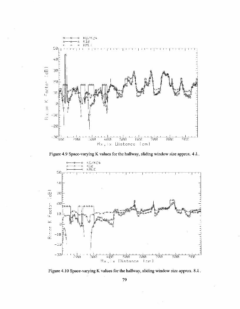
o © o K B / K 2 4 A A A K I P x * * KMLE

-3 ay

> > ' ' I

ft

T ~i—I—i—i—I—I—I—i—I—I—I—|—i—i—I—r

X ±. X _L ]00 200 300 400 500 B00 700 800

Rx,Tx Distance (cm) q 0 0

Figure 4.9 Space-varying K values for the hallway, sliding window size approx. 4 A.

&• © o K D / K 2 4 a A- A K1B x x x KMLE

2 0 0 3 0 0 4 0 0 5 0 0 6 0 0 76 R x , T x D i s t a n c e ( c m )

B00 ^ 0 0

Figure 4.10 Space-varying K values for the hallway, sliding window size approx. 8 A .

79

-o KG/KP4

KMLE

300 4-00 500 600 Rx , Tx Distance ( cm

Figure 4.11 Space-varying K values for the hallway, sliding window size approx.12 A.

CD

cC

60 S0 1B0 150 180 810 840 B70 300 330 360 3S0 4PE R x , T x Distance (cm)

Figure 4.12 Space-varying K values for the microwave lab, sliding window size approximately 4 X.

80

-o KG/KE4 -A K18

-* -x KMLE

85

-30 J i i L J , i L 1£0 150 180 £10 640 £70 300 330 360 33E

Rx ,Tx Distance 1cm)

Figure 4.13 Space-varying K values for the microwave lab, sliding window size approximately 8 X.

-e o KG/KB4 KIB

rv

2 0 0 2 5 0 3 0 0 R x . T x D i s t a n c e ( c m )

.L 3 5 0

Figure 4.14 Space-varying K values for the microwave lab, sliding window size approximately 12 A,.

81

4.4 Conclusions

Large-scale fading is sensitive to the number of points being averaged and to the

variation of the received voltage. For the hallway, it is obvious in Figures 4.3 to 4.6 that

as the size of the window is increased, large-scale fading tends to be less variable.

However, for the microwave lab, increasing the size of the window did not lead to a

significant change in the shape of the curve, as can be seen in Figures 4.6 to 4.8. The

space-varying Rician-K factor is best evaluated using the KMLE method, since this

method estimated all values for K for all of the windows. With a large average window of

12 X, the Rician-K factor estimated by the KMLE method is approximately constant with

distance along the path for both the hallway and the microwave lab, and in both cases has

a value of about 12 dB. In [30] the range for the space varying Rician-K factor had 3.45

as the maximum value, but in this thesis the maximum value found for the Rician-K

factor is 45 dB for the hallway using the KMLE method and 27 dB for the microwave lab

using the three methods mentioned in literature. The results for the Rician-K factor

obtained are significantly different than in [30].

82

Chapter 5

Geometrical Optics Simulation

5.1 Modeling

In this Chapter, ray tracing will be used to simulate the hallway and microwave

lab using the GO_3D program [3]. The received electric field strength will be

calculated for a transmitter with frequency and output power similar to the one used for

the measurements with the site survey system. Note that in the ray-tracing simulation the

transmitter and receiver are interchanged, compared to how they were used in taking

measurements. The transmitter here is at a fixed location and the receiver is moving

along the measurement path. By reciprocity, the received field strength should be the

same.

Also, in the simulation, the transmitting antenna is a half-wave dipole radiating

10 mW. The received field strength will be converted to received voltage as explained in

Section 5.2.

5.1.1 Hallway

Figure 5.1 shows the floor plan of the northwest corner of the 15th floor of the

EV building modeled for analysis of the GO_3D program. The location of the sleeve

dipole and the position of the path corresponds precisely to the measurement scenario.

83

The following dimensions are shown in Figure 5.1. The location of the Tx antenna is in

the center of the hallway 60 cm from the wall behind it. The measurement path initial

distance is 60 cm for the Tx dipole. The path length is 945m. The received signal values

were calculated every 1.5 cm along the path. The Tx is placed 103 cm above the ground

and the Rx is displaced 107 cm above the ground. Transmitting frequency is 2.388 GHz

and the output power is 10 mW.

S45C

Figure 5.1 GO_3D simulated version of the northwest corner of the 15th floor in Concordia's EV building showing the Tx location and the path for the received electric field [39].

84

5.1.2 Room H853 Microwave Lab

Figure 5.2 shows a simulated version of the microwave laboratory with

representation of some equipment, showing all of the dimensions of the measurement

setup. The transmitting dipole is 90 cm from the nearby lab bench, labeled in the Figure

"wood table". The path starts 30 cm from the dipole and has a length of 450 cm. The

path is in the middle of the space between the two benches. The Tx is 103 cm above the

ground and the Rx is 107 cm above the ground. The transmitting frequency is 2.388 GHz

and the output power is 10 mW.

J/_

Metol

Drouers

rtttol

J/c

-Tf, T

75cm

K > _^

K — N

Figure 5.2 GO_3D simulated version of the microwave lab showing the Tx location and the path for the received electric field.

85

5.2 Voltage in dB versus Position

The GO_3D program calculates the amplitude of Ex, E , and E, at every point

along the path. These are combined to get the "total" electric field amplitude Et using

^ = v i ^ r + N 2 + K - i 2 - (5-1)

The total electric field values are transformed into received voltage across a 50-

ohm load in dB for comparison with measured received voltage values. The following

formulas were used to make the transformation. The amplitude of the total electric field

strength computed by GO_3D is converted to an RMS value using

Erms = ^ (5.2)

where Eampl is the amplitude of the total electric field strength computed by GO_3D, and

Erms is the RMS value of the total electric field strength.

86

The RMS value of the electrical field strength is transformed to dB using

EdB=20logl0Erms (5.3)

where EdB is the electric field strength in dB, relative to 1 V/m field strength.

To transform the electrical field strength in V/m to voltage in dB, a parameter

known as the Antenna Factor (1/m) must be found for the Rx antenna. This is found

using [25]

AFdB =201og1 0(/)-Gd B ,-149.8 (5.4a)

where the frequency / is in Hz, or equivalently

AFdB = 20logl0(fMH:)-GdBi-29.8 (5.4b)

where the frequency fMH. is in MHz and is 2388 MHz in this thesis. In these equations,

AFdB is the antenna factor in dB, and Gm is the gain of the receiving antenna, which is

1.83 dB, obtained from the specification sheet of the sleeve dipole used in the

measurements.

87

From the antenna factor in dB and the electric field strength in dB, the voltage

received in dB can be found from

VdB=EdB-AFdB (5.5)

where VdB is the voltage received in dB.

The voltage received in dB is transformed to linear scale by the following:

V = 10 20 (5.5)

where V is the voltage in linear scale.

Thus, the GO_3D program reports E ,, which is converted to EdB using eqs.

(5.2) and (5.3). Then EdB is converted to voltage VdB using (5.4) after the antenna factor

is found from (5.3).

88

5.2.1 Comparison of Measurement and Simulation Results

When comparing measured results with the simulated data from G 0 3 D , it must

be noticed that the output power of the transmitter in the simulation is assumed to be 10

mW. For the measurement results this was not the case because the actual power radiated

is not known. The output power of the circuit in the transmitting unit was measured to be

10 mW into a matched load. But the input impedance of the monopole on the transmitter

unit is not known, so the actual radiated power is not known [24]. The measured voltage

needs to be calibrated to be the same voltage level as the simulated data. This has been

done by multiplying the measured data on a linear scale by the linear ratio of the average

value of the simulated voltage to the average value of the measured voltage.

5.2.1.1 Hallway

Figure 5.3 shows the simulated and calibrated measured voltage for the hallway.

The fast fading of the simulated voltage does not match the measured voltage very well.

Also, [40] shows that the accuracy of the results of a ray-tracing simulation are greatly

enhanced if the electrical parameters of the wall materials are measured directly. But in

the ray-tracing model used in this thesis the electrical parameters were found from the

literature and it is not known if they are a good representation of the actual walls in the

hallway.

89

Another possible reason for the considerable difference between the measured

data and the simulation in Figure 5.3 is the construction of the walls in the 15th floor

hallway. The ray-tracing model represents the walls as constructed of uniform layers of

materials. But the actual wall construction is gyproc sheets about 1 cm in thickness,

supported by vertical metal studs with approximately 16 cm spacing. The wall

construction is poorly modeled by a uniform layered structure. Instead the metal studs

may behave as a secondary source, and this cannot be modeled in the GO_3D program.

5.2.1.2 Room H853 microwave lab

Figure 5.4 shows the simulated and calibrated measured data for the microwave

lab. The data shows a good match between the simulated and calibrated measured data

from 30 cm to 140 cm, and a reasonable match up to 240 cm. A possible reason for the

good match is the detailed representation of the microwave lab in the GO_3D program.

There is a marked difference in the region between 240 and 330 cm. Eventually, at

about 400 cm, the walls in the microwave lab behave as uniform layered structures.

90

S i m u l a t e d M p. a s 11 r e ri

i — | — i — i — i — i — | — i — i — i — i — | — i — i — i — i — | — i — i — i — i — | — i — i — i — i — | — i — i — i — i — | — i — i — i — i — | — i — i — i — i — | — i — i — i — i — i

100 £00 300 400 500 600 700 800 ^00 1000 Rx , Tx Distance ( cm )

Figure 5.3 Simulated and calibrated measured results of voltage in (dB) versus distance for the hallway.

- 3 0

QD

aj en o

S imu la ted Measured

1 I ' ' I ' ' I ' ' I ' ' I ' ' I ' ' I ' ' I

I I I I ! I I , , I

30 60 T0 180 150 180 810 840 870 300 330 360 3=10 480 450 Rx , Tx Distance [ cm )

Figure 5.4 Simulated and calibrated measured results of voltage in (dB) versus distance for the microwave lab.

91

5.3 Path loss Index ' « "

The path loss index is a parameter used to describe the variation of the large-scale

variation of the received voltage over distance. The path loss index n is calculated

from measured data in the following manner [24]. The power law model on a

logarithmic scale is

r*=20.1od rn (5.6)

Rearranging results in

K<B=201ogK0-/i.201ogri. (5.7)

(5.7) is the equation for a straight line

y: - b + mxj (5.8)

where yi = VdB ,b = 201ogF0 =VdB0 ,b = -n and xi = 201ogr ;.

92

Using the method of least square error which assumes that the square of the sum

of the difference between the measured value of data and the straight line is to be

minimized. Q is presumed to be the difference between the measured data VdB and the

straight line yi -b + mxi. If m is the number of points of measurements, then Q is given

by

m

Q = S K, - (VdB0 - n20 log rt ))2 (5.9)

1 = 1

To find the values of VdB0 and n that make Q minimum, take the partial

derivative of Q with respect to VdB0 and set it equal to zero, and take the partial

derivative of Q with respect to n and set it equal to zero. This results in two linear

equations with two unknown quantities; VdB0 and n . Solving the two linear equations

for Vdm and n in terms of the other quantities results in

m m m

£K<ff l /£201og(r /)-i«£K<ff l /201og(r /) n = ± 1 ^i w

mX(201og(r,))2-l£201o8(';)J

and

m m

J>«+»Z201°8(l)

The full derivation for (5.10) and for (5.11) is in Appendix E.

(5.10)

(5.11)

93

5.3.1 Comparing Measurement and Simulated " n " Values

This Section compares the path loss index n of the measured and simulated

voltages. It gives an indication of whether the received signal declines with distance in

the same manner for measured and simulated data. In other words, this gives an insight

into how much the simulation and measured data agree based on the path loss index n .

5.3.1.1 Hallway

Figure 5.5 shows the simulated and uncalibrated measured received voltage

graphs for the hallway. The path loss index n is 0.7503 for simulated data and 0.6847

for measured data. The measured and simulated data did give a good agreement, based on

the path loss index n. Although the detailed variation or fast fading differ considerably,

the path loss index is quite similar.

5.3.1.2 Room H853 Microwave Lab

Figure 5.6 shows the simulated and uncalibrated measured received voltage

graphs for the microwave lab. The path loss index n is 0.8676 for simulated data and

0.9187 for measured data. Based on the similarity of the n values, we can conclude that

the measured and simulated data give good agreement and that the simulation model is a

reasonably good model. It is of interest that the path loss index n is much higher in the

microwave lab, at about 0.9 than in the hallway at about 0.7.

94

- Simulated Pothloss Index — Simuloted data -o Measured data

Measured Pathloss Index

0 . 7 5 0 3

. 6 8 4 7

D i s t a n c e ( cm )

Figure 5.5 Simulated and measured results of voltage in (dB) versus distance for the hallway showing path loss index n .

CD

en - 6 0

7 3

- 8 0

S i m u l o t e d P a t h l o s s I n d e x n = 0 . 8 6 7 6 S i m u l a t e d d o t a M e a s u r e d d a t a M e a s u r e d P o t h l o s s I n d e x n = 0 . ^ 1 8 7

—, . i T -i -[ r

100 Rx , Fx D i s t a n c e ( c m

£ 0 0

Figure 5.6 Simulated and measured results of voltage in (dB) versus distance for the microwave lab showing path loss index n .

95

5.4 Large-Scale Fading

The large scale fading for measured and simulated results is compared in this

Section. As in Chapter 4, the sliding window concept is used and three window sizes are

considered. The window sizes used was 4 A, 8 A and 12A. The next sub Sections

present the large scale fading for measured and simulated data for the hallway and the

microwave lab, along with supporting Figures.

5.4.1 Hallway

Figures 5.7 to 5.9 show large-scale fading for measured and simulated data of the

hallway for window sizes 4A, SA and \2A, respectively. In Figure 5.7, with window

size 4A, at closer distances between the transmitter and the receiver, or the free space

behavior, there is clearly a good match between measured and simulated data.. At

distances from 300 cm till the end of the path being measured, or 1000 cm, there is a

marked difference between measured and simulated data. In Figure 5.8, with window size

8 A, the free space region matching is even better than in Figure 5.7. At distances after

the free space region or from 300 cm until the end of the path, there is a similar

difference between measured and simulated data. The data in Figure 5.9, with window

size 12A, is similar to that of Figure 5.8 but the free space region matching is even

better. All three Figures share in common the free space behavior with good matching

between the measured and simulated data, and a second region with very little matching.

This is also obvious in the small-scale fading.

96

S i m u l a t e d , w i n d o w s i z e 5 1 . 5 c r

O

(X) L D

D

O -J-> C

CD c n O

z>

CD O tu

cc

4 0

4 5

5 0

5 5

G & -

\ ^

\

-

-

_ _ i _ _ . 1

— © M e a s u r e d w i n d o w s i z e b l .b c m

-

-

\ jr» %| \-

\ / 1

100 200 R x , T x D i s t a n c e I cm )

500

Figure 5.7 Large-scale fading (measured and simulated ) for the hallway, window size around 4 A,.

— S i m u l a t e d , w i n d o w s i z e 1 0 1 . 5 cm -© M e a s u r e d , w i n d o w s i 7 e . 1 0 1 . 5 cm

-CZ

CD

IS)

- 4 0 .

£ 0 0 R x , 1 x D i s t a n c e

Figure 5.8 Large-scale fading (measured and simulated ) for the hallway, window size around 8 X.

97

S i m u l c t e d , w i n d o w s i z e 1 5 1 . 5 cm Q Q o M e a s u r e d , w i n d o w s i z e 1 5 1 . 5 cm

CD E

J C CD

( S m

D

O - 1 - ^ c

CD ro D

o Z>

" O CD 3

CD O a)

ai

- 4 0

( - 4 E

- 4 4

- 4 6

- 4 8

- 5 0

- 5 £

£ 0 0 5 0 0 Rx , I x D i s t a n c e 1 c m )

Figure 5.9 Large-scale fading (measured and simulated) for the hallway, window size around 12/1.

5.4.2 Room H853- Microwave Lab

Figures 5.10 to 5.12 show the large scale fading for the simulated and scaled

measured data of the microwave lab, for window sizes 4 1 , 8 1 and 1 2 1 , respectively.

In Figure 5.10, for window size 4 1 , at closer distances between the transmitter and the

receiver there is a very good match between measured and simulated data. From 250 cm

until the end of the path there is a notable difference between measured and simulated

data. In Figure 5.11, for window size 8/1, the results are very similar to those in Figure

5.10. In Figure 5.12, for window size 1 2 1 , there is a good match between the measured

and the simulated data until 300 cm. From 300 cm until the end of the path matching is

less. The large scale fading matching for measured and simulated data for the microwave

lab is similar to the small scale fading matching.

98

100 &B0

R x , T x D i s t a n c e ( c m )

Figure 5.10 Large-scale fading (measured and simulated) for room H853, window size around AX.

S i m u l a t e d . w i n d o w s i z e 1 0 1 . 5 cm © © G M e a s u r e d ,Luindotu s i z e 1 0 1 . 3 cm

1 0 0 P 0 0 R x , T x D i s t a n c e ( c m )

Figure 5.11 Large-scale fading (measured and simulated) for room H853, window size around 8 A.

99

3 i r n u l a t e d , L u i n d o u j s i z e 1 5 1 . 13 c m

B00 R x , T x D i s t a n c e 1 c m ]

Figure 5.12 Large-scale fading (measured and simulated) for room H853, window size around 12 A.

5.5 Spatial Variation for the Rician-K Factor

In this Section, the space-varying Rician-K factor for the simulated data is

estimated using the three methods mentioned in Chapter 3, which are KG IK24, Kn and

KMLE. The window sizes are 4, 8, and 12 A. Subsequently, the best method to evaluate

the Rician-K factor is determined and then compared with its equivalent found from the

measured data.

100

5.5.1 Hallway

Figures 5.13 to 5.15 show the space-varying Rician-K factor for the hallway. The

window sizes are 4, 8, and 12 A, respectively. In Figure 5.13 the values of the three

methods KG/K24 (circles), Kn (triangles) and KMLE (crosses) correlate well except

between 430 cm and 480 cm for Kn (triangles), where values for the algorithm used to

search for the root of (3.9) are clipped at around 18 dB. Between 800 and 820 cm there

are missing values in the KG IK24 curve. These values are the square root of a negative

number in (3.4). The Rician-K factor is highly variable with a maxima at about 500 cm

and a minima at about 450 cm. In Figure 5.14 the correlation between the three

methods is better than in Figure 5.13 but with two clippings: at 400 to 440 cm and from

800 to 840 cm. The Rician-K factor is less variable than in Figure 5.13 with a maxima at

900 cm. In Figure 5.15 the Rician-K factor is nearly constant at around 12 dB. There are

regions from 320 to 460 cm where the Rician-K factor is clipped by the algorithm used

to find the root for (3.9) with the Kn method and missing data for the Kc IK24 method

between 440 and 460 cm where (3.4) gives root squares of a negative number. The

correlation between the three methods is much less here than in the other two Figures.

The KMLE method appears to be the best to find the Rician-K factor for space-varying

simulated data' since it found all the Rician-K factor values along the distance. For the

simulated data, all three methods agree very well.

101

-o KG/K24 -A K12 --* KMLE

CD

1_ O

CJ O

c o u

or:

200 300 400 500 600 700 R x . T x D i s t a n c e ( c m )

Figure 5.13 Space-varying K for the hallway, window size around 4 A .

o e o KG/K24

80

-* K12 -* KMLE

" i—i—i—i—r ~i—i—!—r"

CD ~ 0

t_ O

D LL

^

c o o

cr

7 0

6 0

5 0

4 0

3 0

2 0

10 C

. 0

- 1 0

- 2 0

-30

T

_L X ! , I I . . 200 300 400 500 600 7E

R x . T x D i s t a n c e ( c m ) R00

Figure 5.14 Space-varying K for the hallway, window size around 8 A .

102

o e e KG/K24 & A A KIP x * x KMLE

300 400 500 B00 IV Rx , Tx Distonce ( cm )

S00

Figure 5.15 Space-varying K for the hallway, window size around 12 A.


Figures 5.16 to 5.18 show the space-varying Rician-K factor for the microwave

lab. The window sizes are 4, 8, and 12 A, respectively. In Figure 5.16 the three methods'

values are not correlated at all except in the regions between 160 and 210 cm and 320 to

390 cm. Clipped values are found for the Kl2 method at regions between 120 and 150

cm, 230 to 320 cm, and 310 to 410 cm. Missing data are found for the KG /K24 method

because (3.4) gives the root square of a negative number at certain distances. Here, that

range is from 270 cm to 290 cm. The Rician-K factor is highly variable with a maximum

103

at 280 cm and a minimum at 230 cm. In Figure 5.17, correlation between the three

methods is even less than in Figure 5.16, aligning only at the region between 345 cm and

400 cm where the values for two methods, KG IK24 and Kn correlate. The Kn method

is clipped at 135 cm, from 140 to 150 cm and from 230 to 330 cm. The KG IK24

method has missing data (root square values for a negative number) in the region from

240 to 320 cm. In Figure 5.18 the Rician-K factor is clipped at 8 dB using the Ku method

for almost all the distance path. The Rician-K factor has missing data for the KG IK24

method (root square values for a negative number) in the regions 100 to 110 cm, 160 to

180 cm and 260 to 340 cm. The Rician-K factor found using the KMLE method is

constant along the path being measured, and it has a value of about 2 dB. The KMLE

method is clipped at 0 dB from 250 to 310 cm. Observing Figures 5.13 to 5.17, it is

clear that the KMLE method is the best method to find the Rician-K factor. In the next

Section, comparison between the space-varying Rician-K factor for measurements and

for simulation is presented for the KMLE method since it is the best method in both cases.

104

50

K G / K 2 4 A A A K 1 2 x x x KMLE

CD

c o

4-> O o

Li_

C D

en

30

-20A

T T I ' ' I ' ' I ' ' I ' ' I ' ' I ' ' I ' ' n

_L J_ _L _L J_ J_ JL _L JL J _ J _

60 S0 120 150 1B0 310 340 270 300 330 3B0 3S0 430 R x , T x D i s t a n c e ( c m )

Figure 5.16 Space-varying K for room H853, window size around 4 X.

© e o K G / K 2 4 -& A K13 - * x KMLE

CD

o u o

c o

o

- 3 0

I ' ' I ' ' I ' ' I

± I . i I . I i i I JL_3

I 130 150 180 310 340 370 300 330 360 310 R x , T x D i s t a n c e ( c m )

Figure 5.17 Space-varying K for roomH853, window size around 8 A.

105

50

CD

— 30

u o

c D

U

cr

Q e o KG/K24 A A A K I P x x x KMLE

20

- 1 0 h

-20 J L_

150 200 250 300 Rx , Tx Distance ( cm )

350

Figure 5.18 Space-varying K for room H853, window size around 12 X .

5.6 Comparison of Simulated and Measured K MLE

The space-varying Rician-K factor for the hallway and microwave lab simulated

data was evaluated using the three methods: KG /K24, Kl2 and KMLE. The best method

to use for evaluating the space-varying Rician-K factor from simulated data is the KMLE

method since it evaluates K for all distances along the path being measured. Since this is

the case for measured data also, KMLE curves for measured and simulated data can be

compared. Figures 5.19 to 5.24 show the comparison between the KMLE curves for the

measured and simulated data, in the hallway and in the microwave lab for three window

sizes 4, 8 and 12 A .

106

5.6.1 Hallway

Figures 5.19, 5.20 and 5.21 show the space-varying Rician-K factor for measured

and simulated data for the hallway, estimated using the KMLE method and at three

different windows sizes: 4, 8 and \2X.

In Figure 5.19, for a window size of A A, there is no correlation between the KMLE

-generated Rician-K factor from measured and simulated data. The average KMLE values

from measured data is 14.85 dB, and 24.74 dB from simulated data. The average value

for KMLE from simulations in dB is about twice that from measurements. For Figure

5.20, with an 8 A window size, the correlation is better than in 5.19. The average value

for KMLE from measured data is 12.83 dB, and from simulated data, 16.93 dB. Figure

5.21 with window size 12/1 shows a correlation better than that of Figure 5.20. The

average value for KMLE from measured data is 12.23 dB, and for simulated data, 13.98

dB. The three graphs show that at the 12/1 window size the KMLE average value from

simulations is within 2.2 dB of the measurements, which is a reasonable match. The

average values produced for the above graphs are found from the linear scale of the data

and then taking the db value of each. Also, with a large window size, KMLE is

approximately constant along the path, especially for the measured data.

107


Figures 5.22, 5.23 and 5.24 show the space-varying Rician-K factor for measured

and simulated data for the microwave lab estimated using the KMLE method and at

different windows sizes: 4, 8 and 12 A.. In Figure 5.22, with window size 4X, the KMLE

curves found from measured and simulated data are somewhat correlated except in the

region from 230 cm to 320 cm. The average KMLE from measured data is 12.84 dB, and

from simulated data KULE is 11.07 dB, which are almost identical. In Figure 5.23, with

window size 8 X, KMLE curves have almost identical behavior, with average values of

11.39 dB for measurements and 8.60 dB for simulations. Figure 5.24 with window size

12/1 shows that the behavior is almost constant, and KMLE has an average value of

10.15 dB for measured data and 7.026 dB for simulated data. Note that especially for the

larger window size, KMLE is nearly constant with position along the path. The simulated

data has ranges of distance where the KMLE algorithm returns to near-zero values in dB

which corresponds to small values in a linear scale. There is significant variation in the

signal of Figure 5.4 from 240 cm to 320 cm. This results in a small value for the Rician-

K factor and thus justifies the small values obtained.

108

KMLE Simulated KMLE Measured

100 200 300 400 500 600 700 800 S00 R x , T x D i s t a n c e ( c m )

Figure 5.19 Space-varying K comparison for the hallway, window size around 4 A.

KMLE Simulated KMLE Measured

B00 300 400 500 600 700 R x , T x D i s t a n c e ( c m )

8 0 0 ^ 0 0

Figure 5.20 Space-varying K comparison for the hallway, window size around 8/1

109

KMLE Simuloted x * x KMLE Measured

4 0 0 5 0 0 6 0 0 7 0 0 R x , T x D i s t a n c e ( c m )

B 0 0 S 0 0

Figure 5.21 Space-varying K comparison for the hallway, window size around 12 X.

CD

^ SB\-

K M L E S i m u l a t e d K M L t M e a s u r e d

6 0 S0 120 150 1 8 0 310 2 4 0 2 7 0 3 0 0 3 3 0 3 6 0 3 9 0 4 2 0 R x , T x D i s t a n c e ( c m )

Figure 5.22 Space-varying K comparison for room H853, window size around 4X.

110

5 0

CD

^ 2

o

or

KMLL Simuloted - * KMLE Measured

^0 120 150 1B0 210 240 270 300 330 3B0 3R0 R x , T x D i s t a n c e ( c m )

Figure 5.23 Space-varying K comparison for room H853, window size around 8/1.

4 0

3 0

^ 2 0

0 k-

K M L E M e a s u r e d KMLE Simulated

3 5 0 x D i s t a n c e ( c m )

Figure 5.24 Space-varying K comparison for room H853, window size around 12 A.

I l l

5.7 Conclusions

The following is observed when comparing results obtained from measured and

simulated data. The measured small-scale fading for the hallway does not match the

simulations as shown in Figure 5.3. The ray-tracing model representing the hallway walls

is a uniform layered structure, which is probably not a reasonable model. The hallway

walls are constructed from vertical metal studs spaced 16 cm each, covered with gyproc

panels about 1 cm thick. The metal studs should be modeled with the uniform-layer

representation. They act as secondary sources. In the microwave lab the matching

between measured and simulated small-scale fading results as shown in Figure 5.4 is

better due to proper representation of the microwave lab environment. One reason for the

differences between measured and simulated small-scale fading results for both the

hallway and the microwave lab might be that the ceiling in the simulation is modeled as

perfectly smooth and as reflecting the signal specularly. The reality is that above the

hanging ceiling, there are pipes, ducts, electrical conducts and so forth which scatter the

signal rather than reflect it specularly, and this is not modeled in the simulations. Some

researchers "calibrate" the wall model chosen, the electrical parameters of the wall

matched so that the calculated slow fading matches the measured slow fading for some

paths. Then the "calibrated" model is used to calculate the calculate the slow fading and

path loss for many other paths. After calibration the match between simulation and

measurements is greatly enhanced. Large-scale fading in the hallway was a poor match

between the measured and simulated data, but was a reasonable match in the microwave

lab. When comparing measured and simulated data based on the path loss index n for the

112

hallway and microwave lab, there is good agreement for the path loss index generated

from measured and simulated data. The path loss index is higher in the hallway than in

the microwave lab. Reference [24] shows that the path loss index is dependant on the

location of the path being measured, and reference [12] shows that the path loss index is

directly proportional to the height of the transmitter. Hence, if the measurements had

been done at a different height and a different spacing, a different value of the path loss

index n would have been found. The KMLE method is the best to find the space-varying

Rician-K factor. Measured and simulated curves for the KMLE method using three

window sizes have been compared for the hallway and the microwave lab. The

comparison showed that the Rician-K factor becomes independent of position with large

window sizes. The situation of large-scale fading and representation using the log-normal

distribution [7][35] has not been investigated in the thesis.

113

Chapter 6

Conclusions and Future Work

6.1 Highlights

A site-survey measurement system has been built and is described in Chapter 2. It

has the advantage of being automated so that only one operator is needed to operate the

system and to monitor the measurement campaign. The spectrum analyzer and the

moving platform are controlled in sequence by one control unit ( the pc unit ) using

Lab VIEW programming. Space and time power variation measurements for two different

geometrical environments, an empty hallway and a heavily-equipped microwave lab

room, were performed using the site survey system.

In Chapter 3, time variation of the received signal for four representative distance

points in the hallway and for the microwave lab were shown. Three methods from the

literature were used to find the Rician-K factor for time-varying received voltages. Figure

3.18 for the hallway and Figure 3.19 for the microwave lab show that the KGIK14

method is the best means to find K since it is able to find a value for K at every point

along the distance path being measured. In Figure 3.9 for the hallway and Figure 3.20 for

the microwave lab, and the corresponding Rician-K factor Figures for the hallway and the

microwave lab, small time variations of the received signal correspond to a high value of

114

K, corresponding to an almost deterministic voltage. But higher time variations of the

received field corresponded to smaller values of K.

Space variations for the hallway and the microwave lab are found in Chapter 4 by

taking the average value of the time-varying voltage at each distance point along the path

being measured, as shown in Figure 4.1 for the hallway and Figure 4.2 for the

microwave lab. Large-scale fading for the hallway and the microwave lab is investigated

using three averaging windows of sizes 4, 8 and 12 A, shown in Figures 4.3 to 4.5 for the

hallway and Figures 4.6 to 4.8 for the microwave lab. The space-varying Rician-K factor

is found using the same three methods that were used to find the time-varying Rician-K

factor. Three different window sizes, of 4, 8 and 12 A, are considered, as shown in

Figures 4.9 to 4.11 for the hallway and Figures 4.12 to 4.14 for the microwave lab. The

best method for estimating the Rician-K factor for space variation is the KMLE method.

In Chapter 5, small-scale fading for the calculated simulated voltages versus

distance for the hallway and the microwave lab is compared with the corresponding

calibrated and measured space-varying voltages versus distance, shown in Figure 5.3 for

the hallway and in Figure 5.4 for the microwave lab. The comparison shows that there is

poor agreement for the small-scale fading in the hallway and better agreement in the

microwave lab. The large-scale fading for the calibrated measured and simulated

voltages for the hallway and the microwave lab was found using three window sizes of 4,

8 and \2A, shown in Figures 5.7 to 5.9 for the hallway and Figures 5.10 to 5.12 for the

microwave lab. There is better agreement in the microwave lab between measured and

115

simulated large-scale fading than in the hallway. The space-varying Rician-K factor for

the simulated data is estimated using the same methods for the measured data shown in

Figures 5.13 to 5.15 for the hallway and Figures 5.16 to 5.18 for the microwave. The

KMLE method is the best method used to estimate the Rician-K factor for the space

variations. The KMLE curves for space-varying measured and simulated data are

compared in Figures 5.19 to 5.21 for the hallway and Figure 5.22 to 5.24 for the

microwave lab. In these Figures it is clear that as the window size increases, the Rician-K

factor becomes constant with distance.

6.2 Contributions of the Work

The contributions of the thesis are described in the following Sections.

6.2.1 Site-Survey System

The robot used in the site survey system was designed and built by the author.

The robot is a substantial improvement over the one in [24] in terms of wireless control

and automated measurements. In [24] the fixed antenna on the tripod is the transmitter

and the moving robot carries a receiver antenna. A cable is used between the robot and

the spectrum analyzer. As the robot moves the cable trails behind it. The site survey

system in this thesis eliminates the trailing cable. Also in [24] the robot was moved

manually by one distance step, and the power received by the spectrum analyzer was

recoded by the operator on paper. Hence to measure the power at 600 locations, the

116

system in [24] required the operator to move the robot manually 600 times and to write

down the measured received power 600 times. These problems have been overcome by

the site-survey system described in Chapter 2. The robot carries a battery-operated

transmitter and no trailing cable is needed. Commands to move the robot are sent over a

900 MHz wireless channel, rather than manually. The receiver is fixed on a tripod

connected by a short cable to the spectrum analyzer. The wireless command channel at

900 MHz does not interfere with the wireless channel for measurements, which is at the

ISM band frequency of 2.4 GHz. The 900 MHz channel and its corresponding

harmonics, second harmonic 1.8 GHz and third harmonic 2.7 GHz, do not lie within the

band of the measurement wireless channel. The power received by the spectrum analyzer

is recorded automatically at each point by the controlling program and written to a text

file, which will be saved on the computer. The site survey system described in Chapter 2

has total automation, with no need for manual intervention even for long distances being

measured. The drawbacks in this site-survey system are that the robot does not follow

corners and sometimes it gets stuck between the grooves in-between the floor tiles. The

battery life-time needs to be improved. It would be better to use one source for the whole

system to power the mobile platform, instead of three different sets of batteries.

6.2.2 Time-Varying Measurements and Rician-K Factor

The Rician-K factor for the time-varying voltages is better estimated using the

KG IK24 method. High values of the time-varying Rician-K factor correspond to small

time variations of the received voltage. Low values of the Rician-K factor correspond to

117

received voltage values that show some variation over time. The varying values of

voltages received over time are likely due to movements of people in the vicinity of the

measurement environment. Hallway results in Figure 3.9 show more varying voltage

values received compared to the microwave lab in Figure 3.17.

6.2.3 Space -Varying Measurements and Rician-K Factor

The investigation of the space variation using the measured data showed that the

Rician-K factor values are much smaller than those for time variation, and that the

KMLE method is the better method to use to estimate the value of space-varying Rician-

K factor. It was found that for a large window size, 12 A, shown in Figure 4.11 for the

hallway and in Figure 4.14 for the microwave lab, the KMLE estimate of the Rician-K

factor is approximately constant all along the path.

6.2.4 Simulations

The measured and simulated results were compared to see if the ray-tracing

model is a good representation of the real environments. The comparison was based on

small-scale fading, path loss index n, large-scale fading and the KMLE curves for both

measured and simulated data. The small-scale fading in the hallway agreed poorly

between the measurements and simulations. The agreement was much better in the

microwave lab. The layered model for the wall is a poor representation of the gyproc and

118

metal studs construction of the hallway walls. The large-scale fading was compared on

the basis of path loss index n, and there was good agreement for both the hallway and

the microwave lab. The microwave lab gave a higher value for n . The large-scale fading

for both measured and simulated data gave a good match in the free space region. For the

Rician-K factor estimated by the KMLE method, it was found that as the size of the

window increases, KMLE becomes more constant along the path. This is shown in Figure

5.21 for the hallway and in Figure 5.24 for the microwave lab, both for window size

12A.

6.2.5 Validation of The Methods For Evaluating the Rician-K Factor

Figure 3.19 shows that the three methods used to estimate the value of the

Rician-K factor give the same values of K at many points, for example from 250 to 270

cm, and also from 380 to 400 cm. This indicates that the algorithms used to evaluate

KG/K24, K]2and KMlE are correctly implemented. However, when the data leads to

large values of Kn and KMLE, the root-finding algorithm is not adequate and the large

values are clipped. A better root-finding algorithm should be found, capable of

calculating large values. Also Figure 5.23 shows that the KMLE method returns a zero

value from 245 to 310 cm distance, which is clearly incorrect. The algorithm should be

improved to overcome this shortcoming.

119

6.2.6 The Three Methods For Evaluating The Rician-K Factor

In this section, the advantages and disadvantages of the three methods used in

this thesis to estimate the value of the Rician-K factor are discussed. The advantages for

the three methods are as follows. KGIK24 is evaluated with a simple, closed-form

formula. For the nearly-constant temporal data in Chapter 3, the formula always gives a

value for this high-K case. Conversely, for the rapidly-varying fast fading presented in

Chapter 4, the KMLE method always gives a value for this low-K case. The values

obtained with the Kn method match the KG IK2A values well, but Kn is much harder to

evaluate. The Kn method has the advantage that it obtains values over some ranges of

distance where the KG /K24 method fails in Figs. 4.9 and 4.10. The disadvantages for

the three methods are as follows. The KG IK24 formula sometimes leads to the square

root of a negative number for spatial variations, and so the formula fails. The KMLE

method poorly matches the other methods for high K values, and the implementation

used here suffers from clipping. The KMLE method requires root-finding and is hard to

implement. The implementation in this thesis led to both clipping and zero values for

some of the spatial data. Also, KMLE agreed poorly with the KG I K2tt and Kn methods

for spatial data. The disadvantage of the Kn method is that it is also difficult to evaluate

because it requires a root-finding algorithm. Kn agrees reasonably well with KG /K24

for spatial data in Figs. 4.9 and 4.10.

120

6.3 Recommendations for Future Work

Future work would include more extensive measurements and investigation of

the Rician-K factor for different scenarios. This could be done by additional

measurements for the same environment but with different setups, such as varying the

height of the transmitter and the receiver, and using different frequencies and different

polarizations. Investigating different numerical root finding methods might lead to better

results for KMLE. Some investigation should be done on how to properly model the walls

in the GO_3D program in order for a particular environment to be simulated. This is an

essential issue to ensure that the simulated data matches the measured data and that the

ray-tracing based GO_3D program can be used as an alternative to measurements for a

quick investigation of the wireless channels of certain indoor environments.

121

References

[1] Dobkin D. M., " RF Engineering for Wireless Networks Hardware, Antennas, and

Propagation," Elsevier Publishing, Amsterdam, 2005, ISBN 0750678739.

[2] Sarkar T. K., Ji Z., Kim K., Medouri A., Salazar- Palma M., "A Survey of

Various Propagation Models for Mobile Communication," IEEE Antennas and

Propagation Magazine, Vol. 45, No. 3, pp. 51- 82, June 2003.

[3] Trueman C.W., "Three Dimensional Geometrical Optics Code for Indoor

Propagation," Applied Computational Electromagnetics Society Journal, Vol.17,

No.2, pp. 134- 144, July 2002.

[4] Trueman C.W., "User's Guide for Program GO_3D, Version IK," Concordia

University, November 16 1998.

[5] Rappaport T.S., "Wireless Communications Principles and Practice," Prentice

Hall Publishing, Upper Saddle River, New Jersey, USA, 1996, ISBN:0-13-

375536-3.

[6] Anderson J. B., Rappaport T.S., Yoshida S. "Propagation Measurements and

Models for Wireless Communications Channels," IEEE Communications

Magazine, Vol. 33, No. 1, pp.42-49, January 1995.

122

[7] Hashemi H. "The Indoor Radio Propagation Channel," Proc. of the IEEE, Vol. 81,

No.7, pp. 943-968, July 1993.

[8] Hall M.P.M., Barclay L.W. and Hewitt M.T., "Propagation of Radio waves," The

Institute of Electrical Engineers, London, UK, 1996, ISBN 0 85296 819.

[9] Sklar B., "Rayleigh Fading Channels in Mobile Digital Communication Systems,"

IEEE Communications Magazine, Vol. 35, No. 9, pp. 136-146, September 1997.

[10] Chryssomallis M., "Simulation of Mobile Fading Channel," IEEE Antenna's and

Propagation Magazine, Vol. 44, No.6, pp. 172-183, December 2002.

[11] Pozar D. M., "Microwave and RF Design of Wireless Systems," John Wiley and

Sons Inc., New York, Chichester, Weinbeim, Brisbane, Toronto, Singapore,

2001, ISBN: 0-471-32282-2.

[12] Muneer W., Abdallah I., Davis D. and Trueman, C.W. "A Novel Automated Site

Survey System," ANTEM/URSI conference, pp. 147-150, Montreal , Quebec ,

July 17-19,2006.

[13] Lee W.C.Y., "Mobile Communications Engineering Theory and Applications 2nd

Edition," McGraw Hill Publishing, USA, 1998, ISBN: 0-07-037103-2.

123

[14] Hashemi H., "A Study of Temporal and Spatial Variations of the Indoor Radio

Propagation Channel," 5th IEEE International Symposium on Personal Indoor and

Mobile Radio Communications, The Hague, The Netherlands, Vol.1, pp. 127-

134, September 18-22 , 1994.

[15] Vasconcelos P. and Correia L. M., "Fading Characterization of the Mobile Radio

Channel at the Millimetere Waveband," IEEE Vehicular Technology Conference

47 Th, Vol. 2, pp. 999-1003 , May 4-7, 1997.

[16] Wijik F. V., Kegel A., Prasad R., "Assessment of a Pico - Cellular System Using

Propagation Measurements at 1.9 GHz for Indoor Wireless Communications,"

IEEE Transactions of Vehicular Technology, Vol. 44, No.l, pp. 155-162,

February 1995.

[17] Yacoub M.D., "Fading Distributions and Co-Channel Interference in Wireless

Systems," IEEE Antennas and Propagation Magazine , Vol.42, No.l, pp. 150-

159, February 2000.

[18] Abdi A., Tepedelenlioglu C. and Giannakis G., "On the Estimation of the K

parameter for the Rice Fading Distribution," IEEE Communications Letters,

Vol. 5, No.3, pp. 92-94 , March 2001.

124

[19] Greenstein L.J. , Michelson D.G. and Erceg V.," Moment - Method estimation of

the Rician K - Factor," IEEE Communications Letters, Vol. 3, No. 6, pp. 175-

176, June 1999.

[20] Tepedelenlioglu C , Abdi A., Giannakis G.B. and Kaveh M., "Performance

Analysis of Moment Based Estimators for the K parameter of the Rice Fading

Distribution," IEEE Acoustics, Speech and Signal Processing Conference, Vol. 4,

pp. 2521-2524,2001.

[21] Tepedelenlioglu C , Abdi A. and Giannakis G., "The Ricean K factor :

estimation and performance Analysis," IEEE Transactions On Wireless

Communications , Vol. 2 , No. 4 , pp. 799-810 , July 2003.

[22] Talukdar K., Lawing W., "Estimation of the parameters of the Rice distribution,"

Acoustical Society of Canada, Vol. 89, No. 3, pp. 1193-1996, March 1991 .

[23] Ailes L., Keitz M.D., McCulley S.Y., Seidel S.Y., Deisenroth M.,

Rappaport T.S., "Development of an Automated Guided Vehicle For Indoor

Propagation Measurements," Vehicular Technology Conference, 1990 IEEE 40th,

pp. 119-123, Orlando, Florida, May 6-9,1990.

125

[24] Davis D., "Indoor Radio-Wave Behavior at 850 and 1900 MHz with

Electromagnetic Compatibility Applications in Hospitals: An Experimental,

Theoretical, Statistical and Morphological Characterization," PhD Thesis, McGill

University, Montreal, Quebec, Canada, October 2003.

[25] Krishnamoorthy S., "Interference Measurements and Throughput Analysis for

2.4GHz Wireless Devices in Hospital Environments," Master of Science Thesis,

Blacksburg, Virginia, USA, April 2003.

[26] Lab VIEW, Version 8, National Instruments Cooperation, Austin, TX, USA.

[27] National Instruments Corporation, "LabVIEW Basics I and II," Course Manual.

[28] Aragon A. and Saunders S., "Autonomous Positioning System For Indoor

Propagation Measurements," IEEE Vehicular Technology Conference 49 Th.,

Amsterdam, pp. 785-789 , September 19-2, 1999.

[29] Biggs M., Henley A., Clarkson T. "Occupancy analysis of the 2.4 GHz ISM

band," IEE Proc.-Commun., Vol. 151, No.5, pp. 481-488, October 2004 .

[30] Loredo S., Valle L., Torres R., "Accuracy Analysis of GO/UTD Radio-Channel

Modeling in Indoor Scenarios at 1.8 and 2.5 GHz," IEEE Antennas and

Propagation Magazine, Vol. 43, No. 5, pp. 37-51, October 2001.

126

[31] Lukama L.C., Edwards D.J., "Analysis of Wideband Indoor Propagation

Measurements at 2.4 GHz," Twelfth International Conference of Antenna and

Propagation 2003 (ICAP 2003), Vol.2, No. 491, pp. 509-512, 31 March -3 April

2003.

[32] Valenzuela R .A., Chizhik D . , and Ling J., "Measured and predicted correlation

between local average power and small scale fading in indoor wireless

communication channels," 48th IEEE Vehicular technology Conference, Vol. 3,

pp. 2104-2108 , May 18-21, 1998.

[33] Walker E., Zepernick H., Wysocki T., "Fading Measurements at 2.4 GHz for The

Indoor Propagation Channel," Broadband Communications, 1998, Accessing

Transmission, Networking proceedings, International Zurich Seminar, pp. 171-

176, February 17,1998.

[34] Wysocki T.A., Zepernick H., "Characterization of the Indoor Radio Propagation

Channel at 2.4 GHz," Journal of Telecommunications and Information

Technology, Vol. 1 , No. 3-4 , pp. 84-90, 2000.

[35] Zhang Y.P., Hwang Y., "Characterizations of UHF Radio Propagation Channels

in Tunnel Environments for Microcellular and Personal Communications," IEEE

Transactions on Vehicular Technology, Vol. 47, No.l, pp.283-296, February

1998.

127

[36] Afzal I., Venkat M., Lobo R., "E-Field Intensity Measuring Robot," ELEC 490

report, Department of Electrical and Computer Engineering, Concordia

University, Montreal, Quebec, March 2005.

[37] Hsieh G., "Phased-Locked Loop Techniques-A Survey," IEEE Transactions on

Industrial Electronics, Vol. 43, No.6, pp. 609-615, December 1996.

[38] Valenzuela R.A., Landron O., Jacobs D.L., "Estimating Local Mean Signal

Strength of Indoor Multipath Propagation," IEEE Transactions on Vehicular

Technology, Vol. 46 , No. 1, pp. 203-212, February 1997.

[39] Policarpio R., Sarine G., Kostyk A. " Prediction and Measurement of WLAN

Signal Propagation," ELEC 490 report, Department of Electrical and Computer

Engineering, Concordia University, Montreal, Quebec, March 2006.

[40] Schafer T., Maurer J., Hagen J." Experimental Characterization of Radio Wave

Propagation in Hospitals," IEEE Transactions on Electromagnetic Compatibility,

Vol.47, No.2, pp. 304-311. May 2005.

128

Appendix A: Lab VIEW programs (Front Panel, Block Diagram and Icon)

Figure Al The LabVIEW Front Panel for A-AB VI.

/ISA resource namel

KiH •Si

Figure A2 The LabVIEW Block Diagram for A-AB VI.

VISA resource name • A-AB • dup VISA resource name

• read buffer • Boolean

Figure A3 The LabVIEW Icon for A-AB VI.

129

0-

Figure A4 The Lab VIEW Front Panel for AB_OR_D VI.

m-

"WT,ue ~H™

m

£> L

:S>

B

IftSCII charcater read from C D SubVI 1

Figure A5 The Lab VIEW Block Diagram for AB_OR_D VI.

ASCII charcater read from C... Loop Iteration

AB'D • AB or D

AB

Figure A6 The Lab VIEW Icon for AB_OR_D VI.

130

This SubVi called File is to open a text file and write headers for the measuf ment report of the LabVIEW program

Figure A7 The LabVIEW Front Panel for File VI.

j<> open or create * j -

Figure A8 The LabVIEW Block Diagram for File VI.

Distance Counter Fiiiiro • refnum out

a error out

Figure A9 The LabVIEW Icon for File VI.

131

This VI returns the Values of the attenuation , refe*ence level and amplitude scale of the HP8569B spectrum analyrer connected to a PC using a GPIB card

Figure A10 The Lab VIEW Front Panel for Scale Constants VI.

feGPIB0::3::INSTR M

MSA

am ms&

1 % ^ ™ ™ "

wmplitude

This VI uses VISA to communicate with a HP8569B spectrum Analyzer and for three GPIB commands conntected in series For the same VISA session, passing the GPIB address from VI5A to the other. it opens a VI5A session and then it doses it at the end (note when reading data from any GPIB connected instrument after writing a command to it check the number of bytes returned by the instrument each byte is a single digit or character and even spacing is included)

Figure Al 1 The Lab VIEW Block Diagram for Scale Constants VI.

- Attenuation(dBm) - Reference Level (dBm) level

- Amplitude Scale dB/div

Figure A12 The LabVIEW Icon for Scale Constants VI.

132

Figure A13 The Lab VIEW Front Panel for GPIB VI.

fcPIB address string!

BEa —

fcPIB Command]

0~ |GPIB Writel |GPIB Waitl

mMuaaaia HoH©

|1924

E, \5B

Idata received from the HP8569B Spectrum analyzer]

lenqthl

iPIB Readl parse received string

mmxcmmmmi F s o l — Jata|

H BSatcM

JumeHc

Figure A14 The Lab VIEW Block Diagram for GPIB VI.

GPIB address string GPIB Command

GPIB S.A.

data received from the HP85.

r"*-~*i I , L length

Numeric data

Figure A15 The Lab VIEW Icon for GPIB VI.

133

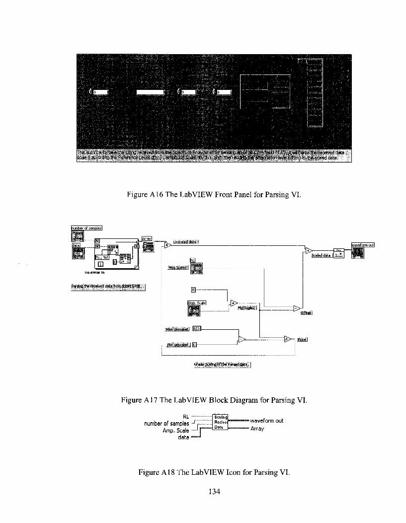
This subVI is to take the strng i»-aved from the Spectrum Analyser after sendbig an SPIB Ccmmand 'TA';, it Sparse the received data , scale >t according the Reference Level(dBm), Amplitude ScaletdB/dM) and then addrg the attenuation level (dBm) to the scaled data

Figure A16 The Lab VIEW Front Panel for Parsing VI.

no error in

Parsing the received data from SubVI GPIB , 0-

lAmp. Scale!

Max Unsealed I I820U

Mln Unstated I |o]

y^ rMSSMEl

y

>. Uavef orm outl

$>i

Scaled data I

^

off ict i

Stopffl

Linear Scaling of {the Parsed data

Figure A17 The Lab VIEW Block Diagram for Parsing VI.

RL number of samples J

r

Amp, 5cale —' | data -~™'

Scaling Rccivc* Data

1 waveform out

• Array

Figure A18 The Lab VIEW Icon for Parsing VI.

134

This SubVI is to send an ASCII Character "C to the senalport of the PC and with certain serial port settngs; waitunt l l l an ASCII character "D" Is received and then end the program,

Figure A19 The Lab VIEW Front Panel for C-D VI.

_J «»IH

0-

|«None T | — '

tsTT^lrrfW HSIrrtr

[Bytes at Port'I

E

Figure A20 The Lab VIEW Block Diagram for C-D VI.

• dup VISA resource name

" read buffer

• Boolean

Figure A21 The Lab VIEW icon for C-D VI.

135

Figure A22 The LabVIEW Front Panel for Senal_com2E VI.

|<>None T

Figure A23 The LabVIEW Block Diagram for Serial_com2E VI.

Figure A24 The LabVIEW Icon for Serial_com2E VI.

136

IThe LabVIEW Program responsible for controlling the moving platform of the Site Survey System and taking measurments from the HP8569B Spectrum analyzer Connected to the PC using the GPIB Card

IFor the Site Survey System Operator see the two parts of the program shown.below; the measurments part and the control part. Input the required values below before running the program.

ummmmmt

B^EKtH '

- 4 0 -

•42 5 J

-45-!

JI7.5-

.80-j

te.5;! -5S-I

57.5-] eo-

•62 'j->

• 0 4 . 3 4 1 5 - ^ ^ ^ ^ ! 7 1 B 2 2.2 2,4 :.o 2.9 3 3 2 3.4 3.6 3.8 • 4.1

I

=-e; 3SSL aw 391 j The Measjf rent Pare cf the Program

,J*nrDtt8tion

I IOO i B H i M ,

Tine Parameters

ymfms-

Notes to The Operator Please specify al the requred inputs nto the cortrol oart-of

the program before wr ing the Program

The Control Part of the Program |

Figure A25 The LabVIEW Front Panel for controlmeasurments VI.

MSC

Figure A26 The LabVIEW Icon for controlmeasurments VI.

137

wm

MM

Mim

mir

imw

nm

iwiw

• a

mi S

tep s

nftg

a pa

stin

g tie

nftf

e aa

tfam

i moto

fs to

step

SEt

atiig

thet

eche

EftJ

W

mea

snre

fe

Figu

re A

27 T

he L

ab V

IEW

blo

ck d

iagr

am f

or c

ontr

olm

easu

rmen

ts.v

i.

138

Appendix B: Moving Platform Program (using Cricket Logo Language)

; Driver program required to use the sensor ports on the expansion board

global [x]

to sensorl

output sens 1

end

to sensor2

output sens 2

end

to sensor3

output sens 3

end

to sensor4

output sens 4

end

to switch 1

output (sens 1) < 128

end

to switch2


end

to switch3


end

to switch4


end

139

to sens :n

bsend$112

setx bsr :n - 1

output x * 256 + bsr 0

end

to counts :n

bsend$112

setx bsr :n + 7


end

to resetc :n

bsend$112

bsend $f + :n ; counter 1 is at $10

bsend 0

end

to velo :n

bsend $112

setx bsr :n + 3


end

to quad12

bsend $112

setx bsr 12


end

toresetql2

bsend $112 bsend $14 bsend 0

end

to quad34

bsend $112

setx bsr 13


end

to resetq34

bsend $112 bsend $15 bsend 0

end

; end of the driver program

; Procedure tracksensor used to make the robot follow the tape

; a program used to make the robot follow the black tape

; motor c is the right motor (s4 sensor is the right sensor)

; motor d is the left motor (si sensor is the left sensor)

;this is to define variables si s4 and choice

global [si s4 choice]

to tracksensor ;procedure tracksensor is the function

; this set the value of the variables , if it this it is true=l , otherwise it is false =0

make the moving platform follow a black tape on ground using left and right

; sensors, if you want to make the robot follow a white tape just change every < 30

; to > 100

sets 1 sensor 1 < 30

sets4 sensor4 < 30

; This is used to identify the si sensors as the most signifcant bit (MSB)

;and the s3 as the least significant bit(LSB) , and replacing them with one parameter

; called "choice"

141

setchoice (si * 2) + s4

; The value of choice (3 Decimal) (11 Binary) means sl=l and s4 =1

; This happens when the si and S4 are in the black tape

; make the power level 2 for both motors

; make them both on for 0.1 second

if choice = 3 [ cd, setpower 2 cd, onfor 1]

;The value of choice (2 decimal) (10 binary ) means sl=l and s4 =0

; in other words s4 is outiside the blacktape and si is inside the black tape

; This happens when the robot is shifted to the right

; it asks the robot to stop the left motor(d) and move the right motor(c) for 0.1 sec

; power level 5 for right motor c

; till it reads all sensors are one

if choice = 2 [ d, off

c, setpower 5 c, onfor 1 ]

; The value of choice (1 decimal) (01 binary ) means sl=0 and s4 =1

; in other words si is outside the black tape and s4 is inside the black tape

; This happens when the robot is shifted to the left

; it asks the robot to stop the right motor(c) and move the left motoifd) for 0.1 sec

; power level 5 for left motor d

; till it reads all sensors are one

if choice = 1 [ c, off d, setpower 5 d, onfor 1]

; this value of the variable zero means the robot is outside the track sl=0 and s4 =0

142

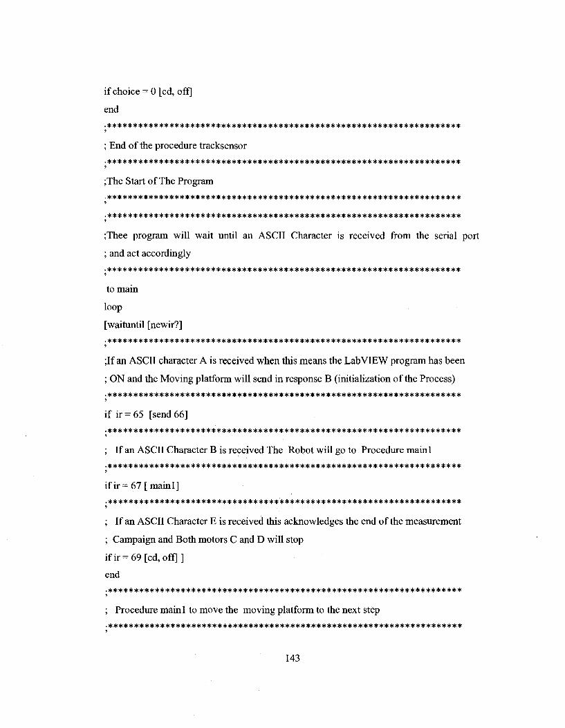
if choice = 0 [cd, off]

end

; End of the procedure tracksensor

;The Start of The Program

;Thee program will wait until an ASCII Character is received from the serial port

; and act accordingly

to main

loop

[waituntil [newir?]

;If an ASCII character A is received when this means the Lab VIEW program has been

; ON and the Moving platform will send in response B (initialization of the Process)

if ir = 65 [send 66]

; If an ASCII Character B is received The Robot will go to Procedure mainl

if ir = 67 [ mainl]

; If an ASCII Character E is received this acknowledges the end of the measurement

; Campaign and Both motors C and D will stop

ifir = 69[cd,off]]

end

; Procedure mainl to move the moving platform to the next step

143

to mainl

cd, setpower 2 ;powerlevel 6 corresponds to voltage = 6xl.5=9v

loop

[ encoder

send 68

stop

]

end

; Procedure Encoder, reads the value of the encoders as the robot is moving

to encoder

; seeing the white sector

if sensora > 180

[ loop [ tracksensor

if sensora < 180 [ stop ] ] ]

; seeing the black sector

if sensora < 180

[ loop [ tracksensor

if sensora > 180 [ stop ] ] ]

stop

144

Appendix C Format of text file generated by the LabVIEW program

This file contains a received power at a distance of 30 cm from the receiver every 2

seconds for period of 58 seconds

Distance(cm) 30.000000 Time (sec) Power (dBm) 0.00000 0.000000

-34.736585 1 2 4 6 8 10

12

14 16 18 20 22

25 26 28

30 32 34 36 38 40 42

44 46 48 50 52 54 56 58

08300 82500 -35 87900 -34 94200 -34 79400 -34 94700

82000

96300 76600 90900 81200 96500

01800 79000 94400 79600

91900 82100

009756 951220 931707 931707

35.029268 35.048780 35.185366 35.146341 34.892683 35.068293 35.068293 34.736585 35.087805 34.834146 35.068293 34.814634 34.834146

97500 -34.756098 76700 -34.853659

-34.912195 -34.814634 -35.263415 -34.392683

98300 -34.931707 77400 -34.970732 89800 -35.048780 98100 -34.951220 76300 -35.048780 92600 -35.185366

92100 98400 75600 9.1900

145

Appendix D: Proof of KG and K24 Having Identical Formulas

This appendix gives a proof to show that the KG formula can be derived from the K24

formula, showing that both are identical. The KG formula is (3.5)

_ (2fi2 -MA) m n

Mi~V-Mi -Mt)

Multiplying the numerator and denominator of the (D.l) by /J2 + y./ul - juA) and

rearranging them results in

KG = 2Ml-MA+Ml(2Ml-M<Y (D 2)

MA-Mi

To make (D.2) identical to the K24 formula, we multiply the numerator and the

denominator of (D.2) by -1 this gives

KG = -1M22+M<-M2(2M2

2-MT t ( D 3 )

Mi ~MA

This is the formula for K24 given by (3.13)

146

Appendix E: Path Loss Index Derivation

The square error is given by

m

Q = YJ{VdBi-Ko-n20\ozri))2 . (E.l)

;=1

To find the values for VdB0 and n that make Q minimized, taking the partial derivative

of Q with respect to VdB0 and set it equal to zero and taking the partial derivative of Q

with respect to n and set it equal to zero results in

dQ = 2fj(VdBi-VdB0+n20logr,.)i-l) = 0 (E.2) rffiO i"=l

^- = 2ZK, -V*B» +/i201ogr,X201og/;.) = 0. (E.3) on ~T

Arranging (E2) results in

S ( ^ o - ^ - « 2 0 1 o g r , ) = 0. (E.4)

147

Expressing VdB0 in terms of other quantities results in

V - — r <mo

Z^,+"Z201ogr, 1=1 /=i

m (E.5)

Arranging (E3) results in

£ ^ , 2 0 1 o g ^ . - ^ 0 £ 2 0 1 o g r , . +W£(201og/;.)2 = 0 . (E.6)

Substituting (E.5) in (E.6) and arranging to find n in terms of other quantities results in

m m

I^,l201ogy-mX^,201og(,; .) 1=1 1=1 ;=1

m| ; (201og( n ) ) 2 - |]201og(r,.)

(E.7)

148

rician-k factor study for temporal and spatial variations · 395 wellington street ottawa on k1a0n4...

Documents