richard a. davis and gabriel rodriguez-yam …rdavis/lectures/unsw_03.pdf · 1 estimation for state...
TRANSCRIPT
1
Estimation for State Space Models: Estimation for State Space Models: an Approximate Likelihood Approachan Approximate Likelihood Approach
Richard A. Davis and Gabriel Rodriguez-YamColorado State University
(http://www.stat.colostate.edu/~rdavis/lectures)
Joint work with:William Dunsmuir, University of New South WalesYing Wang, Dept of Public Health, W. Virginia

2
Example: Daily Asthma Presentations (1990:1993)
Year 1990
••••••••••
•••••
•••••••••••••••••
•••••
•
••••••
••••••••••••
••••
•••••••••••
••••••••
•••••••••
•••
••
••••
••••••
•••••
••
•
•••••••••••••••••••••
••
•
•••••
•
••••
•••••••
••••
•
••••••••••••
•
••••••
•••••
•
•••
•
••••••
•••••••••
•
•••••••
•
•••••••••••••
••••••••••
••••••••••
••••••••••••
••••••
•••••
••••••••
••••••••••••
•••••••
•••••••••••
••••••••••••
•
•••••••••••••
•••••
••••••••••••
••••••••
••••••
••••
06
14
Jan Feb Mar Apr May Jun Jul Aug Sep Oct Nov Dec
Year 1991
••••••
••••••••••••
•••••••••
••••••••
•••••
••
•••••
••••••
••••••
••••••
•••••••••
••
•••
••••••
•
•••••••
•
••••••
••••••••
••••••••••••••
•••••
•••••
•
•
•
•••
•••••••••
••••••••
••••••••
••••••••••••
•
•••••••
••••
••••••
•••••••••••
•••••
•••••••
•
••••••••••••
••••
••••••••••
•••••••••••••••••••••••••••
••••••••
•••••
•••••
••••••••••
•••••••
•••••••••••••
•••••
••••••••••
•••••••••••••
••••••••••
•••••••••
06
14
Jan Feb Mar Apr May Jun Jul Aug Sep Oct Nov Dec
Year 1992
•
•••••••••
••••••••••••••••••••
••••••••
•
••••••••••
••
•••••
••
••
••••••••••
••
•
••
•••••
•••••
••••••
•••••••
•••
••••
••••••••••
•••
•••••••••
•••••••••
••••••
••
•
••
•
•
••
•
•••••••
•
•••••••
••••
•
•••••
••••••
•••••••••
••••••••••••
••••••
•••••••••
••••
••••••••
•••
••••••••
••••••••
•••••••••••••
•••••
••••••
••••••••••
••••••••
•••••••
•••••••••
•••••••••
•
•••••••
•
••••••••
••••••••••••
••••••••
•••••
•••••••0
614
Jan Feb Mar Apr May Jun Jul Aug Sep Oct Nov Dec
Year 1993
••••••••••••
••••••••
•••••
•••••
•••••••••••
•••
••••
••
••••
••••
•
•
•••••••
•
•••••••••••
••
•••••••••
••••
••
••
••••••••
•••••••••
••••••••
•••••••••••
•
•••••••••••
••••
••••••
••
••••••
••
•••••
•••••••••••
•••••••••
•••••••
••••
••••••••••••
•••••••
•••••
••••••••
••••••
•••••••
•••••
•••••••
•••••
•••••
•••••
•••••••••
•
••••••••••••••••••••
••••
••••
•••••••
•••••••••••••••••••••
••••
•••••••••
••••••••••••0
614
Jan Feb Mar Apr May Jun Jul Aug Sep Oct Nov Dec

3
day
log
retu
rns
(exc
hang
e ra
tes)
0 200 400 600 800
-20
24
lag
AC
F
0 10 20 30 40
0.0
0.2
0.4
0.6
0.8
1.0
lag
AC
F of
squ
ares
0 10 20 30 40
0.0
0.2
0.4
0.6
0.8
1.0
lag
AC
F of
abs
val
ues
0 10 20 30 40
0.0
0.2
0.4
0.6
0.8
1.0
Example: Pound-Dollar Exchange Rates (Oct 1, 1981 - June28, 1985; Koopman website)
4
Motivating Examples• Time series of counts• Stochastic volatility
Generalized state-space modelsObservation drivenParameter driven
Model setup and estimationGeneralized linear models (GLM)Estimating equations (Zeger)MCEM (Chan and Ledolter)Importance sampling
- Durbin and KoopmanApproximation to the likelihood (Davis, Dunsmuir, and Wang)
ApplicationTime series of countsStochastic volatility
5
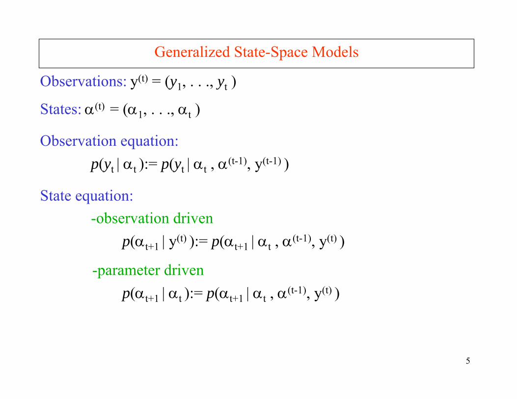
Generalized State-Space Models
Observations: y(t) = (y1, . . ., yt )
States: α(t) = (α1, . . ., αt )
Observation equation:p(yt | αt ):= p(yt | αt , α(t-1), y(t-1) )
State equation:-observation driven
p(αt+1 | y(t) ):= p(αt+1 | αt , α(t-1), y(t) )
-parameter drivenp(αt+1 | αt ):= p(αt+1 | αt , α(t-1), y(t) )
6
..., 1, ,0 ,!
e)|( tt
e
tt
ttt
==αα−−α
yy
ypy
..., 1, ,0 ,!
e)|( tt
e
tt
ttt
==αα−−α
yy
ypy
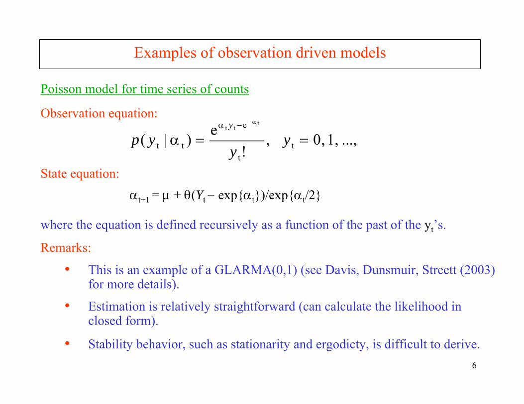
Examples of observation driven models
Poisson model for time series of counts
Observation equation:
State equation:αt+1 = µ + θ(Yt − expαt)/expαt/2
where the equation is defined recursively as a function of the past of the yt’s.
whereRemarks:
• This is an example of a GLARMA(0,1) (see Davis, Dunsmuir, Streett (2003) for more details).
• Estimation is relatively straightforward (can calculate the likelihood in closed form).
• Stability behavior, such as stationarity and ergodicty, is difficult to derive.

7
Examples of observation driven models-cont
An observation driven model for financial data:Model (GARCH(p,q)):
Yt = σt Zt , Zt~IID N(0,1)
Special case (ARCH(1)=GARCH(1,0)): The resulting observation and state transition density/equations are
p(yt| σt) = n(yt ; 0, σ2t )
2211
22110
2qtqtptptt YY −−−− σβ++σβ+α++α+α=σ LL
2110
2−α+α=σ tt Y
Properties:
• Martingale difference sequence.
• Stationary for α1 ∈[0,2eE), E-Euler’s constant.
• Strongly mixing at a geometric rate.
• For general ARCH (GARCH), properties are difficult to establish.
8
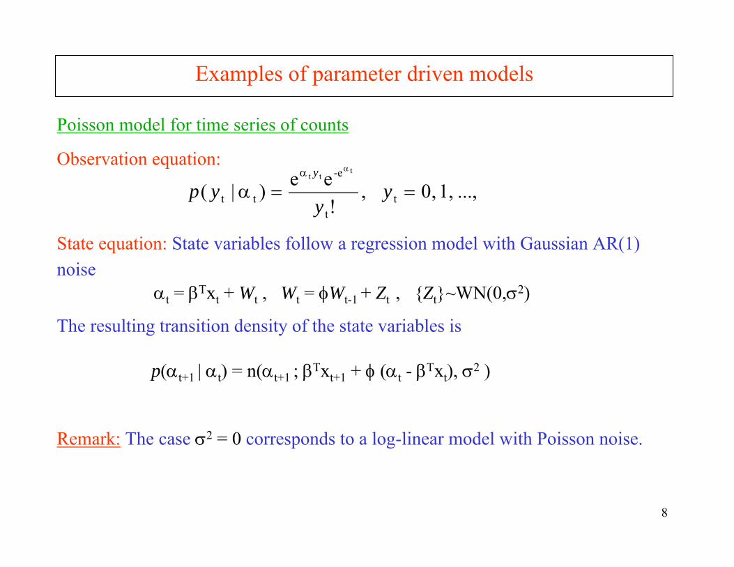
Examples of parameter driven models
Poisson model for time series of counts
Observation equation:
..., 1, ,0 ,!
ee)|( tt
-e
tt
ttt
==ααα
yy
ypy
Remark: The case σ2 = 0 corresponds to a log-linear model with Poisson noise.
State equation: State variables follow a regression model with Gaussian AR(1) noise AR(1) noise:
αt = βΤxt + Wt , Wt = φWt-1 + Zt , Zt~WN(0,σ2)
The resulting transition density of the state variables is
is p(αt+1 | αt) = n(αt+1 ; βΤxt+1 + φ (αt - βΤxt), σ2 )
9
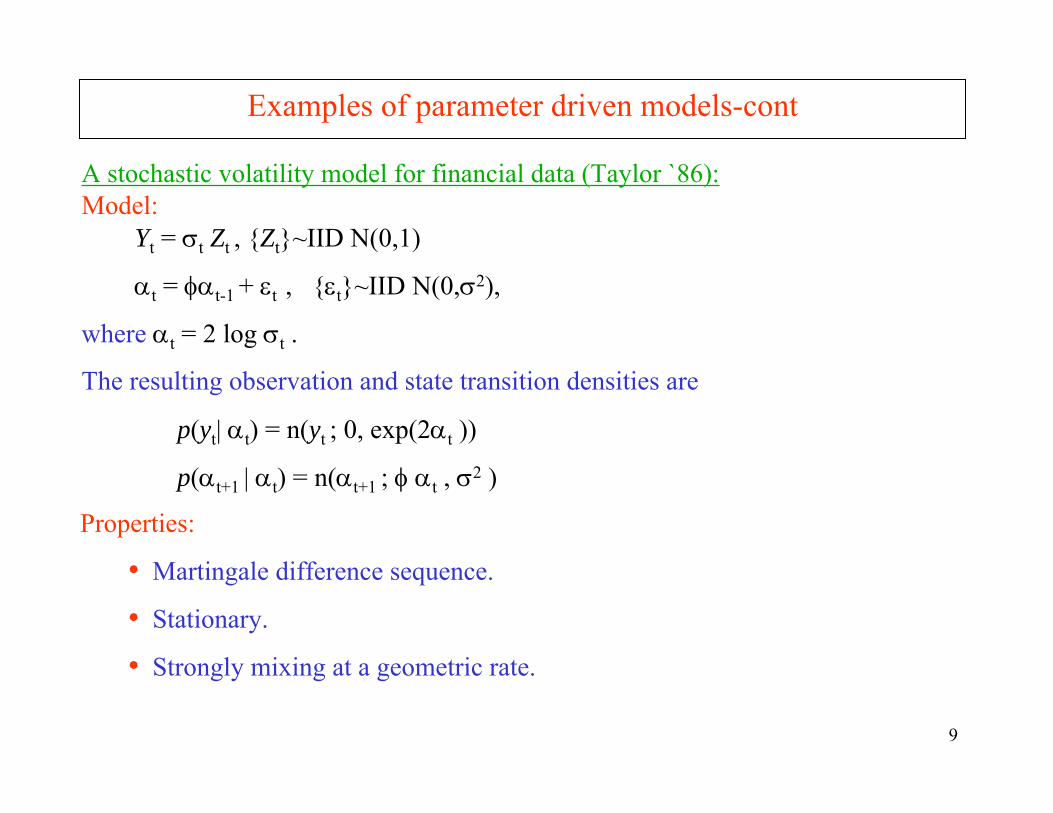
Examples of parameter driven models-cont
A stochastic volatility model for financial data (Taylor `86):Model:
Yt = σt Zt , Zt~IID N(0,1)
αt = φαt-1 + εt , εt~IID N(0,σ2),
where αt = 2 log σt .
The resulting observation and state transition densities are
p(yt| αt) = n(yt ; 0, exp(2αt ))
p(αt+1 | αt) = n(αt+1 ; φ αt , σ2 )
Properties:
• Martingale difference sequence.
• Stationary.
• Strongly mixing at a geometric rate.
10
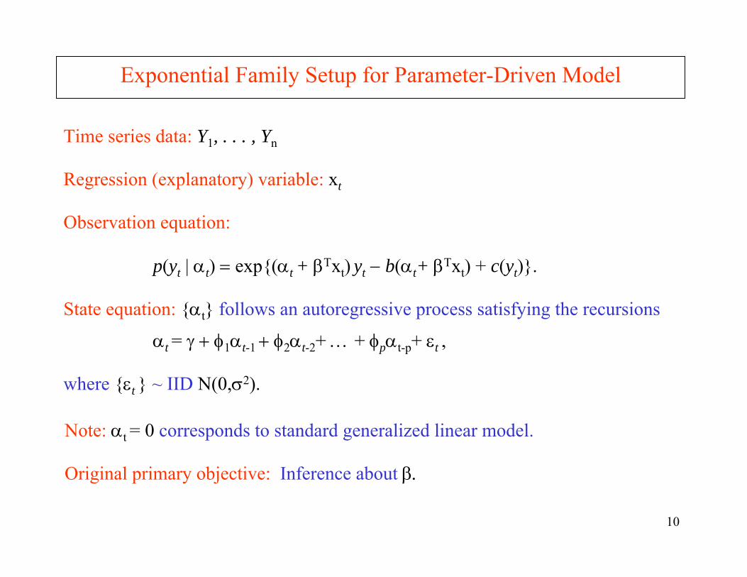
Exponential Family Setup for Parameter-Driven Model
Time series data: Y1, . . . , Yn
Regression (explanatory) variable: xt
Observation equation:
p(yt | αt) = exp(αt + βΤxt) yt − b(αt+ βΤxt) + c(yt).
State equation: αt follows an autoregressive process satisfying the recursions
αt = γ + φ1αt-1 + φ2αt-2+ … + φpαt-p+ εt ,
where εt ~ IID N(0,σ2).
Note: αt = 0 corresponds to standard generalized linear model.
Original primary objective: Inference about β.
11
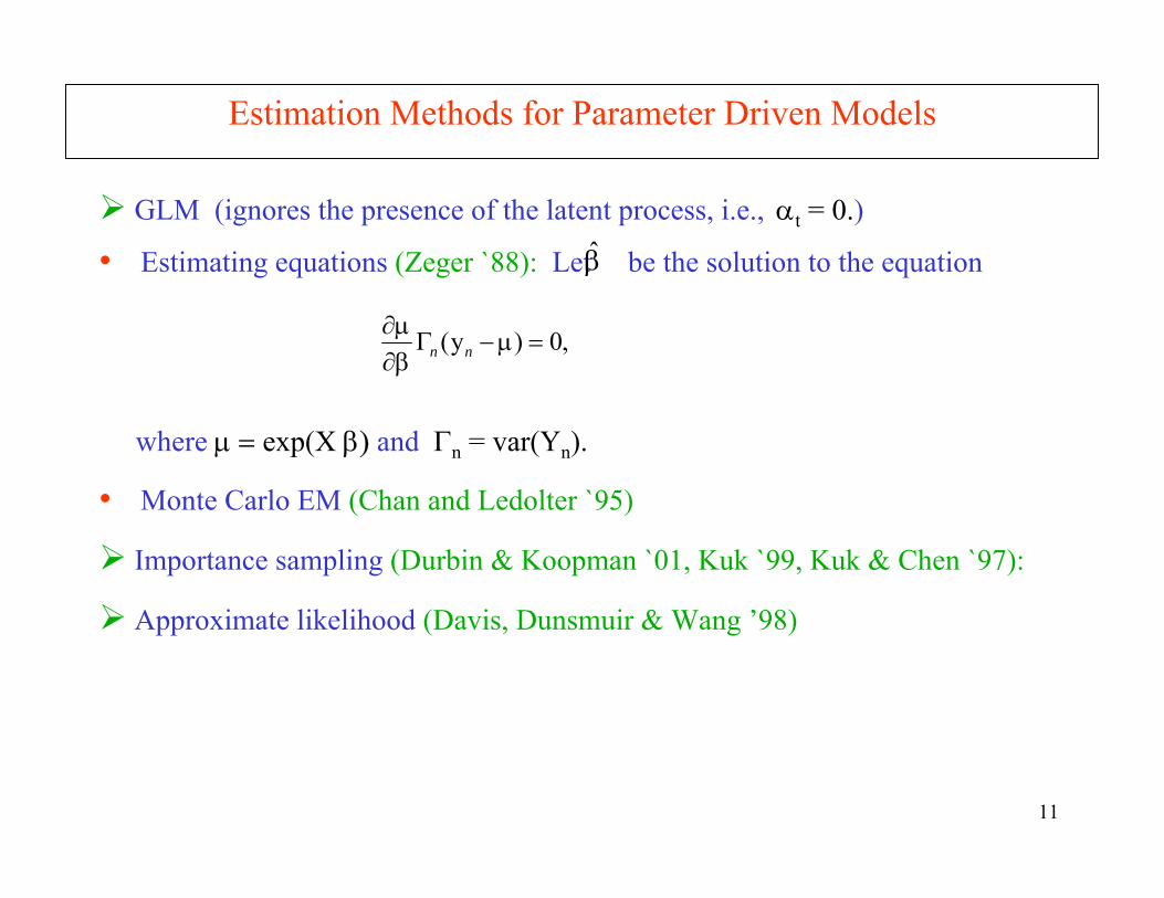
GLM (ignores the presence of the latent process, i.e., αt = 0.)
• Estimating equations (Zeger `88): Let be the solution to the equation
where µ = exp(X β) and Γn = var(Yn).
• Monte Carlo EM (Chan and Ledolter `95)
Importance sampling (Durbin & Koopman `01, Kuk `99, Kuk & Chen `97):
Approximate likelihood (Davis, Dunsmuir & Wang ’98)
Estimation Methods for Parameter Driven Models
,0)y( =µ−Γβ∂µ∂
nn
β
12
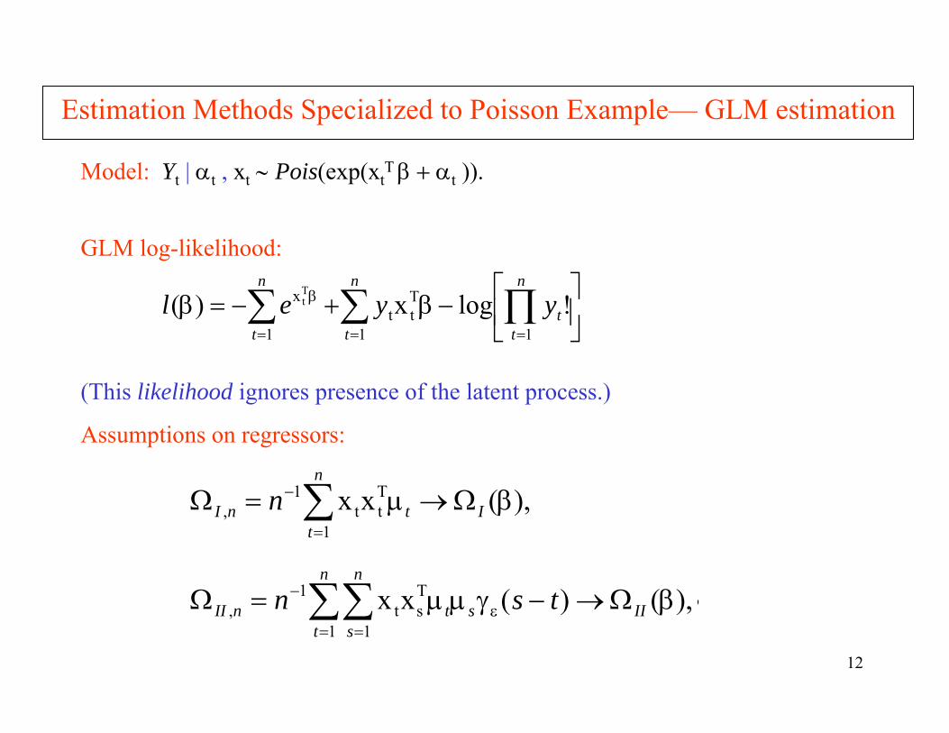
Model: Yt | αt , xt ∼ Pois(exp(xtT β + αt )).
GLM log-likelihood:
(This likelihood ignores presence of the latent process.)
⎥⎦
⎤⎢⎣
⎡−β+−=)β ∏∑∑===
βn
tt
n
t
n
t
yyel11
Ttt
1
x !logx(Tt
Estimation Methods Specialized to Poisson Example— GLM estimation
Assumptions on regressors:
),()(xx
),(xx
1 1
Tst
1,
1
Ttt
1,
βΩ→−γµµ=Ω
βΩ→µ=Ω
∑∑
∑
=ε
=
−
=
−
II
n
ts
n
stnII
I
n
ttnI
tsn
n
),()(xx
),(xx
1 1
Tst
1,
1
Ttt
1,
βΩ→−γµµ=Ω
βΩ→µ=Ω
∑∑
∑
=ε
=
−
=
−
II
n
ts
n
stnII
I
n
ttnI
tsn
n

13
Theorem (Davis, Dunsmuir, Wang `00). Let be the GLM estimate of βobtained by maximizing l(β) for the Poisson regression model with a stationary lognormal latent process. Then
). N(0, )βˆ( 1III
1I
1I
2/1 −−− ΩΩΩ+Ω→−βd
n
Theory of GLM Estimation in Presence of Latent Process
Notes:
1. n-1ΩI-1 is the asymptotic cov matrix from a std GLM analysis.
2. n-1ΩI-1 ΩII ΩI
-1 is the additional contribution due to the presence of the latentprocess.
3. Result also valid for more general latent processes (mixing, etc),
4. The xt can depend on the sample size n.
β

14
Assume the αt follows a log-normal AR(1), where
(αt+σ2/2) = φ(αt-1+ σ2/2) +ηt , ηt~IID N(0, σ2(1−φ2)),
with φ =.82, σ2 = .57.
βZ s.e. βGLM s.e. s.e. βGLM s.d.
Application to Model for Polio Data
Zeger GLM Fit Asym Simulation
Intercept 0.17 0.17 0.13Trend(×10-3) -4.35 2.68cos(2πt/12) -0.11 0.16sin(2πt/12) -.048 0.17cos(2πt/6) 0.20 0.14sin(2πt/6) -0.41 0.14
.207 .075 .205-4.80 1.40 4.12-0.15 .097 .157-0.53 .109 .168.169 .098 .122-.432 .101 .125
.150 .213-4.89 3.94-.145 .144-.531 .168.167 .123-.440 .125
15
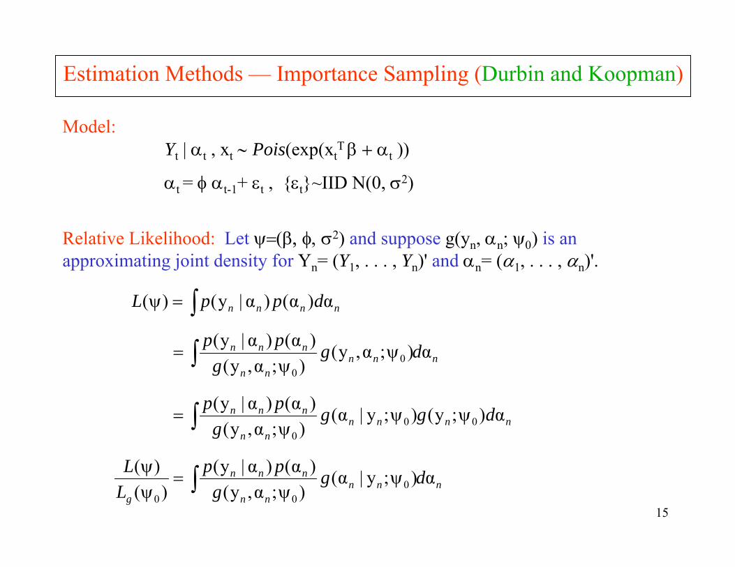
Estimation Methods — Importance Sampling (Durbin and Koopman)
Model: Yt | αt , xt ∼ Pois(exp(xt
T β + αt ))
αt = φ αt-1+ εt , εt~IID N(0, σ2)
Relative Likelihood: Let ψ=(β, φ, σ2) and suppose g(yn, αn; ψ0) is an approximating joint density for Yn= (Y1, . . . , Yn)' and αn= (α1, . . . , αn)'.
nnnn dppL α)α()α|y()( ∫=ψ
nnnnn
nnn
g
nnnnnn
nnn
nnnnn
nnn
dgg
ppLL
dggg
pp
dgg
pp
α);y|α();α,y(
)α()α|y()(
)(
α);y();y|α();α,y(
)α()α|y(
α);α,y();α,y(
)α()α|y(
000
000
00
∫
∫
∫
ψψ
=ψψ
ψψψ
=
ψψ
=
nnnnn
nnn
g
nnnnnn
nnn
nnnnn
nnn
dgg
ppLL
dggg
pp
dgg
pp
α);y|α();α,y(
)α()α|y()(
)(
α);y();y|α();α,y(
)α()α|y(
α);α,y();α,y(
)α()α|y(
000
000
00
∫
∫
∫
ψψ
=ψψ
ψψψ
=
ψψ
=

16
Importance Sampling (cont)
where
,);α,y(
)α()α|y(1~
);y|);α,y(
)α()α|y(
α);y|α();α,y(
)α()α|y()(
)(
1 0)(
)()(
00
000
∑
∫
= ψ
⎥⎦
⎤⎢⎣
⎡ψ
ψ=
ψψ
=ψψ
N
jj
nn
jn
jnn
nnn
nnng
nnnnn
nnn
g
gpp
N
gppE
dgg
ppLL
).;y|g(α iid ~,...,1;α 0)( ψ= nn
jn Nj
.ψ
Notes:
• This is a “one-sample” approximation to the relative likelihood. That is, for one realization of the α’s, we have, in principle, an approximation to the whole likelihood function.
• Approximation is only good in a neighborhood of ψ0. Geyer suggests maximizing ratio wrt ψ and iterate replacing ψ0 with

17phi
log
likel
ihoo
d
0.3 0.4 0.5 0.6 0.7
-416
-415
-414
-413
-412
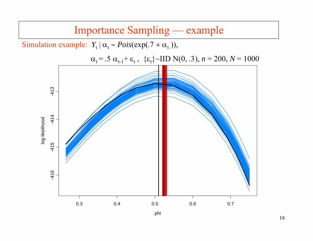
Importance Sampling — exampleSimulation example: Yt | αt ∼ Pois(exp(.7 + αt )),
αt = .5 αt-1+ εt , εt~IID N(0, .3), n = 200, N = 1000
18phi
log
likel
ihoo
d
0.3 0.4 0.5 0.6 0.7
-416
-415
-414
-413
Simulation example: Yt | αt ∼ Pois(exp(.7 + αt )),
αt = .5 αt-1+ εt , εt~IID N(0, .3), n = 200, N = 1000
Importance Sampling — example
19
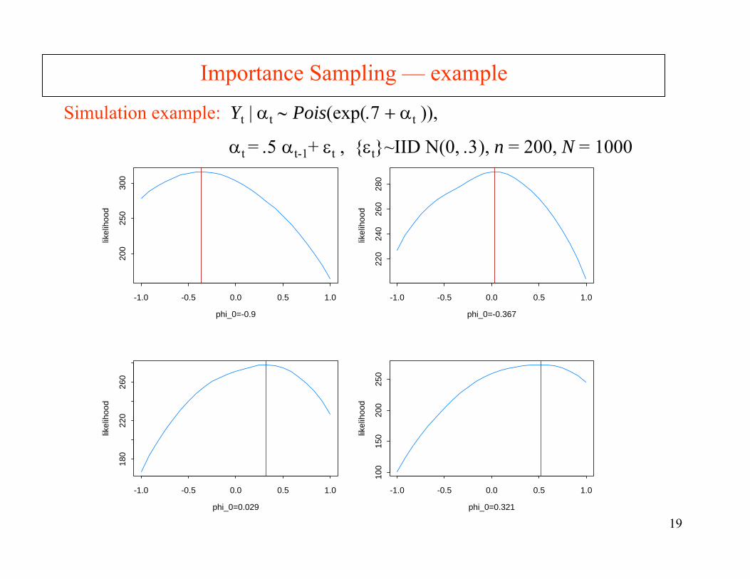
Importance Sampling — example
phi_0=-0.9
likel
ihoo
d
-1.0 -0.5 0.0 0.5 1.0
200
250
300
phi_0=-0.367
likel
ihoo
d
-1.0 -0.5 0.0 0.5 1.0
220
240
260
280
phi_0=0.029
likel
ihoo
d
-1.0 -0.5 0.0 0.5 1.0
180
220
260
phi_0=0.321
likel
ihoo
d
-1.0 -0.5 0.0 0.5 1.0
100
150
200
250
Simulation example: Yt | αt ∼ Pois(exp(.7 + αt )),
αt = .5 αt-1+ εt , εt~IID N(0, .3), n = 200, N = 1000

22
Importance Sampling (cont)
Choice of importance density g:
Durbin and Koopman suggest a linear state-space approximating model
Yt = µt+ xtT β + αt+Zt , Zt~N(0,Ht),
with
where the are calculated recursively under the approximating model until convergence.
),,y~(~);y|g(α 110
−− ΓΓψ nnnnn N
.))'αα(()(diag
,αyy~ 1αXβ
αXβαXβ n
−+
++
+=Γ
+−=
nnn
nnn
Ee
een
n
With this choice of approximating model, it turns out that
where
)y|(ˆ ntgt E α=α,
,1'xˆ
)'xˆ(
)'xˆ(t
β+α−
β+α−
=
+−α−=µ
tt
tt
eH
eyy
t
tttt
,
,1'xˆ
)'xˆ(
)'xˆ(t
β+α−
β+α−
=
+−α−=µ
tt
tt
eH
eyy
t
tttt
23
Importance Sampling (cont)
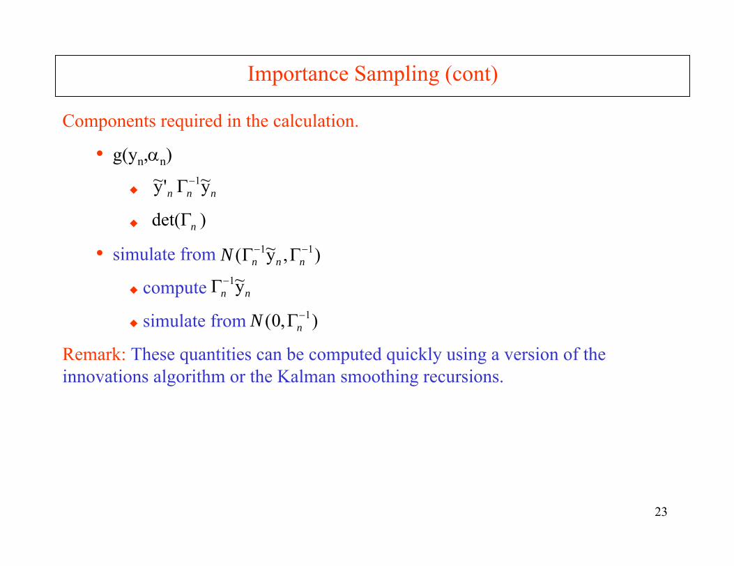
Components required in the calculation.
• g(yn,αn)
• simulate from
compute
simulate from
Remark: These quantities can be computed quickly using a version of the innovations algorithm or the Kalman smoothing recursions.
nnn y~'y~ 1−Γ
)det( nΓ
),y~( 11 −− ΓΓ nnnN
nn y~1−Γ
),0( 1−ΓnN

24
Importance Sampling — example
Simulation example: β = .7, φ = .5, σ2=.3, n = 200, N = 1000, 50 realizations plotted
phi_0=-0.5
likel
ihoo
d
-1.0 -0.5 0.0 0.5 1.0
180
220
260
300
phi_0=-0.25
likel
ihoo
d-1.0 -0.5 0.0 0.5 1.0
200
220
240
260
280
phi_0=0
likel
ihoo
d
-1.0 -0.5 0.0 0.5 1.0
160
180
200
220
240
260
280
phi_0=0.25
likel
ihoo
d
-1.0 -0.5 0.0 0.5 1.0
150
200
250
phi_0=0.5
likel
ihoo
d
-1.0 -0.5 0.0 0.5 1.0
5010
015
020
025
0
phi_0=0.75
likel
ihoo
d
-1.0 -0.5 0.0 0.5 1.050
100
150
200
250
26
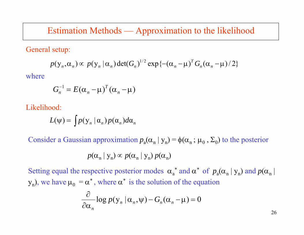
Consider a Gaussian approximation pa(αn | yn) = φ(αn ; µ0 , Σ0) to the posterior
p(αn | yn) ∝ p(αn | yn) p(αn)
Setting equal the respective posterior modes αa* and α* of pa(αn | yn) and p(αn |
yn), we have µ0 = α* , where α* is the solution of the equation
Estimation Methods — Approximation to the likelihood
General setup:
where
Likelihood:
2/)()(exp)det()|y(),y( 2/1 µ−αµ−α−α∝α nnT
nnnnnn GGpp 2/)()(exp)det()|y(),y( 2/1 µ−αµ−α−α∝α nnT
nnnnnn GGpp
)()(1 µ−αµ−α=−n
Tnn EG )()(1 µ−αµ−α=−
nT
nn EG
nnnn dppL α)α()α|y()( ∫=ψ nnnn dppL α)α()α|y()( ∫=ψ
0)(),|y(log =µ−α−ψαα∂∂
nnnnn
Gp 0)(),|y(log =µ−α−ψαα∂∂
nnnnn
Gp
27
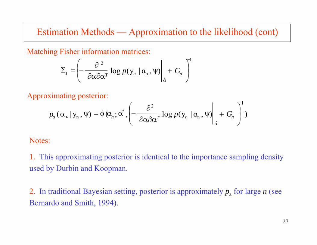
Notes:
1. This approximating posterior is identical to the importance sampling density used by Durbin and Koopman.
Estimation Methods — Approximation to the likelihood (cont)
Matching Fisher information matrices:
Approximating posterior:
2. In traditional Bayesian setting, posterior is approximately pa for large n (see Bernardo and Smith, 1994).
1
n
2
0*
),α|y(log−
α⎟⎟⎠
⎞⎜⎜⎝
⎛+ψ
α∂α∂∂
−=Σ nnTGp
)),α|y(log,;(),y|(1
n
2*
n*
−
α⎟⎟⎠
⎞⎜⎜⎝
⎛+ψ
α∂α∂∂
−ααφ=ψα nnTnna Gpp
28
2/1
n
2
***n
2/1
n***
nn
*
),α|y(logdet
2/)()(exp),|y(||
),y|(/),(),|y()y;(
⎟⎟⎠
⎞⎜⎜⎝
⎛+ψ
α∂α∂∂−
µ−αµ−α−ψα=
ψαψαψα=ψ
αnnT
nT
n
aa
Gp
GpG
pppL
Estimation Methods — Approximation to the likelihood (cont)
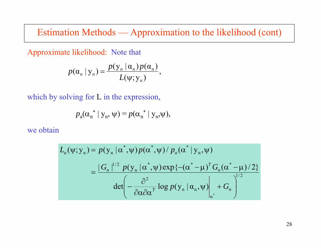
Approximate likelihood: Note that
which by solving for L in the expression,
pa(αn* | yn, ψ) = p(αn
* | yn,ψ),
,)y;(
)α()α|y()y|(α n
nnnnn L
pppψ
=
we obtain
,)y;(
)α()α|y()y|(α n
nnnnn L
pppψ
=
2/1
n
2
***n
2/1
n***
nn
*
),α|y(logdet
2/)()(exp),|y(||
),y|(/),(),|y()y;(
⎟⎟⎠
⎞⎜⎜⎝
⎛+ψ
α∂α∂∂−
µ−αµ−α−ψα=
ψαψαψα=ψ
αnnT
nT
n
aa
Gp
GpG
pppL
29
Estimation Methods — Approximation to the likelihood (cont)
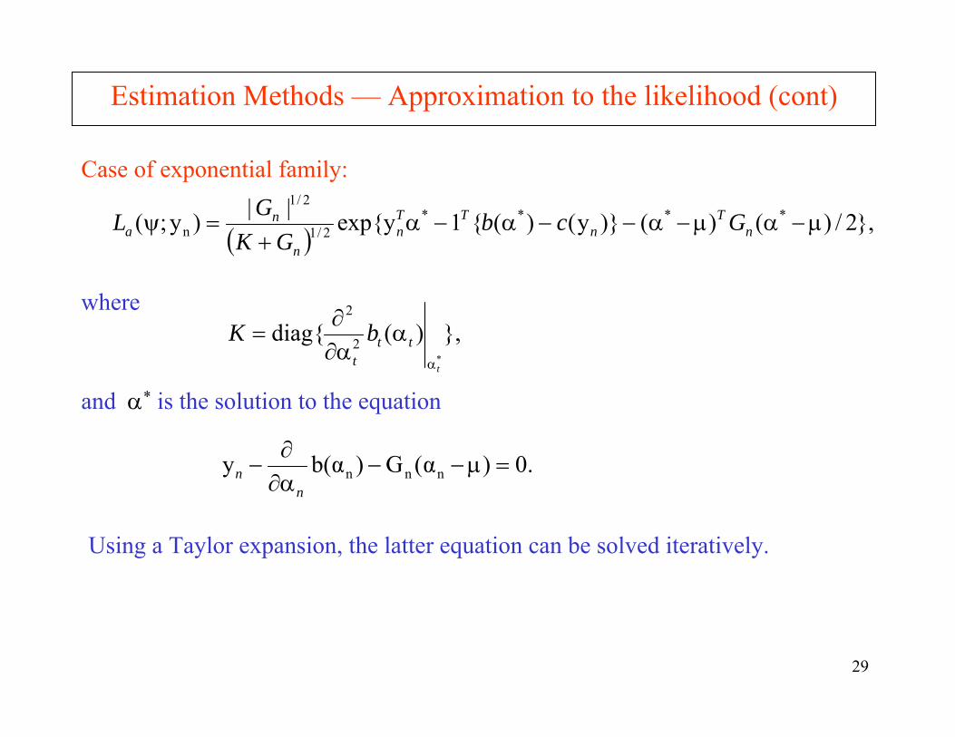
Case of exponential family:
where
and α* is the solution to the equation
( ),2/)()()y()(1yexp||)y;( ****
2/1
2/1
n µ−αµ−α−−α−α+
=ψ nT
nTT
nn
na Gcb
GKGL
,)(diag*
2
2
t
ttt
bKα
αα∂∂
=
.0)α(G)b(αy nnn =µ−−α∂∂
−n
n
Using a Taylor expansion, the latter equation can be solved iteratively.

30
Estimation Methods — Approximation to the likelihood
Implementation:
1. Let α∗= α∗(ψ) be the converged value of α(j) (ψ) , where
and
2. Maximize with respect to ψ.
),(y~)b()(α jn
-1j)1( ψ+=ψ+n
j G&&
);y( ψnap
.Gαbbyy~ n(j)jj
njn µ++−= &&&
31
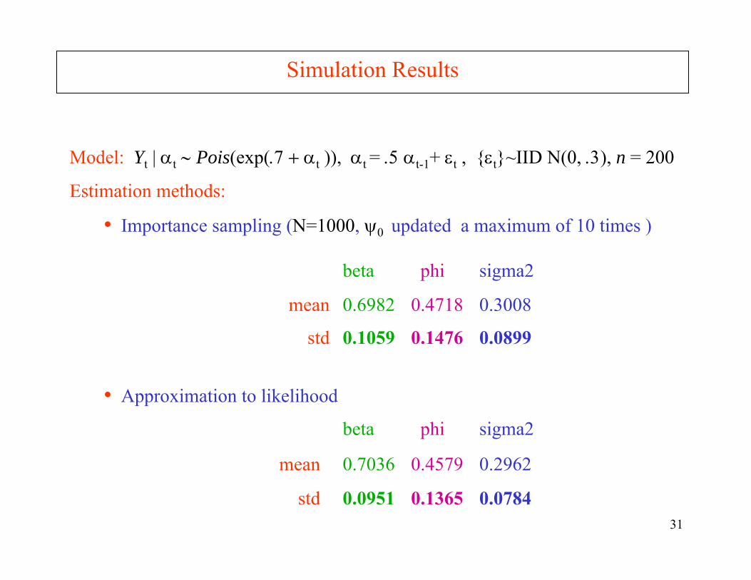
Model: Yt | αt ∼ Pois(exp(.7 + αt )), αt = .5 αt-1+ εt , εt~IID N(0, .3), n = 200
Estimation methods:
• Importance sampling (N=1000, ψ0 updated a maximum of 10 times )
beta phi sigma2
mean 0.6982 0.4718 0.3008
std 0.1059 0.1476 0.0899
Simulation Results
• Approximation to likelihood
beta phi sigma2
mean 0.7036 0.4579 0.2962
std 0.0951 0.1365 0.0784
32
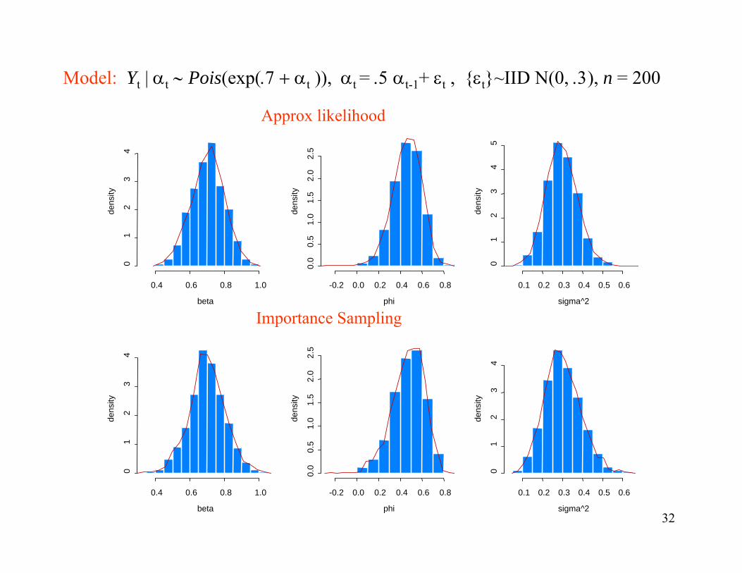
Model: Yt | αt ∼ Pois(exp(.7 + αt )), αt = .5 αt-1+ εt , εt~IID N(0, .3), n = 200
0.4 0.6 0.8 1.0
01
23
4
beta
dens
ity
-0.2 0.0 0.2 0.4 0.6 0.8
0.0
0.5
1.0
1.5
2.0
2.5
phide
nsity
0.1 0.2 0.3 0.4 0.5 0.6
01
23
45
sigma^2
dens
ity
Approx likelihood
0.4 0.6 0.8 1.0
01
23
4
beta
dens
ity
-0.2 0.0 0.2 0.4 0.6 0.8
0.0
0.5
1.0
1.5
2.0
2.5
phi
dens
ity
0.1 0.2 0.3 0.4 0.5 0.60
12
34
sigma^2
dens
ity
Importance Sampling

33
Approx Like Simulation
0.202 0.210 0.343 -2.690 -2.720 3.4150.113 0.111 0.123-0.454 -0.454 0.1430.396 0.400 0.1140.016 0.012 0.1100.845 0.764 0.1650.104 0.114 0.075
ISˆ β Mean SD
Model for αt:αt = φαt-1+εt , εt~IID N(0, σ2).
• Importance sampling ( ψ0 updated 5 times for each N=100, 500, 1000, )• Simulation based on 1000 replications and the fitted AL model.
Application to Model Fitting for the Polio Data
Import Sampling Simulation
Intercept 0.203 0.223 0.381Trend(×10-3) -2.675 -2.778 3.979cos(2πt/12) 0.110 0.103 0.124sin(2πt/12) -0.456 -0.456 0.151cos(2πt/6) 0.399 0.401 0.123sin(2πt/6) 0.015 0.024 0.118 φ 0.865 0.777 0.198 σ2 0.088 0.100 0.068
ALˆ β Mean SD GLM
ˆ β SD
GLM
.207 0.078-4.18 1.400-.152 0.097-.532 0.109.169 0.098-.432 0.101
34
-15 -10 -5 0 5
0.0
0.04
0.08
0.12
beta1
dens
ity
-0.2 0.2 0.4 0.6 0.8 1.00
12
34
phi
dens
ity
0.0 0.1 0.2 0.3 0.4
02
46
sigma^2
dens
ity
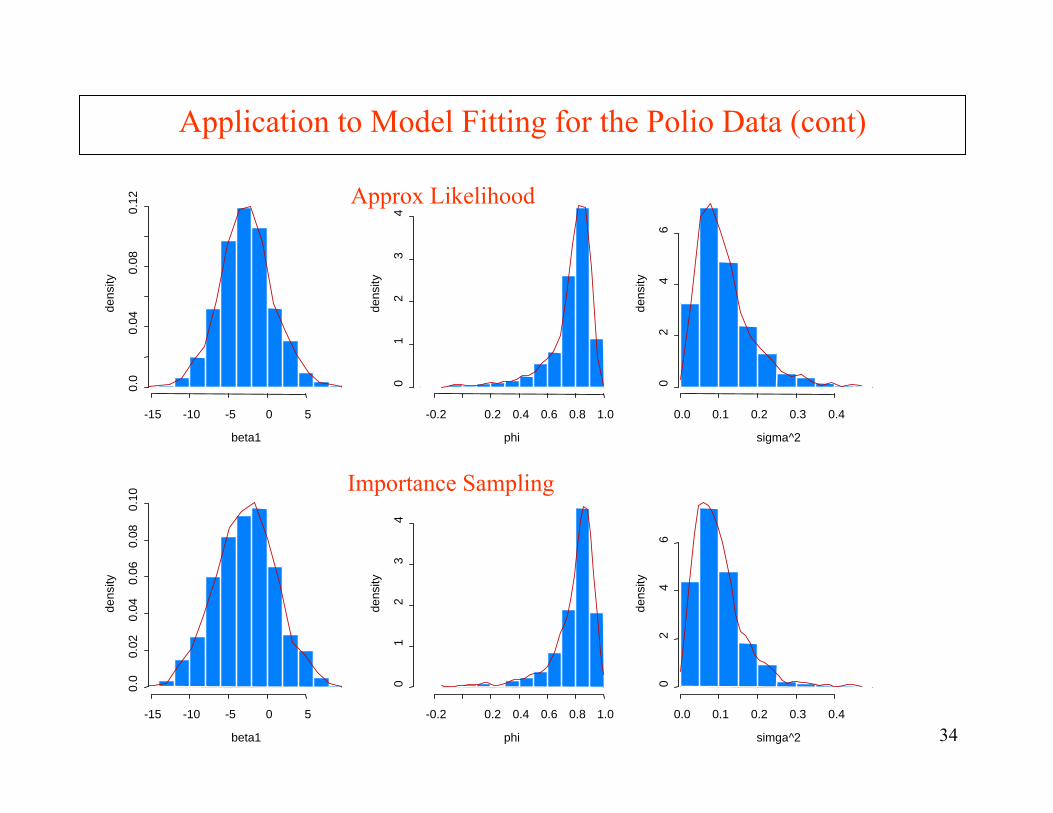
Application to Model Fitting for the Polio Data (cont)
Approx Likelihood
-15 -10 -5 0 5
0.0
0.02
0.04
0.06
0.08
0.10
beta1
dens
ity
-0.2 0.2 0.4 0.6 0.8 1.0
01
23
4
phi
dens
ity
0.0 0.1 0.2 0.3 0.4
02
46
simga^2
dens
ity
Importance Sampling

35
Simulation Results
Stochastic volatility model:Yt = σt Zt , Zt~IID N(0,1)
αt = γ + φαt-1 + εt , εt~IID N(0,σ2), where αt = 2 log σt ; n=1000, NR=500
RMSE RMSE
.210 .216
.025 .026
.065 .073
True AL
γ −.411 −.491
φ 0.950 0.940
σ 0.484 0.478
IS
−.490
0.940
0.481
RMSE RMSE
.341 .324
.046 .043
.068 .068
True AL
γ −.368 −.499
φ 0.950 0.932
σ 0.260 0.270
IS
−.485
0.934
0.268
CV=10
CV=1
36
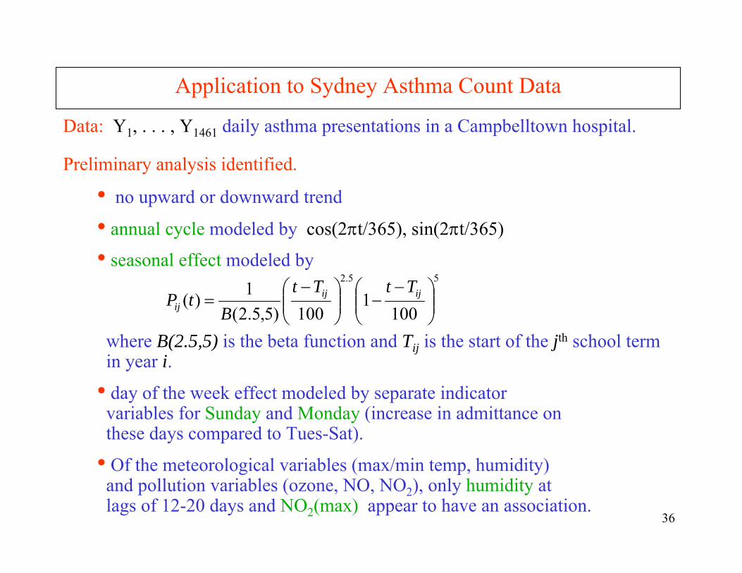
Application to Sydney Asthma Count Data
Data: Y1, . . . , Y1461 daily asthma presentations in a Campbelltown hospital.
Preliminary analysis identified.
• no upward or downward trend
• annual cycle modeled by cos(2πt/365), sin(2πt/365)
• seasonal effect modeled by
where B(2.5,5) is the beta function and Tij is the start of the jth school term in year i.
• day of the week effect modeled by separate indicatorvariables for Sunday and Monday (increase in admittance on these days compared to Tues-Sat).
• Of the meteorological variables (max/min temp, humidity)and pollution variables (ozone, NO, NO2), only humidity at lags of 12-20 days and NO2(max) appear to have an association.
55.2
1001
100)5,5.2(1)( ⎟⎟
⎠
⎞⎜⎜⎝
⎛ −−⎟⎟
⎠
⎞⎜⎜⎝
⎛ −= ijij
ij
TtTtB
tP
37
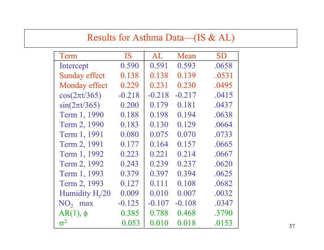
Results for Asthma Data—(IS & AL)
Term IS Intercept 0.590Sunday effect 0.138Monday effect 0.229cos(2πt/365) -0.218 sin(2πt/365) 0.200Term 1, 1990 0.188Term 2, 1990 0.183Term 1, 1991 0.080Term 2, 1991 0.177Term 1, 1992 0.223Term 2, 1992 0.243Term 1, 1993 0.379Term 2, 1993 0.127Humidity Ht/20 0.009NO2 max -0.125 AR(1), φ 0.385σ2 0.053
AL Mean SD0.591 0.593 .06580.138 0.139 .05310.231 0.230 .0495-0.218 -0.217 .04150.179 0.181 .04370.198 0.194 .06380.130 0.129 .06640.075 0.070 .07330.164 0.157 .06650.221 0.214 .06670.239 0.237 .06200.397 0.394 .06250.111 0.108 .06820.010 0.007 .0032-0.107 -0.108 .03470.788 0.468 .37900.010 0.018 .0153
38
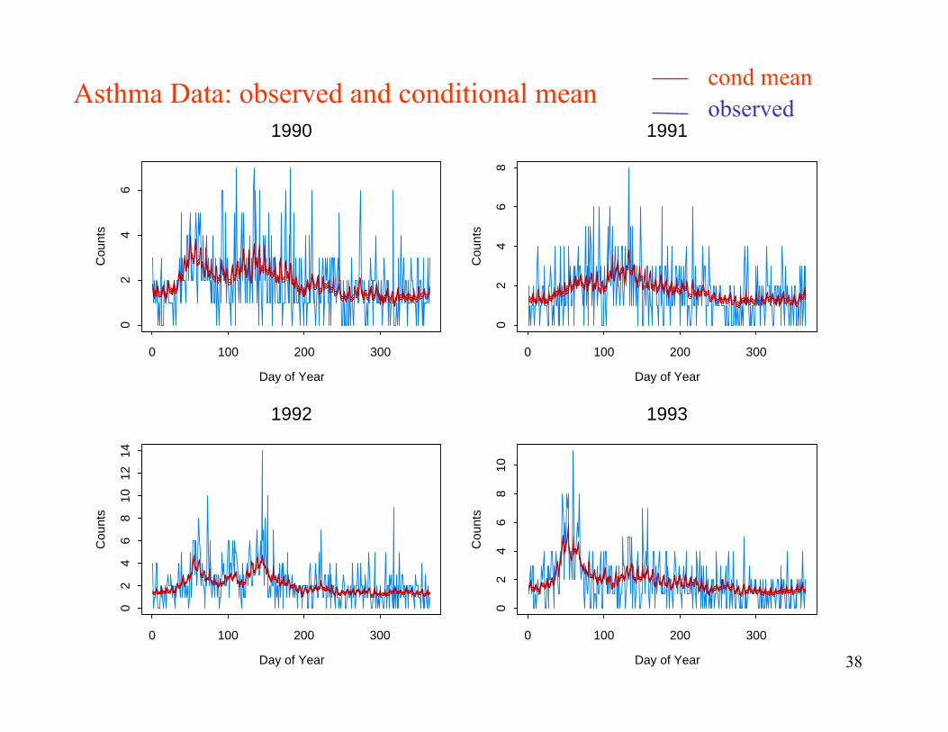
Asthma Data: observed and conditional mean cond meanobserved
1990
Day of Year
Cou
nts
0 100 200 300
02
46
1991
Day of Year
Cou
nts
0 100 200 300
02
46
8
1992
Day of Year
Cou
nts
0 100 200 300
02
46
810
1214
1993
Day of Year
Cou
nts
0 100 200 300
02
46
810
39
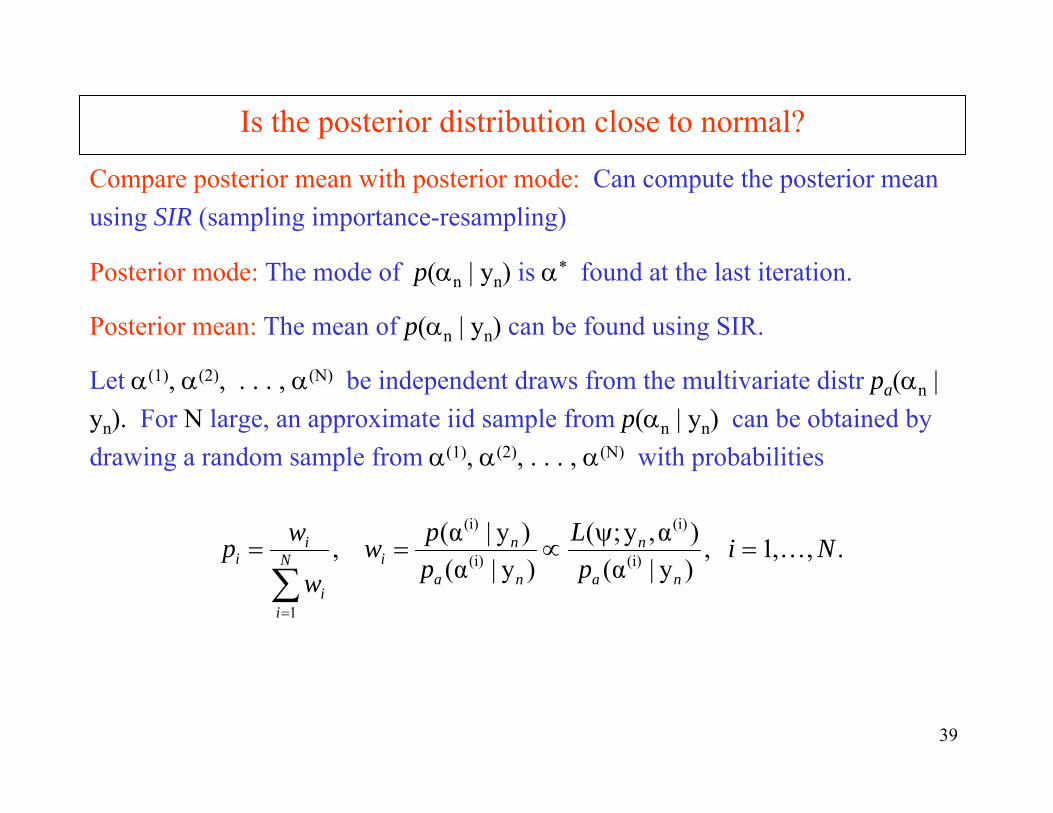
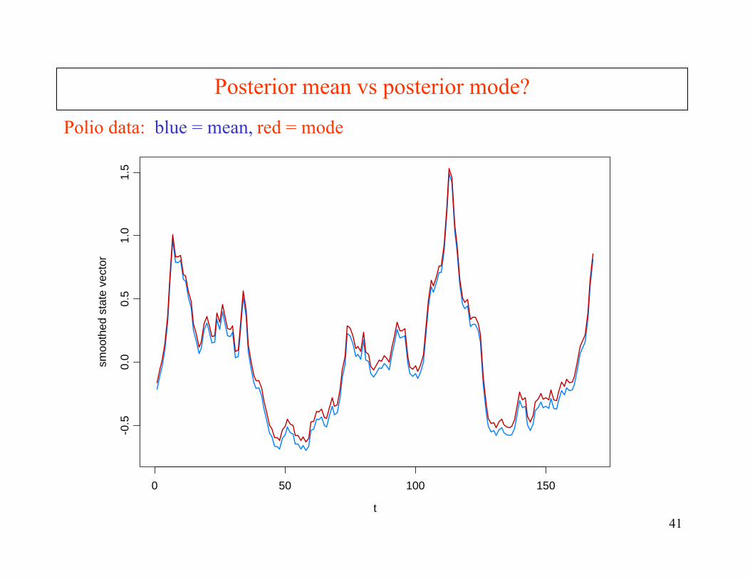
Is the posterior distribution close to normal?
Compare posterior mean with posterior mode: Can compute the posterior mean using SIR (sampling importance-resampling)
Posterior mode: The mode of p(αn | yn) is α* found at the last iteration.
Posterior mean: The mean of p(αn | yn) can be found using SIR.
Let α(1), α(2), . . . , α(N) be independent draws from the multivariate distr pa(αn | yn). For N large, an approximate iid sample from p(αn | yn) can be obtained bydrawing a random sample from α(1), α(2), . . . , α(N) with probabilities
.,,1 ,)y|(α)α,y;(
)y|(α)y|(α , (i)
(i)
(i)
(i)
1
Nip
Lppw
w
wpna
n
na
niN
ii
ii K=
ψ∝==
∑=
41
Posterior mean vs posterior mode?
Polio data: blue = mean, red = mode
t
smoo
thed
sta
te v
ecto
r
0 50 100 150
-0.5
0.0
0.5
1.0
1.5
44
Summary Remarks
1. Importance sampling offers a nice clean method for estimation in parameter driven models.
2. The innovations algorithm allows for quick implementation of importance sampling. Extends easily to higher-order AR structure.
3. Relative likelihood approach is a one-sample based procedure.
4. Approximation to the likelihood is a non-simulation based procedure which may have great potential especially with large sample sizes and/or large number of explanatory variables.
5. Approximation likelihood approach is amenable to boostrapping procedures for bias correction.