revisiting the ramachandran plot: hard-sphere repulsion

Revisiting the Ramachandran plot: Hard-sphererepulsion, electrostatics, and H-bonding in the �-helix

BOSCO K. HO,1 ANNICK THOMAS,2 AND ROBERT BRASSEUR1

1Centre de Biophysique Moléculaire Numérique (CBMN), B-5030 Gembloux, Belgium2Institut National de la Santé et de la Recherche Médicale (INSERM), 75013 Paris, France

(RECEIVED June 2, 2003; FINAL REVISION July 14, 2003; ACCEPTED July 16, 2003)

Abstract

What determines the shape of the allowed regions in the Ramachandran plot? Although Ramachandranexplained these regions in terms of 1–4 hard-sphere repulsions, there are discrepancies with the data where,in particular, the �R, �L, and �-strand regions are diagonal. The �R-region also varies along the �-helixwhere it is constrained at the center and the amino terminus but diffuse at the carboxyl terminus. Byanalyzing a high-resolution database of protein structures, we find that certain 1–4 hard-sphere repulsionsin the standard steric map of Ramachandran do not affect the statistical distributions. By ignoring these stericclashes (N···Hi+1 and Oi−1···C), we identify a revised set of steric clashes (C�···O, Oi−1···Ni+1, C�···Ni+1,Oi−1···C�, and Oi−1···O) that produce a better match with the data. We also find that the strictly forbiddenregion in the Ramachandran plot is excluded by multiple steric clashes, whereas the outlier region isexcluded by only one significant steric clash. However, steric clashes alone do not account for the diagonalregions. Using electrostatics to analyze the conformational dependence of specific interatomic interactions,we find that the diagonal shape of the �R and �L-regions also depends on the optimization of the N···Hi+1

and Oi−1···C interactions, and the diagonal �-strand region is due to the alignment of the CO and NH dipoles.Finally, we reproduce the variation of the Ramachandran plot along the �-helix in a simple model that usesonly H-bonding constraints. This allows us to rationalize the difference between the amino terminus and thecarboxyl terminus of the �-helix in terms of backbone entropy.

Keywords: Ramachandran plot; �-helix; hard-sphere model; H-bonds

In 1963, Ramachandran et al. introduced the �–� angles(Fig. 1A) as a parameterization of the protein backbone. Theplot of these angles, the Ramachandran plot, has become astandard tool used in determining protein structure (Morriset al. 1992; Kleywegt and Jones 1996) and in defining sec-ondary structure (Chou and Fasman 1974; Muñoz and Ser-rano 1994). Using an analysis of local hard-sphere repul-sions between atoms that are at least third neighbors (1–4interactions), Ramachandran et al. (1963) constructed asteric map of the Ramachandran plot that predicted the com-monly allowed regions: the �R, �L, and �-regions. Thissteric map (Fig. 1B) has become the standard interpretation

of the Ramachandran plot (Richardson 1981) where Mandelet al. (1977) identified the specific steric clashes that definethe boundaries of the standard steric map.

However, there are differences with the data. Using ahigh-resolution (<1.8 Å) database of structures with asample size of nearly 100,000 residues (Lovell et al. 2003),we can see differences between the observed Ramachandranplot (Fig. 2A) and the standard steric map (see Fig. 1B). The�R and �L regions are diagonal (Garnier and Robson 1990;Hovmöller et al. 2002). The �-region partitions into twodiagonal lobes: the �-strand region (left) and the polypro-line II region (right; Kleywegt and Jones 1996; Hovmölleret al. 2002). There also exists sparsely populated regionsthat are forbidden in the standard steric map such as the �and �� regions (Milner-White 1990), the type II turn region(Sibanda and Thornton 1985), and the pre-Pro region(Macarthur and Thornton 1991).

Reprint requests to: Bosco K. Ho, Centre de Biophysique MoléculaireNumérique (CBMN), 2 Passage des déportés, B-5030 Gembloux, Belgium;e-mail: [email protected]; fax: +32-81-622-522.

Article and publication are at http://www.proteinscience.org/cgi/doi/10.1110/ps.03235203.

Protein Science (2003), 12:2508–2522. Published by Cold Spring Harbor Laboratory Press. Copyright © 2003 The Protein Society2508

Various studies have refined the calculation of the Ra-machandran plot by using Lennard-Jones potentials and elec-trostatics (for a review, see Ramachandran and Sasisekharan1968). Nevertheless, electrostatics fail to adequately repro-duce the Ramacahandran plot (Lovell et al. 2003). In par-ticular, the origin of the diagonal shape of the �R, �L, and�-strand regions is not well understood. Furthermore, Hu etal. (2003) showed that typical molecular mechanics (MM)force fields generate unrealistic Ramachandran plots. Incontrast, they modeled the alanine dipeptide using quantummechanics (QM), which they placed in an explicit solventmodeled with MM. They reproduced the observed Rama-chandran plot, showing that the Ramachandran plot arisesfrom local backbone interactions.

Is there a simple way to account for the boundaries of theobserved Ramachandran plot? To this end, we have ana-lyzed the statistical distributions of the interatomic distances

parameterized by the �–� angles. We found that certain 1–4steric clashes in the standard steric map have no discernibleeffect on the statistical distributions. By ignoring theseclashes, we can analyze the contributions of the remainingsteric clashes. We thus obtain a revised steric map thatproduces a better match to the observed Ramachandran plot.

However, steric clashes do not account for the diagonalshape of the �R-region. The standard steric map predicted asmaller �R-region (see Fig. 1B) than the observed �R-region(Fig. 2A). However, the predicted �R-region is also elon-gated horizontally into regions where there is no observeddensity. Another problem is why the Ramachandran plot ofresidues in �-helices is constrained to the lower half of thegeneral �R-region (Fig. 2B). It is often stated (Karplus1996) that the �R-region consists of two discrete regions:the helical �R-region and the �R-region. In this study, weattempt to clarify the relationship between the general �R-region and the helical �R-region.

Given that the strong diagonal shape of the observed�R-region has been reproduced by QM calculations (Hu etal. 2003), the shape of the �R-region must be due to localbackbone interactions. Lovell et al. (2003) argued that thediagonal �R-region is due to the disfavoring of the confor-mations near (−150°, −60°) where the H and Hi+1 atoms areclose together. However, we find that crowded H and Hi+1

atoms are also found in favored conformations of the �R-region, for example (−110°, 0°). As the crowding of Hatoms produces different results in different parts of theRamachandran plot, something else must induce the diago-nal shape of the �R-region.

We use electrostatics to analyze the conformational de-pendence in the Ramachandran plot of specific interatomicinteractions. We find that various dipole–dipole interac-tions, when combined with the revised steric map, confor-mationally induce diagonal �R, �L, and �-strand regions.Although, in general, electrostatics cannot account for theRamachandran plot (Lovell et al. 2003), the conformationaldependence of individual interatomic interactions in the Ra-machandran plot cannot differ greatly between electrostaticsand QM. After all, only atoms with opposite partial chargesattract and like charges repel. However, as the strength ofindividual interactions can vary greatly in the QM calcula-tion, the electrostatic approximation fails when all the indi-vidual minima are summed together.

Recent studies have found that the shape of the helical�R-region varies depending on the position of the residue inthe �-helix. In the central residues and in the amino termi-nus, the helical �R-region is constrained to the lower half ofthe general �R-region. However, Petukhov et al. (2002)found that the Ramachandran plot at the carboxyl terminusis much more diffuse than the rest of the �-helix. Thisflexibility in the carboxyl terminus has also been observedin peptide studies (Miick et al. 1993). In simulations, thereis an asymmetry between the amino terminus and the car-

Figure 1. Schematic of the �–� angles. (A) The schematic of the alaninedipeptide that represents the protein backbone parameterized by the� � ∠ C-N-C�-C and � � ∠ N-C�-C-N dihedral angles. (B) The originalRamachandran steric map (Ramachandran et al. 1963) where the specifichard-sphere repulsions (dashed line) identified by Mandel et al. (1977)define the allowed regions (gray): �L, �R, and � regions.

Revisiting the Ramachandran plot

www.proteinscience.org 2509

boxyl terminus in both folding (Sung 1994; Voegler-Smithand Hall 2001) and unfolding (Soman et al. 1991) studies.The origin of this asymmetry has not yet been resolved.

Ramachandran and Sasisekharan (1968) showed that H-bonding constraints induce the constrained helical �R-re-gion. They analyzed �-helices where all residues were pa-rameterized with the same �–� angles. They identified the�–� angles where d(Oi···Hi+4) ∼ 2.0 Å for all CO···HN H-bonds along the �-helix. These �–� angles correspond tothe constrained helical �R-region in central helical residues.However, as the analysis of Ramachandran and Sasisekha-ran (1968) used �-helices that had identical �–� angles, thisonly accounts for central helical residues. What then causesthe differences between the amino terminus and the car-boxyl terminus? We first analyzed the Ramachandran plots

along different positions of the �-helix in the structuraldatabase. Then, using an extension of the model of Ra-machandran and Sasisekharan (1968), we studied the con-straints of the backbone H-bonding along the �-helix. Asour model reproduced the observed variation along the�-helix, we can use backbone H-bonding to explain theobserved differences between the amino terminus and thecarboxyl terminus of the �-helix.

Materials and methods

Data set

We used the data set of 500 nonhomologous proteins (Lovell et al.2003) from the PDB (Bernstein et al. 1977) with resolution better

Figure 2. Ramachandran plots. (A) All residues excluding Pro, Gly, and pre-Pro; (B) residues in the center of the �-helix, which aremore constrained than for all residues; (C) the Ncap residue; and (D) the Ccap residue in the �-helix, which are scattered throughoutthe entire allowed region.

Ho et al.

2510 Protein Science, vol. 12

than 1.8 Å. In this data set, all hydrogen atoms have been projectedfrom the backbone and optimized. Due to their specialized Ra-machandran plots, we excluded Gly, Pro, and pre-Pro residues(MacArthur and Thornton 1991) from our analysis. In the stericclash analysis, we used the van der Waals (vdW) radii given by theRichardson lab (Word et al. 1999) (H� � 1.17 Å, H � 1.00 Å,C � 1.65 Å, C� and C� � 1.75 Å, O � 1.40 Å, and N � 1.55Å). We used DSSP (Kabsch and Sander 1983) to define �-helicalresidues.

Local conformations of the �–� map

To calculate the ideal curves of the interatomic distances as afunction of the �-� angles, we modeled the alanine dipeptide (seeFig. 1A). Covalent bond lengths and angles were fixed to standardEngh and Huber (1991) values, which only allows the �–� anglesto vary. The �–� angles of the central residue were incremented in5° steps and the corresponding distance parameters were calcu-lated. Then, we generated the energy map of the Ramachandranplot by calculating, for each value of �–�, the energy of variousinteratomic interactions. We used two types of interactions: partialcharge electrostatics

Eelec � 331 * (q1*q2/d) kcal.mole−1,

and Lennard-Jones 12–6 potentials

ELJ � � [(�/d)12 − 2 (�/d)6] kcal.mole−1,

where the parameters were taken from CHARMM22 (MacKerellJr. et al. 1998).

Model of �-helix

We modeled the �-helix with a chain of 7 Ala residues. Covalentbond lengths and angles were fixed to standard Engh and Huber(1991) values where the �–� angles are the only degrees of free-dom. As the �–� angles of the Ncap and Ccap do not affect thegeometry of the H-bonds within the �-helix, they were ignored.

The simplest requirement to form CO···HN H-bonds is thatd(O···H) ∼ 2.0 Å. Thus, to impose a given CO···HN H-bond, weused a harmonic distance constraint to minimize the O···H dis-tance:

ECO···HN � (d[O···H] − 2.0 Å)2.

The minimum of this constraint is zero when d[O···H] � 2.0 Å.We also used ECO···HN to measure the deviation from the idealCO···HN H-bond geometry when the given conformation cannotform the CO···HN H-bond. To avoid steric clashes, we appliedLennard-Jones 12–6 potentials:

ELJ � � ([�/d]12 − 2 [�/d]6) kcal.mole−1,

where the parameters were taken from CHARMM22 (MacKerrellJr. et al. 1998).

To analyze the H-bonding constraints in the amino terminalresidues (N1, N2, and N3; red in Fig. 8B, below), we fixed the �–�angles of N4, N5, and N6 to the average helical values (−63°,−42°), which assumes that the �-helix from N4 to the carboxy-terminal is fixed in the �-helical conformation. We then minimizedthe energy function:

E � i EL-J,i + j ECO···HN,j,

where the first term refers to the Lennard-Jones potential, whichmodels the steric clashes, and the second term refers to the har-monic potentials that minimizes the CONc···HNN4, CON1···HNN5,and CON2···HNN6 H-bonds (red in Fig. 8B, below).

(1) For N1, we divided the Ramachandran plot into a grid ofpoints separated by 5° intervals. For each grid point, we usedPowell minimization (Press et al. 1986) to minimize E byvarying the �–� angles of the N2 and N3 residues. We re-peated the process for all grid points of N1 to generate anenergy profile of N1.

(2) For the grid points of N2, we allow the �–� angles of N1 andN3 to vary.

(3) For the grid points of N3, we allow the �–� angles of N1 andN2 to vary.

To analyze the H-bonding constraints in the carboxy-terminal resi-dues (C1, C2, and C3; red in Fig. 8A, below), we fixed the �–�angles of C4, C5, and C6 to the average helical values of (−63°,−42°), which assumes that the �-helix from C4 to the aminoterminus is fixed in �-helical conformation. In the energy min-imization, we modeled the COC4···HNCc, COC5···HNC1, andCOC6···HNC2 H-bonds (red in Fig. 8A, below).

(1) For the grid points of C3, we allow the �–� angles of C2 andC1 to vary.



Results and Discussion

Because the database of protein structures contains a largenumber of residues (97,368), we can compare the statisticaldistributions directly to the ideal geometry of the proteinbackbone. The local interatomic distances that are directlyparameterized by the �–� angles can be divided into threecategories: � dependent, � dependent, and �-� codependentdistances. In Table 1, we list the parameters of these inter-atomic distances. By comparing the value of the 5% mini-mum (5th percentile band) with the vdW diameter, we cansee which atoms are in contact and can interact. We focuson the steric clashes of the standard steric map (Rama-chandran and Sasisekharan 1968). As described in Mandelet al. (1977), they are: Oi−1···C and Oi−1···C�, which restricts�; N···Hi+1 and C�···Hi+1, which restricts �; and O···Hi+1,H···Hi+1 and Oi-1···O, which shaves off the corners of theallowed regions (see Fig. 1B).

The � dependent and � dependent steric constraints

The �-dependent distances

We first consider the restrictions from the standard stericmap that restrict �: Oi−1···C� and Oi−1···C (see Fig. 1B). Toevaluate the effect of each steric clash on the observed



distribution, we can make two comparisons. First, we cancompare the � frequency distributions to the ideal curve.The idea is that if a hard-sphere repulsion restricts �, then,in regions of � where the ideal curve is below the vdWdiameter, the � frequency distribution should drop corre-spondingly. Distributions that are found below the vdWradius indicates a steric overlap that could be due to somekind of interaction. For example, Ho and Curmi (2002)showed that in the allowed regions of � in �-sheet residues,there is an Oi−1···H� nonbonded electrostatic interactionwhere most of the observed values are found below the vdWdiameter (Fig. 3A). We plot the observed frequency distri-bution of � at the bottom of Figure 3. For the ideal curvesof both d(Oi−1···C�) versus � (Fig. 3D) and d(Oi−1···C) ver-sus � (Fig. 3B), we see that as the interatomic distancedecreases below the vdW diameter, the � frequency distri-bution drops correspondingly. This is consistent with theOi−1···C� and Oi−1···C steric clashes restricting the � angle.

Second, we can compare the observed distributionsagainst the ideal curves based on standard geometry (see

Materials and Methods). Deviation of the observed distri-bution from the ideal curve indicates possible steric strain.The observed distributions of d(Oi−1···C) versus � (Fig. 3B)and d(Oi−1···C�) versus � (Fig. 3D) fit the ideal curves well,showing that there are no significant deviations from stan-dard geometry.

The �-dependent distancesIn the standard steric map, it is the N···Hi+1 steric clash

that restricts � in the region 0° < � < 90° (see Fig. 1B).Comparing the ideal curve of d(N···Hi+1) versus � to the �frequency distribution (bottom of Fig. 4), we see that thereis no corresponding drop in the � frequency distribution asd(N···Hi+1) descends below its vdW diameter (Fig. 4C). TheN···Hi+1 steric clash has no effect on the � angle. Further-more, the observed distribution of d(N···Hi+1) versus � isdistorted from the ideal curve for the region whered(N···Hi+1) is below the vdW diameter. Karplus (1996) hasshown that this deviation accommodates the close approachof the N···Hi+1 interaction. On the other hand, we find that

Table 1. Range of the interatomic distances [Å] parameterized by the �–� angles

vdW 5% 95% �L �R �

� dependent parametersH···H� 2.17 2.74 2.98 2.20 ± 0.09 2.84 ± 0.06 2.92 ± 0.06H···C� 2.75 2.43 3.01 3.13 ± 0.09 2.52 ± 0.10 2.69 ± 0.18H···C 2.65 2.53 3.22 3.18 ± 0.12 3.09 ± 0.14 2.79 ± 0.22Oi−1···H� 2.57 2.26 2.85 3.83 ± 0.12 2.60 ± 0.18 2.45 ± 0.15Oi−1···C� 3.15 3.32 4.30 3.09 ± 0.17 4.19 ± 0.15 3.92 ± 0.30Oi−1···C 3.05 2.85 4.11 3.01 ± 0.25 3.14 ± 0.31 3.66 ± 0.40Ci−1···C 3.30 2.96 3.62 3.07 ± 0.13 3.12 ± 0.17 3.36 ± 0.21Ci−1···C� 3.40 3.20 3.75 3.08 ± 0.09 3.68 ± 0.09 3.53 ± 0.17

� dependent parametersH�···O 2.57 2.47 3.30 2.93 ± 0.16 2.57 ± 0.11 3.24 ± 0.06C�···O 3.15 2.82 3.40 2.86 ± 0.25 3.21 ± 0.17 3.12 ± 0.16N···O 2.95 2.67 3.63 3.49 ± 0.21 3.53 ± 0.13 2.82 ± 0.14H�···Hi+1 2.17 2.20 3.69 2.92 ± 0.28 3.55 ± 0.18 2.33 ± 0.13C�···Hi+1 2.75 2.96 3.97 3.89 ± 0.43 3.33 ± 0.29 3.45 ± 0.29N···Hi+1 2.55 2.34 3.99 2.67 ± 0.39 2.55 ± 0.23 3.78 ± 0.22H�···Ni+1 2.72 2.46 3.33 2.85 ± 0.17 3.24 ± 0.12 2.54 ± 0.08C�···Ni+1 3.30 3.03 3.66 3.61 ± 0.25 3.25 ± 0.17 3.32 ± 0.19N···Ni+1 3.10 2.70 3.64 2.89 ± 0.22 2.81 ± 0.13 3.50 ± 0.15

�-� co-dependent parametersOi−1···O 2.80 3.27 4.85 3.61 ± 0.42 3.73 ± 0.46 4.34 ± 0.51Ci−1···O 3.05 3.31 4.50 3.93 ± 0.30 4.02 ± 0.27 3.80 ± 0.32H···Hi+1 2.17 2.40 4.64 3.03 ± 0.50 2.72 ± 0.29 4.42 ± 0.22H···Ni+1 2.55 2.91 4.30 3.43 ± 0.29 3.21 ± 0.21 4.00 ± 0.23Ci−1···Hi+1 2.65 2.70 4.82 3.09 ± 0.50 3.11 ± 0.35 4.31 ± 0.43Ci−1···Ni+1 3.15 3.11 4.63 3.31 ± 0.31 3.35 ± 0.25 4.19 ± 0.34Oi−1···Hi+1 2.40 3.00 4.82 3.37 ± 0.50 3.59 ± 0.39 4.05 ± 0.59Oi−1···Ni+1 2.95 3.13 4.87 3.33 ± 0.36 3.54 ± 0.37 4.16 ± 0.54O···H 2.40 2.38 4.34 4.20 ± 0.32 4.20 ± 0.24 2.81 ± 0.36

Minimum–maximum values are defined by the 5th–95th percentile bands. The criteria to define the regions in theRamachandran plot are �L: � > 0°; �R: � < 0° and � < 50°; and �: � < 0° and � > 50°. The average and standarddeviation for the interatomic distances are also given for each region. The average (�, �) for each region are �L � (61°,26°); �R � (−73°, −33°); and � � (−108°, 136°). Comparing the 5% minimum of the distances with the correspondingvdW radius indicates possible steric clashes.

Ho et al.


the ideal curve of d(C�···O) versus � corresponds quite wellto the variation of the � frequency distribution (Fig. 4D).This suggests that in the region 0° < � < 90°, we can ignorethe effects of the N···Hi+1 steric clash and instead, use theC�···O steric clash. Indeed, given that the N···Hi+1 interac-tion deviates from the ideal geometry, the position of theHi+1 atom is somewhat flexible.

Figure 3. Distributions of interatomic distances [Å] parameterized by �

[°]. The ideal curves (gray) are calculated using Engh and Huber (1991)geometry. The vdW diameters (dashed line) are taken from Word et al.(1999). (A) Oi−1···H� versus �; (B) Oi−1···C versus �; (C) Ci−1···C� versus�; and (D) Oi−1···C� versus �. The � frequency distribution is shown at thebottom of D.

Figure 4. Distributions of interatomic distances [Å] parameterized by �

[°]. The ideal curves (gray) are calculated using Engh and Huber (1991)geometry. The vdW diameter (dashed line) are taken from Word et al.(1999). (A) C�···Hi+1 versus �; (B) C�···Ni+1 versus �; (C) N···Hi+1 versus�; and (D) C�···O versus �. The � frequency distribution is shown at thebottom of D.



In the standard steric map, it is the C�···Hi+1 steric clashthat restricts � in the region −180° < � < −50° (see Fig. 1B).In the comparison of the � frequency distribution (bottom ofFig. 4) to the ideal curve of d(C�···Hi+1) versus �, theC�···Hi+1 steric clash appears to restrict � (Fig. 4A). How-ever, the observed 5% minimum value of d(C�···Hi+1) is0.21 Å higher than the vdW diameter (Table 1), suggestingthat the C�···Hi+1 steric clash is not responsible for the re-striction on �. Is there any other interaction that could beresponsible? The ideal curve of d(C�···Ni+1) versus � alsocorresponds to the drop-off in the � distribution (Fig. 4B).However, the observed 5% minimum value of C�···Ni+1 isbelow the vdW diameter (Table 1), which is a clear stericcontact. Hence, we should ignore the C�···Hi+1 steric clashand replace it with the C�···Ni+1 steric clash. Furthermore,as the H atom is more flexible than the other backboneatoms and the H atom has a negligible vdW interaction, weexpect that the C�···Hi+1 interaction will be soft and notbehave as a hard steric clash.

The �–� codependent distances

However, if we look at interatomic distances as a functiononly of �, or as a function only of �, then we will miss stericclashes that are �–� codependent. For example, in the stan-dard steric map, the Oi−1···C steric clash excludes the middleof the Ramachandran plot, resulting in vertical boundariesin the �, �L, and � regions (see Fig. 1B). However, thesevertical boundaries are not found in the observed distribu-tion, where the corresponding boundaries are diagonal (seeFig. 2A). Because the �–� codependent steric clashes in-duce diagonal boundaries, if we ignore the Oi−1···C stericclash, then we can identify the steric clashes that inducediagonal boundaries (Fig. 5A).

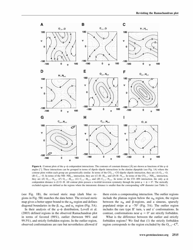
To make the comparison with the data, we generate allthe contour plots of constant distance for the �–� codepen-dent interactions. We show these contour plots in Figure 6mainly as a reference. We then define the steric boundariesof each contour plot by considering the regions where thedistances are smaller than the corresponding vdW diameter(Table 1). In Figure 5A, we identify the steric clashes thatbest match the diagonal boundaries of the observed distri-bution. These diagonal boundaries exclude a region in theRamachandran plot that runs down the middle of the plot.This excluded region can be divided into two. The firstregion, excluded by the Oi−1···O steric clash, consists ofboth the upper-central and lower-central regions, which aresymmetric due to the inversion symmetry found in all thecontour maps (Fig. 6). The second region, excluded by theOi−1···Ni+1 steric clash, is in the center of the Ramachandranplot.

The revised steric map of the Ramachandran plot

From the analysis above, we find that the N···Hi+1 stericclash does not affect the frequency distributions of � and

that ignoring the Oi−1···C steric clash results in well-defineddiagonal boundaries in the Ramachandran plot. Thus, weobtain a revised set of steric clashes where (1) the Oi−1···C�

steric clash restricts �; (2) the C�···O and C�···Ni+1 stericclashes restrict �; and (3) the Oi−1···O and O···Ni+1 stericclashes restrict �–�. Compared to the standard steric map

Figure 5. Revised steric map. (A) The steric clashes (dashed blue lines)that best match the data. d(Oi−1···O) � 2.7Å, d(Oi−1···Ni+1) � 2.7 Å, andd(H···Hi+1) � 1.6 Å. (B) Schematic of the revised steric map showingsteric restrictions (dashed blue lines) and sterically allowed regions (darkblue). The revised steric map gives diagonal boundaries for the �R, �L, and� regions and defines a more realistic upper boundary for the �R-region.Diagonal �R and �L regions (red region) from the dipole–dipole analysis(Fig. 7G) are defined mainly by the attractive Oi−1···C and N···Hi+1 inter-actions (red lines). The diagonal �-strand region (yellow) is induced byaligning the CO···HN dipole–dipole interaction. Regions that are only ex-cluded by a single steric clash (light blue) accounts for the outlier region inLovell et al. (2003).

Ho et al.


(see Fig. 1B), the revised steric map (dark blue re-gions in Fig. 5B) matches the data better. The revised stericmap gives a better upper bound to the �R-region and definesdiagonal boundaries in the �, �R, and �L region (Fig. 5A).

In their analysis of the �–� distribution, Lovell et al.(2003) defined regions in the observed Ramachandran plotin terms of favored (98%), outlier (between 98% and99.5%), and strictly forbidden regions. In the outlier region,observed conformations are rare but nevertheless allowed if

there exists a compensating interaction. The outlier regionsinclude the plateau region below the �R region, the regionbetween the �R and �-regions, and a sinuous, sparselypopulated stripe at � ∼ 70° (Fig. 5A). The outlier regionincludes the rare type II� turn, � and �� conformations. Incontrast, conformations near � � 0° are strictly forbidden.

What is the difference between the outlier and strictlyforbidden regions? We find that (1) the strictly forbiddenregion corresponds to the region excluded by the Oi−1···C�,

Figure 6. Contour plots of the �–� codependent interactions. The contours of constant distance [Å] are shown as functions of the �–�

angles [°]. These interactions can be grouped in terms of dipole–dipole interactions in the alanine dipeptide (see Fig. 1A) where thecontour plots within each group are geometrically similar. In terms of the COi−1···CO dipole–dipole interaction, they are (A) Oi−1···O,(B) Ci−1···O. In terms of the NH···NHi+1 interaction, they are (C) H···Hi+1 and (D) H···Ni+1. In terms of the COi−1···NHi+1 interaction,they are (E) Oi−1···Ni+1, (F) Oi−1···Hi+1, (G) Ci−1···Hi+1, and (H) Ci−1···Ni+1. In terms of the CO···HN interaction, the only �–�

codependent distance is (I) O···H. All contour plots possess a twofold inversion symmetry through the point � � � � 0°. The stericallyexcluded regions are defined as the regions where the interatomic distance is smaller than the corresponding vdW diameter (see Table 1).



Oi−1···O, and O···Ni+1 steric clashes; and (2) the outlier re-gion is excluded by the C�···O and C�···Ni+1 steric clashes.Although we have identified only a single steric clash that isinduced by diagonal boundaries in Figure 5B, some of theboundaries are in fact induced by multiple steric clashes.The existence of multiple hard steric clashes accounts forthe difference between the strictly forbidden and outlierregions. The multiple steric clashes exist because we cangroup the �–� codependent distances in terms of the di-pole–dipole interactions in the alanine dipeptide (see Fig.1A). The contour plots that belong to each dipole–dipoleinteraction are geometrically similar (Fig. 6).

In the strictly forbidden region of the Ramachandran plot(white in Fig. 5B), both the Oi−1···O (Fig. 6A) and Ci−1···O(Fig. 6B) steric clashes exclude the same �–� region. Wefind that all the interatomic interactions that are groupedwithin the COi−1···NHi+1 interaction dipole–dipole interac-tions (Oi−1···Ni+1, Oi−1···Hi+1, Ci−1···Hi+1, and Ci−1···Ni+1)exclude the same central region in the Ramachandran plot(Fig. 6E–H). We also find that both the Oi−1···C� steric clash(see Fig. 3D) and Ci−1···C� steric clash (see Fig. 3C) excludethe same region of � where the Ci−1···C� interaction is in aparticularly serious steric overlap. This steric overlap couldbe an indication that the vdW radius of C (Word et al. 1999)is overestimated or that the electron shell of C is not entirelyspherical.

In contrast, the outlier region corresponds to the regionrestricted by a single steric clash (light blue in Fig. 5B). Forthe region 0° < � < 90°, only the C�···O steric clash restricts� (see Fig. 4D). It is not reinforced by N···Hi+1 (see Fig. 4C)as the N···Hi+1 interaction is not a hard steric clash. In theother region −180° < � < −50°, as C�···Hi+1 is probably nota hard steric clash (see Fig. 4A), only the C�···Ni+1 stericclash (Fig. 4B) restricts �.

Local electrostatic interactionsin the Ramachandran plot

However, not all the features of the observed Ramachandranplot can be explained by local steric clashes. In this section,we focus on the diagonal shapes of the �R, �L, and �-strandregion. In previous studies, the � and �� regions were ex-plained in terms of a C7 H-bond (Milner-White 1990). Thepolyproline II region within the �-region was explained interms of both a favorable COi−1···CO interaction (Maccal-lum et al. 1995) and as the most entropically favored con-formation (Pappu and Rose 2002). Ho and Curmi (2002)showed that restrictions due to hydrogen bonds in �-sheetformation induce a diagonal �-strand region. However, thediagonal shape of the �-strand region is also induced forresidues not in �-sheets. Therefore, the diagonal �-strandregion must also arise from local backbone interactions.

Lovell et al. (2003) argued that the diagonal �R-region isdue to the disfavoring of the conformations near (−150°,

−60°) (Fig. 5A), where the H and Hi+1 atoms are closetogether. They postulated that the crowding of the H atomsis disfavored because this prevents the formation of oneH-bond with the solvent. However, comparing the contourdistance plot of H···Hi+1 (Fig. 6C) with the observed �R-region (see Fig. 2A), we can see that favored conformationsin the observed plot, such as (−110°, 0°), also has crowdedH and Hi+1 atoms. As the crowding of H atoms producesdifferent results in different parts of the Ramachandran plot,something else must induce the diagonal shape of the �R-region.

Following Maccallum et al. (1995), we analyze the elec-trostatic interactions of the alanine peptide in terms of thedipole–dipole interactions: the COi−1···CO, NH···NHi+1,COi−1···NHi+1, and CO···NH interactions. The differencewith the study of Maccallum et al. (1995) is that in ourcalculation, we have included the Lennard-Jones potentialsof our revised set of steric clashes (Fig. 7A).

The combined electrostatic map (Fig. 7B) does not pro-duce a minimum in the �R-region. However, when consid-ered individually, we find that, of the four dipole–dipoleinteractions, the COi−1···CO (Fig. 7C), NH···NHi+1 (Fig.7D), and CO···NH (Fig. 7E) interactions induce diagonalshapes in the �R and �L regions. Consequently, the energymap that combines the COi−1···CO, NH···NHi+1, andCO···NH interactions (Fig. 7G) produces well-defined di-agonal minima in the �R and �L regions. In the backboneconformation of these regions (the diagram in Fig. 1A cor-responds to such a conformation), (1) the COi−1 dipolepoints toward the CO dipole such that Oi−1 is in contact withC; (2) the NHi+1 dipole points toward the NH dipole suchthat the N atom is in contact with the Hi+1 atom; and (3) theCO and NH groups are aligned in an antiparallel conforma-tion such that O is as far away from H as possible. A simpledescription of this conformation is that the Oi−1···C andN···Hi+1 attraction are simultaneously optimized. Optimiz-ing the Oi−1···C interaction will restrict |�| < 100°, and op-timizing the N···Hi+1 interaction will restrict |�| < 80° (seeFig. 5B). The optimization of the N··· Hi+1 interaction in the�R-region was also observed by Karplus (1996).

Maccallum et al. (1995) showed that the polyproline IIregion corresponds to a minimum in the electrostaticCOi−1···CO interaction. We can see this in Figure 7C. Simi-larly, we find that the diagonal �-strand region can also beexplained in terms of an electrostatic dipole–dipole interac-tion. A diagonal minimum of the CO···NH is induced (Fig.7E), which corresponds to the observed �-strand region (seeFig. 5A). In this minimum, the CO and NH groups in thebackbone are essentially aligned and co-planar. ThisCO···HN electrostatic minimum is so deep that the diagonal�-strand region is still found in the combined electrostaticinteraction (Fig. 7B).

Although it has been shown that the COi−1···NHi+1 inter-action induces the � and �� region (Milner-White 1990), the

Ho et al.


Figure 7. Contour plots of the dipole–dipole interactions [kcal/mole] as a function of the �–� angles [°]. Energy plots of (A) the Lennard-Jones 12–6potentials of the revised set of steric clashes; (B) all electrostatic interactions; the individual dipole–dipole interactions of (C) COi−1···CO; (D) NH···NHi+1;(E) CO···NH; and (F) COi−1···NHi+1. (G) The combination of the COi−1···CO, NH···NHi+1 and CO···NH dipole–dipole interactions produces clear diagonalminima in the �R, �L, and � regions.



electrostatic approximation of the COi−1···NHi+1 interactiondoes not induce a minimum in the � region (Fig. 7F). How-ever, it does induce a weak minimum in the �� region.Compared to the QM calculcations (Hu et al. 2003), theelectrostatic approximation of the COi−1···NHi+1 interactionis poor, which is probably the reason why the combinedelectrostatic map (Fig. 7B) does not give the diagonal �R-region.

Ramachandran plots of the �-helix

Although the Ramachandran plot of residues in �-helices isfound within the �R-region (Ramachandran and Sasisekha-ran 1968), there are subtle but significant differences. TheRamachandran plot of residues in the center of the �-helixis smaller than the �R-region and the Ramachandran plotvaries at different positions of the �-helix termini (Petukhovet al. 2002). We use the Richardson and Richardson termi-nology (1988) to describe the different positions of the�-helical residues. The residues at the amino terminus arelabeled Ncap-N1-N2-N3-N4–··· (Fig. 8B) where the amino-terminal residues (N1, N2, N3) only contribute CO groupsto H-bonds. The residues at the carboxyl terminus are la-beled ···C4-C3-C2-C1-Cap (Fig. 8A) where the carboxy-terminal residues (C1, C2, C3) only contribute NH groupsto H-bonds. Ccap and Ncap are boundary residues, whichare not considered part of the �-helix.

Here, we plot the Ramachandran plots of the �-helicalresidues: Ncap (see Fig. 2C), N1, N2, N3 (Fig. 9), central(see Fig. 2B), C3, C2, C1 (Fig. 10), and Ccap (see Fig. 2D).The statistical parameters of these distributions are listed inTable 2. There appear to be no systematic restraints on thecapping residues as the Ramachandran plot of the Ncap andCcap residues are found all over the Ramachandran plot(see Fig. 2C,D). This is understandable given the pluralityof capping interactions in the �-helix (for review, see Au-rora and Rose 1998). The central (see Fig. 2B), N1, N2, N3(Fig. 9), and C3 (bottom of Fig. 10) residues all have similarRamachandran plots, which are constrained to the lowerhalf of the general �-region of the Ramachandran plot. TheC2 residue (center of Fig. 10) is slightly more diffuse thanthe central residues, whereas the C1 residue (top of Fig. 10)is identical to the general �R-region.

We also examined the Ramachandran plots of N1, N2,N3, C3, C2, and C1 for different amino acids but did notfind any significant differences between the amino acids.This is consistent with previous studies (Chakrabarti and Pal2001; Lovell et al. 2003), which found that the contours ofthe Ramachandran plot are relatively stable although thefrequencies of occurrence differ for the different amino ac-ids. Given that the contours for each �-helical positions arethe same for different amino acids, the shape of the contoursmust be due to backbone interactions.

H-bonds in the �-helix

What kind of backbone interactions can induce differentconstraints along the �-helix? The obvious interaction is thebackbone H-bond. To analyze the H-bonding constraints,we extend the analysis of Ramachandran and Sasisekharan(1968) where, instead of modeling identical �–� anglesalong the �-helix, we treat the �–� angles of different resi-dues independently (see Materials and Methods). We mod-eled the amino terminus by allowing the �–� angles of theN1, N2, and N3 residues to vary independently to form the

Figure 8. H-bonding in the amino terminus and carboxyl terminus of the�-helix. (A) Carboxyl terminus showing the carboxy-terminal residues(red) and the H-bonds (red) used in the model. (B) The amino terminusshowing the amino-terminal residues (red). (C) The schematic of the al-lowed region in C1 residue (solid red), which is due to steric constraints(black), electrostatics (red outline), and formation of H-bonds that bring thetwo H atoms together (blue; see also A). (D) The schematic of the H-bonding constraints on the N1 residue (see also B).

Ho et al.


first three CO···HN H-bonds (red in Fig. 8B). Similarly, wemodel the carboxyl terminus by allowing the �–� angles ofthe C1, C2, and C3 residues (red in Fig. 8A) to vary inde-pendently to form the last three CO···HN H-bonds (red inFig. 8A). This induces different restrictions on the N1, N2,N3, C3, C2, and C1 residues.

To model the CO···HN H-bonds, we use harmonic dis-tance constraints (see Materials and Methods). Although wealso considered electrostatics and Lennard-Jones potentials,we found that the harmonic distance constraint was suffi-cient to induce well-formed H-bonds and that using elec-trostatics to align the CO and NH dipoles did not make asignificant difference. Furthermore, the harmonic distanceconstraint easily converged to a unique solution. We also

imposed Lennard-Jones 12–6 potentials of the revised set ofsteric clashes to avoid local steric clashes. Subsequently, weobtain energy maps of the Ramachandran plot that showregions where the H-bonds are allowed to form and wherethere are no significant steric clashes. The restricted regionsare reproduced for N1, N2, N3 (Fig. 9) and C3 (bottom ofFig. 10). A more diffuse region is obtained for C2 (center ofFig. 10) and a very diffuse region is obtained for C1 (top ofFig. 10). H-bonding constraints thus explain the variation inthe Ramachandran plots along the �-helix.

How can we understand the big difference between theRamachandran plots of the N1 (bottom of Fig. 9) and C1(top of Fig. 10) residues? The H-bonding constraints can beunderstood as the problem of simultaneously forming two

Figure 9. The Ramachandran plot of the amino-terminal residues. The left column gives the observed distribution. The right columngives the energy map of the H-bonding constraints and Lennard-Jones potential. The Ramachandran plot has been truncated for clarity.



neighboring CO···HN H-bonds in the �-helix. When thesetwo CO···HN H-bonds are formed, they will be parallel andclose together. The N1 residue is found between theCONc···HNN4 and CON1···HNN5 H-bonds. Forming thesetwo H-bonds simultaneously will minimize the ONc···ON1

distance (colored blue in Fig. 8B). Consequently, from thecontour plot of d(Oi−1···O) versus �–� (see Fig. 6A), weextract the region d(Oi−1···O) < 3.00 Å. This produces anallowed region (blue in Fig. 8D) that encompasses the al-lowed N1 residue Ramachandran plot (red in Fig. 8D). If wealso eliminate the region with local steric clashes (black in

Fig. 8D), then we obtain the constrained region correspond-ing to the N1 residue.

In the carboxyl terminus, the C1 residue sits between theCOC5···HNC1 and COC4···HNCc H-bonds. Forming thesetwo H-bonds will minimize the HC1···HCc distance. Hence,from the contour plot of d(H···Hi+1) versus �–� (see Fig.6C), we extract the region d(H···Hi+1) < 3.00 Å. This pro-duces an allowed region (blue outline in Fig. 8C) that en-compasses the allowed region of C1 (red in Fig. 8C).However, unlike the N1 residue, the local steric clashes inthe C1 residue (black in Fig. 8C) do not eliminate any part

Figure 10. The Ramachandran plot of the carboxyl-terminal residues. The left column gives the observed distribution. The rightcolumn gives the energy map of the H-bonding constraints and Lennard-Jones potential. The Ramachandran plot has been truncatedfor clarity.

Ho et al.


of the �R-region, resulting in the larger C1 Ramachandranplot.

Conclusion

Interactions that determine the Ramachandran plot

We have analyzed the statistical distributions of the proteinbackbone and find that certain 1–4 interactions in the stan-dard steric map can be ignored (N···Hi+1, Oi−1···C, andC�···Hi+1). This allows us to identify a revised steric map(C�···O, Oi−1···Ni+1, C�···Ni+1, Oi−1···C�, and Oi−1···O) thatmatches the observed Ramachandran plot better than thestandard steric map (see Fig. 5A). We also find that the rare,but allowed, outlier region in the Lovell et al. (2003) studycan be defined as the regions that are only restricted by asingle steric clash. In the strictly forbidden regions, thebackbone geometry brings more than one pair of atoms intoa steric clash. Our analysis follows the hard-sphere modelpioneered by Ramachandran et al. (1963) and supports theview of Baldwin and Rose (1999) that, to quote Richards(1977), “. . . the use of the hard-sphere model has a vener-able history and an enviable record in explaining a varietyof different observable properties.” For simple models ofthe protein, the revised steric map represents an efficientway to improve the match with the data. Furthermore, therevised steric map consists of steric clashes between heavyatoms, which should be useful for models that ignore Hatoms. Indeed, we find that the H. . .Hi+1 steric clash in thestandard steric map (see Fig. 1B) has no significant effectson the revised Ramachandran plot (see Fig. 5B).

However, other features of the Ramachandran plot mustbe explained in terms of electrostatic interatomic interac-tions. The �-strand region corresponds to conformationswhere the CO and NH dipoles are aligned, which optimizesthe dipole–dipole interaction (yellow region in Fig. 5B).The diagonal shape of the �R and �L regions depends on theoptimization of the N···Hi+1 and Oi−1···C interactions (red

region in Fig. 5B). The N···Hi+1 and Oi−1···C interactions arealso found to have no steric effect on the statistical �–�distributions. Although these electrostatic interactionsshould only be viewed as useful approximations, we can usethese results to understand the QM calculation (Hu et al.2003). The effect of applying QM is to induce a strongN···Hi+1 and Oi−1···C attraction that neutralizes the hard-sphere repulsion. Consequently, diagonal �R and �L regionsare induced.

Along the �-helix

We have also shown that the variation in the Ramachandranplots along the �-helix is induced by backbone H-bondingconstraints. This severely restricts the residues in the middleand amino terminus of the �-helix but not in the carboxylterminus. The larger size of the Ramachandran plot in C1(Fig. 8C) compared to N1 (Fig. 8D) can be interpreted as alarger backbone entropy in the carboxyl terminus than in theamino terminus. This would make the carboxyl terminusmore flexible than the amino terminus, which has been ex-perimentally observed (Miick et al. 1993). In simulations ofthe folding of �-helices, H-bond formation proceeds fasterin the N to C direction than in the opposite C to N direction(Sung 1994; Voegler-Smith and Hall 2001). Because thebackbone entropy of the carboxyl terminus is larger, thechange in free-energy required to form the carboxyl termi-nus [G � HH-bond − T(Scoil − Shelix)] is smaller, andhence it is more probable for the �-helix to form in the N toC direction. Other simulations find that �-helix unfoldingproceeds faster in the opposite C to N direction (Soman etal. 1991). The smaller backbone entropy in the amino ter-minus makes it more likely for H-bonds to break at theamino terminus, which corresponds to unfolding in the C toN direction.

Acknowledgments

B.K.H. was supported by a postdoctoral grant from the FondsNational de la Recherche Scientifique (FNRS), Belgium. R.B. is

Table 2. Parameters of the �–� distributions in the �-helix

Position Counts

� �

5% Avg ± std 95% 5% Avg ± std 95%

Nc 2179 −151 −89 ± 44 −42 −59 83 ± 86 173N1 2332 −71 −59 ± 10 −48 −55 −39 ± 14 −24N2 2375 −73 −63 ± 9 −54 −51 −39 ± 10 −23N3 2484 −77 −66 ± 8 −57 −51 −41 ± 7 −30central 15343 −72 −63 ± 6 −56 −51 −42 ± 6 −32C3 2533 −72 −63 ± 6 −56 −51 −40 ± 8 −26C2 3084 −94 −71 ± 13 −58 −52 −37 ± 11 −20C1 3101 −118 −79 ± 21 −56 −44 −24 ± 15 1Cc 2265 −126 −77 ± 43 55 −52 22 ± 61 148

Minimum–maximum values are defined by the 5th–95th percentile band.



director of research of FNRS. A.T. is director of research of IN-SERM.

The publication costs of this article were defrayed in part bypayment of page charges. This article must therefore be herebymarked “advertisement” in accordance with 18 USC section 1734solely to indicate this fact.

References

Aurora, R. and Rose, G.D. 1998. Helix capping. Protein Sci. 7: 21–38.Baldwin, R.L. and Rose, G.D. 1999. Is protein folding hierarchic? I. Local

structure and peptide folding. Trends Biochem. Sci. 24: 26–33.Bernstein, F.C., Koetzle, T.F., Williams, G.J.B., Meyer Jr., E.E., Brice, M.D.,

Rodgers, J.R., Kennard, O., Shimanouchi, T., and Tasumi, M. 1977. TheProtein Data Bank: A computer-based archival file for macromolecularstructures. J. Mol. Biol. 112: 535–542.

Chakrabarti, P. and Pal, D. 2001. The interrelationships of side-chain and main-chain conformations in proteins. Prog. Biophys. Mol. Biol. 76: 1–102.

Chou, P.Y. and Fasman, G.D. 1974. Conformational parameters for amino acidsin helical, �-sheet, and random coil regions calculated from proteins. Bio-chemistry 13: 222–245.

Engh, R. and Huber, R. 1991. Accurate and angle parameters for x-ray proteinstructure refinement. Acta Crystallogr. A 47: 392.

Garnier, J. and Robson, B. 1990. The GOR method for predicting secondarystructures in proteins. Prediction of protein structure and the principles ofprotein conformation (ed. G.D. Fasman), pp. 417–465. Plenum Press, NewYork, NY.

Ho, B.K. and Curmi, P.M.G. 2002. Twist and shear in �-sheets and �-ribbons.J. Mol. Biol. 317: 291–308.

Hovmöller, S., Zhou, T., and Ohlson, T. 2002. Conformations of amino acids inproteins. Acta. Crystallogr. D 58: 768–776.

Hu, H., Elstner, M., and Hermans, J. 2003. Comparison of a QM/MM force fieldand molecular mechanics force fields in simulations of alanine and glycine“dipeptides” (Ace-Ala-Nme and Ace-Gly-Nme) in water in relation to theproblem of modeling the unfolded peptide backbone in solution. Proteins50: 451–463.

Kabsch, W. and Sander, C. 1983. Dictionary of protein secondary structures:Pattern recognition of hydrogen-bonded and geometrical features. Biopoly-mers 22: 2577–2637.

Karplus, P.A. 1996. Experimentally observed conformation-dependent geom-etry and hidden strain in proteins. Protein Sci. 5: 1406–1420.

Kleywegt, G.J. and Jones, T.A. 1996. Phi/Psi-chology: Ramachandran revisited.Structure 4: 1395–1400.

Lovell, S.C., Davis, I.W., Arendall III, W.B., de Bakker, P.I.W., Word, J.M.,Prisant, M.G., Richardson, J.S., and Richardson, D.C. 2003. Structure vali-dation by C� geometry: �, � and C� deviation. Proteins 50: 437–450.

MacArthur, M.W. and Thornton, J.M. 1991. Influence of proline residues onprotein conformation. J. Mol. Biol. 218: 397–412.

Maccallum, P.H., Poet, R., and Milner-White, E.J. 1995. Coulombic attractions

between partially charged main-chain atoms stabilise the right-handed twistfound in most �-strands. J. Mol. Biol. 248: 374–384.

MacKerell Jr., A.D., Bashford, D., Bellott, M., Dunbrack Jr., R.L., Evanseck,J.D., Field, M.J., Fischer, S., Gao, J., Guo, H., Ha, S., et. al. 1998. All-atomempirical potential for molecular modeling and dynamics Studies of pro-teins. J. Phys. Chem. B 102: 3586–3616.

Mandel, N., Mandel, G., Trus, B., Rosenberg, J., Carlson, G., and Dickerson,R.E. 1977. Tuna cytochrome c at 2.0 Å resolution. III. Coordinate optimi-zation and comparison of structures. J. Biol. Chem. 252: 4619–4636.

Miick, S.M., Casteel, K., and Millhauser, G.L. 1993. Experimental moleculardynamics of an alanine-based helical peptide determined by spin label elec-tron spin resonance. Biochemistry 32: 8014–8021.

Milner-White, E.J. 1990. Situations of �-turns in proteins. Their relation to�-helices, �-sheets and ligand binding sites. J. Mol. Biol. 216: 386–397.

Morris, A.L., MacArthur, M.W., Hutchinson, E.G., and Thornton, J.M. 1992.Stereochemical quality of protein structure coordinates. Proteins 12: 345–364.

Muñoz, V. and Serrano, L. 1994. Intrinsic secondary structure propensities ofthe amino acids, using statistical �-� matrices: Comparison with experi-mental scales. Proteins 20: 301–311.

Pappu, R.V. and Rose, G.D. 2002. A simple model for polyproline II structurein unfolded states of alanine-based peptides. Protein Sci. 11: 2437–2455.

Petukhov, M., Uegaki, K., Yumoto, N., and Serrano, L. 2002. Amino acidintrinsic �-helical propensities III: Positional dependence at several posi-tions of C terminus. Protein Sci. 11: 766–777.

Press, W.H., Flannery, B.P., Teukolsky, S.A., and Vetterling, W.T. 1986. Nu-merical recipes. Cambridge University Press, New York.

Ramachandran, G.N. and Sasisekharan, V. 1968. Conformation of polypeptidesand proteins. Adv. Protein Chem. 23: 283–438.

Ramachandran, G.N., Ramakrishnan, C., and Sasisekharan, V. 1963. Stereo-chemistry of polypeptide chain configurations. J. Mol. Biol. 7: 95–99.

Richards, F.M. 1977. Areas, volumes, packing and protein structure. Annu. Rev.Biophys. Bioeng. 6: 151–176.

Richardson, J. 1981. The anatomy and taxonomy of protein structure. Adv.Protein Chem. 34: 167–339.

Richardson, J.S. and Richardson, D.C. 1988. Amino acid preferences for spe-cific locations at the ends of � helices. Science 240: 1648–1652.

Sibanda, B.L. and Thornton, J.M. 1985. �-hairpin families in globular proteins.Nature 316: 170–174.

Soman, K.V., Karimi, A., and Case, D.A. 1991. Unfolding of an �-helix inwater. Biopolymers 31: 1351–1361.

Sung, S.S. 1994. Helix folding simulations with various initial conformations.Biophys. J. 66: 1796–1803.

Voegler Smith, A and Hall, C.K. 2001. �-helix formation: Discontinuous mo-lecular dynamics on an intermediate-resolution protein model. Proteins 44:344–360.

Word, J.M., Lovell, S.C., LaBean, T.H., Taylor, H.C., Zalis, M.E., Presley,B.K., Richardson, J.S., and Richardson, D.C. 1999. Visualizing and quan-tifying molecular goodness-of-fit: Small-probe contact dots with explicithydrogen atoms. J. Mol. Biol. 285: 1711–1733.

Ho et al.


revisiting the ramachandran plot: hard-sphere repulsion

Documents