- 0 -

Revisiting the Model of Credit Cycles with Good and Bad Projects*

By

Kiminori Matsuyama, Northwestern University, USA

Iryna Sushko, Institute of Mathematics, National Academy of Science of Ukraine, and Kyiv School of Economics

Laura Gardini, University of Urbino, Italy

Final Version, February 21, 2016 Abstract: We revisit the model of endogenous credit cycles by Matsuyama (2013, Sections 2-4). First, we show that the same dynamical system that generates the equilibrium trajectory is obtained under a much simpler setting. Such a streamlined presentation should help to highlight the mechanism through which financial frictions cause instability and recurrent fluctuations. Then, we discuss the nature of fluctuations in greater detail when the final goods production function is Cobb-Douglas. For example, the unique steady state possesses corridor stability (locally stable but globally unstable) for empirically relevant parameter values. This also means that, when a parameter change causes the steady state to lose its local stability, its effects are catastrophic and irreversible so that even a small, temporary change in the financial friction could have large, permanent effects on volatility. Other features of the dynamics include an immediate transition from the stable steady state to a stable asymmetric cycle of period n ≥ 3, along which n ‒1 ≥ 2 consecutive periods of gradual expansion is followed by one period of sharp downturn, as well as to a robust chaotic attractor. These results demonstrate the power of the skew-tent map as a tool for analyzing a regime-switching dynamic economic model. Keywords: borrower net worth, composition of credit flows, financial instability, corridor stability, asymmetric cycles, regime-switching, the skew-tent map, bifurcation analysis of a piecewise smooth nonlinear dynamical system JEL Classification Numbers: C61 (Dynamic Analysis), E32 (Business Fluctuations, Cycles), E44 (Financial Markets and the Macroeconomy)

*This project has evolved from K. Matsuyama’s keynote speech at Nonlinear Economic Dynamics Conference, Siena, Italy, July 4-6, 2013 (NED 2013), dedicated to the memory of Richard Goodwin in the centennial of his birth. We thank the organizers and participants of NED 2013, as well as the seminar participants at Keio, JDB-RICF and CREI/Pompeu Fabra for their feedback. K. Matsuyama is grateful to Jess Benhabib for many valuable discussions during his visit to NYU. The work of I. Sushko and L. Gardini has been supported by the COST Action IS1104. The detailed comments by the Co-Editor and the two referees have greatly improved the paper. The usual disclaimer applies.

- 1 -

1. Introduction

The idea that market mechanisms are fundamentally unstable is not new. Indeed, the

earliest mathematical models of business cycles, those proposed by Hicks, Kaldor, Kalecki,

Goodwin, etc., may be viewed as attempts to capture such an idea. Recent events have also

renewed interest in the Kindleberger-Minsky hypothesis that financial frictions can be a source

of macroeconomic instability and volatility. Yet, following the seminal work of Bernanke and

Gertler (1989) and Kiyotaki and Moore (1997), a vast majority of macroeconomic research on

financial frictions study propagation mechanisms of exogenous shocks in the presence of

financial frictions, within a theoretical setting that ensures the stability of the steady state.

Nevertheless, there exist some micro-founded, intertemporal general equilibrium models, in

which financial frictions are responsible for making the unique steady state unstable, thereby

creating persistent volatility without exogenous shocks; see, e.g., Aghion, Banerjee and Piketty

(1999), Azariadis and Smith (1998), Matsuyama (2007; 2008; 2013) and Myerson (2012; 2014).1

The present paper builds on one such model developed by Matsuyama (2013, Sections 2-

4), which generates endogenous fluctuations of borrower net worth and aggregate investment.

This model considers an overlapping-generations economy in which entrepreneurs arrive

sequentially with their endowments of inputs, which are used to produce the final good. Upon

arrival, they first sell their endowments of inputs to acquire some net worth that is used later to

finance their own projects or to lend to finance the projects run by others. There are two types of

investment projects, the Good and the Bad. The Good projects generate capital, which produces

the final good using inputs supplied by future generations of entrepreneurs who might undertake

projects of their own. By competing for these inputs, more Good projects drive up the price of

these inputs, thereby improving the net worth of next generations of entrepreneurs. In contrast,

the Bad projects are independently profitable as they directly generate the final good. Without

generating demand for any inputs, these projects do not improve the net worth of next

generations of entrepreneurs. Furthermore, the Bad projects are subject to borrowing constraints

due to the limited pledgeability of their revenue so that the entrepreneurs need to have enough

1See also Favara (2012), Figueroa and Leukhina (2013), Martin (2008), and Reichlin and Siconolfi (2004). There is also a literature on dynamic models of financial frictions that generate multiple equilibrium trajectories, some of which exhibit “expectations-driven” fluctuations. In these models, such fluctuating equilibrium trajectories co-exist with an equilibrium trajectory that does not fluctuate. In contrast, the models cited here generate fluctuations along the unique equilibrium trajectory for almost all initial conditions.

- 2 -

net worth of their own to finance them. The unique equilibrium path of this economy, governed

by a one-dimensional nonlinear piecewise smooth map, may fluctuate persistently for almost all

initial conditions. With a low net worth, all the credit flows to finance the Good, even when the

Bad projects are more profitable than the Good projects. This over-investment to the Good

creates a boom, which generates pecuniary externalities to the next generation of the

entrepreneurs by improving their net worth. With their net worth improved, these entrepreneurs

are able to finance the Bad projects. Credit flows are redirected from the Good to the Bad. This

change in the composition of credit flows at the peak of the boom causes a deterioration of

borrower net worth. The whole process repeats itself. The equilibrium path oscillates, as the

Good breed the Bad and the Bad destroy the Good. Such instability and persistent volatility

occur whenever the Bad projects are sufficiently profitable but come with an intermediate degree

of pledgeability. This implies, among other things, that an improvement in the financial system

could lead more volatility.

Note that this model shares the same observation with a vast majority of macroeconomic

research of financial frictions that started with Bernanke and Gertler (1989). That is, in the

presence of financial frictions, saving does not necessarily flow into the most profitable

investment projects, and this problem can be alleviated (aggravated) by a higher (lower)

borrower net worth. What separates this model from the majority of the literature is the

assumption on the set of profitable investment projects that compete for credit. In the Bernanke

and Gertler model, for example, all the profitable investments contribute equally to improve net

worth of other borrowers and the only alternative use of saving, storage, is unprofitable, subject

to no borrowing constraint, and generates no pecuniary externalities to the next generation of

entrepreneurs. This means that, when an improved net worth allows more saving to flow into the

profitable investments, saving is redirected towards the investments that generate pecuniary

externalities, which further improve borrower net worth. This mechanism thus generates

persistence of a low borrower net worth, causing a slow recovery and prolonged recessions in

their model (and many others in the literature). The model with Good and Bad projects differs

from Bernanke and Gertler and others in that not all the profitable investments have the same

demand spillover effects. Some profitable investments, which are subject to the borrowing

constraints, do not improve the net worth of other borrowers. This means that, when an

- 3 -

improved net worth allows more saving to flow into such profitable investments, saving may be

redirected away from the investments that generate pecuniary externalities, which causes a

deterioration of borrower net worth. This is the mechanism behind macroeconomic instability,

and volatility.2

This mechanism,--an easy credit extended to the Bad projects during the boom can be

responsible for a subsequent bust--, captures the popular idea, “successes breed crises.” And it is

consistent with the evidence of “credit booms gone bust,” found by Mendoza and Terrones

(2008) and Schularick and Taylor (2012) and many others, showing that credit growth is the best

predictor of the likelihood of a financial crisis. In fact, it resembles the financial instability

hypothesis of Kindleberger (1996) and Minsky (1982), which also emphasizes that an economic

expansion often comes to an end due to the changing nature of credit and investment at the peak

of the boom. Kindleberger (1996; Appendix B) offered a catalogue of financial boom-and-busts

in history, with a long list of investments, such as precious metals, foreign bonds, new

technology stocks, real estate and many others, that attracted the attention of investors at the

peak of each boom and triggered the crisis that followed. According to Kindleberger and

Minsky, this occurs because, after the periods of expansion, people become more driven by

“euphoria,” “greed,” and “manias,” which causes more credit to be extended to finance some

activities of “dubious” characters. The model with Good and Bad projects, in contrast, does not

rely on any form of irrationality. Instead, a higher borrower net worth at the peak of a boom

enables projects with less pecuniary externalities to compete for credit, thereby diverting credit

away from projects with more pecuniary externalities, which make it impossible to sustain the

2 Needless to say, the two mechanisms, the one implying persistence and the other volatility, are not mutually exclusive and can be usefully combined. Indeed, Matsuyama (2013, section 5) presented a hybrid model, which allows for three types of projects, the Good, the Bad, and the Ugly. Only the Good improve the net worth of other borrowers; neither the Bad nor the Ugly improve net worth of other borrowers. The Bad are profitable but subject to the borrowing constraint. The Ugly are unprofitable but subject to no borrowing constraint (as storage in the Bernanke-Gertler model). Thus, when the net worth is low, the Good compete with the Ugly, which act as a drag on the Good, thereby adding persistence in the macro dynamics. When the net worth is high, the Good compete with the Bad, which destroy the Good, causing instability and volatility. By combining the two effects, this hybrid model generates intermittency phenomena. That is to say, relatively long periods of small and persistent movements are punctuated intermittently by seemingly random-looking behaviors. Along these cycles, the economy exhibits asymmetric fluctuations; it experiences a slow process of recovery from a recession, followed by a rapid expansion, and, possibly after a period of high volatility, plunges into a recession. This extension also serves another purpose. It demonstrates that we do not need to assume that more productive projects with tighter borrowing constraints to have less demand spillovers on average. What is needed for instability and endogenous volatility is that some productive projects with less spillovers can be financed only at a higher level of borrower net worth.

- 4 -

boom. In this regard, it is more similar in spirit to recent studies by Favara (2012), Figueroa and

Leukhina (2013), Martin (2008), and Reichlin and Siconolfi (2004), which also generate

recurrent volatility through endogenously changing composition of credit in fully specified

intertemporal general equilibrium models without relying on the irrationality of agents.

Our contribution in this paper is twofold. First, we reformulate the model of Matsuyama

(2013, Section 2-4) and show that the same, one-dimensional nonlinear piecewise smooth map

that governs the equilibrium trajectory of the economy, can be derived under a much simpler

setting. Such a streamlined presentation should help to highlight the key mechanism that causes

instability and recurrent fluctuations in the model of Good and Bad projects, by focusing on the

essentials.3

Second, we discuss in detail the nature of fluctuations under the additional assumption

that the production function of the final good sector is Cobb-Douglas. With this assumption, the

map has four parameters, the share of capital in the Cobb-Douglas production function (α), the

fixed investment size of the Bad projects (m), the rate of return of the Bad projects (B); and the

pledgeability of the Bad projects (µ). In fact, when the Bad projects are sufficiently profitable

(i.e., for a sufficiently high B), the last two enter the equation only through their product, µB, the

pledgeable rate of return of the Bad projects, so that the map has only three parameters, α, m, and

µB. We characterize the dynamics in terms of these parameters. To summarize our findings,

i) For fixed values of α and m, the unique steady state is unstable and the equilibrium trajectory

exhibits permanent fluctuations for almost all initial conditions for an intermediate range of

µB.

ii) At the upper end of this instability range, the unique steady state loses its local stability via a

subcritical flip bifurcation for empirically relevant values of α < 0.5.4 Before such a

subcritical flip, the (locally) stable steady state co-exists with a stable period-2 cycle, along

3Remark 2 below explains the differences between the original and present formulations of the model in detail. The original formulation in Matsuyama (2013) has many additional ingredients, which are included mostly to demonstrate the robustness of the mechanism and to clarify the assumptions that are essential from those that are merely simplifying. While useful, it has a drawback of obscuring the mechanism. 4 In the language of the dynamical system theory, a bifurcation occurs when an infinitesimal change in the parameter values of a system causes a qualitative (topological) change in its properties. Bifurcations may be classified according to the types of qualitative changes caused. Subcritical flip is one particular type of bifurcation. Border-collision is another. Their main economic implications are explained briefly in the remainder of this paragraph and in detail in Section 4.2.

- 5 -

with an unstable period-2 cycle, whose stable set separates their basins of attraction5. This

implies corridor stability, to use the terminology of Leijonhufvud (1973). That is, the steady

state of the economy is locally stable but globally unstable so that it is self-correcting against

small shocks but not against large ones.6 Furthermore, when the steady state loses its local

stability via a subcritical flip, the effects are catastrophic and irreversible. This suggests,

among other things, that a temporary credit crunch shock, captured by a one-time reduction

in the pledgeability parameter, would have a permanent effect on the volatility of the

economy.

iii) At the lower end of the instability range, the unique steady state loses its local stability via a

border collision bifurcation. After this bifurcation, this dynamics is characterized by one of

the following three types of asymptotic behaviors, depending on the parameter values; i) a

stable cycle of period 2; ii) a stable asymmetric cycle of period n ≥ 3, along which the

economy experiences n ‒1 ≥ 2 consecutive periods of gradual expansion, followed by one

period of sharp downturn,7 or iii) a robust chaotic attractor.

Perhaps the significance of the findings listed under iii) needs to be elaborated. Many existing

examples of chaos in economics are not attracting, particularly those relying on the Li-Yorke

theorem of “period-3 implies chaos.” This theorem states that, on the system defined by a

continuous map on the interval, the existence of a period-3 cycle implies the existence of a

period-n cycle for any n ≥ 2, as well as the existence of an aperiodic (chaotic) trajectory.

However, the trajectory can be chaotic only for a set of initial conditions that is of measure zero.

For chaos to be observable, it has to be attracting, so that at least a positive measure of initial

conditions would converge to it. Furthermore, most existing examples of chaotic attractors in

5 In the language of the dynamical system theory, the set of initial conditions that converge to an attractor (that is, an attracting invariant set, such as an attracting steady state, an attracting period-2 cycle, a chaotic attractor, etc.) is called its basin of attraction, and the set of initial conditions that converge to an invariant set, which is not necessarily attracting (such as an unstable steady state, an unstable period-2 cycle, etc.) is called its stable set. 6 While many economists are aware of the possibility that nonlinear dynamic models could generate endogenous fluctuations in the absence of exogenous shocks, very few seem to be aware that corridor stability is another implication of nonlinearity; see Benhabib and Miyao (1981) for a valuable exception. Our demonstration of corridor stability should at least provide the reader with a caution against the common practice of studying dynamic models by linearizing around the steady state. 7 Confusions sometimes occur as the word “period” is used differently in the dynamical system theory. In their language, “period” means the duration of a cycle. That is, “a period-n cycle” or “an n-cycle,” is defined as “a cycle whose period is n,” or “a cycle that repeats itself every n-th iteration.” In this paper, we use “period” as a unit of time, following the common usage of this word in economics. Thus, “a period-n cycle” or “an n-cycle” can be defined as “a cycle whose duration is n periods,” or “a cycle that repeats itself every n-th period”.

- 6 -

economics are not robust (i.e., they do not exist for an open region of the parameter space),

because the set of parameter values for which a stable cycle exists is dense, and the set of

parameter values for which a chaotic attractor exists is totally disconnected (although it may

have a positive measure). Moreover, a transition from the stable steady state to chaos often

requires an infinite cascade of bifurcations, as these are general features of a system generated by

everywhere smooth maps, which most applications assume. 8 In contrast, the present model

generates a robust chaotic attractor and a transition from the stable steady state to a stable cycle

n-cycle (n ≥ 3) or to a robust chaotic attractor can be immediate, because it is a “regime-

switching” model, characterized by a piecewise smooth system.

We are able to show these findings thanks to recent advances in the theory of piecewise

smooth dynamical systems, which have many properties that are quite distinct from (and in many

ways, much simpler than) those defined by smooth (that is, C∞, such as polynomial) maps. These

mathematical tools should find wide applications, given that many dynamic macro models of

financial frictions are regime-switching, which naturally make the system piecewise smooth. In

particular, it should be relatively easy to obtain in many regime-switching models something

analogous to our results summarized in iii) above, because they rely only on the fact that, when

the unique steady state of a unimodal map is sufficiently close to its kinked peak, it can be

approximated by a piecewise linear map, called the skew-tent map, for which a complete

analytical characterization is available. Needless to say, a rigorous treatment of these materials

is beyond the scope of this paper, as it requires substantial prior knowledge of the dynamical

system theory. Nevertheless, we hope that our non-technical, heuristic exposition and

“cookbook” presentation of how to use it, written in the economist friendly language, serves as a

useful introduction to this branch of mathematics for the economics audience. 9

The rest of the paper is organized as follows. Section 2 offers a reformulation of the

endogenous credit cycles model with Good and Bad projects, and derives the dynamical system

that generates the equilibrium trajectory. Section 3 offers the typology of the dynamic behaviors

8 In an early survey on chaos in economics, Baumol and Benhabib (1989, see p.97) discussed these limitations of smooth dynamical systems. Yet, the message seems to have been lost among the economics profession. 9For an overview of the theory of dynamical systems defined by piecewise smooth one-dimensional maps, see Avrutin, Gardini, Schanz, Sushko, and Tramontana (2016). Sushko, Avrutin, and Gardini (2015) provides a detailed analysis of the skew-tent map. Gardini, Sushko, and Naimzada (2008) applies the skew-tent map to characterize the growth cycle model of Matsuyama (1999).

- 7 -

for the general case, and a preliminary bifurcation analysis. Section 4 provides a more detailed

bifurcation analysis for the Cobb-Douglas case. We also look at the transient behaviors of this

system numerically. Section 5 concludes.

2. Reformulating the Model of Credit Cycles with Good and Bad Projects.

Time is discrete and extends from zero to infinity (t = 0, 1, 2, …). The basic framework

used is the Diamond (1965) overlapping generations model with two period lives. There is one

final good, the numeraire, which can be either consumed or used as inputs into investment

projects. The final goods sector uses constant returns to scale technology, ),( ttt LKFY , where

Kt is physical capital and Lt is labor. Let )()1,/(/ tttttt kfLKFLYy , where )( tkf satisfies

)("0)(' kfkf , 0)0( f and )0('f . For simplicity, physical capital is assumed to

depreciate fully in one period. The factor markets are competitive and thus the factor rewards

for physical capital and for labor are equal to )(' 11 tt kf , which is decreasing in 1tk , and

)()(')( ttttt kWkfkkfw > 0, which is increasing in tk .

At the beginning of each period, a unit measure of homogeneous agents arrives and stays

active for two periods. During the first period (when they are “young”), each agent supplies

inelastically one unit of labor to the final goods sector to earn )( tt kWw , so that Lt = 1. They

consume only during the second period (when they are “old”). Thus, the young agents save all

of the earnings, hence )( tt kWw is also equal to their net worth at the end of period t, as well as

the aggregate supply of the credit in the economy.

At the end of their first period, the agents allocate the net worth to maximize their

consumption in their second period. In addition to lending to the other agents in the same cohort

at the gross rate of return, rt+1, they have access to two types of investment projects; the Good

and the Bad. The Good projects convert one unit of the final good at the end of period t into one

unit of physical capital, which becomes available and used in the final goods sector in period t+1.

Thus, the gross rate of return of this project is equal to )(' 11 tt kf . The Bad projects are

indivisible, and each agent can run at most one Bad project, which transforms m > 0 units of the

final good in period t into mB units of the final good in period t+1, where B is the profitability of

the Bad projects. Due to the fixed investment size, m > 0, each agent who wants to run this

- 8 -

project needs to borrow m wt > 0 at the rate equal to rt+1. (We will later impose the parameter

restrictions to ensure that wt < m holds along the equilibrium path.)

The agents always have options of lending to the others at 1tr and of investing into the

Good projects to earn the rate of return )(' 11 tt kf , which ensures that )(' 11 tt kfr . Some

young agents may run the Bad projects. This happens whenever they are both willing to run the

projects and able to finance them. By running Bad projects, they can consume )(1 tt wmrmB

= ttt wrrBm 11)( . By not running Bad projects, they consume tttt wkfwr )(' 11 . Thus, the

young agents are willing to run the Bad projects if and only if:

(1) )(' 11 tt kfrB .

We shall call (1) the Profitability Constraint for the Bad projects or simply PC.

Even if PC holds, the agents may not be able to invest in the Bad projects due to the

borrowing constraint. The borrowing limit exists because borrowers can pledge only up to a

fraction of the project revenue for the repayment, mB , where 0 <µ < 1. 10 Knowing this, the

lender would lend only up to 1/ trmB . The agents can thus borrow to run the Bad projects if and

only if:

(2) )(1 tt wmrmB .

We shall call (2) the Borrowing Constraint for the Bad projects or simply BC. For some young

agents to invest in the Bad projects both BC and PC must be satisfied. Notice that BC is tighter

than PC for mwwt )1( , and PC is tighter than BC for wwt .

To characterize the credit market equilibrium, it is useful to define )( twR , the maximal

rate of return that a young agent with the net worth wt could pledge to the lender by running a

Bad project without violating PC and BC. From (1) and (2), it is given by:

10See Tirole (2005) for the pledgeability approach to modeling financial frictions and Matsuyama (2008) for a variety of applications in macroeconomics. They also discuss various stories of agency problems that can be told to justify the assumption that the borrowers can pledge only up to a fraction of the project revenue. Nevertheless, its main appeal is the simplicity, which makes it suitable for studying dynamic general equilibrium implications of financial frictions.

- 9 -

(3)

wwifB

wwifmw

B

mwBMinwR

t

tt

tt

/11,

/1)( .

The graph of this function is shown both in Figure 1a and Figure 2a. For wwt , when BC is

the relevant constraint, )( twR is strictly increasing because a higher net worth eases BC,

allowing the agents to credibly pledge a higher rate of return to the lender, when running the Bad

projects. For wwt , BC is no longer binding, hence )( twR is flat at BwR t )( .

We are now ready to describe the credit market equilibrium. Suppose that

11)(' tt rkf )( twR . Then, both PC and BC would be satisfied with strict inequalities, which

means that each young agent would be able to borrow and run a Bad project and would be

strictly better off by doing so than by lending or investing into the Good projects. Thus, no agent

would lend, and hence no agent could borrow, which is a contradiction. Thus,

11)(' tt rkf )( twR must hold in equilibrium. If 11)(' tt rkf )( twR , then at least PC or

BC is violated, so that no agents would run the Bad projects. Only when 11)(' tt rkf = )( twR ,

some Bad projects are initiated. Therefore,

(4) )(' 1tkf )( twR ; 0tX ; 0)]()('[ 1 ttt XwRkf ,

where 10 tX denotes the measure of the Bad projects initiated in period t, as well as the

measure of young agents running them. (The parameter restrictions that ensure wt < m also

ensures 1tX , as shown later.) In addition, the condition that the aggregate credit supply

equals the aggregate credit demand can be written as:

(5) ttt mXkw 1 .

The credit market equilibrium at the end of period t is given by 1tk and tX that solve (4) and (5)

for a given )( tt kWw .

From (4), we have )(' 1tkf = )( twR , whenever tX > 0. From (5), tt wk 1 whenever tX

= 0. Thus, using )( tt kWw , we obtain the dynamical system in kt as:

- 10 -

(6) ct

ct

t

ttt kk

kkifkWRfifkW

kk

))((')(

)( 11 ,

where ck is the critical level of k at which the credit starts flowing into the Bad projects and it is

defined by ))(())((' cc kWRkWf .

We are now ready to define an equilibrium of this economy, which is a sequence, 0}{ ttk ,

that satisfies (6) for an exogenously given 00 k . To emphasize that it is a sequence, we often

refer to it as an “equilibrium trajectory.”11

For the remainder of this paper, we assume:

(A1) There exists K > 0 such that KKW )( and kkW )( for all ),0( Kk .

(A2) mK .

Assumption A1 holds, e.g., for the Cobb-Douglas production, )()( kAkf with )1,0( .

This assumption plays three different roles. First, it rules out an uninteresting case, where the

dynamics of kt would converge to zero in the long run. Second, it implies that, in the absence of

the Bad projects, the dynamics )(1 tt kk = )( tkW would converge monotonically to K , and

hence any fluctuations generated by eq. (6) could be attributed to the composition of the credit

between the Good and the Bad. Third, under A1, Kkt implies KKWkWk tt )()(1 , so

that the dynamical system (6) maps ],0( K into itself. Thus, for any initial value, k0 ],0( K , the

equilibrium trajectory of this economy can be obtained by iterating (6), and KKW )( can be

interpreted as the maximal attainable net worth in this economy. Assumption A2

implies )( tt kWw mKKW )( , and hence that the young agents always need to borrow to

run the Bad projects, and that only a fraction of the young agents run the Bad projects,

1/ mwX tt , as have been assumed.

11 In the language of the dynamical system theory, “an equilibrium” means a fixed point of the system, i.e.,

*)(* kk in (6). In this paper, we call it a “steady state,” following the standard terminology in economics.

- 11 -

Non-Distortionary Case: Figure 1a illustrates the credit market equilibrium for the case

where Bwf )(' or equivalently, )()(' 1BB kWwBfw

. Under this condition,

)()()( kWwkWwwkW BBcc , and eq. (6) can be rewritten as:

(7) Bct

Bct

BtR

ttLtt kkk

kkkifwkifkWk

kk

)()()(

)(1 .

As shown in Figure 1b, the map in eq. (7) is piecewise smooth with one kink, Bc kk , which

separates an upward-sloping left branch and a flat right branch. On the left branch, Bt kk , tw

is sufficiently small that the Good are more profitable than the Bad, even if all the credit flows to

the Good, BkWf t )(' . Hence all the credit indeed flows to the Good. As tk increases and

more credit flows to the Good, its profitability declines, and at Bt kk , it becomes as profitable as

the Bad, BwfkWf BB ')(' . At this point, BC is no longer binding because wwB .

Hence, an additional credit would flow to the Bad, which is why the map is flat, whenever

BkWf t )(' , that is, on the right branch, Bt kk . Note that in this case, BC is never binding

along the equilibrium path. The aggregate credit is always allocated efficiently, flowing to the

most profitable projects, thereby equalizing the profitability of the two projects whenever both

attract some credit in equilibrium.

Distortionary Case: Figure 2a illustrates the credit market equilibrium for the case

where Bwf )(' or equivalently, BwBfw )(' 1 . Under this condition, www cB or

kkk cB , and eq. (6) becomes:

(8) 1tk )( tk

kkifwk

kkkifmkW

Bfk

kkifkWk

tBtR

tct

tM

ctttL

)(/)(1

')(

)()(1 ,

where ck satisfies BmkW

BkWfc

c

/)(1

))((' . As shown in Figure 2b, the map is piecewise

smooth with two kinks, kkc which separate the following three branches.

- 12 -

L: Left (upward) branch ( ct kk 0 ). All the credit goes to the Good, either because PC

fails (when Bt kk ), or because BC fails, even though PC holds with strict inequality (when

ctB kkk ). It is upward-sloping because a higher aggregate saving )( tkW would allow

more credit to flow into the Good projects.

M: Middle (downward) branch ( kkk tc ). Some credit goes to the Bad, because the

net worth becomes high enough that the Bad can compete with the Good. It is downward-

sloping, because BC is still binding in this range so that a higher net worth makes it easier to

finance the Bad, which bids up the equilibrium rate of return, thereby diverting the credit

flows away from the Good.

R: Right (flat) branch ( Kkk t ). The Bad are no longer borrowing-constrained. It is

PC that is the binding constraint. Hence, the Good and the Bad are equally profitable. It is

flat because the Good are subject to diminishing returns, so that additional credit would flow

into the Bad.

Note that the map has a hump over Bk < kkt , in which Bkf t )(' 1 holds. In this range, the

Bad projects satisfy PC with strict inequality, implying an overinvestment to the Good. Even the

young agents are eager to run the Bad projects, some of them are unable to do so due to BC. For

Bk < ct kk , BC cannot be satisfied, hence 0tX and no credit flows into the Bad. For

kkk tc , BC holds so that 0tX and some credit flows to the Bad, but BC is the binding

constraint, causing an overinvestment to the Good (and an underinvestment to the Bad).

This completes the description of the model. Before proceeding to characterize the

dynamics, a few remarks are in order. Those eager to see the characterization of the dynamics

may want to skip them at first reading.

Remark 1: In this model, only a fraction of the young agents run the Bad projects, when

))((1 tt kWRr holds (i.e., in M and R). In R, BkWRr tt ))((1 and PC is satisfied with

equality. Thus, some young agents run the Bad projects while others do not, simply because

they are indifferent. In M, BkWRr tt ))((1 , and BC is binding but PC is satisfied with strict

inequality. In other words, all the young agents strictly prefer borrowing to run the Bad projects

over lending their net worth to others. Thus, the equilibrium allocation necessarily involves

- 13 -

credit rationing, where some of the young are denied credit. Those who denied credit cannot

entice the potential lenders by promising a higher rate of return, because the lenders would know

that the borrowers would not be able to keep the promise. It should be noted, however, that

equilibrium credit rationing occurs in this model due to the homogeneity of the agents. It is

possible to extend the model to eliminate the credit rationing without changing the essential

features of the model. For example, suppose that the labor endowment of the agents is given by

z1 , where is a small positive number and z is distributed with the mean equal to zero, with

no mass point and a bounded support. Then, the allocation of the credit in period t is determined

by a critical value of tz , i.e., the agents, whose endowments are greater than or equal to

tz1 obtain the credit and run the Bad projects, and those whose endowments are less than

tz1 becomes the lenders. The model above can be viewed as the limit case, where goes to

zero. What is essential for the analysis is that, when the borrowing constraint is binding for the

marginal agents, a higher tw eases the borrowing constraint, which lowers the critical value of tz ,

allowing more agents to finance the Bad projects, which drive up 1tr . Thus, it is the borrowing

constraint, not the equilibrium credit rationing per se, that matters. The equilibrium credit

rationing is nothing but an artifact of the homogeneity assumption, which is imposed to simplify

the analysis.

Remark 2: The model presented here differs in several ways from the one presented in

Section 2 of Matsuyama (2013). In that model, both the Good and the Bad are indivisible and

subject to the borrowing constraints. The agents are not homogeneous; instead there are three

types of agents, “the entrepreneurs,” “the traders,” and ‘the lenders”. Each entrepreneur has

access to a Good project, which consists of paying the fixed cost to set up a firm when young and

running it when old, which requires hiring some young agents as workers.12 Each trader has

access to a Bad project, which consists of hoarding or storing the final good for one period,

without generating any demand for labor endowment held by the next generation of the agents.

The lenders have access to neither the Good nor the Bad. These additional elements were

12 Setting up a firm allows each entrepreneur to produce the final good with )(y , with )(''0)(' , where is the number of workers per firm. By measuring capital by the equilibrium number of firms (also the measure of entrepreneurs undertaking the Good projects), the capital/labor ratio is /1k and the final goods production per worker is )/1()( kkkf .

- 14 -

introduced in part to help the narrative, in part to demonstrate the robustness of the key results,

and in part to facilitate one of the extensions in that paper, which introduces a third type of

projects, the Ugly.13 However, these are not essential elements of the mechanism that generates

instability and fluctuations in that model. The present model offers a simpler presentation of the

mechanism by removing all these complications.

Remark 3: As explained in Matsuyama (2013), the terminology, the Good and the Bad,

reflects differential propensity to generate pecuniary externalities; the Good improve the net

worth of future borrowers but the Bad do not. Hence, shifting the composition of the credit

towards the Bad is bad for the next generations of the borrowers.14 Here, this key feature is

introduced by assuming that the Good rely on the “labor” supplied by the next generation, while

the Bad are independently profitable. “Labor” should not be literally interpreted. Instead it

should be interpreted more broadly to include any inputs supplied or any assets held by potential

future borrowers, who could sell them or use them as collaterals to ease their borrowing

constraints. Beyond such differential general equilibrium prices effects, the mechanism does not

require what these projects must be like. In more general settings, the projects that generate

more pecuniary externalities than others need not be more “productive” or more “labor-

intensive.” Furthermore, the other differences between the two--the Bad are indivisible and

subject to the borrowing constraint, while the Good are not--, are not essential, as has been

demonstrated in Matsuyama (2013).

3. Dynamic Analysis: General Case

First, note that our dynamical system, (6), has a unique steady state, ],0(* Kk .

Depending on whether it is located in L, M, or R, we denote it by *Lk , *

Mk or *Rk . Figure 3 offers

a classification of this dynamical system in the parameter space, ),( B , for a given

))(,( KfKm . What separates these cases, illustrated by Figures 4a-4e, is the relative

magnitude of four critical values of k: Bk (the point at which the Bad become as profitable as the

Good if all the credit goes to the Good), ck (the point at which the Bad start attracting the credit),

13 The two purposes of this extension are already discussed in footnote 2. 14 No welfare connotations are intended by this choice of the terminology. Indeed, the financial frictions here create inefficiency by causing an over(under)-investment into the Good (Bad).

- 15 -

k (the point beyond which BC becomes irrelevant), and KKW )( (the maximal possible

value of the net worth), as well as the stability of the steady state.

In Region A of Figure 3, Kkc holds. In this case, the Bad never attract credit and all

the credit goes to the Good, so that )(1 tt kWk for ],0( Kkt . Then, from the monotonicity of

W and A1, tk converges monotonically to KkL * for any ],0(0 Kk , as shown in Figure 4a.

The condition, Kkc , can be rewritten as )(' Kf )())(( KRKWR or

(9) ,/1min)(' mKKfB

This condition is met either when )(' KfB or when mKKfB /1)(' . Thus, the Bad

never attract credit, either when they are not very profitable (a small B) or have very low

pledgeable return (a small µB).

In the other four regions, Kkc , so the Bad attract credit and hence )(1 tt kWk for

],( Kkk ct . In Region B of Figure 3, Kkkk cB or

(10) ))1((')(' mfBKf ,

holds. As already discussed before, this condition ensures that BC is never binding whenever the

Bad attract some credit, and hence BkWRkf tt ))(()(' 1 for all ],( Kkk ct . The map is thus

given by eq.(8), which has two branches (upward in L and flat in R), as shown in Figure 1b. In

addition, Kkk cB ensures that the steady state is located on R. The dynamics is hence

monotone and mapped into the steady state, BR wk * in finite time, as shown in Figure 4b.

In Regions C, D, and E, Bc kkk holds. The map is thus given by eq.(9), with three

branches (upward L, downward M, and flat R), as shown in Figure 2b. In Region C,

Bc wkk or

(11) mWfBmf )1('))1((' 1

holds so that the map intersects with the 45º line in R, the flat branch. Hence, BC is not binding

in the steady state. In this case, the state is mapped into BR wk * in finite time, as in B, but,

unlike B, it is not globally monotone. For *0 Rkkk , the dynamics generally overshoots *

Rk

and is mapped into it from above , as shown in Figure 4c.

- 16 -

In Regions D and E, kkc and Bwk hold so that the map intersects with the 45º

line in M. Thus, the Bad are active with the binding BC in a neighborhood of the steady state.

By setting *1 Mtt kkk in )(1 tMt kk ,

(12)

mkWkfB M

M)(1)('

** .

The dynamics around *Mk is oscillatory; it is locally stable in Figure 4d and unstable in Figure 4e.

Differentiating )(1 tMt kk and then setting *1 Mtt kkk yields

)()(

)()('1)('1 *

*

*

***

M

M

M

MMM kWm

kfmkWm

kfkk

.

Hence, the steady state *Mk is locally asymptotically stable, 0)('1 * Mk , if mkf M )( * and it

is unstable, 1)(' * Mk , if mkf M )( * . Since the right hand side of (12) is decreasing in *Mk ,

the conditions for these two cases can be written as:

(13)

mmfWmffB )(1)('

11 and mWfB )1(' 1 ,

and

(14) mKKf /1)('

mmfWmffB )(1)('

11 and mWfB )1(' 1 ,

as illustrated by D and E in Figure 3. (The existence of Region E is ensured by mKf )( .)

In Region E, the equilibrium trajectory will eventually enter the interval, cc wwJ ,

for any ],0(0 Kk , and stay there forever. Furthermore, JJ )( . Hence, J is invariant and

absorbing. If kwkW cc )( --this is not the case depicted by Figure 4e--,

kwwkw ccB holds and hence ccM wwJ , overlaps with (upward) L and

(downward) M, but not with (flat) R. This means that kx has at most two solutions for any

Jk , which means that the (unstable) steady state, *Mk , has at most a countable number of pre-

images. In other words, the equilibrium trajectory exhibits persistent fluctuation for almost all

initial values, ],0(0 Kk . Some algebra yields that this condition, kwkW cc )( , is given by

- 17 -

(15) mKKf /1)('

mmfWmffB )(1)('

11

and

mmWmWfB )1(1)1('

11 ,

shown as E-I in Figure 3, the sub-region of Region E above the dashed curve. On the other hand,

in E-II in Figure 3, sub-region of Region E below the dashed curve,

(16) mKKf /1)('

mmfWmffB )(1)('

11

and mWf )1(' 1 <

mmWmWfB )1(1)1('

11 ,

kwkW cc )( holds. In this case, ccB wkwkw and the absorbing interval, J

= ],[ cB ww , overlaps also with (flat) R, as depicted in Figure 4e. In this region, there exists a set

of parameter values with measure zero, for which Bw is a pre-image of the (unstable) steady

state, *Mk , or of a point of an unstable cycle and the set of pre-images of Bw has a positive

measure in J = ],[ cB ww . Hence, for these parameter values, the equilibrium trajectory is

mapped into the (unstable) steady state, *Mk , or an unstable cycle in finite times for a positive

measure of initial values, Jk 0 .15 However, for almost all parameter values in E-II, Bw is not

a pre-image of the (unstable) steady state, and hence the equilibrium trajectory exhibits persistent

fluctuation for almost all initial values, Jk 0 .

A First Look at Bifurcations:

Before proceeding, it would be instructive to see how the dynamical system changes its

qualitative features, when the boundaries across these regions are crossed, as we move around

the parameter space, ),( B , for example, A → B → C → D → E-II → E-I → A, as indicated

by the red arrows in Figure 3. This also gives us the opportunity to introduce various types of

bifurcations informally to prepare the reader for a more detailed bifurcation analysis to come.

15 An unstable invariant set that attracts a positive measure of the initial conditions is called a Milnor attractor.

- 18 -

Let us start in Region A with )(' KfB and with very close to 1. Then, the upward

L branch covers the entire range, ],0( K , and the steady state is given by KkL * , as shown in

Figure 4a. As we increase B, the flat R branch shifts down and moves left, causing the L branch

to shrink. This causes the flat R branch to collide with KkL * , at which point the steady state

undergoes a border collision bifurcation (BCB), BCLR , at the boundary between Regions A and

B, where **RL kKk , which is given by:

BCLR: )(' KfB .

Once we enter B, the steady state is now given by kkwk BBR * , as shown in Figure 4b.

Now, as we decrease µ and cross the boundary between Regions B and C, given by

)('))1((' KfmfB , we enter Region C, *RBcB kwkkk , where the downward M

branch emerges, as shown in Figure 4c. A further decrease in µ causes the downward M branch

to shift right and collide with BR wk * , where the steady state undergoes a BCB, BCMR , at the

boundary of Regions C and D, where **RM kkk , which is given by:

BCMR: mfmWfB )1(')1(' 1 .

Once we enter D, the steady state is now *Mk , and, with 1)(' * Mk , it is asymptotically stable

as shown in Figure 4d. Then, as we reduce µ further, the downward M branch continues to shift

right and becomes steeper, causing *Mk to lose its stability via a flip bifurcation, FBM , at the

boundary between Regions D and E, where 1)(' * Mk , which is given by:

FBM:

mmfWmffB )(1)('

11 for mWfB )1(' 1 ,

after which the steady state *Mk is unstable with 1)(' * Mk . As we enter E below the dashed

curve separating E-I and E-II, we are in E-II, as shown in Figure 4e, where the absorbing

interval, J, covers all three branches. With a further decrease in µ, k collides with cw , hence

the absorbing interval, J, at

BCJ:

mmWmWfB )1(1)1('

11

,

- 19 -

and we enter Region E-I, where the absorbing interval, J, covers only two branches, L and M.

Finally, as we decrease in µ further, the downward M branch continues to shift right, causing *Mk to collide with K and the system undergoes another BCB, BCLM , at the boundary of Region

A and E-I, where **LM kKk , which is given by:

BCLM: mKKfB /1)(' ,

after which we find ourselves again in Region A, as shown in Figure 4a.16

Of particular interest among all the regions shown in Figure 3 are regions D and E, i.e.,

when the Bad are sufficiently profitable, )(' KfB and their pledgeability, , is neither too

high nor too low. In these regions, the pledgeability problem is significant enough (i.e., is not

too high) that the credit continues to flow into the Good, even if its rate of return is strictly less

than B. Of course, the agents are eager to take advantage of the low equilibrium rate of return by

running the Bad projects, but some of them are unable to do so due to BC. If is not too low,

an improvement in net worth would ease BC, which drives up the equilibrium rate of return.

This in turn causes a decline in the investment into the Good, which reduces the net worth of the

agent in the next period. When is relatively high (i.e., in region D), this effect is not strong

enough to make the steady state unstable. When is relatively low (i.e., in region E), this effect

is strong enough to make the steady state unstable and generate endogenous fluctuations. Thus,

the following proposition may be stated.

Proposition 1 (Effects of µ): For any )(' KfB , endogenous fluctuations occur (almost surely)

for an intermediate range of .

16 If we reduce µ at a value of B higher than indicated by the red arrow, the system can skip E-II and move directly from D to E-I via a flip bifurcation, as it crosses FBM. If we reduce µ at a value of B lower than indicated by the red arrow, the system can skip D and move directly from C to E-II via a border-flip bifurcation, as it crosses BCMR, where **

RMB kkkw and 1)(' * Mk .

- 20 -

Endogenous credit fluctuations thus occur when the Bad are sufficiently profitable and when

their pledgeability problem is large enough that the agents cannot finance it when their net worth

is low, but small enough that they can finance it when their net worth is high.

Region D is also of some interest, because the local convergence toward the steady state

is oscillatory. If the economy is hit by recurrent shocks, the equilibrium dynamics exhibit

considerable fluctuations even in a neighborhood of the steady state.17 A quick look at Figure 3

verifies that a sufficiently high B ensures that the economy is in Region D. Thus, another

proposition may be stated.

Proposition 2 (Effects of B): For any )1,0( , the dynamics around the steady state is

oscillatory for a sufficiently high B.

The intuition behind this result is easy to grasp. When the agents are sufficiently eager to run the

Bad projects (because they are sufficiently profitable), their borrowing constraint becomes

binding in the presence of financial frictions. A higher net worth in the current period eases the

borrowing constraint, which drives up the equilibrium rate of return, which reduces the credit

flow to the Good, which leads to a lower net worth in the next period.

As already pointed out, persistent fluctuations occur for almost all initial conditions

everywhere in E-I, while this is true only for almost all parameter values in E-II. However, this

is not the only significant difference between the two regions. It turns out that the types of

fluctuations observed in E-I and E-II are totally different in nature. Those observed in E-II

display certain peculiar features due to the presence of the flat branch in the absorbing interval.

Though these features are mathematically quite intriguing, their economic significances are not

obvious.18 For this reason, we focus on E-I in this paper, leaving a detailed analysis of E-II in

our companion paper, Sushko, Gardini, and Matsuyama (2014a).

With our focus on E-I, where the absorbing interval overlaps only with L and M, we

may rewrite eq. (6), by restricting it to ccM wwJ , , as follows: 17 In addition, endogenous fluctuations may occur in region D, because the local stability of the unique steady state does not guarantee the global stability. Indeed, as seen in Section4.2, a stable period-2 cycle can coexist with the stable steady state near the boundary of D and E on the side of region D. 18 For example, if a Bad project generates mε > 0 units of physical capital in addition to mB units of the final good, the right branch becomes increasing, no matter how small ε > 0 is.

- 21 -

)()( ttL kWk if ctcM kkw (17) 1tk )( tJ k

mkWBfk

ttM /)(1

')( 1 if ctc wkk ,

which has one kink, separating the upward L branch and the downward M branch, as shown in

Figure 5a. Notice that the parameters, µ and B, enter in eq. (17) only through its product, B ,

the pledgeable rate of return. Hence, if we restrict our attention to this region, we can classify

the dynamical system into three cases in the parameter space, ),( Bm as follows.

Proposition 3 (Effects of µB): For a sufficiently large B, our map, eq.(6), when restricted to its

absorbing interval, ccM wwJ , , is reduced to eq.(17), which depends solely on m, B and

)(f . Furthermore, for )(Kfm ,

i) For

mKKfB 1)(' , the map is in Region A, where the Bad never attract credit and

all the credit goes to the Good, and tk monotonically converges to KkL * .

ii) For BmKKf

1)(' <

mmfWmff )(1)('

11 , the map is in Region E-I, where

the equilibrium path persistently fluctuates around *Mk for almost all initial conditions.

iii) For

mmfWmffB )(1)('

11 , the map is in Region D, where the equilibrium

path oscillates and converges towards *Mk locally.

Figure 5b illustrates Proposition 3, where E-I is now bounded by A from below and D from

above, and its existence requires )(Kfm . This shows that the unique steady state is unstable

and endogenous fluctuations arise for an intermediate range of B , that is, when the pledgeable

rate of return of the Bad projects is neither too low nor too high. Note that the unique steady

state loses its stability in different ways at the two ends of the instability range of B . At the

upper end (on the FBM curve), a decline in B leads to the instability of the steady state via a flip

- 22 -

bifurcation. At the lower end (on the BCLM curve), an increase in B leads to the instability of

the steady state via a BCB. Hence, the nature of fluctuations observed at these ends can be very

different, as will be explained in the next section.

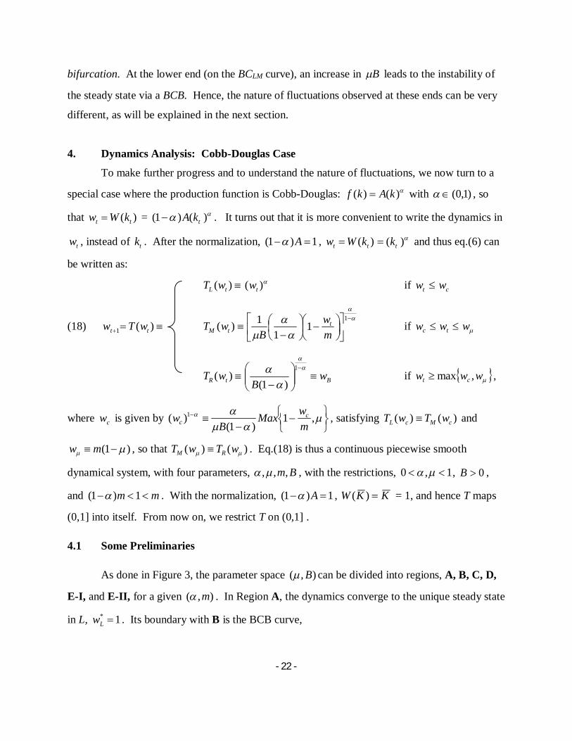
4. Dynamics Analysis: Cobb-Douglas Case

To make further progress and to understand the nature of fluctuations, we now turn to a

special case where the production function is Cobb-Douglas: )()( kAkf with )1,0( , so

that )( tt kWw = )()1( tkA . It turns out that it is more convenient to write the dynamics in

tw , instead of tk . After the normalization, 1)1( A , )( tt kWw )( tk and thus eq.(6) can

be written as:

)( tL wT )( tw if ct ww

(18) )(1 tt wTw )( tM wT

11

11

mw

Bt if www tc

)( tR wT

1

)1(B Bw if www ct ,max ,

where cw is given by

,1

)1()( 1

mwMax

Bw c

c , satisfying )()( cMcL wTwT and

)1( mw , so that )()( wTwT RM . Eq.(18) is thus a continuous piecewise smooth

dynamical system, with four parameters, Bm,,, , with the restrictions, 1,0 , 0B ,

and mm 1)1( . With the normalization, 1)1( A , KKW )( = 1, and hence T maps

(0,1] into itself. From now on, we restrict T on (0,1] .

4.1 Some Preliminaries

As done in Figure 3, the parameter space ),( B can be divided into regions, A, B, C, D,

E-I, and E-II, for a given ),( m . In Region A, the dynamics converge to the unique steady state

in L, 1* Lw . Its boundary with B is the BCB curve,

- 23 -

BCLR :

1

B for m11

on which ** 1 RL ww holds. Its boundary with E-I is the BCB curve,

BCLM:

m

mBCB LM11

1),(

form11

on which ** 1 McL www holds. In Regions B and C, the dynamics converge to the unique

steady state, *Rw , located in R. The outer boundary of C (with D and E) is the BCB curve,

BCMR:

/11)]1([1

mB for m11

on which **RM www holds. In Region D, the unique steady state, *

Mw , located in M, is

locally stable, because 1)('0 * MwT . In Region E, it is locally unstable, because

1)(' * MwT . As we move from D to E, *Mw loses its stability via a flip bifurcation, 1)(' * MwT .

Thus, the boundary between D and E is given by the flip bifurcation curve,

FBM:

/112

])1[(1

),(

mmFBB M for

/11)]1([1

mB .

In Region E, bounded by BCLM (from the left), FBM (from the right) and BCMR (from below), the

unique steady state, *Mw , is unstable, and there exists an absorbing interval, J, whose upper

bound is given by )( cwT . In Region E-I, wwT c )( holds so that only the upward L-branch

and the downward M-branch are involved when T is restricted on )](),([ 2cc wTwTJ , so that:

)( tL wT )( tw for ctc wwwT )(2 (19) )(1 tJt wTw

)( tM wT

11

)1( mw

Bt for )( ctc wTww .

In Region E-II, wwT c )( holds so that all three branches, including the flat R-branch is

involved and )](,[ cB wTwJ . The boundary between E-I and E-II is given by wwT c )( , i.e.,

- 24 -

BCJ:

/11)]1([1

1

mB

between BCLM and FBM.

As already mentioned, the types of fluctuations observed in E-I and E-II are totally

different. In what follows, we will report some results from Sushko, Gardini, and Matsuyama

(2014b; henceforth SGM), which conducts a detailed bifurcation analysis on E-I, particularly on

the nature of transition as we move from D to E-I by crossing the FBM curve or from A to E-I by

crossing the BCLM curve. For the analysis of E-II, as well as the transition between E-I and E-II,

we refer to another companion paper of ours, Sushko, Gardini, and Matsuyama (2014a).

4.2 Crossing the FBM curve: Corridor Stability19

Let us first describe what happens when we move from D to E-I and cross the FBM curve

by decreasing µB. The left panels of Figure 6 and Figure 7 show the graphs of *Mw , cw , )( cwT ,

as well as period-2 cycles, as functions of µB. Also shown are the three critical values of µB:

),( mFBM , at which 1)(' * MwT (the flip bifurcation of *Mw occurring at the boundary

between D and E-I);

),(2 mBC , at which cc wwT )(2 (the existence of the period-2 cycle, )( cc wTw );

),(2 mFB , at which 1)()'( 1 wTT LM , where 1w is given by 11 ))(( wwTT LM (the flip

bifurcation of the period-2 cycle that alternates between the L- and the M-branch,

2121 )()( wwTwTw LM ).20

Figure 6 illustrates the case of α < 0.5, for which ),(2 mBC > ),( mFBM > ),(2 mFB

holds. For µB > ),(2 mBC , the unique steady state, *Mw , is not only stable (as indicated by the

solid line) but also globally attracting. At µB = ),(2 mBC , the period-2 cycle, )( cc wTw , is

born via a fold BCB. On the right panel, this is depicted by the graph of )(2 wT in Red, which

touches the 45º line at cww and )( cwTw . As µB declines further, this period-2 cycle is split

into a pair of period-2 cycles, one stable (as indicated by the pair of the solid lines on the left 19 Much of this section is based on Section 4 of SGM. 20 Some algebra yields ),(2 mFB = /12 /)1()1/( m , where )1/( . Generally,

),(2 mBC can be defined only implicitly.

- 25 -

panel), 2121 )()( wwTwTw LM , alternating between L and M, and one unstable (as indicated

by the dashed curves on the left panel), oscillating within the M-branch.21 For ),( mFBM < B

< ),(2 mBC , the stable steady state, *Mw , co-exists with the stable period-2 cycle. Their basins

of attraction are separated by the unstable period-2 cycle and its pre-images. Then, as µB

continues to decrease and moves toward the boundary with E-I, the unstable period-2 cycle

approaches and merges with the steady state, *Mw , and disappears at the subcritical flip at B =

),( mFBM . On the right panel, this is depicted by the graph of 2T in Blue, which is concave in

),( *Mc ww and convex in ))(,( *

cM wTw for 5.0 with *Mw , the inflection point, being tangent to

the 45º line.22 Upon entering E-I, the steady state *Mw becomes unstable (as indicated by the

dashed line), while the period-2 cycle alternating between M and L, 2121 )()( wwTwTw LM ,

remains stable. This continues, as long as ),( mFBM > B > ),(2 mFB , i.e., until this period-2

cycle loses its stability via a flip bifurcation at B = ),(2 mFB .23

Figure 7 illustrates the case of 5.0 , for which ),( mFBM > ),(2 mBC holds. Figure 7

further assumes ),(2 mBC > ),(2 mFB , which holds for α not too large. As shown on the left

21 As shown on the right panel, )()(2 wTTwT LM is decreasing in cww and )()( 22 wTwT M is increasing in

cww ; )(2 wT has thus a kink at cww . Before this BCB, cc wwT )(2 and, for 5.0 , 2T intersects with the

45º line only at *Mw , so there is no period-2 cycle, hence no cycle of any periodicity. At the BCB, where

cc wwT )(2 , the left derivative of 2T at cw satisfies 1)()'(0 cLM wTT and the right derivative satisfies

1)()'( 2 cM wT . After this BCB, cc wwT )(2 holds, thereby creating two intersections with the 45º line, one below

cw and one above cw . The period-2 cycle alternating between L and M is stable because it corresponds to the first

intersection where the slope of 2T is less than one in absolute value. The period-2 cycle confined with M is unstable, because it corresponds to the second intersection where the slope of 2T is greater than one. 22 Note that, when *

Mw , as the fixed point of T , undergoes a flip bifurcation 1)(' * MwT to create a period-2 cycle

of T , *Mw , as the fixed point of 2T , undergoes a pitchfork bifurcation, 1)()'( *2 MwT , to create a new pair of the

fixed points of 2T , neither of which is a fixed point of T . 23 This last statement, and the left panel of Figure 6, assume )1/(1 2 m so that B = ),(2 mFB >

),( mBCLM , which is necessary for the flip bifurcation of this period-2 cycle to occur in E-I. If )1/(1 2 m , ),(2 mFB < ),( mBCLM , and hence this period 2-cycle never undergoes a flip bifurcation, as B declines. Instead,

it shrinks and converges to 1* Lw and disappears at the BCLM curve. Indeed, we will show later that the period-2

occurs immediately after crossing the BCLM curve from A to E-I under the condition, )1/(1 2 m . See also Figure 10.

- 26 -

panel, the unique steady state, *Mw , is globally attracting in D, i.e., for B > ),( mFBM . Then,

it undergoes a supercritical flip at the boundary with E-I, i.e., at B = ),( mFBM . On the right

panel, this is depicted by the graph of 2T in Blue, which is convex in ),( *Mc ww and concave

in ))(,( *cM wTw for 5.0 with *

Mw , the inflection point, being tangent to the 45º line. As B

< ),( mFBM , the steady state becomes unstable, which creates a stable period-2 cycle. This cycle

oscillates entirely within the M-branch for ),( mFBM > B > ),(2 mBC . Then, at B =

),(2 mBC , this cycle collides with the border with cw . On the right panel, this is depicted by the

graph of )(2 wT in Red, with cc wwT )(2 . When α is not too large and hence ),(2 mBC >

),(2 mFB holds, one can show that the left derivative of 2T at cww is less than one in

absolute value. This ensures that, after the BCB, when 2T intersects with the 45º line

below cww , its slope is less than one in absolute value for ),(2 mBC > B > ),(2 mFB , so

that the period-2 cycle alternating between M and L, 2121 )()( wwTwTw LM , is stable. 24

This cycle then loses its stability at B = ),(2 mFB .25

What happens for the non-generic case of α = 0.5? In this case, the map is linear in the

M-branch. The unique steady state, *Mw , is stable and globally attracting, until B =

),2/1( mFBM = ),2/1(2 mBC = m/1 , where *Mw loses its stability via a degenerate flip, which

creates a continuum of (not asymptotically) stable period-2 cycles, with any point in

)](,(),[ **cMMc wTwww being 2-periodic. For ),2/1( mFBM = ),2/1(2 mBC > B > ),2/1(2 mFB ,

there exists a stable period-2 cycle, alternating between M and L. This becomes unstable at B

= )4/(3),2/1( 22 mmFB .

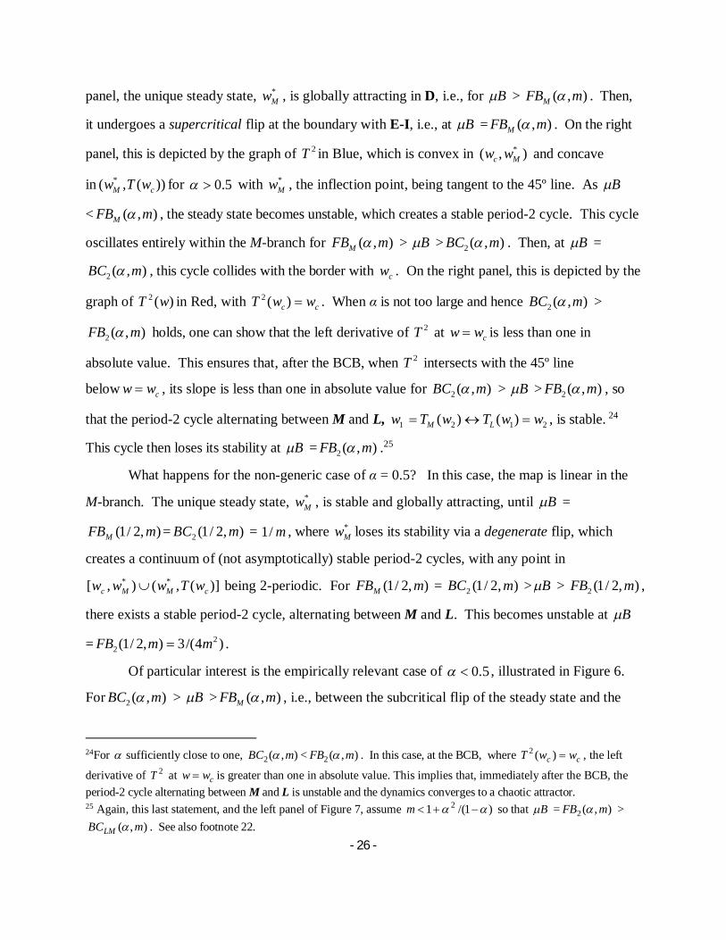
Of particular interest is the empirically relevant case of 5.0 , illustrated in Figure 6.

For ),(2 mBC > B > ),( mFBM , i.e., between the subcritical flip of the steady state and the

24For sufficiently close to one, ),(2 mBC < ),(2 mFB . In this case, at the BCB, where cc wwT )(2 , the left

derivative of 2T at cww is greater than one in absolute value. This implies that, immediately after the BCB, the period-2 cycle alternating between M and L is unstable and the dynamics converges to a chaotic attractor. 25 Again, this last statement, and the left panel of Figure 7, assume )1/(1 2 m so that B = ),(2 mFB >

),( mBCLM . See also footnote 22.

- 27 -

fold BCB, the locally stable steady state co-exists with the locally stable period-2 cycle. And

the basin of attraction of the steady state is bounded by the unstable period-2 points, suggesting

that the steady state possesses the corridor stability a la Leijonhufvud (1973): i.e., it is stable and

self-correcting against small shocks but unstable against large shocks. Furthermore, when a

parameter change causes the steady state to lose its stability via the subcritical flip, its effects are

both catastrophic and irreversible. They are catastrophic in the sense that, when the economy,

initially located in the steady state, becomes dislocated due to the parameter change, it converges

to the period-2 cycle that is far away from the steady state, causing it to fluctuate widely, no

matter how small the parameter change is. In other words, the effects are discontinuous in the

parameter change. Furthermore, these effects are irreversible in the sense that reversing the

parameter to the original value and restoring the stability of the steady state do not allow the

economy to return to the steady state, because the period-2 cycle remains stable. 26 This

suggests, among other things, that even a small, temporary credit crunch shock, captured by a

small, one-time reduction in µ, could have large, permanent effects on the volatility.

Why do smaller values of ensure the corridor stability? In other words, how does the

unique steady state manage to maintain its local stability at least for a while when a decline in

B causes global instability of the dynamical system? The intuition is quite simple. In a

neighborhood of the steady state, *Mw , both the Good and the Bad projects are financed so that

)( twR = )(' 11 tt kfr holds. As a small increase in the net worth tw would allow the agents

running the Bad projects to offer a higher rate of return to the lender, this bids up the equilibrium

rate of return, 1tr , which causes a decline in the capital-labor ratio, 1tk . However, with a small

share of capital in the final goods production, a small decline in 1tk is enough to restore the

equilibrium, which means that the negative effect on 1tw = )( 1tkW is small, which dampens the

effect of a small increase in tw .

4.3 Crossing the BCLM curve27

26For the supercritical case of α > 0.5 (shown in Figure 7), the size of fluctuations along the stable period-2 cycle created by the flip increases continuously with the parameter. Thus, if the parameter change is reversed, the stable cycle shrinks and merges to the steady state, which allows the economy to return to it. 27 Much of this section is based on Section 3 of SGM.

- 28 -

Let us now describe what happens immediately after an increase in B leads to a

transversal crossing of the BCLM curve from A to E-I, which causes 1* Lw to disappear. This

can be done by using the following piecewise linear map:

(20)

01)(01)(

)(1tttR

tttLtt xifbxx

xifaxxxx

,

with

(21) )1,0()('lim1

wTaw

)1,()()1)(1(

)('lim1

mwB

mwTb ,

as an approximation of our map.28 Figure 8a shows the graph of (20), while Figure 8b shows the

graph of the map, (17), to be approximated. The piecewise linear map, (20), is called the skew

tent map, which has been fully characterized. See Sushko, Avrutin, and Gardini (2015) for the

detail. This map has quite rich dynamics. An attracting cycle of any period, as well as a robust

chaotic attractor with any number of intervals, exists for an open region of the parameter space,

(a,b), some of which can be seen in the bifurcation diagram in the ),( ba plane, shown in Figure

9a (with Figure 9b showing an enlargement of its boxed area). In Figure 9a, the colored area

with the number, 2, 3, 4, or 5, is the parameter region for the stable cycle with the number

indicating its periodicity.29 It can be shown that the stable n-cycle visits the downward-sloping

branch only every n-th period, such that 01201 0...)( xxxxx n .30 In both Figures 9a

and 9b, the yellow area, marked as 1Q , represents the parameter region for a chaotic attractor with

one interval. Various white regions in Figure 9b, marked as nnQ 2, or nnQ , (n ≥2), are the regions

of a chaotic attractor with multiple intervals (with the second subscript indicating the number of

28In the language of the dynamical system theory, we use eq.(20) as a normal form for a border collision bifurcation: see Sushko, Avrutin, and Gardini (2015). Intuitively, as we approach BCLM from the interior of E-I, 1cw ,

1)( cwT and 1)(2 cwT , hence, the absorbing interval, )](),([ 2cc wTwTJ , is sufficiently small near the BCLM

curve, which allows us to linearize our map around cw . 29 From the Li-Yorke theorem, we know that there exist an n-cycle for any n ≥ 2 as well as a chaotic trajectory in the parameter region of the stable 3-cycle. However, the stable-3 cycle is a unique attractor in its region, to which the equilibrium trajectory converges from almost all initial conditions. 30 The upper boundary of the region of the stable n-cycle is given by

2

1

)1(1

n

n

aaab . For n ≥ 3, the stable n-cycle

collides with the unstable n-cycle, also existing in the stable region, and disappears via a fold BCB at the upper boundary. The lower boundary of the region of the stable n-cycle is given by nab 1 . The stable n-cycle loses its stability via a degenerate flip bifurcation at this boundary.

- 29 -

intervals). On a chaotic attractor with n intervals, a trajectory visits each interval every n-th

period, but when it returns to the same interval, it never repeats the same value, so that the

trajectory ends up filling each interval. Thus, to naked eyes, the trajectory looks like an n-cycle

with random noises. 31

Using (21), the bifurcation diagram of the skew tent map can be mapped into the

bifurcation diagram in the ),( m plane, as shown in Figure 10. For example, the region of the

stable period-2 cycle for the skew tent map, aabba 1),( , shown in green, is mapped

into 1)1(1),( 2 mm , also shown in green.32 And the region of nnQ 2, is mapped

into the region of nnG 2, , etc. From Figure 10, we can thus find out what happens after the

disappearance of the steady state, 1* Lw , for generic values of ),( m . Note that, for any

)1,0(a and )1,( b , the inverse of (21), a and ])1/[(1 baam , satisfies the

model’s parameter restrictions. Thus, an immediate transition from the stable steady state 1* Lw

to an attracting cycle of any period n ≥ 2, along which the trajectory visits the downward M

branch once every n-th period and then visits the upward L branch for n‒1 consecutive periods,

or to a robust chaotic attractor with any number of intervals can occur upon crossing the BCLM

curve from A to E-I. In particular, in the stability region of cycle of period n ≥ 3 in Figure 10,

the economy converges to an asymmetric cycle, along which n‒1 consecutive periods of gradual

expansion is followed by one period of sharp downturn, for almost all initial conditions in the

neighborhood of the BCLM curve.

The reader might wonder why the periodicity of the stable cycle is higher with a larger α

and a smaller m. With a small m, even a small increase in wt in the downward branch,

31 The first subscript indicates how these chaotic attractors with multiple intervals are born. Starting from the region of the stable n-cycle, a reduction in b causes the n-cycle to lose its stability via a degenerate flip bifurcation, leading to a chaotic attractor with 2n intervals in nnQ 2, . A further reduction in b causes a pairwise merging of these intervals via a merging bifurcation, leading to a chaotic attractor with n intervals in nnQ , . And a further reduction in b causes a sudden expansion of the size of these intervals, via an expansion bifurcation, leading to a chaotic attractor with one interval in 1Q . 32 Notice that one of these conditions for the stable period-2 cycle holds automatically due to the model’s parameter restriction, 1)1( m . The other condition can be rewritten as )1/(1 2 m , so that ),(2 mFB <

),( mBCLM , ruling out the possibility of the flip bifurcation of the period-2 cycle born at the FBM curve . See footnotes 22 and 24.

- 30 -

),1( mwt , causes a sharp increase in the pledgeable rate of return offered by the Bad projects,

and hence a sharp increase in the equilibrium rate of return. In addition, a sharper contraction in

the Good projects is required to compete with a given increase in the equilibrium rate of return

with a larger α. For these reasons, an increase in wt in the downward branch causes a sharper

decline in )( 11 tt kWw with a larger α and a smaller m. Furthermore, a larger α implies more

persistence in the process of capital accumulation, which implies that it takes longer to escape

from the upward branch (i.e., it takes time to build up the net worth to the level that enables the

agents to finance the Bad projects).

4.4 Inside Region E-I33

Having seen what happens in E-I the moment after crossing the BCLM curve, the reader

may wonder what happens as we move away from the BCLM curve and go deeper inside E-I. To

answer this, we have prepared the two bifurcation diagrams, the one in the ),( Bm -plane for α =

1/3 (Figure 11a, with the right panel showing an enlargement of the boxed area on the left panel)

and the other in the ),( B -plane for m = 1.05 (Figure 11b).

For example, for α = 1/3, we know that we can find out what happens immediately after

crossing the BCLM curve and how it depends on m by tracing the vertical line, α = 1/3, in Figure

10. This can be also seen by moving along the BCLM curve on Figure 11a. Likewise, for m =

1.05, we know that we can find out what happens immediately after the BCLM curve and how it

depends on α by tracing the horizontal line, m = 1.05, in Figure 10. This can be also seen by

moving along the BCLM curve on Figure 11b.

Figures 11a and 11b further tell us how these parameter regions of various attractors

extend into the interior of E-I, as B goes up and move away from the BCLM curve. Some of the

boundaries of these regions are marked by the types of bifurcations occurring at these boundaries.

On the right panel of Figure 11a, FBn (n = 2 or 3) denotes the lower boundary of the stable n-

cycle region, where the stable n-cycle loses its stability due to a flip bifurcation; BC2n (n = 2 or

3) denotes the fold BCB related to subcritical FBn; BC3 denotes the upper boundary of the stable

3-cycle region, where the stable 3-cycle disappears due to a fold BCB; Hn (n = 1, 2 or 3) denotes

33 Much of this section is based on Section 5 of SGM.

- 31 -

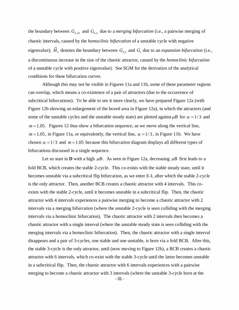
the boundary between nnG 2, and nnG , due to a merging bifurcation (i.e., a pairwise merging of

chaotic intervals, caused by the homoclinic bifurcation of a unstable cycle with negative

eigenvalue); 3~H denotes the boundary between 3,3G and 1G due to an expansion bifurcation (i.e.,

a discontinuous increase in the size of the chaotic attractor, caused by the homoclinic bifurcation

of a unstable cycle with positive eigenvalue). See SGM for the derivation of the analytical

conditions for these bifurcation curves.

Although this may not be visible in Figures 11a and 11b, some of these parameter regions

can overlap, which means a co-existence of a pair of attractors (due to the occurrence of

subcritical bifurcations). To be able to see it more clearly, we have prepared Figure 12a (with

Figure 12b showing an enlargement of the boxed area in Figure 12a), in which the attractors (and

some of the unstable cycles and the unstable steady state) are plotted against B for 3/1 and

05.1m . Figures 12 thus show a bifurcation sequence, as we move along the vertical line,

05.1m , in Figure 11a, or equivalently, the vertical line, 3/1 , in Figure 11b. We have

chosen 3/1 and 05.1m because this bifurcation diagram displays all different types of

bifurcations discussed in a single sequence.

Let us start in D with a high B . As seen in Figure 12a, decreasing B first leads to a

fold BCB, which creates the stable 2-cycle. This co-exists with the stable steady state, until it

becomes unstable via a subcritical flip bifurcation, as we enter E-I, after which the stable 2-cycle

is the only attractor. Then, another BCB creates a chaotic attractor with 4 intervals. This co-

exists with the stable 2-cycle, until it becomes unstable in a subcritical flip. Then, the chaotic

attractor with 4 intervals experiences a pairwise merging to become a chaotic attractor with 2

intervals via a merging bifurcation (where the unstable 2-cycle is seen colliding with the merging

intervals via a homoclinic bifurcation). The chaotic attractor with 2 intervals then becomes a

chaotic attractor with a single interval (where the unstable steady state is seen colliding with the

merging intervals via a homoclinic bifurcation). Then, the chaotic attractor with a single interval

disappears and a pair of 3-cycles, one stable and one unstable, is born via a fold BCB. After this,

the stable 3-cycle is the only attractor, until (now moving to Figure 12b), a BCB creates a chaotic

attractor with 6 intervals, which co-exist with the stable 3-cycle until the latter becomes unstable

in a subcritical flip. Then, the chaotic attractor with 6 intervals experiences with a pairwise

merging to become a chaotic attractor with 3 intervals (where the unstable 3-cycle born at the

- 32 -

subcritical flip is seen colliding with the merging intervals via a homoclinic bifurcation). Then,

the chaotic attractor with 3 intervals experiences a discontinuous increase in its size via an

expansion bifurcation to become a chaotic attractor with one interval (where the unstable 3-cycle

born at a fold BCB is seen colliding with the chaotic attractor via a homoclinic bifurcation).

After this, the chaotic attractor with one interval is the unique attractor, which continuously

shrinks its size and disappears upon entering Region A. We summarize this bifurcation sequence

schematically as follows:

*1

~

3,36,36,312,24,24,2**

3336312242

},3{3},2{2}2,{ L

BCHHFBBCBCHHFBBCFB

M

BC

M wGGGGGGGGwwLMM

.

Finally, let us end our discussion of the interior of E-I region with some numerical plots

of the equilibrium trajectories to see what happens during the transient phase (Figures 13). Again,

we have set 3/1 and 05.1m and chosen values of B from each of the parameter regions

discussed above. Although we have chosen the initial condition fairly close to its attractor, these

plots show that the convergence to the attractor is not immediate. Indeed, this model is capable

of generating quite irregular fluctuations during the transient phase even in the parameter regions

of stable cycles. For example, Figure 13e shows the case where the equilibrium trajectory

asymptotically converges to a stable 3-cycle. This plot shows that during the transient phase, the

equilibrium trajectory looks more like an irregular 6-cycle, and to the naked eye, it is hardly

distinguishable from the case of chaotic attractors with 6 intervals, illustrated in Figure 13f. Yet,

the asymmetry of fluctuations, the patterns of “up”, “up,” “down,” “up”, “up,” and “down,” can

be seen clearly, which is what one should expect from our result in Section 4.3 that, upon

crossing the BCLM curve, the economy experiences two periods of expansion followed by one

period of downturn along its only stable 3-cycle.

5. Concluding Remarks

This paper studied a dynamic general equilibrium model with financial frictions, in which

the economy fluctuates endogenously along its unique equilibrium trajectory. What generates

fluctuations is the changing composition of credit flows across heterogeneous investment

projects, which we call the Good and the Bad. The Good require the inputs supplied by others.

By generating demand for them, they improve net worth of other borrowers. The Bad are

- 33 -

independently profitable, so that they generate less demand spillovers than the Good.

Furthermore, the Bad are subject to the borrowing constraint so that the agents need to have a

high level of net worth to be able to initiate the Bad projects. When the net worth is low, the

agents cannot finance the Bad, and all the credit goes to the Good, even when the Bad are more

profitable than the Good. This over-investment to the Good creates a boom, leading to an

improved net worth. The agents are now able to invest into the Bad. This shift in the

composition of the credit from the Good to the Bad at the peak of the boom causes a decline in

net worth. The whole process repeats itself. Endogenous fluctuations occur because the Good

breed the Bad and the Bad destroy the Good. Such instability and persistent volatility occur

when the following two conditions hold. First, the Bad projects need to be highly profitable so

that the agents are always eager to run them. Second, the Bad projects come with an

intermediate degree of pledgeability, so that the agents cannot finance them when their net worth

are low, but they can when their net worth are high. This implies, among other things, that an

improvement in the financial system could lead to more volatility.

Although this mechanism was already discussed in Matsuyama (2013, Section 2-4),

many additional ingredients of the model, which were introduced to demonstrate the robustness

of the mechanism and to clarify the assumptions that are essential from those that are merely

simplifying, had unfortunately ended up obscuring the mechanism. In this paper, we have shown

that the same dynamical system that governs the equilibrium trajectory can be obtained by a

much simpler setting, which should help to highlight the mechanism through which financial

frictions cause instability and persistent fluctuations. It should also help to make this model

more useful as a building block for future research.

Furthermore, we discussed in greater detail the nature of fluctuations observed for the

case where the production of the final good is Cobb-Douglas. For example, the unique steady

state possesses the corridor stability, which means that it is locally stable but globally unstable.

This also suggests that, when a parameter change causes its local stability, the effects are

catastrophic and irreversible. Furthermore, the dynamics may be characterized by an immediate

transition from the stable steady state to a stable asymmetric cycle of period n ≥ 3, along which n

‒1 ≥ 2 consecutive periods of gradual expansion is followed by one period of sharp downturn, or

by an immediate transition to robust chaotic attractors. We are able to show these results thanks

- 34 -

to recent advances in the theory of piecewise smooth (i.e., regime-switching) dynamical systems,

which have many properties that are quite distinct from and much simpler than those defined by

smooth dynamical systems. In particular, we demonstrated how the skew-tent map provides a

powerful tool for characterizing a regime-switching system. Although a rigorous presentation of

these tools was well beyond the scope of this paper, we have strived to make it accessible to the

economics audience. We hope that our non-technical, heuristic exposition, and “cookbook”

presentation of how to use it, written in the economist-friendly language, serves as an

introduction to this branch of mathematics, which should provide powerful tools for analyzing

regime-switching nonlinear dynamic economic models.

- 35 -

References: Aghion, Philippe, Abhijit Banerjee, Thomas Piketty, “Dualism and Macroeconomic Volatility,” Quarterly

Journal of Economics, 1999, 114 (4), 1359-1397. Avrutin, Viktor, Laura Gardini, Michael Schanz, Iryna Sushko, Fabio Tramontana, Continuous and

Discontinuous Piecewise-Smooth One-Dimensional Maps: Invariant Sets and Bifurcation Structure, World Scientific, 2016 (in progress).

Azariadis, Costas, and Bruce D. Smith, “Financial Intermediation and Regime Switching in Business Cycles,” American Economic Review, 1998, 88(3), 516-536

Baumol, William J., and Jess Benhabib, “Chaos: Significance, Mechanism, and Economic Applications,” Journal of Economic Perspectives, 3 (Winter 1989): 77-105.

Benhabib, Jess, and Miyao, Takahiro, “Some New Results on the Dynamics of the Generalized Tobin Model,” International Economic Review, 22 (October 1981): 589-596.

Bernanke, Ben, and Mark Gertler, “Agency Costs, Net Worth, and Business Fluctuations,” American Economic Review, 79, March 1989, 14-31.

Diamond, Peter, “Government Debt in a Neoclassical Growth Model,” American Economic Review, December 1965, 55, 1126-1150.

Favara, Giovanni, “Agency Problems and Endogenous Investment Fluctuations,” Review of Financial Studies, 2012, 25 (7), 2301-2342.

Figueroa, Nicolás, and Oksana Leukhina, “Liquidity and Credit Cycles,” University of Washington Working Paper, September 2013.

Gardini, Laura, Iryna Sushko, and Ahmad K. Naimzada, “Growing Through Chaotic Intervals,” Journal of Economic Theory, 143, 2008, 541-557.

Kindleberger, Charles P., Manias, Panics, and Crashes: A History of Financial Crises, The Third Edition, New York, John Wiley & Sons, Inc., 1996.

Kiyotaki, Nobuhiro, and John H. Moore, “Credit Cycles,” “Journal of Political Economy, 105, April 1997, 211-248.

Leijonhufvud, Axel, “Effective Demand Failures,” Swedish Journal of Economics, March 1973, 27-48. Martin, Alberto, “Endogenous Credit Cycles,” CREI and Universitat Pompeu Fabra Working Paper, 2008. Matsuyama, Kiminori, “Growing Through Cycles,” Econometrica, 67, March 1999, 335-347. Matsuyama, Kiminori, “Credit Traps and Credit Cycles,” American Economic Review, 97, March

2007,503-516. Matsuyama, Kiminori, “Aggregate Implications of Credit Market Imperfections,” in D. Acemoglu, K.

Rogoff, and M. Woodford, eds., NBER Macroeconomics Annual 2007, vol. 22, University of Chicago Press, 2008, 1-60.

Matsuyama, Kiminori, “The Good, The Bad, and The Ugly: An Inquiry into the Causes and Nature of Credit Cycles,” Theoretical Economics 8, 2013, 623-651.

Mendoza, Enrique G., and Marco E. Terrones, 2008, “An Anatomy of Credit Booms: Evidence from Macro Aggregates and Micro Data,” NBER Working Paper, 14049.

Minsky, Hyman P., “The Financial Instability Hypothesis: Capitalistic Processes and the Behavior of the Economy,” in C.P. Kindleberger and J.P. Laffargue, eds., Financial Crises: Theory, History, and Policy (Cambridge, Cambridge University Press, 1982); 13-29.

Myerson, Roger B., “A Model of Moral Hazard Credit Cycles,” Journal of Political Economy, 105, October 2012, 847-878.

Myerson, Roger B., “Moral-Hazard Credit Cycles with Risk-Averse Agents,” Journal of Economic Theory, 153, September 2014, 74-102.

Reichlin, Pietro, and Paolo Siconolfi, “Optimal Debt Contracts and Moral Hazard along the Business Cycle,” Economic Theory, 24, 2004, 75-109.

- 36 -

Schularick, Moritz, and Alan M. Taylor, “Credit Booms Gone Bust: Monetary Policy, Leverage Cycles, and Financial Crises, 1870-2008,” American Economic Review, 102 (2), 1029-61.

Sushko, Iryna, Viktor Avrutin, and Laura Gardini, “Bifurcation Structure in the Skew Tent Map and Its Application As a Border Collision Normal Form,” Journal of Difference Equations and Applications, December 2015, 1-48.

Sushko, Iryna, Laura Gardini, and Kiminori Matsuyama, “Superstable Credit Cycles and U-sequence,” Chaos, Solitons, Fractals, 59, February 2014a, 13-27.

Sushko, Iryna, Laura Gardini, and Kiminori Matsuyama, “Chaos in a Model of Credit Cycles with Good and Bad Projects,” WP-EMS #2014/05, University of Urbino, downloadable at http://www.econ.uniurb.it/RePEc/urb/wpaper/WP_14_05.pdf , 2014b

Tirole, Jean, The Theory of Corporate Finance, Princeton University Press, Princeton, 2005.

- 37 -

O kt

W(kt)

kt+1

kB

)()'( 1 BfwB

Figure 1: Non Distortionary Case: Bwf )(' )()( BB kWwkWw a) All credit flows into the Good for )()( BBtt kWwkWw , i.e., Bwf t )(' . All additional

credit flows into the Bad for )()( BBtt kWwkWw . Hence, Bc kk . b): The map has two branches with one kink at Bk : upward on the Left and flat on the Right

wB

B

O wt

µB

f'(wt) R(wt)

wµ

- 38 -

O kt

W(kt)

kt+1

kc

W(kc)

kµ

W(kB)

kB

Figure 2: Distortionary Case: Bwf )(' )()( BB kWwkWw a) All the credit continues flowing into the Good, even after Bwf t )(' , implying

ccBB wkWkWw )()( . After cctt wkWkWw )()( , the credit is diverted away from the Good to the Bad, until wkWkWw tt )()( , after which only additional credit flows into the Bad.

b): The map has three branches with two kinks, ck < k : upward on the left ( tk < ck ), downward in the middle ( ck < tk < k ), and flat on the right ( tk > k ). Over-Investment of the Good for ( Bk < tk < k ).

wµ

B

O wt

µB

f'(wt) R(wt)

wc wB

- 39 -

µ O 1

B

A

A B

C

D

E-I

Endogenous Fluctuations

(Locally)Oscillatory Convergence

mK /1

E-II

)(' Kf

))1((' mfB

)))1(((' 1 mWfB

mmWmWfB ))1((1))1((('

11

mKKfB 1)('

mmfWmffB ))((1))(('

11

LRBC

MRBC LMBC

JBC

MFB

Figure 3: Parameter Configuration: )()( KfmKWK . Assumption (A2), mK , ensures the existence of region A above the horizontal line, )(' KfB . The parameter restriction, )(Kfm , ensures the existence of region E. The boundaries between A and B ( LRBC ), between B and C, between C and D/E-II ( MRBC ), between E-I and E-II ( JBC ) and between E-I and A ( LMBC ) are all issuing from the point, ))(',/1(),( KfmKB . The boundaries between B and C, between C and D ( MRBC ) and between E-I and E-II ( JBC ) are all asymptotic to 1 . The boundaries between D and E ( MFB ) and between E-I and A ( LMBC ) are hyperbolae and asymptotic to 0 .

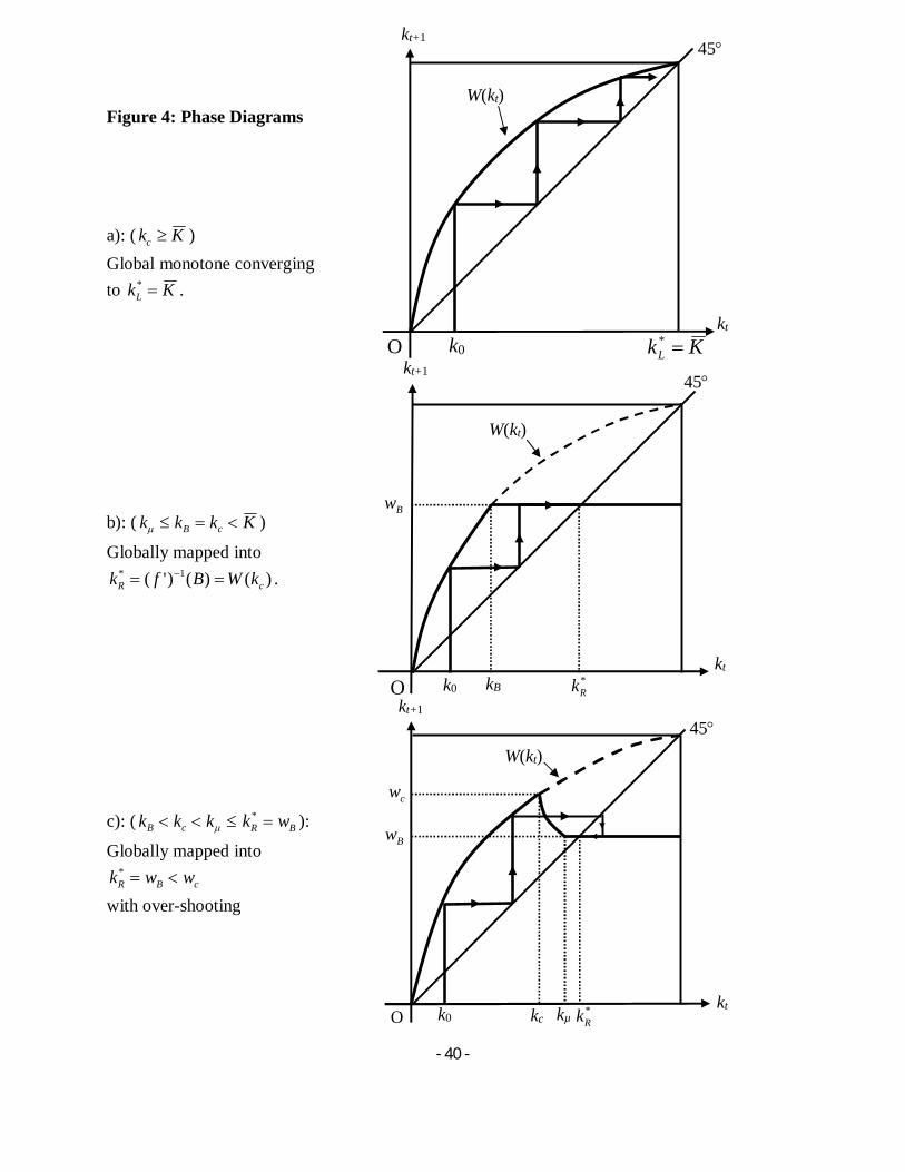
- 40 -

Figure 4: Phase Diagrams

a): ( Kkc ) Global monotone converging to KkL

* .

b): ( Kkkk cB )

Globally mapped into )()()'( 1*

cR kWBfk . c): ( kkk cB BR wk * ):

Globally mapped into

cBR wwk * with over-shooting

O kt

45

W(kt)

k0

kt+1

KkL *

kt

45 W(kt)

k0

kt+1

*Rkkc

cw

Bw

kµ O

Bw

O kt

45

W(kt)

k0

kt+1

*RkkB

- 41 -

Figure 4: Phase Diagrams (Continue…) d): ( kkk Mc * ) (Locally) oscillatory convergence to *

Mk . e): ( kkk Mc * ) Endogenous fluctuations with the unstable steady state, *

Mk . Depending on whether the absorbing interval, J, includes the flat branch, E-I: Only two branches (L and M) are involved in J. E-II: All three branches (L, M, and R) are involved in J, as shown here.

O kt

45

W(kt)

k0

kt+1

*Mk*

kc

cw

Bw

kµ

O kt

45

W(kt)

k0

kt+1

*Mk

kc

cw

kµ Bw

J

J

Bw

cw

- 42 -

Figure 5a: Map restricted on the Absorbing Interval, J, above BCJ.

Figure 5b: Parameter Configuration in (m, µB) above BCJ.

kt

45

W(kt)

kt+1

*Mk

kc

cw

J

J

cw)( cM w

m 0

µB

A

D

E-I

)(Kf K

mmfWmffB ))((1))(('

11

mKKfB 1)('

)(1)('

KfKKf

:MFB

:LMBC

- 43 -

Figure 6: Crossing the FBM Curve for α < 0.5: Subcritical FB and Fold BCB

Figure 7: Crossing the FBM Curve for α > 0.5: Supercritical FB and Persistence BCB

45

*Mwcw )( cwT

subcritical FB

fold BCB

45

*Mw

cw )( cwT

persistence BCB

supercritical FB *Mw

cw

)( cwT

supercritical flip bif.

persistence BCB

B),(2 mBC ),( mFBM ),(2 mFB

E-I D

M

L

)( 12 wTw L

)( 21 wTw M

*Mw

cw

)( cwT

subcritical flip bif.

fold BCB

B),(2 mBC ),( mFBM ),(2 mFB

M

L

Corridor Stability

E-I D

)( 12 wTw L

)( 21 wTw M

- 44 -

Figure 8:

a) Skew Tent Map ( 10 a ; 1b ) b) Eq. (19) after crossing the BCLM curve

Figure 9: Bifurcation Diagrams for Skew Tent Map:

a) b)

In Figure 9a), the numbers, 2, 3, 4, and 5, in the colored regions indicate the periodicity of stable cycles. The yellow region, Q1 , indicates the region of a chaotic attractor with one interval. A magnification of the boxed area in 9a) is shown in Figure 9b). The white regions indicate the regions of a chaotic attractor with multiple intervals, with the second subscript indicates the number of intervals. See Sushko, Avrutin, and Gardini (2015) for more detail.

45

)(2cwT

wt

45 wt+1

cw

)( cwT

xt

45 xt+1

b1 1

1

)1(1 ba

- 45 -

Figure 10: Bifurcation diagram for Eq. (19) upon Crossing the BCLM curve

This bifurcation diagram is obtained from the bifurcation diagram of the skew-tent map (see Figure 9), by using eq.(21). The number, 2, 3, and 4, in the colored areas indicate the periodicity of stable cycles. The yellow region with G1 indicates a chaotic attractor with one interval. The white regions indicate a chaotic attractor with multiple intervals (the second subscript indicates the number of intervals). With 1b , the Red region for the skew tent map (the region of stable steady state) seen in Figure 9a) would map into Gray in this figure, which is outside of our parameter range.

- 46 -

Figure 11: Two Bifurcation Diagrams for Eq.(19): Inside Region E-I

a) ),( Bm -plane with 3/1

b) ),( B -plane with 05.1m

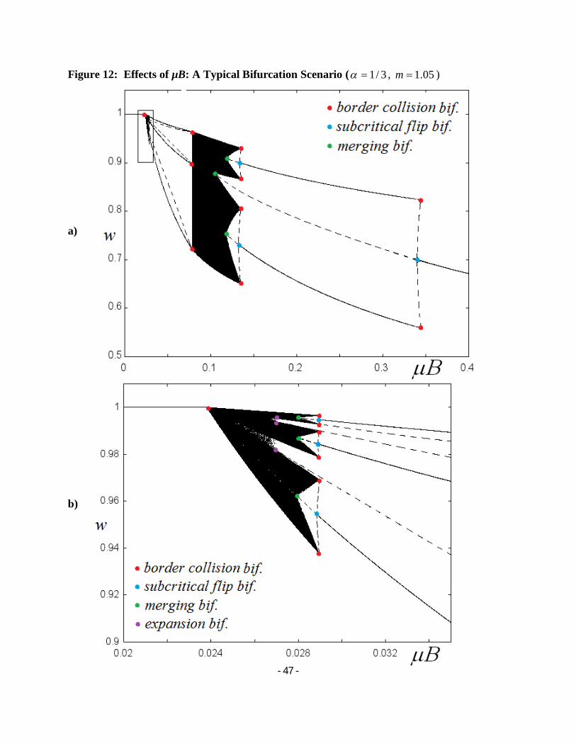
- 47 -

Figure 12: Effects of µB: A Typical Bifurcation Scenario ( 3/1 , 05.1m ) a) b)

- 48 -

Figure 13: Some Trajectories ( 3/1 , 05.1m )

a) µB=0.2 (2-cycle), with w0 = 0.9.

b) µB = 0.125 (G2,4), with w0 = 0.9. c)

- 49 -

µB = 0.1125 (G2,2), with w0 = 0.9.

d) µB = 0.085 (G1), with w0 = 0.9.

e)

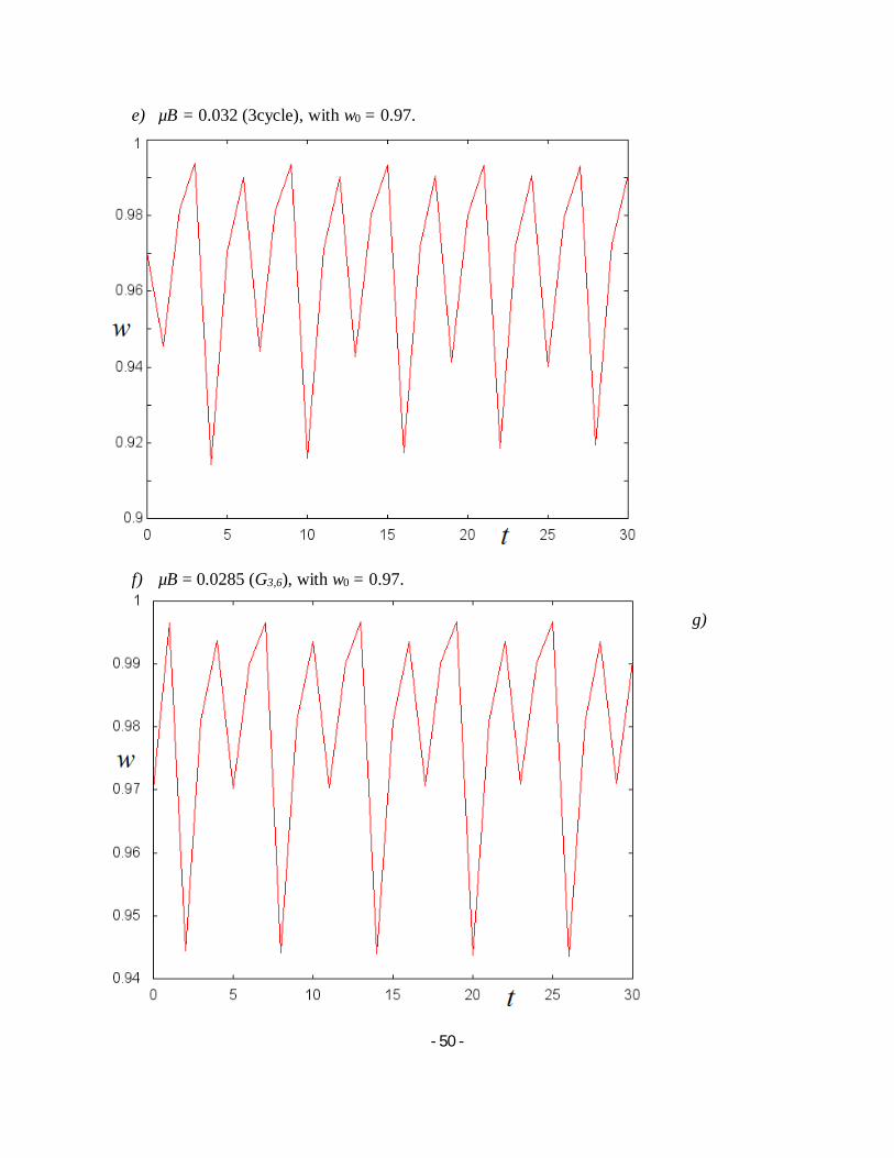
- 50 -

e) µB = 0.032 (3cycle), with w0 = 0.97.

f) µB = 0.0285 (G3,6), with w0 = 0.97.

g)

- 51 -

g) µB = 0.0275 (G3,3), with w0 = 0.97.

h) µB = 0.0245 (G1), with w0 = 0.99.