revised spring creek awwtp cso disinfection ... spring creek awwtp cso disinfection demonstration...

Revised Spring Creek AWWTP CSO Disinfection Demonstration Study

December 2015

The City of New York

Department of Environmental Protection

Bureau of Wastewater Treatment


i

TABLE OF CONTENTS

I. INTRODUCTION ................................................................................................................ 1

II. EXISTING CONDITIONS ..................................................................................................... 1

III. DESIGN CRITERIA............................................................................................................. 2

IV. DESIGN & CONSTRUCTION SCOPE OF WORK.................................................................... 7

V. PROJECT SCHEDULE........................................................................................................ 7

VI. DEMONSTRATION TESTING SCOPE OF WORK................................................................... 7

LIST OF FIGURES

Figure 1 - Process Spring Creek Flow Schematic……………………………………………………………....3

Figure 2 - Spring Creek Flow Diagram……………………………………………………………………….…..4

Figure 3 - Spring Creek 5 Minute Wet Weather Flows..…………………………………………………….….5

Figure 4 - Schematic of the Existing Hypochlorite System………………………………………………..…...6

Figure 5 - CSO Demonstration Facility Schedule……….……………………………………………….……...7

Figure 6 - Spring Creek Sampling Locations……………………………………………………….……………9


Resubmittal: December 2015 1

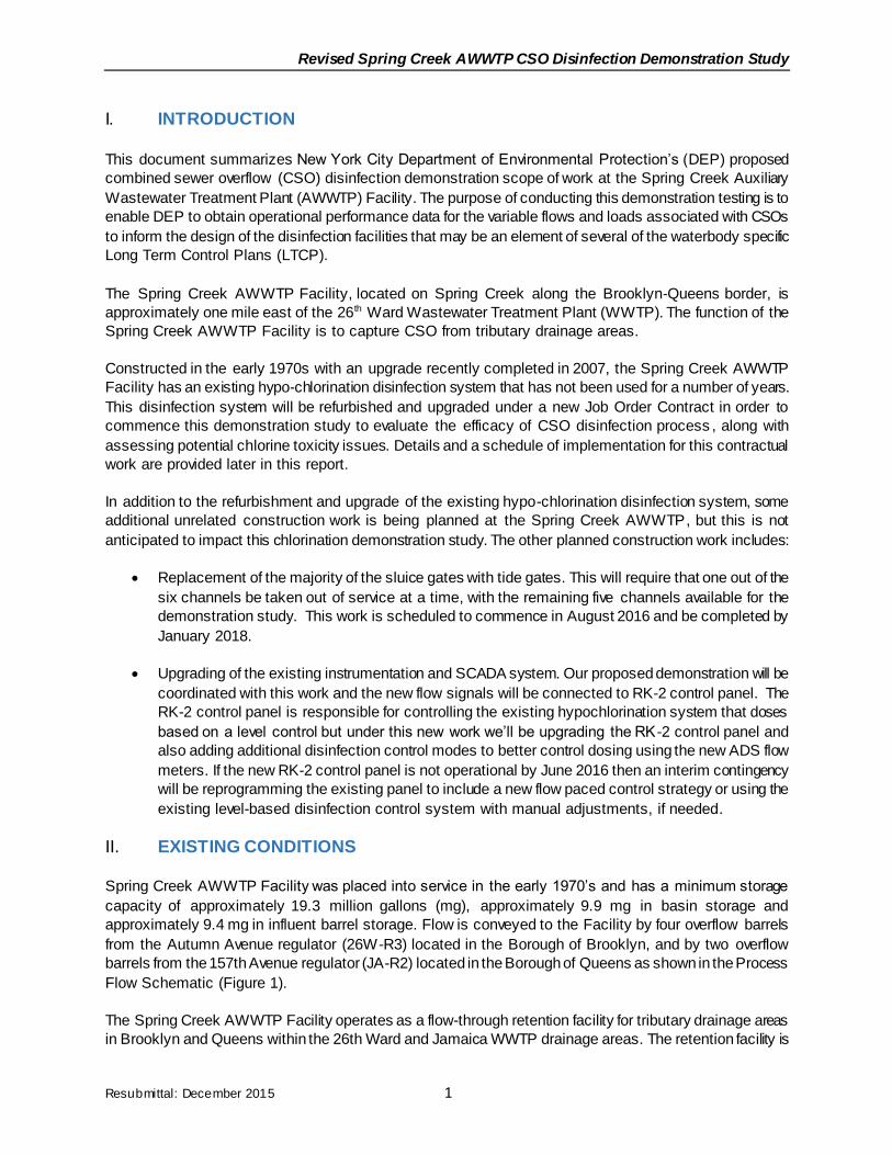
I. INTRODUCTION

This document summarizes New York City Department of Environmental Protection’s (DEP) proposed

combined sewer overflow (CSO) disinfection demonstration scope of work at the Spring Creek Auxiliary

Wastewater Treatment Plant (AWWTP) Facility. The purpose of conducting this demonstration testing is to

enable DEP to obtain operational performance data for the variable flows and loads associated with CSOs

to inform the design of the disinfection facilities that may be an element of several of the waterbody specific

Long Term Control Plans (LTCP).

The Spring Creek AWWTP Facility, located on Spring Creek along the Brooklyn-Queens border, is

approximately one mile east of the 26th Ward Wastewater Treatment Plant (WWTP). The function of the

Spring Creek AWWTP Facility is to capture CSO from tributary drainage areas.

Constructed in the early 1970s with an upgrade recently completed in 2007, the Spring Creek AWWTP

Facility has an existing hypo-chlorination disinfection system that has not been used for a number of years.

This disinfection system will be refurbished and upgraded under a new Job Order Contract in order to

commence this demonstration study to evaluate the efficacy of CSO disinfection process , along with

assessing potential chlorine toxicity issues. Details and a schedule of implementation for this contractual

work are provided later in this report.

In addition to the refurbishment and upgrade of the existing hypo-chlorination disinfection system, some

additional unrelated construction work is being planned at the Spring Creek AWWTP, but this is not

anticipated to impact this chlorination demonstration study. The other planned construction work includes:

Replacement of the majority of the sluice gates with tide gates. This will require that one out of the

six channels be taken out of service at a time, with the remaining five channels available for the

demonstration study. This work is scheduled to commence in August 2016 and be completed by

January 2018.

Upgrading of the existing instrumentation and SCADA system. Our proposed demonstration will be

coordinated with this work and the new flow signals will be connected to RK-2 control panel. The

RK-2 control panel is responsible for controlling the existing hypochlorination system that doses

based on a level control but under this new work we’ll be upgrading the RK -2 control panel and

also adding additional disinfection control modes to better control dosing using the new ADS flow

meters. If the new RK-2 control panel is not operational by June 2016 then an interim contingency

will be reprogramming the existing panel to include a new flow paced control strategy or using the

existing level-based disinfection control system with manual adjustments, if needed.

II. EXISTING CONDITIONS

Spring Creek AWWTP Facility was placed into service in the early 1970’s and has a minimum storage

capacity of approximately 19.3 million gallons (mg), approximately 9.9 mg in basin storage and

approximately 9.4 mg in influent barrel storage. Flow is conveyed to the Facility by four overflow barrels

from the Autumn Avenue regulator (26W-R3) located in the Borough of Brooklyn, and by two overflow

barrels from the 157th Avenue regulator (JA-R2) located in the Borough of Queens as shown in the Process

Flow Schematic (Figure 1).

The Spring Creek AWWTP Facility operates as a flow-through retention facility for tributary drainage areas

in Brooklyn and Queens within the 26th Ward and Jamaica WWTP drainage areas. The retention facility is



designed to fully contain certain storms and act as a flow-through facility to maximize the reduction of CSO

overflows to Spring Creek during larger storms. The total tributary area is composed of 3,256 acres, of

which 1,874 acres are in Brooklyn and 1,382 acres are in Queens.

The CSO is conveyed to Spring Creek basins by four overflow barrels from the Autumn Avenue regulator

(26W-R3) and two overflow barrels from the 157th Avenue regulator.

The control of influent flow to the Spring Creek AWWTP Facility is accomplished through automated control

of the Autumn Avenue Regulator (26W-R3) and from overflow from the 157th Avenue Regulator (JA-R2),

The Facility has six basins with a minimum retention volume, including inline storage, of 19.3 mg. Drain-

back from the Facility is by gravity to elevation -7.50 (Brooklyn Highway Datum) and by pumping below this

level. Approximately 7.0 mg of CSO is stored in the basins above elevation –7.50 and approximately 8.9

mg are stored above elevation -7.5 in the influent barrels. The stored volume flows by gravity back to the

collection system through 26W-R3 influent barrels. A schematic and flow diagram of the existing facility is

shown on Figures 1 and Figures 2.

The original disinfection control strategy was semi-automated using the level sensors within the basins but

also relied on the operators to manually sample the influent chlorine residual and then adjust the

hypochlorite metering pumps accordingly. The neat hypo is pumped into a common pipe with water from

the head end of the creek that is used for carrier water. The diluted hypochlorite is added via a diffuser grid

into the six channels feeding the basins upstream of the CSO Tank. Some of the hypochlorite piping and

diffusers grids are in need of repair but the metering pumps are in operating condition.

III. DESIGN CRITERIA

Based on work performed by DEP during a CSO disinfection pilot study for the Spring Creek AWWTP

Facility in the 1990’s, the chlorine dosages ranged from 9 to 20 mg/L to achieve a 3 to 4 log. However, the

current goal for CSO disinfection, as outlined in certain LTCPs submitted to DEC for review, is to balance

influent chlorine dosage with potential effluent toxicity due to total residual chlorine (TRC). Therefore, a 2

log targeted reduction of fecal coliform will be the goal of this demonstration test. Based on the pilot study

from the 1990’s, it is anticipated that the required chlorine dosage of about 10 to 15 mg/L and some

subsequent bench scale testing will be done to verify the required dosing range. The projected 5 minute

CSO inflows to the tank based on CY2014 InfoWorks model are provided in Figure 2.

Based on projected InfoWorks CSO influent flow rates as shown on Figure 3 and the typical CSO TRC

dosages, the following hypochlorite flow rates have been calculated assuming a 15 percent hypochlorite

solution:

Table 1 – Projected Hypo Chlorite Dosages

Percentile 5 ppm 10 ppm 15 ppm

Projected Hypo Flow Rate (gph)

90th 230 450 680

10th 5 10 15



Figure 1 - Spring Creek Schematic



Figure 2 - Spring Creek Flow Diagram



The current disinfection system has three existing low range hypochlorite metering pumps rated for flow

rates from 100 to 938 gph based on selected stroke length and have a rated turn down capacity of 10:1

for each pump based on pump speed controls. Based on the projected hypochlorite flow rates from Table

1, the low range metering pumps are properly sized to handle the majority of the CSO events. There is

also sufficient hypochlorite storage capacity using the two existing 12,000 gallon sodium hypochlorite

chemical storage tanks. A schematic of the existing hypochlorite system is provided in Figure 4.

Figure 3 - InfoWorks Projected CSO Flows



Figure 4 - Schematic of Hypochlorite System



IV. DESIGN & CONSTRUCTION SCOPE OF WORK

The proposed design and construction scope of work includes the installation of three new triton influent

flow meters just upstream of the hypochlorite diffusers to monitor flow. This will require running power to

the six new flow meters using the existing conduits where possible, along with some trench work and

installation of new conduit and wire. In addition, a signal wire will need to be run from the flow meters to a

centralized location in the hypochlorite room where the flow signals will be connected to the RK-2 control

panel that is currently the control panel for existing hypochlorite system. The RK-2 control panel is also

being upgraded under a separate contract and included in this scope of work will be programming some

additional TRC automated control strategies using the new ADS flow meters. The hypochlorite pumps and

will provide the ability to run the system either automatically or manually. DEP intends to retain the services

of an outside vendor to maintain the flow meters during the startup and demonstration testing, both to

calibrate and to maintain the system. Additional details on the flow metering equipment and installation are

provided in Attachment 1. Provisions will also be included to tie this local control panel into the remote

SCADA system in the future, so that these newly installed flow meters are used to report CSO overflow

volumes and frequency in the monthly operating reports. In addition to the new flow metering and controls,

some work will be necessary to refurbish some of the hypochlorite piping and hypochlorite diffuser grids

prior to re-commissioning the disinfection system.

V. PROJECT SCHEDULE

Figure 5 provides the schedule for placing the CSO demonstration facility on-line and performing the

demonstration testing.

Figure 5. CSO Demonstration Facility Schedule

VI. DEMONSTRATION TESTING SCOPE OF WORK

DEP personnel will coordinate with the City College of New York (CCNY) staff about impending events to

enable necessary mobilization. CCNY will go to the facility to collect and analyze samples prior to rain

events that are projected to occur during the daytime hours, no manual night sampling is planned. A

schematic showing the sampling locations is provided in Figure 6, with the following overview of the

proposed sampling plan:

Pre-chlorinated influent samples will be collected prior to hypo addition and the samples will be

analyzed for fecal coliform and enterococcus. CCNY has obtained NELAP certification for fecal

May Jun Jul Aug Sep Oct Nov Dec Jan Feb Mar Apr May Jun Jul Aug Sep Oct Nov Dec Jan Feb Mar Apr May Jun

Design Completion

Job Order Issued

Substantial Completion

Startup & Testing

Construction Completion

Demonstration Testing

CY2015 CY2016 CY2017



coliform and enterococcus and will be using standard methods approved methodologies for the

analysis as shown in Attachment 2.

Chlorinated influent samples will be collected just downstream of the hypochlorite diffuser and

analyzed for fecal coliform, enterococcus and TRC.

There are limited access locations to collect samples from the middle of the tank, so a duplicate

chlorinated influent sample collected will be held for fixed durations to mimic detention time in the

tank, and then re-analyzed for fecal coliform, enterococcus, and TRC.

It is not anticipated that the tank will frequently overflow; however, when it does, overflow samples

will be collected and analyzed for fecal coliform, enterococcus, and TRC.

During overflow events, manual samples will also be collected of the ambient water from the dilution

water wet well from which water from the head end of Spring Creek is pumped into the hypochlorite

feed lines to be used as carrier water to convey hypochlorite into the two hypochlorite diffusion

chambers. A schematic of the dilution water system is provided in Attachment 3 and it is in a

separate chamber from the disinfected CSO overflow and is open to the creek therefore

representative of ambient conditions.

In addition to these ambient grab samples, DEP will be conducting a controlled, bench-top chlorine

degradation analysis using different predetermined doses of chlorine, adding it to a raw CSO

sample, simulating detention time of the CSO tank, and then dosing it to a fixed volume of Jamaica

Bay water and measuring the observed TRC residuals A detailed description of the bench scale

ambient TRC decay studies in included in Attachment 3 along with some additional details on

ambient sampling location.

Below is a summary of the proposed analytical methods to be used. Samples will be analyzed on site and

at the City College Laboratory for analysis. A schematic with the sampling locations is provided on Figure

6.

Methods for Analysis

Analyte CCNY method Note

Coliform,

Fecal HACH Method 8074 EPA 9222 D

Enterococci Method 1600 EPA 821-R-09-016

TRC D1253-08



Figure 6. Spring Creek AWWTP Sampling Locations

Current Location of Auto sampler

Proposed Sampling Locations

Attachment 1

ADS Flow Meters

H A R D W A R E

This multiple technology flow monitor will power almost every available sensor technology that is used in wastewater applica-tions today. It is the most versatile and cost-effective, multiple-technology flow monitor on the market. The TRITON+ includes three multiple technology sensor options: a Peak Combo Sensor, a Surface Combo Sensor, and an Ultrasonic Level Sensor (see inside for technology and specifications). This array of monitoring tech-nologies provides for unmatched flexibility in a fully integrated, fit-for-purpose monitoring platform.

The TRITON+ platform adapts to a wide range of customer applica-tions and budgets. It can be configured as an economical single sensor monitor or dual sensor monitor. It offers a longer battery life and fewer parts for a more reliable system. This provides a low-er purchase price and a lower ownership cost over the life of the monitor. The TRITON+ has the lowest operational cost per data sample of any Intrinsically Safe flow monitor available.

ADS TRITON+

The new ADS TRITON+™ is a “Fit-for-Purpose” open channel flow monitor for use in sanitary, combined, and storm sewers. It is designed to be the most versatile flow monitoring system available for wastewater collection applications. It supports single pipe or dual pipe flow measurement installations and is certified to the highest level of Intrinsic Safety.

TRITON+ Features

About

A leading technology

and service provider, ADS

Environmental Services®

has established the industry

standard for open channel flow

monitoring and has the only

ETV-verified flow monitoring

technology for wastewater

collection systems. These

battery-powered monitors are

specially designed to operate

with reliability, durability, and

accuracy in sewer environments.

A Division of ADS LLC

• Versatile performance that is easy to install and operate

• Two sensor ports supporting 3 interchangeable sensors providing up to 6 sensor readings at a time

• Single or dual pipe/monitoring point measurement capabilities

• Multi-carrier cellular or serial communication to help optimize coverage and cost

• Industry-leading battery life with a 3G/4G UMTS/HSPA+ wireless connection providing up to 15 months at the standard 15-minute sample rate (varies with sensor configuration)

• External power and Modbus network connectivity option available with an ADS External Power and Communications Unit (ExPAC) and a 9-36 VDC power supply

• Analog and digital I/O expansion (4-20 mA and dry contacts) available with an ADS External I/O unit (XIO)

• Modbus protocols enabling RTUs to help simplify SCADA system integration

• Supports the delivery of CSV files to an FTP site at user-defined intervals

• Supports actuation of a water quality sampler for flow proportional or level-based operation

• Monitor-Level Intelligence (MLI®) enables the TRITON+ to effectively operate over a wide range of hydraulic conditions

• Superior noise reduction design for maximizing acoustic signal detection from depth and velocity sensors

• Five software packages for accessing flow information: Qstart™ (configuration and activation); Profile® (data collection, analysis, and reporting); IntelliServe® (web-based alarming); Sliicer.com® (I/I analysis); and FlowView Portal® (online data presentation and reporting)

• Intrinsically-Safe (IS) certification by IECEx for use in Zone 0/Class I, Division 1, Groups C & D, ATEX Zone 0, and CSA Class I, Zone 0, IIB

• Thick, seamless, high-impact, ABS plastic canister with aluminum end cap (meets IP68 standard)

• Innovative circuit board dome-enclosure protects and limits exposure of electronics when opening the canister to change the battery

TM+

To Learn more, visit www.adsenv.com/TRITON+

Multiple Technology SensorsThe TRITON+ features three depths and two velocities with three sensor options. Each sensor provides multiple technologies for continuous running of comparisons.

Dimensions: 10.61 inches (269 mm) long x 2.03 inches (52 mm) wide x 2.45 inches (62 mm) highThis revolutionary new sensor features four technologies including surface velocity, ultrasonic depth, surcharge continuous wave velocity, and pressure depth.

Surface Velocity *Minimum air range: 3 inches (76 mm) from the bottom of the rear, descended portion of the sensorMaximum air range: 42 inches (107 cm)Range: 1.00 to 15 feet per second (0.30 to 4.57 m/s)Resolution: 0.01 feet per second (0.003 m/s)Accuracy: +/-0.25 feet per second (0.08 m/s) or 5% of actual reading (whichever is greater) in flow velocities between 1.00 and 15 ft/sec (0.30 and 4.57 m/s)

* The flow conditions existing in some applications may prevent the surface velocity technology from being used.

Ultrasonic Depth (Does not require electronic offsets)Minimum dead band: 1.0 inches (25.4 mm) from the face of the sensor or 5% of the maximum range, whichever is greaterMaximum operating air range: 10 feet (3.05 m)Resolution: 0.01 inches (0.25 mm) Accuracy: +/- 0.125 inches (3.2 mm) with 0.0 inches (0 mm) drift, compensating for variations in air temperature

Surcharge Continuous Wave Velocity (Under submerged conditions, this technology provides the same accuracy and range as Continuous Wave Velocity for Peak Combo Sensors)

Surcharge Pressure Depth (Under submerged conditions, this technology provides the same accuracy and range as Pressure Depth for Peak Com-bo Sensors)

Surface Combo Sensor

Dimensions: 6.76 inches (172 mm) long x 1.23 inches (31 mm) wide x 0.83 inches (21 mm) high

This versatile and economical sensor includes three measurement technologies in a single housing: ADS-patented continuous wave peak velocity, uplooking ultrasonic depth, and pressure depth.

Continuous Wave Velocity Range: -30 feet per second (-9.1 m/s) to +30 ft/sec (9.1 m/s) Resolution: 0.01 feet per second (0.003 m/s) Accuracy: +/- 0.2 feet per second (0.06 m/s) or 4% of actual peak velocity (whichever is greater) in flow velocities between -5 and 20 ft/sec (-1.52 and 6.10 m/s)

Uplooking Ultrasonic DepthPerforms with rotation of up to 15 degrees from the center of the invert; up to 30 degrees rotation with Silt Mount AdapterOperating Range: 1.0 inch (25 mm) to 5 feet (152 cm)Resolution: 0.01 inches (0.254 mm)Accuracy: 0.5% of reading or 0.125 inches (3.2 mm), whichever is greater

Pressure DepthRange: 0-5 PSI up to 11.5 feet (3.5 m); 0-15 PSI up to 34.5 feet (10.5 m); or 0-30 PSI up to 69 feet (21.0 m)Accuracy: +/-1.0% of full scaleResolution: 0.01 inches (0.25 mm)

Peak Combo Sensor

Dimensions: 10.61 inches (269 mm) long x 2.03 inches (52 mm) wide x 2.45 inches (62 mm) high

This non-intrusive, zero-drift sensing method results in a stable, accurate, and reliable flow depth calculation. Two independent ultrasonic transducers allow for independent cross-checking.

Ultrasonic Depth (See Ultrasonic Depth Specifications Above)

Ultrasonic Level Sensor

ConnectorsU.S. Military specification MIL-C 26482 series 1, forenvironmental sealing, with gold-plated contacts

Communications - Hepta band UMTS/HSPA+ cellular wireless modem- Direct connection to PC using an ADS USB serial cable

Monitor Interfaces- Supports simultaneous interfaces with up to two combo sensors- Supports optional Analog and Digital I/O with ADS XIO: two 4-20 mA inputs and outputs, two switch inputs and two relay outputs

PowerInternal - Battery life with a cellular modem:- Over 15 months at a 15-minute sample rate* - Over 6 months at a 5-minute sample rate*External - Optional external power available with ADS External Power and Communications Unit (ExPAC) with an ADS- or customer-supplied 9-36 Volt DC power supply* Rate based on collecting data once a day and varies according to sensor configuration and operating temperature

Connectivity- Modbus ASCII: Wireless; Wired using ExPac- Modbus RTU: Wireless; Wired using ExPac- Modbus TCP: Wireless only

Intrinsic Safety Certification- Certified under the ATEX European Intrinsic Safety standards for Zone 0 rated hazardous areas- Certified under IECEx (International Electro technical Commission Explosion Proof) Intrin- sic Safety standards for use in Zone 0/Class I, Division 1, Groups C&D rated hazardous areas- CSA Certified to CLASS 2258 03 - Process Control Equipment, Intrinsically Safe and Non-Incendive Systems - For Hazardous Locations, Ex ia IIB T3 (152 degrees C)

Other Certifications/Compliances- FCC Part 15 and Part 68 compliant - Carries the EU CE mark- ROHS (lead-free) compliant - Canada IC CS-03 compliant

TRITON+ Specifications

FLOW MONITORING APPLICATIONS• Combined Sewer Overflows (CSOs)• Stormwater Monitoring• Capacity Analysis

• Billing • Inflow/Infiltration• Model Calibration

• Spill Notification

Operating and Storage Temperature-4 degrees to 140 degrees F (-20 degrees to 60 degrees C)

ADS Flow Monitoring Software

Qstart is desktop software providing field crews with a simple, easy-to-use tool for quickly activat-ing and configuring ADS flow monitors. Qstart enables the user to collect and review the monitor’s depth and velocity data in hydrograph and tabular views simultaneously.

FlowView Portal is web-hosted software providing robust report delivery, enabling the user to manage data, customize reports, and select viewing parameters. FlowView Portal has a virtually unlimited database for storing and accessing historical data, using data for comparison and trend

analysis purposes, and sharing information electronically.

IntelliServe is web-hosted software providing real-time operational intelligence on the status of flow activity throughout the waste-water collection system. IntelliServe utilizes dynamic (or smart) alarming to inform clients about the occurrence of rain events, flow performance abnormalities, and data anomalies at the flow monitoring locations.

Sliicer.com is web-hosted software providing a powerful set of engineering tools designed for both the consulting and municipal engineer. Sliicer.com’s inflow and infiltration tools examine wastewa-ter collection system dry and wet weather flow data and provide rigorous performance measure-ments in one-tenth the time of other analysis tools.

Profile is desktop software providing the industry’s best data analysis tools, from basic flow moni-toring data to complex hydraulic analysis. Profile is intuitive software that saves time and improves data quality by compiling project data into one location for analysis and reporting.

© 2014 ADS LLC. All Rights Reserved. Specifications subject to change without notice. DS-TRIT+073014

1300 Meridian Street, Suite 3000 - Huntsville, AL 35801 Phone: 256.430.3366/ Fax: 256.430.6633Toll Free: 1.800.633.7246

www.adsenv.com

ADS’ Self-Contained Solution for Power, Communication, Analog and Digital I/O

ADS. An IDEX Water Services & Technology Business.

The new ADS External Input and Output device (ADS XIO™) is Intrinsi-cally Safe and expands the monitoring and controlling capabilities of the TRITON+ flow monitor. The XIO converts MODBUS RTU communications from the TRITON+ to analog and digital inputs and outputs; the XIO also supplies external power to the TRITON+ to allow continuous power oper-ation in order to achieve near real-time data acquisition.

• Process variables measured by the TRITON+ can be converted to a 4-20 mA loop signal for SCADA systems or local display and control

• Logging capabilities of the TRITON+ can be used for 4-20 mA input process variables measured by other instrumentation

• Alarms produced by the TRITON+ Monitor-Level-Intelligence (MLI) device can be output on the XIO relay contacts for process actuation

• Digital inputs such as switch or relay contacts can be sampled and logged

• Supports easy plug and play configuration and start-up

• Design facilitates easy field wiring

• Certified as Intrinsically Safe for Zone 0 / Class I, Division 1, Groups C & D

• Rugged indoor/outdoor NEMA 4x Case with hinged clear cover

XIO Features

XIO SpecificationsPower Input: 85-264 VAC, 120-375 VDC; 47-63 Hz; 1.10 A @ 110/0.59 A @ 250 VAC

Power Output (to monitor): 8-11.5 VDC, 500mA, Intrinsically Safe

Analog Inputs: Two (2) 4-20 mA inputs; Isolation: 1500 VAC. Accuracy 0.05% F.S; Linearity 0.1% F.S; Thermal Drift 100ppm/C

Analog Outputs: Two (2) 4-20 mA outputs; 500 ohm. Isolation: 1500 VAC. Accuracy 0.1% F.S; Linearity 0.05% F.S; Thermal Drift 100ppm/C

Digital Inputs: Two (2) Switch or dry contacts; Input impedance 4.7 Kilo-ohms.

Digital Outputs: Two (2) SPST Relays; Max load 2 A @250 VAC, 2A @ 30 VDC; Min load 5 VDC, 20 mA

Dimensions: 11.024” (280 mm) high x 7.485 (190 mm) wide x 5.031(127.8 mm) deep

Enclosure: Indoor/Outdoor NEMA 4X (IP 66), PBT and Polycarbonate plastic with hinged clear cover

Operating and Storage Temperature: 14 degrees to 122 degrees F (-10 degrees to 50 degrees C )

Certifications: Intrinsically-Safe (IS) certification by IECEx for use in Zone 0/Class I, Division 1, Groups C & D; ATEX Zone 0 ; and CSA Class I, Zone 0, IIB

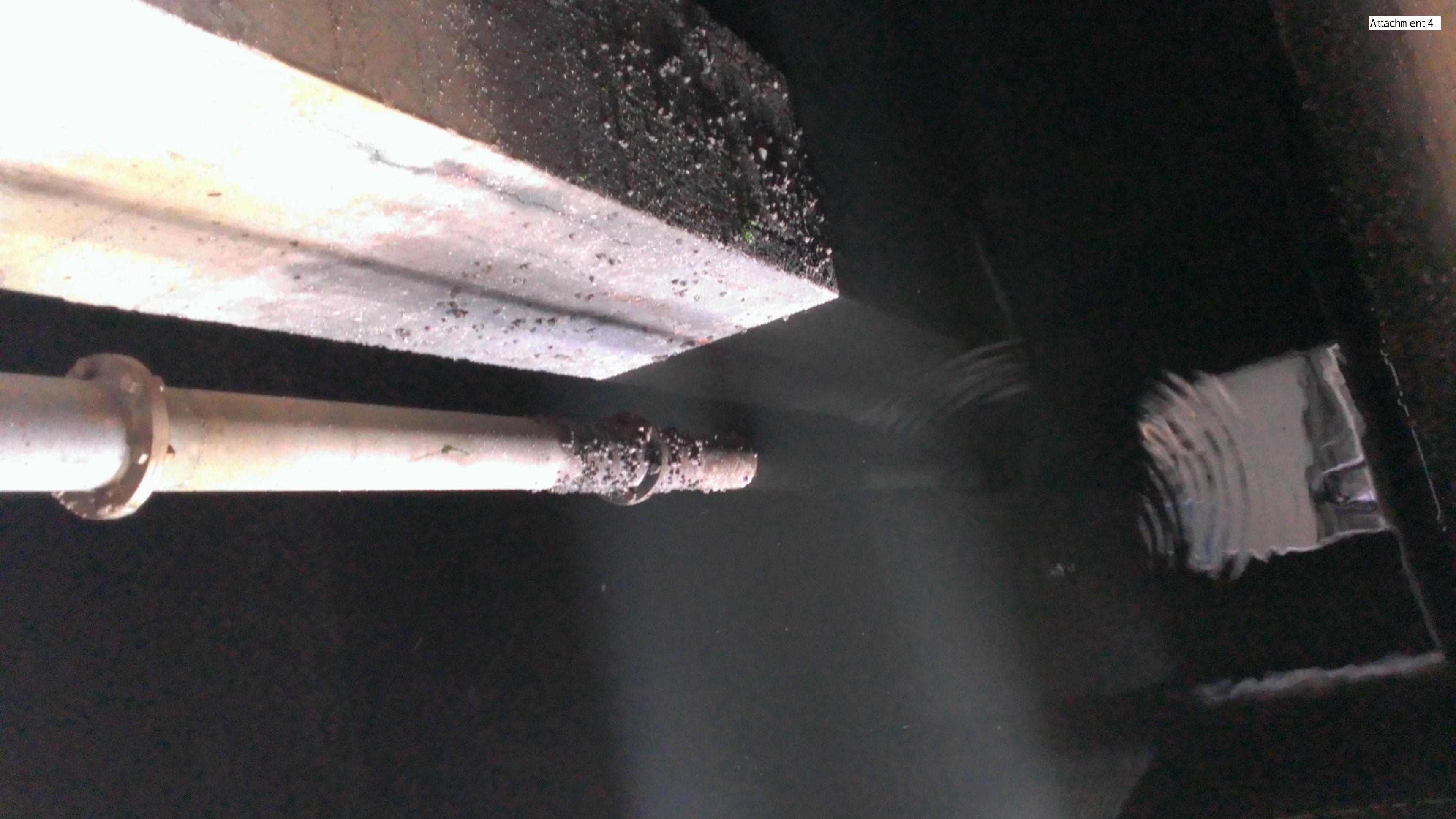
Photo 1 – North Meter Chamber and access point for temporary and permanent meters

ADS NEMA

4x

Photo 4 – East Meter Chamber and access point for temporary meters

ADS NEMA

4x

Attachment 2

Analytical Procedures

Coliforms—Fecal

Page 1 of 8

Coliforms—Fecal, MF, m-FC and m-FC/RA 8074

Introduction

The Membrane Filtration (MF) method is a fast way to estimate bacterial populations in water. The

MF method is especially useful when evaluating large sample volumes or performing many

coliform tests daily.

Method

In the initial step, an appropriate sample volume passes through a membrane filter with a pore size

small enough (0.45 micron) to retain the bacteria present. The filter is placed on an agar plate

prepared with a culture medium that is selective for coliform growth. The petri dish is incubated,

upside down, for 24 hours at the appropriate temperature. After incubation, the colonies that have

grown are identified and counted using a low-power microscope.

PourRite™ Ampules contain prepared selective media. This eliminates the measuring, mixing, and

autoclaving needed when preparing dehydrated media. The ampules are designed with a large,

unrestrictive opening that allows media to pour out easily. Each ampule contains enough medium

for one test.

Nonpotable waters procedures

Wastewater, river, bathing, and other nonpotable waters usually are tested for fecal coliforms. In

testing for fecal coliforms, a special medium and an elevated incubation temperature inhibit growth

of nonfecal coliforms. Fecal coliforms growing on the membrane form an acid that reacts with an

aniline dye in the medium, producing a blue color.

Use m-FC Broth with Rosolic Acid to increase specificity when high levels of non-coliform bacteria

may be present, unless all the organisms in the sample are stressed or injured.

Coliforms—Fecal DOC316.53.001209

USEPA Membrane Filtration Method Method 80741

1 USEPA approved 9222 D.

m-FC and m-FC/RA

Scope and Application: For potable water, nonpotable water, recreation water and wastewater.

Test preparation

Before starting the test:

When the sample is less than 20 mL (diluted or undiluted), add 10 mL of sterile dilution water to the filter funnel before

applying the vacuum. This aids in distributing the bacteria evenly across the entire filter surface.

The volume of sample to be filtered will vary with the sample type. Select a maximum sample size to give 20 to 200

colony-forming units (CFU) per filter. The ideal sample volume of nonpotable water or wastewater for coliform testing yields

20–80 coliform colonies per filter. Generally, for finished, potable water, the volume to be filtered will be 100 mL.

If using PourRite™ ampules, allow the media to warm to room temperature before opening.

Disinfect the work bench with a germicidal cloth, dilute bleach solution, bactericidal spray or dilute iodine solution. Wash

hands thoroughly with soap and water.

Coliforms—Fecal

Page 2 of 8

Coliforms—Fecal

Confirmation of fecal coliforms (m-FC or m-FC/RA), method 8074

1. Place a sterile

absorbent pad in a sterile

petri dish using sterilized

forceps. Replace the petri

dish lid.

Do not touch the pad or

the inside of the petri dish.

To sterilize forceps, dip

forceps in alcohol and

flame in an alcohol or

Bunsen burner. Let

forceps cool before use.

Petri dishes with pads are

available.

2. Invert an m-FC Broth

PourRite Ampule 2 to 3

times to mix the broth. Use

the ampule breaker to

open an ampule. Carefully

pour the contents evenly

onto the absorbent pad.

Replace the petri dish lid.

Use m-FC Broth with

Rosolic Acid to increase

specificity when high

levels of non-coliform

bacteria may be present,

unless the organisms are

stressed or injured.

3. Set up the Membrane

Filter Assembly. Use

sterilized forceps to place

a membrane filter, grid

side up, into the assembly.

4. Prepare the necessary

dilutions to obtain the

proper sample size. Invert

the sample for 30 seconds

to mix. Pour sample into

the funnel. Apply vacuum

and filter the sample.

Rinse the funnel walls with

20 to 30 mL of sterile

buffered dilution water.

Apply vacuum. Repeat

rinsing step, two more

times.

Release the vacuum when

the filter is dry to prevent

damage to the filter.

5. Turn off the vacuum

and lift off the funnel top.

Use sterile forceps to

transfer the membrane

filter to the previously

prepared petri dish.

6. With a slight rolling

motion, center the filter,

grid side up, on the

absorbent pad. Check for

air trapped under the filter

and make sure the entire

filter touches the pad.

Replace the petri dish lid.

7. Invert the petri dish

and incubate at

44.5 ± 0.2 °C for

24 ± 2 hours.

To eliminate environmental

Klebsiella from the fecal

coliform population elevate

the temperature to

45.0 ± 0.2 °C.

Alternatively, a water bath

with rack may be used for

incubation by placing the

petri dishes into a sealed

bag.

8. After incubating, count

the blue colonies using a

10 to 15X microscope.

Coliforms—Fecal

Coliforms—Fecal

Page 3 of 8

Confirmation of total coliforms (Lauryl Tryptose and Brilliant Green Bile)

For potable water samples, confirm typical colonies to ensure they are coliforms. (Confirm sheen

colonies, up to a maximum of five.) Inoculate parallel tubes of Lauryl Tryptose (LT) Single Strength

(SS) Broth and Brilliant Green Bile (BGB) Broth by transferring growth from each colony. Growth

and gas production in both tubes verifies that the suspect organisms are coliforms. Most Probable

Number (MPN) coliform tubes are ideal for this purpose.

Use the swabbing technique for fecal coliforms or E. coli:

• When determining only the presence or absence of total coliforms

• When inoculating EC or EC/MUG media

Inoculate in this order:

1. EC or EC/MUG

2. LT SS Broth

3. BGB

9. Record the results of the test. See Interpreting and

reporting results.

To verify results, follow Verifying fecal coliforms, method

8074

Confirmation of fecal coliforms (m-FC or m-FC/RA), method 8074 (continued)

Coliforms—Fecal

Page 4 of 8

Coliforms—Fecal

Confirmation of total coliforms (LT and BGB), method 8074

1. Sterilize an inoculating

needle, or use a sterile,

disposable inoculating

needle.

To sterilize an inoculating

needle, heat to red hot in

an alcohol or Bunsen

burner. Let the needle cool

before use.

2. Touch the needle to

the coliform (sheen)

colony grown on m-Endo

Broth. Transfer to a single-

strength Lauryl Tryptose

(LT) Broth tube.

3. Again touch the same

coliform colony with the

needle. Transfer to a

Brilliant Green Bile (BGB)

Broth tube.

4. Invert both tubes to

eliminate any air bubbles

trapped in the inner vials.

Incubate the tubes at

35 ± 0.5 °C. After one

hour, invert the tubes to

remove trapped air in the

inner vial, then continue

incubation.

5. After 24 ± 2 hours,

check the inner vials for

growth and gas bubbles.

Growth (turbidity) and gas

bubbles in both the LT and

BGB Broth tubes verify

that the colonies are

coliforms. If one or both

tubes do not show gas,

continue incubating both

tubes for an additional

24 hours

6. If no gas is present in

the LT Broth tube after

48 hours, the colony is not

a coliform and additional

testing is unnecessary.

Record the results of the

test. See Interpreting and

reporting results

Confirm positive results. If

growth and gas are

produced in the LT Broth

tube but not in the BGB

Broth tube, inoculate

another BGB tube from the

gas-positive LT Broth tube.

Incubate this BGB Broth

tube and check for growth

and gas after 24 hours

and/or after 48 hours. If

growth and gas are

produced within

48 ± 3 hours, the colony is

confirmed as coliform.

Coliforms—Fecal

Coliforms—Fecal

Page 5 of 8

Verifying fecal coliforms, method 8074

1. Sterilize an inoculating

needle, or use a sterile,

disposable inoculating

needle.

To sterilize an inoculating

needle, heat to red hot in

an alcohol or Bunsen

burner flame. Let the

needle cool before use.

2. Touch the needle to a

typical blue colony and

transfer to a Lauryl

Tryptose (LT) Broth tube.

Repeat steps 1 and 3 for

each test being verified.

Steps 3 and 4 can be

performed simultaneously

if multiple incubators are

available.

3. Invert the tubes to

eliminate air trapped

inside the inner vials.

Incubate the tubes at

35 ± 0.5 °C. After one



inner vial and continue

incubation. Check tubes

for growth and gas

production at 24 hours.

If no change has occurred,

continue incubation for

another 24 hours.

If growth and gas are not

produced in 48 ± 3 hours,

the colony was not

coliform. If growth and gas

are produced in

48 ± 3 hours, use a sterile

loop to inoculate one

EC Medium Broth tube

from each gas-positive LT

Broth tube.

4. Invert the tubes to

eliminate air trapped

inside the inner vials.

Incubate the EC Medium

tubes at 44.5 ± 0.2 °C for

24 ±2 hours. After one



inner vial.

5. Growth and gas production at 44.5 °C within

24 ± 2 hours confirms the presence of fecal coliforms.

Record the results of the test. See Interpreting and

reporting results.

Coliforms—Fecal

Page 6 of 8

Coliforms—Fecal

Interpreting and reporting results

Report coliform density as the number of colonies per 100 mL of sample. For total coliforms, use

samples that produce 20 to 80 coliform colonies, and not more than 200 colonies of all types, per

membrane to compute coliform density. For fecal coliform testing, samples should produce 20 to

60 fecal coliform colonies.

Use Equation A to calculate coliform density. Note that “mL sample” refers to actual sample

volume, and not volume of the dilution.

Equation A—Coliform density on a single membrane filter

• If growth covers the entire filtration area of the membrane, or a portion of it, and colonies are

not discrete, report results as “Confluent Growth With or Without Coliforms.”

• If the total number of colonies (coliforms plus non-coliforms) exceeds 200 per membrane or

the colonies are too indistinct for accurate counting, report the results as “Too Numerous To

Count” (TNTC).

In either case, run a new sample using a dilution that will give about 50 coliform colonies and not

more than 200 colonies of all types.

When testing nonpotable water, if no filter meets the desired minimum colony count, calculate the

average coliform density with Equation B.

Equation B—Average coliform density for 1) duplicates, 2) multiple dilutions, or 3) more

than one filter/sample

Controls:

Positive and negative controls are important. Pseudomonas aeruginosa is recommended as a

negative control and Escherichia coli as a positive control. Use the AQUA QC-STIK™ Device for

quality control procedures. Instructions for use come with each AQUA QC-STIK Device.

Potable water samples from municipal treatment facilities should be negative for total coliforms

and fecal coliforms.

Consumables and replacement items

Confirmation of fecal coliforms (m-FC or m-FC/RA)

Required media and reagents

Description Unit Catalog number

m-FC prepared agar plates 15/pkg 2811515

m-FC Broth Ampules, plastic 50/pkg 2373250

m-FC w/Rosolic Acid Broth Ampules, plastic 50/pkg 2428550

m-FC Broth PourRite™ Ampules (for fecal coliform presumptive) 20/pkg 2373220

m-FC with Rosolic Acid Broth PourRite™ Ampules (fecal coliform presumptive) 20/pkg 2428520

Coliform colonies per 100 mLColiform colonies counted

mL of sample filtered--------------------------------------------------------------------- 100×=

Coliform colonies per 100 mL Sum of colonies in all samples

Sum of volumes (in mL) of all samples----------------------------------------------------------------------------------------------------- 100×=

http://www.hach.com/hc/search.product.details.invoker/PackagingCode=2811515






Coliforms—Fecal

Coliforms—Fecal

Page 7 of 8

Confirmation of total coliforms (brilliant green bile broth and lauryl tryptose broth)

Required apparatus


Ampule Breaker, PourRite™ each 2484600

Counter, hand tally 1 1469600

Dish, Petri, with pad, 47-mm, sterile, disposable, Gelman 100/pkg 1471799

Dish, Petri, with pad, 47-mm, sterile, disposable, Millipore 150/pkg 2936300

Filter Holder, magnetic coupling (use with 24861-00) 1 1352900

Filter Funnel Manifold, aluminum, 3-place (use with 13529-00) 1 2486100

Filters, Membrane, 47-mm, 0.45-µm, gridded, sterile, Gelman 200/pkg 1353001

Filters, Membrane, 47-mm, 0.45-µm, gridded, sterile, Millipore 150/pkg 2936100

Filtering Flask, 1000-mL 1 54653

Forceps, stainless steel 1 2141100

Incubator, Culture, low profile, 110 VAC, 50/60 Hz each 2619200


Inoculating Needle, disposable 25/pkg 2748925

Loop, inoculating, disposable 25/pkg 2749125

Microscope, compound each 2942500

Optional media and reagents


Bags, Whirl-Pak®, without dechlorinating agent, 207 mL 100/pkg 2233199

Incubator, Water Bath, 110 VAC, 50/60 Hz each 2616300

Incubator, Water Bath, 220 VAC, 50/60 Hz each 2616302

Required media and reagents


Brilliant Green Bile Broth Tubes (for total coliform confirmation) 15/pkg 32215

Lauryl Tryptose Broth Ampules, sterile (for enrichment technique) 20/pkg 1472520

Lauryl Tryptose Broth Tubes, single-strength (for total coliform confirmation) 15/pkg 2162315

Required apparatus


Alcohol Burner 1 2087742

Ampule Breaker, PourRite™ each 2484600

Burner, Bunsen each 2162700



Isopropyl alcohol 500 mL 1445949

Loop, inoculating, disposable 25/pkg 2749125

Pad, absorbent, with dispenser 1000/pkg 1491800

HACH COMPANYWORLD HEADQUARTERSTelephone: (970) 669-3050FAX: (970) 669-2932

FOR TECHNICAL ASSISTANCE, PRICE INFORMATION AND ORDERING:Call 800-227-4224

Contact the HACH office or distributor serving you.www.hach.com [email protected]

In the U.S.A. –Outside the U.S.A. –On the Worldwide Web – ; E-mail –

toll-free

Coliforms—Fecal

© Hach Company, 2007, 2010, 2012. All rights reserved. Printed in the U.S.A. Edition 7

Optional media, reagents and apparatus


Adapter for rechargeable battery pack, 230 VAC (for 2580300) each 2595902

Alcohol Burner 1 2087742

Autoclave, 120 VAC, 50/60 Hz each 2898600

Bag, for contaminated items 200/pkg 2463300



Bags, Whirl-Pak®, with dechlorinating agent, 180 mL 100/pkg 2075333

Battery eliminator each 2580400

Battery pack, rechargeable, for portable incubator 12 VDC each 2580300

Bottle, sample, sterilized, 100-mL, disposable with dechlorinating agent 12/pkg 2599112

Bottle, sample, sterilized, 100-mL, disposable with dechlorinating agent 50/pkg 2599150

Bottle, sample, sterilized, 100-mL, disposable 12/pkg 2495012

Bottle, sample, sterilized, 100-mL, disposable 50/pkg 2495050

Dechlorinating Reagent Powder Pillows 100/pkg 1436369

Dish, Petri, 47-mm, sterile, disposable 100/pkg 1485299

Dish, Petri, 47-mm, sterile, disposable 500/pkg 1485200

Filter Funnel Manifold, aluminum, 3-place (use with 13529-00) each 2486100

Filter Unit, sterile, disposable with gridded membrane (use with 2656700) 12/pkg 2656600

Filtration Support (for field use), stainless steel each 2586200

Funnels, Push-Fit and membrane filters (use with 2586200) 72/pkg 2586300

Germicidal Cloths 50/pkg 2463200

Incubator, portable, 12 VDC each 2569900

Pump, vacuum/pressure, portable, 115 VAC, 60 Hz each 2824800

Pump, vacuum/pressure, portable, 220 VAC, 50 Hz each 2824802

Stopper, rubber, one hole, No. 8 6/pkg 211908

Tubing, rubber, 0.8 cm ID 3.7 m (12 ft) 56019

Sterilization Indicator, Sterikon® 15/pkg 2811115

Sterilization Indicator, Sterikon® 100/pkg 2811199

Syringe, 140-mL, polypropylene (use with 2586200) each 2586100

Wicks, replacement, for alcohol burner 2087742 10/pkg 2097810

Method 1600: Enterococci in Water byMembrane Filtration Using membrane-Enterococcus Indoxyl-$-D-Glucoside Agar(mEI)

December 2009

U.S. Environmental Protection AgencyOffice of Water (4303T)

1200 Pennsylvania Avenue, NWWashington, DC 20460

EPA-821-R-09-016

Acknowledgments

This method was developed under the direction of James W. Messer and Alfred P. Dufour of the U.S.Environmental Protection Agency's (EPA) Human Exposure Research Division, National ExposureResearch Laboratory, Cincinnati, Ohio.

The following laboratories are gratefully acknowledged for their participation in the validation of thismethod in wastewater effluents:

Volunteer Research Laboratories• EPA Office of Research and Development, National Risk Management Research Lab: Mark C.

Meckes

• U.S. Army Corps of Engineers, Washington Aqueduct: Elizabeth A. Turner, Michael L.Chicoine, and Lisa Neal

Volunteer Verification Laboratories• City of Los Angeles Bureau of Sanitation: Farhana Mohamed, Ann Dalkey, Ioannice Lee,

Genevieve Espineda, and Zora Bahariance

• Orange County Sanitation District, Environmental Sciences Laboratory: Charles McGee, Michaelvon Winckelmann, Kim Patton, Linda Kirchner, James Campbell, Arturo Diaz, and Lisa McMath

Volunteer Participant Laboratories• City of Los Angeles Bureau of Sanitation: Farhana Mohamed, Ann Dalkey, Ioannice Lee,

Genevieve Espineda, and Zora Bahariance

• County Sanitation Districts of Los Angeles County (JWPCP): Kathy Walker, Michele Padilla,and Albert Soof

• County Sanitation Districts of Los Angeles County (SJC): Shawn Thompson and JulieMillenbach

• Environmental Associates (EA): Susan Boutros and John Chandler

• Hampton Roads Sanitation District (HRSD): Anna Rule, Paula Hogg, and Bob Maunz

• Hoosier Microbiological Laboratories (HML): Don Hendrickson, Katy Bilger, and LindseyShelton

• Massachusetts Water Resources Authority (MWRA): Steve Rhode and Mariya Gofhsteyn

• North Shore Sanitation District (NSSD): Robert Flood

• Texas A&M University: Suresh Pillai and Reema Singh

• University of Iowa Hygienic Laboratory: Nancy Hall and Cathy Lord

• Wisconsin State Laboratory of Hygiene (WSLH): Jon Standridge, Sharon Kluender, LindaPeterson, and Jeremy Olstadt

• Utah Department of Health: Sanwat Chaudhuri and Devon Cole

iii

Disclaimer

Neither the United States Government nor any of its employees, contractors, or their employees make anywarranty, expressed or implied, or assumes any legal liability or responsibility for any third party’s use ofor the results of such use of any information, apparatus, product, or process discussed in this report, orrepresents that its use by such party would not infringe on privately owned rights. Mention of tradenames or commercial products does not constitute endorsement or recommendation for use.

Questions concerning this method or its application should be addressed to:

Robin K. OshiroEngineering and Analysis Division (4303T)U.S. EPA Office of Water, Office of Science and Technology1200 Pennsylvania Avenue, NWWashington, DC [email protected] or [email protected]

iv

Table of Contents

1.0 Scope and Application . . . . . . . . . . . . . . . . . . . . . . . . . . . . . . . . . . . . . . . . . . . . . . . . . . . . . . . . . 1

2.0 Summary of Method . . . . . . . . . . . . . . . . . . . . . . . . . . . . . . . . . . . . . . . . . . . . . . . . . . . . . . . . . . . 1

3.0 Definitions . . . . . . . . . . . . . . . . . . . . . . . . . . . . . . . . . . . . . . . . . . . . . . . . . . . . . . . . . . . . . . . . . . . 2

4.0 Interferences . . . . . . . . . . . . . . . . . . . . . . . . . . . . . . . . . . . . . . . . . . . . . . . . . . . . . . . . . . . . . . . . . 2

5.0 Safety . . . . . . . . . . . . . . . . . . . . . . . . . . . . . . . . . . . . . . . . . . . . . . . . . . . . . . . . . . . . . . . . . . . . . . 2

6.0 Equipment and Supplies . . . . . . . . . . . . . . . . . . . . . . . . . . . . . . . . . . . . . . . . . . . . . . . . . . . . . . . . 2

7.0 Reagents and Standards . . . . . . . . . . . . . . . . . . . . . . . . . . . . . . . . . . . . . . . . . . . . . . . . . . . . . . . . 3

8.0 Sample Collection, Handling, and Storage . . . . . . . . . . . . . . . . . . . . . . . . . . . . . . . . . . . . . . . . . . 7

10.0 Calibration and Standardization . . . . . . . . . . . . . . . . . . . . . . . . . . . . . . . . . . . . . . . . . . . . . . . . . 12

11.0 Procedure . . . . . . . . . . . . . . . . . . . . . . . . . . . . . . . . . . . . . . . . . . . . . . . . . . . . . . . . . . . . . . . . . . 12

13.0 Data Analysis and Calculations . . . . . . . . . . . . . . . . . . . . . . . . . . . . . . . . . . . . . . . . . . . . . . . . . 14

15.0 Method Performance . . . . . . . . . . . . . . . . . . . . . . . . . . . . . . . . . . . . . . . . . . . . . . . . . . . . . . . . . . 19

16.0 Pollution Prevention . . . . . . . . . . . . . . . . . . . . . . . . . . . . . . . . . . . . . . . . . . . . . . . . . . . . . . . . . . 23

17.0 Waste Management . . . . . . . . . . . . . . . . . . . . . . . . . . . . . . . . . . . . . . . . . . . . . . . . . . . . . . . . . . . 23

18.0 References . . . . . . . . . . . . . . . . . . . . . . . . . . . . . . . . . . . . . . . . . . . . . . . . . . . . . . . . . . . . . . . . . . 23

v

List of Appendices

Appendices A and B are taken from Microbiological Methods for Monitoring the Environment, Waterand Wastes (Reference 18.7).

Appendix A: Part II (General Operations), Section A (Sample Collection, Preservation, and Storage).

Appendix B: Part II (General Operations), Sections C.3.5 (Counting Colonies) and C.3.6 (Calculation of Results).

December 20091

Method 1600: Enterococci in Water by Membrane Filtration Usingmembrane-Enterococcus Indoxyl-$-D-Glucoside Agar (mEI)

December 2009

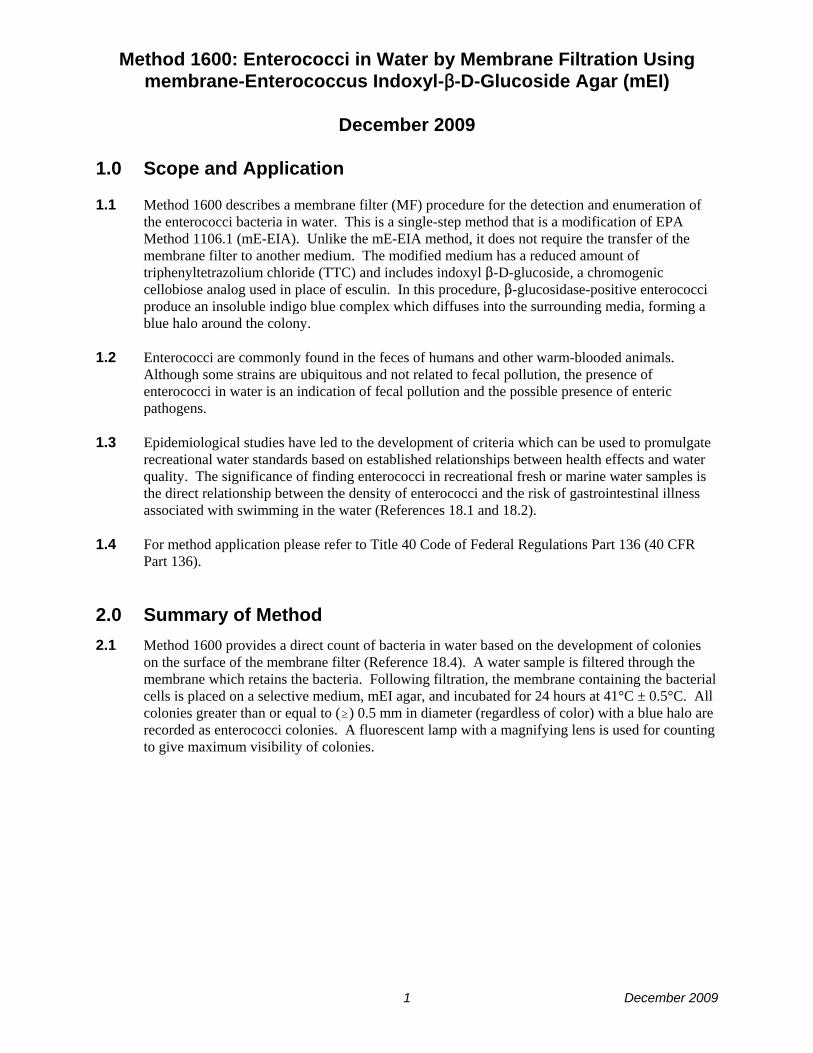
1.0 Scope and Application

1.1 Method 1600 describes a membrane filter (MF) procedure for the detection and enumeration ofthe enterococci bacteria in water. This is a single-step method that is a modification of EPAMethod 1106.1 (mE-EIA). Unlike the mE-EIA method, it does not require the transfer of themembrane filter to another medium. The modified medium has a reduced amount oftriphenyltetrazolium chloride (TTC) and includes indoxyl $-D-glucoside, a chromogeniccellobiose analog used in place of esculin. In this procedure, $-glucosidase-positive enterococciproduce an insoluble indigo blue complex which diffuses into the surrounding media, forming ablue halo around the colony.

1.2 Enterococci are commonly found in the feces of humans and other warm-blooded animals. Although some strains are ubiquitous and not related to fecal pollution, the presence ofenterococci in water is an indication of fecal pollution and the possible presence of entericpathogens.

1.3 Epidemiological studies have led to the development of criteria which can be used to promulgaterecreational water standards based on established relationships between health effects and waterquality. The significance of finding enterococci in recreational fresh or marine water samples isthe direct relationship between the density of enterococci and the risk of gastrointestinal illnessassociated with swimming in the water (References 18.1 and 18.2).

1.4 For method application please refer to Title 40 Code of Federal Regulations Part 136 (40 CFRPart 136).

2.0 Summary of Method2.1 Method 1600 provides a direct count of bacteria in water based on the development of colonies

on the surface of the membrane filter (Reference 18.4). A water sample is filtered through themembrane which retains the bacteria. Following filtration, the membrane containing the bacterialcells is placed on a selective medium, mEI agar, and incubated for 24 hours at 41°C ± 0.5°C. Allcolonies greater than or equal to ($) 0.5 mm in diameter (regardless of color) with a blue halo arerecorded as enterococci colonies. A fluorescent lamp with a magnifying lens is used for countingto give maximum visibility of colonies.

Method 1600

December 2009 2

3.0 Definitions

3.1 In Method 1600, enterococci are those bacteria which produce colonies greater than or equal to0.5 mm in diameter with a blue halo after incubation on mEI agar. The blue halo should not beincluded in the colony diameter measurement. Enterococci include Enterococcus faecalis (E.faecalis), E. faecium, E. avium, E. gallinarium, and their variants. The genus Enterococcusincludes the enterococci formerly assigned to the Group D fecal streptococci.

4.0 Interferences

4.1 Water samples containing colloidal or suspended particulate materials can clog the membranefilter and prevent filtration, or cause spreading of bacterial colonies which could interfere withenumeration and identification of target colonies.

5.0 Safety

5.1 The analyst/technician must know and observe the normal safety procedures required in amicrobiology laboratory while preparing, using, and disposing of cultures, reagents, andmaterials, and while operating sterilization equipment.

5.2 The selective medium (mEI) and azide-dextrose broth used in this method contain sodium azideas well as other potentially toxic components. Caution must be exercised during the preparation,use, and disposal of these media to prevent inhalation or contact with the medium or reagents.

5.3 This method does not address all of the safety issues associated with its use. It is theresponsibility of the laboratory to establish appropriate safety and health practices prior to use ofthis method. A reference file of material safety data sheets (MSDSs) should be available to allpersonnel involved in Method 1600 analyses.

5.4 Mouth-pipetting is prohibited.

6.0 Equipment and Supplies6.1 Glass lens with magnification of 2-5X or stereoscopic microscope

6.2 Lamp, with a cool, white fluorescent tube

6.3 Hand tally or electronic counting device

6.4 Pipet container, stainless steel, aluminum or borosilicate glass, for glass pipets

6.5 Pipets, sterile, T.D. bacteriological or Mohr, glass or plastic, of appropriate volume

6.6 Sterile graduated cylinders, 100-1000 mL, covered with aluminum foil or kraft paper

6.7 Sterile membrane filtration units (filter base and funnel), glass, plastic or stainless steel, wrappedwith aluminum foil or kraft paper

6.8 Ultraviolet unit for sanitization of the filter funnel between filtrations (optional)

Method 1600

December 20093

6.9 Line vacuum, electric vacuum pump, or aspirator for use as a vacuum source (In an emergency orin the field, a hand pump or a syringe equipped with a check valve to prevent the return flow ofair, can be used)

6.10 Flask, filter, vacuum, usually 1 L, with appropriate tubing

6.11 A filter manifold to hold a number of filter bases (optional)

6.12 Flask for safety trap placed between the filter flask and the vacuum source

6.13 Forceps, straight or curved, with smooth tips to handle filters without damage

6.14 Ethanol, methanol or isopropanol in a small, wide-mouth container, for flame-sterilizing forceps

6.15 Burner, Bunsen or Fisher type, or electric incinerator unit for sterilizing loops and needles

6.16 Thermometer, checked against a National Institute of Standards and Technology (NIST) certifiedthermometer, or one that meets the requirements of NIST Monograph SP 250-23

6.17 Petri dishes, sterile, plastic, 9 x 50 mm, with tight-fitting lids; or 15 x 60 mm with loose fittinglids; or 15 x 100 mm with loose fitting lids

6.18 Bottles, milk dilution, borosilicate glass, screw-cap with neoprene liners, 125 mL volume

6.19 Flasks, borosilicate glass, screw-cap, 250-2000 mL volume

6.20 Membrane filters, sterile, white, grid marked, 47 mm diameter, with 0.45 µm pore size

6.21 Platinum wire inoculation loops, at least 3 mm diameter in suitable holders; or sterile plasticloops

6.22 Incubator maintained at 41°C ± 0.5°C

6.23 Waterbath maintained at 50°C for tempering agar

6.24 Test tubes, 20 x 150 mm, borosilicate glass or plastic

6.25 Caps, aluminum or autoclavable plastic, for 20 mm diameter test tubes

6.26 Test tubes, screw-cap, borosilicate glass, 16 x 125 mm or other appropriate size

6.27 Autoclave or steam sterilizer capable of achieving 121°C [15 lb pressure per square inch (PSI)]for 15 minutes

7.0 Reagents and Standards7.1 Purity of Reagents: Reagent grade chemicals shall be used in all tests. Unless otherwise

indicated, reagents shall conform to the specifications of the Committee on Analytical Reagentsof the American Chemical Society (Reference 18.5). The agar used in preparation of culturemedia must be of microbiological grade.

7.2 Whenever possible, use commercial culture media as a means of quality control.

7.3 Purity of reagent water: Reagent-grade water conforming to specifications in: Standard Methodsfor the Examination of Water and Wastewater (latest edition approved by EPA in 40 CFR Part136 or 141, as applicable), Section 9020 (Reference 18.6).

Method 1600

December 2009 4

7.4 Phosphate buffered saline (PBS)

7.4.1 Composition:

Sodium dihydrogen phosphate (NaH2PO4) 0.58 gDisodium hydrogen phosphate (Na2HPO4) 2.5 gSodium chloride (NaCl) 8.5 gReagent-grade water 1.0 L

7.4.2 Dissolve the reagents in 1 L of reagent-grade water and dispense in appropriate amountsfor dilutions in screw cap bottles or culture tubes, and/or into containers for use as rinsewater. Autoclave after preparation at 121°C (15 PSI) for 15 min. Final pH should be 7.4± 0.2.

7.5 mEI Agar

7.5.1 Composition:

Peptone 10.0 gSodium chloride (NaCl) 15.0 gYeast extract 30.0 gEsculin 1.0 gActidione (Cycloheximide) 0.05 gSodium azide 0.15 gIndoxyl $-D-glucoside 0.75 gAgar 15.0 gReagent-grade water 1.0 L

7.5.2 Add reagents to 1 L of reagent-grade water, mix thoroughly, and heat to dissolvecompletely. Autoclave at 121°C (15 PSI) for 15 minutes and cool in a 50°C water bath.

7.5.3 After sterilization add 0.24 g nalidixic acid (sodium salt) and 0.02 g triphenyltetrazoliumchloride (TTC) to the mEI medium and mix thoroughly.

Note: The amount of TTC used in this medium (mEI) is less than the amount used for mEagar in Method 1106.1.

7.5.4 Dispense mEI agar into 9 × 50 mm or 15 × 60 mm petri dishes to a 4-5 mm depth(approximately 4-6 mL), and allow to solidify. Final pH of medium should be 7.1 ± 0.2. Store in a refrigerator.

7.6 Tryptic soy agar (TSA)

7.6.1 Composition:

Pancreatic digest of casein 15.0 gEnzymatic digest of soybean meal 5.0 gSodium chloride (NaCl) 5.0 gAgar 15.0 gReagent-grade water 1.0 L

7.6.2 Add reagents to 1 L of reagent-grade water, mix thoroughly, and heat to dissolvecompletely. Autoclave at 121°C (15 PSI) for 15 minutes and cool in a 50°C waterbath. Pour the medium into each 15 × 60 mm culture dish to a 4-5 mm depth (approximately4-6 mL), and allow to solidify. Final pH should be 7.3 ± 0.2.

Method 1600

December 20095

7.7 Brain heart infusion broth (BHIB)

7.7.1 Composition:

Calf brains, infusion from 200.0 g 7.7 gBeef heart, infusion from 250.0 g 9.8 gProteose peptone 10.0 gSodium chloride (NaCl) 5.0 gDisodium hydrogen phosphate (Na2HPO4) 2.5 gDextrose 2.0 gReagent-grade water 1.0 L

7.7.2 Add reagents to 1 L of reagent-grade water, mix thoroughly, and heat to dissolvecompletely. Dispense in 10-mL volumes in screw cap tubes, and autoclave at 121°C (15PSI) for 15 minutes. Final pH should be 7.4 ± 0.2.

7.8 Brain heart infusion broth (BHIB) with 6.5% NaC1

7.8.1 Composition:

BHIB with 6.5% NaC1 is the same as BHIB above (Section 7.7), but with additionalNaC1.

7.8.2 Add NaCl to formula provided in Section 7.7 above, such that the final concentration is6.5% (65 g NaCl/L). Typically, for commercial BHIB media, an additional 60.0 g NaClper liter of medium will need to be added to the medium. Prepare as in Section 7.7.2.

7.9 Brain heart infusion agar (BHIA)

7.9.1 Composition:

BHIA contains the same components as BHIB (Section 7.7) ,with the addition of 15.0 gagar per liter of BHIB.

7.9.2 Add agar to formula for BHIB provided in Section 7.7 above. Prepare as in Section7.7.2. After sterilization, slant until solid. Final pH should be 7.4 ± 0.2.

Method 1600

December 2009 6

7.10 Bile esculin agar (BEA)

7.10.1 Composition:

Beef Extract 3.0 gPancreatic Digest of Gelatin 5.0 gOxgall 20.0 gEsculin 1.0 gFerric Citrate 0.5 gBacto Agar 14.0 gReagent-grade water 1.0 L

7.10.2 Add reagents to 1 L reagent-grade water, heat with frequent mixing, and boil 1 minute todissolve completely. Dispense 10-mL volumes in tubes for slants or larger volumes intoflasks for subsequent plating. Autoclave at 121°C (15 PSI) for 15 minutes. Overheatingmay cause darkening of the medium. Cool in a 50°C waterbath, and dispense into sterilepetri dishes. Final pH should be 6.8 ± 0.2. Store in a refrigerator.

7.11 Azide dextrose broth (ADB)

7.11.1 Composition:

Beef extract 4.5 gPancreatic digest of casein 7.5 gProteose peptone No. 3 7.5 gDextrose 7.5 gSodium chloride (NaCl) 7.5 gSodium azide 0.2 gReagent-grade water 1.0 L

7.11.2 Add reagents to 1 L of reagent-grade water and dispense in screw cap bottles. Autoclaveat 121°C (15 PSI) for 15 minutes. Final pH should be 7.2 ± 0.2.

7.12 Control cultures

7.12.1 Positive control and/or spiking organism (either of the following are acceptable)

• Stock cultures of Enterococcus faecalis (E. faecalis) ATCC #19433

• E. faecalis ATCC #19433 BioBalls (bioMérieux Inc., Durham NC)

7.12.2 Negative control organism (either of the following are acceptable)

• Stock cultures of Escherichia coli (E. coli) ATCC #11775

• E. coli ATCC #11775 BioBalls (bioMérieux Inc., Durham NC)

Method 1600

December 20097

8.0 Sample Collection, Handling, and Storage

8.1 Sampling procedures are briefly described below. Detailed sampling methods can be found inReference 18.7 (see Appendix A). Adherence to sample preservation procedures and holdingtime limits is critical to the production of valid data. Samples not collected according to theserules should not be analyzed.

8.1.1 Sampling techniques

Samples are collected by hand or with a sampling device if the sampling site has difficultaccess such as a dock, bridge, or bank adjacent to a surface water. Composite samplesshould not be collected, since such samples do not display the range of values found inindividual samples. The sampling depth for surface water samples should be 6-12 inchesbelow the water surface. Sample containers should be positioned such that the mouth ofthe container is pointed away from the sampler or sample point. After removal of thecontainer from the water, a small portion of the sample should be discarded to allow forproper mixing before analyses.

8.1.2 Storage temperature and handling conditions

Ice or refrigerate water samples at a temperature of <10°C during transit to thelaboratory. Do not freeze the samples. Use insulated containers to assure propermaintenance of storage temperature. Take care that sample bottles are not totallyimmersed in water during transit or storage.

8.1.3 Holding time limitations

Sample analysis should begin immediately, preferably within 2 hours of collection. Themaximum transport time to the laboratory is 6 hours, and samples should be processedwithin 2 hours of receipt at the laboratory.

9.0 Quality Control

9.1 Each laboratory that uses Method 1600 is required to operate a formal quality assurance (QA)program that addresses and documents instrument and equipment maintenance and performance,reagent quality and performance, analyst training and certification, and records storage andretrieval. Additional recommendations for QA and quality control (QC) procedures formicrobiological laboratories are provided in Reference 18.7.

9.2 The minimum analytical QC requirements for the analysis of samples using Method 1600 includean initial demonstration of laboratory capability through performance of the initial precision andrecovery (IPR) analyses (Section 9.3), ongoing demonstration of laboratory capability throughperformance of the ongoing precision and recovery (OPR) analysis (Section 9.4) and matrix spike(MS) analysis (Section 9.5, disinfected wastewater only), and the routine analysis of positive andnegative controls (Section 9.6), filter sterility checks (Section 9.8), method blanks (Section 9.9),and media sterility checks (Section 9.11). For the IPR, OPR and MS analyses, it is necessary tospike samples with either laboratory-prepared spiking suspensions or BioBalls as described inSection 14.

Method 1600

December 2009 8

Note: Performance criteria for Method 1600 are based on the results of the interlaboratoryvalidation of Method 1600 in PBS and disinfected wastewater matrices. The IPR (Section 9.3)and OPR (Section 9.4) recovery criteria (Table 1) are valid method performance criteria thatshould be met, regardless of the matrix being evaluated, the matrix spike recovery criteria(Section 9.5, Table 2) pertain only to disinfected wastewaters.

9.3 Initial precision and recovery (IPR)—The IPR analyses are used to demonstrate acceptablemethod performance (recovery and precision) and should be performed by each laboratory beforethe method is used for monitoring field samples. EPA recommends but does not require that anIPR be performed by each analyst. IPR samples should be accompanied by an acceptable methodblank (Section 9.9) and appropriate media sterility checks (Section 9.11). The IPR analyses areperformed as follows:

9.3.1 Prepare four, 100-mL samples of PBS and spike each sample with E. faecalis ATCC#19433 according to the spiking procedure in Section 14. Spiking withlaboratory-prepared suspensions is described in Section 14.2 and spiking with BioBalls isdescribed in Section 14.3. Filter and process each IPR sample according to theprocedures in Section 11 and calculate the number of enterococci per 100 mL accordingto Section 13.

9.3.2 Calculate the percent recovery (R) for each IPR sample using the appropriate equation inSection 14.2.2 or 14.3.4 for samples spiked with laboratory-prepared spiking suspensionsor BioBalls, respectively.

9.3.3 Using the percent recoveries of the four analyses, calculate the mean percent recoveryand the relative standard deviation (RSD) of the recoveries. The RSD is the standarddeviation divided by the mean, multiplied by 100.

9.3.4 Compare the mean recovery and RSD with the corresponding IPR criteria in Table 1,below. If the mean and RSD for recovery of enterococci meet acceptance criteria, systemperformance is acceptable and analysis of field samples may begin. If the mean recoveryor the RSD fall outside of the required range for recovery, system performance isunacceptable. In this event, identify the problem by evaluating each step of the analyticalprocess, media, reagents, and controls, correct the problem and repeat the IPR analyses.

Table 1. Initial and Ongoing Precision and Recovery (IPR and OPR) Acceptance Criteria

Performance test Lab-prepared spikeacceptance criteria

BioBall™ acceptance criteria

Initial precision and recovery (IPR)

• Mean percent recovery

• Precision (as maximum relative standarddeviation)

31% - 127% 85% - 106%

28% 14%

Ongoing precision and recovery (OPR) as percentrecovery

27% - 131% 78% - 113%

Method 1600

December 20099

9.4 Ongoing precision and recovery (OPR)—To demonstrate ongoing control of the analyticalsystem, the laboratory should routinely process and analyze spiked PBS samples. The laboratoryshould analyze one OPR sample after every 20 field and matrix spike samples or one per weekthat samples are analyzed, whichever occurs more frequently. OPR samples must beaccompanied by an acceptable method blank (Section 9.9) and appropriate media sterility checks(Section 9.11). The OPR analysis is performed as follows:

9.4.1 Spike a 100-mL PBS sample with E. faecalis ATCC #19433 according to the spikingprocedure in Section 14. Spiking with laboratory-prepared suspensions is described inSection 14.2 and spiking with BioBalls is described in Section 14.3. Filter and processeach OPR sample according to the procedures in Section 11 and calculate the number ofenterococci per 100 mL according to Section 13.

9.4.2 Calculate the percent recovery (R) for the OPR sample using the appropriate equation inSection 14.2.2 or 14.3.4 for samples spiked with laboratory-prepared spiking suspensionsor BioBalls, respectively.

9.4.3 Compare the OPR result (percent recovery) with the corresponding OPR recoverycriteria in Table 1, above. If the OPR result meets the acceptance criteria for recovery,method performance is acceptable and analysis of field samples may continue. If theOPR result falls outside of the acceptance criteria, system performance is unacceptable. In this event, identify the problem by evaluating each step of the analytical process,media, reagents, and controls, correct the problem and repeat the OPR analysis.

9.4.4 As part of the laboratory QA program, results for OPR and IPR samples should becharted and updated records maintained in order to monitor ongoing methodperformance. The laboratory should also develop a statement of accuracy for Method1600 by calculating the average percent recovery (R) and the standard deviation of thepercent recovery (sr). Express the accuracy as a recovery interval from R - 2sr to R + 2sr.

9.5 Matrix spikes (MS)—MS analysis are performed to determine the effect of a particular matrix

on enterococci recoveries. The laboratory should analyze one MS sample when disinfectedwastewater samples are first received from a source from which the laboratory has not previouslyanalyzed samples. Subsequently, 5% of field samples (1 per 20) from a given disinfectedwastewater source should include a MS sample. MS samples must be accompanied by theanalysis of an unspiked field sample sequentially collected from the same sampling site, anacceptable method blank (Section 9.9), and appropriate media sterility checks (Section 9.11). When possible, MS analyses should also be accompanied by an OPR sample (Section 9.4), usingthe same spiking procedure (laboratory-prepared spiking suspension or BioBalls). The MSanalysis is performed as follows:

9.5.1 Prepare two, 100-mL field samples that were sequentially collected from the same site.One sample will remain unspiked and will be analyzed to determine the background orambient concentration of enterococci for calculating MS recoveries (Section 9.5.3). Theother sample will serve as the MS sample and will be spiked with E. faecalis ATCC#19433 according to the spiking procedure in Section 14.

Method 1600

December 2009 10

9.5.2 Select sample volumes based on previous analytical results or anticipated levelsof in the field sample in order to achieve the recommended target range of enterococci(20-60 CFU, including spike) per filter. If the laboratory is not familiar with the matrixbeing analyzed, it is recommended that a minimum of three dilutions be analyzed toensure that a countable plate is obtained for the MS and associated unspiked sample. Ifpossible, 100-mL of sample should be analyzed.

9.5.3 Spike the MS sample volume(s) with a laboratory-prepared suspension as described inSection 14.2 or with BioBalls as described in Section 14.3. Immediately filter andprocess the unspiked and spiked field samples according to the procedures in Section 11.

Note: When analyzing smaller sample volumes (e.g, <20 mL), 20-30 mL of PBS shouldbe added to the funnel or an aliquot of sample should be dispensed into a 20-30 mLdilution blank prior to filtration. This will allow even distribution of the sample on themembrane.

9.5.4 For the MS sample, calculate the number of enterococci (CFU / 100 mL) according toSection 13 and adjust the colony counts based on any background enterococci observedin the unspiked matrix sample.

9.5.5 Calculate the percent recovery (R) for the MS sample (adjusted based on ambiententerococci in the unspiked sample) using the appropriate equation in Section 14.2.2 or14.3.4 for samples spiked with laboratory-prepared spiking suspensions or BioBalls,respectively.

9.5.6 Compare the MS result (percent recovery) with the appropriate method performancecriteria in Table 2, below. If the MS recovery meets the acceptance criteria, systemperformance is acceptable and analysis of field samples from this disinfected wastewatersource may continue. If the MS recovery is unacceptable and the OPR sample resultassociated with this batch of samples is acceptable, a matrix interference may be causingthe poor results. If the MS recovery is unacceptable, all associated field data should beflagged.

9.5.7 Acceptance criteria for MS recovery (Table 2) are based on data from spiked disinfectedwastewater matrices and are not appropriate for use with other matrices (e.g., ambientwaters).

Table 2. Matrix Spike Precision and Recovery Acceptance Criteria

Performance test Lab-prepared acceptancecriteria

BioBall™ acceptancecriteria

Percent recovery for MS 29% - 122% 63% - 110%

9.5.8 Laboratories should record and maintain a control chart comparing MS recoveries for all matrices to batch-specific and cumulative OPR sample results analyzed using Method

1600. These comparisons should help laboratories recognize matrix effects on methodrecovery and may also help to recognize inconsistent or sporadic matrix effects from aparticular source.

Method 1600

December 200911

9.6 Culture Controls

9.6.1 Negative controls—The laboratory should analyze negative controls to ensure that themEI agar is performing properly. Negative controls should be analyzed whenever a newbatch of media or reagents is used. On an ongoing basis, the laboratory should perform anegative control every day that samples are analyzed.

9.6.1.1 Negative controls are conducted by filtering a dilute suspension of viable E. coli (e.g., ATCC #11775) and analyzing as described in Section 11. Viability of the negative controls should be demonstrated using anon-selective media (e.g., nutrient agar or tryptic soy agar).

9.6.1.2 If the negative control fails to exhibit the appropriate response, check and/orreplace the associated media or reagents, and/or the negative control, andreanalyze the appropriate negative control.

9.6.2 Positive controls—The laboratory should analyze positive controls to ensure that the

mEI agar is performing properly. Positive controls should be analyzed whenever a newbatch of media or reagents is used. On an ongoing basis, the laboratory should perform apositive control every day that samples are analyzed. An OPR sample (Section 9.4) maytake the place of a positive control.

9.6.2.1 Positive controls are conducted by filtering a dilute suspension of viable E. faecalis (e.g., ATCC #19433) and analyzing as described in Section 11.

9.6.2.2 If the positive control fails to exhibit the appropriate response, check and/or replace the associated media or reagents, and/or the positive control, and

reanalyze the appropriate positive control.

9.6.3 Controls for verification media—All verification media should be tested withappropriate positive and negative controls whenever a new batch of media and/orreagents are used. On an ongoing basis, the laboratory should perform positive andnegative controls on the verification media with each batch of samples submitted toverification. Examples of appropriate controls for verification media are provided inTable 3.

Table 3. Verification ControlsMedium Positive Control Negative Control

Bile esculin agar (BEA) E. faecalis E. coli

Brain heart infusion broth (BHIB) with 6.5% NaCl E. faecalis E. coli

Brain heart infusion broth (BHIB) incubated at 45°C E. faecalis E. coli

9.7 Colony verification—The laboratory should verify 10 typical colonies (positive) and 10 atypicalcolonies (negative) per month or 1 typical colony and 1 atypical colony from 10% of all positivesamples, whichever is greater. Verification procedures are provided in Section 12.0.

Method 1600

December 2009 12

9.8 Filter sterility check—Place at least one membrane filter per lot of filters on a TSA plate, andincubate for 24 ± 2 hours at 35°C ± 0.5°C. Absence of growth indicates sterility of the filter. Onan ongoing basis, the laboratory should perform a filter sterility check every day that samples are analyzed.

9.9 Method blank—Filter a 50-mL volume of sterile PBS and place the filter on a mEI agar plateand process according to Section 11.0. Absence of growth indicates freedom of contaminationfrom the target organism. On an ongoing basis, the laboratory should perform a method blankevery day that samples are analyzed.

9.10 Filtration blank—Filter a 50-mL volume of sterile PBS before beginning sample filtrations.Place the filter on a TSA plate, and incubate for 24 ± 2 hours at 35°C ± 0.5°C. Absence ofgrowth indicates sterility of the PBS buffer and filtration assembly.

9.11 Media sterility check—The laboratory should test media sterility by incubating one unit (tubeor plate) from each batch of medium (TSA, mEI agar, and verification media) as appropriate andobserving for growth. Absence of growth indicates media sterility. On an ongoing basis, thelaboratory should perform a media sterility check every day that samples are analyzed.

9.12 Analyst colony counting variability—Laboratories with two or more analysts should compareeach analyst's colony counts from one positive field sample per month. Colony counts should bewithin 10% between analysts. Laboratories with a single analyst should have that analystperform duplicate colony counts of a single membrane filter each month. Duplicate colonycounts should be within 5% for a single analyst. If no positive field samples are available, a OPRsample may be substituted for these determinations.

10.0 Calibration and Standardization

10.1 Check temperatures in incubators twice daily with a minimum of 4 hours between each reading toensure operation within stated limits.

10.2 Check thermometers at least annually against a NIST certified thermometer or one that meets therequirements of NIST Monograph SP 250-23. Check mercury columns for breaks.

10.3 Refrigerators used to store media and reagents should be monitored daily to ensure propertemperature control.

11.0 Procedure

11.1 Prepare the mEI agar as directed in Section 7.6.

11.2 Mark the petri dishes and report forms with sample identification and sample volumes.

11.3 Place a sterile membrane filter on the filter base, grid-side up and attach the funnel to the base sothat the membrane filter is now held between the funnel and the base.

11.4 Shake the sample bottle vigorously about 25 times to distribute the bacteria uniformly, andmeasure the desired volume of sample or dilution into the funnel.

Method 1600

December 200913

11.5 Select sample volumes based on previous knowledge of the enterococci level, to produce 20-60enterococci colonies on membranes. It is recommended that a minimum of three dilutions beanalyzed to ensure that a countable plate (20-60 enterococci colonies) is obtained.

11.6 Smaller sample size or sample dilutions can be used to minimize the interference of turbidity orfor high bacterial densities. Multiple volumes of the same sample or sample dilutions may befiltered.

Note: When analyzing smaller sample volumes (e.g., <20 mL), 20-30 mL of PBS or phosphate-buffered dilution water should be added to the funnel or an aliquot of sample should be dispensedinto a dilution blank prior to filtration. This will allow even distribution of the sample on themembrane.

11.7 Filter the sample, and rinse the sides of the funnel at least twice with 20-30 mL of sterile bufferedrinse water. Turn off the vacuum and remove the funnel from the filter base.

11.8 Use sterile forceps to aseptically remove the membrane filter from the filter base, and roll it ontothe mEI Agar to avoid the formation of bubbles between the membrane and the agar surface.Reseat the membrane if bubbles occur. Run the forceps around the edge of the filter outside thearea of filtration, close to the edge of the dish, to be sure that the filter is properly seated on theagar. Close the dish, invert, and incubate at 41°C ± 0.5°C for 24 ± 2 hours.

Note: If the medium is prepared in 15 × 60 mm loose lid petri dishes, they should be incubated ina tight fitting container (e.g., plastic vegetable crisper) containing a moistened paper towel toprevent dehydration of the membrane filter and medium.

11.9 After incubation, count and record colonies on those membrane filters containing, if practical,20-60 colonies $0.5 mm in diameter with a blue halo regardless of colony color as an enterococci(see Figure 1). Note: When measuring colony size do not include the halo. Use magnification forcounting and a small fluorescent lamp to give maximum visibility of colonies.

Figure 1. Enterococci colonies on mEI produce blue halos.

12.0 Verification Procedure

12.1 Colonies $0.5 mm in diameter of any color having a blue halo after incubation on mEI agar areconsidered to be “typical” enterococci colonies. Verification of colonies may be required inevidence gathering and it is also recommended as a means of quality control. The verificationprocedure follows.

Method 1600

December 2009 14

Note: When evaluating wastewater using Method 1600, it is recommended that the false negativerate for each matrix be evaluated through biochemical confirmation and results adjustedaccordingly, especially if large numbers of atypical colonies are observed in a particular matrix.

12.2 Using a sterile inoculating loop or needle, transfer growth from the centers of at least 10well-isolated typical and at least 10 well-isolated atypical colonies into a BHIB tube and onto aBHIA slant. Incubate broth for 24 ± 2 hours and agar slants for 48 ± 3 hours at 35°C ± 0.5°C.

12.3 After a 24 hour incubation, transfer a loopful of growth from each BHIB tube to BEA, BHIB, andBHIB with 6.5% NaCl.

12.3.1 Incubate BEA and BHIB with 6.5% NaCl at 35°C ± 0.5°C for 48 ± 3 hours.

12.3.2 Incubate BHIB at 45°C ± 0.5°C for 48 ± 3 hours.

12.4 Observe all verification media for growth.

12.5 After 48 hour incubation, perform a Gram stain using growth from each BHIA slant.

12.6 Gram-positive cocci that grow and hydrolyze esculin on BEA (i.e., produce a black or brownprecipitate), and grow in BHIB with 6.5% NaCl at 35°C ± 0.5°C and BHIB at 45°C ± 0.5°C areverified as enterococci.

12.7 Alternately, commercially available multi-test identification systems (e.g., Vitek®) may be usedto verify colonies. Such multi-test identification systems should include esculin hydrolysis andgrowth in 6.5% NaCl.

13.0 Data Analysis and Calculations

Use the following general rules to calculate the enterococci count per 100 mL of sample:

13.1 If possible, select a membrane filter with 20-60 colonies $0.5 mm in diameter (regardless ofcolony color) with a blue halo. Calculate the number of enterococci per 100 mL according to thefollowing general formula:

Enterococci / 100 mL =Number of enterococci colonies

× 100Volume of sample filtered (mL)

13.2 See general counting rules in Reference 18.7 (see Appendix B).

13.3 Report results as enterococci per 100 mL of sample.

Method 1600

December 200915

14.0 Sample Spiking Procedure

14.1 Method 1600 QC requirements (Section 9.0) include the preparation and analysis of spikedreference (PBS) and matrix samples in order to monitor initial and ongoing method performance. For the IPR (Section 9.3), OPR (Section 9.4), and MS (Section 9.5) analyses it is necessary tospike samples with either laboratory-prepared spiking suspensions (Section 14.2) or BioBalls(Section 14.3) as described below.

14.2 Laboratory-Prepared Spiking Suspensions

14.2.1 Preparation

14.2.1.1 Stock Culture. Prepare a stock culture by inoculating a TSA slant (or othernon-selective media) with E. faecalis ATCC #19433 and incubating at 35°C ± 3°C for 20 ± 4 hours. This stock culture may be stored in the dark atroom temperature for up to 30 days.

14.2.1.2 Undiluted Spiking Suspension. Prepare a 1% solution of azide dextrosebroth (ADB) by combining 99 mL of sterile phosphate buffered saline and 1mL of sterile single strength azide dextrose broth in a sterile screw cap bottleor re-sealable dilution water container. From the stock culture of E. faecalisATCC #19433 in Section 14.2.1.1, transfer a small loopful of growth to the 1% azide dextrose broth solution and vigorously shake a minimum of 25times. Disperse the inoculum by vigorously shaking the broth culture andincubate at 35°C ± 3°C for 20 ± 4 hours. This culture is referred to as theundiluted spiking suspension and should contain approximately 1.0 × 106 -1.0 × 107 E. faecalis colony forming units (CFU) per mL of culture.

14.2.1.3 Mix the undiluted spiking suspension (Section 14.2.1.2) thoroughly byshaking the bottle a minimum of 25 times and prepare a series of dilutions (4total) in the following manner:

14.2.1.3.1 Dilution "A"—Aseptically transfer 1.0 mL of the undilutedspiking suspension to 99 mL of sterile PBS and mix thoroughlyby shaking the bottle a minimum of 25 times. This is spikingsuspension dilution "A" and 1 mL contains 10-2 mL of theoriginal undiluted spiking suspension.

14.2.1.3.2 Dilution "B"—Aseptically transfer 1.0 mL of dilution "A" to 99mL of sterile PBS and mix thoroughly by shaking the bottle aminimum of 25 times. This is spiking suspension dilution "B"and 1 mL contains 10-4 mL of the original undiluted spikingsuspension.

14.2.1.3.3 Dilution "C"—Aseptically transfer 11.0 mL of dilution "B" to 99mL of sterile PBS and mix thoroughly by shaking the bottle aminimum of 25 times. This is spiking suspension dilution "C"and 1 mL contains 10-5 mL of the original undiluted spikingsuspension.

14.2.1.3.4 Dilution "D"—Aseptically transfer 11.0 mL of dilution "C"

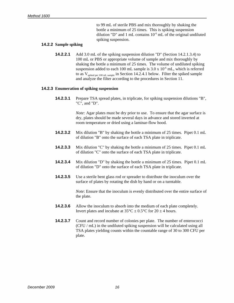
Method 1600

December 2009 16

to 99 mL of sterile PBS and mix thoroughly by shaking thebottle a minimum of 25 times. This is spiking suspensiondilution "D" and 1 mL contains 10-6 mL of the original undilutedspiking suspension.

14.2.2 Sample spiking

14.2.2.1 Add 3.0 mL of the spiking suspension dilution "D" (Section 14.2.1.3.4) to100 mL or PBS or appropriate volume of sample and mix thoroughly byshaking the bottle a minimum of 25 times. The volume of undiluted spikingsuspension added to each 100 mL sample is 3.0 x 10-6 mL, which is referredto as Vspiked per 100 mL sample in Section 14.2.4.1 below. Filter the spiked sampleand analyze the filter according to the procedures in Section 11.

14.2.3 Enumeration of spiking suspension

14.2.3.1 Prepare TSA spread plates, in triplicate, for spiking suspension dilutions "B","C", and "D".

Note: Agar plates must be dry prior to use. To ensure that the agar surface isdry, plates should be made several days in advance and stored inverted atroom temperature or dried using a laminar-flow hood.

14.2.3.2 Mix dilution "B" by shaking the bottle a minimum of 25 times. Pipet 0.1 mLof dilution "B" onto the surface of each TSA plate in triplicate.

14.2.3.3 Mix dilution "C" by shaking the bottle a minimum of 25 times. Pipet 0.1 mLof dilution "C" onto the surface of each TSA plate in triplicate.

14.2.3.4 Mix dilution "D" by shaking the bottle a minimum of 25 times. Pipet 0.1 mLof dilution "D" onto the surface of each TSA plate in triplicate.

14.2.3.5 Use a sterile bent glass rod or spreader to distribute the inoculum over thesurface of plates by rotating the dish by hand or on a turntable.

Note: Ensure that the inoculum is evenly distributed over the entire surface ofthe plate.

14.2.3.6 Allow the inoculum to absorb into the medium of each plate completely. Invert plates and incubate at 35°C ± 0.5°C for 20 ± 4 hours.

14.2.3.7 Count and record number of colonies per plate. The number of enterococci(CFU / mL) in the undiluted spiking suspension will be calculated using allTSA plates yielding counts within the countable range of 30 to 300 CFU perplate.

Method 1600

December 200917

14.2.4 Recovery calculations for spiked samples

14.2.4.1 Calculate the concentration of enterococci (CFU / mL) in the undilutedspiking suspension (Section 14.2.1.2) according to the following equation. Example calculations are provided in Table 4, below.

Enterococci undiluted spike = (CFU1 + CFU2 + ...+ CFUn) / (V1 + V2 + ... + Vn)

Enterococci undiluted spike = Enterococci (CFU / mL) in undiluted spiking suspension

Where,

CFU = Number of colony forming units from TSA plates yielding counts within thecountable range of 30 to 300 CFU per plate

V = Volume of undiluted sample on each TSA plate yielding counts within thecountable range of 30 to 300 CFU per plate

n = Number of plates with counts within the countable range of 30 to 300 CFUper plate

Note: The example calculated numbers provided in the tables below have been roundedat the end of each step for simplification purposes. Generally, rounding should onlyoccur after the final calculation.

Table 4. Example Calculations of Laboratory-prepared Enterococci Spiking Concentration

ExamplesCFU / plate (triplicate analyses) from

TSA plates Enterococci CFU / mL in undiluted spiking suspension

(Enterococci undiluted spike) a10-5 mL plates 10-6 mL plates 10-7 mL plates

Example 1 94, 106, 89 9, 11, 28 1, 0, 4

(94+106+89) / (10-5+10-5+10-5) =

289 / (3.0 x 10-5) = 9,633,333 =

9.6 x 106 CFU / mL

Example 2 32, 55, 72 8, 5, 3 0, 0, 0

(32+55+72) / (10-5+10-5+10-5) =

159 / (3.0 x 10-5) = 5,300,000 =

5.3 x 106 CFU / mL

a Enterococci undiluted spike is calculated using all plates yielding counts within the countable range of 30to 300 CFU per plate

Method 1600

December 2009 18

14.2.4.1 Calculate true concentration of spiked enterococci (CFU / 100 mL)according to the following equation. Example calculations are provided inTable 5, below.

Tspiked Enterococci = (Enterococci undiluted spike) x (V spiked per 100 mL sample)

Where,Tspiked Enterococci = Number of spiked Enterococci (CFU / 100 mL)Enterococci undiluted spike = Enterococci (CFU / mL) in undiluted spiking suspensionV spiked per 100 mL sample = mL of undiluted spiking suspension per 100 mL sample

Table 5. Example Calculations for Determination “True” Spiked Enterococci Concentration

Enterococci undiluted spike V spiked per 100 mL sample Tspiked Enterococci

9.6 x 106 CFU / mL 3.0 X 10-6 mL per 100 mL ofsample

(9.6 x 106 CFU / mL) x (3.0 x 10-6 mL / 100 mL) = 28.8 CFU / 100 mL

5.3 x 106 CFU / mL 3.0 X 10-6 mL per 100 mL ofsample

(2.8 x 106 CFU / mL) x (3.0 x 10-6 mL / 100 mL) = 8.4 CFU / 100 mL

14.2.4.2 Calculate percent recovery (R) of spiked enterococci (CFU / 100 mL)according to the following equation. Example calculations are provided inTable 6, below.

R = 100 x (Ns - Nu)

T

Where,R = Percent recoveryNs = Enterococci (CFU / 100 mL) in the spiked sample (Section 13)Nu = Enterococci (CFU / 100 mL) in the unspiked sample (Section 13)T = True spiked enterococci (CFU / 100 mL) in spiked sample (Section 14.2.4.1)

Table 6. Example Percent Recovery Calculations for Lab-prepared Spiked Samples

Ns (CFU / 100 mL) Nu (CFU / 100 mL) Tspiked Enterococci (CFU / 100 mL) Percent recovery (R)

42 <1 28.8100 x (42 - 1) / 28.8

= 142%

34 10 28.8100 x (34 - 10) / 28.8

= 83%

10 <1 8.4 100 x (10 - 1) / 8.4= 107%

Method 1600

December 200919

14.3 BioBall™ Spiking Procedure

14.3.1 Aseptically add 1 BioBall™ to 100 mL of PBS or appropriate volume of sample and mixby vigorously shaking the sample bottle a minimum of 25 times. Analyze the spikedsample according to the procedures in Section 11.

14.3.2 Recovery calculations for samples spiked with BioBalls—Calculate percent recovery (R)of spiked enterococci (CFU / 100 mL) according to the following equation. Examplecalculations are provided in Table 7, below.

R = 100 x (Ns - Nu)

T

Where,R = Percent recoveryNs = Enterococci (CFU / 100 mL) in the spiked sample (Section 13)Nu = Enterococci (CFU / 100 mL) in the unspiked sample (Section 13)T = True spiked enterococci (CFU / 100 mL) in spiked sample based on the

lot mean value provided by manufacturer

Table 7. Example BioBall™ Percent Recovery Calculations

Ns (CFU / 100 mL) Nu (CFU / 100 mL) T (CFU / 100 mL) Percent recovery (R)

24 <1 32 100 × (24 - 1) / 32 = 72%

36 10 32 100 × (36 - 10) / 32 = 81%

15.0 Method Performance

15.1 Performance Characteristics (Reference 18.4)

15.1.1 Precision - The degree of agreement of repeated measurements of the same parameterexpressed quantitatively as the standard deviation or as the 95% confidence limits of themean computed from the results of a series of controlled determinations. The precisionamong laboratories for marine water and surface water was 2.2% and 18.9%,respectively.

15.1.2 Bias - The persistent positive or negative deviation of the results from the assumed oraccepted true value. The persistent positive or negative deviation of the results from theassumed or accepted true value was not significant.

Method 1600

December 2009 20

15.1.3 Specificity - The ability of a method to select and/or distinguish the target bacteria fromother bacteria in the same water sample. The specificity characteristic of a method isusually reported as the percent of false positive and false negative results. The specificityfor this medium as reported for various environmental water samples was 6.0% falsepositive and 6.5% false negative.

15.1.4 Multilaboratory variability - A collaborative study was conducted among fourteencollaborators at twelve laboratories to examine the interlaboratory reproducibility of themethod. Reproducibility among laboratories (RSDR) for freshwater, marine water,chlorinated secondary effluent, and non-chlorinated primary effluent ranged from 2.2%for marine water to 18.9% for freshwater with a low enterococcal density.

15.2 Interlaboratory Validation of Method 1600 in Disinfected Wastewater (Reference 18.3)

15.2.1 Twelve volunteer participant laboratories, two enterococci verification laboratories, andtwo research laboratories participated in the U.S. Environmental Protection Agency's(EPA's) interlaboratory validation study of EPA Method 1600. The purposes of the studywere to characterize method performance across multiple laboratories and disinfectedwastewater matrices and to develop quantitative quality control (QC) acceptance criteria. A detailed description of the of the study and results are provided in the validation studyreport (Reference 18.3). Results submitted by laboratories were validated using astandardized data review process to confirm that results were generated in accordancewith study-specific instructions and the September 2002 version of EPA Method 1600.

15.2.2 Recovery - Method 1600 was characterized by mean laboratory-specific recoveries ofenterococci from disinfected wastewater samples spiked with BioBalls™ ranging from77.1% to 114.9%, with an overall mean recovery of 90.8%. Mean laboratory-specificrecoveries of enterococci from PBS samples spiked with BioBalls ranged from 88.0% to105.1%, with an overall mean recovery of 95.4%.

15.2.3 Precision - Method 1600 was characterized by laboratory-specific relative standarddeviations (RSDs) from disinfected wastewater samples spiked with BioBalls™ rangingfrom 0% to 69.5%, with an overall pooled, within-laboratory RSD of 22.6%. For PBSsamples spiked with BioBalls, laboratory-specific RSDs ranged from 3.1% to 13.7%,with an overall pooled, within-laboratory RSD of 8.1%.

15.2.4 False positive confirmation rates - Method 1600 laboratory-specific false positiveconfirmation rates for unspiked disinfected/secondary results combined, ranging from0.0% to 10.0%. For secondary wastewater (excluding disinfected results), only 2 of 123typical colonies submitted to verification were non-enterococci, resulting in a falsepositive confirmation rate of 1.6%. For disinfected wastewater (excluding secondaryresults), none of the 66 typical colonies submitted to verification were non-enterococci,resulting in a false positive confirmation rate of 0.0%. Since all 2184 typical coloniesobserved during the study could not be submitted to confirmation, the percent of totalcolonies that would have resulted in a false positive result was estimated (see Table 6,Reference 18.3). It is estimated that 0.0% and 1.2% of the total colonies would haveresulted in a false positive for disinfected wastewater and secondary wastewater,respectively.

Method 1600

December 200921

15.2.5 False negative rates - Method 1600 laboratory-specific false negative rateslaboratory-specific false negative confirmation rates for unspiked disinfected/secondaryresults combined, ranged from 28.6% to 100.0%. For secondary wastewater (excludingdisinfected results), 62 of 79 atypical colonies submitted to verification were identified asenterococci, resulting in a false negative confirmation rate of 78.5% for secondarywastewater. For disinfected wastewater (excluding secondary results), eight of eightatypical colonies submitted to verification were identified as enterococci, resulting in afalse negative confirmation rate of 100.0% for disinfected wastewater. Since all 839atypical colonies observed during the study could not be submitted to confirmation, thepercent of total colonies that would have resulted in a false negative result was estimated. It is estimated that 21.2% and 22.8% of the total colonies would have resulted in a falsenegative for disinfected wastewater and secondary wastewater, respectively. The falsepositive and negative assessments are provided in Table 8.

Table 8. False Positive and False Negative Assessment for Unspiked Disinfected andUnspiked Secondary Wastewater Effluents

Matrix

Total colonies False positive (FP) assessment False negative (FN) assessment

Typical AtypicalTypicalcolonies

submitted

No. FPcolonies

FPconfirmation

rate (%) a

Estimated% of totalcolonies

that wouldhave been

a FP b

Atypicalcolonies

submitted

No. FNcolonies

FNconfirmation

rate (%) c


that wouldhave been a

FN d

Disinfected 391 105 66 0 0.0 0.0 8 8 100.0 21.2

Secondary 1793 734 123 2 1.6 1.2 79 62 78.5 22.8

Disinfected +Secondary

2184 839 189 2 1.1 0.8 87 70 80.5 22.3

a False positive confirmation rate = number of false positive colonies / number of typical colonies submitted b Percent of total colonies estimated to be false positives = [(total typical colonies FP confirmation rate) / (total

number of typical and atypical colonies observed); e.g., [(1793 ×(2/123))/(1793+734)] × 100 = 1.2%c False negative confirmation rate = number of false negative colonies / number of atypical colonies submitted d Percent of total colonies estimated to be false negatives = [(total atypical colonies* FN confirmation rate) / (total

number of typical and atypical colonies observed)] × 100; e.g., [(734 ×(62/79))/(1793+734)] × 100 = 22.8%

Method 1600

December 2009 22

15.2.6 During evaluation of the study results, it was noted that many of the false negatives(atypical colonies submitted to verification which were identified as enterococci) werepink to red in color but simply lacked a blue halo. The predecessor to EPA Method 1600for enterococci is EPA Method 1106.1 which uses mE and EIA media. For EPA Method1106.1, pink to red colonies on mE, which produce a brown precipitate after transfer toEIA are considered positive for enterococci. Tetrazolium chloride (TTC), the reagentresponsible for producing pink to red enterococci colonies on mE, is also included as areagent in mEI. A follow-on study was conducted, for which pink to red colonieswithout halos from unspiked secondary wastewaters were submitted to verification. Forpink to red colonies without halos that were $0.5 mm colony size, 54 of 90 coloniessubmitted were identified as enterococci, resulting in a 60.0% verification rate.

Results of the verification analyses from the initial study were assessed with pink to redcolonies without halos being counted as enterococci. When pink to red colonies withouthalos are counted as enterococci, the estimated percent of total colonies that would haveresulted in false positives increases slightly from 0.8% to 2.7%, for combined disinfectedand secondary results. More importantly, the estimated percent of total colonies thatwould have resulted in false negatives decreased from 22.3% to 7.0% for combineddisinfected and secondary results and from 21.2% to 2.9% for disinfected wastewater. The re-assessment of false positive and false negative initial study results with pink to redcolonies without halos counted as enterococci are provided in Table 9.

Table 9. Re-Assessment of False Positive and False Negative Initial Study Results with Pinkto Red Colonies without Halos Counted as Enterococci

Matrix (sample no.)

Total colonies False positive (FP) assessment False negative (FN) assessment

Typical AtypicalTypicalcolonies

submitted

No. FPcolonies

FPconfirmation

rate (%) a


that wouldhave been

a FP b

Atypicalcolonies

submitted

No. FNcolonies

FNconfirmation

rate (%) c


that wouldhave been a

FN d

Disinfected (Samples 1-4) 477 19 69 0 0.0 0.0 4 3 75.0 2.9

Secondary (Samples 5,

6)2291 236 166 7 4.2 3.8 32 27 84.4 7.9

Disinfected &Secondary

(Samples 1-6)

2768 255 235 7 3.0 2.7 36 30 83.3 7.0

a False positive confirmation rate = number of false positive colonies / number of typical colonies submitted b Percent of total colonies estimated to be false positives = [(total typical colonies × FP confirmation rate) / (total

number of typical and atypical colonies observed)] × 100; e.g., [(2291×(7/166))/(2291+236)] × 100 = 3.8%c False negative confirmation rate = number of false negative colonies / number of atypical colonies submitted d Percent of total colonies estimated to be false negatives = [(total atypical colonies × FN confirmation rate) / (total

number of typical and atypical colonies observed)] × 100; e.g., [(236 ×(27/32))/(2291+236)] × 100 = 7.9%

Method 1600

December 200923

16.0 Pollution Prevention

16.1 The solutions and reagents used in this method pose little threat to the environment whenrecycled and managed properly.

16.2 Solutions and reagents should be prepared in volumes consistent with laboratory use to minimizethe volume of expired materials to be disposed.

17.0 Waste Management

17.1 It is the laboratory's responsibility to comply with all federal, state, and local regulationsgoverning waste management, particularly the biohazard and hazardous waste identification rulesand land disposal restrictions, and to protect the air, water, and land by minimizing andcontrolling all releases from fume hoods and bench operations. Compliance with all sewagedischarge permits and regulations is also required.

17.2 Samples, reference materials, and equipment known or suspected to have viable enterococciattached or contained must be sterilized prior to disposal.

17.3 Samples preserved with HCl to pH <2 are hazardous and must be neutralized before beingdisposed, or must be handled as hazardous waste.

17.4 For further information on waste management, consult “The Waste Management Manual forLaboratory Personnel” and “Less Is Better: Laboratory Chemical Management for WasteReduction,” both available from the American Chemical Society's Department of GovernmentRelations and Science Policy, 1155 16th Street NW, Washington, DC 20036.

18.0 References

18.1 Cabelli, V. J., A. P. Dufour, M. A. Levin, L. J. McCabe, and P. W. Haberman, 1979. Relationshipof Microbial Indicators to Health Effects at Marine Bathing Beaches. Amer. Jour. Public Health.69:690-696.

18.2 Dufour, A.P. 1984. Health Effects Criteria for Fresh Recreational Waters, EPA-600/1-84-004. Office of Research and Development, USEPA.

18.3 USEPA. 2004. Results of the Interlaboratory Validation of EPA Method 1600 (mEI) forEnterococci in Wastewater Effluent. December 2004. EPA 821-R-04-008.

18.4 Messer, J.W. and A.P. Dufour. 1998. A Rapid, Specific Membrane Filtration Procedure forEnumeration of Enterococci in Recreational Water. Appl. Environ. Microbiol. 64:678-680.

18.5 ACS. 2000. Reagent Chemicals, American Chemical Society Specifications. American ChemicalSociety, New York. For suggestions of the testing of reagents not listed by the AmericanChemical Society, see AnalaR Standards for Laboratory Chemicals, BDH, Poole, Dorset, UKand the United States Pharmacopeia.

18.6 APHA. 1998. Standard Methods for the Examination of Water and Wastewater. 20th Edition.American Public Health Association, Washington D.C.

Method 1600

December 2009 24

18.7 Bordner, R., J.A. Winter, and P.V. Scarpino (eds.). Microbiological Methods for Monitoring theEnvironment: Water and Wastes, EPA-600/8-78-017. Cincinnati, OH: U.S. EnvironmentalProtection Agency, 1978.

Appendix A:Part II (General Operations), Section A (Sample Collection,

Preservation, and Storage)

Sample Collection1

1.0 Sample Containers

1.1 Sample Bottles: bottles must be resistant to sterilizing conditions and the solvent action of water. Wide-mouth borosilicate glass bottles with screw-cap or ground-glass stopper or heat-resistant plastic bottles may be used if they can be sterilized without producing toxic materials (see examples A and C in Figure 1). Screw-caps must not produce bacteriostatic or nutritive compounds upon sterilization.

Figure 1. Suggested sample containers.

1.2 Selection and Cleaning of Bottles: Samples bottles should be at least 125 mL volume for adequate sampling and for good mixing. Bottles of 250 mL, 500 mL, and 1000 mL volume are often used for multiple analyses. Discard bottles which have chips, cracks, and etched surfaces. Bottle closures must be water-tight. Before use, thoroughly cleanse bottles and closures with detergent and hot water, followed by a hot water rinse to remove all trace of detergent. Then rinse them three times with laboratory-pure water.

1.3 Dechlorinating Agent: The agent must be placed in the bottle when water and wastewater samples containing residual chlorine are anticipated. Add sodium thiosulfate to the bottle before sterilization at a concentration of 0.1 mL of a 10% solution for each 125 mL sample volume. This concentration will neutralize approximately 15 mg/L of residue chlorine.

1.4 Chelating Agent: A chelating agent should be added to sample bottles used to collect samples suspected of containing >0.01 mg/L concentrations of heavy metals such as copper, nickel or zinc, etc. Add 0.3 mL of a 15% solution of ethylenediaminetetraacetic acid (EDTA) tetrasodium salt, for each 125 mL sample volume prior to sterilization.

1The text is taken from Part II, Section A, of the EPA publication "Microbiological Methods for Monitoring the Environment" EPA-600/8-78-017, December 1978.

1

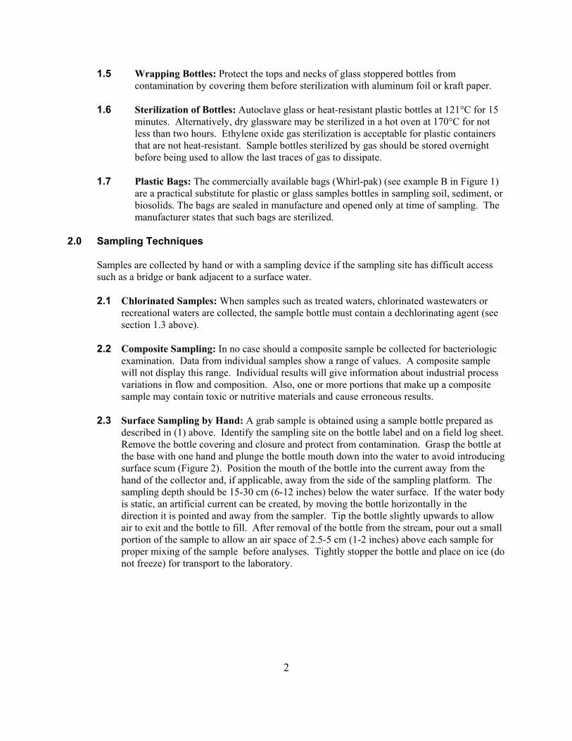
1.5 Wrapping Bottles: Protect the tops and necks of glass stoppered bottles from contamination by covering them before sterilization with aluminum foil or kraft paper.

1.6 Sterilization of Bottles: Autoclave glass or heat-resistant plastic bottles at 121°C for 15 minutes. Alternatively, dry glassware may be sterilized in a hot oven at 170°C for not less than two hours. Ethylene oxide gas sterilization is acceptable for plastic containers that are not heat-resistant. Sample bottles sterilized by gas should be stored overnight before being used to allow the last traces of gas to dissipate.

1.7 Plastic Bags: The commercially available bags (Whirl-pak) (see example B in Figure 1) are a practical substitute for plastic or glass samples bottles in sampling soil, sediment, or biosolids. The bags are sealed in manufacture and opened only at time of sampling. The manufacturer states that such bags are sterilized.

2.0 Sampling Techniques

Samples are collected by hand or with a sampling device if the sampling site has difficult access such as a bridge or bank adjacent to a surface water.

2.1 Chlorinated Samples: When samples such as treated waters, chlorinated wastewaters or recreational waters are collected, the sample bottle must contain a dechlorinating agent (see section 1.3 above).

2.2 Composite Sampling: In no case should a composite sample be collected for bacteriologic examination. Data from individual samples show a range of values. A composite sample will not display this range. Individual results will give information about industrial process variations in flow and composition. Also, one or more portions that make up a composite sample may contain toxic or nutritive materials and cause erroneous results.

2.3 Surface Sampling by Hand: A grab sample is obtained using a sample bottle prepared as described in (1) above. Identify the sampling site on the bottle label and on a field log sheet. Remove the bottle covering and closure and protect from contamination. Grasp the bottle at the base with one hand and plunge the bottle mouth down into the water to avoid introducing surface scum (Figure 2). Position the mouth of the bottle into the current away from the hand of the collector and, if applicable, away from the side of the sampling platform. The sampling depth should be 15-30 cm (6-12 inches) below the water surface. If the water body is static, an artificial current can be created, by moving the bottle horizontally in the direction it is pointed and away from the sampler. Tip the bottle slightly upwards to allow air to exit and the bottle to fill. After removal of the bottle from the stream, pour out a small portion of the sample to allow an air space of 2.5-5 cm (1-2 inches) above each sample for proper mixing of the sample before analyses. Tightly stopper the bottle and place on ice (do not freeze) for transport to the laboratory.

2

Figure 2. Grab sampling technique for surface waters.

3.0 Selection of Sampling Sites and Frequency

These will be described for streams, rivers, estuarine, marine, and recreational waters as well as domestic and industrial wastewaters.

3.1 Stream Sampling: The objectives of the initial survey dictate the location, frequency and number of samples to be collected.

3.1.1 Selection of Sampling Sites: A typical stream sampling program includes sampling locations upstream of the area of concern, upstream and downstream of waste discharges, upstream and downstream from tributary entrances to the river and upstream of the mouth of the tributary. For more complex situations, where several waste discharges are involved, sampling includes sites upstream and downstream from the combined discharge area and samples taken directly from each industrial or municipal waste discharge. Using available bacteriological, chemical and discharge rate data, the contribution of each pollution source can be determined.

3.1.2 Small Streams: Small streams should be sampled at background stations upstream of the pollution sources and at stations downstream from pollution sources. Additional sampling sites should be located downstream to delineate the zones of pollution. Avoid sampling areas where stagnation may occur (e.g., backwater of a tributary) and areas located near the inside bank of a curve in the stream which may not be representative of the main channel.

3

3.1.3 Large Streams and Rivers: Large streams are usually not well mixed laterally for long distances downstream from the pollution sources. Sampling sites below point source pollution should be established to provide desired downstream travel time and dispersal as determined by flow rate measurements. Particular care must be taken to establish the proper sampling points. Occasionally, depth samples are necessary to determine vertical mixing patterns.

3.2 Estuarine and Marine Sampling: Sampling estuarine and marine waters requires the consideration of other factors in addition to those usually recognized in fresh water sampling. They include tidal cycles, current patterns, bottom currents and counter-currents, stratification, seasonal fluctuations, dispersion of discharges and multi-depth samplings.

The frequency of sampling varies with the objectives. When a sampling program is started, it may be necessary to sample every hour around the clock to establish pollution loads and dispersion patterns. The sewage discharges may occur continuously or intermittently.

When the sampling strategy for a survey is planned, data may be available from previous hydrological studies done by the Coast Guard, Corps of Engineers, National Oceanic and Atmospheric Administration (NOAA), U.S. Geological Survey, or university and private research investigations. In a survey, float studies and dye studies are often carried out to determine surface and undercurrents. Initially depth samples are taken on the bottom and at five feet increments between surface and bottom. A random grid pattern for selecting sampling sites is established statistically.

3.2.1 Estuarine Sampling: When a survey is made on an estuary, samples are often taken from a boat, usually making an end to end traverse of the estuary. Another method involves taking samples throughout a tidal cycle, every hour or two hours from a bridge or from an anchored boat at a number of fixed points.

In a large bay or estuary where many square miles of area are involved, a grid or series of stations may be necessary. Two sets of samples are usually taken from an area on a given day, one at ebb or flood slack water, and the other three hours earlier, or later, at the half tidal interval. Sampling is scheduled so that the mid-sampling time of each run coincides with the calculated occurrence of the tidal condition.

In location sampling sites, one must consider points at which tributary waters enter the main stream or estuary, location of shellfish beds and bathing beaches. The sampling stations can be adjusted as data accumulate. For example, if a series of stations half mile apart consistently show similar values, some of these stations may be dropped and other stations added in areas where data shows more variability.

Considerable stratification can occur between the salt water from the sea and the fresh water supplied by a river. It is essential when starting a survey of an unknown estuary to find out whether there is any marked stratification. This can be done by chloride determinations at different locations and depths. It is possible for stratification to occur in one part of an estuary and not in another.

4

On a flood tide, the more dense salt water pushing up into the less dense fresh river water will cause an overlapping with the fresh water flowing on top. A phenomenon called a salt water wedge can form. As a result, stratification occurs. If the discharge of pollution is in the salt water layer, the contamination will be concentrated near the bottom at the flood tide. The flow or velocity of the fresh water will influence the degree of stratification which occurs. If one is sampling only at the surface, it is possible that the data will not show the polluted underflowing water which was contaminated at the point below the fresh water river. Therefore, where stratification is suspected, samples at different depths will be needed to measure vertical distribution.

3.2.2 Marine Sampling: In ocean studies, the environmental conditions are most diverse along the coast where shore, atmosphere and the surf are strong influences. The shallow coastal waters are particularly susceptible to daily fluctuations in temperature and seasonal changes.

Sampling during the entire tidal cycle or during a half cycle may be required. Many ocean studies such as sampling over the continental shelf involve huge areas and no two areas of water are the same.

Selection of sampling sites and depths are most critical in marine waters. In winter, cooling of coastal waters can result in water layers which approach 0°C. In summer, the shallow waters warm much faster than the deeper waters. Despite the higher temperature, oxygen concentrations are higher in shallow than in deeper waters due to greater water movement, surf action and photosynthetic activity from macrophytes and the plankton.

Moving from the shallow waters to the intermediate depths, one observes a moderation of these shallow water characteristics. In the deeper waters, there is a marked stabilization of conditions. Water temperatures are lower and more stable. There is limited turbulence, little penetration of light, sparse vegetation and the ocean floor is covered with a layer of silts and sediments.

3.3 Recreational Waters (Bathing Beaches): Sampling sites at bathing beaches or other recreational areas should include upstream or peripheral areas and locations adjacent to natural drains that would discharge stormwater, or run-off areas draining septic wastes from restaurants, boat marinas, or garbage collection areas. Samples of bathing beach water should be collected at locations and times of heaviest use. Daily sampling, preferably in the afternoon, is the optimum frequency during the season. Weekends and holidays which are periods of highest use must be included in the sampling program. Samples of estuarine bathing waters should be obtained at high tide, ebb tide and low tide in order to determine the cyclic water quality and deterioration that must be monitored during the swimming season.

5

3.4 Domestic and Industrial Waste Discharges: It is often necessary to sample secondary and tertiary wastes from municipal waste treatment plants and various industrial waste treatment operations. In situations where the plant treatment efficiency varies considerably, grab samples are collected around the clock at selected intervals for a three to five day period. If it is known that the process displays little variation, fewer samples are needed. In no case should a composite sample be collected for bacteriological examination. The National Pollution Discharge Elimination System (NPDES) has established wastewater treatment plant effluent limits for all dischargers. These are often based on maximum and mean values. A sufficient number of samples must be collected to satisfy the permit and/or to provide statistically sound data and give a fair representation of the bacteriological quality of the discharge.

6

Appendix B:Part II (General Operations), Sections C.3.5 (Counting Colonies)

and C.3.6 (Calculation of Results)

Counting Colonies1

1.0 Counting Colonies

Colonies should be counted using a fluorescent lamp with a magnifying lens. The flourescent lamp should be nearly perpendicular to the membrane filter. Count colonies individually, even if they are in contact with each other. The technician must learn to recognize the difference between two or more colonies which have grown into contact with each other and single, irregularly shaped colonies which sometimes develop on membrane filters. The latter colonies are usually associated with a fiber or particulate material and the colonies conform to the shape and size of the fiber or particulates. Colonies which have grown together almost invariably show a very fine line of contact.

2.0 Calculation of Results

2.1 Select the membrane filter with the number of colonies in the acceptable range and calculate count per 100 mL according to the general formula:

Count per 100 mL = (No. of colonies counted/Volume of sample filtered, in mL) x 100

2.2 Counts Within the Acceptable Limits

The acceptable range of colonies that are countable on a membrane is a function of the method. Different methods may have varying acceptable count ranges. All examples in this appemdix assume that the acceptable range of counts is between 20-60 colonies per membrane.

For example, assume that filtration of volumes of 50, 15, 5, 1.5, and 0.5 mL produced colony counts of 200, 110, 40, 10, and 5, respectively.

An analyst would not actually count the colonies on all filters. By inspection the analyst would select the membrane filter with the acceptable range of target colonies, as defined by the method, and then limit the actual counting to such membranes.

After selecting the best membrane filter for counting, the analyst counts colonies and applies the general formula as in section 2.1 above to calculate the count/100 mL.

2.3 More Than One Acceptable Count

2.3.1 If there are acceptable counts on replicate plates, carry counts independently to final reporting units, then calculate the arithmetic mean of these counts to obtain the final reporting value.

1The text is largely taken from Part II, Section C, of the EPA publication "Microbiological Methods for Monitoring the Environment" EPA-600/8-78-017, December 1978. Some examples were kindly provided by Kristen Brenner, US EPA.

1

Example, if the counts are 24 and 36 for replicate plates of 100 mL each, then the arithmetic mean is calculated as follows:

(24 CFU/100 mL + 36 CFU/100 mL) = 30 CFU/ 100 mL

2

2.3.2 If there is more than one dilution having an acceptable range of counts, independently carry counts to final reporting units, then average for final reported value.

For example, if volumes of 100, 10, 1 and 0.1 mL produced colony counts of Too Numerous To Count (TNTC), 55, 30, and 1, respectively, then two volumes, 10 mL and 1 mL, produced colonies in the acceptable counting range.

Independently carry each MF count to a count per 100 mL:

55 × 100 = 550 CFU /100 mL

10

and

30 × 100 = 3000 CFU /100 mL

1

Calculate the arithmetic mean as in section 2.3.1 above:

(550 CFU/100 mL + 3000 CFU/100 mL) = 1775 CFU/100 mL

2

Report this as 1775 CFU/100 mL.

2.4 If all MF counts are below the lower acceptable count limit, select the most nearly acceptable count.

2.4.1 For example, sample volumes of 100, 10 and 1 mL produced colony counts of 17, 1 and 0, respectively.

Here, no colony count falls within recommended limits. Calculate on the basis of the most nearly acceptable plate count, 17, and report as 17 CFU/100 mL.

Note that in this case, because no calculations were done (i.e. this is the count for 100 mL), the count is reported as 17 CFU/100 mL rather than an “estimated count of 17 CFU/100 mL”

2

2.4.2 As a second example, assume a count in which sample volumes of 10 and 1 mL produced colony counts of 18 and 0, respectively.

Here, no colony count falls within recommended limits. Calculate on the basis of the most nearly acceptable plate count, 18, and calculate as in section 2.3.2 above.

18 × 100 = 180 CFU /100 mL

10

Report this as an estimated count of 180 CFU/100 mL.

2.5 If counts from all membranes are zero, calculate using count from largest filtration volume.

For example, sample volumes of 25, 10, and 2 mL produced colony counts of 0, 0, and 0, respectively, and no actual calculation is possible, even as an estimated report. Calculate the number of colonies per 100 mL that would have been reported if there had been one colony on the filter representing the largest filtration volume. In this example, the largest volume filtered was 25 mL and thus the calculation would be:

1 × 100 = 4 CFU /100 mL

25

Report this as < (less than) 4 CFU/100 mL.

2.6 If all membrane counts are above the upper acceptable limit, calculate count using the smallest volume filtered.

For example, assume that the volumes 1, 0.3, and 0.01 mL produced colony counts of TNTC, 150, and 110 colonies, respectively. Since all colony counts are above the acceptable limit, use the colony count from the smallest sample volume filtered and estimate the count as:

110 × 100 = 1,100,000 CFU /100 mL

0.01

Report this as estimated count 1.1 × 106 CFU/100 mL

2.7 If typical colonies are too numerous to count (TNTC), use upper limit count with smallest filtration volume.

3

For example, assume that the volumes 1, 0.3, and 0.01 mL all produced too many typical colonies, and that the laboratory bench record indicated TNTC.

Use the upper acceptable count for the method (60 colonies in this example) as the basis of calculation with the smallest filtration volume and estimate the count as:

60 × 100 = 600,000 CFU /100 mL

0.01

Report this as > (greater than) 6 ×105 CFU/100 mL

2.8 If colonies are both above and below the upper and lower acceptable limits (i.e., no counts are within the acceptable limits), select the most nearly acceptable count.

2.8.1 For example, sample volumes of 100, 10 and 1 mL produced colony counts of 64, 6 and 0, respectively.

Here, no colony count falls within recommended limits. Calculate on the basis of the most nearly acceptable plate count, 64, and report as 64 CFU/100 mL.

Note that in this case, because no calculations were done (i.e. this is the count for 100 mL), the count is reported as 64 CFU/100 mL rather than an “estimated count of 64 CFU/100 mL”

2.8.2 As a second example, assume a count in which sample volumes of 100, 10 and 1 mL produced colony counts of 98, 18, and 0, respectively.

Here, no colony count falls within recommended limits. Calculate on the basis of the most nearly acceptable plate count, 18, and calculate as in section 2.3.2 above.

18 × 100 = 180 CFU /100 mL

10

Report this as estimated count 180 CFU/100 mL.

2.9 If there is no result because of a confluent growth, > 200 atypical colonies (TNTC), lab accident, etc., report as No Data and specify the reason.

4

Designation: D1253 − 08

StandardTest Method forResidual Chlorine in Water1

This standard is issued under the fixed designation D1253; the number immediately following the designation indicates the year oforiginal adoption or, in the case of revision, the year of last revision. A number in parentheses indicates the year of last reapproval. Asuperscript epsilon (´) indicates an editorial change since the last revision or reapproval.

1. Scope

1.1 This test method covers the determination of residualchlorine in water by direct amperometric titration.

1.2 Within the constraints specified in Section 6, this testmethod is not subject to commonly encountered interferencesand is applicable to most waters. Some waters, however, canexert an iodine demand, usually because of organic material,making less iodine available for measurement by this testmethod. Thus, it is possible to obtain falsely low chlorinereadings, even though the test method is working properly,without the user’s knowledge.

1.3 Precision data for this test method were obtained onestuary, inland main stem river, fresh lake, open ocean, andfresh cooling tower blowdown water. Bias data could not bedetermined because of the instability of solutions of chlorine inwater. It is the user’s responsibility to ensure the validity of thetest method for untested types of water.

1.4 In the testing by which this standard was validated, thedirect and back starch-iodide titrations and the amperometricback titration, formerly part of this standard, were found to beunworkable and were discontinued in 1986. Historical infor-mation is presented in Appendix X1.

NOTE 1—Orthotolidine test methods have been omitted because of poorprecision and accuracy.

1.5 The values stated in SI units are to be regarded asstandard. No other units of measurement are included in thisstandard.

1.6 This standard does not purport to address all of thesafety concerns, if any, associated with its use. It is theresponsibility of the user of this standard to establish appro-priate safety and health practices and determine the applica-bility of regulatory limitations prior to use.

2. Referenced Documents

2.1 ASTM Standards:2

D1129 Terminology Relating to WaterD1193 Specification for Reagent WaterD2777 Practice for Determination of Precision and Bias of

Applicable Test Methods of Committee D19 on WaterD3370 Practices for Sampling Water from Closed ConduitsD5847 Practice for Writing Quality Control Specifications

for Standard Test Methods for Water Analysis

3. Terminology

3.1 Definitions: For definitions of terms used in this testmethod, refer to Terminology D1129.

3.2 Definitions of Terms Specific to This Standard:3.2.1 combined residual chlorine, n—residual consisting of

chlorine combined with ammonia nitrogen or nitrogenouscompounds.

3.2.2 free available chlorine residual, n—residual consist-ing of hypochlorite ions, hypochlorous acid, or a combinationthereof.

3.2.3 total residual chlorine (chlorine residual), n—theamount of available chlorine-induced oxidants present in waterat any specified period, subsequent to the addition of chlorine.

NOTE 2—Chlorine present as chloride is neither included in these termsnor determined by this test method.

NOTE 3—Bromine, bromine combined with ammonia or nitrogenouscompounds, and chlorine dioxide are not distinguished by this test methodfrom the corresponding chlorine compounds.

4. Summary of Test Method

4.1 This is an amperometric titration test method utilizingphenylarsine oxide as the titrant. When the titrator cell isimmersed in a sample containing chlorine, current is generated.As phenylarsine oxide is added, the chlorine is reduced and thegeneration of current ceases. When chlorine is present as achloramine, potassium iodide is added, releasing iodine, which

1 This test method is under the jurisdiction of ASTM Committee D19 on Waterand is the direct responsibility of Subcommittee D19.05 on Inorganic Constituentsin Water.

Current edition approved Oct. 1, 2008. Published October 2008. Originallyapproved in 1953. Last previous edition approved in 2003 as D1253 – 03. DOI:10.1520/D1253-08.

2 For referenced ASTM standards, visit the ASTM website, www.astm.org, orcontact ASTM Customer Service at [email protected]. For Annual Book of ASTMStandards volume information, refer to the standard’s Document Summary page onthe ASTM website.

*A Summary of Changes section appears at the end of this standard

Copyright © ASTM International, 100 Barr Harbor Drive, PO Box C700, West Conshohocken, PA 19428-2959. United States

NOTICE: This standard has either been superseded and replaced by a new version or withdrawn.Contact ASTM International (www.astm.org) for the latest information

1

Copyright by ASTM Int'l (all rights reserved); Wed Dec 3 15:52:49 EST 2014Downloaded/printed byKrish Ramalingam (The City College of New York - Department of Civil Engineering) pursuant to License Agreement. No further reproductions authorized.

http://dx.doi.org/10.1520/D1129







http://www.astm.org/COMMIT/COMMITTEE/D19.htm

http://www.astm.org/COMMIT/SUBCOMMIT/D1905.htm

is titrated in a similar manner. The iodine content is calculatedin terms of free chlorine.

5. Significance and Use

5.1 Chlorine is used to destroy or deactivate a variety ofunwanted chemicals and microorganisms in water and waste-water.

5.2 An uncontrolled excess of chlorine in water, whetherfree available or combined, can adversely affect the subsequentuse of the water.

6. Interferences

6.1 This test method is not subject to interferences fromtemperature, color, or turbidity of sample.

6.2 Values of pH above 8.0 interfere by slowing the reactionrate. Buffering the sample to pH 7.0 or less eliminates theinterference.

6.3 Erratic behavior of the apparatus in the presence ofcupric ions has been reported.

6.4 Cuprous and silver ions tend to poison the electrode ofthe titrator.

6.5 Nitrogen trichloride and some N-chloro compounds areoften present as products of the chlorination of wastewatersand will titrate partially as free available chlorine and partiallyas combined residual chlorine. This error can be avoided onlyin the determination of total residual chlorine.

6.6 Exposure to high concentrations of free available chlo-rine causes a film-type polarization that reverses very slowly.

This can be avoided by diluting the sample with water to lessthan 10 mg/L of free available chlorine.

6.7 If chlorine dioxide is present, an unknown portiontitrates as free available chlorine. Total chlorine dioxide titratesas total residual chlorine.

6.8 Depending upon final pH, chlorination of waters con-taining ammonia or nitrogenous organic compounds can pro-duce high concentrations of dichloramine. This compoundproduces four to five times as much current as monochloram-ine. The current produced by as little as 5 mg/L of dichloram-ine can cause the microammeter pointer to read offscale even atthe end point in the titration of free available chlorine. Thismay be overcome by use of an opposing voltage in theapparatus’ circuitry. The instrument’s manufacturer should beconsulted in this regard.

7. Apparatus

7.1 Amperometric Titration Apparatus3,4—Refer to Fig. 1.

NOTE 4—When the titrator has been out of service for a day or more,check the electrode for sensitivity by noting the rapidity of the pointerdeflection. If the pointer responds slowly after the addition of KI solution,add a small amount of biiodate. If it responds slowly to free availablechlorine, sensitize it by adding chlorine.

3 Water and Sewage Works, May 1949, p. 171, and Journal American WaterWorks Association, Vol 34, 1942, pp. 1227–1240.

4 Amperometric titrators are available commercially from most laboratory supplyhouses.

FIG. 1 Wiring Diagram of Amperometric Titrator

D1253 − 08

2


7.2 Glassware—Condition with water containing at least 10mg/L of residual chlorine for at least 2 h prior to use and thenrinse thoroughly.

8. Reagents and Materials

8.1 Purity of Reagents—Reagent grade chemicals shall beused in all tests. Unless otherwise indicated, it is intended thatall reagents shall conform to the specifications of the Commit-tee on Analytical Reagents of the American Chemical Society.5

Other grades may be used, provided it is first ascertained thatthe reagent is of sufficiently high purity to permit its usewithout lessening the accuracy of the determination.

8.2 Purity of Water—Unless otherwise indicated, referencesto water shall be understood to mean reagent water conformingto Specification D1193, Type III, further treated to be free ofchlorine demand. Other reagent water types (Type I) may beused provided it is first ascertained that the water is ofsufficiently high purity to permit its use without adverselyaffecting the bias and precision of the test method. Type IIIwater was specified at the time of round robin testing of thismethod. A suggested method for preparation of chlorinedemand-free water is to add approximately 20 mg/L ofavailable chlorine to Type III water, let it stand for about aweek in darkness, and then expose it to sunlight until nochlorine remains. Filtration through a carbon filter is analternative process which requires less time to remove chlo-rine.

8.3 pH 4.0 Buffer Solution—Dissolve 243 g of sodiumacetate trihydrate and 480 g of glacial acetic acid in water anddilute to 1 L.

8.4 pH 7.0 Buffer Solution—Dissolve 25.4 g of monobasicpotassium phosphate and 86 g of dibasic sodium phosphate inwater and dilute to 1 L.

8.5 Biiodate, Solution Standard (0.0282N)—Dissolve0.9163 g of potassium biiodate in water and dilute to 1 L in avolumetric flask. Store in an amber glass-stoppered bottle.

8.6 Phenylarsine Oxide, Solution Standard (0.00564 N)—Dissolve 0.8 g of phenylarsine oxide in 150 mL of sodiumhydroxide solution (12 g/L). After settling, decant 110 mL ofthis solution, add 800 mL of water, and bring to a pH of 9.0 byadding hydrochloric acid (1 + 1). This should require about 2mL of HCl (1 + 1). Continue acidification with HCl (1 + 1)until a pH of 6 to 7 is reached, as indicated by a glass-electrodesystem; then dilute to a total volume of 1L. Standardize to0.00564 N against 0.0282 N biiodate solution using the titrator(7.1) as the end-point indicator. Add 1 mL of chloroform forpreservation.

8.7 Potassium Iodide Solution (50 g/L)—Dissolve 50 g ofKI in water and dilute to 1 L. Add 1 g of sodium bicarbonate

to stabilize the solution. Store in an amber bottle and avoiddirect exposure to sunlight.

9. Sampling

9.1 Collect the sample in accordance with Practices D3370.Take care that the sample is representative and keep it awayfrom direct sunlight prior to analysis.

9.2 All tests should be made as soon as possible aftercollection of the sample (not more than 5 min) because theresidual chlorine may diminish with time, due to the chlorinedemand of the sample. Where time of contact is important, theelapsed time between the addition of chlorine and the deter-mination of chlorine should be taken into account.

10. Procedure

10.1 For residual chlorine concentrations of 2.0 mg/L orless, use a 200-mL sample. For greater concentrations, use a100-mL sample. It is preferable that the size of the sample besuch that not more than 2 mL of titrant will be required tocomplete the titration.

10.2 Determination of Total Residual Chlorine:10.2.1 Add 1 mL of KI solution to a 200-mL sample and

immediately add 1 mL of pH 4.0 buffer solution.10.2.2 Immerse the electrodes in the sample and start the

stirrer. Adjust the microammeter pointer of the potentiometerto the right or high current side of the scale so the pointer candeflect counterclockwise during the analysis.

10.2.3 Titrate using standard phenylarsine oxide solution,adding the titrant in small increments, and noting the deflectionof the microammeter pointer. Plot the progress of the titrationon linear graph paper with current on the vertical axis andtitrant volume on the horizontal axis. Add a small volume oftitrant, wait a few seconds, and plot the current-volume pointon the graph.

10.2.4 Readjust the potentiometer several times during thetitration, if necessary, to bring the pointer back on scale.

10.2.5 Continue the analysis by determining at least threepoints spread over the downward sloping titration curve and atleast three points after the equivalence or end point. The latterpoints will indicate practically no change in current. Points justbefore the end point shall be disregarded in its determination.The millilitres of titrant at the end point defined by theintersection of the two linear sections of the titration curveshould be recorded.

10.3 Determination of Free Available Chlorine Residual:10.3.1 Add 1 mL of pH 7.0 buffer solution to a 200-mL

sample.10.3.2 Repeat the phenylarsine oxide titration beginning

with 10.2.2.10.3.3 Note a rapid deflection of the pointer for each

increment of titrant indicates the presence of free availablechlorine. Slight counterclockwise movements of the pointerafter addition of individual drops of titrant is a drift effect anddoes not indicate the presence of free available chlorine.

10.4 Determination of Combined Available Chlorine Re-sidual:

5 Reagent Chemicals, American Chemical Society Specifications, AmericanChemical Society, Washington, DC. For Suggestions on the testing of reagents notlisted by the American Chemical Society, see Annual Standards for LaboratoryChemicals, BDH Ltd., Poole, Dorset, U.K., and the United States Pharmacopeiaand National Formulary, U.S. Pharmacopeial Convention, Inc. (USPC), Rockville,MD.

D1253 − 08

3


10.4.1 Complete the titration for the determination of freeavailable chlorine residual as in 10.3.

10.4.2 To the same sample, add 1 mL of KI solution and 1mL of pH 4.0 buffer solution and repeat the titration as in 10.2.

11. Calculation

11.1 Calculate the various types of chlorine residual, inmilligrams per litre, as follows:

Chlorine residual, mg/L 5 200 A/V

where:A = phenylarsine oxide solution (0.00564 N) required for

the titration of 10.2, 10.3, or 10.4, depending on thespecific type of chlorine residual determined, mL, and

V = sample used, mL.

12. Precision and Bias6

12.1 The overall precision (St) and the single operatorprecision (So) of this test method for free available chlorine(FAC) and for total residual chlorine (TRC) were determinedby eight or nine qualified cooperators each with analysisequipment and reagents at each of five sites. Each siteconstituted a different chlorinated cooling water matrix:estuary, inland main stem river, fresh lake, open ocean, andfresh cooling tower blowdown. Each site water was chlorinatedup to nine levels. Samples were collected simultaneously andanalyzed within 5 min of collection by all eight or ninecooperators. Duplicate sampling and analysis runs were madeat each level.

12.2 The St and So for FAC was found to vary linearly withthe mean concentration of FAC, X, in mg/L, over the range forX from 0.0 to 1.0.

12.2.1 For the pooled results from all of the matrices tested:

S t 5 0.02510.199 X ~n 5 37, r 5 0.848!

So 5 0.00810.081 X ~n 5 35, r 5 0.638!

where:n = number of runs, andr = correlation coefficients.

12.3 The St and So for TRC was found to vary linearly withthe mean concentration of TRC, Y, in mg/L, over the range forY from 0.0 to 3.5.

12.3.1 For the pooled results from all of the matrices tested:

St 5 0.02210.098 Y ~n 5 39, r 5 0.865!

So 5 0.01210.024 Y ~n 5 38, r 5 0.695!

12.4 The bias of the test method could not be determinedsince the instability of solutions of chlorine in water does notpermit the determination of an acceptable true value for TRCand FAC in the samples.

12.5 Precision for this test method conforms to PracticeD2777 – 77, which was in place at the time of collaborativetesting. Under the allowances made in 1.4 of Practice

D2777 – 06, these precision data do meet existing require-ments for interlaboratory studies of Committee D19 testmethods.

13. Quality Control

13.1 In order to be certain that analytical values obtainedusing these test methods are valid and accurate within theconfidence limits of the test, the following QC procedures shallbe followed when analyzing residual chlorine.

13.2 Calibration and Calibration Verification:13.2.1 Standardize the titrating solution against the potas-

sium biiodate solution.13.2.2 Verify titrating solution by analyzing a sample with a

known amount of the residual chlorine. The amount of thesample shall fall within 615 % of the known concentration.

13.2.3 If standardization cannot be verified, restandardizethe solution.

13.3 Initial Demonstration of Laboratory Capability:13.3.1 If a laboratory has not performed the test before, or if

there has been a major change in the measurement system, forexample, new analyst, new instrument, and so forth, a precisionand bias study shall be performed to demonstrate laboratorycapability.

13.3.2 Analyze seven replicates of a known solution pre-pared from an Independent Reference Material containing aknown amount of residual chlorine. Each replicate shall betaken through the complete analytical test method includingany sample preservation and pretreatment steps. The replicatesmay be interspersed with samples.

13.3.3 Calculate the mean and standard deviation of theseven values and compare to the acceptable ranges of bias inSection 12. This study should be repeated until the recoveriesare within the limits given in Section 12. If an amount otherthan the recommended amount is used, refer to Practice D5847for information on applying the F test and t test in evaluatingthe acceptability of the mean and standard deviation.

13.4 Laboratory Control Sample (LCS):13.4.1 To ensure that the test method is in control, analyze

an LCS containing a known amount of residual chlorine witheach batch or 10 samples. If large numbers of samples areanalyzed in the batch, analyze the LCS after every ten samples.The LCS shall be taken through all of the steps of the analyticalmethod including sample preservation and pretreatment. Theresult obtained for the LCS shall fall within 615 % of theknown amount.

13.4.2 If the result is not within these limits, analysis ofsamples is halted until the problem is corrected and either allthe samples in the batch must be reanalyzed, or the results mustbe qualified with an indication that they do not fall within theperformance criteria of the test method.

13.5 Method Blank:13.5.1 Analyze a reagent water test blank with each batch.

The amount of residual chlorine found in the blank should beless than the analytical reporting limit. If the amount ofresidual chlorine is found above this level, analysis of samplesis halted until the contamination is eliminated, and a blankshows no contamination at or above this level, or the results

6 Supporting data have been filed at ASTM International Headquarters and maybe obtained by requesting Research Report RR:D19-1124. Contact ASTM CustomerService at [email protected].

D1253 − 08

4


shall be qualified with an indication that they do not fall withinthe performance criteria of the test method.

13.6 Matrix Spike (MS):

13.6.1 Residual chlorine is not an analyte that can befeasibly spiked into samples.

13.7 Duplicate:

13.7.1 To check the precision of sample analyses, analyze asample in duplicate with each batch. The value obtained shallfall within the control limits established by the laboratory.

13.7.2 Calculate the standard deviation of the duplicatevalues and compare to the precision in the collaborative studyusing an F test. Refer to 6.4.4 of Practice D5847 for informa-tion on applying the F test.

13.7.3 If the result exceeds the precision limit, the batchshall be reanalyzed or the results shall be qualified with anindication that they do not fall within the performance criteriaof the test method.

13.8 Independent Reference Material (IRM):13.8.1 In order to verify the quantitative value produced by

the test method, analyze an Independent Reference Material(IRM) submitted as a regular sample (if practical) to thelaboratory at least once per quarter. The amount of the IRMshould be in the analytical range for the method chosen. Thevalue obtained shall fall within the control limits established bythe laboratory.

14. Keywords

14.1 amperometric; analysis; chlorine; water

APPENDIX

(Nonmandatory Information)

X1. RATIONALE FOR DISCONTINUATION OF TEST METHODS

X1.1 Direct and Back Starch-Iodide Titrations and Ampero-metric Back Titration:

X1.1.1 These two test methods were discontinued in 1986.These test methods may be found in 1985 Annual Book ofASTM Standards, Vol 11.01. These test methods were origi-nally issued in 1953.

X1.1.2 These test methods are biiodate solutions as titratingagents. Attempts to include these test methods in the round-robin testing were not successful because the reaction rate of

the biiodate solution with phenylarsine oxide was slow andinconsistent. The little data obtained were widely varied,nonreproducible, and were not relatable to the values beingtested.

X1.1.3 Field experience indicates that both test methods canwork if iodine solution is used in place of biiodate solution asthe titrating agent. Validation of these test methods throughround-robin testing, however, has not been carried out.

ASTM International takes no position respecting the validity of any patent rights asserted in connection with any item mentionedin this standard. Users of this standard are expressly advised that determination of the validity of any such patent rights, and the riskof infringement of such rights, are entirely their own responsibility.

This standard is subject to revision at any time by the responsible technical committee and must be reviewed every five years andif not revised, either reapproved or withdrawn. Your comments are invited either for revision of this standard or for additional standardsand should be addressed to ASTM International Headquarters. Your comments will receive careful consideration at a meeting of theresponsible technical committee, which you may attend. If you feel that your comments have not received a fair hearing you shouldmake your views known to the ASTM Committee on Standards, at the address shown below.

This standard is copyrighted by ASTM International, 100 Barr Harbor Drive, PO Box C700, West Conshohocken, PA 19428-2959,United States. Individual reprints (single or multiple copies) of this standard may be obtained by contacting ASTM at the aboveaddress or at 610-832-9585 (phone), 610-832-9555 (fax), or [email protected] (e-mail); or through the ASTM website(www.astm.org). Permission rights to photocopy the standard may also be secured from the ASTM website (www.astm.org/COPYRIGHT/).

D1253 − 08

5


Attachment 3

Ambient TRC Bench

Scale Studies

PROPOSAL TO

NEW YORK DEPARTMENT OF ENVIRONMENTAL PROTECTION

FOR

Chlorine DEGRADATION STUDIES FOR TWO NYC DEP CSO

FACILITIES

Prepared by:

Great Lakes Environmental Center, Inc.

739 Hastings Street

Traverse City, MI 49686

In collaboration with

Manhattan College

Principal Contact Persons:

Mick DeGraeve

[email protected]

Phone: (231) 941-2230

Rob Sharp

[email protected]

Phone: (917)226-9377)

June 18, 2015

mailto:[email protected]

mailto:[email protected]

2

Brief Description of Planned CSO Degradation Studies

Receiving Water and CSO Samples

CSO-specific receiving water samples will be collected using GLEC equipment and will be

hauled from the receiving water of interest to the GLEC mobile laboratory currently housed at

26th

Ward WWTP, where the samples will be off-loaded into a storage tank. The CSO samples

will be collected during a rain event using GLEC equipment, and will also be hauled to the

GLEC mobile lab at the 26th

Ward WWTP. Prior to any testing, the CSO and receiving water

samples will be characterized for TSS, turbidity, ammonia, nitrite, nitrate and COD, as well as

pH and temperature. In addition, both the effluents and receiving waters will be tested for initial

fecal coliform and enterococcus densities prior to each test.

Chlorine Degradation Studies with Pathogen Inactivation

The CSO chlorine degradation studies will be carried using equipment in the GLEC mobile

laboratory, as well as at space provided by the 26th

Ward in-house laboratory. The studies will

mimic the degradation studies that were developed under the TRC program for DEP in

2013/2014. Between four-six samples will be collected from each of the two selected CSO

facilities during the study. Each sample will be tested for chlorine degradation and pathogen

inactivation at 2 different dilutions and with 3 different applied chlorine doses. The selected

dilutions will be determined in collaboration with DEP based on the specific CSO discharge

location and the hydraulics of the receiving water location. The chlorine doses to be tested will

range between 4 - 20 mg/l ; the specific doses to be tested will be informed by the on-going CSO

disinfection studies. Figure 1 shows the proposed set of testing conditions for a single CSO

sample. These testing conditions will be used to run the collected samples in duplicate over a

two-to-three day period after the CSO sample is collected. Each specific testing condition will

be carried out in a batch system according to the dilution and sampling times shown in Figure 2.

Figure 1 – Degradation Testing Conditions

Cl Dose 1

Cl Dose 2

Cl Dose 3

Dilution 1 Dilution 2

3

Figure 2 – CSO Chlorine Degradation Test with Specific Dilution and Sampling Times

The specific analyses that will be carried on each sample are shown in Table 1. CPO represents

chemically-(chlorine) produced oxidant, which is how free and combined chlorine are measured

using standard methods for wastewaters. EC/FC represents fecal coliform and Entercoccus

counts. The Nitrogen series includes ammonia, nitrite and nitrate. The sampling times may be

altered during the testing period to account for new information gained during the study

Table 1- Sampling Plan for Each Individual Degradation Test

Sample CPO FC/EC N Series pH Turb Temp COD UVT

CSO Sample √ √ √ √ √ √ √ √

Receiving

Water Sample √ √ √ √ √ √ √ √

0 min. √ √ √ √ √ √

1 min. √ √

5 min. √ √

10 min. √ √

15 min. √ √ √ √

17 min. √ √

20 min. √ √

30 min. √ √

45 min. √ √

60 min. √ √ √ √ √

CSOSample

Cl2 Dose

Chlorinated CSO

Sample

DilutedChlorinated

CSOSample

Sampling

CSO Tank

15 Minutes

Receiving Water

Mixing Zone

60 minutes

60 minutes

Run 1

Run 2

CSO Tank

Characterized Receiving Water Added To Chlorinated WW to meet DF over 1 hour

15 Minutes

0 15 17 20 30 45 605 10

tsayan

Polygon

tsayan

Polygon

tsayan

Line

tsayan

Text Box

Weir Wall

tsayan

Line