review questions - ees iiest, shibpur
TRANSCRIPT
Review Questions 15
sensitivity, bandv/idth, and accuracy. Finally, various types of control systems were categorized according to the system signals, linearity, and control objectives. Several typical control-system examples were given to illustrate the analysis and design of control systems. Most systems encountered in real life are nonlinear and time-varying to some extent. The concentration on the studies of linear systems is due primarily to the availability of unified and simple-to-understand analytical methods in the analysis and design of linear systems.
REVIEW QUESTIONS
1. List the advantages and disadvantages of an open-loop system.
2. List the advantages and disadvantages of a closed-loop system.
3. Give the definitions of ac and dc control systems.
4. Give the advantages of a digital control system over a continuous-data control system.
5. A closed-loop control system is usually more accurate than an open-loop system. (T)
6. Feedback is sometimes used to improve the sensitivity of a control system.
7. If an open-loop system is unstable, then applying feedback will always improve its stability.
8. Feedback can increase the gain of a system in one frequency range but decrease it in another.
9. Nonlinear elements are sometimes intentionally introduced to a control system to improve its performance.
10. Discrete-data control systems are more susceptible to noise due to the nature of their signals.
Answers to these review questions can be found on this book's companion Web site: www.wiley.com/college/golnaraghi.
(T) (T)
(T)
(T)
(T)
(T)
(F) (F)
(F)
(F)
(F)
(F)

CHAPTER
Mathematical Foundation
The studies of control systems rely to a great extent on applied mathematics. One of the major purposes of control-system studies is to develop a set of analytical tools so that the designer can arrive with reasonably predictable and reliable designs without depending solely on the drudgery of experimentation or extensive computer simulation.
In this chapter, it is assumed that the reader has some level of familiarity with these concepts through earlier courses. Elementary matrix algebra is covered in Appendix A. Because of space limitations, as well as the fact that most subjects are considered as review material for the reader, the treatment of these mathematical subjects is not exhaustive. The reader who wishes to conduct an in-depth study of any of these subjects should refer to books that are devoted to them.
The main objectives of this chapter are:
1. To introduce the fundamentals of complex variables.
2. To introduce frequency domain analysis and frequency plots.
3. To introduce differential equations and state space systems.
4. To introduce the fundamentals of Laplace transforms.
5. To demonstrate the applications of Laplace transforms to solve linear ordinary differential equations.
6. To introduce the concept of transfer functions and how to apply them to the modeling of linear time-invariant systems.
7. To discuss stability of linear time-invariant systems and the Routh-Hurwitz criterion.
8. To demonstrate the MATLAB tools using case studies.
1A COMPLEX-VARIABLE CONCEPT
To understand complex variables, it is wise to start with the concept of complex numbers and their mathematical properties.
2-1-1 Complex Numbers
A complex number is represented in rectangular form as
Z = x + jy (2-1)
where, j = \/—T and (x, >') are real and imaginary coefficients of z respectively. We can treat (x, y) as a point in the Cartesian coordinate frame shown in Fig. 2-1. A point in a

2-1 Complex-Variable Concept < 17
Imaginary
s-plane
:=x+jy
-•Real
JH Z* = x -jy Figure 2-1 Complex number r representation in rectangular and polar forms.
(2-2)
rectangular coordinate frame may also be defined by a vector R and an angle 6. It is then easy to see that
x = R cos 9
y = R sin 0
where,
R = magnitude of z 9 — phase of z and is measured from the x axis. Right-hand rule convention:
positive phase is in counter clockwise direction. Hence,
R = \ / ^ + . v 2
c ^ t a n - 1 -v
(2-3)
Introducing Eq. (2-2) into Eq. (2-1), we get
z = RcosO + jRsmO (2-4)
Upon comparison of Taylor series of the terms involved, it is easy to confirm
eJe -Rcos0 + sin9 (2-5)
Eq. (2-5) is also known as the Euler formula. As a result, Eq. (2-1) may also be represented in polar form as
z = Rej0 = R16 (2-6)
We define the conjugate of the complex number z in Eq. (2-1) as
z* =x- jy Or, alternatively,
z* = Rcos9- jRsm9 = Re~j0
Note:
Table 2-1 shows basic mathematical properties of complex numbers.
(2-7)
(2-8)
(2-9)

18 Chapter 2. Mathematical Foundaton
TABLE 2-1 Basic Properties of Complex Numbers
Addition
Subtraction
Multiplication
Division
JZ) =-V| +./V] \ Z2 = ^2 + j}'2 -*z = (x\ +x2) + i(.vi + yi)
\z.\ = X\ + j}>] \ zi = X2 + jyi -*Z = (.tl + X2) - /(>'! + V2)
fz\ =-V| +y>'i {Z2= X2 + /V'2 -»z - f>i*2 - V1.V2) - y(xiv2 + -V2.V1)
/ = -1
J si = .v-| + yvi
[ Z2 = -¾ + j}'2
\ z\ = *i - y>'i < Complex Conjugate ( zl = x2 - jyi
_ Z]
Z.2 _ Z\ Z2 _ (X\X2 + V1V2) + j(x\V2 +X2V1 )
zi z2 x$ + y2
Ui^Riei* \z2 = R2eJ02
^z={Rl+R2)eJi^02)
-*z-(Ri +R2)/(9\ +02)
fzi=Rt*t* \z2 = R->ejl'2
- 7 . = ( ^ , - ^ 2 ) ^ ^ - ^ ) -^z=(Rl'R2)/(el-62)
(zi=Rie^ \ 2 2 = / ? 2 ^ -.z=(RiR2y
{e<+0-)
^z=(RiR2)l(9i+e2)
r«i =/?i«>tf|
\ -2 = / ? 2 ^" 2
_»,-- f£/ufe'-^ - w - * - ( * ) * < * - * >
EXAMPLE 2-1-1 F i n d / a n d / .
EXAMPLE 2-1-2 Find z" using Eq. (2-6).
j = V - l = c o s - + . / s i n - = e*i
/ = eJ'2 = e -'2
/ = / 7 = - / = 1
z» = (Rei9)n=R"eJ"f) = R"ln< (2-10)
2-1-2 Complex Variables
A complex variable s has two components: a real component a and an imaginary component co. Graphically, the real component of s is represented by a CT axis in the horizontal direction, and the imaginary component is measured along the vertical jw axis, in the complex .y-planc. Fig. 2-2 illustrates the complex .v-plane, in which any arbitrary point s = ,9| is defined by the coordinates a = o\, and co = co\, or simply Jl = CTl + JCO].

2-1 Complex-Variable Concept 19
j<o s-piane
,v, = a, +j<a]
> a
Figure 2-2 Complex .s-plane.
2-1-3 Functions of a Complex Variable
The function G(.v) is said to be a function of the complex variable s if, for every value of s, there is one or more corresponding values of G(s). Because s is defined to have real and imaginary parts, the function G(s) is also represented by its real and imaginary parts; that is,
G{s)=Re[G{s)] + j\m[G(s)] (2-11)
where Re[G(.s)] denotes the real part of G(.v), and Im[G(.s-)] represents the imaginary part of GO?). The function G(s) is also represented by the complex G(.v)-plane, with Re[G(.?)] as the real axis and Im[G(.v)] as the imaginary axis. If for every value of s there is only one corresponding value of G(s) in the G(.y)-plane, G(s) is said to be a single-valued function, and the mapping from points in the .s-plane onto points in the G(.v)-plane is described as single-valued (Fig. 2-3). If the mapping from the G(tf)-plane to the s-plane is also single-valued, the mapping is called one-to-one. However, there are many functions for which the mapping from the function plane to the complex-variable plane is not single-valued. For instance, given the function
G ( j ) = T - 7 n (2-12) SIS 1
j&
s-plane cox
.s, = (7, +jo)]
*. _
j ImG
G(.v)-plane
i ReC
*-J G(.v,)
Figure 2-3 Single-valued mapping from the s-plane to the Gf.v)-plane.

20 Chapter 2. Mathematical Foundation
it is apparent that, for each value of s, there is only one unique corresponding value for G(s). However, the inverse mapping is not true; for instance, the point G(s) = oo is mapped onto two points, ,v = 0 and s = —1, in the .y-plane.
2-1-4 Analytic Function
A function G(s) of the complex variable s is called an analytic functionin a region of the s-plane if the function and all its derivatives exist in the region. For instance, the function given in Eq. (2-12) is analytic at every point in the s-plane except at the points s — 0 and s = —1. At these two points, the value of the function is infinite. As another example, the function G(s) = s + 2 is analytic at every point in the finite s-plane.
2-1-5 Singularities and Poles of a Function
The singularities of a function are the points in the s-plane at which the function or its derivatives do not exist. A pole is the most common type of singularity and plays a very important role in the studies of classical control theory.
The definition of a pole can be stated as: If a function G(s) is analytic and single-valued in the neighborhood of point pi, it is said to have a pole of order r at s = pj if the limit lim \{s — Pi)rG(s)] has a finite, nonzero value. In other words, the denominator of
G(s) must include the factor (.9 - /¾) , so when s = pi, the function becomes infinite. If r — 1, the pole at s — pt is called a simple pole. As an example, the function
G W - 1 0 ( y + 2 ) 2 (2-13)
s{s+l){s + 3)2
has a pole of order 2 at s = —3 and simple poles at s = 0 and s = - 1 . It can also be said that the function G(s) is analytic in the .y-plane except at these poles. See Fig. 2-4 for the graphical representation of the finite poles of the system.
2-1-6 Zeros of a Function
The definition of a zero of a function can be stated as: If the function G(s) is analytic at s = Zj, it is said to have a zero of order r at s = zx if the limit lim [(.9 - Zi)~rG(s)] has a
S - » Zj
finite, nonzero value. Or, simply, G(s) has a zero of order xats = z\ if I /G(s) has an rth-order pole at s — z\. For example, the function in Eq. (2-13) has a simple zero at s = —2.
If the function under consideration is a rational function of .9, that is, a quotient of two polynomials of .9, the total number of poles equals the total number of zeros, counting the multiple-order poles and zeros and taking into account the poles and zeros at infinity. The function in Eq. (2-13) has four finite poles at s — 0, — 1, — 3, and —3; there is one finite zero at s — —2, but there are three zeros at infinity, because
lim G(s) = lim -=• = 0 (2-14) S —* OO S —> OO S
Therefore, the function has a total of four poles and four zeros in the entire s-plane, including infinity. See Fig. 2-4 for the graphical representation of the finite zeros of the system.

2-1 Complex-Variable Concept 21
jm
N CD x : -3 -2 -1 0 1 2
.y-plane
-> a
Figure 2-4 Graphical representation of G(s) = ' - - T in the .y-plane: x poles and O zeros.
j(*fl)(i+3)
Toolbox 2-1-1
For Eq. (2-13), use "zpk" to create zero-pole-gain models by the following sequence of MATLAB functions
» G = z p k ( [ - 2 ] , [0 - 1 -3 - 3 ] , 10)
Z e r o / p o l e / g a i n : 10 ( s + 2)
s ( s + l ) ( s + 3)A2
Convert the transfer function to polynomial form
» Gp = t f ( G )
T r a n s f e r f u n c t i o n : 10 s + 20
sA4 + 7 sA3 + 15 sA2 + 9 s
Alternatively use:
» c l e a r a l l » s = t f ( ' s ' ) ; » Gp = 10*(s + 2 ) / ( s * ( s + l ) * ( s + 3)A2)
Transfer function:
10 s + 20
sA4 + 7 sA3 + 15 sA2 + 9 s
Use "pole" and "zero" to obtain the poles and zeros of the transfer function
» po le (Gp)
ans = 0
- 1 -3 - 3
» zero(Gp)
ans = -2
Convert the transfer function Gp to zero-pole-gain form
» Gzpk = zpk(Gp)
Z e r o / p o l e / g a i n : 10 ( s + 2)
s ( s + 3)A2 (s + 1)

22 Chapter 2. Mathematical Foundation
2-1-7 Polar Representation
To find the polar representation of G(s) in Eq. (2-12) at s — 2j, we look at individual components. That is
G(s) = 1
s = 2j = Rej0 = 2ej%-
s + 1 - 2j + 1 = R ej$
R = ^ 2 2 - f 1 = \/5
1 0 = tan"1 - = 0.46 rad{- 26.57c
1 1 G{2j)=2J(2jTT) = l2e
v 5 ' 1 _ , V - ,., ,, \-
2\ /5
See Fig. 2-5 for a graphical representation of s\ = 2./ + 1 in the .v-plane.
(2-15)
(2-16)
(2-17)
EXAMPLE 2-1-3 Find the polar representation of G{s) given below for „v = jco, where co is a constant varying from zero to infinity.
16 16 G W .v2 + 10.v+16 (,v + 2)(.v + 8)
To evaluate Eq. (2-18) at s = jco, we look at individual components. Thus,
jco+ 2= \ / 2 2 + co2 «?#'
co = R\ sin c\>\
2 = R\co$<p\
JO)
R = \/\+22
R{ = \ / 2 2 + co2
0 , = tan —
.s-plane
5, = 1 +J2
)=tan-'
(2-18)
(2-19)
(2-20)
(2-21)
(2-22)
(2-23)
Figure 2-5 Graphical representation of S\ = 2j + I in the .v-plane.
2
11.11 63.43
1 -

2-1 Complex-Variable Concept 23
s-plane
Figure 2-6 Graphical representation of components of
(<oj+2)ia>j + »)
jco + 2 = R\(j sin cp} + cos </>]
jco + 2 = Rie^
jco + 8 = y/tf+ate**
= tan - , 6>//?2
8//?2
16= 16 e"
See Fig. 2-6 for a graphical representation of components of
Hence,
16 (o>/ + 2)(ctf/+8)'
1 1
Ja) + 2 y/22 + co2 e#t
1 1
)6> + % j&+a?e#i
As a result, G(s = jco) becomes:
16
V2^ + or V8- + or rm+*i) = | G ( » | e ^
/here
/? = G(a)) = | C ( » | = ^ 2 + 4 ) ( 0 , 2 + 64)
Similarly, we can define
_i ImG(jo)) _,. = tan R l G b i = Z G ( 5 = > ) = -01-
(2-24)
(2-25)
(2-26)
(2-27)
(2-28)
(2-29)
(2-30)
(2-31)
(2-32)
Table 2-2 describes different /? and <p values as &> changes. As shown, the magnitude decreases as the frequency increases. The phase goes from 0° to -180°.

24 Chapter 2. Mathematical Foundation
TABLE 2-2 Numerical Values of Sample Magnitude and Phase of the System in Example 2-1-3
co rad/s R
0.1
1
10
100
0.999
0.888
0.123
0.0016
-3.58
-33.69
-130.03
-174.28
Alternative Approach: If we multiply both numerator and denominator of Eq. (2-18) by the
complex conjugate of the denominator, i.e.
G(jw) =
{-jco + 2)(-jco + 8)
{-jco + 2)(-jco + S)
16(-jco + 2){-jco + 8)
= 1, we get
[co- -22)(^2
16
(co2 +4)(co2 + 64)
= Real + Imaginary
82)
[ ( 1 6 - - j\0o>]
_\6\J(16-co2)2+(10co) ( ^ + 4 ) ( w 2 + 6 4 )
16 j:
~ y/(co2+4)(co2+64)e
= ReJ*
(2-33)
•J'l>
_, -Wco/R \m(G(jco)) where cp — tan 7— ;rr—; = ^ ,„,—rr
F (16 -co2)/R Ke(G(jco)) See Fig. 2-7 for a graphical representation of —
16 for a fixed value of co.
(<o/+ 2) (¢0/ + 8) So as you have noticed, the frequency response can be determined graphically. Consider the following second order system:
G(s) = K
(s + p\)(s + p2) (2-34)
J CD
-\0(O/R >=^GU««tan- {]6_^VR
R=-16
'(co1 I 4)(ftr+64)
Figure 2-7 Graphical representation of 16 toj+2)(a>j+b)
for a fixed value of co.
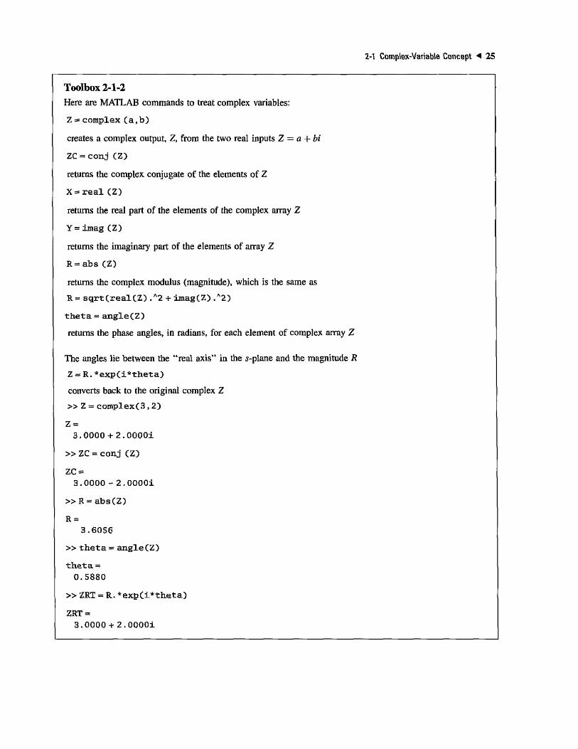
Toolbox 2-1-2
Here are MATLAB commands to treat complex variables:
Z = complex ( a , b )
creates a complex output, Z, from the two real inputs Z — a-\- bi
ZC = con j (Z)
returns the complex conjugate of the elements of Z
X = r e a l (Z)
returns the real part of the elements of the complex array Z
Y=imag (Z)
returns the imaginary part of the elements of array Z
R= abs (Z)
returns the complex modulus (magnitude), which is the same as
R= s q r t ( r e a l ( Z ) .A2 + imag(Z) .A2)
t h e t a = a n g l e ( Z )
returns the phase angles, in radians, for each element of complex array Z
The angles lie between the "real axis" in the s-plane and the magnitude R
Z = R . * e x p ( i * t h e t a )
converts back to the original complex Z
» Z = complex (3 ,2 )
Z = 3.0000 + 2 .00001
» ZC = conj (Z)
ZC = 3.0000 - 2.0000i
» R = abs(Z)
R = 3.6056
» theta= angle(Z)
theta = 0.5880
» ZRT = R.*exp(i*theta)
ZRT = 3.0000 + 2.00001

26 Chapter 2. Mathematical Foundation
where (-/^) and (-p2) are poles of the function G(s). By definition, if s = jco, G( jco) is the frequency response function of G(s), because co has a unit of frequency (rad/s):
G(s) = ——- * - (2-35)
The magnitude of G( y<y) is
R = |C( » | = — £ — (2-36)
and the phase angle of G( jco) is
¢=/-0( jco) = / K — / /Vo 4- /?i — / JKU + P2
= -01 - 02
For the general case, where
(2-37)
C(.v) = K - ^ (2-38)
J>+Pf) c=i
The magnitude and phase of G{s) are as follows
» \r>< > M «» lj«» + Zl1-**l/» + a« 7<»+Pi[---1/0)+PIII (2-39)
0 = / G ( » = (f i + • • • + fm) - ( 0 , + - - -+ 0„)
2-2 FREQUENCY-DOMAIN PLOTS
Let G(s) be the forward-path transfer function1 of a linear control system with unity feedback. The frequency-domain analysis of the closed-loop system can be conducted from the frequency-domain plots of G(s) with s replaced by jco.
The function G( jco) is generally a complex function of the frequency co and can be written as
G(j(o) = \G(jco)\lG(jco) (2-40)
where |G(,/w)| denotes the magnitude of G(jco), and /G(jco) is the phase of G(jco). The following frequency-domain plots of G(jco) versus co are often used in the
analysis and design of linear control systems in the frequency domain.
1. Polar plot. A plot of the magnitude versus phase in the polar coordinates as co is varied from zero to infinity
2. Bode plot. A plot of the magnitude in decibels versus co (or log|0a>) in semilog (or rectangular) coordinates
3. Magnitude-phase plot. A plot of the magnitude (in decibels) versus the phase on rectangular coordinates, with co as a variable parameter on the curve
2-2-1 Computer-Aided Construction of the Frequency-Domain Plots
The data for the plotting of the frequency-domain plots are usually quite time consuming to generate if the computation is carried out manually, especially if the function is of high order. In this textbook, we use MATLAB and the ACSYS software for this purpose.
For the formal definition of a "transfer function,*' refer to Section 2-7-2.

2-2 Frequency-Domain Plots 27
JO)
2 Polar Plots
.v-planc
--joh
JCOf
j Im C
G(j(0)-p\ane
ReG
Figure 2-8 Polar plot shown as a mapping of the positive half of the yVt»-axis in the s-plane onto the G( y«)-plane.
From an analytical standpoint, the analyst and designer should be familiar with the properties of the frequency-domain plots so that proper interpretations can be made on these computer-generated plots.
The polar plot of a function of the complex variable s, G(s), is a plot of the magnitude of G( jco) versus the phase of G( jco) on polar coordinates as co is varied from zero to infinity. From a mathematical viewpoint, the process can be regarded as the mapping of the positive half of the imaginary axis of the s-plane onto the G( /<y)-plane. A simple example of this mapping is shown in Fig. 2-8. For any frequency co — co\, the magnitude and phase of G(jco]) are represented by a vector in the G(jco)-plane. In measuring the phase, counterclockwise is referred to as positive, and clockwise is negative.
EXAMPLE 2-2-1 To illustrate the construction of the polar plot of a function G(s), consider the function
1 G(s) =
1+Ts
where T is a positive constant. Setting s = jco, we have
1 G(jco) =
1 + jcoT
In terms of magnitude and phase, Eq. (2-42) is rewritten as
1 G{jco) =
V\ + co2T2
(2-41)
(2-42)
(2-43)
When co is zero, the magnitude of G(jco) is unity, and the phase of G(jco) is at 0°. Thus, at co — 0, G(jco) is represented by a vector of unit length directed in the 0° direction. As co increases, the magnitude of G( jco) decreases, and the phase becomes more negative. As co increases, the length of the vector in the polar coordinates decreases and the vector rotates in the clockwise (negative) direction. When co approaches infinity, the magnitude of G( jco) becomes zero, and the phase reaches -90° . This is presented by a vector with an infinitesimally small length directed along the -90°-axis in the G(jco)-plane. By substituting other finite values of co into Eq. (2-43), the exact plot of G(jco) turns out to be a semicircle, as shown in Fig. 2-9.

28 Chapter 2. Mathematical Foundation
jlmG G (/'ft>)-plane
Figure 2-9 Polar plot of G( jco) = l
\+jo>TY
EXAMPLE 2-2-2 As a second illustrative example, consider the function
where T\ and T2 are positive real constants. Eq. (2-44) is re-written as
,>2T2
1 + CO I i
(2-44)
(2-45)
The polar plot of G( ycu), in this case, depends on the relative magnitudes of T\ and T2. If T2 is greater than T\, the magnitude of G( y'o)) is always greater than unity as co is varied from zero to infinity, and the phase of G( jco) is always positive. If T2 is less than 2*1, the magnitude of G( jco) is always less than unity, and the phase is always negative. The polar plots of G(jco) of Eq. (2-45) that correspond to these two conditions are shown in Fig. 2-10.
The general shape of the polar plot of a function G( jco) can be determined from the following information.
1. The behavior of the magnitude and phase of G( jco) at co = 0 and co — co.
2. The intersections of the polar plot with the real and imaginary axes, and the values of co at these intersections
j Im G
(T2 < 7",)
Figure 2-10 Polar plots of G( jco) = (1 + Ja>T2) {l+jo>Ti)'
TJT, Re G

2-2 Frequency-Domain Plots 29
Toolbox 2-2-1
The Nyquist diagram for Eq. (2-44) for two cases is obtained by the following sequence of MATLAB functions:
Tl = 10; T2 = 5; nural = [T2 1] ; denl = [Tl 1] ; Gl=tf(numl,denl); nyquist(Gl); hold on; num2 = [Tl 1] ; den2 = [T2 1] ; G2 = tf (num2,den2) ; nyquist (G2) ; title ( ' Nyquist diagram of Gl and G2' )
Note: The "nyquist" function provides a complete polar diagram, where co is varying from — oo to -t-oc.
Nyquist diagram of G1 and G2 0.5 p
0.4 -
0.3 -
0.2 -
w 0.1 -
g «3
E -0.1 -
-0,2 -
-0.3 -
-0.4 -
-0.5 -
-1 -0.5 0 0.5 1 1.5 2
Comparing the results in Toolbox 2-2-1 and Fig. 2-10, it is clear that the polar plot reflects only a portion of the Nyquist diagram. In many control-system applications, such as the Nyquist stability criterion (see Chapter 8), an exact plot of the frequency response is not essential. Often, a rough sketch of the polar plot of the transfer function is adequate for stability analysis in the frequency domain.

30 Chapter 2. Mathematical Foundation
EXAMPLE 2-2-3 In frequency-domain analyses ofcontrol systems, often we have to determine the basic properties of a polar plot. Consider the following transfer function:
°W=^TT) ( 2- 4 6> By substituting s = jco in Eq. (2-46), the magnitude and phase of G( jco) at co = 0 and co = oo are computed as follows:
lim |O(/0>)| = lim — = oo <u—»0 <u—»0 Co
lim /G{jco) = lim l\0/jco = -90° o) —»0 co —»0
lim \G(jco)\= lim - ^ = 0 a) —• oo o) —> oc ( y -
lim /.G{jco) = lim /lO/ycy2 = - 1 8 0 °
(2-47)
(2-48)
(2-49)
(2-50)
Thus, the properties of the polar plot of G( jco) atco = 0 and w = oc are ascertained. Next, we determine the intersections, if any, of the polar plot with the two axes of the G( jco)-p\ane. If the polar plot of G( jco) intersects the real axis, at the point of intersection, the imaginary part of G(jco) is zero; that is,
lm[G(jco)] = 0 (2-51)
To express G(jco) as the sum of its real and imaginary parts, we must rationalize G(jco) by multiplying its numerator and denominator by the complex conjugate of its denominator. Therefore, G(jco) is written
\0{-jco){-jco+\) - 1 0 f t ) 2 10tt> ~ V + o>2 (2-52) G(jco) = -J jco{ jco +l){-jco){-jco+l) co4
= Rc[G(jco)] + jlm[G(jco)]
When we set Im[G( jco)] to zero, we get co = oo, meaning that the G( jco) plot intersects only with the real axis of the G(jco)-plane at the origin.
Similarly, the intersection of G(jco) with the imaginary axis is found by setting Re[G(ya>)] of Eq. (2-52) to zero. The only real solution for co is also co ~ oo, which corresponds to the origin of the G( jco)-p\ane. The conclusion is that the polar plot of G( jco) does not intersect any one of the axes at any finite nonzero frequency. Under certain conditions, we are interested in the properties of the G( jco) at infinity, which corresponds to co = 0 in this case. From Eq. (2-52), we see that lm[G( jco)] = oo and Re[G( jco)] = —10 at co = 0. Based on this information as well as knowledge of the angles of G(jco) at co = 0 and co = oo, the polar plot of G(jco) is easily sketched without actual plotting, as shown in Fig. 2-11.
G(/'(U)-plano jlmG'
— 10 Figure 2-11 Polar plot of G{s) = -^+rr

2-2 Frequency-Domain Plots < 31
EXAMPLE 2-2-4 Given the transfer function
G(s) = 10
(2-53) s(s+\)(s + 2)
we want to make a rough sketch of the polar plot of G( jco). The following calculations are made for the properties of the magnitude and phase of G(jco) at (o = 0 and co = oo:
lim \G{ /ft)) I — lim — = oo co — 0 co —Oft)
lim /.G(jo))= lim /5/jco ~-90c
co—»0 <w — 0
10
(2-54)
(2-55)
lim \G(ja>)\= lim -^ = 0 (2-56) CO —» OC CO —» CO ft)-1
To find the intersections of the G(jco) plot on the real and imaginary axes of the G(jco)-plane, we rationalize G(jco) to give
\0{-jco)(-jco + ! ) ( - > + 2) ^ Xyft ) + l)(/ft) + 2 ) ( - » ( - y f t ) + l)(-yVu + 2)
After simplification, the last equation is written
G(j(o) = Re[G(y'ft))] 4- jlm[G(jco)} = -30 710(2 - •2\
(2-57)
(2-58) 9ft)2 + ( 2 - a)2)2 9ft)3 -I- 0)(2 - ft)2)2
Setting Re[G(y"ft))] to zero, we have co = oc, and G(y'oo) = 0, which means that the G(jco) plot intersects the imaginary axis only at the origin. Setting Im[G( jco)} to zero, we have co = ±\/2 rad/sec. This gives the point of intersection on the real axis at
G(±yV2) = - 5 / 3 (2-59)
The result, co = —y/2 rad/sec, has no physical meaning, because the frequency is negative; it simply represents a mapping point on the negative y'ft)-axis of the j-plane. In general, if G(s) is a rational function of .v (a quotient of two polynomials of „?), the polar plot of G( jco) for negative values of co is the mirror image of that for positive co, with the mirror placed on the real axis of the G(y'ft>)-plane. From Eq. (2-58), we also see that Re[G(y'0)] = oc and lm[G(y'0)] = oo. With this information, it is now possible to make a sketch of the polar plot for the transfer function in Eq. (2-53), as shown in Fig. 2-12.
Although the method of obtaining the rough sketch of the polar plot of a transfer function as described is quite straightforward, in general, for complicated transfer functions that may have multiple crossings on the real and imaginary axes of the transfer-function plane, the algebraic manipulation may again be quite involved. Furthermore, the polar plot is basically a tool for analysis; it is somewhat awkward for design purposes. We shall show in the next section that approximate information on the polar plot can always be obtained from the Bode plot, which can be sketched
G-plane
Figure 2-12 Polar plot of G(s) = 10 sts+lM-H-2)"

Chapter 2. Mathematical Foundation
without any calculations. Thus, for more complicated transfer functions, sketches of the polar plots can be obtained with the help of the Bode plots, unless MATLAB is used.
Bode Plot (Corner Plot or Asymptotic Plot)
The Bode plot of the function G( jco) is composed of two plots, one with the amplitude of G(jco) in decibels (dB) versus log10a) or co and the other with the phase of G{jco) in degrees as a function of log10o) or co. A Bode plot is also known as a corner plot or an asymptotic plot of G(jco). These names stem from the fact that the Bode plot can be constructed by using straight-line approximations that are asymptotic to the actual plot.
In simple terms, the Bode plot has the following features:
1. Because the magnitude of G( jco) in the Bode plot is expressed in dB, product and division factors in G[ jco) became additions and subtractions, respectively. The phase relations are also added and subtracted from each other algebraically.
2. The magnitude plot of the Bode plot of G( jco) can be approximated by straight-line segments, which allow the simple sketching of the plot without detailed computation.
Because the straight-line approximation of the Bode plot is relatively easy to construct, the data necessary for the other frequency-domain plots, such as the polar plot and the magnitude-versus-phase plot, can be easily generated from the Bode plot.
Consider the function
c(s) = y+^+^)-(; + ̂ )g-^ (2.60) W sJ(s+Pi){s+P2)---{s+P»)
where K and T(/ are real constants, and the z's and the ;;'s may be real or complex (in conjugate pairs) numbers. In Chapter 7, Eq. (2-60) is the preferred form for root-locus construction, because the poles and zeros of G(.v) are easily identified. For constructing the Bode plot manually, G(s) is preferably written in the following form:
/ : ,0+ ^ ) d + ^) - - - (1+ rw.v) TdS U{S) */{l + Ta.s)(l + Ths) - - - ( 1 + T„s) U ° U
where K\ is a real constant, the Fs may be real or complex (in conjugate pairs) numbers, and Trfis the real time delay. If the Bode plot is to be constructed with a computer program, then either form of Eq. (2-60) or Eq. (2-61) can be used.
Because practically all the terms in Eq. (2-61) are of the same form, then without loss of generality, we can use the following transfer function to illustrate the construction of the Bode diagram.
C ( v ) = ^ 1 + ^ ) ( 1 + ^ ) e-Tl, ( 9 „ 6 2 )
°[S) s( 1 + TaS) (1 + 2fsM, + j*/«Q (- *Z)
where K, Tc/, T\, T2, Ta, f, and con are real constants. It is assumed that the second-order polynomial in the denominator has complex-conjugate zeros.
The magnitude of G( jco) in dB is obtained by multiplying the logarithm (base 10) of \G(jco)\ by 20; we have
| G ( » | d B = 2 0 1 o g H ) | G ( . H |
= 20logi0|AT| + 201og10| 1 + jcoTi | + 20 log1()| 1 4- jcoT2\
- 2 0 1 o g 1 0 | > | -201og1 0 | l +j<oTa\ -201og1 0 | l + j2t;co- co2/col\ (2-63)

2-2 Frequency-Domain Plots 33
The phase of G( jco) is
/_G{ jco) = IK + /(1 + jtoT\ ) + / ( 1 + M 2 ) - I jco - / ( 1 + > r f l
- / ( 1 + 2$to/con - a)2 /&>*) — )̂7 /̂ rad (2-64)
In general, the function G(jco) may be of higher order than that of Eq. (2-62) and have many more factored terms. However, Eqs. (2-63) and (2-64) indicate that additional terms in G(jco) would simply produce more similar terms in the magnitude and phase expressions, so the basic method of construction of the Bode plot would be
Toolbox 2-2-2
The Bode plot for Example 2-1-3, using the MATLAB "bode" function, is obtained by the following sequence of MATLAB functions.
Approach 1
num = [ 1 6 ] ; d e n = [1 10 16] ; G = t f ( n u m , d e n ) ; bode(G) ;
Approach 2
s - t f C s * ) ; G=16/(sA2 + 10*s + 1 6 ) ; bode(G) ;
The "bode" function computes the magnitude and phase of the frequency response of linear time invariant models. The magnitude is plotted in decibels (dB) and the phase in degrees. Compare the results to the values in Table 2-2.
Bode Diagram - T 1 1 1—I I I I J
- 2 0 -
m >—* ID ' ' •
-•
CI on ^
/—-. IM m
• r , • - — • •
« 03
-40
-60
-80
-100 0
-45
-90
- I 1 1 — I — I I I I I
_l 1—I I I I - - L I I I I I I I - I i 1—L_J_
-135
-180 =
~T 1 1—i—r
10

34 t> Chapter 2. Mathematical Foundation
the same. We have also indicated that, in general, G(jco) can contain just five simple types of factors:
1. Constant factor: K
2. Poles or zeros at the origin of order/;: (jco) p
3. Poles or zeros at s — — l/T of order q: (1 + jcoT) q
4. Complex poles and zeros of order r: (l + j2$co/con — ar/co^)
5. Pure time delay e"J d, where T(/, p, q, and r are positive integers
Eqs. (2-63) and (2 64) verify one of the unique characteristics of the Bode plot in that each of the five types of factors listed can be considered as a separate plot; the individual plots are then added or subtracted accordingly to yield the total magnitude in dB and the phase plot of G(jco). The curves can be plotted on semilog graph paper or linear rectangular-coordinate graph paper, depending on whether co or log10ft> is used as the abscissa.
We shall now investigate sketching the Bode plot of different types of factors.
2-2-4 Real Constant K
Because
KdB = 2 0 log 1 0 # = constant (2-65)
and
.„ /o° A:>O _ Z * = \ 1 8 0 ° K<0 ( 2 " 6 6 )
the Bode plot of the real constant K is shown in Fig. 2-13 in semilog coordinates.
2-2-5 Poles and Zeros at the Origin, (jco)±p
The magnitude of {jco)±p in dB is given by
201og10 jco)±p = ±20plog10w dB (2-67)
for co > 0. The last expression for a given p represents a straight line in either semilog or rectangular coordinates. The slopes of these lines are determined by taking the derivative of Eq. (2-67) with respect to log)0ft;; that is,
(±20 p log l0eo) = ± 2 0 p dB/decade (2-68) d\ogl0co
These lines pass through the 0-dB axis at co = 1. Thus, a unit change in log10w corresponds to a change of ±20p dB in magnitude. Furthermore, a unit change in log^co in the rectangular coordinates is equivalent to one decade of variation in co, that is, from 1 to 10, 10 to 100, and so on, in the semilog coordinates. Thus, the slopes of the straight lines described by Eq. (2-68) are said to be ±20 p dB/decade of frequency.

2-2 Frequency-Domain Plots 35
a'
40
30
20
10
0
-10
-20
-30
1̂0
| 20 log
V l0KdB(K= 10)
0.1 co (rad/sec)
10 100
a O
90
60
30
-30
-60
-90
-120
-150
-180
SLK
lL
/
(K>
K(K
0)
<0)
0.1
Figure 2-13 Bode plot of constant K.
co (rad/sec) 10 100
Instead of decades, sometimes octaves are used to represent the separation of two frequencies. The frequencies co\ and C02 are separated by one octave if 0)2/'co\ = 2. The number of decades between any two frequencies cx>\ and u>2 is given by
number of decades = — - ^ —— = login ( — log1010 IUV«i
Similarly, the number of octaves between a>2 and co\ is
log 10 (^2/^1) number of octaves —
logio2
Thus, the relation between octaves and decades is
okI o g l 0&
(2-69)
(2-70)
number of octaves = 1/0.301 decades = 3.32 decades (2-71)

Mathematical Foundation
Substituting Eq. (2-71) into Eq. (2-67), we have
±20;?dB/decade = ±20 p x 0.301 ar 6/? dB/octave (2-72)
For the function G(s) — 1 /s, which has a simple pole at s — 0, the magnitude of G( jco) is a straight line with a slope of —20dB/decade, and it passes through the 0-dB axis at co = 1 rad/sec.
The phase of (jco) p is written
\±P-l(j(orp=±p x90c (2-73)
The magnitude and phase curves of the function (jco) p are shown in Fig. 2-14 for several values of P.
60
40
20
0
a c -20
-40
-60
\
1̂
^
, , ^ J C ^ *
' % > *GJ
P\
\
%
+7.0
30
^
UeJfi
2S**,
0))
#y j
0.1
180
90
a -90
-180
-270
co (rad/sec)
10
100
/ S-{j(QT
MVjco)
^(1/yfi))2
-6(/6)) , ^
100 co (rad/sec)
Figure 2-14 Bode plots of (to)^,
2-2 Frequency-Domain Plots 37
2-2-6 Simple Zero, 1 +ja>T
Consider the function
G(jco) = l + jcoT (2-74)
where T is a positive real constant. The magnitude of G(jco) in dB is
\G(jco)\dB = 2 0 ! o g 1 0 | G ( » l = 201og10\/l + co2T2 (2-75)
To obtain asymptotic approximations of \G(jco)\dB, we consider both very large and very small values of co. At very low frequencies, coT-C 1. Eq. (2-75) is approximated by
| C ( » | d B ^ 2 0 1 o g 1 0 l = 0 dB (2-76)
because co2T2 is neglected when compared with I. At very high frequencies, coT^> 1, we can approximate 1 + co2T2 by co~T2; then Eq.
(2-75) becomes
| G ' ( » | d B = 201og] 0V^T2 = 201og10a>r (2-77)
Eq. (2-76) represents a straight line with a slope of 20 dB/decade of frequency. The intersect of these two lines is found by equating Eq. (2-76) to Eq. (2-77), which gives
to = l/T (2-78)
This frequency is also the intersect of the high-frequency approximate plot and the low-frequency approximate plot, which is the 0-dB axis. The frequency given in Eq. (2-78) is also known as the corner frequency of the Bode plot of Eq. (2-74), because the asymptotic plot forms the shape of a corner at this frequency, as shown in Fig. 2-15. The actual \G( jco) |dB plot of Eq. (2-74) is a smooth curve and deviates only slightly from the straight-line approximation. The actual values and the straight-line approximation of j 1 + jcoT\6B
as functions of coT are tabulated in Table 2-3. The error between the actual magnitude curve and the straight-line asymptotes is symmetrical with respect to the corner frequency co = l/T. It is useful to remember that the error is 3 dB at the corner frequency, and it is 1 dB at 1 octave above (co = 2/T) and 1 octave below (co — 1/27") the corner frequency. At 1 decade above and below the corner frequency, the error is dropped to approximately 0.3 dB. Based on these facts, the procedure of drawing |1 + jcoT\dB is as follows:
1. Locate the corner frequency co = l/T on the frequency axis.
2. Draw the 20-dB/decade (or 6-dB/octave) line and the horizontal line at 0 dB, with the two lines intersecting at co = l /T.
3. If necessary, the actual magnitude curve is obtained by adding the errors to the asymptotic plot at the strategic frequencies. Usually, a smooth curve can be sketched simply by locating the 3-dB point at the corner frequency and the 1-dB points at 1 octave above and below the corner frequency.
The phase of G(jco) = 1 + jcoT is
/G( jco) = tan"' coT (2-79)
Similar to the magnitude curve, a straight-line approximation can be made for the phase curve. Because the phase of G( jco) varies from 0° to 90°, we can draw a line from 0° at 1 decade below the corner frequency to 90° at 1 decade above the corner frequency. As shown in Fig. 2-15, the maximum deviation between the straight-line approximation and the actual curve is less than 6°. Table 2-3 gives the values of /(1 + jcoT) versus coT.

38 Chapter 2. Mathematical Foundation
2 a
40
20
-20
-40
f ^ / l\
/"
G(s) = 1 + symptotes
1 1
i 5W = M
" • ^ ^
Ts
Ts
0.01 0.1 1 (oT
10 100
3 a
90
60
30
-30
-60
-90
G(s) = ] 1
+ 7 /
s /
< 3(s) = 1 + Ts
0.01 0.1 1 10 100
Figure 2-15 Bode plots of G(s) = 1 + Ts and G(s) = TJ +TsY
TABLE 2-3 Values of ./(1 + /wfjversus wT
Straight-Line
6)T
0.01
0.10
0.50
0.76
1.00
1.31
2.00
10.00
100.00
iog|0wr
- 2
- 1
-0 .3
-0.12
0
0.117
0.3
1.0
2.0
\l + ja>T\
1.0
1.04
1.12
1.26
1.41
1.65
2.23
10.4
100.005
Approximation
\l+Ja>T\dB
0.000043
0.043
1
2
3
4.3
7.0
20.043
40.00043
1.1 +JQ>T\aB
0
0
0
0
0
2.3
6.0
20.0
40.0
Error 1(1
(dB)
0.00043
0.043
1
2
3
2
1
0.043
0.00043
+ JuT)
(deg)
0.5
5.7
26.6
37.4
45.0
52.7
63.4
84.3
89.4

2-2 Frequency-Domain Plots 39
2-2-7 Simple Pole, 1/(1 +jcoT)
For the function
G(jco) = 1
1 + jeoT (2-80)
the magnitude, \G( jco) | in dB, is given by the negative of the right side of Eq. (2-75), and the phase IG{ jco) is the negative of the angle in Eq. (2-79). Therefore, it is simple to extend all the analysis for the case of the simple zero to the Bode plot of Eq. (2-80). The asymptotic approximations of \G( jco)]^ at low and high frequencies are
w r < l iGO&OldB ^ O d B
coT^l | G ( » | d B S -20log10o)T
(2-81)
(2-82)
Thus, the corner frequency of the Bode plot of Eq. (2-80) is still at to = 1/7, except that at high frequencies the slope of the straight-line approximation is -20dB/decade. The phase of G( jco) is 0 degrees at co = 0, and —90° when co — oo. The magnitude in dB and phase of the Bode plot of Eq. (2-80) are shown in Fig. 2-15. The data in Table 2-3 are still useful for the simple-pole case if appropriate sign changes are made to the numbers. For instance, the numbers in |1 + jcoT\dB, the straight-line approximation of |1 + jcoT\dB, the error (dB), and the /(1 + jcoT) columns should all be negative. At the corner frequency, the error between the straight-line approximation and the actual magnitude curve is — 3 dB.
2-2-8 Quadratic Poles and Zeros
Now consider the second-order transfer function
G(s) = cot s2 + 2$a)„s + co2 1 + (2;/con)s + (l/co2
n)s2 (2-83)
We are interested only in the case when £ < 1, because otherwise G(s) would have two unequal real poles, and the Bode plot can be obtained by considering G(s) as the product of two transfer functions with simple poles.
By letting s — jco, Eq. (2-83) becomes
G ( » = T
1
1 - (Co/On) + J2$(c0/C0n)
The magnitude of G( jco) in dB is
? 1 2
(2-84)
\G(jco)\ = 2 0 1 o g I 0 | G ( » | = -201og 1 0 y | l - (co/cvn)z\ +4?(co/con)
2 (2-85)
At very low frequencies, co/con >C 1, Eq. (2-85) can be approximated as
| G ( » l d B = 2 0 1 o g 1 0 | G ( » | £ - 201og10l = 0 dB (2-86)
40 Chapter 2. Mathematical Foundation
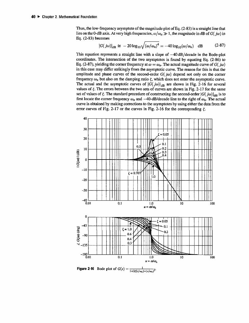
Thus, the low-frequency asymptote of the magnitude plot of Eq. (2-83) is a straight line that lies on the 0-dB axis. At very high frequencies, co/con » 1, the magnitude in dB of G( jco) in Eq. (2-83) becomes
dB (2-87) \G(ja>)\dB £ -2Q\ogX0y/(Q>/conf = -40\og}0{co/a)n
This equation represents a straight line with a slope of -40dB/decade in the Bode-plot coordinates. The intersection of the two asymptotes is found by equating Eq. (2-86) to Eq. (2-87), yielding the corner frequency at co — eon. The actual magnitude curve of G( jco) in this case may differ strikingly from the asymptotic curve. The reason for this is that the amplitude and phase curves of the second-order C( jco) depend not only on the corner frequency co„ but also on the damping ratio £, which does not enter the asymptotic curve. The actual and the asymptotic curves of |C(v'w)ldB are shown in Fig. 2-16 for several values of £. The errors between the two sets of curves are shown in Fig. 2-17 for the same set of values of f. The standard procedure of constructing the second-order | G( jco) |dB is to first locate the corner frequency con and —40-dB/decade line to the right of co„. The actual curve is obtained by making corrections to the asymptotes by using either the data from the error curves of Fig. 2-17 or the curves in Fig. 2-16 for the corresponding £.
40
30
20
10
"S 0 ^> o
-10
-20
-30
-40 0.
1 =
0.5
0.7
\
07
/ /
\.y
1.0
£ = <
^ 1 , r
).0.
.1
.2
.3
.4
\
\ 1 \
01 0.1 1.0 It = 0)10),,
10 100
,-. -45 oo 0)
§ -90
s ^ -135
-180
1= ( (
y 1.0
).6 ' ).4 ' ).3-
/ /
y
3ty— £
JS
= 0 05
0.1
0.2
0.01 0.1 1.0 U - 0)1(1),,
10 100
Figure 2-16 Bode plot of G{s) = I+2f(jr /^ )+(*/«>»)-

2-2 Frequency-Domain Plots < 41
'a O
25
20
15
10
-5
-10
-15
II
' V ^ £=0.05 i i I 1
f U 1 1 7 \ \ 0.2'
7 YvC^°'3
^fp^^O.4 "
. JK r o.6 " T 0.707
1.0
0.01 0.1 1.0 10
Figure 2-17 Errors in magnitude curves of Bode plots of G(s) =
100
+2f(*/»„ )+(*/»„)-'
The phase of G( ja>) is given by
/G{jco) = -tan - i | 2 < ^
<% 1 - — (2-88)
and is plotted as shown in Fig. 2-16 for various values of £". The analysis of the Bode plot of the second-order transfer function of Eq. (2-83) can be
applied to the second-order transfer function with two complex zeros. For
G(s)= 1+ — s + 1
a: (2-89)
the magnitude and phase curves are obtained by inverting those in Fig. 2-16. The errors between the actual and the asymptotic curves in Fig. 2-17 are also inverted.
Toolbox 2-2-3
The Bode plot for Fig. 2-17 when £ = 0.05 and co—l, using the MATLAB "bode" function, is obtained by the following sequence of MATLAB functions.
Approach 1
num = [ 1 ] ; d e n = [ 1 . 1 1 ] ; G = t f ( n u m , d e n ) ; bode(G) ;
Approach 2
s = t f ( ' s ' ) ; G = l / ( s A 2 + .1*3 + 1 ) ; bodeCG);

42 Chapter 2. Mathematical Foundation
40 r
20
! -20 -
/—s Cfl ID
T3.
<D
CQ J = Q-
-40 0
-45
-90 -
-135
-180 =-
io-1
Bode Diagram i—i i i i -i 1 1 1—i—i—r
_i i i i L _i i i i l u
10 Frequency (rad/sec)
2-2-9 Pure Time Delay, e~/toTrf
The magnitude of the pure time delay term is equal to unity for all values of co. The phase of the pure time delay term is
le-jcoT, _ _cojd ( 2 _ 9 0 )
which decreases linearly as a function of co. Thus, for the transfer function
G{jco) = Gx{jco)e-JcoT" (2-91)
the magnitude plot \G{ jco) | d B is identical to that of \G\ (jco)|dB. The phase plot IG( jco) is obtained by subtracting coTj radians from the phase curve of G\ (jco) at various co.
EXAMPLE 2-2-5 As an illustrative example on the manual construction of the Bode plot, consider the function
10(5+ 10) G{s) = (2-92)
s{s + 2)(.9 + 5)
The first step is to express G(s) in the form of Eq. (2-61) and set.? = jco (keeping in mind that, for computer plotting, this step is unnecessary); we have
10(1 + j0.\co) G(jco) =
jco(\ + j0.5co)(l + j0.2co) (2-93)
Eq. (2-92) shows that G(jco) has corner frequencies at co = 2, 5, and 10 rad/sec. The pole at s = 0 gives a magnitude curve that is a straight line with a slope of —20 dB/decade, passing through the co = 1 rad/sec point on the 0-dB axis. The complete Bode plot of the magnitude and phase of G( jco) is obtained by adding the component curves together, point by point, as shown in Fig. 2-18. The actual curves can be obtained by a computer program and are shown in Fig. 2-18.

2-2 Frequency-Domain Plots 43
40
20
-20
a O -40
-60
-80
-100
^ -20 dB/sec
Gain crossover 3.88 rad/sec
-40 dB/sec
\ i k - - - 6 0 dB/sec
^S X s *r 40 dB/se
0.10
-90
-120
-150
S £> -180 O
-210
-240
-270
5 10 <y (rad/sec)
100 1000
Phase crossover , 5.78 rad/sec
/
0.10
Figure 2-18 Bode plot of G(s) =
2 5 10 ft) (rad/sec)
10(5+10)
100 1000
5(j+2)(s+5)-
Toolbox 2-2-4
The Bode plot for Eq. (2-93), using the MATLAB "bode" function, is obtained by the following sequence of MATLAB functions.
num= [ 1 10] ; den = [ . 1 . 7 1 0 ] ; G = t f ( n u m . d e n ) ; bode(G) ;
The result is a graph similar to Fig. 2-18.

44 Chapter 2. Mathematical Foundation
2-2-10 Magnitude-Phase Plot
The magnitude-phase plot of G( jco) is a plot of the magnitude of G( jco) in dB versus its phase in degrees, with w as a parameter on the curve. One of the most important applications of this type of plot is that, when G( jco) is the forward-path transfer function of a unity-feedback control system, the plot can be superposed on the Nichols chart (see Chapter 8) to give information on the relative stability and frequency response of the system. When constant coefficient K of the transfer function varies, the plot is simply raised or lowered vertically according to the value of K in dB. However, in the construction of the plot, the property of adding the curves of the individual components of the transfer function in the Bode plot does not carry over to this case. Thus, it is best to make the magnitude-phase plot by computer or transfer the data from the Bode plot.
EXAMPLE 2-2-6 As an illustrative example, the polar plot and the magnitude-phase plot of Eq. (2-92) are shown in Fig. 2-19 and Fig. 2-20, respectively. The Bode plot of the function is already shown in Fig. 2-18. The relationships among these three plots are easily identified by comparing the curves in Figs. 2-18, 2-19, and 2-20.
jlmG
G-plane
Figure 2-19 Polar plot of G(s) = J V S , 0 ) ,v(.v+2)(.v+5)

2-2 Frequency-Domain Plots 45
40
30
20
10
0
-10 CO - a
1 -20
-30
^10
-50
-60
-70
-80
Phase crossover 0) = 5.78 rad/sec""""""---̂
i
0) = 10 ra
co = 30 n
« = 1 0 0
d/sec-
fifKPC ...
/
U/ o t t — l — n
rad/sec
3 1 8
" Gain cr G)=3.8i
yT(0 =
ossover \ rad/sec
V
1 rad/sec
-270.0 -247.5 -225.0 -202.5 -180.0 -157.5 -135.0 -112.5 -90.0
Phase(deg)
Figure 2-20 Magnitude-phase plot of G(s) = ^ ° ¾ ¾ •
Toolbox 2-2-5
The magnitude and phase plot for Example 2-2-6 may be obtained using the MATLAB "nichols" function, by the following sequence of MATLAB functions.
» G = z p k ( [ - 1 0 ] , [0 -2 - 5 ] ,10)
Zero/pole/gain:
10 (s + 10
s Cs + 2) (s + 5)
» nichols(G)
See Fig. 2-20.

46 Chapter 2. Mathematical Foundation
Toolbox 2-2-6
The phase and gain margins for Eq. (2-92) are obtained by the following sequence of MATLAB functions.
Approach 1
num = [10 100] ; d e n = [1 7 10 0 ] ; Gl = t f ( n u m , d e n ) ; marginCGI) ;
Approach 2
s = t f ( ' s ' ) ; Gl=(10-s + 1 0 0 ) / ( s A 3 + 7"sA2 + I0*s) ; m a r g i n ( G l ) ;
"Margin" produces a Bode plot and displays the margins on this plot.
60
40
in i ••
w 11 L5
±=t c rr. in
?o
0
-20
-40
-60 -90
3 -135 0)
03
if -180
-225 --
Bode Diagram Gm = 7.36 dB (at 5.77 rad/sec), Pm * 10.7 deg (at 3.88 rad/sec)
i ' i i i i L_LJ i • '• • '• i i i I i i i i i t i > -
| - ~ 1 1 ' 1 1—I—r-r-j 1 1 n 1—n—i—i i | 1 1 1 1 1—i—i i—i
= 1 i I I I 1 ' ' I I I i I I ' ' • I I I I I f I... ' i -
2-2-11 Gain- and Phase-Crossover Points
Gain- and phase-crossover points on the frequency-domain plots are important for analysis and design of control systems. These are defined as follows.
• Gain-crossover point. The gain-crossover point on the frequency-domain plot of G(jco) is the point at which |G(y'a>)| = 1 or \G(j(o)\dB = 0 dB. The frequency at the gain-crossover point is called the gain-crossover frequency cog.
• Phase-crossover point. The phase-crossover point on the frequency-domain plot of G(jco) is the point at which IG(jio) = 180°. The frequency at the phase-crossover point is called the phase-crossover frequency cop.

2-2 Frequency-Domain Plots 47
The gain and phase crossovers are interpreted with respect to three types of plots:
• Polar plot. The gain-crossover point (or points) is where \G(jco) | = I. The phase-crossover point (or points) is where /.G(jco) = 180° (see Fig. 2-19).
• Bode plot. The gain-crossover point (or points) is where the magnitude curve \G( jco) |()B crosses the 0-dB axis. The phase-crossover point (or points) is where the phase curve crosses the 180° axis (see Fig. 2-18).
• Magnitude-phase plot. The gain-crossover point (or points) is where the G( jco) curve crosses the 0-dB axis. The phase-crossover point (or points) is where the G(jco) curve crosses the 180° axis (see Fig. 2-20).
2-2-12 Minimum-Phase and Nonminimum-Phase Functions
A majority of the process transfer functions encountered in linear control systems do not have poles or zeros in the right-half .9-plane. This class of transfer functions is called the minimum-phase transfer function. When a transfer function has either a pole or a zero in the right-half .9-plane, it is called a nonminimum-phase transfer function.
Minimum-phase transfer functions have an important property in that their magnitude and phase characteristics are uniquely related. In other words, given a minimum-phase function G(.9), knowing its magnitude characteristics |G(jw)| completely defines the phase characteristics, IG(jco). Conversely, given IG(jco), \G(jco)\ is completely defined.
Nonminimum-phase transfer functions do not have the unique magnitude-phase relationships. For instance, given the function
G<»=T^r (2"94>
the magnitude of G( jco) is the same whether T is positive (nonminimum phase) or negative (minimum phase). However, the phase of G( jco) is different for positive and negative T.
Additional properties of the minimum-phase transfer functions are as follows:
• For a minimum-phase transfer function G(s) with in zeros and n poles, excluding the poles at .9 = 0, if any, when s = jco and as co varies from oo to 0, the total phase variation of G( jco) is (n — m)jt/2.
• The value of a minimum-phase transfer function cannot become zero or infinity at any finite nonzero frequency.
• A nonminimum-phase transfer function will always have a more positive phase shift as co is varied from oo to 0.
EXAMPLE 2-2-7 As an illustrative example of the properties of the nonminimum-phase transfer function, consider that the zero of the transfer function of Eq. (2-92) is in the right-half .9-plane; that is.
The magnitude plot of the Bode diagram of C( jco) is identical to that of the minimum-phase transfer function in Eq. (2-92), as shown in Fig. 2-18. The phase curve of the Bode plot of G( jco) of Eq. (2-95) is shown in Fig. 2-21(a), and the polar plot is shown in Fig. 2-21(b). Notice that the nonminimum-phase function has a net phase shift of 270° (from —180° to + 90°) as co varies from oo to 0, whereas the minimum-phase transfer function of Eq. (2-92) has a net phase change of only 90° (from — 180° to — 90°) over the same frequency range.

48 Chapter 2. Mathematical Foundation
90
45
o
f -45
a ^ -90
-135
-180 0.1 1 10 100 1000
CO (rad/sec)
(a)
jlmGA
ft)=CO
\
o^y
G-plane
^ w. w
ReG
(b)
Figure 2-21 (a) Phase curve of the Bode plot, (b) Polar plot. G(s)
Care should be taken when using the Bode diagram for the analysis and design of systems with nonminimum-phase transfer functions. For stability studies, the polar plot, when used along with the Nyquist criterion discussed in Chapter 8, is more convenient for nonminimum-phase systems. Bode diagrams of nonminimum-phase forward-path transfer functions should not be used for stability analysis of closed-loop control systems. The same is true for the magnitude-phase plot.
Here are some important notes:
• A Bode plot is also known as a corner plot or an asymptotic plot.
• The magnitude of the pure time delay term is unity for all co.
• The magnitude and phase characteristics of a minimum-phase function are uniquely related.
• Do not use the Bode plot and the gain-phase plot of a nonminimum-phase transfer function for stability studies.
The topic of frequency response has a special importance in the study of control systems and is revisited later in Chapter 8.
X \
\ \ ~~> \
\
10(.9-10) ~ S(S+2)(J+5) •
2-3 Introduction to Differential Equations 49
2-3 INTRODUCTION TO DIFFERENTIAL EQUATIONS
A wide range of systems in engineering are modeled mathematically by differential equations. These equations generally involve derivatives and integrals of the dependent variables with respect to the independent variable—usually time. For instance, a series electric RLC (resistance-inductance-capacitance) network can be represented by the differential equation:
Ri{t) + L^tT + hli{t)dt = e{t) (2"96)
where R is the resistance; L, the inductance; C, the capacitance; /(/), the current in the network; and e(t), the applied voltage. In this case, e(t) is the forcing function; /, the independent variable; and /(/), the dependent variable or unknown that is to be determined by solving the differential equation.
Eq. (2-96) is referred to as a second-order differential equation, and we refer to the system as a second-order system. Strictly speaking, Eq. (2-96) should be referred to as an integrodifferential equation, because an integral is involved.
2-3-1 Linear Ordinary Differential Equations
In general, the differential equation of an /?th-order system is written
^ + - . ^ + - - . ^ W > = ,(,) (2-97,
which is also known as a linear ordinary differential equation if the coefficients ao,a\, .. -,an-\ are not functions of y(t).
A first-order linear ordinary differential equation is therefore in the general form:
^ - + aQy{t)=f(t) (2-98)
and the second-order general form of a linear ordinary differential equation is
i*i+aim+aoyit)=m (2.99)
In this text, because we treat only systems that contain lumped parameters, the differential equations encountered are all of the ordinary type. For systems with distributed parameters, such as in heat-transfer systems, partial differential equations are used.
2-3-2 Nonlinear Differential Equations
Many physical systems are nonlinear and must be described by nonlinear differential equations. For instance, the following differential equation that describes the motion of a pendulum of mass m and length /, later discussed in this chapter, is
mt-—j1 + mg sin 0(/) = 0 (2-100)
Because 6{t) appears as a sine function, Eq. (2-100) is nonlinear, and the system is called a nonlinear system.

50 Chapter 2. Mathematical Foundation
2-3-3 First-Order Differential Equations: State Equations'
In general, an wth-order differential equation can be decomposed into n first-order differential equations. Because, in principle, first-order differential equations are simpler to solve than higher-order ones, first-order differential equations are used in the analytical studies of control systems. For the differential equation in Eq. (2-96), if we let
.vi (r) = J i(t)dt (2-101)
and
«(,)- M l = ,-(0 (2-102)
then Eq. (2-96) is decomposed into the following two first-order differential equations:
dx\ (f) dt
= x2(t) (2-103)
dXl{t) = -TUW - ¾ ) +7 )̂ (2-104) dt LC w L - /
In a similar manner, for Eq. (2-97), let us define
x\{t)=y{t) dy{t)
Xolt) =
JCn(T) =
dt
d"-ly(t)
(2-105)
dt»~]
then the «th-order differential equation is decomposed into n first-order differential equations:
dx2(t) _
dt v v (2-106)
dxn{t) dt
= xi{t)
= -«o*i (0 - a\Xo_{t) - — aa-2X„-i (/) - fl„_iA«(0 + /(f)
Notice that the last equation is obtained by equating the highest-ordered derivative term in Eq. (2-97) to the rest of the terms. In control systems theory, the set of first-order differential equations in Eq. (2-106) is called the state equations, and xi,x2, ---,-½ are called the state variables.
2-3-4 Definition of State Variables
The state of a system refers to the past, present, and future conditions of the system. From a mathematical perspective, it is convenient to define a set of state variables and state equations to model dynamic systems. As it turns out, the variables x\ (f), x2{t), ...,x„(t) defined in Eq. (2-105) are the state variables of the /ith-order system
"Please refer to Chapter 10 for more in-depth study of State Space Systems.

2-3 Introduction to Differential Equations 51
described by Eq. (2-97), and the n first-order differential equations are the state equations. In general, there are some basic rules regarding the definition of a state variable and what constitutes a state equation. The state variables must satisfy the following conditions:
• At any initial time t = to, the state variables xi(fo), *2(A)); • • • > xn(to) define the initial states of the system.
• Once the inputs of the system for t > /o and the initial states just defined are specified, the state variables should completely define the future behavior of the system.
The state variables of a system are defined as a minimal set of variables, Xi(t),xz(t), ... ,xn{t), such that knowledge of these variables at any time to and information on the applied input at time /() are sufficient to determine the state of the system at any time / > /o- Hence, the space state form for n state variables is
x(t) = Ax(t) + Bu
where x(t) is the state vector having n rows,
x(t) =
and u(t) is the input vector with p rows,
u(t) =
xi(t) xi{t)
xn{t)
'«,(/) «2(0
The coefficient matrices A and B are defined as:
A =
B =
an #21
.««1
bu bi\
«12 •
«22 •
««2 •
b\2 •
bn •
a\n a->„
b\p
fan
bn P -
(2-107)
(2-108)
(2-109)
in x n] (2-110)
(« x p) (2-111)
2-3-5 The Output Equation
One should not confuse the state variables with the outputs of a system. An output of a system is a variable that can be measured, but a state variable does not always satisfy this requirement. For instance, in an electric motor, such state variables as the winding current, rotor velocity, and displacement can be measured physically, and these variables all qualify as output variables. On the other hand, magnetic flux can also be regarded as a state variable in an electric motor, because it represents the past, present, and future states of the motor, but it cannot be measured directly during operation and therefore does not ordinarily qualify as an output variable. In general, an output variable can be expressed as an algebraic

52 Chapter 2. Mathematical Foundation
combination of the state variables. For the system described by Eq. (2-97), if y(t) is designated as the output, then the output equation is simply y(t) = x\ (/). In general,
y(0 =
D =
M*)
C]] C\%
Cll C22
\Cq\ cql
dl\ d22
= Cx ft) Du (2-112)
_dql dq2
We will utilize these concepts in the model
COr,
d\p" d2p
* < ? / > .
(2-113)
(2-114)
ng of various dynamical systems.
2-4 LAPLACE TRANSFORM
The Laplace transform is one of the mathematical tools used to solve linear ordinary differential equations. In contrast with the classical method of solving linear differential equations, the Laplace transform method has the following two features:
1.
2.
The homogeneous equation and the particular integral of the solution of the differential equation are obtained in one operation.
The Laplace transform converts the differential equation into an algebraic equation in s-domain. It is then possible to manipulate the algebraic equation by simple algebraic rules to obtain the solution in the s-domain. The final solution is obtained by taking the inverse Laplace transform.
2-4-1 Definition of the Laplace Transform
Given the real function f(t) that satisfies the condition
./o f(t)e dt <oo
for some finite, real o\ the Laplace transform of fit) is defined as
/•oc
m = / me-s,dt Jo-
or
F(s) = Laplace transform of f{t) = £[ / ( / )
(2-115)
(2-116)
(2-117)
The variable s is referred to as the Laplace operator, which is a complex variable; that is, s = a + jco, where a is the real component and co is the imaginary component. The defining equation in Eq. (2-117) is also known as the one-sided Laplace transform, as the integration is evaluated from t = Oto oc. This simply means that all information contained

2-4 Laplace Transform 53
in / ( / ) prior to / = 0 is ignored or considered to be zero. This assumption does not impose any limitation on the applications of the Laplace transform to linear systems, since in the usual time-domain studies, time reference is often chosen at t = 0. Furthermore, for a physical system when an input is applied at / = 0, the response of the system does not start sooner than t = 0; that is, response does not precede excitation. Such a system is also known as being causal or simply physically realizable.
Strictly, the one-sided Laplace transform should be defined from t = 0 - to t = oo. The symbol? = 0 - implies the limit of? —> 0 is taken from the left side of/ = 0. This limiting process will take care of situations under which the function/(/) has a jump discontinuity or an impulse at t — 0. For the subjects treated in this text, the defining equation of the Laplace transform in Eq. (2-117) is almost never used in problem solving, since the transform expressions encountered are either given or can be found from the Laplace transform table, such as the one given in Appendix C. Thus, the fine point of using 0 - or 0 + never needs to be addressed. For simplicity, we shall simply use / = 0 or / = /o( > 0) as the initial time in all subsequent discussions.
The following examples illustrate how Eq. (2-117) is used for the evaluation of the Laplace transform of/( / ) .
EXAMPLE 2-4-1 Let ft) be a unit-step function that is defined as
/ ( 0 = « , ( ' ) = ! ' > 0 = 0 / < 0
The Laplace transform of/(0 is obtained as
F(s) = £[«,(/)] = / us(t)e-"dt = —e
Eq. (2-119) is valid if
Us{t)t dt = ./0
dt <oo
(2-118)
(2-119)
(2-120)
which means that the real part of s, a, must be greater than zero. In practice, we simply refer to the Laplace transform of the unit-step function as l/.v, and rarely do we have to be concerned with the region in the .v-plane in which the transform integral converges absolutely.
EXAMPLE 2-4-2 Consider the exponential function /(/) = />()
where a is a real constant. The Laplace transform of/(/) is written
F(s)= / e-°"e-s'dt = s + a
(2-122)
(2-122) -4
Toolbox 2-4-1
Use the MATLAB symbolic toolbox to find the Laplace transforms.
» syms t » f = t A 4
f =
t A 4
» l a p l a c e ( f )
ans =
24/sA5

54 Chapter 2. Mathematical Foundation
2-4-2 Inverse Laplace Transformation
Given the Laplace transform F(s), the operation of obtaining f(t) is termed the inverse Laplace transformation and is denoted by
f(t) = Inverse Laplace transform of F(s) = C l [F(s)
The inverse Laplace transform integral is given as
(2-123)
1 fC +JOQ
f®-*n F{s)eS'ds
*K] Jc -joo
(2-124)
where c is a real constant that is greater than the real parts of all the singularities of F(s). Eq. (2-124) represents a line integral that is to be evaluated in the .s-plane. For simple functions, the inverse Laplace transform operation can be carried out simply by referring to the Laplace transform table, such as the one given in Appendix C and on the inside back cover. For complex functions, the inverse Laplace transform can be carried out by first performing a partial-fraction expansion (Section 2-5) on F(s) and then using the Transform Table from Appendix D. You may also use the ACSYS "Transfer Function Symbolic" Tool, Tfsym, for partial-fraction expansion and inverse Laplace transformation.
2-4-3 Important Theorems of the Laplace Transform
The applications of the Laplace transform in many instances are simplified by utilization of the properties of the transform. These properties are presented by the following theorems, for which no proofs are given here.
11 Theorem 1. Multiplication by a Constant Let k be a constant and F(s) be the Laplace transform of/(/)• Then
C[kf{t)]=kF{S) (2-125)
Theorem 2. Sum and Difference Let F\(s) and F^is) be the Laplace transform offi(t) and/2(0> respectively. Then
C[fi(t)±f2(t)]=F[(s)±F2(S) (2-126)
Theorem 3. Differentiation Let F(s) be the Laplace transform off[t), and/(0) is the limit of/(/) as t approaches 0. The Laplace transform of the time derivative of/(/) is
£ 'df(t)
dt = sF(s)-limf(t)=sF(s)-f(0)
In general, for higher-order derivatives of/(/),
£ dnf(t)
dt" = ^Fh) - lim „n-I s"~l f{t) + / -24T(f)
dt + dn-im
= snF(s) - s" ' / (0) - sn~2 / ( 1 ) (0)
dt'1-1
/ ( -1 ) (0 )
(2-127)
(2-128)
eOi where / ( 0 ) denotes the /th-order derivative of f{t) with respect to t, evaluated at t = 0.

2-4 Laplace Transform 55
C Theorem 4. Integration The Laplace transform of the first integral of/(0 with respect to / is the Laplace transform of/(/) divided by s; that is,
£
For «th-order integration,
£
f(r)dr F(s)
ft„ rt,,-\ rt\ I I ••• f{t)dxdt\dt2---dtn-i
Jo Jo Jo
F(s)
(2-129)
(2-130)
Theorem 5. Shift in Time The Laplace transform of/(/) delayed by time Tis equal to the Laplace transform/(/) multiplied by e~Ts; that is,
-Tsi C[f(t-T)us(t-T)] = e-'sF(s) (2-131)
where us{t - T) denotes the unit-step function that is shifted in time to the right by T.
Theorem 6. Initial-Value Theorem If the Laplace transform of/(/) is F{s), then
lim fit) = lim sF{s) t -* 0 s-ioo
(2-132)
if the limit exists.
Theorem 7. Final-Value Theorem If the Laplace transform of/(/) is F(s), and if sF(s) is analytic (see Section 2-1-4 on the definition of an analytic function) on the imaginary axis and in the right half of the .y-plane, then
lim / ( / ) = lim sF(s) (2-133)
The final-value theorem is very useful for the analysis and design of control systems, because it gives the final value of a time function by knowing the behavior of its Laplace transform at s = 0. The final-value theorem is not valid if sF(s) contains any pole whose real part is zero or positive, which is equivalent to the analytic requirement of sF(s) in the right-half s-plane, as stated in the theorem. The following examples illustrate the care that must be taken in applying the theorem.
EXAMPLE 2-4-3 Consider the function
F(s) = s(s2 + s + 2)
(2-134)
Because sF(s) is analytic on the imaginary axis and in the right-half s-plane, the final-value theorem may be applied. Using Eq. (2-133), we have
lim /(/) = lim sF(s) = lim -= = - (2-135)

56 Chapter 2. Mathematical Foundation
EXAMPLE 2-4-4 Consider the function
/ = - ( , ) = ^ (2-136) s- + co2
which is the Laplace transform of /(f) = sin cot. Because the function $F{$) has two poles on the imaginary axis of the s-plane, the final-value theorem cannot be applied in this case. In other words, although the final-value theorem would yield a value of zero as the final value of/(0, the result is erroneous.
Theorem 8. Complex Shifting The Laplace transform of/(/) multiplied by eTu", where a is a constant, is equal to the Laplace transform F(s), with s replaced by s ± a; that is,
£[e*atf(t)]=F{s±a) (2-137)
TABLE 2-4 Theorems of Laplace Transforms
Multiplication by a constant C[kf(t)] = kF(s)
Sum and difference
Differentiation
cwt)±
c
c
wh
\df(tj dt
d"f(l)~ dt"
ere
f2(t)} = F](s)±F2(s)
= sF(s) - /(0)
= s"F(s)-s"-]f(0)--i*-2/(0)
/W(0) = dkm dtk
/=o
Integration £
£
i-t
f(t)dt .Jo
. Jo Jo
F(s) s
f(t)drdt\dti---dtn-\ s"
Shift in time C[ fit - T)us{t - 7)] = e~TsF(s
Initial-value theorem
Final-value theorem
Complex shifting
Real convolution
Complex convolution
lim fit) = lim sF(s) i—O s->x
lim /"(/) = lim sF(s) iEsF(s) does not have poles on or to the right of the imaginary axis in I -* oc " s - » 0
the .v-plane.
C[e*a'f(t)] = F(s±a)
Fx(s)F2(s) = £
= £
Mr)f2(t-T)dT
fi{r).t\{t-r)dT .JO
= £[fi{t)*Mt)
C[fi{t)f2(t)] = Fl(s)*F2(s)

2-5 Inverse Laplace Transform by Partial-Fraction Expansion 57
Theorem 9. Real Convolution (Complex Multiplication) Let F\{s) and F2(s) be the Laplace transforms of / ( / ) and /2(/), respectively, and f\ (0 = 0, /2(/) = 0, for t < 0, then
Fi(s)F2(s) = 4 / l « * /2(')]
(2-138) = £
= £
\f h(r)f2{t-.•/0
\f'f2(r)A(t-
-x)dx
- x)dx
where the symbol * denotes convolution in the time domain.
Eq. (2-138) shows that multiplication of two transformed functions in the complex .v-domain is equivalent to the convolution of two corresponding real functions of t in the /-domain. An important fact to remember is that the inverse Laplace transform of the product of two functions in the s-domain is not equal to the product of the two corresponding real functions in the t-domain; that is, in general,
£-1[F,(.)F2(.9)] ^ / , ( 0 / 2 ( 0 (2-139)
There is also a dual relation to the real convolution theorem, called the complex convolution, or real multiplication. Essentially, the theorem states that multiplication in the real /-domain is equivalent to convolution in the complex .v-domain; that is,
C[Mt)f2(t)]=F](s)*F2(s) (2-140)
where * denotes complex convolution in this case. Details of the complex convolution formula are not given here. Table 2-4 summarizes the theorems of the Laplace transforms represented.
2-5 INVERSE LAPLACE TRANSFORM BY PARTIAL-FRACTION EXPANSION
In a majority of the problems in control systems, the evaluation of the inverse Laplace transform does not rely on the use of the inversion integral of Eq. (2-124). Rather, the inverse Laplace transform operation involving rational functions can be carried out using a Laplace transform table and partial-fraction expansion, both of which can also be done by computer programs.
2-5-1 Partial-Fraction Expansion
When the Laplace transform solution of a differential equation is a rational function in s, it can be written as
where P(s) and Q(s) are polynomials ofs. It is assumed that the order ofP(s) in s is greater than that of Q[s). The polynomial P(s) may be written
P{s) = s" + <%_ 1 s"~l + • • • + «i s + a0 (2-142)
where an, a\, . . . , an- \ are real coefficients. The methods of partial-fraction expansion will now be given for the cases of simple poles, multiple-order poles, and complex-conjugate poles of G(s).

58 Chapter 2. Mathematical Foundation
G(s) Has Simple Poles If all the poles of G(s) are simple and real, Eq. (2-117) can be written as
Q(s) Q(s) G(s) = (2-143)
P(s) (s + sl){s + s2)---(s + s„)
where si 7^¾ 7̂ ••• ^sn. Applying the partial-fraction expansion, Eq. (2-143) is written
G{s) = K$\ , &s2 S + S\ S + S2 s + sn
(2-144)
The coefficient Ksj(i = 1,2, . . . ,n) is determined by multiplying both sides of Eq. (2-143) by the factor (s + s,) and then setting s equal to —sj. To find the coefficient Ksi, for instance, we multiply both sides of Eq. (2-143) by (s + s\) and let 51 = —s\. Thus,
Ks\ = [S + S\ GM m.
Q(si)
S=-Sl (s2 -s\)(s2 -si)---(sn -s\
(2-145)
EXAMPLE 2-5-1 Consider the function
G(s) = 5s+ 3 5s+ 3
(s+l)(s + 2)(s + 3) 53+ 652+ 11.9+ 6
which is written in the partial-fraction expanded form:
K-x /C_2 K-3 s+1 s + 2 s+3
The coefficients K-\, K-2, and K~j, are determined as follows:
5 ( -1 )+3 K-t=[(s+l)G(s)}
K-2 = [(s + 2)G(s)
K-3 = [(s + 3)G{s))
Thus, Eq. (2-146) becomes
,=_, ( 2 - 1 ) ( 3 - 1 )
5(-2) + 3
G(s) =
s=_2 ( 1 - 2 ) ( 3 - 2 )
5(-3) + 3 ,=_3 ( 1 - 3 ) ( 2 - 3 )
- 1 7 6
= - 1
= 7
= - 6
.v + 1 s + 2 s + 3
(2-146)
(2-147)
(2-148)
(2-149)
(2-150)
(2-151)
Toolbox 2-5-1
For Example 2-5-1, Eq. (2-146) is a ratio of two polynomials.
» b = [5 3] % numerator polynomial coefficients » a = [1 6 11 6] % denominator polynomial coefficients
You can calculate the partial fraction expansion as
» [ r , p , k ] = r e s i d u e ( b . a ) r =
-6 .0000 7.0000
-1 .0000

2-5 Inverse Laplace Transform by Partial-Fraction Expansion 59
P =
k =
- 3 . 0 0 0 0 -2 .0000 - 1 . 0 0 0 0
[ ]
Now, convert the partial fraction expansion back to polynomial coefficients.
» [ b , a ] = r e s i d u e ( r , p , k )
b = 0.0000 5.0000 3.0000
a = 1.0000 6.0000 11.0000 6.0000
Note that the result is normalized for the leading coefficient in the denominator.
G(s) Has Multiple-Order Poles If r of the n poles of G(s) are identical, or we say that the pole at s = —si is of multiplicity r, G(s) is written
G(s) = (M ew P{s) {s + 5i) {s + s2) ••• (s + S»-r)(s + Si)
(i^\, 2, .,., n — r), then G(s) can be expanded as
(2-152)
G(s) = Ks\
+ • K< K,
+ ••• + s(n—r)
S -I- ^ 1 ^ + ¾ 5 + Sn-r
| <— n — r terms of simple poles —»
M A2 , , Ar (2-153)
S + Si [s + stY (s+SiY
| <— r terms of repeated poles —• |
Then (n — r) coefficients, Ks\, Ks%, -.-, Ksin_r\, which correspond to simple poles, may be evaluated by the method described by Eq. (2-145). The determination of the coefficients that correspond to the multiple-order poles is described as follows.
Ar=[(s + Si)rG(s)
A,-, = - [ ( * +5;)rG(s)]
(2-154)
(2-155)
(2-156) x=—s,
Ax = l)\ ds
dr-r[(s + si)rG(s) r-\
(2-157)

60 Chapter 2. Mathematical Foundation
EXAMPLE 2-5-2 Consider the function
G(s) = s(s + 1)3 (.v + 2) s5 + 5.v4 + 9.93 +- Is1 + 2s
By using the format of Eq. (2-153), G(.v) is written
G{s) = — + ——- + —r + A-.
.V ' S + 2 ' .9+1 ' (.9+-1)2 (.9+1)3
The coefficients corresponding to the simple poles are
KQ = UG(S) s=0
K-2= [(s + 2)G{s
and those of the third-order pole are
A3 = [(.v+l)3G(.v
Ai =
A2 = js[(s+lfG(s)
l''f2[(s+l?G(s
s=- l
d 1
2\cls2
1
= 0
. 5= -1
1£ 2rf.v2 5(.9+-2)
= - 1 S = - l
The completed partial-fraction expansion is
2s 2(,v + 2) .9+1 ( , + i;
(2-158)
(2-159)
(2-160)
(2-161)
(2-162)
(2-163)
(2-164)
(2-165)
Toolbox 2-5-2
For Example 2-5-2, Eq. (2-158) is a ratio of two polynomials.
» c l e a r a l l » a = [ 1 5 9 7 2] % c o e f f i c i e n t s of p o l y n o m i a l sA4 + 5*sA3 + 9*sA2 + 7*s + 2
a = 1 5 9 7 2
» b = [1] % polynomial coefficients
b =
1
» [r, p, k] = residue (b , a) % b is the numerator and a is the denominator
r =
-1.0000 1.0000 -1.0000
1.0000
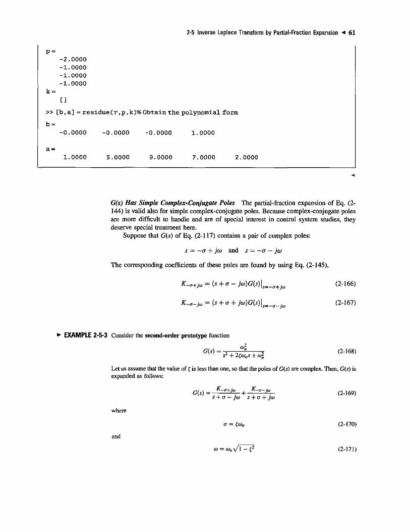
2-5 Inverse Laplace Transform by Partial-Fraction Expansion 61
P = -2 .0000 -1 .0000 -1 .0000 - 1 . 0 0 0 0
k = [ ]
» [b , a] = residue(r, p, k ) % Obtain the polynomial form
b = -0.0000 -0.0000 -0.0000 1.0000
a = 1.0000 5.0000 9.0000 7.0000 2.0000
G(s) Has Simple Complex-Conjugate Poles The partial-fraction expansion of Eq. (2-144) is valid also for simple complex-conjugate poles. Because complex-conjugate poles are more difficult to handle and are of special interest in control system studies, they deserve special treatment here.
Suppose that G(s) of Eq. (2-117) contains a pair of complex poles:
s = —a + jco and s = — a — jco
The corresponding coefficients of these poles are found by using Eq. (2-145),
K-a+jo = (-V + o - ja>)G(s)\s=:_a+.(o (2-166)
K-a-}m = (s + a + jw)G(s) \s=_a_j(0 (2-167)
EXAMPLE 2-5-3 Consider the second-order prototype function 2
G{s) = -, , W" 7 (2-168)
Let us assume that the value of £ is less than one, so that the poles of G(s) are complex. Then, G(s) is expanded as follows:
G(s)= f -*«> + * -* -> (2-169) s + cr — jco s + a + jco
where
rr=?w„ (2-170)
and
w = o , V l - f 2 (2-171)

62 Chapter 2. Mathematical Foundation
The coefficients in Eq. (2-169) are determined as
K-a+j» = (s + 0- ja>)G(s) s=-o+ja>
K-n-jw = (s + <T + jco)G{s)
The complete partial-fraction expansion of Eq. (2-168) is
2jco
_ii 2jco
2ja>
1 1 s + CT — ju) s + a + jco
(2-172)
(2-173)
(2-174)
Taking the inverse Laplace transform on both sides of the last equation gives
g{t)=^-e-°' (eJm - e-jat) t > 0
Or,
*(0 = x/T1?
e-K<»*i S i n W/i ̂ /i _ 5¾ / > o _" 0-Z«>ntei
(2-175)
(2-176)
-~1
2-6 APPLICATION OF THE LAPLACE TRANSFORM TO THE SOLUTION OF LINEAR ORDINARY DIFFERENTIAL EQUATIONS
As we see later, the mathematical models of most components of control systems are represented by first- or second-order differentia] equations. In this textbook, we primarily study linear ordinary differential equations with constant coefficients such as the first-order linear system:
dyit) dl
w{t) = /(0 (2-177)
or the second-order linear system:
d2y{t) , dy{t) t . , , , , «i ^77- + ooyW = / ( 0 dt2
dt (2-178)
Linear ordinary differential equations can be solved by the Laplace transform method with the aid of the theorems on Laplace transform given in Section 2-4, the partial-fraction expansion, and the table of Laplace transforms. The procedure is outlined as follows:
1. Transform the differential equation to the .-.-domain by Laplace transform using the Laplace transform table.
2. Manipulate the transformed algebraic equation and solve for the output variable.
3. Perform partial-fraction expansion to the transformed algebraic equation.
4. Obtain the inverse Laplace transform from the Laplace transform table.
Let us examine two specific cases, first- and second-order prototype systems.
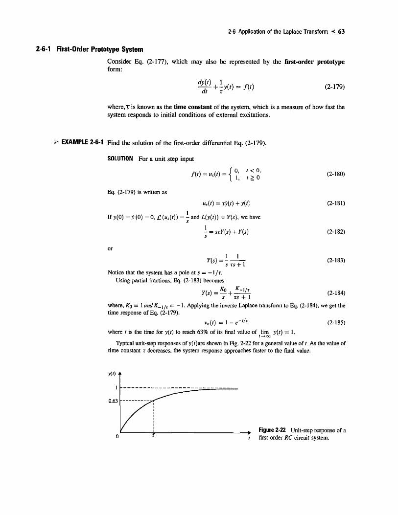
2-6 Application of the Laplace Transform 63
1 First-Order Prototype System
Consider Eq. (2-177), which may also be represented by the first-order prototype form:
at T (2-179)
where, t is known as the time constant of the system, which is a measure of how fast the system responds to initial conditions of external excitations.
EXAMPLE 2-6-1 Find the solution of the first-order differential Eq. (2-179).
SOLUTION For a unit step input
fit) = »,(/) = 0, t < 0, 1. t> 0
Eq. (2-179) is written as
»*(0 = *v(0 + y(t)
If y(0) = y (0) = 0, £ ( K , ( 0 ) = - and L(y(t)) = Y{s), we have
]- = STY(S) + Y(s)
or
Y(s) = 1 1 S TS + 1
Notice that the system has a pole at .v = — 1/T. Using partial fractions, Eq. (2-183) becomes
KQ , tf-i/r Y(s) =
s rs + 1
(2-180)
(2-181)
(2-182)
(2-183)
(2-184)
where, KQ = 1 andK_\ir = - 1 . Applying the inverse Laplace transform to Eq. (2-184), we get the time response of Eq. (2-179).
vJt) =\-e~'/T (2-185)
where t is the time for >•(/) to reach 63% of its final value of lim >'(/) = 1.
Typical unit-step responses of y(|)are shown in Fig. 2-22 for a general value of/. As the value of time constant r decreases, the system response approaches faster to the final value.
^ Figure 2-22 Unit-step response of a t first-order RC circuit system.

64 Chapter 2. Mathematical Foundation
Toolbox 2-6-1
The inverse Laplace transform for Eq. (2-183) is obtained using the MATLAB Symbolic Toolbox by the following sequence of MATLAB functions.
» syms s t a u ; » i l a p l a c e ( l / ( t a u * s A 2 + s ) ) ;
The result is Eq. (2-185).
Note, the sym command lets you construct symbolic variables and expressions, and the command:
» syms s t a u ;
is equivalent to:
» s = s y m ( ' s ' ) ; » t a u = s y m ( ' t a u ' ) ; Time response of Eq. (2-183), shown in Fig. 2-22, for a given value r = 0.1 is obtained using
» c l e a r a l l ; » t = 0 : 0 . 0 1 : 1 ; » t a u = 0 . 1 ; » p l o t ( l - e x p ( - t / t a u ) ) ;
You may wish to confirm that at t = 0.1, y(t) = 0.63.
2-6-2 Second-Order Prototype System
Similarly, for the second-order prototype of the form:
£g>+2(a)/_f+a>ly{l) = m (2.186) where C is known as the damping ratio, and co„ is the natural frequency of the system. The prototype forms of differential equations provide a common format of representing various components of a control system. The significance of this representation will become more evident when we study the time response of control systems in Chapter 5.
EXAMPLE 2-6-2 Consider the differential equation
ijM + 3 m + 2,.(,) =5,,,(,) (2-.87)
where us{l) is the unit-step function. The initial conditions are v(0) = — 1 and y*^(0) = dy(t)/itt\t=(i = 2. To solve the differential equation, we first take the Laplace transform on both sides of Eq. (2-153):
s2Y{s) - sy{0) - v(l' (0) + 3sY{s) - 3y(0) + 2Y(s) = S/s (2-188)
Substituting the values of the initial conditions into the last equation and solving for Y(.s), we get

2-6 Application of the Laplace Transform 65
Eq. (2-189) is expanded by partial-fraction expansion to give
KW4-JTT+2(7^2J (2-190)
Taking the inverse Laplace transform of Eq. (2-190), we get the complete solution as
y(t) =~5e~'+^e~2t t>0 (2-191)
The first term in Eq. (2-191) is the steady-state solution or the particular integral; the last two terms represent the transient or homogeneous solution. Unlike the classical method, which requires separate steps to give the transient and the steady-state responses or solutions, the Laplace transform method gives the entire solution in one operation.
If only the magnitude of the steady-state solution of >'(/) is of interest, the final-value theorem of Eq. (2-133) may be applied. Thus,
lim y(t) = Urn sY(s) = lim f ~* \ = r (2-192)
where, in order to ensure the validity of the final-value theorem, we have first checked and found that the poles of function xY(s) are all in the left-half s-plane.
EXAMPLE 2-6-3 Consider the linear differential equation
^ ^ + 34.5 QQ + iOOOy(f) = 1000^(0 (2-193) at1 at
The initial values of y{t) and dy{t)/dt are zero. Taking the Laplace transform on both sides of Eq. (2-193), and solving for Y(s), we have
w , ) = lM = <£ (2.194) "• ' s(x2 + 34.5* + 1000) s(s2 + Ufas + a%)
where, using the second-order prototype representation, £ = 0.5455 and a>„ = 31.62. The inverse Laplace transform of Eq. (2-194) can be executed in a number of ways. The Laplace transform table in Appendix C provides the time-response expression in Eq. (2-194) directly. The result is
y(t) = l s m ( a j , , y i - j ; 2 / + fl) t>0 (2-195) V W 2 \ • /
where
_i i .. . .o?rrad
Thus.
9 = cos- 1? = 0.9938 radf = 56.94° ——) (2-196)
y(t) = l -1 .193e - 1 7 2 5 r s in (26.5/ + 0.9938) t>0 (2-197)
Eq. (2-197) can be derived by performing the partial-fraction expansion of Eq. (2-194), knowing that the poles are at * = 0, -a + jco, and —a — jco, where
a = ¢0¾ = 17.25 (2-198)
co = con \ / l - f 2 = 26.5 (2-199)

66 Chapter 2. Mathematical Foundation
The partial-fraction expansion of Eq. (2-194) is written
Y(s) = — • • K-a+J° i K-«-)i»
s s + a — jco s + a + jo)
where
KQ = sY(s] = 1 .v = 0
K-o+jco = (S + O - J0))Y{s)
K-a-p, = (s + a + jco)Y(s)
The angle 0 is given by
s = -cr+jco 2 , / \ / l — £ 2
s = -a—jco vV^?
0 = 180° - cos - 'c
and is illustrated in Fig. 2-23. The inverse Laplace transform of Eq. (2-200) is now written
y(t) = l +
= l +
l
2JVl=P ~<<0-'> \pj(cl-<t>) _ *-j{«>t-tf
y/T=? r ^ " ' sinfwhV^ - £ 2 f - 0
Substituting Eq. (2-204) into Eq. (2-205) for 0, we have
1 y(t) = i - , -«W c: -w\ioHy/\ - f 2 < + COS~'< ? > 0
or v(0 = 1 - 1.193e_17-25t sin(26.5f + 0.9938) t > 0
(2-200)
(2-201)
(2-202)
(2-203)
(2-204)
(2-205)
(2-206)
(2-207)
,y-plane
Figure 2-23 Root location in the .v-plane.

2-7 Impulse Response and Transfer Functions of Linear Systems 67
Toolbox 2-6-2
Time response of Eq. (2-194) for a unit-step input may also be obtained using
num= [1000] ; den= [1 34.5 1000] ; G = tf (num, den) ; step(G); title ( ' Step Response ' ) xlabel ('Time (sec') ylabel ( 'Amplitude ' )
Alternatively:
s = tf('s'); G=1000/(sA2+34.5"s+1000); step (G) ; title ( ' Step Response ' ) xlabel ( 'Time(sec ' ) ylabel('Amplitude')
'step" produces the time response of a function for a unit-step input.
Step Response
1.4
1.2 -
0.15 0.2 Time (sec)
0.3 0.35
2-7 IMPULSE RESPONSE AND TRANSFER FUNCTIONS OF LINEAR SYSTEMS
The classical way of modeling linear time-invariant systems is to use transfer functions to represent input-output relations between variables. One way to define the transfer function is to use the impulse response, which is defined as follows.
2-7-1 Impulse Response
Consider that a linear time-invariant system has the input u{t) and output y(t). As shown in Fig. 2-24, a rectangular pulse function u(t) of a very large magnitude «/2s becomes

68 • Chapter 2. Mathematical Foundation
«(fl
t+x - • /
Figure 2-24 Graphical representation an impulse function.
an impulse function for very small durations as e—>0. The equation representing Fig. 2-24 is
u(t) = < u
2>:
0 / < r - e
X -£<t<T + £
0 / > T + £
(2-208)
For u — 1, «(/) = 5(/) is also known as unit impulse or Dirac delta function. For t = 0 in Eq. (2-208), using Eq. (2-116) and noting the actual limits of the integral are defined from / = 0 - to / = oo, it is easy to verify that the Laplace transform of 8(t) is unity, 1.6-45(/)] = 1 ase~»0.
The important point here is that the response of any system can be characterized by its impulse response g(t), which is defined as the output when the input is a unit-impulse function 5(/). Once the impulse response of a linear system is known, the output of the system y(t), with any input, u(t), can be found by using the transfer function. We define
G(s) =
as the transfer function of the system.
£(>>(/)) Y(s)
C[u(t)) F(s) (2-209)
EXAMPLE 2-7-1 For the second-order prototype system Eq. (2-186), shown in Example 2-5-3 as:
Hence, ^ + W ^ + *(0-«2«M
G(s) = cm) _ gg £(«(0) s2 + Z&ns + cof.
(2-210)
(2-211)
is the transfer function of the system in Eq. (2-210). Similar to Example 2-5-3, given zero initial conditions, the impulse response g(t) is
g(t)= -j=±=e-^ s i n ^ v T ^ / > 0 (2-212)

2-7 Impulse Response and Transfer Functions of Linear Systems 69
For a unit-step input u(t) = us{t), using the convolution properties of Laplace transforms,
G(s) = C usg(t - r)dx
From the inverse Laplace transform of Eq. (2-213), the output y(t) is therefore
usg(t - r)dx
(2-213)
,-i<o„i y(t) = 1 - — = = sin Un Jl-ft + d) />0
where, 0 = cos f. . - ]
(2-214)
i
Toolbox 2-7-1
The unit impulse response of Eq. (2-194) may be obtained using
20
-5
n u m = [ 1 0 0 0 ] ; d e n = [ 1 3 4 . 5 1 0 0 0 ] ; G = t f ( n u m . d e n ) ; i m p u l s e ( G ) ;
Alternatively:
s = t f ( ' s ' ) ; G = 1 0 0 0 / ( s A 2 + 3 4 . 5 * s + 1 0 0 0 ) ; i m p u l s e (G) ;
Impulse Response
0.05 0.1 0.15 0.2 0.25 0.3 0.35 0.4 0.45

70 Chapter 2. Mathematical Foundation
2-7-2 Transfer Function (Single-Input, Single-Output Systems)
The transfer function of a linear time-invariant system is defined as the Laplace transform of the impulse response, with all the initial conditions set to zero.
Let G(s) denote the transfer function of a single-input, single-output (SISO) system, with input 2/(/), output ></), and impulse response g(t). The transfer function G(s) is defined as
G(s)=£\g(t)} (2-215)
The transfer function G(s) is related to the Laplace transform of the input and the output through the following relation:
C(,) = m (2.216)
with all the initial conditions set to zero, and Y(s) and U(s) are the Laplace transforms of y(t) and u(t), respectively.
Although the transfer function of a linear system is defined in terms of the impulse response, in practice, the input-output relation of a linear time-invariant system with continuous-data input is often described by a differential equation, so it is more convenient to derive the transfer function directly from the differential equation. Let us consider that the input-output relation of a linear time-invariant system is described by the following //th-order differential equation with constant real coefficients:
i"y(t) ( d"-ly{t) t dy{t an-\ , ' . +••• + «1 — 7 - +«()>'(0 dt" ' ""-1 <ft»-l ' ' "l dt
, d'"u(t) , d'"-[u{t) , du{t) , , . (2-217)
The coefficients OQ, a\, . . . , an-\ and b$. b\, . . . , bm are real constants. Once the input u(t) for t > to and the initial conditions of y{t) and the derivatives of y(i) are specified at the initial time t — to, the output response y(t) for f > to is determined by solving Eq. (2-217). However, from the standpoint of linear-system analysis and design, the method of using differential equations exclusively is quite cumbersome. Thus, differential equations of the form of Eq. (2-217) are seldom used in their original form for the analysis and design of control systems. It should be pointed out that, although efficient subroutines are available on digital computers for the solution of high-order differential equations, the basic philosophy of linear control theory is that of developing analysis and design toots that will avoid the exact solution of the system differential equations, except when computer-simulation solutions are desired for final presentation or verification. In classical control theory, even computer simulations often start with transfer functions, rather than with differential equations.
To obtain the transfer function of the linear system that is represented by Eq. (2-145), we simply take the Laplace transform on both sides of the equation and assume zero initial conditions. The result is
( / - f a , ^ / - 1 + ••• +alS + a0)Y(s) = (b„ls"' + bm-]sm-] + ••• + b\s + bQ)U(s)
(2-218)
The transfer function between u(t) and >'(/) is given by
r , x _ Y(s) _ bmsm + fr,„-i*"'-' + • • • + bis + b0 U[S)-U(s)- s»+an-]^ + ---+a[s + ao U " Z 1 V )

2-7 Impulse Response and Transfer Functions of Linear Systems 71
The properties of the transfer function are summarized as follows:
• The transfer function is defined only for a linear time-invariant system. It is not defined for nonlinear systems.
• The transfer function between an input variable and an output variable of a system is defined as the Laplace transform of the impulse response. Alternately, the transfer function between a pair of input and output variables is the ratio of the Laplace transform of the output to the Laplace transform of the input.
• All initial conditions of the system are set to zero.
• The transfer function is independent of the input of the system.
• The transfer function of a continuous-data system is expressed only as a function of the complex variable s. It is not a function of the real variable, time, or any other variable that is used as the independent variable. For discrete-data systems modeled by difference equations, the transfer function is a function of z when the z-transform is used (refer to Appendix D).
2-7-3 Proper Transfer Functions
The transfer function in Eq. (2-147) is said to be strictly proper if the order of the denominator polynomial is greater than that of the numerator polynomial (i.e., n > m). If n = m, the transfer function is called proper. The transfer function is improper if m>n.
2-7-4 Characteristic Equation
The characteristic equation of a linear system is defined as the equation obtained by setting the denominator polynomial of the transfer function to zero. Thus, from Eq. (2-147), the characteristic equation of the system described by Eq. (2-145) is
s" + an-\s" ' + • • • + axs + a0 = 0 (2-220)
Later we shall show that the stability of linear, single-input, single-output systems is completely governed by the roots of the characteristic equation.
2-7-5 Transfer Function (Multivariable Systems)
The definition of a transfer function is easily extended to a system with multiple inputs and outputs. A system of this type is often referred to as a multivariable system. In a multivariable system, adifferential equation of the form of Eq. (2-145) may be used to describe the relationship between a pair of input and output variables, when all other inputs are set to zero. Because the principle of superposition is valid for linear systems, the total effect on any output due to all the inputs acting simultaneously is obtained by adding up the outputs due to each input acting alone.
In general, if a linear system hasp inputs and q outputs, the transfer function between they'th input and the /th output is defined as
^)=¾ (2-22.) with Rk(s) = 0, k = 1,2,..., p,k^j. Note that Eq. (2-151) is defined with only they'th input in effect, whereas the other inputs are set to zero. When all they? inputs are in action, the /th output transform is written
Us) = G/, (5)/?, (s) + Gi2(s)R2(.s) +••• + Gip(s)Rp(s) (2-222)

72 Chapter 2. Mathematical Foundation
It is convenient to express Eq. (2-152) in matrix-vector form:
Y(,) = G(s)R(s)
where
Y(s) =
is the q x 1 transformed output vector;
R(*) =
LU*)
Ms) Ro(s)
L*p(s)
is the p x 1 transformed input vector; and
\Gn(s) G]2(s)
G2\{s) G22{s) G{s) =
mGqi{s) Gq2(s)
is the q x /? transfer-function matrix.
G\p(s)
G2p(s)
Gqp{s)
(2-223)
(2-224)
(2-225)
(2-226)
2-8 STABILITY OF LINEAR CONTROL SYSTEMS
From the studies of linear differential equations with constant coefficients of SISO systems, we learned that the homogeneous solution that corresponds to the transient response of the system is governed by the roots of the characteristic equation. Basically, the design of linear control systems may be regarded as a problem of arranging the location of the poles and zeros of the system transfer function such that the system will perform according to the prescribed specifications.
Among the many forms of performance specifications used in design, the most important requirement is that the system must be stable. An unstable system is generally considered to be useless.
When all types of systems are considered—linear, nonlinear, time-invariant, and time-varying—the definition of stability can be given in many different forms. We shall deal only with the stability of linear SISO time-invariant systems in the following discussions.
For analysis and design purposes, we can classify stability as absolute stability and relative stability. Absolute stability refers to whether the system is stable or unstable; it is a yes or no answer. Once the system is found to be stable, it is of interest to determine how stable it is, and this degree of stability is a measure of relative stability.
In preparation for the definition of stability, we define the two following types of responses for linear time-invariant systems:
• Zero-state response. The zero-state response is due to the input only; all the initial conditions of the system are zero.

2-9 Bounded-Input, Bounded-Output (BIBO) Stability—Continuous-Data Systems 73
• Zero-input response. The zero-input response is due to the initial conditions only; all the inputs are zero.
From the principle of superposition, when a system is subject to both inputs and initial conditions, the total response is written
Total response = zero-state response + zero-input response
The definitions just given apply to continuous-data as well as discrete-data systems.
2-9 BOUNDED-INPUT, BOUNDED-OUTPUT (BIBO STABILITY—CONTINUOUS-DATA SYSTEMS
Let a(t), y(t), and g(t) be the input, output, and the impulse response of a linear time-invariant system, respectively. With zero initial conditions, the system is said to be BJBO (bounded-input, bounded-output) stable, or simply stable, if its output y(t) is bounded to a bounded input u(t).
The convolution integral relating u(t), y(t), and g(t) is
y(t) = / U(t - T)g{t)dT Jo
Taking the absolute value of both sides of the equation, we get
\y{t)\ = u(t — x)g{x)dx
(2-227)
(2-228)
or
|>.(/)|< / \u(t - x)\\g(x)\dx -/0
If u(t) is bounded,
\u{t)\ < M
where M is a finite positive number. Then,
(2-229)
(2-230)
\}'(t)\<M \g{x)\dx (2-231) Jo
Thus, if y(t) is to be bounded, or
\y(t)\ <N<oc (2-232)
where TV is a finite positive number, the following condition must hold:
M I \g{x)\dx<N<oo Jo
Or, for any finite positive Q,
(2-233)
\g{x)\dx< Q<oo (2-234)

74 Chapter 2. Mathematical Foundation
The condition given in Eq. (2-234) implies that the area under the |#(r)|-versus-T-curve must be finite.
2-10 RELATIONSHIP BETWEEN CHARACTERISTIC EQUATION ROOTS AND STABILITY
To show the relation between the roots of the characteristic equation and the condition in Eq. (2-234), we write the transfer function G(s), according to the Laplace transform definition, as
G(s) = C[g(r)] = [^ g(t)e-sldt (2-235) Jo /0
Taking the absolute value on both sides of the last equation, we have
\G(s)\ = /•oc
/ g{t)e-«dt h)
< i^\g{t)\\e~sl\dt (2-236) ./()
Because \e st \ = \e m\, where a is the real part of s, when s assumes a value of a pole of G(s), G(s) = oc, Eq. (2-236) becomes
/•00
oo < / \g{t)\\e-ot\dt (2-237)
If one or more roots of the characteristic equation are in the right-half .y-plane or on the jco-axis, a > 0, then
\e-n'\<M=\ (2-238)
Eq. (2-237) becomes
o o < f M\g{t)\dt= f \g{t)\dt (2-239) Jo Jo
which violates the BIBO stability requirement. Thus, for BIBO stability, the roots of the characteristic equation, or the poles o/G(s), cannot be located in the right-half "s-plane or on thejoi-axis; in other words, they must all lie in the left-half •s-plane. A system is said to be unstable if it is not BIBO stable. When a system has roots on the /w-axis, say, at s = JCOQ
and s = —JCOQ, if the input is a sinusoid, sin Wgf, then the output will be of the form of t sin coo?, which is unbounded, and the system is unstable.
2-11 ZERO-INPUT AND ASYMPTOTIC STABILITY OF CONTINUOUS-DATA SYSTEMS
In this section, we shall define zero-input stability and asymptotic stability and establish their relations with BIBO stability.
Zero-input stability refers to the stability condition when the input is zero, and the system is driven only by its initial conditions. We shall show that the zero-input stability also depends on the roots of the characteristic equation.
Let the input of an «th-order system be zero and the output due to the initial conditions be y(t). Then, y(t) can be expressed as
«-i >'(t) =J2^(¥k)(h)) (2-240)
k=0

2-11 Zero-Input and Asymptotic Stability of Continuous-Data Systems 75
where
v{k)(t«) = dky(t)
dtk (2-241) t=t<\
(kh and gk(t) denotes the zero-input response due to y (t0). The zero-input stability is defined as follows: If the zero-input response y(t), subject to the finite initial conditions, y<k)(t0), reaches zero as t approaches infinity, the system is said to be zero-input stable, or stable; otherwise, the system is unstable.
Mathematically, the foregoing definition can be stated: A linear time-invariant system is zero-input stable if, for any set of finite y(k)(t0), there exists a positive number M, which depends on y(k)(t0), such that
1. \y(t) | < M < oo for all t > to (2-242)
and
2.
lim \y(t)\ = 0 t -» 30
(2-243)
Because the condition in the last equation requires that the magnitude of y(t) reaches zero as time approaches infinity, the zero-input stability is also known at the asymptotic stability.
Taking the absolute value on both sides of Eq. (2-240), we get
bCOl = / i - i
£s*«.v(A)('o) k=0
<Y,\gk(t)\y{k)(u>) k=0
(2-244)
Because all the initial conditions are assumed to be finite, the condition in Eq. (2-242) requires that the following condition be true:
i>(oi < o o for all/>0 (2-245)
*=o
Let the n characteristic equation roots be expressed as Si = o\ + jcoj, i = 1,2. . . . . n. Then, if m of the n roots are simple, and the rest are of multiple order, y(t) will be of the form:
>'(') i=\
u—m—
/=() &" + Life*' (2-246)
where K, and L,- are constant coefficients. Because the exponential terms eSi' in the last equation control the response y(t) as t —»• oo, to satisfy the two conditions in Eqs. (2-242) and (2-243), the real parts of Sj must be negative. In other words, the roots of the characteristic equation must all be in the left-half .y-plane.
From the preceding discussions, we see that,/or linear time-invariant systems, BIBO, zero-input, and asymptotic stability all have the same requirement that the roots of the characteristic equation must all be located in the left-half s-plane. Thus, if a system is BIBO stable, it must also be zero-input or asymptotically stable. For this reason, we shall simply refer to the stability condition of a linear system as stable or unstable. The latter

76 Chapter 2. Mathematical Foundation
TABLE 2-5 Stability Conditions of Linear Continuous-Data Time-Invariant SISO Systems
Stability Condition Root Values
Asymptotically stable or simply stable a-, < 0 for all / , / = 1 , 2 , . . . , « . (All the roots are in the left-half .v-plane.)
Marginally stable or marginally CT, = 0 for any i for simple roots, and no CTJ > 0 unstable For i = 1. 2, . . . , n (at least one simple root, no
multiple-order roots on the y'&>-axis, and n roots in the right-half 5-plane; note exceptions)
Unstable a; > 0 for any i, or a,- = 0 for any multiple-oidei root; i = 1, 2. . . . , n (at least one simple root in the right-half 5-plane or at least one multiple-order root on the ycy-axis)
condition refers to the condition that at least one of the characteristic equation roots is not in the left-half s-plane. For practical reasons, we often refer to the situation in which the characteristic equation has simple roots on they<w-axis and none in the right-half plane as marginally stable or marginally unstable. An exception to this is if the system were intended to be an integrator (or, in the case of control systems, a velocity control system); then the system would have root(s) at s — 0 and would be considered stable. Similarly, if the system were designed to be an oscillator, the characteristic equation would have simple roots on the yw-axis, and the system would be regarded as stable.
Because the roots of the characteristic equation are the same as the eigenvalues of A of the state equations, the stability condition places the same restrictions on the eigenvalues.
Let the characteristic equation roots or eigenvalues of A of a linear continuous-data time-invariant SISO system be si = o~; + ja>i, i — 1, 2, . . . , n. If any of the roots is complex, it is in complex-conjugate pairs. The possible stability conditions of the system are summarized in Table 2-5 with respect to the roots of the characteristic equation.
The following example illustrates the stability conditions of systems with reference to the poles of the system transfer functions that are also the roots of the characteristic equation.
EXAMPLE 2-11-1 The following closed-loop transfer functions and their associated stability conditions are given.
20 M(s) = - -r- —-. — BIBO or asymptotically stable (or, simply, stable)
(5+1)(5 + 2)(5 + 3)
20(5+1) (5-1)(52 +25+ 2) M(s) = 7 iw 2 i "»—T̂ T Unstable due to the pole at s = 1
M(s) = -. ^ . — Marginally stable or marginally unstable due to s = ±j2 (s + 2)(5^ +4)
M(s) = ~ Unstable due to the multiple-order pole at s = ± /2 (.v2+4)2(5+10)
M(s) = —. 5 ~ — Stable if the pole at s = 0 is placed intentionally W 54 + 3053 + 52 + 105 F F J

2-12 Methods of Determining Stability 77
2-12 METHODS OF DETERMINING STABILITY
The discussions in the preceding sections lead to the conclusion that the stability of linear time-invariant SISO systems can be determined by checking on the location of the roots of the characteristic equation of the system. For all practical purposes, there is no need to compute the complete system response to determine stability. The regions of stability and instability in the .v-plane are illustrated in Fig, 2-25. When the system parameters are all known, the roots of the characteristic equation can be found using MATLAB as demonstrated in various MATLAB Toolbox windows discussed earlier in this chapter. The Transfer Function Symbolic Tool (tfsym) developed for this chapter may also be utilized to find the transfer function poles and zeros. See the end of this chapter for some examples. These programs are discussed in detail in Appendix G. For design purposes, there will be unknown or variable parameters imbedded in the characteristic equation, so a Routh-Hurwitz stability routine has also been developed for this textbook (tfrouth), which is discussed at the end of this chapter.
The methods outlined in the following list are well known for determining the stability of linear continuous-data systems without involving root solving.
1. Routh-Hurwitz criterion. This criterion is an algebraic method that provides information on the absolute stability of a linear time-invariant system that has a characteristic equation with constant coefficients. The criterion tests whether any of the roots of the characteristic equation lie in the right-half .v-plane. The number of roots that lie on they'w-axis and in the right-half .v-plane is also indicated.
2. Nyquist criterion. This criterion is a semi-graphical method that gives information on the difference between the number of poles and zeros of the closed-loop transfer function that are in the right-half .v-plane by observing the behavior of the Nyquist plot of the loop transfer function. This topic is discussed in detail in Chapter 8, and the concepts of loop transfer function and close-loop systems are discussed in Chapter 3.
3. Bode diagram. This diagram is a plot of the magnitude of the loop transfer function G(jto)H{jco) in dB and the phase of G(jo))H(jco) in degrees, all versus frequency co- The concepts of loop transfer function and closed-loop systems are
Stable region
Stable region
J(0
0
,s-plane
Unstable region
Unstable region
a
Figure 2-25 Stable and unstable regions in the .v-plane.

78 Chapter 2. Mathematical Foundation
discussed in Chapter 3. The stability of the closed-loop system can be determined by observing the behavior of these plots. This topic is discussed in detail in Chapter 8.
Thus, as will be evident throughout the text, most of the analysis and design techniques on control systems represent alternate methods of solving the same problem. The designer simply has to choose the best analytical tool, depending on the particular situation.
Details of the Routh-Hurwitz stability criterion are presented in the following section.
2-13 ROUTH-HURWITZ CRITERION
The Routh-Hurwitz criterion represents a method of determining the location of zeros of a polynomial with constant real coefficients with respect to the left half and right half of the s-plane, without actually solving for the zeros. Became root-finding computer programs can solve for the zeros of a polynomial with ease, the value of the Routh-Hurwitz criterion is at best limited to equations with at least one unknown parameter.
Consider that the characteristic equation of a linear time-variant SISO system is of the form
F(s) = ans" + a,,-].?"-1 + • • • + a\s + a0 = 0 (2-247)
where all the coefficients are real. To ensure the last equation does not have roots with positive real parts, it is necessary (but not sufficient) that the following conditions hold:
1. All the coefficients of the equation have the same sign.
2. None of the coefficients vanish.
These conditions are based on the laws of algebra, which relate the coefficients of Eq. (2-247) as follows:
flfi-1 = - ^ a l l roots (2-248)
= y ^ products of the roots taken two at a time (2-249)
On-3 = - V^ products of the roots taken three at a time (2-250)
^ = ( - 1 )"products of all the roots (2-251) an
Thus, all these ratios must be positive and nonzero unless at least one of the roots has a positive real part.
The two necessary conditions for Eq. (2-247) to have no roots in the right-half j-plane can easily be checked by inspection of the equation. However, these conditions are not sufficient, for it is quite possible that an equation with all its coefficients nonzero and of the same sign still may not have all the roots in the left half of the 5-plane.

2-13 Routh-Hurwitz Criterion < 79
2-13-1 Routh's Tabulation
The Hurwitz criterion gives the necessary and sufficient condition for all roots of Eq. (2-247) to lie in the left half of the s-plane. The criterion requires that the equation's n Hurwitz determinants must all be positive.
However, the evaluation of the n Hurwitz determinants is tedious to carry out. But Routh simplified the process by introducing a tabulation method in place of the Hurwitz determinants.
The first step in the simplification of the Hurwitz criterion, now called the Routh-Hurwitz criterion, is to arrange the coefficients of the equation in Eq. (2-247) into two rows. The first row consists of the first, third, fifth, . . . , coefficients, and the second row consists of the second, fourth, sixth, . . . , coefficients, all counting from the highest-order term, as shown in the following tabulation:
a„ an~2 (1),-4 a„-6 • • •
«M-1 « M - 3 a,i-5 O-n-1 - - -
The next step is to form the following array of numbers by the indicated operations, illustrated here for a sixth-order equation:
a6s6 + a5s
5 + ••• + a\ s + tfo = 0 (2-252)
/
s5
s4
? 3 i j
s2
sl
s°
«6
«5
a5a4 - «6«3 _
«5
Acii - a<,B ^
A BC-AD „
c ~E
ED - Cao r
E =F
Fao - E x 0 T; = «o
«4
m asai -a6ai
= ts «5
Aa\ - a5ao _ A
CciQ-AxO c =ao
0
0
«2
a i
a^ciQ — «6 x 0 = fl()
«5
A x O - f l ^ x O — 0 A U
CxO-AxO C
0
0
" 0
0
0
0
0
0
0 F
This array is called the Routh's tabulation or Routh's array. The column of s's on the left side is used for identification purposes. The reference column keeps track of the calculations, and the last row of the Routh's tabulation should always be the s row.
Once the Routh's tabulation has been completed, the last step in the application of the criterion is to investigate the signs of the coefficients in the first column of the tabulation, which contains information on the roots of the equation. The following conclusions are made:
The roots of the equation are all in the left half of the .s-plane if all the elements of the first column of the Routh's tabulation are of the same sign. The number of changes of signs in the elements of the first column equals the number of roots with positive real parts, or those in the right-half .v-plane.

80 Chapter 2. Mathematical Foundation
The following examples illustrate the applications of the Routh-Hurwitz criterion when the tabulation terminates without complications.
EXAMPLE 2.13.1 Consider the equation
2.v4 + s3 + 3 r + 55 + 10 = 0 (2-253)
Because the equation has no missing terms and the coefficients are all of the same sign, it satisfies the necessary condition for not having roots in the right-half or on the imaginary axis of the .y-plane. However, the sufficient condition must still be checked. Routh's tabulation is made as follows:
Sign change
Sign change
.s4
J3
i 5"
Sl
,°
2
1
(1)(3)-(2)(5) ]
(-7)(5)-(1)(10)
-7
10
-7
-- 6.43
3
5
10
0
0
10
0
0
0
0
Because there are two sign changes in the first column of the tabulation, the equation has two roots in the right half of the .y-plane. Solving for the roots of Eq. (2-253), we have the four roots at s = -1.005 ± /0.933 and s = 0.755 ± j 1.444. Clearly, the last two roots are in the right-half .y-plane, which cause the system to be unstable.
Toolbox 2-13-1
The roots of the polynomial in Eq. (2-253) are obtained using the following sequence of MATLAB functions.
» clear all » p = [2 1 3 5 10] % Define polynomial 2*sA4+sA3+3*sA2+5*s+10
P = 2 1 3 5 10
» roots(p) ans =
0.7555 + 1.4444i 0.7555 - 1.44441 -1.0055 + 0.93311 -1.0055 - 0.93311
2-13-2 Special Cases when Routh's Tabulation Terminates Prematurely
The equations considered in the two preceding examples are designed so that Routh's tabulation can be carried out without any complications. Depending on the coefficients of the equation, the following difficulties may occur, which prevent Routh's tabulation from completing properly:

2-13 Routh-Hurwitz Criterion 81
1. The first element in any one row of Routh's tabulation is zero, but the others are not.
2. The elements in one row of Routh's tabulation are all zero.
In the first case, if a zero appears in the first element of a row, the elements in the next row will all become infinite, and Routh's tabulation cannot continue. To remedy the situation, we replace the zero element in the first column by an arbitrary small positive number B, and then proceed with Routh's tabulation. This is illustrated by the following example.
EXAMPLE 2-13-2 Consider the characteristic equation of a linear system
sA + s3 + 2s2 + 2,y + 3 = 0 (2-254)
Because all the coefficients are nonzero and of the same sign, we need to apply the Routh-Hurwitz criterion. Routh's tabulation is carried out as follows:
.v4 1 2 3
s3 1 2 0
.v2 0 3
Because the first element of the $ row is zero, the elements in the A*1 row would all be infinite. To overcome this difficulty, we replace the zero in the s" row with a small positive number c, and then proceed with the tabulation. Starting with the s2 row, the results are as follows:
S2 £ 3
„. , i 2c-3 3 „ Sign change r S — 0
s c Sign change s° 3 0
Because there are two sign changes in the first column of Routh's tabulation, the equation in Eq. (2-254) has two roots in the right-half s-plane. Solving for the roots of Eq. (2-254), we get s = -0.091 ± ./0.902 and s = 0.406 ± yl.293; the last two roots are clearly in the right-half .?-plane.
It should be noted that the c-method described may not give correct results if the equation has pure imaginary roots.
In the second special case, when all the elements in one row of Routh's tabulation are zeros before the tabulation is properly terminated, it indicates that one or more of the following conditions may exist:
1. The equation has at least one pair of real roots with equal magnitude but opposite signs.
2. The equation has one or more pairs of imaginary roots.
3. The equation has pairs of complex-conjugate roots forming symmetry about the origin of the .v-plane; for example, s — — 1 ± j \ , s = 1 ± / 1 .
The situation with the entire row of zeros can be remedied by using the auxiliary equation A(s) = 0, which is formed from the coefficients of the row just above the row of zeros in Routh's tabulation. The auxiliary equation is always an even polynomial; that is, only even powers of .v appear. The roots of the auxiliary equation also satisfy the original equation. Thus, by solving the auxiliary equation, we also get some of the roots of the original equation. To continue with Routh's tabulation when a row of zero appears, we conduct the following steps:
1. Form the auxiliary equation A[s) = 0 by using the coefficients from the row just preceding the row of zeros.
2. Take the derivative of the auxiliary equation with respect to s; this gives dA{s)/ds = 0.

82 Chapter 2. Mathematical Foundation
3. Replace the row of zeros with the coefficients of dA($)/ds — 0.
4. Continue with Routh's tabulation in the usual manner with the newly formed row of coefficients replacing the row of zeros.
5 . Interpret the change of signs, if any, of the coefficients in the first column of the Routh's tabulation in the usual manner. ,
EXAMPLE 2.13.3 Consider the following equation, which may be the characteristic equation of a linear control system:
,v5 + 4 / + 8.v3 + 8s2 + 75 + 4 = 0 (2-255)
Routh's tabulation is
s5 1 8 7 .v4 4 8 4 53 6 6 0 .v2 4 4 .v1 0 0
Because a row of zeros appears prematurely, we form the auxiliary equation using the coefficients of the s2 row:
A{s) = 4s2+4 = 0 (2-256) The derivative of A(s) with respect to s is
^ 1 = & = 0 (2-257) ds
from which the coefficients 8 and 0 replace the zeros in the .v1 row of the original tabulation. The remaining portion of the Routh's tabulation is
.v 8 0 coefficients of dA(s) Ids s° 4
Because there are no sign changes in the first column of the entire Routh's tabulation, the equation in Eq. (2-257) does not have any root in the right-half 5-plane. Solving the auxiliary equation in Eq. (2-256), we get the two roots at .v = j and s = —j, which are also two of the roots of Eq. (2-255). Thus, the equation has two roots on theyoj-axis, and the system is marginally stable. These imaginary roots caused the initial Routh's tabulation to have the entire row of zeros in the 51 row.
Because all zeros occurring in a row that corresponds to an odd power of s creates an auxiliary equation that has only even powers of s, the roots of the auxiliary equation may all lie on theya>-axis. For design purposes, we can use the all-zero-row condition to solve for the marginal value of a system parameter for system stability. The following example illustrates the realistic value of the Routh-Hurwitz criterion in a simple design problem.
EXAMPLE 2-13-4 Consider that a third-order control system has the characteristic equation
53 + 3408.3^2 + 1,204; 0 0 % + 1.5 x 10⁷K = 0 (2-258) The Routh-Hurwitz criterion is best suited to determine the critical value of K for stability, that is, the value of tf for which at least one root will lie on the/&>-axis and none in the right-half s-plane. Routh's tabulation of Eq. (2-258) is made as follows:
53 1 1,204,000
s2 3408.3 l.5xl(?K
, 410.36 x 10⁷ - 1.5 x W1 K V 34083 °
s° 1.5 x 10 7 A:

2-13 Routh-Hurwitz Criterion 83
Toolbox 2-13-2
Refer to Section 2-14-2 for the MATLAB symbolic tool to solve this problem.
For the system to be stable, all the roots of Eq. (2-258) must be in the left-half .v-plane, and, thus, all the coefficients in the first column of Routh's tabulation must have the same sign. This leads to the following conditions:
410.36 x 10⁷ - 1.5 x lO'K „ , „ _ ^ 7 7 ^ > 0 (2-259) 3408.3
and
1.5xl07AT>0 (2-260)
From the inequality of Eq. (2-259), we have K < 273.57, and the condition in Eq. (2-260) gives K > 0. Therefore, the condition of K for the system to be stable is
0<K< 273.57 (2-261) If we let K = 273.57, the characteristic equation in Eq. (2-258) will have two roots on the jco-axis. To find these roots, we substitute K — 273.57 in the auxiliary equation, which is obtained from Routh's tabulation by using the coefficients of the ^2 row. Thus,
A(s) = 3408.352 + 4.1036 x 109 = 0 (2-262)
which has roots at s = /1097 and s = — ./1097, and the corresponding value of K at these roots is 273.57. Also, if the system is operated withiT = 273.57, the zero-input response of the system will be an undamped sinusoid with a frequency of 1097.27 rad/sec.
EXAMPLE 2.13.5 As another example of using the Routh-Hurwitz criterion for simple design problems, consider that the characteristic equation of a closed-loop control system is
53 + 3/¾2 + (K + 2)s + 4 = 0 (2-263)
It is desired to find the range of K so that the system is stable. Roulh's tabulation of Eq. (2-263) is
s3 1 K + 2 s2 3K 4
, 3K(K + 2 ) - 4 3K
s° 4
0
From the .92 row, the condition of stability is K > 0, and from the s1 row, the condition of stability is
3AT2 + 6A' - 4 > 0 (2-264) or
K < - 2.528 or K> 0.528 (2-265)
Toolbox 2-13-3
Refer to Section 2-14-2 for the MATLAB symbolic tool to solve this problem.

84 Chapter 2. Mathematical Foundation
When the conditions of K > 0 and K > 0.528 are compared, it is apparent that the latter requirement is more stringent. Thus, for the closed-loop system to be stable, K must satisfy
K > 0.528 (2-266)
The requirement of K < - 2.528 is disregarded because K cannot be negative. It should be reiterated that the Routh-Hurwitz criterion is valid only if the characteristic equation
is algebraic with real coefficients. If any one of the coefficients is complex, or if the equation is not algebraic, for example, containing exponential functions or sinusoidal functions of s, the Routh-Hurwitz criterion simply cannot be applied.
Another limitation of the Routh-Hurwitz criterion is that it is valid only for the determination of roots of the characteristic equation with respect to the left half or the right half of the s-plane. The stability boundary is the/oi-axis of the s-plane. The criterion cannot be applied to any other stability boundaries in a complex plane, such as the unit circle in the ;-plane, which is the stability boundary of discrete-data systems (Appendix H).
2-14 MATLAB TOOLS AND CASE STUDIES
2-14-1 Description and Use of Transfer Function Tool
If you have access to the MATLAB Symbolic Toolbox, you may use the ACSYS Transfer Function Symbolic Tool by pressing the appropriate button in the ACSYS window or by typing in tfsym in the MATLAB command window. The Symbolic Tool window is shown in Fig. 2-26. Click the "Help for 1st Time User" button to see the instructions on how to use the toolbox. The instructions appear in a Help Dialog window, as shown in Fig. 2-27. As instructed, press the "Transfer Function and Inverse Laplace" button to run the program. You must run this program within the MATLAB command window. Enter the transfer function, as shown in Fig. 2-28, to get the time response.
Stale-Space with I nit. Cond.
Close and Exit
Figure 2-26 The Transfer Function Symbolic window.
i Help Dialog -In] xi
You must have access to MATLAB Symbolic Toolbox. To run Programs, go to MATLAB Command window after clicking each pushbutton.
OK
Figure 2-27 The Symbolic Help Dialog window.

2-14 MATLAB Tools and Case Studies 85
Transfer Function Symbolic. © Kuo & Golnaraghi 8th Edition, John Wiley & Sons, e.g.. Use the following input format: (s+2)*(sA3+2*s+l )/(s*(sA2+2*s+l))
Enter G=5*(s+0.6)/((s+l)*(s+2)*(s+3))
5s+3 (s+ij"(s'+2J"(s+T)
G in polynomial form:
Transfer function:
5s+3 sA3"+6s'AT+iTs+6
G factored:
Zero/pole/gain:
5(s+0.6) ("s+3)"(s+2J"(s+I")
Inverse Laplace transform:
Gtime =
-exp(-t)+7*exp(-2*t)-6*exp(-3*t)
Figure 2-28 The inverse Laplace transform of Eq. (2-267) for an impulse input, in the MATLAB command window.
EXAMPLE 2-14-1 Find the inverse Laplace transform of the transfer function
5s + 3 5s+ 3 G(s) =
[s +1)(5 + 2 ) 0 + 3) s* + 6s2 + 1 Is + 6 (2-267)
You can do this either by using the ilaplace command in the MATLAB command window, as we demonstrated in Toolbox 2-5-1 for Example 2-5-1, or by utilizing the tfsvm function, as shown in Fig. 2-28.
To find the time representation of Eq. (2-267) for a different input function such as a step or a sinusoid, the user may combine the input transfer function (e.g. lis for a unit-step input) with the transfer function in the TFtool input window. So to obtain Eq. (2-267) time representation for a unit-step input, use the following transfer function:
G(s) = 5s+ 3
s{s+l)(s + 2)(s + 3) (2-268)
and repeat the previous steps. Similarly, for the transfer function
Y(s) = 1000
s(s2 + 34.5s + 1000) 0 2 4- 2C*;„.y + a%) (2-269)
using the tfsym tool, the time representation of this system is obtained as 1 + ( - 1 / 2 + 13/40*/)*exp((-69/4-53/27))7 + ( - 1 / 2 - 13/407)* exp((-69/4+
53/27-)7}
2-14-2 MATLAB Tools for Stability
The easiest way to assess stability of known transfer functions is to find the location of the poles. For that purpose, the MATLAB code that appears in Toolbox 2-13-1 is the easiest

86 Chapter 2. Mathematical Foundation
way for finding the roots of the characteristic equation polynomial—i.e., the poles of the system. However, many of the other tools within ACSYS software may also be used to find the poles of the closed-loop system transfer function, including the "Transfer Function Symbolic" (tfsym) and the "Transfer Function Calculator" (tfcal). You may also conduct a more thorough stability study of your system using the root locus and phase and gain margin concepts utilizing the "Controller Design Tool," respectively. These topics will be thoroughly discussed in Chapter 9.
In this section, we introduce the tfrouth tool, which may be used to find the Routh array, and more importantly it may be utilized for controller design applications where it is important to assess the stability of a system for a controller gain, say k.
The steps involved in setting up and then solving a given stability problem using tfrouth are as follows.
1. Type "tfrouth" in the MATLAB command module within the "tfsymbolic" directory.
2. Enter the characteristic polynomial in symbolic (e.g., sA3+sA2+s+1) or in vectorial (e.g. [1 1 1 1]) forms.
3. Press the "Routh-Hurwitz" button and check the results in the MATLAB command window.
4. In case you wish to assess the stability of the system for a design parameter, enter it in the box designated as "Enter Symbolic Parameters." For example, for sA3 + kl*sA2 + k2*s + 1, you need to enter "kl k2" in the "Enter Symbolic Parameters" box, followed by entering the polynomial sA3 + kl*sA2 + k2*s+1 in the "Characteristic Equation" box.
5. Press the "Routh-Hurwitz" button to form the Routh table and conduct the Routh-Hurwitz stability test.
To better illustrate how to use tfrouth, let us solve some of the earlier examples in this chapter.
EXAMPLE 2-14-2 Recall Example 2-13-1; let's use tfrouth for the following polynomial:
2s4 + 53 + 3s2 + 5s + 10 = 0 (2-270)
In the MATLAB command module, type in "tfrouth" and enter the characteristic Eq. (2-270) in polynomial form, followed by clicking the "Roulh-Hurwilz" button to get the Routh-Hurwitz matrix, as shown in Fig. 2-29.
The results match Example 2-14-2. The system is therefore unstable because of two positive poles. The Routh's array first column also shows two sign changes to confirm this result. To see the complete Routh table, the user must refer to the MATLAB command window, as shown in Fig. 2-30.
EXAMPLE 2-14-3 Consider Example 2-13-2 for characteristic equation of a linear system:
.v4 + s3 + 2s2 + 2s + 3 = 0 (2-271)
After entering the transfer function characteristic equation using tfrouth and pressing the "Routh-Hurwitz" button, we get the results shown in Fig. 2-31.
As a result, because of the final two sign changes, we expect to see two unstable poles.
EXAMPLE 2-14-4 Revisiting Example 2-13-3, use tfrouth to study the following characteristic equation:
s5 + 4y4 -I- 8s3 + 8 r + 75 + 4 = 0 (2-272) to get the results shown in Fig. 2-32.

2-14 MATLAB Tools and Case Studies 87
I o 11¾ \t a T Routh Hurwitz
r-Enter Characteristic Equation: •
Enter the characteristic equation using a vector of polynomial coefficients, or in symbolic form with complex variable's'. Enter ALL symbolic parameters in the box labeled 'Enter Symbolic Parameters/
ex: For (sA2 + 3*kp*s + kiA2): enter ' [1, 3*kp, kiA2]' in the Characteristic Equation box and 'kp ki' in the symbolic variables text box.
OR: Type in (sA2 + 3*kp*s + kiA2) in the Characteristic Equation box and 'kp ki' in the symbolic variables text box.
ex: The following are all equivalent: '(sA2 + 7*s +12), [1 7121, and (s+4)*(s+3)'.
Enter Symbolic Parameters (For example:)
Characteristic Equation
2*sA4+sA3+3*sA2+S*s+10
Routh-Hurwitz
Figure 2-29 Entering characteristic polynomial for Example 2-14-2 using the tfrouth module.
Routh-Hurwitz Matrix:
[2 [ fl [ [-7 1 [45/7
I [10
3
5
10
0
0
10 ]
0 ]
0 ]
0 ]
0 ]
There are two sign changes in the first column.
Figure 2-30 Stability results for Example 2-14-2, after using the Routh-Hurwitz test.

88 Chapter 2. Mathematical Foundation
First element of row3 is zero. Epsilon is used. Routh-Hurwitz Matrix:
[ 1 2 3 ]
[ 1 2 0 ]
[ eps 3 0 ]
[-3 + 2 eps ] [ o 0 ]
I eps ]
[ 3 0 0 ]
There are two sign changes in the first column.
Figure 2-31 Stability results for Example 2-14-3, after using the Routh-Hurwitz test.
Row of zeros found at row5 Routh-Hurwitz Matrix:
[1 i L [4 f
1 (6 t I [4 r
[8 r l [4
Auxiliary polynomial is used.
8
8
6
4
0
0
7
4
0
0
0
0
There are two sign changes in the first c
] 1 ] ] 1 J ] 1 J
1 1 J ] 1 J ]
olumn.
Figure 2-32 Stability results for Example 2-14-4, after using the Routh-Hurwitz test.
In this case, the program has automatically replaced the whole row of zeros in the fifth row with the coefficients of the polynomial formed from the derivative of an auxiliary polynomial formed from the fourth row. As a result, the system is unstable. Further, because of the final zero sign changes, we expect to see no additional unstable poles. The unstable poles of the system may be obtained directly by obtaining the roots of the auxiliary polynomial:
A (s) = 4 ^ 4 - 4 = 0 (2-273)
EXAMPLE 2-14-5 Considering the characteristic equation of a closed-loop control system
s3 + 3Ks2 + (K + 2)s + 4 = 0 (2-274)
It is desired to find the range of AT so that the system is stable. See Figs. 2-33,2-34, and 2-35 for more details.
In the end, the user is encouraged to make use of the software to solve examples and problems appearing in this chapter.

2-14 MATLAB Tools and Case Studies 89
Routh Hurwitz
• Enter Characteristic Equation: •
Enter the characteristic equation using a vector of polynomial coefficients, or in symbolic form with complex variable's'. Enter ALL symbolic parameters in the box labeled 'Enter Symbolic Parameters.'
ex: For (sA2 + 3*kp*s + kiA2): enter '[1, 3*kp, kiA2]' in the Characteristic Equation box and 'kp ki" in the symbolic variables text box.
OR: Type in (sA2 + 3*kp*s + kiA2) in the Characteristic Equation box and 'kp ki' in the symbolic variables text box.
ex: The following are all equivalent: '(sA2 + 7*s +12), [1 712], and (s+4)*(s+3)'.
Enter Symbolic Parameters (For example:)
Characteristic Equation
sA3+3*k*sA2+(k+2)*s+4
Routh-Hurwitz
Close
Figure 2-33 Entering characteristic polynomial for Example 2-14-5 using the tfrouth module.
Routh-Hurwitz Matrix:
1 k + 2
3 k 4
- 4 + 3 k + 6 k (1/3 fi
le
4 0
Figure 2-34 The Routh's array for Example 2-14-5.

90 Chapter 2. Mathematical Foundation
» k=.4; » R H
RH =
I I, f 3*k, [ l/3*(-4+3*kA2+6*k)/k, 1 4,
» eval(RH)
ans =
1.0000 1.2000
-0.9333 4.0000
2.4000 4.0000
0 0
There are two sign changes
» k = l ;
» eval(RH)
ans =
1.0000 3.0000 1.6667 4.0000
3.0000 4.0000
0 0
k+2 4 0 0
] ] ] ]
n the first column.
There are no sign changes in the first column.
Figure 2-35 The Routh's array for Example 2-14-5.
2-15 SUMMARY
In this chapter, we presented some fundamental mathematics required for the study of linear control systems. Specifically, we started with complex numbers and their basic properties leading to frequency domain mathematics and plots. The Laplace transform is used for the solution of linear ordinary differential equations. This transform method is characterized by first transforming the real-domain equations into algebraic equations in the transform domain. The solutions are first obtained in the transform domain by using the familiar methods of solving algebraic equations. The final solution in the real domain is obtained by taking the inverse transform. For engineering problems, the transform tables and the partial-fraction expansion method are recommended for the inverse transformation.
In this chapter, the definitions of BIBO, zero-input, and asymptotic stability of linear time-invariant continuous-data and discrete-data systems are given. It is shown that the condition of these types of stability is related directly to the roots of the characteristic equation. For a continuous-data system to be stable, the roots of the characteristic equation must all be located in the left half of the 5-plane.
The necessary condition for a polynomial F(s) to have no zeros on the /&>-axis and in the right half of the .y-plane is that all its coefficients must be of the same sign and none can vanish. The necessary and sufficient conditions of F(s) to have zeros only in the left half of the 5-plane are checked with the Routh-Hurwitz criterion. The value of the Routh-Hurwitz criterion is diminished if the characteristic equation can be solved using MATLAB.

Review Questions 91
REVIEW QUESTIONS
1. Give the definitions of the poles and zeros of a function of the complex variable s.
2. What are the advantages of the Laplace transform method of solving linear ordinary differential equations over the classical method?
3. What are state equations?
4. What is a causal system?
5. Give the defining equation of the one-sided Laplace transform.
6. Give the defining equation of the inverse Laplace transform.
7. Give the expression of the final-value theorem of the Laplace transform. What is the condition under which the theorem is valid?
8. Give the Laplace transform of the unit-step function, us(t).
9. What is the Laplace transform of the unit-ramp function, tu&{t)l
10. Give the Laplace transform of ft) shifted to the right (delayed) by Tfi in terms of the Laplace transform of f(l), F(s).
11. If C[fi(t)] = Fi(s) and £[/2(/)] = F2{s), then find C[f\(t)\ f2(t)\ in terms of F, (s) and F2(s).
12. Do you know how to handle the exponential term in performing the partial-fraction expansion of
F(s) = (*+1)(5 + 2)
13. Do you know how to handle the partial-fraction expansion of a function whose denominator order is not greater than that of the numerator, for example,
\0(s2+5s+l) F(s) =
(*+l)(5 + 2)
14. In trying to find the inverse Laplace transform of the following function, do you have to perform the partial-fraction expansion?
F(s) = ' s + 5)3
15. Can the Routh-Hurwitz criterion be directly applied to the stability analysis of the following systems?
(a) Continuous-data system with the characteristic equation
s4 + 5.v3 + 2s2 +3s + 2e~2s = 0
(b) Continuous-data system with the characteristic equation
.v4 - 5.v3 + 3 r + Ks + K2 = 0
16. The first two rows of Routh's tabulation of a third-order system are
.v3 2 2 s2 4 4
Select the correct answer from the following choices:
(a) The equation has one root in the right-half .y-plane.
(b) The equation has two roots on the y'w-axis at s = j and —j. The third root is in the left-half .v-plane.
92 Chapter 2. Mathematical Foundation
(c) The equation has two roots on the yew-axis at .v = 2j and 5 = —2j. The third root is in the left-half .-plane.
(d) The equation has two roots on the jco-axh at . = 2j and s = -2j. The third root is in the right-half .-plane.
17. If the numbers in the first column of Routh's tabulation turn out to be all negative, then the equation for which the tabulation is made has at least one root not in the left half of the 5-plane. (T) (F)
18. The roots of the auxiliary equation, A (.) = 0, of Routh's tabulation of a characteristic equation must also be the roots of the latter. (T) (F)
19. The following characteristic equation of a continuous-data system represents an unstable system because it contains a negative coefficient.
20. The following characteristic equation of a continuous-data system represents an unstable system because there is a zero coefficient.
. 3 + 5 . 2 + 4 = 0 d ) (F)
21. When a row of Routh's tabulation contains all zeros before the tabulation ends, this means that the equation has roots on the imaginary axis of the .-plane. (T) (F)
Answers to these review questions can be found on this book's companion Web site: www.wiIey.com/college/golnaraghi.
REFERENCES
Complex Variables, Laplace Transforms
1. F. B. Hildebrand, Methods of Applied Mathematics, 2nd Ed., Prentice Hall, Englewood Cliffs, NJ, 1965. 2. B. C. Kuo, Linear Networks and Systems, McGraw-Hill Book Company, New York, 1967. 3. C. R. Wylie, Jr., Advanced Engineering Mathematics, 2nd Ed., McGraw-Hill Book Company, New York,
1960. 4. K. Ogata, Modern Control Engineering, 4th ed., Prentice-Hall, NJ, 2002. 5. J. J. Distefano, A. R. Stubberud, and I. J. Williams, Feedback and Control Systems, 2nd ed., McGraw-Hill,
1990. 6. "ChE-400: Applied Chemical Engineering Calculations," http://www.ent.ohiou.edu/che/che400/Handouts%
20and%20Class%20notes.htm.
Partial-Fraction Expansion
Additional References
7. C. Pottle, "On the Partial Fraction Expansion of a Rational Function with Multiple Poles by Digital Computer," IEEE Trans. Circuit Theory, Vol. CT-tl, pp. 161-162, Mar. 1964.
8. B. 0 . Watkins, "A Partial Fraction Algorithm," IEEE Trans. Automatic Control, Vol. AC-16, pp. 489-491, Oct. 1971.
9. W. J. Palm, 111, Modeling, Analysis, and Control of Dynamic Systems, 2nd Ed., John Wiley & Sons, New York, 1999.
10. K. Ogata, Modern Control Engineering, 4th Ed., Prentice Hall, NJ, 2002. 11. I. Cochin and W. Cadwallender, Analysis and Design of Dynamic Systems, 3rd Ed., Addison-Wesley, 1997. 12. A. Esposito, Fluid Power with Applications, 5th Ed. Prentice Hall, NJ, 2000. 13. H. V. Vu and R. S. Esfandiari, Dynamic Systems, Irwin/McGraw-Hill, 1997. 14. J. L. Shearer, B. T. Kulakowski, and J. F. Gardner, Dynamic Modeling and Control of Engineering Systems,
2nd Ed., Prentice Hall, NJ, 1997. 15. R. L. Woods and K. L. Lawrence, Modeling and Simulation of Dynamic Systems, Prentice Hall, NJ, 1997.

Problems 93
Stability
PROBLEMS
16. B. C. Kuo, Automatic Control Systems, 7th Ed., Prentice Hall, NJ, 1995. 17. B. C. Kuo and F. Golnaraghi, Automatic Control Systems, 8th Ed., John Wiley and Sons, NY, 2003.
18. F. R. Gantmacher, Matrix Theory, Vol. II, Chelsea Publishing Company, New York, 1964. 19. K. J. Khatwani, "On Routh-Hurwitz Criterion," IEEE Trans. Automatic Control, Vol. AC-26, p. 583,
April 1981. 20. S. K. Pillai, "The s Method of the Routh-Hurwitz Criterion," IEEE Trans. Automatic Control,
Vol. AC-26, 584, Aprill981.
PROBLEMS FOR SECTION 2-1 2-1. Find the poles and zeros of the following functions (including the ones at infinity, if any). Mark the finite poles with x and the finite zeros with o in the ^-plane.
M<fr)-„"fr,T2> WOW- 10<J + 2) 52(^+1)(5+10) w s(s2 + 2s + 2)
10»(j+l) e"2s
( W ° W = (, + 2 ) ( , ^ + 3 , + 2) <"> ° « = 10,(, + 1)(, + 2)
2-2. Poles and zeros of a function are given; find the function:
(a) Simple poles: 0, —2; poles of order 2: —3; zeros: — 1, oo
(b) Simple poles: - 1 , - 4 ; zeros: 0
(c) Simple poles: —3, oo; poles of order 2: 0 , - 1 ; zeros: ±j, oc
2-3. Use MATLAB to find the poles and zeros of the functions in Problem 2-1.
PROBLEMS FOR SECTION 2-2 2-4. Find the polar representation of G(s) given in Problem 2-1 for s = jco, where co is a constant varying from zero to infinity.
2-5. Find the polar plot of the following functions:
. . _. . . 10
0 < £ < 1
\a> U V W _
G{joS)--(b)
G ( » = (c)
(d)G(jco)--
(a\ r.l i„i\ -
'(jco-2)
1
\ (OnJ \ COn/
1
1 + ^ ( , - ) + ( , ^ V COnJ V °>n)
1 joj(jTa)+ 1)
e-j(»L
) 2
2
1 ? > 1
JTco+l)

94 Chapter 2. Mathematical Foundation
2-6. Use MATLAB to find the polar plot of the functions in Problem 2-5.
2-7. Draw the Bode plot of the following functions:
2000( jto + 0.5) (a) G O ) = -
(b) G ( > ) = - :
j(o(ja)+ 1 0 ) 0 ) + 50)
25
(c) G ( » =
jto(jco-2.5co2 + 10)
( > - 100ft)2 + 100)
- f t > 2 0 - 2 5 f t ) 2 + 100)
G( /ft)) = = 0 < f < 1 (d) , , / ft)\ / .ft)N
1+2C y— + [j — \ <o„j v ft>«
(e) G O ) = 0 . 0 3 ( ^ + 1)2
(eJ°* - 1)(3*>* + 1)(*A* +0.5)
2-8. Use MATLAB to draw the Bode plot of the functions in Problem 2-7.
PROBLEMS FOR SECTION 2-3 2-9. Express the following set of first-order differential equations in the vector-matrix form of dx{t)
dt
dxAt
= Ax(t) + Bu(r).
= -X] (/)+2X2(0 dt
(a) * | W = -Zsr2(0 + 3x3(0 + "i (0
" ' ; ; f ) = -x,(0-3x2(0-X3(0 + »2(0 dt
dxi{t)
dt = -x i ( 0 + 2 x 2 ( 0 + 2 M i(0
(b) ^ 1 = 2x,(0 - x 3 ( 0 +«2(0
^ l = 3 x , ( 0 - 4 x 2 ( 0 - X 3 ( 0
PROBLEMS FOR SECTION 2-4 2-10. Prove theorem 3 in Section 2-4-3. 2-11. Prove the integration theorem 4 in Section 2-4-3. 2-12. Prove the shift-in-time theorem, which is
C[g(t-T)us(t-T)=e-T*G(s)]
2-13. Prove the convolution theorem in both time and s domain, which is
C[gl(t)*82{t)]=Gl(s)G2(s)
£ h ( 0 £ 2 ( 0 ] = G,(.v)*G2(.o
2-14. Prove theorems 6 and 7. 2-15. Use MATLAB to obtain £{sin22?}. Then, calculate £{cos22f} when you know £{sin22?}.
Verify your answer by calculating £{cos-2/} in MATLAB.

Problems 95
2-16. Find the Laplace transforms of the following functions. Use the theorems on Laplace transforms, if applicable.
(a) g(t) = 5te-5tux(t)
(b) g(t) = [tsirOt + e-2l)us{t)
(c) g{t) = 2e-2'sm2tus{t)
(d) g(t) = sir\2tcos2tus{t)
(e) g(t) = y^e~SkTS(t - kT) where S(t) = unit-impulse function
2-17. Use MATLAB to solve Problem 2-16.
2-18. Find the Laplace transforms of the functions shown in Fig. 2P-18. First, write a complete expression for g(i), and then take the Laplace transform. Let gT(t) be the description of the function over the basic period and then delay gT(t) appropriately to get g(t). Take the Laplace transform of g(t) to get the following:
8(0 1 I 0 1
•— 1
1 2 3 4 5 6 7 8 t
8(0
(a)
1 2 3
(b)
4 t
Figure 2P-18
2-19. Find the Laplace transform of the following function.
; + 1 0< t<\ 0 1 < t < 2 2-t 2 < t<3 0 / > 3
S(t) = <
2-20. Find the Laplace transform of the periodic function in Fig. 2P-20.
ftt)
T/2 • > t
Figure 2P-20
2-21. Find the Laplace transform of the function in Fig. 2P-2I.

96 Chapter 2. Mathematical Foundation
I'd)
2L > t
Figure 2P-21
2-22. Solve the following differential equations by means of the Laplace transform,
(a) — ^ ^ + 5 - ^ - ^ + 4 / ( / ) = e~2lus(t) Assume zero initial conditions.
(b) <
<dxx{t)
dt
dx2(t)
= x2{t)
= -2x i (0 - 3x2(t) + u9(t)xi(0) = 1, x2(0) = 0 <• dt
dhit) ^d2y{t) , dy{t)
(c) dr2 •+2- rfr2 dt
+2y(t) = -e-'us(t)
$ ( 0 ) = - 1 | ( 0 ) = 1 3-(0)=0
2-23. Use MATLAB to find the Laplace transform of the functions in Problem 2-22.
2-24. Use MATLAB to solve the following differential equation:
dh dt2 —y = e' (Assuming zero initial conditions)
2-25. A series of a three-reactor tank is arranged as shown in Fig. 2P-25 for chemical reaction.
• ..
Reactor 2 Reactor 3
Reactor 1
Figure 2P-25
The state equation for each reactor is defined as follows:
^.OCM^ - i [ i 0 0 0 + l O O C A 2 - n 0 0 Q j - & i V i C 4 i ) at V\

Problems 97
R2 : ^ = ^ - [HOOCAI - 1100CA2 - k2V2CA2]
R3 : ^ = ilOOOC.42 - IOOOQ3 - hVsCja] at VT,
when V\ and k\ represent the volume and the temperature constant of each tank as shown in the following table:
Reactor V; k\
1 1000 0.1
2 1500 0.2
3 100 0.4
Use MATLAB to solve the differential equations assuming CA \ = CAI = ( ¾ = 0 at t = 0.
PROBLEMS FOR SECTION 2-5 2-26. Find the inverse Laplace transforms of the following functions. First, perform partial-fraction expansion on G($); then, use the Laplace transform table.
(a) G(s) =
(b) G(s) =
(c) G(s) =
(d) G(s) --
(e) G(s) =
(f) G(s) =
(g) G(s) --
(h) G(s) --
<i\ rzfe\ -
1 s{s + 2)(s + 3)
10
(5+l)2(* + 3)
100(.v + 2) _s
s{s2+4){s+l)C
2(.+ 1) s(s2 +s + 2)
1 ~(s+lf
2(s2 + s+l) ' s(s +1.5)(52 + 5s + 5)
2 + 2se~s + 4e~2s
s2 + 3.v + 2
2.9+ 1
43 + 6.v2 + 1 Is + 6
3^3 + 10s2 + 8s+ 5 s4 + 5s3 + 7s2 + 5* + 6
2-27. Use MATLAB to find the inverse Laplace transforms of the functions in Problem 2-26. First, perform partial-fraction expansion on G(s); then, use the inverse Laplace transform.

98 Chapter 2. Mathematical Foundation
2-28. Given the state equation of the system, convert it to the set of first-order differential equation.
(a) A =
(b) A =
0 - 1 2 1 0 1
- 1 - 2 1
' 3 1 - 2 - 1 2 2 0 0 1
B =
B =
"0 -- 1 " 1 0 0 0
[-1 0 2 _
2-29. The following differential equations represent linear time-invariant systems, where r{t) denotes the input and y(t) the output. Find the transfer function Y(s)/R(s) for each of the systems. (Assume zero initial conditions.)
(c) db(t) lin<?y(t) indy(t
dt*
J 2 .
+ 10 dt2 + 2 = ¾ 4 ^ ) .2jfWr = ̂ W
( d ) 2 ^ + ^ + 5 , ( 0 = K0+2Kr-l)
( f ) ^ + 2 A .//
+2/-(0 + 2 J r(z)dr — OG
+2v(/) + 2 /y(r)</r = ^ ^ + 2 r ( t - 2)
2-30. Use MATLAB to rind Y(s)/R(s) for the differential equations in Problem 2-29.
2-31. Use MATLAB to find the partial-fraction expansion to the following functions.
10(5+1) (a) G(s) =
(b) G(.) =
.2( . + 4)( . + 6)
0-M)
(c) G(s) = -
(d) G(s) =
(e) G(s) =
. ( . + 2 ) ( . 2 + 2 . + 2)
5(s + 2) . 2 ( , + 1)(, + 5)
5 * - * ( . + l)(s2 + s+ 1
100(.2+5 + 3)
5(52 + 5.v + 3)
(I) G(s) = ~ .9(.2 + 1)(, + 0.5)2
2,3 + ,2 + 8. + 6
^ ^ = (.2+4)(.2 + 2. + 2)
(h) G(.) = 2.4 + 9 . 3 + 15.2 + , + 2
,2( , + 2 ) ( . + I)2
2-32. Use MATLAB to find the inverse Laplace transforms of the functions in Problem 2-31.

Problems 99
PROBLEMS FOR SECTIONS 2-7 THROUGH 2-13 2-33. Without using the Routh-Hurwitz criterion, determine if the following systems are asymptotically stable, marginally stable, or unstable. In each case, the closed-loop system transfer function is given.
( a , M ( , ) = ' ^ + 2>
(b) M(s) =
. 3 + 3 . 2 + 5 .
. - 1 (.9 + 5)(.2-(-2)
(d)M(.) = 1 0 0 ^ (. + 5)(5-2 + 2 . + 2)
100
106
2-34. Use the ROOTS command in MATLAB to solve Problem 2-33.
2-35. Using the Routh-Hurwitz criterion, determine the stability of the closed-loop system that has the following characteristic equations. Determine the number of roots of each equation that are in the right-half .-plane and on the y'<w-axis.
(a) . 3 + 2 5 . 2 + 10. + 450 = 0
(b) . 3 + 25 . 2 + 10. + 50 = 0
(c) . 3 + 25.2 + 250. + 1 0 = 0
(d) 2.4 + 10.3 + 5.5.2 + 5.5. + 10 = 0
(e) . 6 + 2.5 + 8 / + 15.3 + 20.2 + 16. + 16 = 0
(f) . 4 + 2.3 + 10.2 + 20. + 5 = 0
(g) . 8 + 2.7 + 8.6 + 12.5 + 20.4 + 16.3 + 16.2 _ 0
2-36. Use MATLAB to solve Problem 2-35.
2-37. Use MATLAB Toolbox 2-13-1 to find the roots of the following characteristic equations of linear continuous-data systems and determine the stability condition of the systems.
(a) . 3 + 10 . 2 + 10.+ 130 = 0
(b) . 4 + 12.3 + . 2 + 2 . + 10 = 0
(c) . 4 + 12.3 + 10.2 + 10. + 10 = 0
(d) . 4 + 12.3 + . 2 + 10. + 1 = 0
(e) . 6 + 6.5 + 125.4 + 100.3 + 100.2 + 20. + 10 = 0
(f) s5 + 125.4 I 100.3 | 100.2 + 20. + 10 = 0
2-38. For each of the characteristic equations of feedback control systems given, use MATLAB to determine the range of AT so that the system is asymptotically stable. Determine the value of AT so that the system is marginally stable and determine the frequency of sustained oscillation, if applicable.
(a) . 4 + 25.3 + 15.2 + 20. + K = 0
(b) . 4 + Ks3 + 2.2 + (K + 1). + 10 = 0
(c) . 3 + (K + 2)s2 + 2Ks + 10 = 0

100 Chapter 2. Mathematical Foundation
(d) s3 + 20s2 + 5s + 10K = 0
(e) .y4 + J&3 + 5,v2 + 10, + 10K = 0
(f) .v4 + 12.5.v3 + s2 + 5.y + K = 0
2-39. The loop transfer function of a single-loop feedback control system is given as
K{s+5) G(s)H(s) =
s(s + 2)(\+Ts)
The parameters K and 7 may be represented in a plane with K as the horizontal axis and 7 as the vertical axis. Determine the regions in the 7-versus-AT parameter plane where the closed-loop system is asymptotically stable and where it is unstable. Indicate the boundary on which the system is marginally stable.
2-40. Given the forward-path transfer function of unity-feedback control systems, apply the Routh-Hurwitz criterion to determine the stability of the closed-loop system as a function of K. Determine the value of AT that will cause sustained constant-amplitude oscillations in the system. Determine the frequency of oscillation.
,., ,v.x - *fr+ *)(!+ 20) ( a ) &W-,3( . ,+,oo)( J + 500)
(b) G(s) =
(c) G{s) =
(d) G(s) =
K(s + I0)(s + 20)
.2(, + 2)
K s{s + 1 0 ) ( . + 20)
K{s + l) s3 + 2s2 + 3,v + 1
2-41. Use MATLAB to solve Problem 2-40.
2-42. A controlled process is modeled by the following state equations.
dx\(t) . . „ , , dxjit) ,_ , . f. - ^ - = x\(t)-2x2(t) - ^ = 1 G . * I (*) + "{')
The control u{t) is obtained from state feedback such that
u(t) = -k\x\(t) - fejxa(/)
where k, and k^ are real constants. Determine the region in the /cpversus-^ parameter plane in which the closed-loop system is asymptotically stable.
2-43. A linear time-invariant system is described by the following state equations.
dx(t) dt
= Ax(/) + Btt(t)
where
0 0 0
1 0
- 4
0 " 1
- 3 B =
*0* 0 1
A =
The closed-loop system is implemented by state feedback, so that u(t) = -Kx(r), where K = [k\ kzks] and k\, kz, and k$ are real constants. Determine the constraints on the elements of K so that the closed-loop system is asymptotically stable.
2-44. Given the system in stale equation form,
dx{t) dt
= Ax(0 + Bii(t)
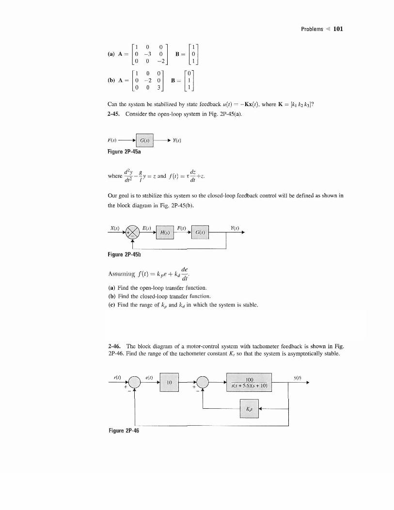
Problems 101
(a) A =
(b) A =
1 0 0
0 - 3 0
0 1 0
- 2 B =
"1" 0 1
1 0 0
0 0 ] - 2 0 0 3
B = ro"
i i
Can the system be stabilized by state feedback «(/) = -Kx(t), where K = [k\ fo^]?
2-45. Consider the open-loop system in Fig. 2P-45(a).
F(s) • G(s) + Y(s)
Figure 2P-45a
d y g dz where - ^ - - -y = z and f{t) = r — +z.
Our goal is to stabilize this system so the closed-loop feedback control will be defined as shown in
the block diagram in Fig. 2P-45(b).
X(s) 7)Eis) > -V * t H(s)
F(s) W G{s)
Y(s) W
Figure 2P-45b
de Assuming / ( f ) = kpe 4- k^ —.
(a) Find the open-loop transfer function.
(b) Find the closed-loop transfer function.
(c) Find the range of kp and kj in which the system is stable.
(d) Suppose T = 1 0 and x = 0.1. If >'(0) = 10 and -j- = 0, then plot the step response of the system
with three different values for kp and kd. Then show that some values are better than others; however, all values must satisfy the Routh-Hurwitz criterion.
2-46. The block diagram of a motor-control system with tachometer feedback is shown in Fig. 2P-46. Find the range of the tachometer constant K, so that the system is asymptotically stable.
rit) ,-^ eit) ^
1 L
10 ,i 1 >
— • 100 s{s + 5.6)(s + 10)
Krs 4
^
y(r) w W
Figure 2P-46

atical Foundation
2-47. The block diagram of a control system is shown in Fig. 2P-47. Find the region in the #-versus-a plane for the system to be asymptotically stable. (Use K as the vertical and a as the horizontal axis.)
"N e(t)
T
s + a s
w.
w K(s + 2)
s2-\
yit)
Figure 2P-47
2-48. The conventional Routh-Hurwitz criterion gives information only on the location of the zeros of a polynomial F(s) with respect to the left half and right half of the .s-plane. Devise a linear transformation s = / ( p , or), where p is a complex variable, so that the Routh-Hurwitz criterion can be applied to determine whether F(s) has zeros to the right of the line s = —a, where or is a positive real number. Apply the transformation to the following characteristic equations to determine how many roots are to the right of the line 5 = - 1 in the s-plane.
(a) F(s) = s2 + 5s + 3 = 0
(b) s* +3s2 + 3s+l=0 (c) F(s) = s3 + As1 + 3s + 10 = 0
(d) s3 +4s2 +45 + 4 = 0
2-49. The payload of a space-shuttle-pointing control system is modeled as a pure mass M. The payload is suspended by magnetic bearings so that no friction is encountered in the control. The attitude of the payload in the y direction is controlled by magnetic actuators located at the base. The total force produced by the magnetic actuators is /(0- The controls of the other degrees of motion are independent and are not considered here. Because there are experiments located on the payload, electric power must be brought to the payload through cables. The linear spring with spring constant Ks is used to model the cable attachment. The dynamic system model for the
Primary Magnet turns
Spindle motor
Magnetic flux
(a)
•o -^»A^ TST^-
+ -O «6 O-
(b)
Figure 2P-49