figure 5.16 see example 5.10. - ees iiest,...
TRANSCRIPT

conductor
Hence,
and
• A
-t—+•
D = 2av nC/m2
SUMMARY • 191
Figure 5.16 See Example 5.10.
E = — = 2 X 10"9 X ~ X 109a, = 36™
= 113.1a, V/m
PRACTICE EXERCISE 5.10
It is found that E = 60ax + 20ay - 30az mV/m at a particular point on the interfacebetween air and a conducting surface. Find D and ps at that point.
Answer: 0.531a* + 0.177ay - 0.265az pC/m2, 0.619 pC/m2.
SUMMARY 1. Materials can be classified roughly as conductors (a ^> 1, sr = 1) and dielectrics(a <sC 1, er > 1) in terms of their electrical properties a and en where a is the con-ductivity and sr is the dielectric constant or relative permittivity.
2. Electric current is the flux of electric current density through a surface; that is,
/ - I 3-dS
3. The resistance of a conductor of uniform cross section is
aS

192 M Electric Fields in Material Space
4. The macroscopic effect of polarization on a given volume of a dielectric material is to"paint" its surface with a bound charge Qh = j>s pps dS and leave within it an accumu-lation of bound charge Qb = fvppv dv where pps = P • an and pp V P.
5. In a dielectric medium, the D and E fields are related as D = sE, where e = eosr is thepermittivity of the medium.
6. The electric susceptibility xe( = er ~ 1) of a dielectric measures the sensitivity of thematerial to an electric field.
7. A dielectric material is linear if D = eE holds, that is, if s is independent of E. It is ho-mogeneous if e is independent of position. It is isotropic if s is a scalar.
8. The principle of charge conservation, the basis of Kirchhoff's current law, is stated inthe continuity equation
dt
9. The relaxation time, Tr = elo, of a material is the time taken by a charge placed in itsinterior to decrease by a factor of e~' — 37 percent.
10. Boundary conditions must be satisfied by an electric field existing in two differentmedia separated by an interface. For a dielectric-dielectric interface
C1 ~p
D^ ~ D2n = ps or Dln = D2r
For a dielectric-conductor interface,
E, = 0 Dn = eEn = ps
because E = 0 inside the conductor.
if ps = 0
REVIEW QUESTIONS
5.1 Which is not an example of convection current?
(a) A moving charged belt
(b) Electronic movement in a vacuum tube
(c) An electron beam in a television tube
(d) Electric current flowing in a copper wire
5.2 When a steady potential difference is applied across the ends of a conducting wire,
(a) All electrons move with a constant velocity.
(b) All electrons move with a constant acceleration.
(c) The random electronic motion will, on the average, be equivalent to a constant veloc-ity of each electron.
(d) The random electronic motion will, on the average, be equivalent to a nonzero con-stant acceleration of each electron.

REVIEW QUESTIONS 193
5.3 The formula R = €/ (oS) is for thin wires.
(a) True
(b) False
(c) Not necessarily
5.4 Sea water has er = 80. Its permittivity is
(a) 81
(b) 79
(c) 5.162 X 10~ l uF/m
(d) 7.074 X 10~10F/m
5.5 Both eo and xe are dimensionless.
(a) True
(b) False
5.6 If V • D = 8 V • E and V - J = < jV-E ina given material, the material is said to be
(a) Linear
(b) Homogeneous
(c) Isotropic
(d) Linear and homogeneous
(e) Linear and isotropic
(f) Isotropic and homogeneous
5.7 The relaxation time of mica (a = 10 mhos/m, er = 6) is
(a) 5 X 10" 1 0 s
(b) 10~6s
(c) 5 hours
(d) 10 hours
(e) 15 hours
5.8 The uniform fields shown in Figure 5.17 are near a dielectric-dielectric boundary but onopposite sides of it. Which configurations are correct? Assume that the boundary is chargefree and that e2 > e^
5.9 Which of the following statements are incorrect?
(a) The conductivities of conductors and insulators vary with temperature and fre-quency.
(b) A conductor is an equipotential body and E is always tangential to the conductor.
(c) Nonpolar molecules have no permanent dipoles.
(d) In a linear dielectric, P varies linearly with E.

194 • Electric Fields in Material Space
© -
(a)
O -
X.
(b) (c)
© . .,
(d) (e)
Figure 5.17 For Review Question 5.8.
(0
PROBLEMS
5.10 The electric conditions (charge and potential) inside and outside an electric screening arecompletely independent of one another.
(a) True
(b) False
Answers: 5.Id, 5.2c, 5.3c, 5.4d, 5.5b, 5.6d, 5.7e, 5.8e, 5.9b, 5.10a.
5.1 In a certain region, J = 3r2 cos 6 ar - r2 sin d as A/m, find the current crossing thesurface defined by 6 = 30°, 0 < 0 < 2TT, 0 < r < 2 m.
500a,5.2 Determine the total current in a wire of radius 1.6 mm if J = A/m2.
P
5.3 The current density in a cylindrical conductor of radius a is
J = l0e-(1~pla}azA/m2
Find the current through the cross section of the conductor.

PROBLEMS • 195
5.4 The charge 10 4e 3( C is removed from a sphere through a wire. Find the current in thewire at t'= 0 and t = 2.5 s.
5.5 (a) Let V = x2y2z in a region (e = 2eo) defined by — 1 < x, y, z < 1. Find the chargedensity pv in the region.
(b) If the charge travels at \(fyay m/s, determine the current crossing surface
0 < x, z < 0.5, y = 1.
5.6 If the ends of a cylindrical bar of carbon (a = 3 X 10⁴) of radius 5 mm and length 8 cmare maintained at a potential difference of 9 V, find: (a) the resistance of the bar, (b) thecurrent through the bar, (c) the power dissipated in the bar.
5.7 The resistance of round long wire of diameter 3 mm is 4.04 fi/km. If a current of 40 Aflows through the wire, find
(a) The conductivity of the wire and identify the material of the wire
(b) The electric current density in the wire
5.8 A coil is made of 150 turns of copper wire wound on a cylindrical core. If the mean radiusof the turns is 6.5 mm and the diameter of the wire is 0.4 mm, calculate the resistance ofthe coil.
5.9 A composite conductor 10 m long consists of an inner core of steel of radius 1.5 cm andan outer sheath of copper whose thickness is 0.5 cm.
(a) Determine the resistance of the conductor.
(b) If the total current in the conductor is 60 A, what current flows in each metal?
(c) Find the resistance of a solid copper conductor of the same length and cross-sectionalareas as the sheath. Take the resistivities of copper and steel as 1.77 X 10"8 and11.8 X 10"8 0 • m, respectively.
5.10 A hollow cylinder of length 2 m has its cross section as shown in Figure 5.18. If the cylin-der is made of carbon (a = 105 mhos/m), determine the resistance between the ends ofthe cylinder. Take a — 3 cm, b = 5 cm.
5.11 At a particular temperature and pressure, a helium gas contains 5 X 1025 atoms/m3. If a10-kV/m field applied to the gas causes an average electron cloud shift of 10" '8 m, findthe dielectric constant of helium.
Figure 5.18 For Problems 5.10 and 5.15.

196 • Electric Fields in Material Space
5.12 A dielectric material contains 2 X 10¹⁹ polar molecules/m3, each of dipole moment1.8 X 10~27C/m. Assuming that all the dipoles are aligned in the direction of the electricfield E = 105 ax V/m, find P and sr.
5.13 In a slab of dielectric material for which e = 2.48O and V = 300z2 V, find: (a) D and pv,(b)Pandppv.
5.14 For x < 0, P = 5 sin (ay) ax, where a is a constant. Find pps and ppv.
5.15 Consider Figure 5.18 as a spherical dielectric shell so that 8 = eoer for a < r < b ande = eo for 0 < r < a. If a charge Q is placed at the center of the shell, find
(a) P for a < r < b
(b) ppvfora <r<b
(c) pps at r = a and r = b
5.16 Two point charges when located in free space exert a force of 4.5 /uN on each other. Whenthe space between them is filled with a dielectric material, the force changes to 2 /xN. Findthe dielectric constant of the material and identify the material.
5.17 A conducting sphere of radius 10 cm is centered at the origin and embedded in a dielectricmaterial with e = 2.5eo. If the sphere carries a surface charge of 4 nC/m2, find E at( — 3 cm, 4 cm, 12 cm).
5.18 At the center of a hollow dielectric sphere (e = eoer) is placed a point charge Q. If thesphere has inner radius a and outer radius b, calculate D, E, and P.
5.19 A sphere of radius a and dielectric constant er has a uniform charge density of po.
(a) At the center of the sphere, show that
(b) Find the potential at the surface of the sphere.
5.20 For static (time-independent) fields, which of the following current densities are possible?
(a) J = 2x3yax 4x2z\ - 6x2yzaz
(b) J = xyax + y(z + l)ay
(c) J = — ap + z cos 4> az
5.21 For an anisotropic medium
Obtain D for: (a) E = 10a., + 10a,, V/m, (b) E = 10a^ + 203 , - 30az V/m.
VDy
Dz
= so
411
141
114
Ex
Ey
Ez

PROBLEMS 8 197
100 . . 25.22 If J = — Y ap A/m , find: (a) the rate of increase in the volume charge density, (b) theP
t o t a l c u r r e n t p a s s i n g t h r o u g h s u r f a c e d e f i n e d b y p = 2 , 0 < z < \ , 0 < <f> < 2 i r .
5 e - io 4 »5.23 Given that J = ar A/m2, at t = 0.1 ms, find: (a) the amount of current passing
rsurface r = 2 m, (b) the charge density pv on that surface.
5.24 Determine the relaxation time for each of the following medium:
(a) Hard rubber (a = 10~15 S/m, e = 3.1eo)(b) Mica (ff = 10"15 S/m, e = 6eo)(c) Distilled water (a = 10~4 S/m, e = 80eo)
5.25 The excess charge in a certain medium decreases to one-third of its initial value in 20 /xs.(a) If the conductivity of the medium is 10 4 S/m, what is the dielectric constant of themedium? (b) What is the relaxation time? (c) After 30 [is, what fraction of the charge willremain?
5.26 Lightning strikes a dielectric sphere of radius 20 mm for which er = 2.5, a =5 X 10~6 mhos/m and deposits uniformly a charge of 10 /JLC. Determine the initialcharge density and the charge density 2 ps later.
5.27 Region 1 (z < 0) contains a dielectric for which er = 2.5, while region 2 (z > 0) is char-acterized by er = 4. Let E, = -30a^ + 50a,, + 70az V/m and find: (a) D2, (b) P2,(c) the angle between Ei and the normal to the surface.
5.28 Given that E, = 10a^ - 6a,, + 12a, V/m in Figure 5.19, find: (a) Pu (b) E2 and theangle E2 makes with the y-axis, (c) the energy density in each region.
5.29 Two homogeneous dielectric regions 1 (p < 4 cm) and 2 (p > 4 cm) have dielectricconstants 3.5 and 1.5, respectively. If D2 = 12ap - 6a0 + 9az nC/m2, calculate: (a) Eiand D,, (b) P2 and ppv2, (c) the energy density for each region.
5.30 A conducting sphere of radius a is half-embedded in a liquid dielectric medium of per-mittivity s, as in Figure 5.20. The region above the liquid is a gas of permittivity e2. If thetotal free charge on the sphere is Q, determine the electric field intensity everywhere.
*5.31 Two parallel sheets of glass (er = 8.5) mounted vertically are separated by a uniform airgap between their inner surface. The sheets, properly sealed, are immersed in oil(er = 3.0) as shown in Figure 5.21. A uniform electric field of strength 2000 V/m in thehorizontal direction exists in the oil. Calculate the magnitude and direction of the electricfield in the glass and in the enclosed air gap when (a) the field is normal to the glass sur-faces, and (b) the field in the oil makes an angle of 75° with a normal to the glass surfaces.Ignore edge effects.
5.32 (a) Given that E = 15a^ - 8az V/m at a point on a conductor surface, what is thesurface charge density at that point? Assume e = e0.
(b) Region y > 2 is occupied by a conductor. If the surface charge on the conductor is— 20 nC/m2, find D just outside the conductor.

198 11 Electric Fields in Material Space
© e, = 3E0
Ei = 4.5B
Figure 5.19 For Problem 5.28.
Figure 5.20 For Problem 5.30.
glass Figure 5.21 For Problem 5.31.
oil oil
5.33 A silver-coated sphere of radius 5 cm carries a total charge of 12 nC uniformly distributedon its surface in free space. Calculate (a) |D| on the surface of the sphere, (b) D externalto the sphere, and (c) the total energy stored in the field.

Chapter 6
ELECTROSTATIC BOUNDARY-VALUE PROBLEMS
Our schools had better get on with what is their overwhelmingly most importanttask: teaching their charges to express themselves clearly and with precision inboth speech and writing; in other words, leading them toward mastery of theirown language. Failing that, all their instruction in mathematics and science is awaste of time.
—JOSEPH WEIZENBAUM, M.I.T.
b.1 INTRODUCTION
The procedure for determining the electric field E in the preceding chapters has generallybeen using either Coulomb's law or Gauss's law when the charge distribution is known, orusing E = — W when the potential V is known throughout the region. In most practicalsituations, however, neither the charge distribution nor the potential distribution is known.
In this chapter, we shall consider practical electrostatic problems where only electro-static conditions (charge and potential) at some boundaries are known and it is desired tofind E and V throughout the region. Such problems are usually tackled using Poisson's1 orLaplace's2 equation or the method of images, and they are usually referred to as boundary-value problems. The concepts of resistance and capacitance will be covered. We shall useLaplace's equation in deriving the resistance of an object and the capacitance of a capaci-tor. Example 6.5 should be given special attention because we will refer to it often in theremaining part of the text.
.2 POISSON'S AND LAPLACE'S EQUATIONS
Poisson's and Laplace's equations are easily derived from Gauss's law (for a linear mater-ial medium)
V • D = V • eE = pv (6.1)
'After Simeon Denis Poisson (1781-1840), a French mathematical physicist.2After Pierre Simon de Laplace (1749-1829), a French astronomer and mathematician.
199

200 Electrostatic Boundary-Value Problems
and
E = -VV
Substituting eq. (6.2) into eq. (6.1) gives
V-(-eVV) = pv
for an inhomogeneous medium. For a homogeneous medium, eq. (6.3) becomes
V2y = - ^
(6.2)
(6.3)
(6.4)
This is known as Poisson's equation. A special case of this equation occurs when pv = 0(i.e., for a charge-free region). Equation (6.4) then becomes
V2V= 0 (6.5)
which is known as Laplace's equation. Note that in taking s out of the left-hand side ofeq. (6.3) to obtain eq. (6.4), we have assumed that e is constant throughout the region inwhich V is defined; for an inhomogeneous region, e is not constant and eq. (6.4) does notfollow eq. (6.3). Equation (6.3) is Poisson's equation for an inhomogeneous medium; itbecomes Laplace's equation for an inhomogeneous medium when pv = 0.
Recall that the Laplacian operator V2 was derived in Section 3.8. Thus Laplace's equa-tion in Cartesian, cylindrical, or spherical coordinates respectively is given by
(6.6)
(6.7)
(6.8)
depending on whether the potential is V(x, y, z), V(p, 4>, z), or V(r, 6, 4>). Poisson's equationin those coordinate systems may be obtained by simply replacing zero on the right-handside of eqs. (6.6), (6.7), and (6.8) with —pv/e.
Laplace's equation is of primary importance in solving electrostatic problems involv-ing a set of conductors maintained at different potentials. Examples of such problemsinclude capacitors and vacuum tube diodes. Laplace's and Poisson's equations are not onlyuseful in solving electrostatic field problem; they are used in various other field problems.
1
r2
d f 2
1
P
3rJ
3
da
11
( 3\
-> V dp
1
r2sin
+
A
32V
8y2
1
P
a /36 \
d2V
d2V2 30 2 +
aysin u
36,
= 0
a2vaz2
) ,i ' r2
0
1
sin2 6
32V~
3<j>20
6.3 UNIQUENESS THEOREM 201
For example, V would be interpreted as magnetic potential in magnetostatics, as tempera-ture in heat conduction, as stress function in fluid flow, and as pressure head in seepage.
6.3 UNIQUENESS THEOREM
Since there are several methods (analytical, graphical, numerical, experimental, etc.) ofsolving a given problem, we may wonder whether solving Laplace's equation in differentways gives different solutions. Therefore, before we begin to solve Laplace's equation, weshould answer this question: If a solution of Laplace's equation satisfies a given set ofboundary conditions, is this the only possible solution? The answer is yes: there is only onesolution. We say that the solution is unique. Thus any solution of Laplace's equation whichsatisfies the same boundary conditions must be the only solution regardless of the methodused. This is known as the uniqueness theorem. The theorem applies to any solution ofPoisson's or Laplace's equation in a given region or closed surface.
The theorem is proved by contradiction. We assume that there are two solutions V\ andV2 of Laplace's equation both of which satisfy the prescribed boundary conditions. Thus
V 2 ^ = 0,
v, = v7
V2V2 = 0
on the boundary
We consider their difference
vd = v2 - v,which obeys
v2yrf = v2y2 - v2y, = o
Vd = 0 on the boundary
according to eq. (6.9). From the divergence theorem.
V • A dv = I A • dS^s
We let A = Vd VVd and use a vector identity
V • A = V • (VdWd) = VdV2Vd + Wd • VVd
But V2Vd = 0 according to eq. (6.11), so
V • A = VVd • VVd
Substituting eq. (6.13) into eq. (6.12) gives
VVd- VVddv= <j) VdWd-dS
(6.9a)
(6.9b)
(6.10)
(6.11a)
(6.11b)
(6.12)
(6.13)
(6.14)
From eqs. (6.9) and (6.11), it is evident that the right-hand side of eq. (6.14) vanishes.

202 Electrostatic Boundary-Value Problems
Hence:
VVJ2dv = 0
Since the integration is always positive.
or
W r f = 0
Vd — V2 — V\ = constant everywhere in v
(6.15a)
(6.15b)
But eq. (6.15) must be consistent with eq. (6.9b). Hence, Vd = 0 or V, = V2 everywhere,showing that Vx and V2 cannot be different solutions of the same problem.
This is the uniqueness theorem: If a solution lo Laplace's equation can be foundliii.it salisties the boundary conditions, ihcn the solution is unique.
Similar steps can be taken to show that the theorem applies to Poisson's equation and toprove the theorem for the case where the electric field (potential gradient) is specified onthe boundary.
Before we begin to solve boundary-value problems, we should bear in mind the threethings that uniquely describe a problem:
1. The appropriate differential equation (Laplace's or Poisson's equation in thischapter)
2. The solution region3. The prescribed boundary conditions
A problem does not have a unique solution and cannot be solved completely if any of thethree items is missing.
6.4 GENERAL PROCEDURE FOR SOLVING POISSON'SOR LAPLACE'S EQUATION
The following general procedure may be taken in solving a given boundary-value probleminvolving Poisson's or Laplace's equation:
1. Solve Laplace's (if pv = 0) or Poisson's (if pv =£ 0) equation using either (a) directintegration when V is a function of one variable, or (b) separation of variables if Vis a function of more than one variable. The solution at this point is not unique butexpressed in terms of unknown integration constants to be determined.
2. Apply the boundary conditions to determine a unique solution for V. Imposing thegiven boundary conditions makes the solution unique.
3. Having obtained V, find E using E = - VV and D from D = eE.

6.4 GENERAL PROCEDURE FOR SOLVING POISSON'S OR LAPLACE'S EQUATION 203
4. If desired, find the charge Q induced on a conductor using Q = J ps dS whereps — Dn and Dn is the component of D normal to the conductor. If necessary, thecapacitance between two conductors can be found using C = Q/V.
Solving Laplace's (or Poisson's) equation, as in step 1, is not always as complicated asit may seem. In some cases, the solution may be obtained by mere inspection of theproblem. Also a solution may be checked by going backward and finding out if it satisfiesboth Laplace's (or Poisson's) equation and the prescribed boundary conditions.
EXAMPLE 6.1Current-carrying components in high-voltage power equipment must be cooled to carryaway the heat caused by ohmic losses. A means of pumping is based on the force transmit-ted to the cooling fluid by charges in an electric field. The electrohydrodynamic (EHD)pumping is modeled in Figure 6.1. The region between the electrodes contains a uniformcharge p0, which is generated at the left electrode and collected at the right electrode. Cal-culate the pressure of the pump if po = 25 mC/m3 and Vo = 22 kV.
Solution:
Since p,, # 0, we apply Poisson's equation
V2V = - ^8
The boundary conditions V(z = 0) = Vo and V(z = d) = 0 show that V depends only on z(there is no p or <j> dependence). Hence
d2v -dz2
Integrating once gives
Integrating again yields
dV _ ~dz
V = -— + Az + B2e
AreaS
Figure 6.1 An electrohydrodynamic pump; forExample 6.1.

204 Electrostatic Boundary-Value Problems
where A and B are integration constants to be determined by applying the boundary condi-tions. When z = 0, V = Vo,
Vo = - 0 + 0 + B -> B = Vo
When z = d, V = 0,
2e
or
A =2e d
The electric field is given by
The net force is
F = | pvE dv = p0 | dS \ Edz
F = PoSVoaz
The force per unit area or pressure is
p =- = poVo = 25 X 1(T3 X 22 X 103 = 550N/m2
PRACTICE EXERCISE 6.1
In a one-dimensional device, the charge density is given by pv =x = 0 and V = 0 at x = a, find V and E.
. If E = 0 at
Answer: - ^ (a3 - A ^tea 2ae
EXAMPLE 6.2The xerographic copying machine is an important application of electrostatics. The surfaceof the photoconductor is initially charged uniformly as in Figure 6.2(a). When light fromthe document to be copied is focused on the photoconductor, the charges on the lower

6.4 GENERAL PROCEDURE FOR SOLVING POISSON'S OR LAPLACE'S EQUATION • 205
photoconductor
light
:'.:'.T- '. recombination
(a)
I- T - i - ^ •> t r - - + 1- J- - + » + - - -
(b)
Figure 6.2 For Example 6.2.
surface combine with those on the upper surface to neutralize each other. The image is de-veloped by pouring a charged black powder over the surface of the photoconductor. Theelectric field attracts the charged powder, which is later transferred to paper and melted toform a permanent image. We want to determine the electric field below and above thesurface of the photoconductor.
Solution:
Consider the modeled version of Figure 6.2(a) as in Figure 6.2(b). Since pv = 0 in thiscase, we apply Laplace's equation. Also the potential depends only on x. Thus
= 0dx2
Integrating twice gives
V = Ax + B
Let the potentials above and below be Vx and V2, respectively.
V1 = Axx + Bu x > a
V2 = A2x + B2, x<a
(6.2.1a)
(6.2.1b)

206 Electrostatic Boundary-Value Problems
The boundary conditions at the grounded electrodes are
V,(* = d) = 0
V2(x = 0) = 0
At the surface of the photoconductor,
Vx(x = a) = V2(x = a)
Dln ~ D2n = ps
(6.2.2.a)
(6.2.2b)
(6.2.3a)
(6.2.3b)
We use the four conditions in eqs. (6.2.2) and (6.2.3) to determine the four unknown con-stants Ai,A2, B1; andB2. From eqs. (6.2.1) and 6.2.2),
0 = A,d + B, -> B, = -Axd
0 = 0 + B2-^B2 = 0
From eqs. (6.2.1) and (6.2.3a),
A{a + B, = A2a
To apply eq. (6.2.3b), recall that D = eE = - e W so that
Ps = Din - D2n = £,£,„ - e2E2n = - e , —— + e2——ax ax
or
Ps = ~eiAi + e2A2
Solving for Aj and A2 in eqs. (6.2.4) to (6.2.6), we obtain
E, = -A,ax =
S |s7 d B7
e, a s.
7 = -A7a r =I , , s2 d s2
(6.2.4a)
(6.2.4b)
(6.2.5)
(6.2.6)
PRACTICE EXERCISE 6.2
For the model of Figure 6.2(b), if ps — 0 and the upper electrode is maintained at Vo
while the lower electrode is grounded, show that
d — a -\ a
E,-Voax \.
£2 A £ 2a a

EXAMPLE 6.3
6.4 GENERAL PROCEDURE FOR SOLVING POISSON'S OR LAPLACE'S EQUATION • 207
Semiinfinite conducting planes <j> = 0 and <f> = TT/6 are separated by an infinitesimal insu-lating gap as in Figure 6.3. If V(<£ = 0) = 0 and V(<t> = TT/6) = 100 V, calculate V and Ein the region between the planes.
Solution:
As V depends only on </>, Laplace's equation in cylindrical coordinates becomes
Since p = 0 is excluded due to the insulating gap, we can multiply by p2 to obtain
d2V
d<p2 = 0
which is integrated twice to give
V = Acf> + B
We apply the boundary conditions to determine constants A and B. When 4> — 0, V = 0,
0 = 0 + B^B = 0
W h e n 4> = <f>o, V = Vo,
'-, Hence:
gap
Figure 6.3 Potential V(<j>) due to semi-infinite conducting planes.
— y

208 B Electrostatic Boundary-Value Problems
and
Substituting Vo = 100 and <j>0 = TT/6 gives
600V = and
Check: = 0, V(</> = 0) = 0, V(</> = TT/6) = 100.
PRACTICE EXERCISE 6.3
Two conducting plates of size 1 X 5 m are inclined at 45° to each other with a gap ofwidth 4 mm separating them as shown in Figure 6.4. Determine an approximatevalue of the charge per plate if the plates are maintained at a potential difference of50 V. Assume that the medium between them has er = 1.5.
Answer: 22.2 nC.
EXAMPLE 6.4Two conducting cones (6 = TT/10 and 6 = x/6) of infinite extent are separated by an infin-itesimal gap at r = 0. If V(6 = TT/10) = 0 and V(6 = TT/6) = 50 V, find V and E betweenthe cones.
Solution:
Consider the coaxial cone of Figure 6.5, where the gap serves as an insulator between thetwo conducting cones. V depends only on 6, so Laplace's equation in spherical coordinatesbecomes
r2sin 6
gap of width 4 mm
Figure 6.4 For Practice Exercise 6.3.
1 m

6.4 GENERAL PROCEDURE FOR SOLVING POISSON'S OR LAPLACE'S EQUATION • 209
Figure 6.5 Potential V(4>) due to conducting cones.
Since r = 0 and 0 = 0, it are excluded, we can multiply by r2sin 0 to get
Integrating once gives
or
dV- = A
dV A
dd sin 0
Integrating this results in
d9V = A \ - F T = A
= A
= A
dd
sin 9 " J 2 cos 0/2 sin 9/21/2 sec2 (9/2 dd
tan 0/2J(tan 0/2)
tan 9/2= A In (tan 0/2) + B
We now apply the boundary conditions to determine the integration constants A and B.
V{9 = 00 = 0 -> 0 = A In (tan 0,/2) + B
or
B = -A In (tan 0,/2)

210 M Electrostatic Boundary-Value Problems
Hence
Also
or
Thus
V = A Intan 0/2tan 0,/2
V{9 = 62) = Vo -» Vo = A Intan 02/2tan 0,/2
A =
Intan 02/2
V =
tan 0/2
tan 0,/2
Intan 02/2tan 0,/2
r sin 0
r sin 0 In
Taking 0, = TT/10, 02 = ir/6, and Vo = 50 gives
tan 02/2
tan 0,/2
50 In
V =
tan 0/2 jLtan7r/2oJ
Intan TT/12
tan TT/20
tan 0/2]
and
E =r sin 0
Check: V2V = 0, V(9 = TT/10) = 0, V(0 = TT/6) = Vo.

6.4 GENERAL PROCEDURE FOR SOLVING POISSON'S OR LAPLACE'S EQUATION 211
50 V
gap
For Practice Exercise 6.4.
1
PRACTICE EXERCISE 6.4
A large conducting cone (d = 45°) is placed on a conducting plane with a tiny gapseparating it from the plane as shown in Figure 6.6. If the cone is connected to a50-V source, find V and E at ( - 3 , 4, 2).
Answer: 22.13 V, 11.36 a» V/m.
(a) Determine the potential function for the region inside the rectangular trough of infinitelength whose cross section is shown in Figure 6.7.
(b) For Vo = 100 V and b = 2a, find the potential at x = a/2, y = 3a/4.
Solution:
(a) The potential V in this case depends on x and y. Laplace's equation becomes
v2y =dx- dr
T = 0 (6.5.1)
Potential V(x, y) due to a con-ducting rectangular trough.

Electrostatic Boundary-Value Problems
We have to solve this equation subject to the following boundary conditions:
V(x = 0, 0 < y < a) = 0 (6.5.2a)
V(x = b, 0 < y < a) = 0 (6.5.2b)
V(0 < A: < b, y = 0) = 0 (6.5.2c)
V{0<x<b,y = a) = Vo (6.5.2d)
We solve eq. (6.5.1) by the method of separation of variables; that is, we seek a productsolution of V. Let
V(x, y) = X(x) Y(y) (6.5.3)
when X is a function of x only and y is a function of >• only. Substituting eq. (6.5.3) intoeq. (6.5.1) yields
X"Y + Y"X = 0
Dividing through by XY and separating X from Y gives
X" Y"-J = y (6.5.4a)
Since the left-hand side of this equation is a function of x only and the right-hand side is afunction of y only, for the equality to hold, both sides must be equal to a constant X; that is
rY
(6.5.4b)
The constant X is known as the separation constant. From eq. (6.5.4b), we obtain
X" + XX = 0 (6.5.5a)
and
Y" - \Y = 0 (6.5.5b)
Thus the variables have been separated at this point and we refer to eq. (6.5.5) as separatedequations. We can solve for X(x) and Y(y) separately and then substitute our solutions intoeq. (6.5.3). To do this requires that the boundary conditions in eq. (6.5.2) be separated, ifpossible. We separate them as follows:
V(0, y) = X(0)Y(y) = 0 -> X(0) = 0
V(b, y) = X(b)Y(y) = 0 -* X(b) = 0
V(x, 0) = X(x)Y(0) = 0 -> Y(0) = 0
V(x, a) = X(0)Y(a) = Vo (inseparable)
(6.5.6a)
(6.5.6b)
(6.5.6c)
(6.5.6d)
To solve for X(;c) and Y(y) in eq. (6.5.5), we impose the boundary conditions in eq. (6.5.6).We consider possible values of X that will satisfy both the separated equations in eq. (6.5.5)and the conditions in eq. (6.5.6).

6.4 GENERAL PROCEDURE FOR SOLVING POISSON'S OR LAPLACE'S EQUATION 213
CASE A.
If X = 0, then eq. (6.5.5a) becomes
X" = 0 ordx2
(6.5.7)
which, upon integrating twice, yields
X = Ax + B
The boundary conditions in eqs. (6.5.6a) and (6.5.6b) imply that
XQt = 0) = 0 ^ 0 = 0 + fi or 5 = 0
and
X(x = b) = 0-^0 = A- b + 0 or A = 0
because b # 0. Hence our solution for X in eq. (6.5.7) becomes
X(x) = 0
which makes V = 0 in eq. (6.5.3). Thus we regard X(x) = 0 as a trivial solution and weconclude that A # 0.
CASE B.
If X < 0, say X = — or, then eq. (6.5.5a) becomes
X" - aX = 0 or (D2 - a2)X = 0
where D = —dx
that is,
DX = ±aX
showing that we have two possible solutions corresponding to the plus and minus signs.For the plus sign, eq. (6.5.8) becomes
dX dX— = aX or — = a dxdx X
(6.5.S
= a dx or In X = ax + In A,
where In /i, is a constant of integration. Thus
X = Axeax (6.5.9a)

:14 : ectrostatic Boundary-Value Problems
Similarly, for the minus sign, solving eq. (6.5.8) gives
X = A2e~ax (6.5.9b)
The total solution consists of what we have in eqs. (6.5.9a) and (6.5.9b); that is,
X(x) = A,eax + A2e~ax (6.5.10)
Since cosh ax = (eax + <Tajr)/2 and sinh ax = (eax ~ e~ax)l2 or eax = cosh ax +sinh ax and e ax = cosh ax — sinh ax, eq. (6.5.10) can be written as
X(x) = B] cosh ax + B2 sinh ax (6.5.11)
where Bx = A, + A2 and B2 = A, — A2. In view of the given boundary conditions, weprefer eq. (6.5.11) to eq. (6.5.10) as the solution. Again, eqs. (6.5.6a) and (6.5.6b) requirethat
X(x = 0) = 0 ^ 0 = S, • (1) + B2 • (0) or 5, = 0
and
X(x = 6) = , sinh ab
Since a ¥= 0 and & # 0, sinh a£> cannot be zero. This is due to the fact that sinh x = 0 ifand only if x = 0 as shown in Figure 6.8. Hence B2 = 0 and
X(x) = 0
This is also a trivial solution and we conclude that X cannot be less than zero.
CASE C.
If X > 0, say X = /32, then eq. (6.5.5a) becomes
X" + (32X = 0
cosh x~
2 - 1
- sinh x
Sketch of cosh x and sinh xshowing that sinh x = 0 if and only if.« = 0.
6.4 GENERAL PROCEDURE FOR SOLVING POISSON'S OR LAPLACE'S EQUATION 215
that is,
(D1 + (32)X = 0 or DX = ±j(SX (6.5.12)
where / = V — 1. From eqs. (6.5.8) and (6.5.12), we notice that the difference betweenCases 2 and 3 is replacing a by/'j3. By taking the same procedure as in Case 2, we obtainthe solution as
X(x) = t > / f a + e V - " i l (6.5.13a)
Since eliix = cos (3x + j sin fix and e~-itix = cos (3x — j sin /3.v, eq. (6.5.13a) can be written
X(.x) = ga cos /3.v + 'i sin fix
where g() = Co + C, and ^, = Co - ,/C,.In view of the given boundary conditions, we prefer to use eq. (6.5.13b). Imposing the
conditions in eqs. (6.5.6a) and (6.5.6b) yields
X(x = 0) = 0 -> 0 = #o • (1) + 0
and
X(x = b) = 0 - > 0 = 0 + £, sin/3/?
Suppose #, ¥= 0 (otherwise we get a trivial solution), then
sin (3b = 0 = sin nir
& = —. H = 1,2, 3,4, . . .
(6.5.13b)
J?., = 0
(6.5.14)
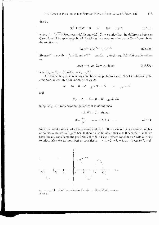
Note that, unlike sinh .v, which is zero only when ,v = 0. sin .v is zero at an infinite numberof points as shown in Figure 6.9. It should also be noted that n + 0 because (3 + 0; wehave already considered the possibility /3 = 0 in Case 1 where we ended up with a trivialsolution. Also we do not need to consider n = — 1, —2, —3. —4, . . . because X = j32
^ 1-2 ix 3 jr i
( :-;isf, c..v Sketch of sin x showing that sin x = 0 at infinite n u m b e r
of points .

216 Electrostatic Boundary-Value Problems
would remain the same for positive and negative values of n. Thus for a given n,eq. (6.5.13b) becomes
Xn(x) = gn sin —
Having found X(x) and
(6.5.15)
(6.5.16)
we solve eq. (6.5.5b) which is now
Y" - (32Y = 0
The solution to this is similar to eq. (6.5.11) obtained in Case 2 that is,
Y(y) = h0 cosh /3y + hx sinh j3y
The boundary condition in eq. (6.5.6c) implies that
Y(y = 0) = 0 - > 0 = V ( l ) + 0 or ho = 0
Hence our solution for Y(y) becomes
Yn(y) = K sinh —— (6.5.17)
Substituting eqs. (6.5.15) and (6.5.17), which are the solutions to the separated equationsin eq. (6.5.5), into the product solution in eq. (6.5.3) gives
Vn(x, y) = gnhn sin —— sinh ——b b
This shows that there are many possible solutions Vb V2, V3, V4, and so on, for n =1, 2, 3, 4, and so on.
By the superposition theorem, if V,, V2, V3, . . . ,Vn are solutions of Laplace's equa-tion, the linear combination
v = c2v2 + c3v3 +• cnvn
(where cu c2, c 3 . . . , cn are constants) is also a solution of Laplace's equation. Thus thesolution to eq. (6.5.1) is
V(x, y) = 2J cn sin - — sinh ——«=i b b
(6.5.18)
where cn = gnhn are the coefficients to be determined from the boundary condition ineq. (6.5.6d). Imposing this condition gives
V(x, y = a) = Vo = 2J cn sin —— smh ——« = i b b
(6.5.19)

6.4 GENERAL PROCEDURE FOR SOLVING POISSON'S OR LAPLACE'S EQUATION • 217
which is a Fourier series expansion of Vo. Multiplying both sides of eq. (6.5.19) bysin m-KxIb and integrating over 0 < x < b gives
mirx --, mra mirx mrxVnSin dx = >, cn S l n h sin sin dx
Jo b n-e, b }0 b b
By the orthogonality property of the sine or cosine function (see Appendix A.9).
'0, m + n
(6.5.20)
sin mx sin nx dx =TT/2, m = n
Incorporating this property in eq. (6.5.20) means that all terms on the right-hand side ofeq. (6.5.20) will vanish except one term in which m = n. Thus eq. (6.5.20) reduces to
b rbmrx mra , mrx
Vosin dx = cn sinh | sin —r~ dx
or
that is,
o o
n-wx— cos ——n-K b
= cn sinh mra 1 — cos
Vob mra b(1 — cos mr) = cn sinh • —
n-K b 2
. mra 2VOcn smh = (I — cos rnr)
b nic
b Jdx
^ , n = 1,3,5,-
[ 0, n = 2 , 4 , 6 , . . .
cn = \ mr sinh
0,
mran = odd
n = even
Substituting this into eq. (6.5.18) gives the complete solution as
V(x,y) =
mrx nirysin sinh
b b
n sinhn-K a
(6.5.21)
(6.5.22)
Check: V2V = 0, V(x = 0, y) = 0 = V(x = b, y) = V(x, y, = 0), V(x, y = a) = Vo. Thesolution in eq. (6.5.22) should not be a surprise; it can be guessed by mere observation ofthe potential system in Figure 6.7. From this figure, we notice that along x, V varies from

218 Electrostatic Boundary-Value Problems
0 (at x = 0) to 0 (at x = b) and only a sine function can satisfy this requirement. Similarly,along y, V varies from 0 (at y = 0) to Vo (at y = a) and only a hyperbolic sine function cansatisfy this. Thus we should expect the solution as in eq. (6.5.22).
To determine the potential for each point (x, y) in the trough, we take the first fewterms of the convergent infinite series in eq. (6.5.22). Taking four or five terms may be suf-ficient,(b) For x = a/2 and y = 3a/4, where b = 2a, we have
2' 4
4V2
n= 1,3,5
sin «7r/4 sinh 3«TT/8
n sinh rnr/2sin ir/4 sinh 3TT/8 sin 3TT/4 sinh 9TT/8
3 sinh 3TT/2T [ sinh x/2sin 5x/4 sinh 15ir/4
5 sinh 5TT/4
4V= —£(0.4517 + 0.0725 - 0.01985 - 0.00645 + 0.00229 + • • •)
IT
= 0.6374Vo
It is instructive to consider a special case when A = b = Ira and Vo = 100 V. The poten-tials at some specific points are calculated using eq. (6.5.22) and the result is displayed inFigure 6.10(a). The corresponding flux lines and equipotential lines are shown in Figure6.10(b). A simple Matlab program based on eq. (6.5.22) is displayed in Figure 6.11. Thisself-explanatory program can be used to calculate V(x, y) at any point within the trough. InFigure 6.11, V(x = b/A, y = 3a/4) is typically calculated and found to be 43.2 volts.
1.0
100 VEquipotential line
Flux line
43.2 54.0 43.2
18.2 25.0 18.2
6.80 9.54 6.80
(a)
1.0 0
Figure 6.10 For Example 6.5: (a) V(x, y) calculated at some points, (b) sketch of flux linesand equipotential lines.

6.4 GENERAL PROCEDURE FOR SOLVING POISSON'S OR LAPLACE'S EQUATION 219
% SOLUTION OF LAPLACE'S EQUATION%
% THIS PROGRAM SOLVES THE TWO-DIMENSIONAL% BOUNDARY-VALUE PROBLEM DESCRIBED IN FIG. 6.7% a AND b ARE THE DIMENSIONS OF THE TROUGH% x AND y ARE THE COORDINATES OF THE POINT% OF INTEREST
P = [ ] ;Vo = 100.0;a = 1.0;b = a;x = b/4;y= 3.*a/4.;c = 4.*Vo/pisum = 0.0;for k=l:10
n = 2*k - 1al = sin(n*pi*x/b);a2 = sinh(n*pi*y/b);a3 = n*sinh(n*pi*a/b);sum = sum + c*al*a2/a3;P = [n, sum]
enddiary test.outPdiary off
Figure 6.11 Matlab program for Example 6.5.
PRACTICE EXERCISE 6.5
For the problem in Example 6.5, take Vo = 100 V, b = 2a = 2 m, find V and E at
(a) (x,y) = (a,a/2)
(b) (x,y) = (3a/2,a/4)
Answer: (a) 44.51 V, -99.25 ay V/m, (b) 16.5 V, 20.6 ax - 70.34 ay V/m.
EXAMPLE 6.6In the last example, find the potential distribution if Vo is not constant but
(a) Vo = 10 s in 3irx/b, y = a, Q<x<b
( b ) VQ = 2 sin y + — sin - y , y = a,0<x<b
220 M Electrostatic Boundary-Value Problems
Solution:
(a) In the last example, every step before eq. (6.5.19) remains the same; that is, the solu-tion is of the form
^ , nirx niryV(x, y) = 2J cn sin —— sinh ——
t^x b b
as per eq. (6.5.18). But instead of eq. (6.5.19), we now have
V(y = a) = Vo = 10 sin —— = X cn sin —— sinhb n=i b b
By equating the coefficients of the sine terms on both sides, we obtain
For n = 3,
10 = c3 sinh3ira
or
10
sinh3ira
Thus the solution in eq. (6.6.1) becomes
V(x,y) = 10 sin3TTX
sinh
sinh
(b) Similarly, instead of eq. (6.5.19), we have
Vo = V(y = a)
or
5-KX•KX 12 sin 1 sinh
b 10 b
Equating the coefficient of the sine terms:
«7TXcn sinh sinh
cn = 0, n * 1,5
(6.6.1)
6.4 GENERAL PROCEDURE FOR SOLVING POISSON'S OR LAPLACE'S EQUATION
Forn = 1,
2 = cx sinh — orb
221
For n = 5,
Hence,
sinh-ira
1 5ira- = c5sinh — or c5 =
10 sinh5ira
V(x,y) =
. irx . Try 5irx 5iry2 sm — sinh — sin sinh
b b b b+
sinh —b
10 sinh5ira
PRACTICE EXERCISE 6.6
In Example 6.5, suppose everything remains the same except that Vo is replaced by
Vo sin ——, 0 < x < b, y = a. Find V(JC, y).
Answer:Vn sin sinh
sinh7ra
EXAMPLE 6.7 Obtain the separated differential equations for potential distribution V(p, </>, z) in a charge-free region.
Solution:
This example, like Example 6.5, further illustrates the method of separation of variables.Since the region is free of charge, we need to solve Laplace's equation in cylindrical coor-dinates; that is,
a / dv\ 1P — I + —
d2V d2V
We let
P dp \ dp) p2 d(j>-
V(p, 4>, z) = R{P) Z(Z)
(6.7.1)
(6.7.2)

222 H Electrostatic Boundary-Value Problems
where R, <P, and Z are, respectively, functions of p, (j>, and z. Substituting eq. (6.7.2) into
eq. (6.7.1) gives
*?p dp\dp
We divide through by R<PZ to obtain
p2 d<t>2 T = 0
\_±(pdR\ 1 d2t>pR dp\ dp ) P
2<P d<t>
dz
1 d2Z
Z dz2
(6.7.3)
(6.7.4)
The right-hand side of this equation is solely a function of z whereas the left-hand sidedoes not depend on z. For the two sides to be equal, they must be constant; that is,
J_d_(pdR\ +J_d*±pR dp\dp) p
2(p dct>2
1 d2Z
Z dz2= - A 2 (6.7.5)
where -X2 is a separation constant. Equation (6.7.5) can be separated into two parts:
1 d2Z
Zdz_ 2— A
or
and
Z" - X2Z = 0
Rdp\ dp
Equation (6.7.8) can be written as
^£R_ p^dR
R dp2 R dp2_ 1 d24>
where fx2 is another separation constant. Equation (6.7.9) is separated as
<P" = fo = o
and
p2R" + pR' + (p2X2 - VL2)R = 0
(6.7.6)
(6.7.7)
(6.7.8)
(6.7.9)
(6.7.10)
(6.7.11)
Equations (6.7.7), (6.7.10), and (6.7.11) are the required separated differential equations.Equation (6.7.7) has a solution similar to the solution obtained in Case 2 of Example 6.5;that is,
Z(z) = cx cosh \z + c2 sinh Xz (6.7.12)

6.5 RESISTANCE AND CAPACITANCE 223
The solution to eq. (6.7.10) is similar to the solution obtained in Case 3 of Example 6.5;that is,
<P(4>) = c 3 co s fi<t> + c4 s in (6.7.13)
Equation (6.7.11) is known as the Bessel differential equation and its solution is beyondthe scope of this text.
PRACTICE EXERCISE 6.7
Repeat Example 6.7 for V(r, 6, (f>).
Answer: If V(r, 0, <t>) = R(r) F(6) <£(0), <P" + \2<P = 0, R" + -R' - ^R
F + cot 6 F' + (ju2 - X2 cosec2 0) F = 0.
= 0,
6.5 RESISTANCE AND CAPACITANCE
In Section 5.4 the concept of resistance was covered and we derived eq. (5.16) for findingthe resistance of a conductor of uniform cross section. If the cross section of the conductoris not uniform, eq. (5.16) becomes invalid and the resistance is obtained from eq. (5.17):
= V = jE-dlI §aE-dS
(6.16)
The problem of finding the resistance of a conductor of nonuniform cross section can betreated as a boundary-value problem. Using eq. (6.16), the resistance R (or conductanceG = l/R) of a given conducting material can be found by following these steps:
1. Choose a suitable coordinate system.2. Assume Vo as the potential difference between conductor terminals.3. Solve Laplace's equation V2V to obtain V. Then determine E from E =
/ f r o m / = / CTE- dS.4. Finally, obtain R as VJI.
- VV and
In essence, we assume Vo, find /, and determine R = VJI. Alternatively, it is possibleto assume current /o, find the corresponding potential difference V, and determine R fromR = V/Io. As will be discussed shortly, the capacitance of a capacitor is obtained using asimilar technique.
For a complete solution of Laplace's equation in cylindrical or spherical coordinates, see, forexample, D. T. Paris and F. K. Hurd, Basic Electromagnetic Theory. New York: McGraw-Hill, 1969,pp. 150-159.

224 U Electrostatic Boundary-Value Problems
Generally speaking, to have a capacitor we must have two (or more) conductors car-rying equal but opposite charges. This implies that all the flux lines leaving one conductormust necessarily terminate at the surface of the other conductor. The conductors are some-times referred to as the plates of the capacitor. The plates may be separated by free spaceor a dielectric.
Consider the two-conductor capacitor of Figure 6.12. The conductors are maintainedat a potential difference V given by
V = V, - V? = - d\ (6.17)
where E is the electric field existing between the conductors and conductor 1 is assumed tocarry a positive charge. (Note that the E field is always normal to the conducting surfaces.)
We define the capacitance C of the capacitor as the ratio of the magnitude of thecharge on one of the plates to the potential difference between them; that is,
(6.18)
The negative sign before V = — / E • d\ has been dropped because we are interested in theabsolute value of V. The capacitance C is a physical property of the capacitor and in mea-sured in farads (F). Using eq. (6.18), C can be obtained for any given two-conductor ca-pacitance by following either of these methods:
1. Assuming Q and determining V in terms of Q (involving Gauss's law)2. Assuming Vand determining Q in terms of V(involving solving Laplace's equation)
We shall use the former method here, and the latter method will be illustrated in Examples6.10 and 6.11. The former method involves taking the following steps:
1. Choose a suitable coordinate system.2. Let the two conducting plates carry charges + Q and — Q.
Figure 6.12 A two-conductor ca-pacitor.

6.5 RESISTANCE AND CAPACITANCE 225
3. Determine E using Coulomb's or Gauss's law and find Vfrom V = — J E • d\. Thenegative sign may be ignored in this case because we are interested in the absolutevalue of V.
4. Finally, obtain C from C = Q/V.
We will now apply this mathematically attractive procedure to determine the capaci-tance of some important two-conductor configurations.
A. Parallel-Plate CapacitorConsider the parallel-plate capacitor of Figure 6.13(a). Suppose that each of the plates hasan area S and they are separated by a distance d. We assume that plates 1 and 2, respec-tively, carry charges +Q and —Q uniformly distributed on them so that
Ps ~Q (6.19)
dielectric e plate area S
1 —. . .
Figure 6.13 (a) Parallel-plate capacitor,(b) fringing effect due to a parallel-platecapacitor.
(a)
(b)

226 Electrostatic Boundary-Value Problems
An ideal parallel-plate capacitor is one in which the plate separation d is very small com-pared with the dimensions of the plate. Assuming such an ideal case, the fringing field atthe edge of the plates, as illustrated in Figure 6.13(b), can be ignored so that the fieldbetween them is considered uniform. If the space between the plates is filled with a homo-geneous dielectric with permittivity e and we ignore flux fringing at the edges of the plates,from eq. (4.27), D = -psax or
(6.20)
ES
Hence
(6.21)
and thus for a parallel-plate capacitor
(6.22)
This formula offers a means of measuring the dielectric constant er of a given dielectric.By measuring the capacitance C of a parallel-plate capacitor with the space between theplates filled with the dielectric and the capacitance Co with air between the plates, we finder from
_ c_Er~ co
Using eq. (4.96), it can be shown that the energy stored in a capacitor is given by
(6.23)
(6.24)
To verify this for a parallel-plate capacitor, we substitute eq. (6.20) into eq. (4.96) andobtain
1rE — — i E - r — :
2 J e2S
dv =2E2S2
Q2 (d\ Q2 1= — [ — ) = — = -QV
2 \eSj 2C 2^
as expected.

6.5 RESISTANCE AND CAPACITANCE 227
B. Coaxial Capacitor
This is essentially a coaxial cable or coaxial cylindrical capacitor. Consider length L of twocoaxial conductors of inner radius a and outer radius b (b > a) as shown in Figure 6.14.Let the space between the conductors be filled with a homogeneous dielectric with permit-tivity s. We assume that conductors 1 and 2, respectively, carry +Q and -Q uniformly dis-tributed on them. By applying Gauss's law to an arbitrary Gaussian cylindrical surface ofradius p (a < p < b), we obtain
Q = s <j> E • dS = eEp2irpL
Hence:
Neglecting flux fringing at the cylinder ends,
L 2irspLap\-dp ap
Q , b•In —
2-KEL a
Thus the capacitance of a coaxial cylinder is given by
(6.25)
(6.26)
(6.27a)
(6.27b)
(6.28)
C. Spherical Capacitor
This is the case of two concentric spherical conductors. Consider the inner sphere of radiusa and outer sphere of radius b{b> a) separated by a dielectric medium with permittivitye as shown in Figure 6.15. We assume charges +Q and -Q on the inner and outer spheres
dielectric
Figure 6.14 Coaxial capacitor.

228 • Electrostatic Boundary-Value Problems
Figure 6.15 Spherical capacitor.
dielectric e
respectively. By applying Gauss's law to an arbitrary Gaussian spherical surface of radiusr(a<r<b),
that is,
Q = e *E • dS = sEr4irrz
E =4-irer2
(6.29)
(6.30)
The potential difference between the conductors is
V= - Eh
Q
• drar
' - 4ire [a b
Thus the capacitance of the spherical capacitor is
(6.31)
(6.32)
By letting b —» t», C = 47rsa, which is the capacitance of a spherical capacitor whoseouter plate is infinitely large. Such is the case of a spherical conductor at a large distancefrom other conducting bodies—the isolated sphere. Even an irregularly shaped object ofabout the same size as the sphere will have nearly the same capacitance. This fact is usefulin estimating the stray capacitance of an isolated body or piece of equipment.
Recall from network theory that if two capacitors with capacitance C] and C2 are in series(i.e., they have the same charge on them) as shown in Figure 6.16(a), the total capacitance is
C2
or
C = (6.33)

6.5 RESISTANCE AND CAPACITANCE 229
Figure 6.16 Capacitors in (a) series, and(b) parallel.
(a) (b)
If the capacitors arc in parallel (i.e., they have the same voltage across their plates) asshown in Figure 6.16(b), the total capacitance is
C = C2 (6.34)
Let us reconsider the expressions for finding the resistance R and the capacitance C ofan electrical system. The expressions were given in eqs. (6.16) and (6.18):
V =
/
= Q=
VV fE-dl
(6.16)
(6.18)
The product of these expressions yields
(6.35)
which is the relaxation time Tr of the medium separating the conductors. It should be re-marked that eq. (6.35) is valid only when the medium is homogeneous; this is easily in-ferred from eqs. (6.16) and (6.18). Assuming homogeneous media, the resistance ofvarious capacitors mentioned earlier can be readily obtained using eq. (6.35). The follow-ing examples are provided to illustrate this idea.
For a parallel-plate capacitor,
Q =sS
R =oS
(6.36)
For a cylindrical capacitor,
c = ^k R =b ' 2-KOL
In —
(6.37)
230 Hi Electrostatic Boundary-Value Problems
• For a spherical capacitor,
Q =4-rre
1
b
R =4ira
And finally for an isolated spherical conductor,
C = Airsa, R =4iroa
(6.38)
(6.39)
It should be noted that the resistance R in each of eqs. (6.35) to (6.39) is not the resistanceof the capacitor plate but the leakage resistance between the plates; therefore, a in thoseequations is the conductivity of the dielectric medium separating the plates.
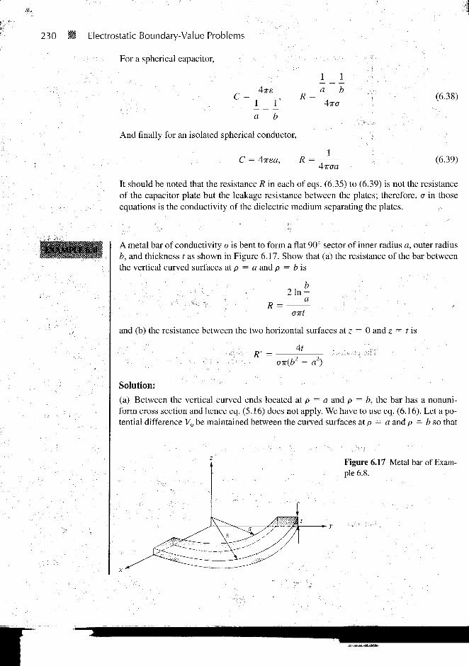
A metal bar of conductivity a is bent to form a flat 90° sector of inner radius a, outer radiusb, and thickness t as shown in Figure 6.17. Show that (a) the resistance of the bar betweenthe vertical curved surfaces at p = a and p = b is
R =oitt
and (b) the resistance between the two horizontal surfaces at z = 0 and z = t is
AtR' =
oir(b2 - a2)
Solution:(a) Between the vertical curved ends located at p = a and p = b, the bar has a nonuni-form cross section and hence eq. (5.16) does not apply. We have to use eq. (6.16). Let a po-tential difference Vo be maintained between the curved surfaces at p = a and p = b so that
Figure 6.17 Metal bar of Exam-ple 6.8.
r

6.5 RESISTANCE AND CAPACITANCE 231
V(p = a) = 0 and V(p = b) = Vo. We solve for V in Laplace's equation \2V = 0 in cylin-drical coordinates. Since V = V(p),
2 _\_d_( ^V'
P dp \ dp
As p = 0 is excluded, upon multiplying by p and integrating once, this becomes
o--A
or
dV _ A
; dp P ;
Integrating once again yields ?
V = Alnp + S
where A and 5 are constants of integration to be determined from the boundary conditions.
V(p = a) = 0 -> 0 = A In a + B or 5 = -A In a
V(p = b) = Vo -^ Vo = A In b + B = A In b - A In a = A In - or A = —a b
l n -
Hence ,
Thus
= A In p - A In a = A I n - = — l n -a b a• l n -
a
dp
J = aE, dS = -p
fTT/2
/ = J • dS =•*=° J -
p In —. a
dzpd(j> = - — -
In - In -a a
oirt
as required.

232 Electrostatic Boundary-Value Problems
(b) Let Vo be the potential difference between the two horizontal surfaces so thatV(z = 0) = 0 and V(z = i) = Vo. V = V(z), so Laplace's equation V2V = 0 becomes
dz2 = o
Integrating twice gives
: V = Az + B
We apply the boundary conditions to determine A and B:
V(z = 0) = 0 ^ 0 = 0 + 5 or B = 0
Hence,
V{z = t) = Vo->Vo=At or A =
V =
/ = J • dS =
Voa TT p
t ' 2 2
Thus
J = aE = az, dS = -p d<j> dp a.
p dcp dp
VOGIT (b2 - a2)
At
At
i
I o-K{b2 - a2)
Alternatively, for this case, the cross section of the bar is uniform between the hori-zontal surfaces at z.= 0 and z = t and eq. (5.16) holds. Hence,
a~(b- a1)
At
- a2)
as required.

6.5 RESISTANCE AND CAPACITANCE 233
n PRACTICE EXERCISE 6.8 »»SliIS§«8
A disc of thickness t has radius b and a central hole of radius a. Taking the conduc-;; tivity of the disc as a, find the resistance betweenis
I (a) The hole and the rim of the discft|V (b) The two flat sides of the disc
A coaxial cable contains an insulating material of conductivity a. If the radius of the centralwire is a and that of the sheath is b, show that the conductance of the cable per unit lengthis (see eq. (6.37))
- In b/a: Answer: (a) , (b)
2-Kta oir(b - a )
1= J • dS =
2*LoVo
In b/a
The resistance per unit length is
and the conductance per unit length is
Consider length L of the coaxial cable as shown in Figure 6.14. Let Vo be the potential dif-ference between the inner and outer conductors so that V(p = a) = 0 and V(p — b) = Vo
V and E can be found just as in part (a) of the last example. Hence:
-aVJ = aE = ° a p , dS = -pd<f> dz a p •
:: pmb/a ; • •
p dz. d(j>

234 U Electrostatic Boundary-Value Problems
PRACTICE EXERCISE 6.9
A coaxial cable contains an insulating material of conductivity ax in its upper halfand another material of conductivity a2 in its lower half (similar to the situation inFigure 6.19b). If the radius of the central wire is a and that of the sheath is b, showthat the leakage resistance of length £ of the cable is
Answer: Proof.
EXAMPLE 6.10Conducting spherical shells with radii a = 10 cm and b = 30 cm are maintained at a po-tential difference of 100 V such that V(r = b) = 0 and V(r = a) = 100 V. Determine Vand E in the region between the shells. If sr = 2.5 in the region, determine the total chargeinduced on the shells and the capacitance of the capacitor.
Solution: I
Consider the spherical shells shown in Figure 6.18. V depends only on r and henceLaplace's equation becomes
r2 dry dr
Since r =fc 0 in the region of interest, we multiply through by r2 to obtain
dr dr
Integrating once gives
dr
Figure 6.18 Potential V(r) due to conducting spherical shells.

6.5 RESISTANCE AND CAPACITANCE 235
or
Integrating again gives
dV _ Adr r2
V= + Br
As usual, constants A and B are determined from the boundarv conditions.
When r = b, V = 0 -^ 0 = + B or B = -b b
Hence
V = A1 1b ~ r
Also when r = a, V = Vo -> Vo = A1 1b ~ a
or
A =1 1b a
Thus
v=vnr ~ b
1 1a b
1 1r - |
ar
= eE • dS == 0 J0 =
47TEoS rVo
L-2-^r r2 sin 5 dd
a b
a b

236 B Electrostatic Boundary-Value Problems
The capacitance is easily determined as
Q =
Vo _ J _a b
which is the same as we obtained in eq. (6.32); there in Section 6.5, we assumed Q andfound the corresponding Vo, but here we assumed Vo and found the corresponding Q to de-termine C. Substituting a = 0.1 m, b = 0.3 m, Vo = 100 V yields
V = 10010 - 10/3 1 5 | r 3
Check: V2V = 0, V(r = 0.3 m) = 0, V(r = 0.1 m) = 100.
E =100
r2 [10 - 10/3]ar = —^ ar V/m
Q = ±4TT10"9 (2.5) • (100)
36?r 10 - 10/3 ' ' '•= ±4.167 nC
The positive charge is induced on the inner shell; the negative charge is induced on theouter shell. Also
C =\Q\ _ 4.167 X 10"
100= 41.67 pF
PRACTICE EXERCISE 6.10
If Figure 6.19 represents the cross sections of two spherical capacitors, determinetheir capacitances. Let a = 1 mm, b = 3 mm, c = 2 mm, srl = 2.5. and er2 = 3.5.
Answer: (a) 0.53 pF, (b) 0.5 pF
Figure 6.19 For Practice Exer-cises 6.9, 6.10, and 6.12.
(a) (b)
6.5 RESISTANCE AND CAPACITANCE 237
fcXA.V In Section 6.5, it was mentioned that the capacitance C = Q/V of a capacitor can be foundby either assuming Q and finding V or by assuming V and finding Q. The former approachwas used in Section 6.5 while we have used the latter method in the last example. Usingthe latter method, derive eq. (6.22).
Solution:
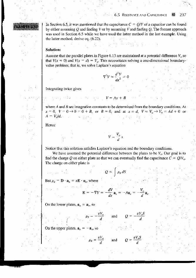
Assume that the parallel plates in Figure 6.13 are maintained at a potential difference Vo sothat V(x = 0) and V(x = d) = Vo. This necessitates solving a one-dimensional boundary-value problem; that is, we solve Laplace's equation
dx'
Integrating twice gives
where A and B are integration constants to be determined from the boundary conditions. Atx = 0, V = 0 -> 0 = 0 + B, or B = 0, and at x = d, V = Vo -> Vo = Ad + 0 or
Hence
Notice that this solution satisfies Laplace's equation and the boundary conditions.We have assumed the potential difference between the plates to be Vo. Our goal is to
find the charge Q on either plate so that we can eventually find the capacitance C = Q/Vo.The charge on either plate is
Q = As dS
But ps — D • an = eE • an, where
E = -VV= -~ax= -tdx
On the lower plates, an = ax, so
Ps =eVn
On the upper plates, an = -ax, so
d
and Q = —d
sVo sVoSPs = " V and Q = —T~

238 S Electrostatic Boundary-Value Problems
As expected, Q is equal but opposite on each plate. Thus
Vn d
which is in agreement with eq. (6.22).
N
5 PRACTICE EXERCISE 6.11H.
§/; Derive the formula for the capacitance C = Q/Vo of a cylindrical capacitor in eq.| (6.28) by assuming Vo and finding (?.
EXAMPLE <».12 Determine the capacitance of each of the capacitors in Figure 6.20. Take erl = 4, er2 = 6,d = 5 mm, 51 = 30 cm2.
Solution:
(a) Since D and E are normal to the dielectric interface, the capacitor in Figure 6.20(a) canbe treated as consisting of two capacitors Cx and C2 in series as in Figure 6.16(a).
P p V Op p V Op p C
*~ d/2 ~ d ' 2 ~ d
The total capacitor C is given by
C =CXC2 2EoS (erl£r2)
= 2
+ C2 d erl + er2
1 0 " 9 3 0 X 1 0 " 4 4 X 6
36TT 5 X 10"3
C = 25.46 pF10
w/2 w/2
(b)
Figure 6.20 For Example 6.12.
(6.12.1)

6.5 RESISTANCE AND CAPACITANCE 239
(b) In this case, D and E are parallel to the dielectric interface. We may treat the capacitoras consisting of two capacitors Cx and C2 in parallel (the same voltage across C\ and C2) asin Figure 6.16(b).
eos r l5/2 eoerlS _, sosr2S
Id ' Id
The total capacitance is
10"9 30 X 10"
~ 36TT 2 • (5 X 10~3)
C = 26.53 pF
er2)
10 (6.12.2)
Notice that when srl = er2 = er, eqs. (6.12.1) and (6.12.2) agree with eq. (6.22) as ex-pected.
PRACTICE EXERCISE 6.12
Determine the capacitance of 10 m length of the cylindrical capacitors shown inFigure 6.19. Take a = 1 mm, b = 3 mm, c = 2 mm, erl = 2.5, and er2 — 3.5.
Answer: (a) 1.41 nF, (b) 1.52 nF.
A cylindrical capacitor has radii a = 1 cm and b = 2.5 cm. If the space between the platesis filled with an inhomogeneous dielectric with sr = (10 + p)/p, where p is in centimeters,find the capacitance per meter of the capacitor.
Solution:
The procedure is the same as that taken in Section 6.5 except that eq. (6.27a) now becomes
V = -Q
2ireQsrpLdp= -
Q2iTBoL
dp
10 + p
-Q r dp = -Q2ire0L )b 10 + p 2irsoL
Q , 10 + b- m
In (10 + p)
2irsnL 10 +• a
240 Electrostatic Boundary-Value Problems
Thus the capacitance per meter is (L = 1 m)
„ Q10
C = 434.6 pF/m
= 2TT10- 9
36TT 12.5
A spherical capacitor with a = 1.5 cm, 6 = 4cm has an inhomogeneous dielectricjjj|ofe = lOSo/r. Calculate the capacitance of the capacitor.
K: Answer: 1.13 nF.
6.6 METHOD OF IMAGES
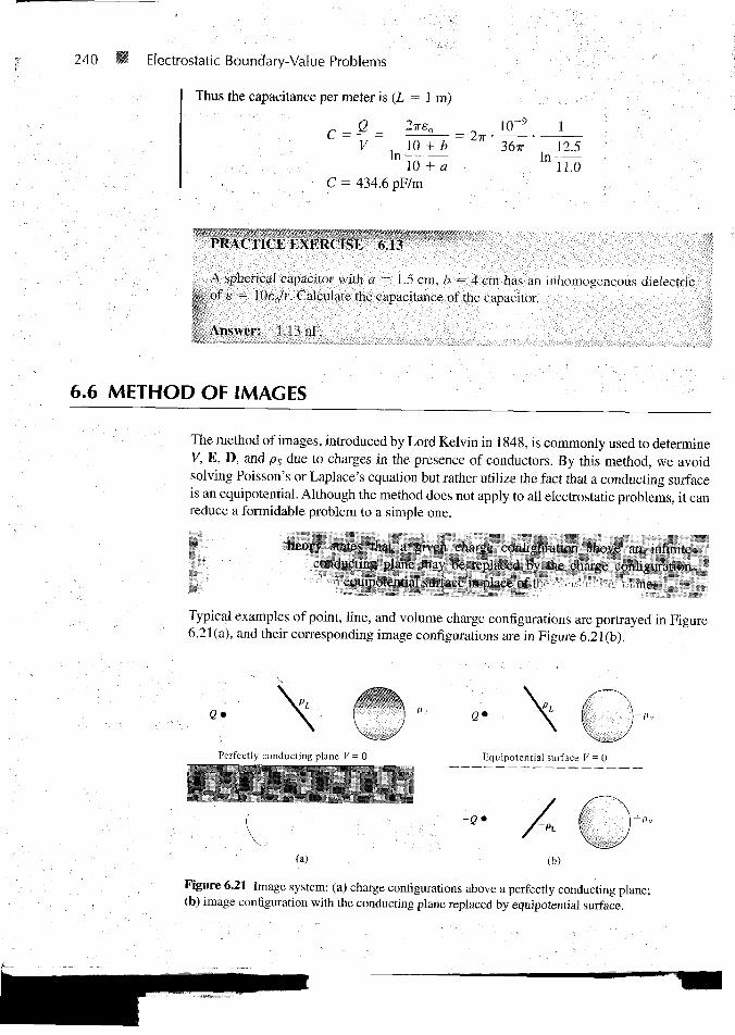
The method of images, introduced by Lord Kelvin in 1848, is commonly used to determineV, E, D, and ps due to charges in the presence of conductors. By this method, we avoidsolving Poisson's or Laplace's equation but rather utilize the fact that a conducting surfaceis an equipotential. Although the method does not apply to all electrostatic problems, it canreduce a formidable problem to a simple one.
lu-orx stales ilmi ti given charge ctinlijnirmion aho\e an inlinik'ciin-i plane max be replaced bx the charge conliguialioti
surface in place of 11 ' ' ' ,ie.
Typical examples of point, line, and volume charge configurations are portrayed in Figure6.21(a), and their corresponding image configurations are in Figure 6.21(b).
Equipotential surface V = 0
-Q*
(a)
Figure 6.21 Image system: (a) charge configurations above a perfectly conducting plane;(b) image configuration with the conducting plane replaced by equipotential surface.

6.6 METHOD OF IMAGES 241
In applying the image method, two conditions must always be satisfied:
1. The image charge(s) must be located in the conducting region.2. The image charge(s) must be located such that on the conducting surface(s) the po-
tential is zero or constant.
The first condition is necessary to satisfy Poisson's equation, and the second conditionensures that the boundary conditions are satisfied. Let us now apply the image theory totwo specific problems.
A. A Point Charge Above a Grounded Conducting PlaneConsider a point charge Q placed at a distance h from a perfect conducting plane of infiniteextent as in Figure 6.22(a). The image configuration is in Figure 6.22(b). The electric fieldat point P(x, y, z) is given by
E = E+ + E
The distance vectors r t and r2 are given by
r, = (x, y, z) - (0, 0, h) = (x, j , z - h)
. • ' . . r2 = (x, y> z) - (0, 0, -h) = (x, j , z + h)
so eq. (6.41) becomes
= J2_ f xax + yay + (z - fe)az _ xax + yay + (z + fe)a:2 + y2 + (z - h)2f2 [x2 + y2 + ( hff12
(6.40)
(6.41)
(6.42)
(6.43)
(6.44)
v= o/
P(x,y,z)
(a)
Figure 6.22 (a) Point charge and grounded conducting plane, (b) image configuration andfield lines.

Electrostatic Boundary-Value Problems
It should be noted that when z = 0, E has only the z-component, confirming that E isnormal to the conducting surface.
The potential at P is easily obtained from eq. (6.41) or (6.44) using V = -jE-dl.Thus
v=v+Q + ~Q
v =
4ireor1 4irsor2
Q
(6.45)
:o {[x2 + y2 + (z ~ hff2 [x2 + y2 + (z + h)2f
for z a 0 and V = 0 for z < 0 . Note that V(z = 0) = 0.The surface charge density of the induced charge can also be obtained from eq. (6.44) as
ps - Dn - eJLn
-Qh(6.46)
h2f2
The total induced charge on the conducting plane is
Qi= PsdS =-Qhdxdy
By changing variables, p2 = x2 + y2, dx dy = p dp d4>-
Qi = ~ n3/2
(6.47)
(6.48)
Integrating over <j> gives 2ir, and letting p dp = —d (p2), we obtain
,2,1/2(6.49)
= -Q
as expected, because all flux lines terminating on the conductor would have terminated onthe image charge if the conductor were absent.
B. A Line Charge above a Grounded Conducting Plane
Consider an infinite charge with density pL C/m located at a distance h from the groundedconducting plane z = 0. The same image system of Figure 6.22(b) applies to the linecharge except that Q is replaced by pL. The infinite line charge pL may be assumed to be at

6.6 METHOD OF IMAGES "t 243
x = 0, z = h and the image — pL at x = 0, z = ~A so that the two are parallel to the y-axis.The electric field at point P is given (from eq. 4.21) by .
(6.50)
(6.51)
(6.52)
(6.53)
(6.54)
The distance vectors p t and
E =
p2 are
E + +
PL
2irsop
given
E_
-PL
Z " 1 ' 27T£0p2
by
p2 = (x, y, z) - (0, y, -h) = (x, 0, z + h)
so eq. (6.51) becomes
E =pL \xax + (z - h)az xax
27T£O L X2 + (Z - X2 + (z +
Again, notice that when z = 0, E has only the z-component, confirming that E is normal tothe conducting surface.
The potential at P is obtained from eq. (6.51) or (6.54) using V = -jE-dl. Thus
V = V+ + V-
= PL 12iT£0
PL , Pi- In —
ft lnp2 (6.55)
. "• • . . ' . ' 2 T T E O P 2
Substituting px = \pi\ and p2 = \p2\ in eqs. (6.52) and (6.53) into eq. (6.55) gives
1/2
(6.56)
for z > 0 and V = 0 for z < 0 . Note that V(z = 0) = 0.The surface charge induced on the conducting plane is given by
Ps = Dn = soEz
The induced charge per length on the conducting plane is
pLh f°° dxPi= psdx = —
, x2 + h2
(6.57)
(6.58)
By letting x = h tan a, eq. (6.58) becomes
\Pi =
pLh r da(6.59)
as expected.

244 Electrostatic Boundary-Value Problems
EXAMPLE 6.14 A point charge Q is located at point (a, 0, b) between two semiinfinite conducting planesintersecting at right angles as in Figure 6.23. Determine the potential at point P(x, y, z) andthe force on Q.
Solution:
The image configuration is shown in Figure 6.24. Three image charges are necessary tosatisfy the conditions in Section 6.6. From Figure 6.24(a), the potential at point P(x, y, z) isthe superposition of the potentials at P due to the four point charges; that is,
V = Q rir2 >4
where
r4 = [{x-af
From Figure 6.24(b), the net force on Q
F = F, + F , + F3
n = [(x - a)2 +y2 + (z- b)2]1'2
r2 = [(x + a)2 + y 2 + (z- bf]yl
2 + (z + bf]m
2 + (z + bf]m
r3 = [(x + a)2
F2
Q2 Q2
4wso(2bf
Q2
47reo(2a)2 +
^3/2
Q2(2aax + 2baz)
4Treo[(2a)2 + {Ibfr2-, 3/2
{a2 + b2),2-v3/2 , 2 I az
The electric field due to this system can be determined similarly and the charge induced onthe planes can also be found.
Figure 6.23 Point charge between two semiinfiniteconducting planes.
o

6.6 METHOD OF IMAGES 245
" = o ,, »P(x,y,z)
(a) (b)
Figure 6.24 Determining (a) the potential at P, and (b) the force on charge Q.
In general, when the method of images is used for a system consisting of a pointcharge between two semiinfinite conducting planes inclined at an angle (/> (in degrees), thenumber of images is given by
because the charge and its images all lie on a circle. For example, when <j> = 180°, N = 1as in the case of Figure 6.22; for 0 = 90°, N = 3 as in the case of Figure 6.23; and for(j> = 60°, we expect AT = 5 as shown in Figure 6.25.
-Q Figure 6.25 Point charge between two semiinfiniteconducting walls inclined at <j> = 60° to each.
-Q -Q
+Q

246 Electrostatic Boundary-Value Problems
PRACTICE EXERCISE 6.14
If the point charge Q — 10 nC in Figure 6.25 is 10 cm away from point O and alongthe line bisecting <t> = 60°, find the magnitude of the force on Q due to the chargeinduced on the conducting walls.
A n s w e r : 6 0 . 5 3 / i N . . n ,; :;,.,... ---;•;::• :-iy:;:.-.;••->;;v,.ia:.s>:i,,SESs«i:
1. Boundary-value problems are those in which the potentials at the boundaries of a regionare specified and we are to determine the potential field within the region. They aresolved using Poisson's equation if pv =£ 0 or Laplace's equation if pv = 0.
2. In a nonhomogeneous region, Poisson's equation is
V • e VV = -pv
For a homogeneous region, e is independent of space variables. Poisson'becomes . ;
's equation
V2V = - ^
In a charge-free region (pv = 0), Poisson's equation becomes Laplace's equation;that is,
v2y = o
3. We solve the differential equation resulting from Poisson's or Laplace's equation by in-tegrating twice if V depends on one variable or by the method of separation of variablesif Vis a function of more than one variable. We then apply the prescribed boundary con-ditions to obtain a unique solution.
4. The uniqueness theorem states that if V satisfies Poisson's or Laplace's equation and theprescribed boundary condition, V is the only possible solution for that given problem.This enables us to find the solution to a given problem via any expedient means becausewe are assured of one, and only one, solution.
5. The problem of finding the resistance R of an object or the capacitance C of a capacitormay be treated as a boundary-value problem. To determine R, we assume a potentialdifference Vo between the ends of the object, solve Laplace's equation, find/ = / aE • dS, and obtain R = VJI. Similarly, to determine C, we assume a potentialdifference of Vo between the plates of the capacitor, solve Laplace's equation, findQ = / eE • dS, and obtain C = Q/Vo.
6. A boundary-value problem involving an infinite conducting plane or wedge may besolved using the method of images. This basically entails replacing the charge configu-ration by itself, its image, and an equipotential surface in place of the conducting plane.Thus the original problem is replaced by "an image problem," which is solved usingtechniques covered in Chapters 4 and 5. -, • •
REVIEW QUESTIONS 247
iREVIEW QUESTIONS
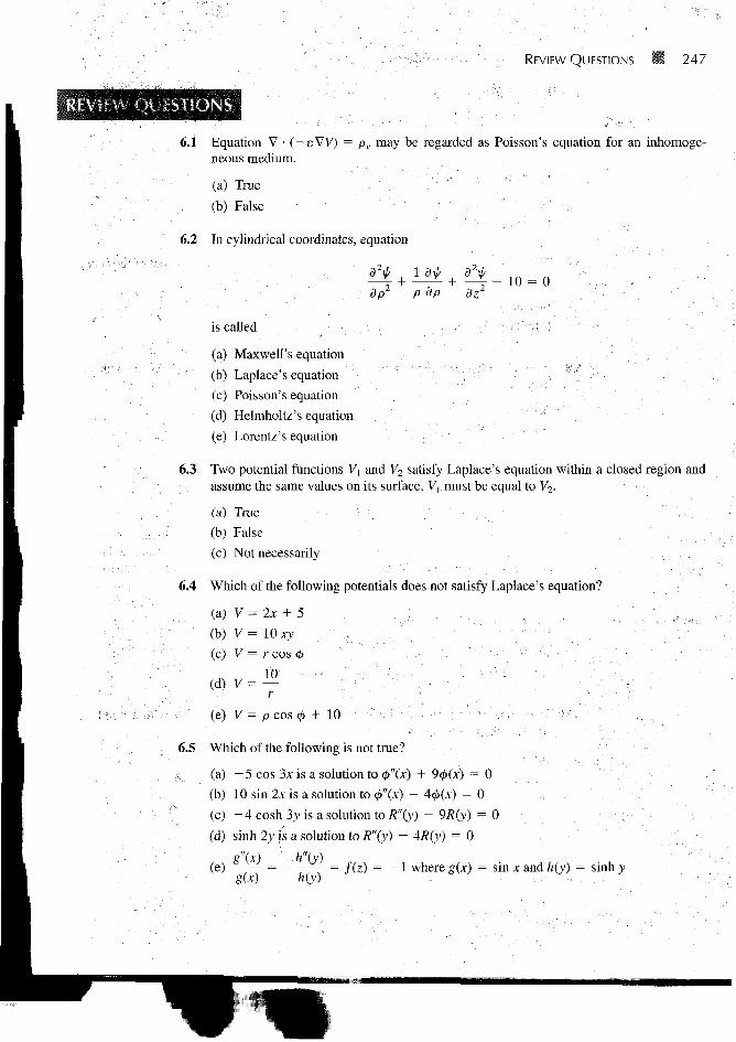
6.1 Equation V • ( —sVV) = pv may be regarded as Poisson's equation for an inhomoge-neous medium.
( a ) T r u e : • • • " ' " " " •
(b) False
6.2 In cylindrical coordinates, equation
+dp P dp + 10 = 0
is called . '•--'• ' l )
(a) Maxwell's equation
(b) Laplace's equation '""'•
(c) Poisson's equation
(d) Helmholtz's equation
(e) Lorentz's equation
6.3 Two potential functions Vi and V2 satisfy Laplace's equation within a closed region andassume the same values on its surface. Vx must be equal to V2.
(a) True . . ! '
(b) False
(c) Not necessarily
6.4 Which of the following potentials does not satisfy Laplace's equation?
( a ) V = 2x + 5 . . , • • , ; • ..,,.
(b) V= 10 xy ' , :
(c) V = r cos <j> " •
(e) V = p cos <$> + 10 ~ : ' - .-..- • :.' :
6.5 Which of the following is not true?
(a) - 5 cos 3x is a solution to 0"(x) + 90(x) = 0
(b) 10 sin 2x is a solution to <j)"(x) — 4cf>(x) = 0
(c) - 4 cosh 3y is a solution to ^"(y) - 9R(y) = 0
. (d) sinh 2y is a solution to R"(y) - 4R(y) = 0
(e) —-— = ——— = f(z) = - 1 where g(x) = sin x and h(y) = sinhyg(x) h(y)

248 H Electrostatic Boundary-Value Problems
6.6 If Vi = XlY1 is a product solution of Laplace's equation, which of these are not solutionsof Laplace's equation?
(a) -
(b) XyYy + 2xy
(c) X^ - x + y
(d)X1 + Y1
(e) (Xi - 2){YX + 3)
6.7 The capacitance of a capacitor filled by a linear dielectric is independent of the charge onthe plates and the potential difference between the plates.
(a) True
(b) False • . . - i : ; ,. ' -.
6.8 A parallel-plate capacitor connected to a battery stores twice as much charge with a givendielectric as it does with air as dielectric, the susceptibility of the dielectric is
(a) 0
(b) I •
(c) 2
(d) 3 v
(e) 4
6.9 A potential difference Vo is applied to a mercury column in a cylindrical container. Themercury is now poured into another cylindrical container of half the radius and the samepotential difference Vo applied across the ends. As a result of this change of space, the re-sistance will be increased . . .. •• . .
(a) 2 times
(b) 4 times
(c) 8 times , .
(d) 16 times
6.10 Two conducting plates are inclined at an angle 30° to each other with a point chargebetween them. The number of image charges is
(a) 12 / ' • " : : V " \
(b) 11
, ^ 6 - • ' " ' • • •
, (d) 5
(e) 3
Answers: 6.1a, 6.2c, 6.3a, 6.4c, 6.5b, 6.6d,e, 6.7a, 6.8b, 6.9d, 6.10b.

PROBLEMS
PROBLEMS6.1 In free space, V = 6xy2z + 8. At point P(\, 2, - 5 ) , find E and pv.
6.2 Two infinitely large conducting plates are located at x = 1 and x = 4. The space between
them is free space with charge distribution — nC/m3. Find Vatx = 2 if V(l) = —50V• I < O7T
and V(4) = 50 V. ,: - ; . -
6.3 The region between x = 0 and x = d is free space and has pv = po(x — d)ld. IfV(x = 0) = 0 and V(x = d) = Vo, find: (a) V and E, (b) the surface charge densities atx = 0 and x = d.
6.4 Show that the exact solution of the equation
• • / • • ' ' dx2 ~ m
0 <x < L
subject to
V(x = 0) = Vl V(x = L) = V2
/(/x) d\t, d\o Jo
(a) V, = x2 + y2 - 2z + 10
(c), V3 = pz sin <j> + p
6.7 Show that the following potentials satisfy Laplace's equation.
(a) V = e ""cos 13y sinh
249
6.5 A certain material occupies the space between two conducting slabs located at y =± 2 cm. When heated, the material emits electrons such that pv = 50(1 — y2) ^C/m3. Ifthe slabs are both held at 30 kV, find the potential distribution within the slabs. Takee = 3en. .
6.6 Determine which of the following potential field distributions satisfy Laplace's equation.

250 Electrostatic Boundary-Value Problems
d = 2 mm
'• = d) = Vn
V(z = 0) = 0
Figure 6.26 For Problem 6.11.
1
6.8 Show that E = (Ex, Ey, Ez) satisfies Laplace's equation.
6.9 Let V = (A cos nx + B sin nx)(Ceny + De~ny), where A, B, C, and £> are constants.Show that V satisfies Laplace's equation. . >
6.10 The potential field V = 2x2yz — y3z exists in a dielectric medium having e = 2eo.(a) Does V satisfy Laplace's equation? (b) Calculate the total charge within the unit cube0 < x,y,z < 1 m.
6.11 Consider the conducting plates shown in Figure 6.26. If V(z = 0) = 0 andV(z = 2 mm) = 50 V, determine V, E, and D in the dielectric region (er = 1.5) betweenthe plates and ps on the plates.
6.12 The cylindrical-capacitor whose cross section is in Figure 6.27 has inner and outer radii of5 mm and 15 mm, respectively. If V(p = 5 mm) = 100 V and V(p = 1 5 mm) = 0 V,calculate V, E, and D at p = 10 mm and ps on each plate. Take er = 2.0.
6.13 Concentric cylinders p = 2 cm and p = 6 cm are maintained at V = 60 V andV = - 2 0 V, respectively. Calculate V, E, and D at p = 4 cm.
6.14 The region between concentric spherical conducting shells r = 0.5 m and r = 1 m ischarge free. If V(r = 0.5) = - 5 0 V and V(r = 1) = 50 V, determine the potential dis-tribution and the electric field strength in the region between the shells.
6.15 Find V and E at (3, 0, 4) due to the two conducting cones of infinite extent shown inFigure 6.28.
Figure 6.27 Cylindrical capacitor of Problem 6.12.

PROBLEMS 251
V= 100 V
t
Figure 6.28 Conducting cones of Problem6.15.
*6.16 The inner and outer electrodes of a diode are coaxial cylinders of radii a = 0.6 m andb = 30 mm, respectively. The inner electrode is maintained at 70 V while the outer elec-trode is grounded, (a) Assuming that the length of the electrodes € ^> a, b and ignoringthe effects of space charge, calculate the potential at p = 15 mm. (b) If an electron is in-jected radially through a small hole in the inner electrode with velocity 107 m/s, find itsvelocity at p = 15mm.
6.17 Another method of finding the capacitance of a capacitor is using energy considerations,that is
C =2WE
vi
Using this approach, derive eqs. (6.22), (6.28), and (6.32).
6.18 An electrode with a hyperbolic shape (xy = 4) is placed above an earthed right-anglecorner as in Figure 6.29. Calculate V and E at point (1, 2, 0) when the electrode is con-nected to a 20-V source.
*6.19 Solve Laplace's equation for the two-dimensional electrostatic systems of Figure 6.30 andfind the potential V(x, y).
*6.20 Find the potential V(x, y) due to the two-dimensional systems of Figure 6.31.
6.21 By letting V(p, '#) = R(p)4>(4>) be the solution of Laplace's equation in a region wherep # 0, show that the separated differential equations for R and <P are

- xy = 4Figure 6.29 For Problem 6.18.
•v = o-
v=vo
(a)
Figure 6.30 For Problem 6.19.
(b) (c)
252
(0
Figure 6.31 For Problem 6.20.
• v = o
~v=o
(b)

PROBLEMS 253
and
where X is the separation constant.
4>" + X * = 0
6.22 A potential in spherical coordinates is a function of r and 8 but not <j>. Assuming thatV(r, 6) = R(r)F(6), obtain the separated differential equations for R and F in a region forwhich pv = 0.
6.23 Show that the resistance of the bar of Figure 6.17 between the vertical ends located at4> = 0 and <p = T /2 is
R =lot In bla
*6.24 Show that the resistance of the sector of a spherical shell of conductivity a, with crosssection shown in Figure 6.32 (where 0 < <$> < 2TT), between its base is
R =1 1 1
2-7TCT(1 — c o s ex.) i a b
*6.25 A hollow conducting hemisphere of radius a is buried with its flat face lying flush with theearth surface thereby serving as an earthing electrode. If the conductivity of earth is a,show that the leakage conductance between the electrode and earth is 2iraa.
6.26 The cross section of an electric fuse is shown in Figure 6.33. If the fuse is made of copperand of thickness 1.5 mm, calculate its resistance.
6.27 In an integrated circuit, a capacitor is formed by growing a silicon dioxide layer (s r = 4)of thickness 1 .m over the conducting silicon substrate and covering it with a metal elec-trode of area 5. Determine S if a capacitance of 2 nF is desired.
6.28 The parallel-plate capacitor of Figure 6.34 is quarter-filled with mica (e r = 6). Find thecapacitance of the capacitor.
Figure 6.32 For Problem 6.24.

254 11 Electrostatic Boundary-Value Problems
4 cm 4 cm
3 cm
M •
1 cmTf
<* •
4 cm
Figure 6.33 For Problem 6.26.
*6.29 An air-filled parallel plate capacitor of length L, width a, and plate separation d has its platesmaintained at constant potential difference Vo. If a dielectric slab of dielectric constant er isslid between the plates and is withdrawn until only a length x remains between the plates asin Figure 6.35, show that the force tending to restore the slab to its original position is
F =eo(er - 1) a Vj
Id
6.30 A parallel-plate capacitor has plate area 200 cm2 and plate separation 3 mm. The chargedensity is 1 /xC/m2 with air as dielectric. Find
(a) The capacitance of the capacitor
(b) The voltage between the plates
(c) The force with which the plates attract each other
6.31 Two conducting plates are placed at z = — 2 cm and z = 2 cm and are, respectively,maintained at potentials 0 and 200 V. Assuming that the plates are separated by apolypropylene (e = 2.25eo). Calculate: (a) the potential at the middle of the plates,(b) the surface charge densities at the plates.
6.32 Two conducting parallel plates are separated by a dielectric material with e = 5.6e0 andthickness 0.64 mm. Assume that each plate has an area of 80 cm2. If the potential field dis-tribution between the plates is V = 3x + Ay - \2z + 6 kV, determine: (a) the capaci-tance of the capacitor, (b) the potential difference between the plates.
Figure 6.34 For Problem 6.28.,10 cm2
2 mm

:. PROBLEMS • 255
Figure 6.35 For Problem 6.29.
6.33 The space between spherical conducting shells r = 5 cm and r = 10 cm is filled with adielectric material for which s = 2.25eo. The two shells are maintained at a potential dif-ference of 80 V. (a) Find the capacitance of the system, (b) Calculate the charge density onshell r = 5 cm.
6.34 Concentric shells r = 20 cm and r = 30 cm are held at V = 0 and V = 50, respectively.If the space between them is filled with dielectric material (e = 3.1e0, a = 10~12 S/m),find: (a) V, E, and D, (b) the charge densities on the shells, (c) the leakage resistance.
6.35 A spherical capacitor has inner radius a and outer radius d. Concentric with the sphericalconductors and lying between them is a spherical shell of outer radius c and inner radiusb. If the regions d < r < c,c < r < b, and b < r < a are filled with materials with per-mittivites eu e2, and e3, respectively, determine the capacitance of the system.
6.36 Determine the capacitance of a conducting sphere of radius 5 cm deeply immersed in seawater (er = 80).
6.37 A conducting sphere of radius 2 cm is surrounded by a concentric conducting sphere ofradius 5 cm. If the space between the spheres is filled with sodium chloride (er = 5.9),calculate the capacitance of the system.
*6.38 In an ink-jet printer the drops are charged by surrounding the jet of radius 20 fim with aconcentric cylinder of radius 600 /jm as in Figure 6.36. Calculate the minimum voltagerequired to generate a charge 50 fC on the drop if the length of the jet inside the cylinderis 100 /xm. Take e = eo.
6.39 A given length of a cable, the capacitance of which is 10 /xF/km with a resistance of insu-lation of 100 Mil/km, is charged to a voltage of 100 V. How long does it take the voltageto drop to 50 V?
Liquidreservior r-
A
\liquid jet
Figure 6.36 Simplified geometry of an ink-jetprinter; for Problem 6.38.
drop
J

256 Electrostatic Boundary-Value Problems
Figure 6.37 For Problem 6.40.
6.40 The capacitance per unit length of a two-wire transmission line shown in Figure 6.37 isgiven by
C =•we
cosh2a
Determine the conductance per unit length.
*6.41 A spherical capacitor has an inner conductor of radius a carrying charge Q and maintainedat zero potential. If the outer conductor contracts from a radius b to c under internalforces, prove that the work performed by the electric field as a result of the contraction is
W =Q\b - c)
8-irebc
*6.42 A parallel-plate capacitor has its plates at x = 0, d and the space between the plates is
filled with an inhomogeneous material with permittivity e = e0 1 H— I. If the plate atV dj
x = d is maintained at Vo while the plate at x = 0 is grounded, find:(a) VandE(b) P(c) pps at x = 0, d
6.43 A spherical capacitor has inner radius a and outer radius b and filled with an inhomoge-neous dielectric with e = eok/r2. Show that the capacitance of the capacitor is
C =b - a
6.44 A cylindrical capacitor with inner radius a and outer radius b is filled with an inhomoge-neous dielectric having e = eok/p, where A; is a constant. Calculate the capacitance perunit length of the capacitor.
6.45 If the earth is regarded a spherical capacitor, what is its capacitance? Assume the radius ofthe earth to be approximately 6370 km.

PROBLEMS 257
6.46 A point charge of 10 nC is located at point P(0, 0, 3) while the conducting plane z = 0 isgrounded. Calculate
(a) V and Eat R(6,3,5) '(b) The force on the charge due to induced charge on the plane.
6.47 Two point charges of 3 nC and - 4 nC are placed, respectively, at (0, 0, 1 m) and(0, 0, 2 m) while an infinite conducting plane is at z = 0. Determine
(a) The total charge induced on the plane(b) The magnitude of the force of attraction between the charges and the plane
6.48 Two point charges of 50 nC and - 2 0 nC are located at ( - 3 , 2, 4) and (1, 0, 5) above theconducting ground plane z = 2. Calculate (a) the surface charge density at (7, —2, 2),(b) D at (3, 4, 8), and (c) D at (1, 1, 1).
*6.49 A point charge of 10 jttC is located at (1, 1, 1), and the positive portions of the coordinateplanes are occupied by three mutually perpendicular plane conductors maintained at zeropotential. Find the force on the charge due to the conductors.
6.50 A point charge Q is placed between two earthed intersecting conducting planes that are in-clined at 45° to each other. Determine the number of image charges and their locations.
6.51 Infinite line x = 3, z = 4 carries 16 nC/m and is located in free space above the conduct-ing plane z = 0. (a) Find E at (2, — 2, 3). (b) Calculate the induced surface charge densityon the conducting plane at (5, — 6, 0).
6.52 In free space, infinite planes y = A and y = 8 carry charges 20 nC/m2 and 30 nC/m2, re-spectively. If plane y = 2 is grounded, calculate E at P(0, 0, 0) and Q(-4, 6, 2).

PART 3
MAGNETOSTATICS

Chapter 7
MAGNETOSTATIC FIELDS
No honest man can be all things to all people.
—ABRAHAM LINCOLN
7.1 INTRODUCTION
In Chapters 4 to 6, we limited our discussions to static electric fields characterized byE or D. We now focus our attention on static magnetic fields, which are characterizedby H or B. There are similarities and dissimilarities between electric and magnetic fields.As E and D are related according to D = eE for linear material space, H and B arerelated according to B = pR. Table 7.1 further shows the analogy between electric andmagnetic field quantities. Some of the magnetic field quantities will be introduced laterin this chapter, and others will be presented in the next. The analogy is presented hereto show that most of the equations we have derived for the electric fields may be readilyused to obtain corresponding equations for magnetic fields if the equivalent analo-gous quantities are substituted. This way it does not appear as if we are learning newconcepts.
A definite link between electric and magnetic fields was established by Oersted1 in1820. As we have noticed, an electrostatic field is produced by static or stationary charges.If the charges are moving with constant velocity, a static magnetic (or magnetostatic) fieldis produced. A magnetostatic field is produced by a constant current flow (or directcurrent). This current flow may be due to magnetization currents as in permanent magnets,electron-beam currents as in vacuum tubes, or conduction currents as in current-carryingwires. In this chapter, we consider magnetic fields in free space due to direct current. Mag-netostatic fields in material space are covered in Chapter 8.
Our study of magnetostatics is not a dispensable luxury but an indispensable necessity.r The development of the motors, transformers, microphones, compasses, telephone bell
ringers, television focusing controls, advertising displays, magnetically levitated high-speed vehicles, memory stores, magnetic separators, and so on, involve magnetic phenom-ena and play an important role in our everyday life.2
Hans Christian Oersted (1777-1851), a Danish professor of physics, after 13 years of frustratingefforts discovered that electricity could produce magnetism.2Various applications of magnetism can be found in J. K. Watson, Applications of Magnetism. NewYork: John Wiley & Sons, 1980.
^ : , '.-."•• 2 6 1

262 Magnetostatic Fields
TABLE 7.1 Analogy between Electric and Magnetic Fields*
Term
Basic laws
Force law
Source element
Field intensity
Flux density
Relationship between fields
Potentials
\ • - • , , * • •
Flux
Energy density
Poisson's equation
F
fF
dQ
E
D
D
E
v ••
yy
/ =
wE
V2
Electric
2,224ire2 '
D • dS = g e n c
= gEi
= | ( V / m )
y= - (C/m 2 )
= sE
= - Wf Pidl
J Airsr
= / D • dS
= Q = CV
- I . . .
E
<P H
F =gu =
H =
B =
H =
A -
y =
v =
Wm =
V2A
Magnetic
4,r«2
• d\ = / e n c
gu X B
\ (A/m)
y— (Wb/m2)
- vym (j = o)
f nidij 47ri?
J B - d S
L/L f
i
"A similar analogy can be found in R. S. Elliot, "Electromagnetic theory: asimplified representation," IEEE Trans. Educ, vol. E-24, no. 4, Nov. 1981,pp. 294-296.
There are two major laws governing magnetostatic fields: (1) Biot-Savart's law,3 and(2) Ampere's circuit law.4 Like Coulomb's law, Biot-Savart's law is the general law ofmagnetostatics. Just as Gauss's law is a special case of Coulomb's law, Ampere's law is aspecial case of Biot-Savart's law and is easily applied in problems involving symmetricalcurrent distribution. The two laws of magnetostatics are stated and applied first; theirderivation is provided later in the chapter.
3The experiments and analyses of the effect of a current element were carried out by Ampere and byJean-Baptiste and Felix Savart, around 1820.4Andre Marie Ampere (1775-1836), a French physicist, developed Oersted's discovery and intro-duced the concept of current element and the force between current elements.

7.2 BIOT-SAVART'S LAW 263
7.2 BIOT-SAVART'S LAW
Biot-Savart's law states that the magnetic field intensity dll produced at a point P,as shown in Figure 7.1, by the differential current clement / ill is proportional to theproduct / dl and the sine of the angle a between the clement and the line joining P tothe element and is inversely proportional to the square of the distance K between Pand the element.
That is,
or
dH =
/ dl sin a~ R2
kl dl sin a
R~2
(7.1)
(7.2)
where k is the constant of proportionality. In SI units, k = l/4ir, so eq. (7.2) becomes
/ dl sin adH =
4TTRZ(7.3)
From the definition of cross product in eq. (1.21), it is easy to notice that eq. (7.3) isbetter put in vector form as
dH =Idl X a« Idl XR
(7.4)
where R = |R| and aR = R/R. Thus the direction of d¥L can be determined by the right-hand rule with the right-hand thumb pointing in the direction of the current, the right-handfingers encircling the wire in the direction of dH as shown in Figure 7.2(a). Alternatively,we can use the right-handed screw rule to determine the direction of dH: with the screwplaced along the wire and pointed in the direction of current flow, the direction of advanceof the screw is the direction of dH as in Figure 7.2(b).
Figure 7.1 magnetic field dH at P due to currentelement I dl.
dH (inward)

264
(a)
Figure 7.2 Determining the direction of dH using(a) the right-hand rule, or (b) the right-handed screwrule.
It is customary to represent the direction of the magnetic field intensity H (or current/) by a small circle with a dot or cross sign depending on whether H (or I) is out of, or into,the page as illustrated in Figure 7.3.
Just as we can have different charge configurations (see Figure 4.5), we can have dif-ferent current distributions: line current, surface current, and volume current as shown inFigure 7.4. If we define K as the surface current density (in amperes/meter) and J as thevolume current density (in amperes/meter square), the source elements are related as
(7.5)
Thus in terms of the distributed current sources, the Biot-Savart law as in eq. (7.4)becomes
H
H =
H
Id\ X aR (line current)
KdSXaR
;— (surface current)4TTR2
J dv X aR
z— (volume current)4wR2
(7.6)
(7.7)
(7.8)
As an example, let us apply eq. (7.6) to determine the field due to a straight currentcarrying filamentary conductor of finite length AB as in Figure 7.5. We assume that theconductor is along the z-axis with its upper and lower ends respectively subtending angles
H (or /) is out H (or /) is in Figure 7.3 Conventional representation of H (or I) (a) out of^ the page and (b) into the page.
(a) (b)

7.2 BIOT-SAVART'S LAW 265
(a) (b) (c)
Figure 7.4 Current distributions: (a) line current, (b) surfacecurrent, (c) volume current.
a2 and a} at P, the point at which H is to be determined. Particular note should be taken ofthis assumption as the formula to be derived will have to be applied accordingly. If we con-sider the contribution dH at P due to an element dl at (0, 0, z),
d¥l =Idl X R
4TTR3
But dl = dz az and R = pap - zaz, so
dl X R = P dz i
Hence,
IpdzH
(7.9)
(7.10)
(7.11)
Figure 7.5 Field at point P due to a straight filamen-tary conductor.
H (into the page)

266 w Magnetostatic Fields
Letting z = p cot a, dz — -p cosec2 a da, and eq. (7.11) becomes
H1 f"2 p2 cosec2 a da
p3 cosec3 a
sin a da
4ir
I
4irp
or
I H = - — (cos a2 - cos4irp
(7.12)
This expression is generally applicable for any straight filamentary conductor of finitelength. Notice from eq. (7.12) that H is always along the unit vector a^ (i.e., along concen-tric circular paths) irrespective of the length of the wire or the point of interest P. As aspecial case, when the conductor is semiinfinite (with respect to P) so that point A is now at(9(0, 0, 0) while B is at (0, 0, °°); a, = 90°, a2 = 0°, and eq. (7.12) becomes
H =4?rp
(7.13)
Another special case is when the conductor is infinite in length. For this case, point A is at(0, 0, -oo) while B is at (0, 0, °°); a, = 180°, a2 = 0°, so eq. (7.12) reduces to
H =2xp
(7.14)
To find unit vector a0 in eqs. (7.12) to (7.14) is not always easy. A simple approach is to de-termine SJ, from
= &e X a (7.15)
where af is a unit vector along the line current and ap is a unit vector along the perpendic-ular line from the line current to the field point.
EXAMPLE 7.1 The conducting triangular loop in Figure 7.6(a) carries a current of 10 A. Find H at (0, 0, 5)due to side i of the loop.
Solution:
This example illustrates how eq. (7.12) is applied to any straight, thin, current-carryingconductor. The key point to keep in mind in applying eq. (7.12) is figuring out a b a2, p,and a^. To find H at (0, 0, 5) due to side 1 of the loop in Figure 7.6(a), consider Figure

7.2 BIOT-SAVART'S LAW 267
.©
(a)
Figure 7.6 For Example 7.1: (a) conducting triangularloop, (b) side 1 of the loop.
7.6(b), where side 1 is treated as a straight conductor. Notice that we join the point of in-terest (0, 0, 5) to the beginning and end of the line current. Observe that au a2, and p areassigned in the same manner as in Figure 7.5 on which eq. (7.12) is based.
cos a, = cos 90° = 0, cos a2 =V29'
To determine a0 is often the hardest part of applying eq. (7.12). According to eq. (7.15),a{ = BX and ap = az, so
= ar az = - a v
Hence,
Hi = irP (cos *2 -cos
= — 59.1av mA/m

268 Magnetostatic Fields
PRACTICE EXERCISE 7.1
Find H at (0. 0, 5) due to side 3 of the triangular loop in Figure 7.6(a).
Answer: -30.63a, + 3().63av mA/m.
EXAMPLE 7.2Find H at ( - 3 , 4, 0) due to the current filament shown in Figure 7.7(a).
Solution:Let H = Hx + Hz, where Hx and H;, are the contributions to the magnetic field intensity atP( — 3, 4, 0) due to the portions of the filament along x and z, respectively.
H7 =4TTP
(cos a2 - cos
At P ( - 3 , 4, 0), p = (9 + 16)1/2 = 5, «! = 90°, a2 = 0°, and a , is obtained as a unitvector along the circular path through P on plane z = 0 as in Figure 7.7(b). The directionof a^ is determined using the right-handed screw rule or the right-hand rule. From thegeometry in Figure 7.7(b),
4 3a0 = sin 6 ax + cos 6 ay = — ax + — ay
Alternatively, we can determine a^ from eq. (7.15). At point P, a.? and ap are as illustratedin Figure 7.7(a) for Hz. Hence,
3= - a z X ( -- ax + - ayJ = - ax + - ay
4
5
(a) (b)
Figure 7.7 For Example 7.2: (a) current filament along semiinfinite x- andz-axes; a and ap for Hz only; (b) determining ap for Hz.

7.2 BIOT-SAVART'S LAW 269
as obtained before. Thus
4TT(5)
28.65ay mA/m
It should be noted that in this case a0 happens to be the negative of the regular a^ of cylin-drical coordinates. Hz could have also been obtained in cylindrical coordinates as
z 4TT(5)V " »'
= -47.75a,£ mA/m
Similarly, for Hx at P, p = 4, a2 = 0°, cos a, = 3/5, and a^ = az or a^ = ae X
ap = ax X ay = az. Hence,
Thus
or
= 23.88 a, mA/m
H = Hx + Uz = 38.2ax + 28.65ay + 23.88a, mA/m
H = -47.75a0 + 23.88a, mA/m
Notice that although the current filaments appear semiinfinite (they occupy the posi-tive z- and x-axes), it is only the filament along the £-axis that is semiinfinite with respectto point P. Thus Hz could have been found by using eq. (7.13), but the equation could nothave been used to find Hx because the filament along the x-axis is not semiinfinite withrespect to P.
PRACTICE EXERCISE 7.2
The positive v-axis (semiinfinite line with respect to the origin) carries a filamentarycurrent of 2 A in the —ay direction. Assume it is part of a large circuit. Find H at
(a) A(2, 3, 0)
(b) fl(3, 12, -4 )
Answer: (a) 145.8az mA/m, (b) 48.97a,. + 36.73a; mA/m.

270 H Magnetostatic Fields
EXAMPLE 7.3 A circular loop located on x2 + y2 = 9, z = 0 carries a direct current of 10 A along a$. De-termine H at (0, 0, 4) and (0, 0, -4 ) .
Solution:
Consider the circular loop shown in Figure 7.8(a). The magnetic field intensity dH at pointP(0, 0, h) contributed by current element / d\ is given by Biot-Savart's law:
A-KR3
where d\ = p d<j) a0, R = (0, 0, h) - (x, y, 0) = -pap + haz, and
d\ X R = 0 pd4> 0- p 0 h
= p/i az
Hence,
- = — — - (ph d<$> ap + p2 d<\> az) = dHp i4x[p + h ]
dHzaz
By symmetry, the contributions along ap add up to zero because the radial componentsproduced by pairs of current element 180° apart cancel. This may also be shown mathe-matically by writing ap in rectangular coordinate systems (i.e., ap = cos <f> ax + sin <j> ay).
P(0, 0, h)
Figure 7.8 For Example 7.3: (a) circular current loop, (b) flux lines dueto the current loop.

7.2 BIOT-SAVART'S LAW 271
Integrating cos <j> or sin $ over 0 < <j> < 2TT gives zero, thereby showing that Hp = 0.Thus
HIp
l0 4TT[P2 47T[p2 + h2f2
or
H2[p2 + h2f2
(a) Substituting/ = \0A,p = 3,h = 4 gives
H(0, 0, 4) = 1 0 ( 3 ) **„ = 0.36a7 A/m2[9 + 16]3/2
(b) Notice from rflXR above that if h is replaced by - h, the z-component of dH remainsthe same while the p-component still adds up to zero due to the axial symmetry of the loop.Hence
H(0, 0, -4 ) = H(0, 0,4) = 0.36az A/m
The flux lines due to the circular current loop are sketched in Figure 7.8(b).
PRACTICE EXERCISE 7.3
A thin ring of radius 5 cm is placed on plane z = 1 cm so that its center is at(0,0,1 cm). If the ring carries 50 mA along a^, find H at
(a) ( 0 , 0 , - l c m )
(b) (0,0, 10 cm)
Answer: (a) 400az mA/m, (b) 57.3az mA/m.
EXAMPLE 7.4A solenoid of length € and radius a consists of N turns of wire carrying current /. Show thatat point P along its axis,
H = — (cos 62 - cos 0,)az
where n = N/€, dl and d2 are the angles subtended at P by the end turns as illustrated inFigure 7.9. Also show that if £ ^> a, at the center of the solenoid,
H = nl&,

272 • Magnetostatic Fields
Figure 7.9 For Example 7.4; cross sectionof a solenoid.
Solution:
Consider the cross section of the solenoid as shown in Figure 7.9. Since the solenoid con-sists of circular loops, we apply the result of Example 7.3. The contribution to the magneticfield H at P by an element of the solenoid of length dz is
la n dzdH7 =
Idle?
2[a2 + z2]m ~ 2[a2 + z2f2
where dl = ndz = (Nit) dz. From Figure 7.9, tan 0 = alz\ that is,
dz = -a cosec2 0 dd = -[l + " ] sin 6 dd
Hence,
or
Thus
dHz = - — sin 0 dd
Hz = - — | sin 0 dO
H = — (cos 62 - cos di) az
as required. Substituting n = Nit, gives
NIH = — (cos 02 ~ c o s
At the center of the solenoid,
cos V7 =1/2
[a2 + (2/4]1 = -cos

7.3 AMPERE'S CIRCUIT LAW—MAXWELL'S EQUATION • 273
and
„ _2 + €2/4]1/2 z2[a2 + €2/4]
If € » aor02 = O°, 0, = 180°,
H
PRACTICE EXERCISE 7.4
If the solenoid of Figure 7.9 has 2,000 turns, a length of 75 cm, a radius of 5 cm, andcarries a current of 50 mA along a^, find H at
(a) (0,0, 0)
(b) (0, 0, 75 cm)
(c) (0,0,50 cm)
Answer: (a) 66.52az him, (b) 66.52a2 him, (c) 131.7az him.
.3 AMPERE'S CIRCUIT LAW—MAXWELL'S EQUATION
Ampere's circuit law states that the line integral of the tangential component of Haround a dosed path is the same as the net current /,.IK. enclosed by the path.
In other words, the circulation of H equals /enc; that is,
(7.16)
Ampere's law is similar to Gauss's law and it is easily applied to determine H when thecurrent distribution is symmetrical. It should be noted that eq. (7.16) always holds whetherthe current distribution is symmetrical or not but we can only use the equation to determineH when symmetrical current distribution exists. Ampere's law is a special case ofBiot-Savart's law; the former may be derived from the latter.
By applying Stoke's theorem to the left-hand side of eq. (7.16), we obtain
/ e n c = = ( V X H W S (7.17)

274 Magnetostatic Fields
But
4nc = J (7.18)
Comparing the surface integrals in eqs. (7.17) and (7.18) clearly reveals that
V X H = J (7.19)
This is the third Maxwell's equation to be derived; it is essentially Ampere's law in differ-ential (or point) form whereas eq. (7.16) is the integral form. From eq. (7.19), we shouldobserve that V X H = J + 0; that is, magnetostatic field is not conservative.
7.4 APPLICATIONS OF AMPERE'S LAW
We now apply Ampere's circuit law to determine H for some symmetrical current distri-butions as we did for Gauss's law. We will consider an infinite line current, an infinitecurrent sheet, and an infinitely long coaxial transmission line.
A. Infinite Line Current
Consider an infinitely long filamentary current / along the z-axis as in Figure 7.10. To de-termine H at an observation point P, we allow a closed path pass through P. This path, onwhich Ampere's law is to be applied, is known as an Amperian path (analogous to the termGaussian surface). We choose a concentric circle as the Amperian path in view ofeq. (7.14), which shows that H is constant provided p is constant. Since this path enclosesthe whole current /, according to Ampere's law
j pd<f> = 2irp
Amperian path
Figure 7.10 Ampere's law applied to an infinite filamentaryline current.

or
7.4 APPLICATIONS OF AMPERE'S LAW M 275
(7.20)
as expected from eq. (7.14).
B. Infinite Sheet of Current
Consider an infinite current sheet in the z = 0 plane. If the sheet has a uniform currentdensity K = Kyay A/m as shown in Figure 7.11, applying Ampere's law to the rectangularclosed path (Amperian path) gives
H • d\ = /enc = Kyb (7.21a)
To evaluate the integral, we first need to have an idea of what H is like. To achieve this, weregard the infinite sheet as comprising of filaments; dH above or below the sheet due to apair of filamentary currents can be found using eqs. (7.14) and (7.15). As evident in Figure7.11(b), the resultant dH has only an x-component. Also, H on one side of the sheet is thenegative of that on the other side. Due to the infinite extent of the sheet, the sheet can be re-garded as consisting of such filamentary pairs so that the characteristics of H for a pair arethe same for the infinite current sheets, that is,
JHoaxI ~Hoax
z > 0z < 0
(7.21b)
(a)
Figure 7.11 Application of Ampere's law to an infinite sheet: (a) closed path 1-2-3-4-1, (b) sym-metrical pair of current filaments with current along ay.
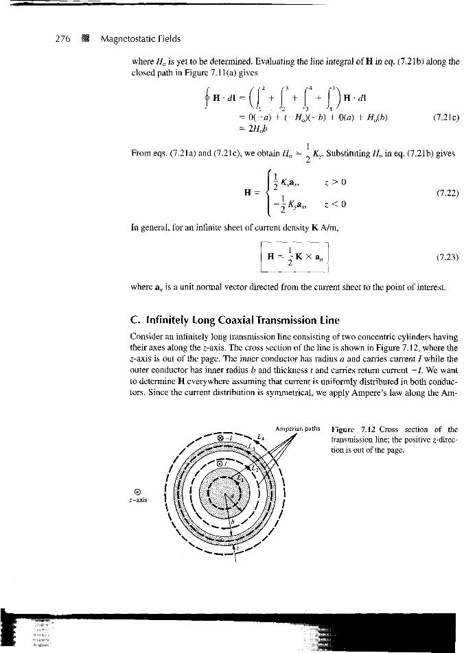
276 Magnetostatic Fields
where Ho is yet to be determined. Evaluating the line integral of H in eq. (7.21b) along theclosed path in Figure 7.11 (a) gives
U-dl = [ \ + + + j H • rflI h h M '
= 0 ( -a ) + (-Ho)(-b) + 0(fl) + Ho(b)= 2Hob
1
(7.21c)
From eqs. (7.21a) and (7.21c), we obtain Ho = — Ky. Substituting Ho in eq. (7.21b) gives
H = <z>0
(7.22)-~Kyax, z<0
In general, for an infinite sheet of current density K A/m,
(7.23)
where an is a unit normal vector directed from the current sheet to the point of interest.
C. Infinitely Long Coaxial Transmission Line
Consider an infinitely long transmission line consisting of two concentric cylinders havingtheir axes along the z-axis. The cross section of the line is shown in Figure 7.12, where thez-axis is out of the page. The inner conductor has radius a and carries current / while theouter conductor has inner radius b and thickness t and carries return current - / . We wantto determine H everywhere assuming that current is uniformly distributed in both conduc-tors. Since the current distribution is symmetrical, we apply Ampere's law along the Am-
©
Amperian paths Figure 7.12 Cross section of the4 yf transmission line; the positive ?-direc-
tion is out of the page.

jath,
:q. (7.26) ise use path L

278 Magnetostatic Fields
and J in this case is the current density (current per unit area) of the outer conductor and isalong -av that is,
J = -
Thus
ir[(b + if - b2] z
2TT rp
= / 1p2-b2
t2 + 2bt.
p dp d<f>
Substituting this in eq. (7.27a), we have
H -
For region p > 6 + t, we use path L4, getting
L4
or
Putting eqs. (7.25) to (7.28) together gives
(7.27b)
(7.28)
H = <
aw,,
2?rp
0,2bt
0 < p < a
a < p < Z?
b < p<b + t
p > b + t
(7.29)
The magnitude of H is sketched in Figure 7.13.Notice from these examples that the ability to take H from under the integral sign is
the key to using Ampere's law to determine H. In other words, Ampere's law can only beused to find H due to symmetric current distributions for which it is possible to find aclosed path over which H is constant in magnitude.

7.4 APPLICATIONS OF AMPERE'S LAW 279
Figure 7.13 Plot of H^ against p.
•U-
b b+t
EXAMPLE 7.5Planes 2 = 0 and z = 4 carry current K = -lOa* A/m and K = lOa* A/m, respectively.Determine H at
(a) (1,1,1)(b) (0, - 3 , 10)
Solution:
Let the parallel current sheets be as in Figure 7.14. Also let
H = Ho + H4
where Ho and H4 are the contributions due to the current sheets z = 0 and z = 4, respec-tively. We make use of eq. (7.23).
(a) At (1, 1, 1), which is between the plates (0 < z = 1 < 4),
Ho = 1/2 K X an = 1/2 (-10ax) X a, = 5av A/m
H4 = l / 2 K X a , = 1/2 (10ax) X (-a,) = 5ay A/m
Hence,
H = 10ay A/m
: = 4 Figure 7.14 For Example 7.5; parallel
» » « « M » B = t infinite current sheets.
y \® 8 8 8 8z = 0
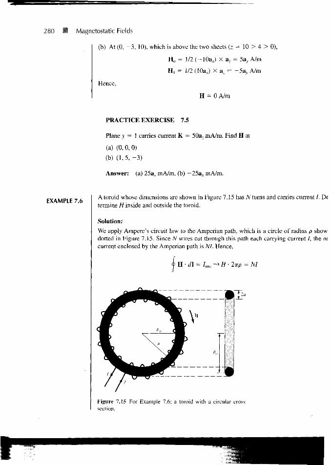
280 • Magnetostatic Fields
(b) At (0, - 3 , 10), which is above the two sheets (z = 10 > 4 > 0),
Ho = 1/2 ( - 10a*) X az = 5a, A/m
H4 = 1/2 (lOaJ X az = -5a y A/m
Hence,
H = 0 A/m
PRACTICE EXERCISE 7.5
Plane y = 1 carries current K = 50az mA/m. Find H at
(a) (0,0,0)
(b) (1 ,5 , -3 )
Answer: (a) 25ax mA/m, (b) — 25a* mA/m.
EXAMPLE 7.6A toroid whose dimensions are shown in Figure 7.15 has N turns and carries current /. Determine H inside and outside the toroid.
Solution:
We apply Ampere's circuit law to the Amperian path, which is a circle of radius p showdotted in Figure 7.15. Since N wires cut through this path each carrying current /, the n<current enclosed by the Amperian path is NI. Hence,
H • d\ = 7enc -> H • 2irp = M
Figure 7.15 For Example 7.6; a toroid with a circular crosssection.
7.5 MAGNETIC FLUX DENSITY—MAXWELL'S EQUATION • 281
or
H =NI
2irp'for po - a < p < po + a
where po is the mean radius of the toroid as shown in Figure 7.15. An approximate value ofHis
H,NI NI
approx 2irpo
Notice that this is the same as the formula obtained for H for points well inside a very longsolenoid (€ 5s> a). Thus a straight solenoid may be regarded as a special toroidal coil forwhich po —»co. Outside the toroid, the current enclosed by an Amperian path isNI - NI = 0 and hence H = 0.
PRACTICE EXERCISE 7.6
A toroid of circular cross section whose center is at the origin and axis the same asthe z-axis has 1000 turns with po - 10 cm, a = 1 cm. If the toroid carries a 100-mAcurrent, find \H\ at / \...,. / '
\ - * • • ' •
(a) (3 c m , - 4 cm, 0) • !>~ ' .
(b) (6 cm, 9 cm, 0)
Answer: (a) 0, (b) 147.1 A/m.
-.5 MAGNETIC FLUX DENSITY—MAXWELL'SEQUATION
The magnetic flux density B is similar to the electric flux density D. As D = soE in freespace, the magnetic flux density B is related to the magnetic field intensity H according to
(7.30)
where ^o is a constant known as the permeability of free space. The constant is inhenrys/meter (H/m) and has the value of
= 4TT X 10~7 H/m (7.31)
The precise definition of the magnetic field B, in terms of the magnetic force, will be givenin the next chapter.

282 Magnetostatic Fields
Figure 7.16 Magnetic flux lines due to a straightMagnetic flux lines wire with current coming out of the page.
The magnetic flux through a surface S is given by
(7.32)
where the magnetic flux f is in webers (Wb) and the magnetic flux density is inwebers/square meter (Wb/m2) or teslas.
The magnetic flux line is the path to which B is tangential at every point in a magneticfield. It is the line along which the needle of a magnetic compass will orient itself if placedin the magnetic field. For example, the magnetic flux lines due to a straight long wire areshown in Figure 7.16. The flux lines are determined using the same principle followed inSection 4.10 for the electric flux lines. The direction of B is taken as that indicated as"north" by the needle of the magnetic compass. Notice that each flux line is closed and hasno beginning or end. Though Figure 7.16 is for a straight, current-carrying conductor, it isgenerally true that magnetic flux lines are closed and do not cross each other regardless ofthe current distribution.
In an electrostatic field, the flux passing through a closed surface is the same as thecharge enclosed; that is, *P = §D • dS = Q. Thus it is possible to have an isolated electriccharge as shown in Figure 7.17(a), which also reveals that electric flux lines are not neces-sarily closed. Unlike electric flux lines, magnetic flux lines always close upon themselvesas in Figure 7.17(b). This is due to the fact that it is not possible to have isolated magnetic
closed surface, *• = Q
closed surface, f = 0
(a) (b)
Figure 7.17 Flux leaving a closed surface due to: (a) isolated electriccharge V = §s D • dS = Q, (b) magnetic charge, Y = §s B • dS = 0.
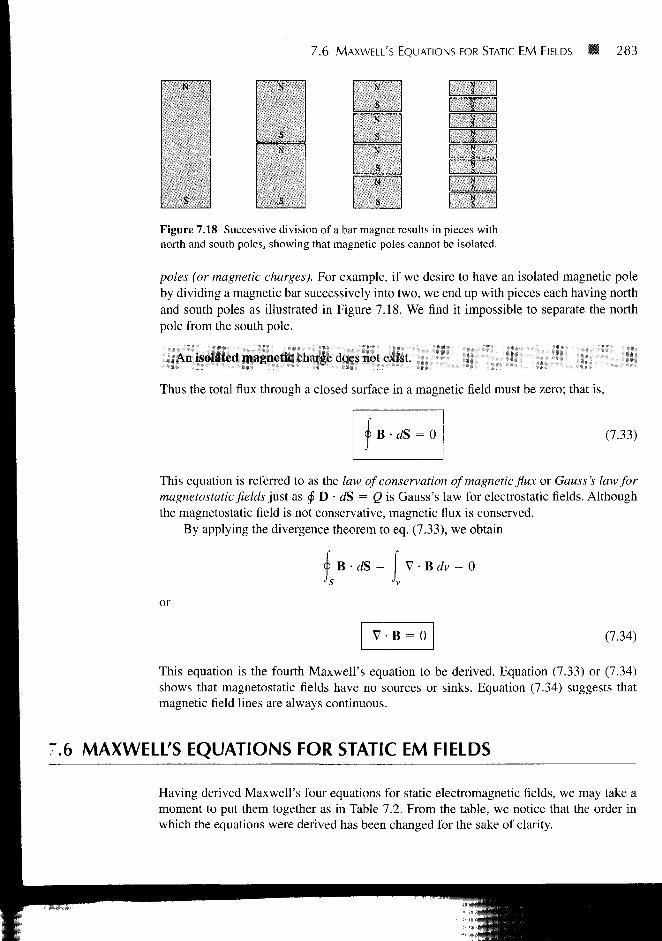
7.6 MAXWELL'S EQUATIONS FOR STATIC EM FIELDS 283
N
S
N
S
N
S
N
S
N
S
N
SN
S
s
BN
N'
N
N
Figure 7.18 Successive division of a bar magnet results in pieces withnorth and south poles, showing that magnetic poles cannot be isolated.
poles (or magnetic charges). For example, if we desire to have an isolated magnetic poleby dividing a magnetic bar successively into two, we end up with pieces each having northand south poles as illustrated in Figure 7.18. We find it impossible to separate the northpole from the south pole.
An isolated magnetic charge does not exist.
Thus the total flux through a closed surface in a magnetic field must be zero; that is,
(7.33)
This equation is referred to as the law of conservation of magnetic flux or Gauss's law formagnetostatic fields just as § D • dS = Q is Gauss's law for electrostatic fields. Althoughthe magnetostatic field is not conservative, magnetic flux is conserved.
By applying the divergence theorem to eq. (7.33), we obtain
B • dS = V • B dv = 0
or
V B = 0 (7.34)
This equation is the fourth Maxwell's equation to be derived. Equation (7.33) or (7.34)shows that magnetostatic fields have no sources or sinks. Equation (7.34) suggests thatmagnetic field lines are always continuous.
.6 MAXWELL'S EQUATIONS FOR STATIC EM FIELDS
Having derived Maxwell's four equations for static electromagnetic fields, we may take amoment to put them together as in Table 7.2. From the table, we notice that the order inwhich the equations were derived has been changed for the sake of clarity.

284 Magnetostatic Fields
TABLE 7.2 Maxwell's Equations for Static EM Fields
Differential (or Point) Form Integral Form Remarks
V • D = pv
V - B = 0
V X E = 0
V x H = J
D • dS = pv dv Gauss's law
B • dS =
E • d\ = '
Nonexistence of magneticmonopole
Conservativeness ofelectrostatic field
H • d\ = J • dS Ampere's law
The choice between differential and integral forms of the equations depends on agiven problem. It is evident from Table 7.2 that a vector field is defined completely byspecifying its curl and divergence. A field can only be electric or magnetic if it satisfies thecorresponding Maxwell's equations (see Problems 7.26 and 7.27). It should be noted thatMaxwell's equations as in Table 7.2 are only for static EM fields. As will be discussed inChapter 9, the divergence equations will remain the same for time-varying EM fields butthe curl equations will have to be modified.
7.7 MAGNETIC SCALAR AND VECTOR POTENTIALS
We recall that some electrostatic field problems were simplified by relating the electric po-tential V to the electric field intensity E (E = — VV). Similarly, we can define a potentialassociated with magnetostatic field B. In fact, the magnetic potential could be scalar Vm orvector A. To define Vm and A involves recalling two important identities (see Example 3.9and Practice Exercise 3.9):
V X (VV) = 0
V • (V X A) = 0
(7.35a)
(7.35b)
which must always hold for any scalar field V and vector field A.Just as E = - VV, we define the magnetic scalar potential Vm (in amperes) as related
to H according to
H = -VVm if J = 0 (7.36)
The condition attached to this equation is important and will be explained. Combining eq.(7.36) and eq. (7.19) gives
J = V X H = V X ( - VVm) = 0 (7.37)

7.7 MAGNETIC SCALAR AND VECTOR POTENTIALS 285
since Vm must satisfy the condition in eq. (7.35a). Thus the magnetic scalar potential Vm isonly defined in a region where J = 0 as in eq. (7.36). We should also note that Vm satisfiesLaplace's equation just as V does for electrostatic fields; hence,
V2Vm = 0, (J = 0) (7.38)
We know that for a magnetostatic field, V • B = 0 as stated in eq. (7.34). In order tosatisfy eqs. (7.34) and (7.35b) simultaneously, we can define the vector magnetic potentialA (in Wb/m) such that
B = V X A
Just as we defined
we can define
V =dQ
4ireor
(7.39)
(7.40)
for line current
for surface current
for volume current
(7.41)
(7.42)
(7.43)
Rather than obtaining eqs. (7.41) to (7.43) from eq. (7.40), an alternative approachwould be to obtain eqs. (7.41) to (7.43) from eqs. (7.6) to (7.8). For example, we can deriveeq. (7.41) from eq. (7.6) in conjunction with eq. (7.39). To do this, we write eq. (7.6) as
IdV X R
R3(7.44)
where R is the distance vector from the line element dV at the source point (x1, y', z') to thefield point (x, y, z) as shown in Figure 7.19 and R = |R|, that is,
R = |r - r'| = [(x - x'f + (y - y'f + (z - z'f]1 (7.45)
Hence,
v| 1\ =Rj
(x - x')ax + (y - / )a y R
[(x - x'f - y'f + (z - z')T2

286 • Magnetostatic Fields
R = r r'
Figure 7.19 Illustration of the source point(*', y', z') and the field point (x, y, z).
(x, y, z)
or
R R(7.46)
where the differentiation is with respect to x, y, and z. Substituting this into eq. (7.44), weobtain
B= - - M IdV X v ( -4TT R
(7.47)
We apply the vector identity
V X ( / F ) = / V X F + ( V / ) X F (7.48)
where/is a scalar field and F is a vector field. Taking / = \IR and F = dV, we have
Since V operates with respect to (x, y, z) while dV is a function of (x\ y', z'), V X dV = 0.Hence,
(7.49)
(7.50)
With this equation, eq. (7.47) reduces to
B = V x4irR
Comparing eq. (7.50) with eq. (7.39) shows that
verifying eq. (7.41).

7.7 MAGNETIC SCALAR AND VECTOR POTENTIALS • 287
By substituting eq. (7.39) into eq. (7.32) and applying Stokes's theorem, we obtain
= B • dS = (V X A) • dS = <P A • d\
4or
(7.51)
Thus the magnetic flux through a given area can be found using either eq. (7.32) or (7.51).Also, the magnetic field can be determined using either Vm or A; the choice is dictated bythe nature of the given problem except that Vm can only be used in a source-free region.The use of the magnetic vector potential provides a powerful, elegant approach to solvingEM problems, particularly those relating to antennas. As we shall notice in Chapter 13, itis more convenient to find B by first finding A in antenna problems.
EXAMPLE 7.7 Given the magnetic vector potential A = —p2/4 az Wb/m, calculate the total magnetic fluxcrossing the surface <f> = -ir/2, 1 < p < 2 m , 0 < z < 5 m .
Solution:
We can solve this problem in two different ways: using eq. (7.32) or eq. (7.51).
Method 1:
B = V x A = —-* a0 = J a0,op 2dS = dp dz a0
Hence,
TP = j B • dS = -
¥ = 3.75 Wb
1p dp dz = — p
z=0 •>=
(5) =15
Method 2:We use
<p = I A • d\ = f i + v2 + r3 + v4'L
where L is the path bounding surface S; V 1( f 2, ¥3, and V4 are, respectively, the evalua-tions of /A • d\ along the segments of L labeled 1 to 4 in Figure 7.20. Since A has only a2-component,
¥>, = 0 = y 3

288 I I Magnetostatic Fields
5 -
4 -
3 -
2 -
1 -
©'
©
©L
1 *
That is,
i rr\ 2
Figure 7.20 For Example 7.7.
= 3.75 Wb
as obtained previously. Note that the direction of the path L must agree with that of dS.
PRACTICE EXERCISE 7.7
A current distribution gives rise to the vector magnetic potential A = xzy&x +
y2xay — 4xyzaz Wb/m. Calculate
(a) B a t ( - 1 , 2 , 5)
(b) The flux through the surface defined b y z = 1 , 0 ^ x ^ 1 , - 1 < y < 4
Answer: (a) 20ax + 40ay + 3az Wb/m2, (b) 20 Wb.
EXAMPLE 7.8If plane z = 0 carries uniform current K = Kyay,
H1/2 Kyax,-l/2Kvax,
>0<0
This was obtained in Section 7.4 using Ampere's law. Obtain this by using the concept ofvector magnetic potential.

7.7 MAGNETIC SCALAR AND VECTOR POTENTIALS • 289
Solution:
Consider the current sheet as in Figure 7.21. From eq. (7.42),
lxoKdSdA =
A-KR
In this problem, K = Kyay, dS = dx' dy', and for z > 0,
R = |R| = |(0, 0, z) - (x',y',0)\= \ix'f + (y'f + z2]112 (7.8.1)
where the primed coordinates are for the source point while the unprimed coordinates arefor the field point. It is necessary (and customary) to distinguish between the two points toavoid confusion (see Figure 7.19). Hence
dA =dx' dy' ay
4TT[(X')2 + (y'f + z2]'f + z2]1'2
dB = V X dA = —— d Ay ax
dzjxoKyz dx' dy' ax
B
4ir[(x')2 + (y'f + z2]3'2
H0Kzax r f °° dx' dy'2n3/2 (7.8.2)
In the integrand, we may change coordinates from Cartesian to cylindrical for convenienceso that
Hence
B =4ir
fioKyz
4ir
jxoKyzax
P' d4>' dp'
y=o v=o;2TT I [(p')
- 1
too2 + z2y p'=0
/ o 2f or z > 0
By simply replacing z by ~z in eq. (7.8.2) and following the same procedure, we obtain
is
H = — l ax, for z < 0

290 • Magnetostatic Fields
Figure 7.21 For Example 7.8; infinitecurrent sheet.
*• y
PRACTICE EXERCISE 7.8
Repeat Example 7.8 by using Biot-Savart's law to determine H at points (0,0, h)and (0,0, -h).
7.8 DERIVATION OF BIOT-SAVART'S LAWAND AMPERE'S LAW
Both Biot-Savart's law and Ampere's law may be derived using the concept of magneticvector potential. The derivation will involve the use of the vector identities in eq. (7.48)and
V X V X A = V(V • A) - V2A (7.52)
Since Biot-Savart's law as given in eq. (7.4) is basically on line current, we begin ourderivation with eqs. (7.39) and (7.41); that is,
4TTR 4TT R(7.53)
where R is as denned in eq. (7.45). If the vector identity in eq. (7.48) is applied by lettingF = dl and / = \IR, eq. (7.53) becomes
(7.54)
Since V operates with respect to (x, y, z) and dl' is a function of (xr, y', z'), V X dl' = 0.Also
- = [(x - x'f + (y- y'f + (z - z')2]R
-1/2 (7.55)

7.8 DERIVATION OF BIOT-SAVART'S LAW AND AMPERE'S LAW 291
j_l = (x - x')ax + (y- y')ay + (z - z')az = _a«
R [(x - x'f + (y~ y'Y-, 3/2 (7.56)
where a^ is a unit vector from the source point to the field point. Thus eq. (7.54) (upondropping the prime in d\') becomes
4TT ) L R2
which is Biot-Savart's law.Using the identity in eq. (7.52) with eq. (7.39), we obtain
V X B = V(V • A) - V2A
It can be shown that for a static magnetic field
V-A = 0
so that upon replacing B with /xoH and using eq. (7.19), eq. (7.58) becomes
V2A = -AIOV X H
or
V2A = -i
(7.57)
(7.58)
(7.59)
(7.60)
which is called the vector Poisson's equation. It is similar to Poisson's equation(V2V = ~pvle) in electrostatics. In Cartesian coordinates, eq. (7.60) may be decomposedinto three scalar equations:
V2AX = ~
V2Ay = - (7.61)
which may be regarded as the scalar Poisson's equations.It can also be shown that Ampere's circuit law is consistent with our definition of the
magnetic vector potential. From Stokes's theorem and eq. (7.39),
H d\ = V X H • dS
V X (V X A)-dS
From eqs. (7.52), (7.59), and (7.60),
VxVxA=-V2A =
(7.62)

•2 I '."agnetostatic Fields
Substituting this into eq. (7.62) yields
H d\ = J • dS = I
which is Ampere's circuit law.
SUMMARY 1. The basic laws (Biot-Savart's and Ampere's) that govern magnetostatic fields are dis-cussed. Biot-Savart's law, which is similar to Coulomb's law, states that the magneticfield intensity dH at r due to current element / d\ at r' is
dRId\ X R
(in A/m)
where R = r — r' and R = |R|. For surface or volume current distribution, we replace/ d\ with K dS or J dv respectively; that is,
Id\ = = Jdv
2. Ampere's circuit law, which is similar to Gauss's law, states that the circulation of Haround a closed path is equal to the current enclosed by the path; that is,
or
V X H = J
= IeiK = \ J - d S
(third Maxwell's equation to be derived).
When current distribution is symmetric so that an Amperian path (on which His constant) can be found, Ampere's law is useful in determining H; that is,
= Im or H^ =*enc
3. The magnetic flux through a surface S is given by
f = \B-dS (inWb)
where B is the magnetic flux density in Wb/m2. In free space,
where fio = 4ir X 10 7 H/m = permeability of free space.4. Since an isolated or free magnetic monopole does not exist, the net magnetic flux
through a closed surface is zero;
f = <t B • dS = 0

REVIEW QUESTIONS '•- 293
or
V • B = 0 (fourth Maxwell's equation to be derived).
5. At this point, all four Maxwell's equations for static EM fields have been derived,namely:
V • D = Pv
V-B = 0
V X E = 0
V X H = J
6. The magnetic scalar potential Vm is defined as
H = - W m if J = 0
and the magnetic vector potential A as
B = V X A
where V • A = 0. With the definition of A, the magnetic flux through a surface S can befound from
V = | A • d\'L
where L is the closed path defining surface S (see Figure 3.20). Rather than usingBiot-Savart's law, the magnetic field due to a current distribution may be found usingA, a powerful approach that is particularly useful in antenna theory. For a currentelement / d\ at r', the magnetic vector potential at r is
A =A-KR '
R= r - r ' l
7. Elements of similarity between electric and magnetic fields exist. Some of these arelisted in Table 7.1. Corresponding to Poisson's equation V2V = —pvle, for example, is
V2A = -nJ
7.1 One of the following is not a source of magnetostatic fields:
(a) A dc current in a wire
(b) A permanent magnet
(c) An accelerated charge
(d) An electric field linearly changing with time
(e) A charged disk rotating at uniform speed

294 Magnetostatic Fields
7.2 Identify the configuration in Figure 7.22 that is not a correct representation of /and H.
7.3 Consider points A, B, C, D, and £ on a circle of radius 2 as shown in Figure 7.23. Theitems in the right list are the values of a^ at different points on the circle. Match theseitems with the points in the list on the left.
(a)
(b)
(c)
(d)
(e)
A
B
C
D
77h
(1)
(ii)(iii)
(iv)
(v)
(vi)
(vii)
(viii)
ax
- a *a>- a v
a, + ay
V2- a x - a.
- a x + ay
ax - ay
7.4 The z-axis carries filamentary current of IOTT A along az. Which of these is incorrect?
(a) H = - a , A / m at (0 ,5 ,0)
(b) H = a^ A/m at (5, TT/4, 0)
(c) H = -0.8ax - 0 .6a } , a t ( -3 ,4 , 0)
(d) H = - a 0 a t ( 5 , 3ir/2, 0)
7.5 Plane y = 0 carries a uniform current of 30az niA/m. At (1, 10, —2), the magnetic fieldintensity is
(a) —\5&xm£Jm
(b) 15
(a)
(d)
(b) (c)
H© ©
'O ©© ©
(e)
Figure 7.22 For Review Question 7.2.

IREVIEW QUESTIONS ~Ji 295
Figure 7.23 For Review Question 7.3.
(c) 477.5a,,/xA/m
(d) 18.85avnA/m
(e) None of the above
7.6 For the currents and closed paths of Figure 7.24, calculate the value of j>L H • d\.
7.7 Which of these statements is not characteristic of a static magnetic field?
(a) It is solenoidal.
(b) It is conservative.
(c) It has no sinks or sources.
(d) Magnetic flux lines are always closed.
(e) The total number of flux lines entering a given region is equal to the total number offlux lines leaving the region.
Si 30 A
Figure 7.24 For Review Question 7.6.
30 A
(c) (d)

296 Magnetostatic Fields
Figure 7.25 For Review Question 7.10.
Volume
7.8 Two identical coaxial circular coils carry the same current / but in opposite direc-tions. The magnitude of the magnetic field B at a point on the axis midway between thecoils is
(a) Zero
(b) The same as that produced by one coil
(c) Twice that produced by one coil
(d) Half that produced by one coil.
7.9 One of these equations is not Maxwell's equation for a static electromagnetic field in alinear homogeneous medium.
(a) V • B = 0
(b) V X D = 0(c) 0 B • d\ = nJ(d) § D • dS = Q
(e) V2A = nJ
7.10 Two bar magnets with their north poles have strength Qml = 20 A • m andQm2 = 10 A • m (magnetic charges) are placed inside a volume as shown in Figure 7.25.The magnetic flux leaving the volume is
(a) 200 Wb
(b) 30 Wb
(c) 10 Wb
(d) OWb
(e) - lOWb
Answers: 7.1c, 7.2c, 7.3 (a)-(ii), (b)-(vi), (c)-(i), (d)-(v), (e)-(iii), 7.4d, 7.5a, 7.6 (a) 10 A,(b) - 2 0 A, (c) 0, (d) - 1 0 A, 7.7b, 7.8a, 7.9e, 7.10d.
PROBLEMS7.1 (a) State Biot-Savart's law
(b) The y- and z-axes, respectively, carry filamentary currents 10 A along ay and 20 Aalong -az. Find H at ( - 3 , 4, 5).
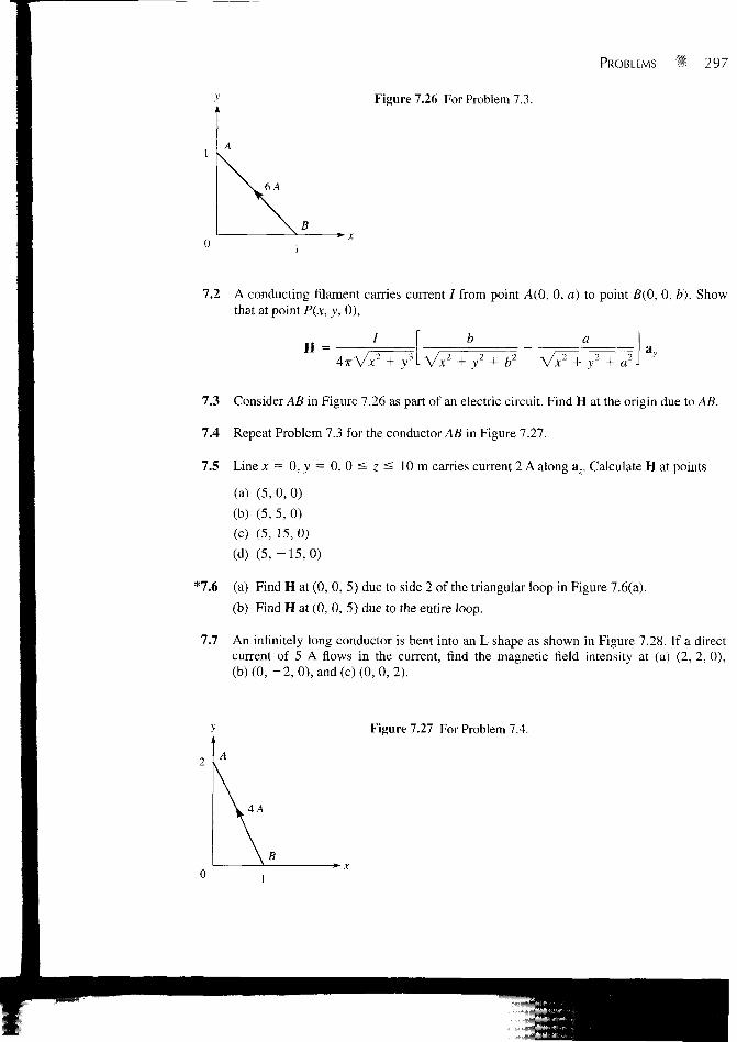
PROBLEMS « 297
Figure 7.26 For Problem 7.3.
7.2 A conducting filament carries current / from point A(0, 0, a) to point 5(0, 0, b). Showthat at point P(x, y, 0),
H =Vx^
7.3 Consider AB in Figure 7.26 as part of an electric circuit. Find H at the origin due to AB.
7.4 Repeat Problem 7.3 for the conductor AB in Figure 7.27.
7.5 Line x = 0, y = 0, 0 < z £ 10m carries current 2 A along az. Calculate H at points
(a) (5, 0, 0)
(b) (5, 5, 0)
(c) (5, 15, 0)
(d) ( 5 , - 1 5 , 0 )
*7.6 (a) Find H at (0, 0, 5) due to side 2 of the triangular loop in Figure 7.6(a).
(b) Find H at (0, 0, 5) due to the entire loop.
7.7 An infinitely long conductor is bent into an L shape as shown in Figure 7.28. If a directcurrent of 5 A flows in the current, find the magnetic field intensity at (a) (2, 2, 0),(b)(0, - 2 , 0), and (c) (0,0, 2).
Figure 7.27 For Problem 7.4.
4A

298 Magnetostatic Fields
Figure 7.28 Current filament for Problem 7.7.
5 A
5A
7.8 Find H at the center C of an equilateral triangular loop of side 4 m carrying 5 A of currentas in Figure 7.29.
7.9 A rectangular loop carrying 10 A of current is placed on z = 0 plane as shown in Figure7.30. Evaluate H at
(a) (2, 2, 0)
(b) (4, 2, 0)
(c) (4, 8, 0)
(d) (0, 0, 2)
7.10 A square conducting loop of side 2a lies in the z = 0 plane and carries a current / in thecounterclockwise direction. Show that at the center of the loop
H•wa
*7.11 (a) A filamentary loop carrying current / is bent to assume the shape of a regular polygonof n sides. Show that at the center of the polygon
nl . irH = sin —
2irr n
where r is the radius of the circle circumscribed by the polygon.
(b) Apply this to cases when n = 3 and n = 4 and see if your results agree with those forthe triangular loop of Problem 7.8 and the square loop of Problem 7.10, respectively.
Figure 7.29 Equilateral triangular loop forProblem 7.8.

PROBLEMS • 299
Figure 7.30 Rectangular loop of Problem 7.9.
(c) As n becomes large, show that the result of part (a) becomes that of the circular loopof Example 7.3.
7.12 For the filamentary loop shown in Figure 7.31, find the magnetic field strength at O.
7.13 Two identical current loops have their centers at (0, 0, 0) and (0, 0, 4) and their axes thesame as the z-axis (so that the "Helmholtz coil" is formed). If each loop has radius 2 mand carries current 5 A in a , calculate H at
(a) (0,0,0)(b) (0,0,2)
7.14 A 3-cm-long solenoid carries a current of 400 mA. If the solenoid is to produce a mag-netic flux density of 5 mWb/m , how many turns of wire are needed?
7.15 A solenoid of radius 4 mm and length 2 cm has 150 turns/m and carries current 500 mA.Find: (a) [H at the center, (b) |H | at the ends of the solenoid.
7.16 Plane x = 10 carries current 100 mA/m along az while line x = 1, y = —2 carries fila-mentary current 20TT mA along a r Determine H at (4, 3, 2).
7.17 (a) State Ampere's circuit law.
(b) A hollow conducting cylinder has inner radius a and outer radius b and carries current/ along the positive z-direction. Find H everywhere.
10 A
100 cm
10 A
Figure 7.31 Filamentary loop of Problem 7.12; not drawn to scale.

300 Magnetostatic Fields
7.18 (a) An infinitely long solid conductor of radius a is placed along the z-axis. If the con-ductor carries current / i n the + z direction, show that
H = 2a<t>2ira
within the conductor. Find the corresponding current density,
(b) If / = 3 A and a = 2 cm in part (a), find H at (0, 1 cm, 0) and (0, 4 cm, 0).
(7.19 If H = yax - xay A/m on plane z = 0, (a) determine the current density and (b) verify" Ampere's law by taking the circulation of H around the edge of the rectangle
Z = 0, 0 < x < 3, - 1 < y < 4.
7.20 In a certain conducting region, - . • - , • •
H = yz(x2 + y2)ax - y2xzay + 4x2y2az A/m .
(a) Determine J at (5, 2 , - 3 )
(b) Find the current passing through x = —1,0 < y,z < 2
(c) Show that V • B = 0
7.21 An infinitely long filamentary wire carries a current of 2 A in the +z-direction.Calculate
(a) B a t ( - 3 , 4 , 7 ) " - . . • • • • ..;•••.•
(b) The flux through the square loop described by 2 < p < 6, 0 < z ^ 4, <£ = 90°
7.22 The electric motor shown in Figure 7.32 has field
106
H = s in 2<j> a A/m
Calculate the flux per pole passing through the air gap if the axial length of the pole is20 cm.
7.23 Consider the two-wire transmission line whose cross section is illustrated in Figure 7.33.Each wire is of radius 2 cm and the wires are separated 10 cm. The wire centered at (0, 0)
Figure 7.32 Electric motor pole of Problem 7.22.
armature

PROBLEMS 301
4 c m±KJ-10 cm-
Figure 7.33 Two-wire line of Problem7.23.
carries current 5 A while the other centered at (10 cm, 0) carries the return current. FindHat
(a) (5 cm, 0)
(b) (10 cm, 5 cm)
7.24 Determine the magnetic flux through a rectangular loop (a X b) due to an infinitely longconductor carrying current / as shown in Figure 7.34. The loop and the straight conductorsare separated by distance d.
*7.25 A brass ring with triangular cross section encircles a very long straight wire concentricallyas in Figure 7.35. If the wire carries a current /, show that the total number of magneticflux lines in the ring is
r = b — a Ina + b
2-wb L b
Calculate V if a = 30 cm, b = 10 cm, h = 5 cm, and / = 10 A.
7.26 Consider the following arbitrary fields. Find out which of them can possibly representelectrostatic or magnetostatic field in free space.
(a) A = y cos axax + (y + e~x)az
(b) B = — ap
(c) C = r2 sin 6 a0
Figure 7.34 For Problem 7.24
I ,<

302 • Magnetostatic Fields
hv.
- Brass ring
Figure 7.35 Cross section of a brass ring enclosing a longstraight wire; for Problem 7.25.
7.27 Reconsider the previous problem for the following fields.
(a) D = y2zax + 2{x + \)yzay - (JC + l)z2az
,, , _ (z + 1) , , s i n 0(b) E = cos 4> aD H
P P
(c) F = — (2 cos 6 ar + sin d ae)
7.28 For a current distribution in free space,
A = {2x2y + yz)ax + {xy2 - xz3)ay - (6xyz ~ 2jc2.y2 )az Wb/m
(a) Calculate B.
(b) Find the magnetic flux through a loop described by x = 1, 0 < y, z < 2.
(c) Show that V • A = 0 and V • B = 0.
7.29 The magnetic vector potential of a current distribution in free space is given by
A = 15<?~p sin <j> az Wb/m
Find H at (3, ir/4, - 10). Calculate the flux through p = 5, 0 £ 0 < w/2, 0 < z < 10.
7.30 A conductor of radius a carries a uniform current with J = Joaz. Show that the magneticvector potential for p > a is
A = --)iaJop2az
7.31 An infinitely long conductor of radius a is placed such that its axis is along the z-axis. Thevector magnetic potential, due to a direct current Io flowing along a, in the conductor, isgiven by
A = ~ fxo(x2 + y2) az Wb/m
Find the corresponding H. Confirm your result using Ampere's law.

PROBLEMS • 303
7.32 The magnetic vector potential of two parallel infinite straight current filaments in freespace carrying equal current / in opposite direction is
JX.1 d - pA = — In a,
2TT p
where d is the separation distance between the filaments (with one filament placed alongthe z-axis). Find the corresponding magnetic flux density B.
7.33 Find the current density J to
in free space.
A = — az Wb/mP
7.34 Prove that the magnetic scalar potential at (0, 0, z) due to a circular loop of radius ashown in Figure 7.8(a) is
V m = - | 1 -
*7.35 A coaxial transmission line is constructed such that the radius of the inner conductor is aand the outer conductor has radii 3a and 4a. Find the vector magnetic potential within theouter conductor. Assume Az = 0 for p = 3a.
7.36 The z-axis carries a filamentary current 12 A along az. Calculate Vm at (4, 30°, - 2 ) ifVm = Oat(10, 60°, 7).
7.37 Plane z = — 2 carries a current of 50ay A/m. If Vm = 0 at the origin, find Vm at
(a) ( - 2 , 0 , 5 )
(b) (10, 3, 1)
7.38 Prove in cylindrical coordinates that
(a) V X (VV) = 0
(b) V • (V X A) = 0
7.39 IfR = r - r' and/? = |R|, show that
R R fl3
where V and V are del operators with respect to (x, y, z) and (x', y', z), respectively.

Chapter 8
MAGNETIC FORCES, MATERIALS,AND DEVICES
Do all the good you can,By all the means you can,In all the ways you can,In all the places you can,At all the times you can,To all the people you can,As long as ever you can.
—JOHN WESLEY
8.1 INTRODUCTION
Having considered the basic laws and techniques commonly used in calculating magneticfield B due to current-carrying elements, we are prepared to study the force a magneticfield exerts on charged particles, current elements, and loops. Such a study is important toproblems on electrical devices such as ammeters, voltmeters, galvanometers, cyclotrons,plasmas, motors, and magnetohydrodynamic generators. The precise definition of the mag-netic field, deliberately sidestepped in the previous chapter, will be given here. The con-cepts of magnetic moments and dipole will also be considered.
Furthermore, we will consider magnetic fields in material media, as opposed to themagnetic fields in vacuum or free space examined in the previous chapter. The results ofthe preceding chapter need only some modification to account for the presence of materi-als in a magnetic field. Further discussions will cover inductors, inductances, magneticenergy, and magnetic circuits.
8.2 FORCES DUE TO MAGNETIC FIELDS
There are at least three ways in which force due to magnetic fields can be experienced. Theforce can be (a) due to a moving charged particle in a B field, (b) on a current element in anexternal B field, or (c) between two current elements.
304

8.2 FORCES DUE TO MAGNETIC FIELDS 305
A. Force on a Charged Particle
According to our discussion in Chapter 4, the electric force Fe on a stationary or movingelectric charge Q in an electric field is given by Coulomb's experimental law and is relatedto the electric field intensity E as
Fe = QE (8.1)
This shows that if Q is positive, Fe and E have the same direction.A magnetic field can exert force only on a moving charge. From experiments, it is
found that the magnetic force Fm experienced by a charge Q moving with a velocity u in amagnetic field B is
Fm = Qn X B (8.2)
This clearly shows that Fm is perpendicular to both u and B.From eqs. (8.1) and (8.2), a comparison between the electric force ¥e and the magnetic
force Fm can be made. Fe is independent of the velocity of the charge and can performwork on the charge and change its kinetic energy. Unlike Fe, Fm depends on the charge ve-locity and is normal to it. Fm cannot perform work because it is at right angles to the direc-tion of motion of the charge (Fm • d\ = 0); it does not cause an increase in kinetic energyof the charge. The magnitude of Fm is generally small compared to Fe except at high ve-locities.
For a moving charge Q in the presence of both electric and magnetic fields, the totalforce on the charge is given by
F = F + F
or
F = g(E + u X B) (8.3)
This is known as the Lorentz force equation.1 It relates mechanical force to electricalforce. If the mass of the charged particle moving in E and B fields is m, by Newton'ssecond law of motion.
du= m — = (8.4)
The solution to this equation is important in determining the motion of charged particles inE and B fields. We should bear in mind that in such fields, energy transfer can be only bymeans of the electric field. A summary on the force exerted on a charged particle is givenin Table 8.1.
Since eq. (8.2) is closely parallel to eq. (8.1), which defines the electric field, someauthors and instructors prefer to begin their discussions on magnetostatics from eq. (8.2)just as discussions on electrostatics usually begin with Coulomb's force law.
After Hendrik Lorentz (1853-1928), who first applied the equation to electric field motion.

306 W Magnetic Forces, Materials, and Devices
TABLE «.! Force on a Charged Particle
State of Particle E Field B Field Combined E and B Fields
Stationary
Moving Qu X B
QE
2(E + u X B)
B. Force on a Current Element
To determine the force on a current element / dl of a current-carrying conductor due to themagnetic field B, we modify eq. (8.2) using the fact that for convection current [seeeq. (5.7)]:
J = P,u
From eq. (7.5), we recall the relationship between current elements:
Idl = KdS = idv
Combining eqs. (8.5) and (8.6) yields
I dl = pvu dv = dQu
Alternatively, / dl = — dl = dQ — = dQ udt dt
(8.5)
(8.6)
Hence,
Idl = dQu (8.7)
This shows that an elemental charge dQ moving with velocity u (thereby producing con-vection current element dQ u) is equivalent to a conduction current element / dl. Thus theforce on a current element / dl in a magnetic field B is found from eq. (8.2) by merely re-placing Qu by / dl; that is,
d¥ = Idl X B (8.8)
If the current / is through a closed path L or circuit, the force on the circuit is given by
(8.9), F = (b Idl X B i
In using eq. (8.8) or (8.9), we should keep in mind that the magnetic field produced by thecurrent element / dl does not exert force on the element itself just as a point charge doesnot exert force on itself. The B field that exerts force on / dl must be due to anotherelement. In other words, the B field in eq. (8.8) or (8.9) is external to the current element/ dl. If instead of the line current element / dl, we have surface current elements K dS

8.2 FORCES DUE TO MAGNETIC FIELDS 307
or a volume current element J dv, we simply make use of eq. (8.6) so that eq. (8.8)becomes
dF = KdS XB or dF = J dv X B
while eq. (8.9) becomes
F = \ KdSXB or F = J d v X B
(8.8a)
(8.9a)
From eq. (8.8)
The magnetic field B is defined as the force per unit current element.
Alternatively, B may be defined from eq. (8.2) as the vector which satisfies FJq = u X Bjust as we defined electric field E as the force per unit charge, FJq. Both of these defini-tions of B show that B describes the force properties of a magnetic field.
C. Force between Two Current Elements
Let us now consider the force between two elements /[ d\x and I2 d\2- According toBiot-Savart's law, both current elements produce magnetic fields. So we may find theforce d(d¥{) on element /] dl{ due to the field dB2 produced by element I2 d\2 as shown inFigure 8.1. From eq. (8.8),
But from Biot-Savart's law,
Hence,
d(dF}) = 7, d\x X dB2
= /xo/2 d\2 X aRii
^
(8.10)
(8.11)
(8.12)
Figure 8.1 Force between two current loops.

308 Magnetic Forces, Materials, and Devices
This equation is essentially the law of force between two current elements and is analogousto Coulomb's law, which expresses the force between two stationary charges. Fromeq. (8.12), we obtain the total force F, on current loop 1 due to current loop 2 shown inFigure 8.1 as
F, =4TT
X (dl2 X(8.13)
L, JL2
Although this equation appears complicated, we should remember that it is based oneq. (8.10). It is eq. (8.9) or (8.10) that is of fundamental importance.
The force F2 on loop 2 due to the magnetic field Bx from loop 1 is obtained fromeq. (8.13) by interchanging subscripts 1 and 2. It can be shown that F2 = —F^ thus F, andF2 obey Newton's third law that action and reaction are equal and opposite. It is worth-while to mention that eq. (8.13) was experimentally established by Oersted and Ampere;Biot and Savart (Ampere's colleagues) actually based their law on it.
EXAMPLE 8.1A charged particle of mass 2 kg and charge 3 C starts at point (1, - 2 , 0) with velocity4ax + 3az m/s in an electric field 123^ + lOa , V/m. At time t = 1 s, determine
(a) The acceleration of the particle
(b) Its velocity
(c) Its kinetic energy
(d) Its position
Solution:
(a) This is an initial-value problem because initial values are given. According toNewton's second law of motion,
F = ma = QE
where a is the acceleration of the particle. Hence,
QE 3 ,a = — = - (12a., + 10ay) = 18a* + 15aym/s2
du da = — = — (ux, uy, uz) = 18ax + 15a,
(b) Equating components gives
dux
~dt= 18->KX = 18r + A
- ^ = 15 -> «v = 15? + Bdt y
(8.1.1)
(8.1.2)

8.2 FORCES DUE TO MAGNETIC FIELDS 309
~dt= 0 - > M 7 = C (8.1.3)
where A, B, and C are integration constants. But at t = 0, u = Aax + 3az. Hence,
ux(t = 0) = 4^>4 = 0 + A or A = 4
uy(t = 0) = 0 - > 0 = 0 + B or B = 0
uz(t = O) = 3 H > 3 = C
Substituting the values of A, B, and C into eqs. (8.1.1) to (8.1.3) gives
u(r) = (wx, MV, Mj) = (18f + 4, 15f, 3)
Hence
u(t = 1 s) = 22a., + 15a}, + 3az m/s
(c) Kinetic energy (K.E.) = -m ju|2 = - (2)(222 + 152 + 32)
= 718J
(d) u = — = —{x,y,z) = (18r + 4, 15?, 3)
Equating components yields
— = ux = 18/ + 4 -^ x = 9r2 + 4f + (8.1.4)
dt ~y ""
— = uz = 3 -> z =
dt
At t = 0, (JC, j , z) = (1, - 2 , 0); hence,
x(t = 0) = 1 -> 1 = 0 + A,
y(f = 0) = - 2 - > - 2 = 0 + B,
z(f = 0) = 0 ^ 0 = 0 + C{ or C, = 0
Substituting the values of Ab Bu and C, into eqs. (8.1.4) to (8.1.6), we obtain
(x, y, z) = (9r2 + 4? + 1, 7.5?2 - 2, 30
or A] = 1
or 5, = - 2
(8.1.5)
(8.1.6)
(8.1.7)
Hence, at t = 1, (*, j , z) = (14, 5.5, 3).By eliminating tm eq. (8.1.7), the motion of the particle may be described in terms of *, y,and z.

310 Magnetic Forces, Materials, and Devices
PRACTICE EXERCISE 8.1
A charged particle of mass 1 kg and charge 2 C starts at the origin with zero initialvelocity in a region where E = 3az V/m. Find
(a) The force on the particle
(b) The time it takes to reach point P(0, 0, 12 m)
(c) Its velocity and acceleration at P
(d) Its K.E. at P.
Answer: (a) 6az N, (b) 2 s, (c) 12az m/s, 6az m/s2, (d) 72 J.
EXAMPLE 8.2A charged particle of mass 2 kg and 1 C starts at the origin with velocity 3av, m/s andtravels in a region of uniform magnetic field B = lOa , Wb/m . At t = 4 s, calculate
(a) The velocity and acceleration of the particle
(b) The magnetic force on it
(c) Its K.E. and location
(d) Find the particle's trajectory by eliminating t.
(e) Show that its K.E. remains constant.
Solution:
du(a) F = m — = Qu X B
dt
du Qa = — = —u X B
dt m
Hence
(uxax + uy&y + uzaz) = - ux uy uz
0 0 10
By equating components, we get
dux
~di
duz
dt
= -5ur
= 5 ( 0 , - Ujiy)
(8.2.1)
(8.2.2)
(8.2.3)

8.2 FORCES DUE TO MAGNETIC FIELDS ** 311
We can eliminate ux or uy in eqs. (8.2.1) and (8.2.2) by taking second derivatives of oneequation and making use of the other. Thus
d2ux duy
dt2 = 5 - = - 2 5 * ,
or
d ux
~d7 25ux = 0
which is a linear differential equation with solution (see Case 3 of Example 6.5)
ux = d cos 5/ + C2 sin 5? (8.2.4)
From eqs. (8.2.1) and (8.2.4),
5M,, = — = - 5 C , sin 5f + 5C2 cos 5t (8.2.5)
dt
or
uy = — d sin 5? + C2 cos 5?We now determine constants Co, Cu and C2 using the initial conditions. At t = 0, u = 3a r
Hence,
ux = 0 -> 0 = Cj • 1 + C2 • 0 -» C, = 0
uy = 3 -^ 3 = - d • 0 + C2 • 1 -» C2 = 3
uz = 0 -» 0 = Co
Substituting the values of Co, C,, and C2 into eqs. (8.2.3) to (8.2.5) gives
u = (ux, uy, uz) = (3 sin 5;, 3 cos 5t, 0) (8.2.6)
Hence,
and
(b)
or
U(f = 4) = (3 sin 20, 3 cos 20, 0)= 2.739ax + 1.224ay m/s
dua = — = (15 cos 5f, - 15 sin 5t, 0)
if
a(f = 4) = 6.101a* - 13.703avm/s2
F = ma = 12.2ax - 27.4avN
F = gu X B = (1X2.7398* + 1.224av) X 10a,= 12.2a*- 27.4a,, N

312 Magnetic Forces, Materials, and Devices
(c) K.E. = l/2m |u|2 = 1/2(2) (2.7392 + 1.2242) = 9 J
ux = — = 3 sin 5f —> x = —— cos 5? + bx
dy 3uy = — = 3 cos 5f -> y = - sin 5t + b2
at 5
dz
dt
(8.2.7)
(8.2.8)
(8.2.9)
where bu b2, and b3 are integration constants. At t = 0, (x, y, z) = (0, 0, 0) and hence,
x(t = 0) = 0 -> 0 = 1 = 0.6
y(t = 0) = 0 0 = - • 0 + b2 -> 62 = 0
(8.2.10)
z(/ = 0) = 0 -> 0 = &3
Substituting the values of bt, b2, and b3 into eqs. (8.2.7) to (8.2.9), we obtain
(x, y, z) = (0.6 - 0.6 cos 5?, 0.6 sin 5f, 0)
At t = 4 s,
(x, y, z) = (0.3552, 0.5478, 0)
(d) From eq. (8.2.10), we eliminate t by noting that
(x - 0.6)2 + y2 = (0.6)2 (cos2 5t + sin2 5?), z = 0
or
(x - 0.6)2 + y2 = (0.6)2, z = 0
which is a circle on plane z = 0, centered at (0.6, 0, 0) and of radius 0.6 m. Thus the parti-cle gyrates in an orbit about a magnetic field line.
(e) K.E. = -m |u|2 = - ( 2 ) (9 cos2 5t + 9 sin2 5t) = 9 J
which is the same as the K.E. at t = 0 and t = 4 s. Thus the uniform magnetic field has noeffect on the K.E. of the particle.
Note that the angular velocity cu = QBIm and the radius of the orbit r = uju>, whereMO is the initial speed. An interesting application of the idea in this example is found in acommon method of focusing a beam of electrons. The method employs a uniform mag-netic field directed parallel to the desired beam as shown in Figure 8.2. Each electronemerging from the electron gun follows a helical path and is back on the axis at the samefocal point with other electrons. If the screen of a cathode ray tube were at this point, asingle spot would appear on the screen.

8.2 FORCES D U E TO MAGNETIC FIELDS W 313
focal pointFigure 8.2 Magnetic focusing of abeam of electrons: (a) helical pathsof electrons, (b) end view of paths.
(a) (b)
PRACTICE EXERCISE 8.2
A proton of mass m is projected into a uniform field B = Boaz with an initial veloc-ity aax + /3ar (a) Find the differential equations that the position vector r =xax + yay + zaz must satisfy, (b) Show that a solution to these equations is
ax = — sin oit,
0)
ay — — cos ut,
where w = eBJm and e is the charge on the proton, (c) Show that this solution de-scribes a circular helix in space.
Answer: (a) — = a cos ut,— — -a sin cat, — = j3, (b) and (c) Proof.at at at
EXAMPLE 8.3A charged particle moves with a uniform velocity 4ax m/s in a region whereE = 20 ay V/m and B = Boaz Wb/m2. Determine Bo such that the velocity of the particleremains constant.
Solution:
If the particle moves with a constant velocity, it implies that its acceleration is zero. Inother words, the particle experiences no net force. Hence,
0 = 2 (20av + 4ax X Boa,)
or
-20av = -ABoay
Thus Bo = 5.This example illustrates an important principle employed in a velocity filter shown in
Figure 8.3. In this application, E, B, and u are mutually perpendicular so that Qu X B is

314 Magnetic Forces, Materials, and Devices
charged _ uparticles
Aperture^_ Particles with
constant velocity
F m = Q u X B
Figure 8.3 A velocity filter for charged particles.
directed opposite to QE, regardless of the sign of the charge. When the magnitudes of thetwo vectors are equal,
QuB = QE
or
This is the required (critical) speed to balance out the two parts of the Lorentz force. Parti-cles with this speed are undeflected by the fields; they are "filtered" through the aperture.Particles with other speeds are deflected down or up, depending on whether their speedsare greater or less than this critical speed.
PRACTICE EXERCISE 8.3
Uniform E and B fields are oriented at right angles to each other. An electron moveswith a speed of 8 X 10⁶ m/s at right angles to both fields and passes undeflectedthrough the field.
(a) If the magnitude of B is 0.5 mWb/m2, find the value of E.
(b) Will this filter work for positive and negative charges and any value of mass?
Answer: (a) 4 kV/m, (b) Yes.
EXAMPLE 8.4A rectangular loop carrying current I2 is placed parallel to an infinitely long filamentarywire carrying current Ix as shown in Figure 8.4(a). Show that the force experienced by theloop is given by
2x1_
iPo
1
po

8.2 FORCES DUE TO MAGNETIC FIELDS 315
(a)
-2-H
w
Figure 8.4 For Example 8.4:(a) rectangular loop inside the fieldproduced by an infinitely long wire,(b) forces acting on the loop andwire.
(b)
Solution:
Let the force on the loop be
F 4 = I? <\> dh X B ,¥( = F, + F7 +
where F b F2 , F3 , and F 4 are, respectively, the forces exerted on sides of the loop labeled 1,2, 3, and 4 in Figure 8.4(b). Due to the infinitely long wire
a2TTPO
Hence,
F, = I2 | d\2 X Bl = I2 dz az X
2irpoao (attractive)
Fj is attractive because it is directed toward the long wire; that is, F, is along -ap due to thefact that loop side 1 and the long wire carry currents along the same direction. Similarly,
F 3 = I2 d\2 X B, = I2 i7 X
z=b2TT(PO + a)
2TT(PO + a)
F 2 = 72 I i p ap X
A'c/l^ , Po + Cl
= — In ;2TT P O
(repulsive)
(parallel)

316 Magnetic Forces, Materials, and Devices
dpap x
V-Jih , Po + a2TT
In az (parallel)
The total force Fe on the loop is the sum of F l5 F2, F3, and F4; that is,
1 1F, =
2w po + a_
which is an attractive force trying to draw the loop toward the wire. The force Fw on thewire, by Newton's third law, is — F^; see Figure 8.4(b).
PRACTICE EXERCISE 8.4
In Example 8.4, find the force experienced by the infinitely long wire if lx = 10 A,I2 — 5 A, po = 20 cm, a = 10 cm, b — 30 cm.
Answer: Sa £tN.
8.3 MAGNETIC TORQUE AND MOMENT
Now that we have considered the force on a current loop in a magnetic field, we can deter-mine the torque on it. The concept of a current loop experiencing a torque in a magneticfield is of paramount importance in understanding the behavior of orbiting charged parti-cles, d.c. motors, and generators. If the loop is placed parallel to a magnetic field, it expe-riences a force that tends to rotate it.
The torque T (or mechanical moincnl of force) on ihe loop is the \cclor product ofthe force F and iho momem arm r.
That is,
T = r X F (8.14)
and its units are Newton-meters (N • m).Let us apply this to a rectangular loop of length € and width w placed in a uniform
magnetic field B as shown in Figure 8.5(a). From this figure, we notice that d\ is parallel toB along sides 12 and 34 of the loop and no force is exerted on those sides. Thus
F = / d \ X B + I \ d \ X B
{ 0
= / dz az X B + / dz a z X B'0 'e

8.3 MAGNETIC TORQUE AND MOMENT •< 317
it//2~—w-f-
1
3 . / 4f l / /
1 / B
I fl
i I
— axis of rotation
(a) (b)
Figure 8.5 Rectangular planar loop in a uniform magnetic field.
or
F = Fo - Fo = 0 (8.15)
where |F0| = IB£ because B is uniform. Thus, no force is exerted on the loop as a whole.However, Fo and — Fo act at different points on the loop, thereby creating a couple. If thenormal to the plane of the loop makes an angle a with B, as shown in the cross-sectionalview of Figure 8.5(b), the torque on the loop is
|T| = |FO| ws ina
or
T = Bliw sin a
But €w = S, the area of the loop. Hence,
T = BIS sin a
We define the quantity
! m = ISa,
(8.16)
(8.17)
(8.18)
as the magnetic dipole moment (in A/m2) of the loop. In eq. (8.18), an is a unit normalvector to the plane of the loop and its direction is determined by the right-hand rule: fingersin the direction of current and thumb along an.
The magnetic dipolc moment is the product of current and area of the loop; its di-rection is normal to the loop.
Introducing eq. (8.18) in eq. (8.17), we obtain
| T = m X B (8.19)
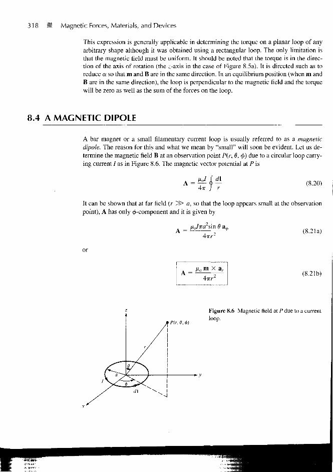
318 Magnetic Forces, Materials, and Devices
This expression is generally applicable in determining the torque on a planar loop of anyarbitrary shape although it was obtained using a rectangular loop. The only limitation isthat the magnetic field must be uniform. It should be noted that the torque is in the direc-tion of the axis of rotation (the z-axis in the case of Figure 8.5a). It is directed such as toreduce a so that m and B are in the same direction. In an equilibrium position (when m andB are in the same direction), the loop is perpendicular to the magnetic field and the torquewill be zero as well as the sum of the forces on the loop.
8.4 A MAGNETIC DIPOLE
A bar magnet or a small filamentary current loop is usually referred to as a magneticdipole. The reason for this and what we mean by "small" will soon be evident. Let us de-termine the magnetic field B at an observation point P(r, 8, 4>) due to a circular loop carry-ing current / as in Figure 8.6. The magnetic vector potential at P is
(8.20)
It can be shown that at far field (r ^> a, so that the loop appears small at the observationpoint), A has only 0-component and it is given by
(8.21a)
or
A
jxj-wa sin
4TIT2
^ o m X
47rr2
ar(8.21b)
P(r, 6, 0)
Figure 8.6 Magnetic field at P due to a currentloop.
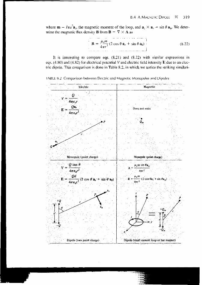
8.4 A MAGNETIC DIPOLE 319
where m = Iira2az, the magnetic moment of the loop, and a, X ar = sin d a0. We deter-mine the magnetic flux density B from B = V X A as
B = ~ : (2 cos 6 ar + sin 6 ; (8.22)
It is interesting to compare eqs. (8.21) and (8.22) with similar expressions ineqs. (4.80) and (4.82) for electrical potential V and electric field intensity E due to an elec-tric dipole. This comparison is done in Table 8.2, in which we notice the striking similari-
TABLE 8.2 Comparison between Electric and Magnetic Monopoles and Dipoles
Electric
V -
Monopoie (point charge)
Qcasd
EQd
(2 cos B ar + sin1©:
+0
Dipole (two point charge)
Magnetic
Does not exist
Qm
Monopoie (point charge)
A = •
sin 0 i 0
4irr2
Me,B = (2 cos Hr + sin 9ae)
47TC3
Dipole (small current loop or bar magnet)

320 Magnetic Forces, Materials, and Devices
Figure 8.7 The B lines due tomagnetic dipoles: (a) a smallcurrent loop with m = IS, (b) abar magnet with m = Qm€.
(a) (b)
ties between B as far field due to a small current loop and E at far field due to an electricdipole. It is therefore reasonable to regard a small current loop as a magnetic dipole. The Blines due to a magnetic dipole are similar to the E lines due to an electric dipole. Figure8.7(a) illustrates the B lines around the magnetic dipole m = IS.
A short permanent magnetic bar, shown in Figure 8.7(b), may also be regarded as amagnetic dipole. Observe that the B lines due to the bar are similar to those due to a smallcurrent loop in Figure 8.7(a).
Consider the bar magnet of Figure 8.8. If Qm is an isolated magnetic charge (polestrength) and € is the length of the bar, the bar has a dipole moment Qm€. (Notice that Qm
does exist; however, it does not exist without an associated — Qm. See Table 8.2.) When thebar is in a uniform magnetic field B, it experiences a torque
T=mXB=2JXB (8.23)
where € points in the direction south-to-north. The torque tends to align the bar with theexternal magnetic field. The force acting on the magnetic charge is given by
F = QmB (8.24)
Since both a small current loop and a bar magnet produce magnetic dipoles, they are equiv-alent if they produce the same torque in a given B field; that is, when
T = QJB = ISB
Hence,
QJ = IS
showing that they must have the same dipole moment.
(8.25)
(8.26)
nsrl«
*~FB
Figure 8.8 A bar magnet in an external magnetic field.

8.4 A MAGNETIC DIPOLE 321
EXAMPLE 8.5Determine the magnetic moment of an electric circuit formed by the triangular loop ofFigure 8.9.
Solution:
From Problem 1.18(c), the equation of a plane is given by Ax + By + Cz + D = 0 whereD= -(A2 + B2 + C2). Since points (2, 0, 0), (0, 2, 0), and (0, 0, 2) lie on the plane, thesepoints must satisfy the equation of the plane, and the constants A, B, C, and D can bedetermined. Doing this gives x + y + z = 2 as the plane on which the loop lies. Thus wecan use
m = ISan
where
S = loop area = - X base X height = - (2 V2)(2 V2)sin 60°
= 4 sin 60°
If we define the plane surface by a function
f(x,y,z) = x + y + z ~ 2 = 0,
V / ^ (a = ±
ay + az)
V 3
We choose the plus sign in view of the direction of the current in the loop (using the right-hand rule, m is directed as in Figure 8.9). Hence
^ (a, + ay + a,)m = 5 (4 sin 60°) r-
V 3= 10(ax + ay + a,) A • m2
Figure 8.9 Triangular loop of Example 8.5.

322 B Magnetic Forces, Materials, and Devices
PRACTICE EXERCISE 8.5
A rectangular coil of area 10 cm2 carrying current of 50 A lies on plane2x + 6y - 3z = 7 such that the magnetic moment of the coil is directed away fromthe origin. Calculate its magnetic moment.
Answer: (1.429a, + 4.286a,, - 2.143az) X 10~2 A • m2
EXAMPLE 8.6A small current loop L, with magnetic moment 53;, A/m is located at the origin whileanother small loop current L2 with magnetic moment 3ay A • m2 is located at (4, —3, 10).Determine the torque on L2.
Solution:
The torque T2 on the loop L2 is due to the field Bj produced by loop L,. Hence,
T2 = m2 X B,
Since m, for loop Lx is along az, we find Bj using eq. (8.22):
B =4irr
(2 cos 9 ar + sin 8 ag)
Using eq. (2.23), we transform m2 from Cartesian to spherical coordinates:
m2 = 3av = 3 (sin 6 sin 4> ar + cos 6 sin 0 ae + cos <t> a^)
At (4, - 3 , 10),
r = V 4 2 + (-3)2 + 102 = 5 V 5
2
V5
Hence,
p 5 1 1tan 6 = — = — = >sin0 = —1=,
z 10 2 V ?COS P =
y - 3 - 3 4t a n <j) = — = > sin 0 = , c o s <j> = —
B_ 4 x X 1 0 ' 7 X 5 / 4 1— j= I j= ar H -j= ae
47T625V5 VV5 V510"7
(4ar + a,)625
m2 - 35V5 5V5 5
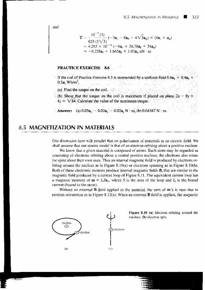
8.5 MAGNETIZATION IN MATERIALS 323
and
T =1 0
4V/5a<A) X (4ar1_ ( 3 a r 6625 (5 V5)
= 4.293 X 10"" (-6a r + 38.78ae + 24a0)= -0.258ar + 1.665a,, + l.O3a0nN • m
PRACTICE EXERCISE 8.6
If the coil of Practice Exercise 8.5 is surrounded by a uniform field 0.6ax + 0.43^ +0.5a. Wb/m2,
(a) Find the torque on the coil.
(b) Show that the torque on the coil is maximum if placed on plane 2x - 8>' +4z = V84. Calculate the value of the maximum torque.
Answer: (a) 0.03a,, - 0.02av - 0.02a. N • m, (b) 0.04387 N • m.
8.5 MAGNETIZATION IN MATERIALS
Our discussion here will parallel that on polarization of materials in an electric field. Weshall assume that our atomic model is that of an electron orbiting about a positive nucleus.
We know that a given material is composed of atoms. Each atom may be regarded asconsisting of electrons orbiting about a central positive nucleus; the electrons also rotate(or spin) about their own axes. Thus an internal magnetic field is produced by electrons or-biting around the nucleus as in Figure 8.10(a) or electrons spinning as in Figure 8.10(b).Both of these electronic motions produce internal magnetic fields B, that are similar to themagnetic field produced by a current loop of Figure 8.11. The equivalent current loop hasa magnetic moment of m = IbSan, where S is the area of the loop and Ib is the boundcurrent (bound to the atom).
Without an external B field applied to the material, the sum of m's is zero due torandom orientation as in Figure 8.12(a). When an external B field is applied, the magnetic
Figure 8.10 (a) Electron orbiting around thenucleus; (b) electron spin.
nucleus
23 electron(J) electron
(a)

324 Magnetic Forces, Materials, and Devices
Figure 8.11 Circular current loop equivalent to electronic motion ofFigure 8.10.
moments of the electrons more or less align themselves with B so that the net magneticmoment is not zero, as illustrated in Figure 8.12(b).
The magnetization M (in amperes/meter) is the magnetic dipole moment per unitvolume.
If there are N atoms in a given volume Av and the kth atom has a magnetic moment m*.,
M = lim k-\
>0 Av(8.27)
A medium for which M is not zero everywhere is said to be magnetized. For a differentialvolume dv', the magnetic moment is dm = M dv'. From eq. (8.21b), the vector magneticpotential due to dm is
dX =X
A-KR1dv' =
According to eq. (7.46),
R
X R-dv'
B = 0, M = 0Hgurc 8.! 2 Magnetic dipole mo-ment in a volume Av: (a) before B isapplied, (b) after B is applied.
(a) (b)

8.5 MAGNETIZATION IN MATERIALS 325
Hence,
Using eq. (7.48) gives
A = — I M X V - dv'4TT R
(8.28)
' - = -V'XM-V'X-
Substituting this into eq. (8.28) yields
4TT Jy, R 4TT JV, fl
Applying the vector identity
V X F dv' = - <J> F X r f S
to the second integral, we obtain
4TT JV, J? 4TT JS , R
Ho f ibdv' JXO(8.29)
4ir )v, R 4TT )S. R
Comparing eq. (8.29) with eqs. (7.42) and (7.43) (upon dropping the primes) gives
h = V X M
and
(8.30)
(8.31)
where Jb is the bound volume current density or magnetization volume current density (inamperes per meter square), Kb is the bound surface current density (in amperes per meter),and an is a unit vector normal to the surface. Equation (8.29) shows that the potential of amagnetic body is due to a volume current density Jb throughout the body and a surfacecurrent Kb on the surface of the body. The vector M is analogous to the polarization P indielectrics and is sometimes called the magnetic polarization density of the medium. Inanother sense, M is analogous to H and they both have the same units. In this respect, asJ = V X H, so is Jb = V X M. Also, Jb and Kb for a magnetized body are similar to ppv
and pps for a polarized body. As is evident in eqs. (8.29) to (8.31), Jh and Kh can be derivedfrom M; therefore, ib and Kb are not commonly used.

326 HI Magnetic Forces, Materials, and Devices
In free space, M = 0 and we have
V X H = it or V XB
(8.32)
where Jy is the free current volume density. In a material medium M i= 0, and as a result,B changes so that
*x(i)-J/+J.-J -= V X H + V X M
or
B = M) (8.33)
The relationship in eq. (8.33) holds for all materials whether they are linear or not. Theconcepts of linearity, isotropy, and homogeneity introduced in Section 5.7 for dielectricmedia equally apply here for magnetic media. For linear materials, M (in A/m) dependslinearly on H such that
(8.34)
where \m is a dimensionless quantity (ratio of M to H) called magnetic susceptibility of themedium. It is more or less a measure of how susceptible (or sensitive) the material is to amagnetic field. Substituting eq. (8.34) into eq. (8.33) yields
B = /xo(l +
or
where
(8.35)
(8.36)
(8.37)
The quantity /x = /io/xr is called the permeability of the material and is measured inhenrys/meter; the henry is the unit of inductance and will be defined a little later. The di-mensionless quantity /xr is the ratio of the permeability of a given material to that of freespace and is known as the relative permeability of the material.
It should be borne in mind that the relationships in eqs. (8.34) to (8.37) hold only forlinear and isotropic materials. If the materials are anisotropic (e.g., crystals), eq. (8.33) stillholds but eqs. (8.34) to (8.37) do not apply. In this case, fi has nine terms (similar to e ineq. 5.37) and, consequently, the fields B, H, and M are no longer parallel.
B
ixr =
- A
1 +
io/xrH
XmE.Mo

8.6 CLASSIFICATION OF MAGNETIC MATERIALS 327
8.6 CLASSIFICATION OF MAGNETIC MATERIALS
In general, we may use the magnetic susceptibility \m or the relative permeability \ir toclassify materials in terms of their magnetic property or behavior. A material is said to benonmagnetic if ym = 0 (or jxr = 1); it is magnetic otherwise^ Free space, air, and materialswith Xm = 0 (or fir = 1) are regar3eTas"fT61imagnetic.
Roughly speaking, magnetic materials may be grouped into three major classes: dia-magnetic, paramagnetic, and ferromagnetic. This rough classification is depicted inFigure 8.13. A material is said to be diamagnetic if it has \xr S 1 (i.e., very small nega-tive Xm)- It is paramagnetic if pr S 1 (i.e., very small positive xm)- If Mr ^ 1 (i-e-> verYlarge positive xm)> the material is ferromagnetic. Table B.3 in Appendix B presents thevalues fir for some materials. From the table, it is apparent that for most practical purposeswe may assume that \ir — 1 for diamagnetic and paramagnetic materials. Thus, we mayregard diamagnetic and paramagnetic materials as linear and nonmagnetic. Ferromagneticmaterials are always nonlinear and magnetic except when their temperatures are abovecurie temperature (to be explained later). The reason for this will become evident as wemore closely examine each of these three types of magnetic materials.
Diamagnetism occurs in materials where the magnetic fields due to electronic motionsof orbiting and spinning completely cancel each other. Thus, the permanent (or intrinsic)magnetic moment of each atom is zero and the materials are weakly affected by a magneticfield. For most diamagnetic materials (e.g., bismuth, lead, copper, silicon, diamond,sodium chloride), xm is of the order of - 1(T5. In certain types of materials called super-conductors at temperatures near absolute zero, "perfect diamagnetism" occurs: xm
= ~ 1or jjir = 0 and B = 0. Thus superconductors cannot contain magnetic fields.2 Except forsuperconductors, diamagnetic materials are seldom used in practice. Although the diamag-netic effect is overshadowed by other stronger effects in some materials, all materialsexhibit diamagnetism.
Materials whose atoms have nonzero permanent magnetic moment may be paramag-netic or ferromagnetic. Paramagnetism occurs in materials where the magnetic fields pro-
Magnetic Materials
Linear
Diamagnetics
Xm<0, M r s 1.0
Paramagnetics
Xm > 0, fir a
Nonlinear
Ferromagnetics
Xm » 0, nr a>
Figure 8.13 Classification of magnetic materials.
2An excellent treatment of superconductors is found in M. A. Plonus, Applied Electromagnetics.New York: McGraw-Hill, 1978, pp. 375-388. Also, the August 1989 issue of the Proceedings ofIEEE is devoted to superconductivity.

328 Magnetic Forces, Materials, and Devices
duced by orbital and spinning electrons do not cancel completely. Unlike diamagnetism,paramagnetism is temperature dependent. For most paramagnetic materials (e.g., air, plat-inum, tungsten, potassium), \m is ofthe order +10~5 to +10~3 and is temperature depen-dent. Such materials find application in masers.
Ferromagnetism occurs in materials whose atoms have relatively large permanentmagnetic moment. They are called ferromagnetic materials because the best knownmember is iron. Other members are cobalt, nickel, and their alloys. Ferromagnetic materi-als are very useful in practice. As distinct from diamagnetic and paramagnetic materials,ferromagnetic materials have the following properties:
1. They are capable of being magnetized very strongly by a magnetic field.2. They retain a considerable amount of their magnetization when removed from the
field.3. They lose their ferromagnetic properties and become linear paramagnetic materials
when the temperature is raised above a certain temperature known as the curie tem-perature. Thus if a permanent magnet is heated above its curie temperature (770°Cfor iron), it loses its magnetization completely.
4. They are nonlinear; that is, the constitutive relation B = /xo/irH does not hold forferromagnetic materials because \x.r depends on B and cannot be represented by asingle value.
Thus, the values of /xr cited in Table B.3 for ferromagnetics are only typical. For example,for nickel \x.r = 50 under some conditions and 600 under other conditions.
As mentioned in Section 5.9 for conductors, ferromagnetic materials, such as iron andsteel, are used for screening (or shielding) to protect sensitive electrical devices from dis-turbances from strong magnetic fields. A typical example of an iron shield is shown inFigure 8.14(a) where the compass is protected. Without the iron shield, the compass givesan erroneous reading due to the effect of the external magnetic field as in Figure 8.14(b).For perfect screening, it is required that the shield have infinite permeability.
Even though B = juo(H + M) holds for all materials including ferromagnetics, therelationship between B and H depends on previous magnetization of a ferromagnetic
Iron shield
(N-»-) *s I)(
(b)
Figure 8.14 Magnetic screening: (a) iron shield protecting a small compass,(b) compass gives erroneous reading without the shield.

8.6 CLASSIFICATION OF MAGNETIC MATERIALS 329
material—its "magnetic history." Instead of having a linear relationship between B and H(i.e., B = fiH), it is only possible to represent the relationship by a magnetization curve orB-H curve.
A typical B-H curve is shown in Figure 8.15. First of all, note the nonlinear relation-ship between B and H. Second, at any point on the curve, fi is given by the ratio B/H andnot by dB/dH, the slope of the curve.
If we assume that the ferromagnetic material whose B-H curve.in Figure 8.15 is ini-tially unmagnetized, as H increases (due to increase in current) from O to maximumapplied field intensity Hm.dX, curve OP is produced. This curve is referred to as the virgin orinitial magnetization curve. After reaching saturation at P, if H is decreased, B does notfollow the initial curve but lags behind H. This phenomenon of B lagging behind H iscalled hysteresis (which means "to lag" in Greek).
If H is reduced to zero, B is not reduced to zero but to Bn which is referred to as thepermanent flux density. The value of Br depends on //max, the maximum applied field in-tensity. The existence of Br is the cause of having permanent magnets. If H increases neg-atively (by reversing the direction of current), B becomes zero when H becomes Hc, whichis known as the coercive field intensity. Materials for which Hc is small are said to be mag-netically hard. The value of Hc also depends on Hmm.
Further increase in H in the negative direction to reach Q and a reverse in its directionto reach P gives a closed curve called a hysteresis loop. The shape of hysteresis loopsvaries from one material to another. Some ferrites, for example, have an almost rectangu-lar hysteresis loop and are used in digital computers as magnetic information storagedevices. The area of a hysteresis loop gives the energy loss (hysteresis loss) per unitvolume during one cycle of the periodic magnetization of the ferromagnetic material. Thisenergy loss is in the form of heat. It is therefore desirable that materials used in electricgenerators, motors, and transformers should have tall but narrow hysteresis loops so thathysteresis losses are minimal.
Initialmagnetizationcurve
Figure 8.15 Typical magnetization (B-H) curve.
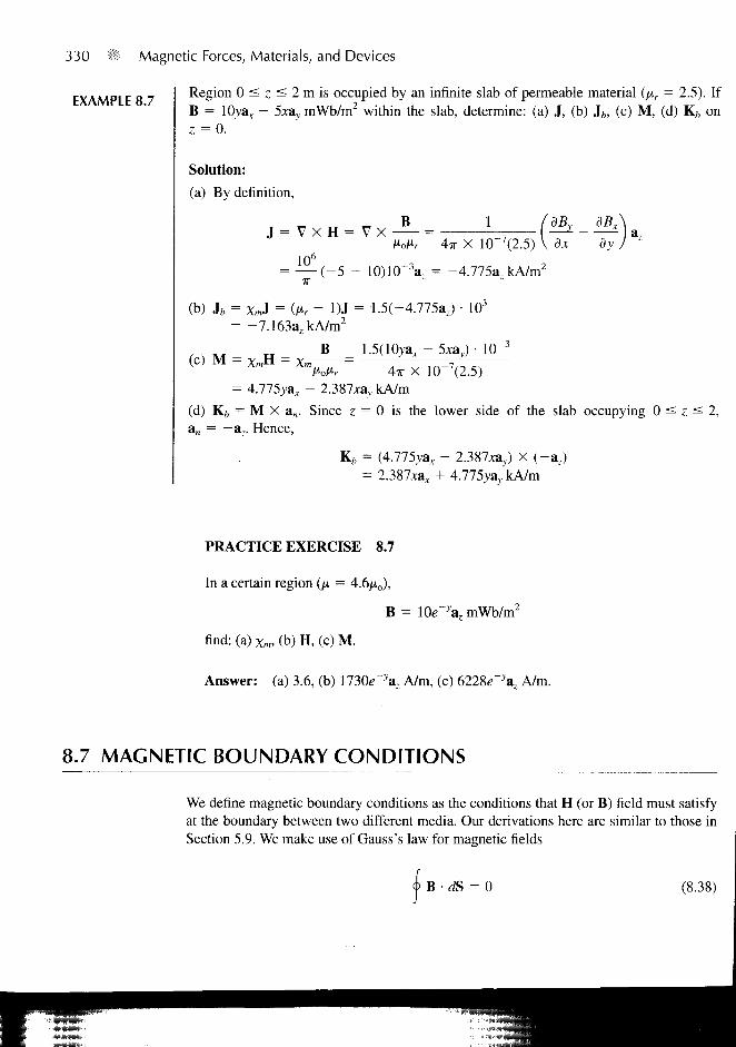
330 Magnetic Forces, Materials, and Devices
EXAMPLE 8.7Region 0 ^ z — 2 m is occupied by an infinite slab of permeable material (/xr = 2.5). IfB = \0y&x — 5xay mWb/m2 within the slab, determine: (a) J, (b) ih, (c) M, (d) Kb onz = 0.
Solution:
(a) By definition,
J = V X H = V X B 1
4ir X 10"'(2.5) V dx dy
dB,a
106
( - 5 - 10)10 X = -4.775azkA/mz
(b) h = XmJ = (Mr - DJ = 1.5(-4.775az) • 103
= -7.163a7kA/m2
(c) M = XmH =B 1.5(10yax - 5xay) • 10
Air X 10"7(2.5)
- 3
= 4.775vax - 2.387xav kA/m(d) Kb = M X an. Since z = 0 is the lower side of the slab occupying 0 < z ^ 2,an = — az. Hence,
Kb = (4.775jax - 2.387xav) X (-a,)= 2.387xax + 4.775jaT'kA/m
PRACTICE EXERCISE 8.7
In a certain region (/i = 4.6/x0),
find: (a) Xm, (b) H, (c) M.
B = We~\ mWb/m2
Answer: (a) 3.6, (b) mOe^a, A/m, (c) 6228e"yaz A/m.
8.7 MAGNETIC BOUNDARY CONDITIONS
We define magnetic boundary conditions as the conditions that H (or B) field must satisfyat the boundary between two different media. Our derivations here are similar to those inSection 5.9. We make use of Gauss's law for magnetic fields
B • dS = 0 (8.38)
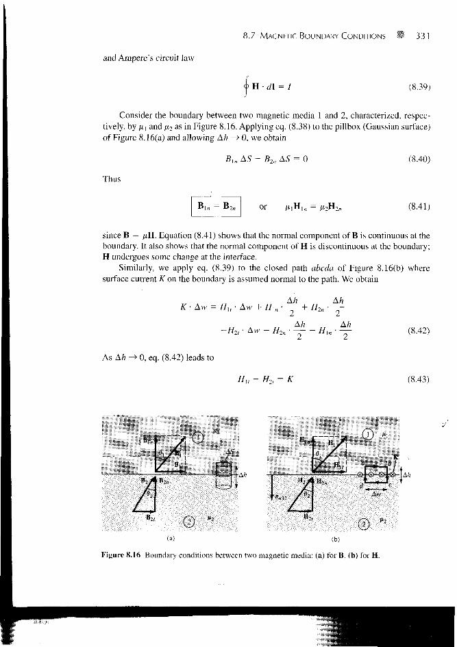
8.7 MAGNETIC BOUNDARY CONDITIONS 331
and Ampere's circuit law
H • d\ = I 3.39)
Consider the boundary between two magnetic media 1 and 2, characterized, respec-tively, by ix{ and /x2 as in Figure 8.16. Applying eq. (8.38) to the pillbox (Gaussian surface)of Figure 8.16(a) and allowing Ah —> 0, we obtain
ln AS - B2n AS = (8.40)
Thus
or (8.41)
since B = ^H. Equation (8.41) shows that the normal component of B is continuous at theboundary. It also shows that the normal component of H is discontinuous at the boundary;H undergoes some change at the interface.
Similarly, we apply eq. (8.39) to the closed path abcda of Figure 8.16(b) wheresurface current K on the boundary is assumed normal to the path. We obtain
Ah\n ' ~~Z I" H2n
Ah
As Ah -> 0, eq. (8.42) leads to
H Aw H M H Ak
Hit H2, — K
(8.42)
(8.43)
fH,
(a) (b)
Figure 8.16 Boundary conditions between two magnetic media: (a) for B, (b) for H.

332 Magnetic Forces, Materials, and Devices
This shows that the tangential component of H is also discontinuous. Equation (8.43) maybe written in terms of B as
— = K (8.44)
In the general case, eq. (8.43) becomes
(H, - H2) X an l2 = K (8.45)
where anl2 is a unit vector normal to the interface and is directed from medium 1 tomedium 2. If the boundary is free of current or the media are not conductors (for K is freecurrent density), K — 0 and eq. (8.43) becomes
I H l r - H2, or (8.46)
Thus the tangential component of H is continuous while that of B is discontinuous at theboundary.
If the fields make an angle 6 with the normal to the interface, eq. (8.41) results in
cos 0[ = Bln = B2n = B2 cos
while eq. (8.46) produces
Mi
B2
sin 0, = Hu = H2t = — sin 62
(8.47)
(8.48)
Dividing eq. (8.48) by eq. (8.47) gives
r tan I
tan02(8.49)
which is [similar to eq. (5.65)] the law of refraction for magnetic flux lines at a boundarywith no surface current.
EXAMPLE 8.8 Given that H! = -2a x + 6ay + 4az A/m in region y - x - 2 < 0 where /*] = 5/*0, cal-culate
(a) M, and B,
(b) H2 and B2 in region y - x - 2 > 0 where ju2 = 2;ito
Solution:
Since j - x - 2 = 0 i s a plane, y - x < 2 o r y < x + 2 i s region 1 in Figure 8.17. Apoint in this region may be used to confirm this. For example, the origin (0, 0) is in this

8.7 MAGNETIC BOUNDARY CONDITIONS ;- 333
Figure 8.17 For Example 8.8.
region since 0 - 0 - 2 < 0. If we let the surface of the plane be described by j{x, y) =y — x — 2, a unit vector normal to the plane is given by
(a) M,
= ay - a*
V~2= ( / M - 1)H, = ( 5 - lX-2 ,6 ,4 )
+ 24av, + 16a7 A/m
(b) HlB = (H! • aB)aB = | ( -2 ,6 ,4)
B, = ^JHJ = Aio/nnH, = 4TT X 10"7(5)(-2, 6,4)= -12.57a* + 37.7ay + 25.13a,/iWb/m2
( -1 ,1 ,0)1 ( -1 ,1 ,0)
Vl J V2
But
Hence,
— Hln + Hlf
Ult = H, - Hln = (-2, 6, 4) - (-4,4, 0)= 2ar + 2av + 4a7
Using the boundary conditions, we have
H2, = H u = 4az
or
H2n = — HIB = | ( -4a , + 4ay) = -10a* + 10a,
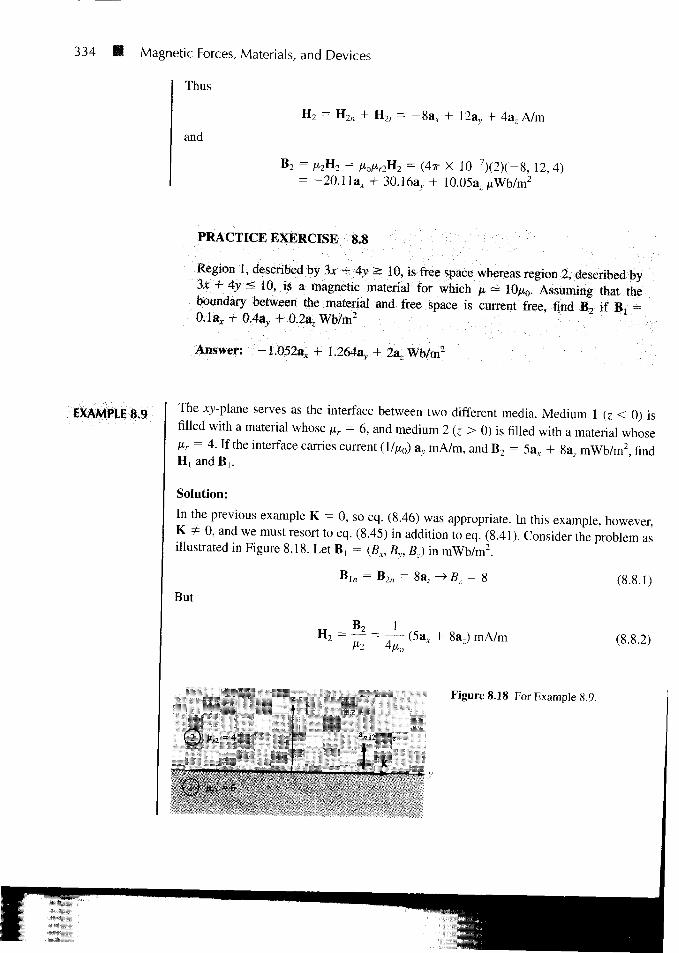
334 f i Magnetic Forces, Materials, and Devices
Thus
H 2 = H2n + H2, = - 8 a x + 12av + 4a. A/m
and
B 2 = fi2H2 = jxojxr2n2 = (4TT X 10 7 ) (2 ) ( -8 , 12, 4)= -20 .11a , + 30.16ay + 10.05a.
PRACTICE EXERCISE 8.8
Region 1, described by 3x + Ay > 10, is free space whereas region 2, described by3x + Ay < 10, is a magnetic material for which /* = J OJU0. Assuming that theboundary between the material and free space is current free find B7 if B, =0.1a,+ 0.4av +0.2a. Wb/m2
Answer: -1.052a, + 1.264a,. + 2az Wb/m2
EXAMPLE 8.9 The xy-plane serves as the interface between two different media. Medium 1 (z < 0) isfilled with a material whose Mr = 6, and medium 2 (z > 0) is filled with a material whoseHr = 4. If the interface carries current (1/Mo) av mA/m, and B2 = 5a, + 8a mWb/m2 findHiandB,.
Solution:
In the previous example K = 0, so eq. (8.46) was appropriate. In this example, however,K # 0, and we must resort to eq. (8.45) in addition to eq. (8.41). Consider the problem asillustrated in Figure 8.18. Let B, = (Bx, By, Bz) in mWb/m2.
But
[2) nr2=4
Bin = B2 n
(5a,
K-» -y
B7 = 8
mA/m
Figure 8.18 For Example 8.9.
(8.8.1)
(8.8.2)

8.7 MAGNETIC BOUNDARY CONDITIONS *> 335
and
H, =B, 1
{Bxax + Byay + Bzaz) mA/m (8.8.3)
Having found the normal components, we can find the tangential components using
(H, - H2) X anl2 = K
or
H, X anl2 = H2 X aBl2 + K (8.8.4)
Substituting eqs. (8.8.2) and (8.8.3) into eq. (8.8.4) gives
— ( B A + 5vay + Bzaz) X az = —- (5a, + 8az) X a, + — av6^ ' 4/x M
Equating components yields
By = 0, :
From eqs. (8.8.1) and (8.8.5),
- 54
o r
6T4
B, = 1.5a,, + 8azmWb/m2
H, = — = — (0.25ax + 1.33a,) mA/mMl Mo
and
(8.8.5)
H2 = — (1.25a* + 2az) mA/mMo
Note that Hlx is (1//O mA/m less than H2x due to the current sheet and also thatBin = B2n.
PRACTICE EXERCISE 8.9
A unit normal vector from region 2 {ft, = 2MO) to region 1 {ft, = Mo) is a«2i =
(6ax + 2a, - 3az)/7. If H, = \0ax + ay + 12az A/m and H2 =4az A/m, determine
(a) H ^
(b) The surface current density K on the interface
(c) The angles Bj and B2 make with the normal to the interface.
- 5ay +
Answer: (a) 5.833, (b) 4.86a* - 8.64a. + 3.95a, A/m, (c)76.27°, 77.62°.

336 Magnetic Forces, Materials, and Devices
8.8 INDUCTORS AND INDUCTANCES
A circuit (or closed conducting path) carrying current / produces a magnetic field B whichcauses a flux ¥* = J B • dS to pass through each turn of the circuit as shown in Figure 8.19.If the circuit has N identical turns, we define the flux linkage X as
X = NY (8.50)
Also, if the medium surrounding the circuit is linear, the flux linkage X is proportional tothe current / producing it; that is,
or X = (8.51)
where Lisa constant of proportionality called the inductance of the circuit. The inductanceL is a property of the physical arrangement of the circuit. A circuit or part of a circuit thathas inductance is called an inductor. From eqs. (8.50) and (8.51), we may define induc-tance L of an inductor as the ratio of the magnetic flux linkage X to the current / through theinductor; that is,
X(8.52)
The unit of inductance is the henry (H) which is the same as webers/ampere. Since thehenry is a fairly large unit, inductances are usually expressed in millihenrys (mH).
The inductance denned by eq. (8.52) is commonly referred to as self-inductance sincethe linkages are produced by the inductor itself. Like capacitances, we may regard induc-tance as a measure of how much magnetic energy is stored in an inductor. The magneticenergy (in joules) stored in an inductor is expressed in circuit theory as:
Wm = ^L (8.53)
Figure 8.19 Magnetic field B produced by a circuit.

8.8 INDUCTORS AND INDUCTANCES 337
or
L — — (8.54)
Thus the self-inductance of a circuit may be defined or calculated from energy considera-tions.
If instead of having a single circuit we have two circuits carrying current I\ and I2 asshown in Figure 8.20, a magnetic interaction exists between the circuits. Four componentfluxes ^ n , f|2, V 21, and f22
a r e produced. The flux "f \2, for example, is the flux passingthrough circuit 1 due to current I2 in circuit 2. If B2 in the field due to I2 and S\ is the areaof circuit 1, then
(8.55)
We define the mutual inductance Mn as the ratio of the flux linkage X12 = N{fu on circuit1 to current I2, that is,
! .. x1212 = T =
I i
(8.56)
Similarly, the mutual inductance M2\ is defined as the flux linkages of circuit 2 per unitcurrent /,; that is,
M7I =h /,
(8.57a)
It can be shown by using energy concepts that if the medium surrounding the circuits islinear (i.e., in the absence of ferromagnetic material),
M12 = M2{ (8.57b)
The mutual inductance Mi2 or M2l is expressed in henrys and should not be confused withthe magnetization vector M expressed in amperes/meter.
Figure 8.20 Magnetic interaction betweentwo circuits.

338 B Magnetic Forces, Materials, and Devices
We define the self-inductance of circuits 1 and 2, respectively, as
L = x,, _ w(8.58)
and
U = x,22 (8.59)
where V, = + + ¥^2-The total energy in the magnetic field is thesum of the energies due to Lh L2, andMI2 (orM21); that is,
Wm = W2 + W12
2 + ~L2I22 (8.60)
The positive sign is taken if currents /] and I2 flow such that the magnetic fields of the twocircuits strengthen each other. If the currents flow such that their magnetic fields opposeeach other, the negative sign is taken.
As mentioned earlier, an inductor is a conductor arranged in a shape appropriate tostore magnetic energy. Typical examples of inductors are toroids, solenoids, coaxial trans-mission lines, and parallel-wire transmission lines. The inductance of each of these induc-tors can be determined by following a procedure similar to that taken in determining thecapacitance of a capacitor. For a given inductor, we find the self-inductance L by takingthese steps:
1. Choose a suitable coordinate system.2. Let the inductor carry current /.3. Determine B from Biot-Savart's law (or from Ampere's law if symmetry exists)
and calculate f from V = / B • dS.X NY
4. Finally find L from L = — = .
The mutual inductance between two circuits may be calculated by taking a similar proce-dure.
In an inductor such as a coaxial or a parallel-wire transmission line, the inductanceproduced by the flux internal to the conductor is called the internal inductance L-m whilethat produced by the flux external to it is called external inductance Lext. The total induc-tance L is
Mn ' ^e\l
Just as it was shown that for capacitors
eRC = -
a
(8.61)
(6.35)

it can be shown that
LexlC =
8.9 MAGNETIC ENERGY -.-> 339
(8.62)
Thus Lext may be calculated using eq. (8.62) if C is known.A collection of formulas for some fundamental circuit elements is presented in Table
8.3. All formulas can be derived by taking the steps outlined above.3
8.9 MAGNETIC ENERGY
Just as the potential energy in an electrostatic field was derived as
eE dvWE = - D • E dv = ~ (4.96)
we would like to derive a similar expression for the energy in a magnetostatic field. Asimple approach is using the magnetic energy in the field of an inductor. From eq. (8.53),
(8.53)
The energy is stored in the magnetic field B of the inductor. We would like to expresseq. (8.53) in terms of B or H.
Consider a differential volume in a magnetic field as shown in Figure 8.21. Let thevolume be covered with conducting sheets at the top and bottom surfaces with current A/.
conductingsheets
Figure 8.21 A differential volumein a magnetic field.
'Additional formulas can be found in standard electrical handbooks or in H. Knoepfel, Pulsed HighMagnetic Fields. Amsterdam: North-Holland, 1970, pp. 312-324.

o
TABLE 8.3 A Collection of Formulas for Inductance of Common Elements
1. Wire
L
L =877
2.
3.
Hollow
L = —2TI
€»a
Parallel
L = —-IT
cylinder
' \ a
wires
f J- l n -
(3
4. Coaxial conductor
L = In -7T a
5. Circular loop
ii ^ 1 In — — 22TT \ d
€ = 27rpo, po » d
6. Solenoid
L =
7. Torus (of circular cross section)
L = voN2[Po - Vp2
o - a2]2.1
8. Sheet
L = /to 2€ /«
8.9 MAGNETIC ENERGY 341
We assume that the whole region is filled with such differential volumes. From eq. (8.52),each volume has an inductance
AL =AT tiHAxAz
A/ A/
where A/ = H Ay. Substituting eq. (8.63) into eq. (8.53), we have
AWm = -AL A/2 = - iiH2 Ax Ay Az
or
_ l 2m j
The magnetostatic energy density wm (in J/m3) is defined as
AWm 1 .. ,wm = lim
Av->0 Av
Hence,
1 , 1 B2
2 2 2/*
Thus the energy in a magnetostatic field in a linear medium is
Wm= wmdv
or
which is similar to eq. (4.96) for an electrostatic field.
(8.63)
(8.64)
(8.65)
(8.66)
EXAMPLE 8.10Calculate the self-inductance per unit length of an infinitely long solenoid.
Solution:
We recall from Example 7.4 that for an infinitely long solenoid, the magnetic flux insidethe solenoid per unit length is
B = nH = uln

342 Magnetic Forces, Materials, and Devices
where n = N/€ = number of turns per unit length. If S is the cross-sectional area of the so-lenoid, the total flux through the cross section is
Y = BS =
Since this flux is only for a unit length of the solenoid, the linkage per unit length is
X' = - = nV = im2IS
and thus the inductance per unit length is
L X' ,
V = /xn2S H/m
PRACTICE EXERCISE 8.10
A very long solenoid with 2 X 2 cm cross section has an iron core (p,r - 1000) and4000 turns/meter. If it carries a current of 500 mA, find
(a) Its self-inductance per meter
(b) The energy per meter stored in its field
Answer: (a) 8.042 H/m, (b) 1.005 J/m.
EXAMPLE 8.11 Determine the self-inductance of a coaxial cable of inner radius a and outer radius b.
Solution:
The self-inductance of the inductor can be found in two different ways: by taking the foursteps given in Section 8.8 or by using eqs. (8.54) and (8.66).
Method 1: Consider the cross section of the cable as shown in Figure 8.22. We recallfrom eq. (7.29) that by applying Ampere's circuit law, we obtained for region1 (0 < p < a),
and for region 2 (a < p < b),
B , - - j a<*2-wa

8.9 MAGNETIC ENERGY 343
© z-axis
(a) (b)
Figure 8.22 Cross section of the coaxial cable: (a) for region 1,0 < p < a, (b) for region 2, a < p < b; for Example 8.11.
We first find the internal inductance Lin by considering the flux linkages due to the innerconductor. From Figure 8.22(a), the flux leaving a differential shell of thickness dp is
dYi = 5, dp dz = - ~ dp dz2ira
The flux linkage is dxPl multiplied by the ratio of the area within the path enclosing the fluxto the total area, that is,
because / is uniformly distributed over the cross section for d.c. excitation. Thus, the totalflux linkages within the differential flux element are
flip dp dz
lira2 a2
For length € of the cable,
X, = r dp dz8TT
/ 8TT
The internal inductance per unit length, given by
m i H/m
(8.11.1)
(8.11.2)
is independent of the radius of the conductor or wire. Thus eqs. (8.11.1) and (8.11.2) are alsoapplicable to finding the inductance of any infinitely long straight conductor of finite radius.

344 Magnetic Forces, Materials, and Devices
We now determine the external inductance Lext by considering the flux linkagesbetween the inner and the outer conductor as in Figure 8.22(b). For a differential shell ofthickness dp,
df2 = B2 dp dz2-Kp
dp dz
In this case, the total current / is enclosed within the path enclosing the flux. Hence,
X, =p=a Jz=0
al dp dz i"/€ , b= In —
2irp 2-K a
_ \ 2 _ ^ bL e x t ~ I ~ 2* a
Thus
\
or the inductance per length is
H/m
Method 2: It is easier to use eqs. (8.54) and (8.66) to determine L, that is,
2W
where
or L =
1 f B1
I H dv = —dv2
Hence
2 [B\ 2T2 2
— — p dp d(j) dz4TT a
= - ^ - r dz dct> p 3 dp =0 J0 J0
8TT
^ P 6?P d<t> dz

8.9 MAGNETIC ENERGY • 345
and
as obtained previously.
PRACTICE EXERCISE 8.11
Calculate the self-inductance of the coaxial cable of Example 8.11 if the inner con-ductor is made of an inhomogeneous material having a = 2aJ{\ + p).
aot uj \ b (1 + b)Answer: 1 In In
8TT IT I a (1 + a)
EXAMPLE 8.12 Determine the inductance per unit length of a two-wire transmission line with separationdistance d. Each wire has radius a as shown in Figure 6.37.
Solution:
We use the two methods of the last example.
Method 1: We determine Lin just as we did in the last example. Thus for region0<p<a,we obtain
_ alt
as in the last example. For region a < p < d - a, the flux linkages between the wires arecd—a /*€ T rt) jX2 =
The flux linkages produced by wire 1 are
dp dz = —- In2TT a
X, + \? =alt alt d- a
1 In8TT 2TT a
By symmetry, the same amount of flux produced by current —/ in wire 2. Hence the totallinkages are
X 2(Xi+X2) [If d 5s> a, the self-inductance per unit length is
H/m

346 11 Magnetic Forces, Materials, and Devices
Method 2: From the last example,
Lm ~ 8
Now
B2dv 1 {[[ ii2!2
L e x t I2) 2» l \
dz
^ p dp d(j) dz
d—a
2ir a
Since the two wires are symmetrical,
L = 2 (Lin + Lext)
as obtained previously.
PRACTICE EXERCISE 8.12
Two #10 copper wires (2.588 mm in diameter) are placed parallel in air with a sepa-ration distance d between them. If the inductance of each wire is 1.2 jiiH/m, calculate
(a) Lin and Lext per meter for each wire
(b) The separation distance d
Answer: (a) 0.05,1.15 juH/m, (b) 40.79 cm.
EXAMPLE 8.13Two coaxial circular wires of radii a and b(b > a) are separated by distance h(h ^> a, b)as shown in Figure 8.23. Find the mutual inductance between the wires.
Solution:
Let current /, flow in wire 1. At an arbitrary point P on wire 2, the magnetic vector poten-tial due to wire 1 is given by eq. (8.21a), namely
A , =A[h2 + b2f2
If/i » b
b

8.10 MAGNETIC CIRCUITS 347
Figure 8.23 Two coaxial circular wires; for Example8.13.
Hence,
and
u;,21.2
• d\2 =4/r'
/x7r/,a b
~2h3
lbl
PRACTICE EXERCISE 8.13
Find the mutual inductance of two coplanar concentric circular loops of radii 2 mand 3 m.
Answer: 2.632 /*H.
8.10 MAGNETIC CIRCUITS
The concept of magnetic circuits is based on solving some magnetic field problems usingcircuit approach. Magnetic devices such as toroids, transformers, motors, generators, andrelays may be considered as magnetic circuits. The analysis of such circuits is made simpleif an analogy between magnetic circuits and electric circuits is exploited. Once this is done,we can directly apply concepts in electric circuits to solve their analogous magnetic circuits.
The analogy between magnetic and electric circuits is summarized in Table 8.4 andportrayed in Figure 8.24. The reader is advised to pause and study Table 8.4 and Figure8.24. First, we notice from the table that two terms are new. We define the magnetomotiveforce (mmf) 9* (in ampere-turns) as
(8.67)

348 Magnetic Forces, Materials, and Devices
TABLE 8.4 Analogy between Electric and MagneticCircuits
Electric
Conductivity a
Field intensity E
Current / = / J • dS
Current density J = — = oE
Electromotive force (emf) VResistance R
Conductance G = —R
V (Ohm's law R = — = —
or V = E( = IR
Kirchoff's laws:E / = 0
J. V - 2 RI = 0
Magnetic
Permeability /j
Field intensity H
Magnetic flux V = / B • dS
Flux density B = — = fiH
Magnetomotive force (mmf) 9Reluctance 2ft
Permeance 9* = —gft
Ohm's law gft = — = —
or 9 = Hi = » = Nl
Kirchhoff's laws:
The source of mmf in magnetic circuits is usually a coil carrying current as in Figure 8.24.We also define reluctance 2ft (in ampere-turns/weber) as
(8.68)
where € and S are, respectively, the mean length and the cross-sectional area of the mag-netic core. The reciprocal of reluctance is permeance (3>. The basic relationship for circuitelements is Ohm's law (V = IR):
(8.69)
Based on this, Kirchhoff's current and voltage laws can be applied to nodes and loops of agiven magnetic circuit just as in an electric circuit. The rules of adding voltages and for
Figure 8.24 Analogy between(a) an electric circuit, and (b) amagnetic circuit.
(a) (b)

8.11 FORCE ON MAGNETIC MATERIALS 349
combining series and parallel resistances also hold for mmfs and reluctances. Thus for nmagnetic circuit elements in series
and
3? = 3%,
For n magnetic circuit elements in parallel,
and
(8.70)
(8.71)
(8.72)
(8.73)
Some differences between electric and magnetic circuits should be pointed out. Unlikean electric circuit where current / flows, magnetic flux does not flow. Also, conductivity ais independent of current density J in an electric circuit whereas permeability JX varies withflux density B in a magnetic circuit. This is because ferromagnetic (nonlinear) materialsare normally used in most practical magnetic devices. These differences notwithstanding,the magnetic circuit concept serves as an approximate analysis of practical magneticdevices.
8.11 FORCE ON MAGNETIC MATERIALS
It is of practical interest to determine the force that a magnetic field exerts on a piece ofmagnetic material in the field. This is useful in electromechanical systems such as electro-magnets, relays, rotating machines, and magnetic levitation. Consider, for example, anelectromagnet made of iron of constant relative permeability as shown in Figure 8.25. Thecoil has N turns and carries a current /. If we ignore fringing, the magnetic field in the airgap is the same as that in iron (Bln = B2n). To find the force between the two pieces of iron,we calculate the change in the total energy that would result were the two pieces of themagnetic circuit separated by a differential displacement d\. The work required to effect
dlA
Figure 8.25 An electromagnet.
/2F
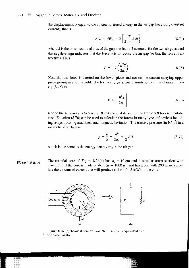
350 Magnetic Forces, Materials, and Devices
the displacement is equal to the change in stored energy in the air gap (assuming constantcurrent), that is
1 B-Fdl = dWm = 2 | Sdl
2 Mo(8.74)
where S is the cross-sectional area of the gap, the factor 2 accounts for the two air gaps, andthe negative sign indicates that the force acts to reduce the air gap (or that the force is at-tractive). Thus
F = -2B2S
(8.75)
Note that the force is exerted on the lower piece and not on the current-carrying upperpiece giving rise to the field. The tractive force across a single gap can be obtained fromeq. (8.75) as
F = -B2S
(8.76)
Notice the similarity between eq. (8.76) and that derived in Example 5.8 for electrostaticcase. Equation (8.76) can be used to calculate the forces in many types of devices includ-ing relays, rotating machines, and magnetic levitation. The tractive pressure (in N/m2) in amagnetized surface is
PF
S
B1
(8.77)
which is the same as the energy density wm in the air gap.
EXAMPLE 8.14The toroidal core of Figure 8.26(a) has po = 10 cm and a circular cross section witha = 1 cm. If the core is made of steel (/x = 1000 /io) and has a coil with 200 turns, calcu-late the amount of current that will produce a flux of 0.5 mWb in the core.
(a) (b)
Figure 8.26 (a) Toroidal core of Example 8.14; (b) its equivalent elec-tric circuit analog.
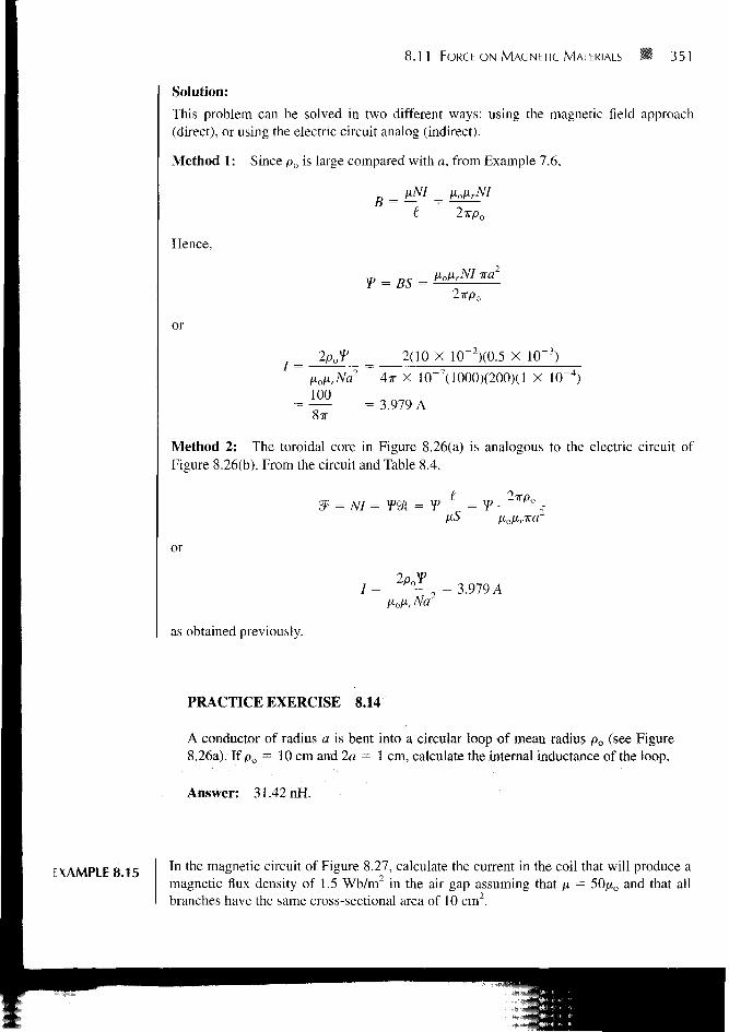
8.11 FORCE ON MAGNETIC MATERIALS 351
Solution:
This problem can be solved in two different ways: using the magnetic field approach(direct), or using the electric circuit analog (indirect).
Method 1: Since p0 is large compared with a, from Example 7.6,
UNI _ floHrNI
Hence,
B =
= BS =HolirNI tea
2TTP0
or
8TT
_ 2(10 X 10~2)(0.5 X 10~3)
~ 4TT X 10~7(1000)(200)(l X 10
= 3.979 A
Method 2: The toroidal core in Figure 8.26(a) is analogous to the electric circuit ofFigure 8.26(b). From the circuit and Table 8.4.
or
/ = = 3.979 A
as obtained previously.
PRACTICE EXERCISE 8.14
A conductor of radius a is bent into a circular loop of mean radius po (see Figure8.26a). If p0 = 10 cm and 2a - 1 cm, calculate the internal inductance of the loop.
Answer: 31.42 nH.
EXAMPLE 8.15 In the magnetic circuit of Figure 8.27, calculate the current in the coil that will produce amagnetic flux density of 1.5 Wb/m in the air gap assuming that fi = 50/xo and that allbranches have the same cross-sectional area of 10 cm2.
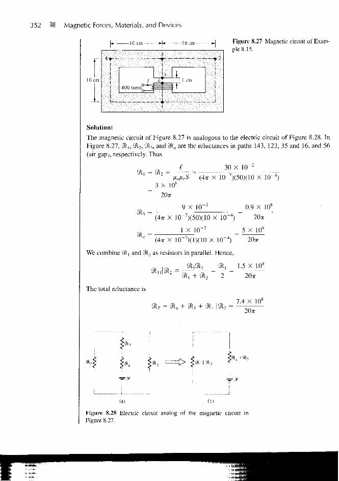
352 =* Magnetic Forces, Materials, and Devices
Figure 8.27 Magnetic circuit of Exam-ple 8.15.
10 cm
Solution:
The magnetic circuit of Figure 8.27 is analogous to the electric circuit of Figure 8.28. InFigure 8.27, Sft,, 2ft2, 2/l3, and <3la are the reluctances in paths 143, 123, 35 and 16, and 56(air gap), respectively. Thus
(3i,='3i7 =
3 X 10s
30 X 10~z
(4TT X 10 7)(50)(10 X
20TT
9 X 10"3 (4TT X 10~7)(50)(10 X
1 X 10~2
0.9 X 10s
20TT
5 X 10,8
'J"a ~ (4,r x 10"7)(l)(10 X 10~4) ~ 20ir
We combine 91, and 9l2 as resistors in parallel. Hence,
„ ,,„ 2ft,2ft7 2/1, 1.5 X 10⁸
The total reluctance is
20x
7.4 X 108
91,
(a) (b)
Figure 8.28 Electric circuit analog of the magnetic circuit inFigure 8.27.

8.11 FORCE ON MAGNETIC MATERIALS 353
The
But
mmf is
r.-r = BaS. Hence
i a
1 —
= 44
52ft
N.16
T
A
= NI = YJ
1.5 X 10 X 10~4 X 7.4 X 108
400 X 20TT
PRACTICE EXERCISE 8.15
The toroid of Figure 8.26(a) has a coil of 1000 turns wound on its core. Ifp 0 = 10 cm and a = 1 cm, what current is required to establish a magnetic flux of0.5 mWb
(a) If the core is nonmagnetic
(b) If the core has /xr = 500
Answer: (a) 795.8 A, (b) 1.592 A.
EXAMPLE 8.16 A U-shaped electromagnet shown in Figure 8.29 is designed to lift a 400-kg mass (whichincludes the mass of the keeper). The iron yoke (jxr = 3000) has a cross section of 40 cm2
and mean length of 50 cm, and the air gaps are each 0.1 mm long. Neglecting the reluc-tance of the keeper, calculate the number of turns in the coil when the excitation currentis 1 A.
Solution:
The tractive force across the two air gaps must balance the weight. Hence
F = 2(B2
aS)= mg
NI Figure 8.29 U-shaped electromagnet; for Example 8.16.
- iron yoke
- keeper
' weisht

354 Magnetic Forces, Materials, and Devices
or
But
Since
mgno _ 400 X 9.8 X 4TT X 10 - i
S 40 X
Bn = 1.11 Wb/m2
cm = ZJL =ta 2 X 0.1 10- 3 10b
Air X 10 7 X 40 X 10 4
50 X 10~2
48TT
4TT X 10"' X 3000 X 40 X 10~
3? = NI = —NI6 + 5 11
5 X 10"
48TT
P-o
11 L
7V= 162
11 X 1.11 X 0.1 X 10
6 X 4TT X 10~7 X 1
PRACTICE EXERCISE 8.16
Find the force across the air gap of the magnetic circuit of Example 8.15.
Answer: 895.2 N.
SUMMARY 1. The Lorentz force equation
F = g(E + u X B) = mdudt
relates the force acting on a particle with charge Q in the presence of EM fields. It ex-presses the fundamental law relating EM to mechanics.
2. Based on the Lorentz force law, the force experienced by a current element Idl in amagnetic field B is
dV = Idl X B
From this, the magnetic field B is defined as the force per unit current element.

SUMMARY • 355
3. The torque on a current loop with magnetic moment m in a uniform magnetic field B is
T = m X B = ISan X B
4. A magnetic dipole is a bar magnet or a small filamental current loop; it is so called dueto the fact that its B field lines are similar to the E field lines of an electric dipole.
5. When a material is subjected to a magnetic field, it becomes magnetized. The magne-tization M is the magnetic dipole moment per unit volume of the material. For linearmaterial,
where \m is the magnetic susceptibility of the material.6. In terms of their magnetic properties, materials are either linear (diamagnetic or para-
magnetic) or nonlinear (ferromagnetic). For linear materials,
B = ,xH = = /xo(l + + M)
where /x = permeability and \xr = \il\xo = relative permeability of the material. Fornonlinear material, B = fi(H) H, that is, JX does not have a fixed value; the relationshipbetween B and H is usually represented by a magnetization curve.
7. The boundary conditions that H or B must satisfy at the interface between two differ-ent media are
(H, - H2) X anl2 = K or Hu = H2/ if K = 0
where anl2 is a unit vector directed from medium 1 to medium 2.8. Energy in a magnetostatic field is given by
Wm = - | B Udv
For an inductor carrying current /
= Vm 2
Thus the inductance L can be found using
L =B -Hdv
9. The inductance L of an inductor can also be determined from its basic definition: theratio of the magnetic flux linkage to the current through the inductor, that is,
_ X NY~ I ~ I

356 II Magnetic Forces, Materials, and Devices
Thus by assuming current /, we determine B and !P = / B • dS, and finally find
L = NY/I.10. A magnetic circuit can be analyzed in the same way as an electric circuit. We simply
keep in mind the similarity between
= NI= 4> H = TO and V= IR
that is,
Thus we can apply Ohms and Kirchhoff's laws to magnetic circuits just as we applythem to electric circuits.
11. The magnetic pressure (or force per unit surface area) on a piece of magnetic material is
F 1~ = ~S 2
B2
—2/xo
where B is the magnetic field at the surface of the material.
8.1 Which of the following statements are not true about electric force Fe and magnetic forceFm on a charged particle?
(a) E and Fc are parallel to each other whereas B and Fm are perpendicular to each other.
(b) Both Fe and Fm depend on the velocity of the charged particle.
(c) Both Fe and ¥m can perform work.
(d) Both Fc and Fm are produced when a charged particle moves at a constant velocity.
(e) Fm is generally small in magnitude compared to Fe.
(f) Fe is an accelerating force whereas Fm is a purely deflecting force.
8.2 Two thin parallel wires carry currents along the same direction. The force experienced byone due to the other is
(a) Parallel to the lines
(b) Perpendicular to the lines and attractive
(c) Perpendicular to the lines and repulsive
(d) Zero
8.3 The force on differential length d\ at point P in the conducting circular loop in Figure8.30 is
(a) Outward along OP
(b) Inward along OP

o
o
o
o
© B
o
REVIEW QUESTIONS #i 357
Q Figure 8.30 For Review Questions 8.3 and 8.4.
O
O
O
(c) In the direction of the magnetic field
(d) Tangential to the loop at P
8.4 The resultant force on the circular loop in Figure 8.30 has the magnitude of
(a) 2wpJB
(b) irpllB
(c) 2PJB
(d) Zero
8.5 What is the unit of magnetic charge?
(a) Ampere-meter square
(b) Coulomb
(c) Ampere
(d) Ampere-meter
8.6 Which of these materials requires the least value of magnetic field strength to magne-tize it?
(a) Nickel
(b) Silver
(c) Tungsten
(d) Sodium chloride
8.7 Identify the statement that is not true of ferromagnetic materials.
(a) They have a large \m.
(b) They have a fixed value of fir.
(c) Energy loss is proportional to the area of the hysteresis loop.
(d) They lose their nonlinearity property above the curie temperature.

358 B Magnetic Forces, Materials, and Devices
8.8 Which of these formulas is wrong?
(a) Bu,= B2n
(b) B2 = Vfi2,, + B\,
(c) // , = //„, + Hu
(d) a,,2i X (H t — H2) = K, where an2i is a unit vector normal to the interface and di-rected from region 2 to region 1.
8.9 Each of the following pairs consists of an electric circuit term and the corresponding mag-netic circuit term. Which pairs are not corresponding?
(a) V and S5
(b) GandSP
(c) e and n
(d) IR and tf9l
(e) 2 / = 0 and 2 f = 0
8.10 A multilayer coil of 2000 turns of fine wire is 20 mm long and has a thickness 5 mm ofwinding. If the coil carries a current of 5 mA, the mmf generated is
(a) lOA-t
(b) 500 A-t
(c) 2000 A-t
(d) None of the above
Answers: 8.1 b,c, 8.2b, 8.3a, 8.4d, 8.5d, 8.6a, 8.7b, 8.8c, 8.9c,d, 8.10a.
PROBLEMS• 8.1 An electron with velocity u = (3ar + 12aY — 4az) X 105m/s experiences no net
J force at a point in a magnetic field B = Wax + 20av + 30a;. mWb/m2. Find E at thatpoint.
8.2 A charged particle of mass 1 kg and charge 2 C starts at the origin with velocity 10az m/sin a magnetic field B = 1 a, Wb/m2. Find the location and the kinetic energy of the parti-cle at t = 2 s.
*8.3 A particle with mass 1 kg and charge 2 C starts from rest at point (2, 3, - 4 ) in a regionwhere E = - 4 a v V/m and B = 5ar Wb/m2. Calculate
(a) The location of the particle at t = I s
(b) Its velocity and K.E. at that location
8.4 A — 2-mC charge starts at point (0, 1, 2) with a velocity of 5ax m/s in a magnetic fieldB = 6av Wb/m . Determine the position and velocity of the particle after 10 s assumingthat the mass of the charge is 1 gram. Describe the motion of the charge.
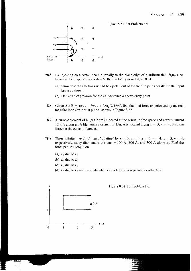
PROBtEMS ; i 359
Figure 8.31 For Problem 8.5.
*8.5 By injecting an electron beam normally to the plane edge of a uniform field Boaz, elec-trons can be dispersed according to their velocity as in Figure 8.31.
(a) Show that the electrons would be ejected out of the field in paths parallel to the input
beam as shown.
(b) Derive an expression for the exit distance d above entry point.
8.6 Given that B = 6xa^ — 9yay + 3zaz Wb/m2, find the total force experienced by the rec-tangular loop (on z = 0 plane) shown in Figure 8.32.
8.7 A current element of length 2 cm is located at the origin in free space and carries current12 mA along ax. A filamentary current of 15az A is located along x = 3, y = 4. Find theforce on the current filament.
*8.8 Three infinite lines L b L2, and L3 defined by x = 0, y = 0; x = 0, y = 4; x = 3, y = 4,respectively, carry filamentary currents —100 A, 200 A, and 300 A along az. Find theforce per unit length on
(a) L2 due to L,
(b) L[ due to L2
(c) L3 due to Lj
(d) L3 due to Lx and L2. State whether each force is repulsive or attractive.
Figure 8.32 For Problem 8.6.
, 5A
1 2 3
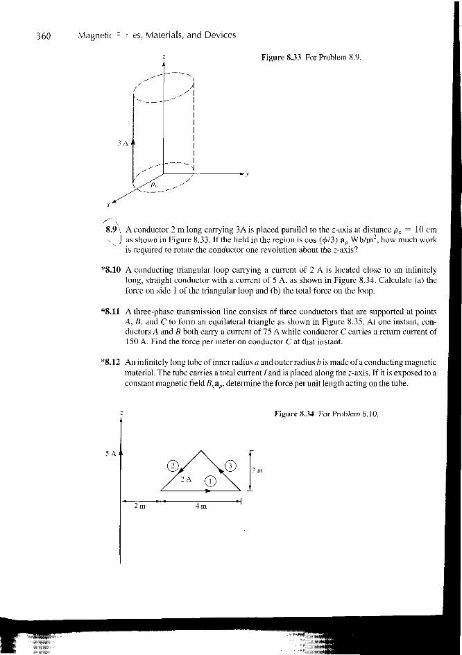
360 Magnetic -: -:es, Materials, and Devices
Figure 8.33 For Problem 8.9.
8.9 A conductor 2 m long carrying 3A is placed parallel to the z-axis at distance p0 = 10 cmas shown in Figure 8.33. If the field in the region is cos (4>/3) ap Wb/m2, how much workis required to rotate the conductor one revolution about the z-axis?
*8.10 A conducting triangular loop carrying a current of 2 A is located close to an infinitelylong, straight conductor with a current of 5 A, as shown in Figure 8.34. Calculate (a) theforce on side 1 of the triangular loop and (b) the total force on the loop.
*8.11 A three-phase transmission line consists of three conductors that are supported at pointsA, B, and C to form an equilateral triangle as shown in Figure 8.35. At one instant, con-ductors A and B both carry a current of 75 A while conductor C carries a return current of150 A. Find the force per meter on conductor C at that instant.
*8.12 An infinitely long tube of inner radius a and outer radius b is made of a conducting magneticmaterial. The tube carries a total current / and is placed along the z-axis. If it is exposed to aconstant magnetic field Boap, determine the force per unit length acting on the tube.
5 A
Figure 8.34 For Problem 8.10.
.©
2m 4 m

2m
B | 7 5 A
PROBLEMS
Figure 8.35 For Problem 8.11.
361
*8.13 An infinitely long conductor is buried but insulated from an iron mass (fi = 2000^,o) asshown in Figure 8.36. Using image theory, estimate the magnetic flux density at point P.
8.14 A galvanometer has a rectangular coil of side 10 by 30 mm pivoted about the center of theshorter side. It is mounted in radial magnetic field so that a constant magnetic field of 0.4Wb/m always acts across the plane of the coil. If the coil has 1000 turns and carriescurrent 2 mA, find the torque exerted on it.
= - 0 . 5 a , mWb/m2at(10, 0, 0). FindB8.15 A small magnet placed at the origin produces Bat
(a) (0 ,3 ,0)
(b) (3, 4, 0)
(c) ( 1 , 1 , - D
8.16 A block of iron (/* = 5000;uo) is placed in a uniform magnetic field with 1.5 Wb/m . Ifiron consists of 8.5 X 1028 atoms/m3, calculate: (a) the magnetization M, (b) the averagemagnetic current.
y
30 mm
o
p%-
0 A
20 mm
iron
20 mm \
*-x
Figure 8.36 For Problem 8.13.

362 Magnetic Forces, Materials, and Devices
8.17 In a certain material for which n = 6.5/x0,
H = 10ax + 25av - 40az A/m
find
(a) The magnetic susceptibility xm of the material
(b) The magnetic flux density B
(c) The magnetization M,
(d) The magnetic energy density
8.18 In a ferromagnetic material (/* = 4.5/to),
B = 4>-a_ mWb/m2
calculate: (a) Xm, (b) H, (c) M, (d) Jb.
8.19 The magnetic field intensity is H = 1200 A/m in a material when B = 2 Wb/m2. WhenH is reduced to 400 A/m, B = 1.4 Wb/m2. Calculate the change in the magnetization M.
8.20 An infinitely long cylindrical conductor of radius a and permeability /xo/xr is placed alongthe z-axis. If the conductor carries a uniformly distributed current / along a7 find M and Jb
for 0 < p < a.
8.21 If M = — {—y&x + xay) in a cube of size a, find Jb. Assume ko is a constant.
*8.22 (a) For the boundary between two magnetic media such as is shown in Figure 8.16, showthat the boundary conditions on the magnetization vector are
Mu M2t= K and • m l n =
Xml Xml Xm\ Xml
(b) If the boundary is not current free, show that instead of eq. (8.49), we obtain
tan 0, HI [
tan 62 L B-, sin d7
8.23 If Mi = 2fio for region 1 (0 < <j> < it) and p.2 = 5/*o for region 2 (IT < tj> < 2ir) andB2 = 10ap + 15a0 - 20az mWb/m2. Calculate: (a) B,, (b) the energy densities in thetwo media.
8.24 The interface 2x + y = 8 between two media carries no current. If medium1 (2x + y > 8) is nonmagnetic with H | = — 4aA + 3av — az A/m. Find: (a) the mag-netic energy density in medium 1, (b) M2 and B2 in medium 2 (2x + ^ £ 8 ) withH = 10/io, (c) the angles H] and H2 make with the normal to the interface.
8.25 The interface 4x — 5z = 0 between two magnetic media carries current 35av A/m. IfH] = 25ax — 30av + 45a, A/m in region 4x — 5z < 0 where firl = 5, calculate H2 inregion 4x — 5z — 0 where fir2 = 10.

TPROBLEMS 363
8.26 The plane z = 0 separates air (z > 0, y, = / O from iron (z < 0, ^ = 2 0 0 , 0 . Given that
H = 10ax + 15av - 3a, A/m
in air, find B in iron and the angle it makes with the interface.
8.27 Region 0 s ? < 2 m is filled with an infinite slab of magnetic material (fi = 2.5juo). Ifthe surfaces of the slab at z = 0 and z = 2, respectively, carry surface currents 30a,- A/mand — 40av A/m as in Figure 8.37, calculate H and B for
(a) z < 0
(b) 0 < z < 2
(c) z > 2
8.28 In a certain region for which x m = 19,
H = 5x2yzaA + 10xy2zav - 1 5 x y z V A/m
How much energy is stored in 0 < x < 1, 0 < v < 2, — 1 < z < 2 ?
18.29 The magnetization curve for an iron alloy is approximately given by B = —H +
H2n Wb/m2. Find: (a) \ir when H = 210 A/m, (b) the energy stored per unit volume inthe alloy as H increases from 0 to 210 A/m.
*8.30 (a) If the cross section of the toroid of Figure 7.15 is a square of side a, show that the self-inductance of the toroid is
L = In2po + a
(b) If the toroid has a circular cross section as in Figure 7.15, show that
L =
where p o ~^> a.
8.31 When two parallel identical wires are separated by 3 m, the inductance per unit length is2.5 juH/m. Calculate the diameter of each wire.
Mo
Figure 8.37 For Problem 8.27.
—40 ax A/m
z = 0 30 ax A/m

364 Magnetic Forces, Materials, and Devices
8.32 A solenoid with length 10 cm and radius 1 cm has 450 turns. Calculate its inductance.
8.33 The core of a toroid is 12 cm and is made of material with /xr = 200. If the mean radiusof the toroid is 50 cm, calculate the number of turns needed to obtain an inductance of2.5 H.
8.34 Show that the mutual inductance between the rectangular loop and the infinite line currentof Figure 8.4 is
r a + p0
Calculate M12 when a = b = po = 1 m.
*8.35 Prove that the mutual inductance between the closed wound coaxial solenoids of length <and €2 (^i ^ ^X turns Ny and N2, and radii r, and r2 with rx — r2 is
8.36 A cobalt ring (jxr = 600) has a mean radius of 30 cm. If a coil wound on the ring carries12 A, calculate the number of turns required to establish an average magnetic flux densityof 1.5 Wb/m in the ring.
8.37 Refer to Figure 8.27. If the current in the coil is 0.5 A, find the mmf and the magnetic fieldintensity in the air gap. Assume that [i = 500/no and that all branches have the samecross-sectional area of 10 cm2.
8.38 The magnetic circuit of Figure 8.38 has current 10 A in the coil of 2000 turns. Assume thatall branches have the same cross section of 2 cm2 and that the material of the core is ironwith nr = 1500. Calculate R, 9, and V for
(a) The core(b) The air gap
12 cm0.6 cm
Figure 8.38 For Problem 8.38.

0.2 A
("1
500 turns
-
»~
PROBLEMS
Figure 8.39 For Problem 8.39.
365
• L = 42 cm
8.39 Consider the magnetic circuit in Figure 8.39. Assuming that the core (^ = 1000/xo)hasauniform cross section of 4 cm2, determine the flux density in the air gap.
8.40 An electromagnetic relay is modeled as shown in Figure 8.40. What force is on the arma-ture (moving part) of the relay if the flux in the air gap is 2 mWb? The area of the gap is0.3 cm2, and its length 1.5 mm.
8.41 A toroid with air gap, shown in Figure 8.41, has a square cross section. A long conductorcarrying current 72 is inserted in the air gap. If 7, = 200 mA, N = 750, p0 = 10 cm,a = 5 mm, and ia = 1 mm, calculate
(a) The force across the gap when 72 = 0 and the relative permeability of the toroid is300
(b) The force on the conductor when 72 = 2 m A and the permeability of the toroid is in-finite. Neglect fringing in the gap in both cases.
8.42 A section of an electromagnet with a plate below it carrying a load is shown in Figure8.42. The electromagnet has a contact area of 200 cm2 per pole with the middle polehaving a winding of 1000 turns with 7 = 3 A. Calculate the maximum mass that can belifted. Assume that the reluctance of the electromagnet and the plate is negligible.
8.43 Figure 8.43 shows the cross section of an electromechanical system in which the plungermoves freely between two nonmagnetic sleeves. Assuming that all legs have the samecross-sectional area S, show that
F = 2 ^ 2 / 2 ^ a
(a + 2x^x
Figure 8.40 For Problem 8.40.

366 B Magnetic Forces, Materials, and Devices
Figure 8.41 For Problem 8.41.
Figure 8.42 For Problem 8.42.
1 mm
Figure 8.43 For Problem 8.43.
u J + •
-nmagnetic sleeve

PART 4
WAVES ANDAPPLICATIONS
Chapter y
MAXWELL'S EQUATIONS
Do you want to be a hero? Don't be the kind of person who watches others do
great things or doesn't know what's happening. Go out and make things happen.
The people who get things done have a burning desire to make things happen, get
ahead, serve more people, become the best they can possibly be, and help
improve the world around them.
—GLENN VAN EKEREN
9.1 INTRODUCTION
In Part II (Chapters 4 to 6) of this text, we mainly concentrated our efforts on electrostaticfields denoted by E(x, y, z); Part III (Chapters 7 and 8) was devoted to magnetostatic fieldsrepresented by H(JC, y, z). We have therefore restricted our discussions to static, or time-invariant, EM fields. Henceforth, we shall examine situations where electric and magneticfields are dynamic, or time varying. It should be mentioned first that in static EM fields,electric and magnetic fields are independent of each other whereas in dynamic EM fields,the two fields are interdependent. In other words, a time-varying electric field necessarilyinvolves a corresponding time-varying magnetic field. Second, time-varying EM fields,represented by E(x, y, z, t) and H(x, y, z, t), are of more practical value than static EMfields. However, familiarity with static fields provides a good background for understand-ing dynamic fields. Third, recall that electrostatic fields are usually produced by static elec-tric charges whereas magnetostatic fields are due to motion of electric charges withuniform velocity (direct current) or static magnetic charges (magnetic poles); time-varyingfields or waves are usually due to accelerated charges or time-varying currents such asshown in Figure 9.1. Any pulsating current will produce radiation (time-varying fields). Itis worth noting that pulsating current of the type shown in Figure 9.1(b) is the cause of ra-diated emission in digital logic boards. In summary:
charges —> electrostatic fieldssteady currenis —» magnclosiatic fieldstime-varying currenis ••» electromagnetic fields (or wavesj
Our aim in this chapter is to lay a firm foundation for our subsequent studies. This willinvolve introducing two major concepts: (1) electromotive force based on Faraday's ex-periments, and (2) displacement current, which resulted from Maxwell's hypothesis. As aresult of these concepts, Maxwell's equations as presented in Section 7.6 and the boundary
369

370 Maxwell's Equations
(a) (b)
(0
Figure 9.1 Various types of time-varying current: (a) sinusoidal,(b) rectangular, (c) triangular.
conditions for static EM fields will be modified to account for the time variation of thefields. It should be stressed that Maxwell's equations summarize the laws of electromag-netism and shall be the basis of our discussions in the remaining part of the text. For thisreason, Section 9.5 should be regarded as the heart of this text.
9.2 FARADAY'S LAW
After Oersted's experimental discovery (upon which Biot-Savart and Ampere based theirlaws) that a steady current produces a magnetic field, it seemed logical to find out if mag-netism would produce electricity. In 1831, about 11 years after Oersted's discovery,Michael Faraday in London and Joseph Henry in New York discovered that a time-varyingmagnetic field would produce an electric current.'
According to Faraday's experiments, a static magnetic field produces no current flow,but a time-varying field produces an induced voltage (called electromotive force or simplyemf) in a closed circuit, which causes a flow of current.
Faraday discovered that the induced emf. \\.iM (in volts), in any closed circuit isequal to the time rale of change of the magnetic flux linkage by the circuit.
This is called Faraday's law, and it can be expressed as
dt dt• e m f (9.1)
where N is the number of turns in the circuit and V is the flux through each turn. The neg-ative sign shows that the induced voltage acts in such a way as to oppose the flux produc-
'For details on the experiments of Michael Faraday (1791-1867) and Joseph Henry (1797-1878),see W. F. Magie, A Source Book in Physics. Cambridge, MA: Harvard Univ. Press, 1963, pp.472-519.

9.2 FARADAY'S LAW 371
battery
Figure 9.2 A circuit showing emf-producing fieldand electrostatic field E,.
ing it. This is known as Lenz's law,2 and it emphasizes the fact that the direction of currentflow in the circuit is such that the induced magnetic field produced by the induced currentwill oppose the original magnetic field.
Recall that we described an electric field as one in which electric charges experienceforce. The electric fields considered so far are caused by electric charges; in such fields, theflux lines begin and end on the charges. However, there are other kinds of electric fields notdirectly caused by electric charges. These are emf-produced fields. Sources of emf includeelectric generators, batteries, thermocouples, fuel cells, and photovoltaic cells, which allconvert nonelectrical energy into electrical energy.
Consider the electric circuit of Figure 9.2, where the battery is a source of emf. Theelectrochemical action of the battery results in an emf-produced field Ey. Due to the accu-mulation of charge at the battery terminals, an electrostatic field Ee{ = — VV) also exists.The total electric field at any point is
E = Ey + Ee (9.2)
Note that Ey is zero outside the battery, Ey and Ee have opposite directions in the battery,and the direction of Ee inside the battery is opposite to that outside it. If we integrateeq. (9.2) over the closed circuit,
E • d\ = <f Ey • d\ + 0 = Ef-dl (through battery) (9.3a)
where § Ee • d\ = 0 because Ee is conservative. The emf of the battery is the line integralof the emf-produced field; that is,
d\ = - (9.3b)
since Eyand Ee are equal but opposite within the battery (see Figure 9.2). It may also be re-garded as the potential difference (VP - VN) between the battery's open-circuit terminals.It is important to note that:
1. An electrostatic field Ee cannot maintain a steady current in a closed circuit since$LEe-dl = 0 = //?.
2. An emf-produced field Eyis nonconservative.3. Except in electrostatics, voltage and potential difference are usually not equivalent.
2After Heinrich Friedrich Emil Lenz (1804-1865), a Russian professor of physics.

372 B Maxwell's Equations
9.3 TRANSFORMER AND MOTIONAL EMFs
Having considered the connection between emf and electric field, we may examine howFaraday's law links electric and magnetic fields. For a circuit with a single turn (N = 1),eq. (9.1) becomes
V - ** (9.4)
In terms of E and B, eq. (9.4) can be written as
yemf = f E • d\ = - - Bh dt 4
(9.5)
where *P has been replaced by Js B • dS and S is the surface area of the circuit bounded bythe closed path L. It is clear from eq. (9.5) that in a time-varying situation, both electric andmagnetic fields are present and are interrelated. Note that d\ and JS in eq. (9.5) are in ac-cordance with the right-hand rule as well as Stokes's theorem. This should be observed inFigure 9.3. The variation of flux with time as in eq. (9.1) or eq. (9.5) may be caused in threeways:
1. By having a stationary loop in a time-varying B field2. By having a time-varying loop area in a static B field3. By having a time-varying loop area in a time-varying B field.
Each of these will be considered separately.
A. Stationary Loop in Time-Varying B Fit transformer emf)
This is the case portrayed in Figure 9.3 where a stationary conducting loop is in a time-varying magnetic B field. Equation (9.5) becomes
(9.6)
Increasing B(t) Figure 9.3 Induced emf due to a stationary loop in a time-varying B field.
:ed B

9.3 TRANSFORMER AND MOTIONAL EMFS 373
This emf induced by the time-varying current (producing the time-varying B field) in a sta-tionary loop is often referred to as transformer emf in power analysis since it is due totransformer action. By applying Stokes's theorem to the middle term in eq. (9.6), we obtain
(V X E) • dS = - I — • dS
For the two integrals to be equal, their integrands must be equal; that is,
(9.7)
dt(9.8)
This is one of the Maxwell's equations for time-varying fields. It shows that the time-varying E field is not conservative (V X E + 0). This does not imply that the principles ofenergy conservation are violated. The work done in taking a charge about a closed path ina time-varying electric field, for example, is due to the energy from the time-varying mag-netic field. Observe that Figure 9.3 obeys Lenz's law; the induced current / flows such asto produce a magnetic field that opposes B(f).
B. Moving Loop in Static B Field (Motional emf)
When a conducting loop is moving in a static B field, an emf is induced in the loop. Werecall from eq. (8.2) that the force on a charge moving with uniform velocity u in a mag-netic field B is
Fm = Qu X B
We define the motional electric field Em as
(8.2)
Em = - ^ = u X B (9.9)
If we consider a conducting loop, moving with uniform velocity u as consisting of a largenumber of free electrons, the emf induced in the loop is
(9.10)
This type of emf is called motional emf or flux-cutting emf because it is due to motionalaction. It is the kind of emf found in electrical machines such as motors, generators, and al-ternators. Figure 9.4 illustrates a two-pole dc machine with one armature coil and a two-bar commutator. Although the analysis of the d.c. machine is beyond the scope of this text,we can see that voltage is generated as the coil rotates within the magnetic field. Anotherexample of motional emf is illustrated in Figure 9.5, where a rod is moving between a pair

374 11 Maxwell's Equations
Figure 9.4 A direct-current machine.
of rails. In this example, B and u are perpendicular, so eq. (9.9) in conjunction witheq. (8.2) becomes
or
and eq. (9.10) becomes
Fm = U X B
Fm = KB
Vem( =
By applying Stokes's theorem to eq. (9.10)
( V X E J ' d S = V X (u X B) • dS's 's
or
V X Em = V X (u X B)
(9.11)
(9.12)
(9.13)
(9.14)
Notice that unlike eq. (9.6), there is no need for a negative sign in eq. (9.10) becauseLenz's law is already accounted for.
B(in)Figure 9.5 Induced emf due to a movingloop in a static B field.

9.3 TRANSFORMER AND MOTIONAL EMFS 375
To apply eq. (9.10) is not always easy; some care must be exercised. The followingpoints should be noted:
1. The integral in eq. (9.10) is zero along the portion of the loop where u = 0. Thusd\ is taken along the portion of the loop that is cutting the field (along the rod inFigure 9.5), where u has nonzero value.
2. The direction of the induced current is the same as that of Em or u X B. The limitsof the integral in eq. (9.10) are selected in the opposite direction to the inducedcurrent thereby satisfying Lenz's law. In eq. (9.13), for example, the integrationover L is along —av whereas induced current flows in the rod along ay.
C. Moving Loop in Time-Varying Field
This is the general case in which a moving conducting loop is in a time-varying magneticfield. Both transformer emf and motional emf are present. Combining eqs. (9.6) and (9.10)gives the total emf as
(9.15)f
V f = 9J E •d\ =f flB ft (u X B) •d\
or from eqs. (9.8) and (9.14),
V X E = + V X (u X B)dt
(9.16)
Note that eq. (9.15) is equivalent to eq. (9.4), so Vemf can be found using either eq. (9.15)or (9.4). In fact, eq. (9.4) can always be applied in place of eqs. (9.6), (9.10), and (9.15).
EXAMPLE 9.1A conducting bar can slide freely over two conducting rails as shown in Figure 9.6. Calcu-late the induced voltage in the bar
(a) If the bar is stationed at y = 8 cm and B = 4 cos 106f az mWb/m2
(b) If the bar slides at a velocity u = 20aj, m/s and B = 4az mWb/m2
(c) If the bar slides at a velocity u = 20ay m/s and B = 4 cos (106r — y) az mWb/m2
Figure 9.6 For Example 9.1.
0
6 cm
©
©B
©
©
0 ©
0 ©

376 Maxwell's Equations
Solution:
(a) In this case, we have transformer emf given by
dB
dtdS =
0.08 /-0.06
y=0
sin Wtdxdy
= 4(103)(0.08)(0.06) sin l06t= 19.2 sin 106;V
The polarity of the induced voltage (according to Lenz's law) is such that point P on thebar is at lower potential than Q when B is increasing.
(b) This is the case of motional emf:
Vemf = (" x B) • d\ = {u&y X Baz) • dxax
= -uB( = -20(4.10"3)(0.06)= -4.8 mV
(c) Both transformer emf and motional emf are present in this case. This problem can besolved in two ways.
Method 1: Using eq. (9.15)
Kmf = " I — • dS + | (U X B) • d\
r0.06 ry
(9.1.1)
x=0 ""00
[20ay X 4.10 3 cos(106f - y)aj • dxax
0.06
= 240 cos(106f - / ) - 80(10~3)(0.06) cos(106r - y)
= 240 008(10"? - y) - 240 cos 106f - 4.8(10~j) cos(106f - y)=- 240 cos(106f -y)- 240 cos 106? (9.1.2)
because the motional emf is negligible compared with the transformer emf. Using trigono-metric identity
A + B A - Bcos A - cos B = - 2 sin sin — - —
Veirf = 480 sin MO6? - £ ) sin ^ V (9.1.3)

9.3 TRANSFORMER AND MOTIONAL EMFS
Method 2: Alternatively we can apply eq. (9.4), namely,
Vemt = ~
where
dt
377
(9.1.4)
B-dS
•0.06
4 cos(106r - y) dx dyy=0 JJt=
= -4(0.06) sin(106f - y)
= -0.24 sin(106r - y) + 0.24 sin 10°f mWb
But
Hence,
— = u -> y = ut = 20/
V = -0.24 sin(106r - 200 + 0.24 sin 106f mWb
yemf = = 0.24(106 - 20) cos(106r - 20f) - 0.24(106) cos 106f mVdt
= 240 cos(106f - y) - 240 cos 106f V (9.1.5)
which is the same result in (9.1.2). Notice that in eq. (9.1.1), the dependence of y on timeis taken care of in / (u X B) • d\, and we should not be bothered by it in dB/dt. Why?Because the loop is assumed stationary when computing the transformer emf. This is asubtle point one must keep in mind in applying eq. (9.1.1). For the same reason, the secondmethod is always easier.
PRACTICE EXERCISE 9.1
Consider the loop of Figure 9.5. If B = 0.5az Wb/m2, R = 20 0, € = 10 cm, and therod is moving with a constant velocity of 8ax m/s, find
(a) The induced emf in the rod
(b) The current through the resistor
(c) The motional force on the rod
(d) The power dissipated by the resistor.
Answer: (a) 0.4 V, (b) 20 mA, (c) - a x mN, (d) 8 mW.

378 • Maxwell's Equations
EXAMPLE 9.2The loop shown in Figure 9.7 is inside a uniform magnetic field B = 50 ax mWb/m2. Ifside DC of the loop cuts the flux lines at the frequency of 50 Hz and the loop lies in thejz-plane at time t = 0, find
(a) The induced emf at t = 1 ms
(b) The induced current at t = 3 ms
Solution:
(a) Since the B field is time invariant, the induced emf is motional, that is,
yemf = (u x B) • d\
where
d\ = d\DC = dzaz, u =dt dt
p = AD = 4 cm, a) = 2TT/ = IOOTT
As u and d\ are in cylindrical coordinates, we transform B into cylindrical coordinatesusing eq. (2.9):
B = BQax = Bo (cos <j> ap - sin <t> a0)
where Bo = 0.05. Hence,
u X B = 0 pco 0Bo cos 4> —Bo sin 4> 0
= —puBo cos </> az
Figure 9.7 For Example 9.2; polarity is forincreasing emf.

9.3 TRANSFORMER AND MOTIONAL EMFS • 379
and
(uXB)-dl= -puBo cos <f> dz = - 0 . 0 4 ( 1 0 0 T T ) ( 0 . 0 5 ) COS <t> dz= —0.2-ir cos 0 dz
r 0.03
V e m f = — 0 .2TT COS 4> dz = — 6TT COS <f> m V4=0
To determine <j>, recall that
d<t>co = > 0 = cof + C odt
where Co is an integration constant. At t = 0, 0 = TT/2 because the loop is in the yz-planeat that time, Co = TT/2. Hence,
= CO/ +TT
and
mf = ~6TT cosf cor + — ) = 6TT sin(lOOirf) mV
At f = 1 ms, yemf = 6TT sin(O.lTr) = 5.825 mV
(b) The current induced is
. Vem{
R= 607rsin(100xr)mA
At t = 3 ms,
i = 60TT sin(0.37r) mA = 0.1525 A
PRACTICE EXERCISE 9.2
Rework Example 9.2 with everything the same except that the B field is changed to:
(a) B = 50av. mWb/m2—that is, the magnetic field is oriented along the y-direction
(b) B = 0.02ir ax Wb/m2—that is, the magnetic field is time varying.
Answer: (a) -17.93 mV, -0.1108 A, (b) 20.5 jtV, -41.92 mA.
EXAMPLE 9.3The magnetic circuit of Figure 9.8 has a uniform cross section of 10 3 m2. If the circuit isenergized by a current ix{i) = 3 sin IOOTT? A in the coil of N\ = 200 turns, find the emfinduced in the coil of N2 = 100 turns. Assume that JX. = 500 /xo.

380 11 Maxwell's Equations
/Ah(o / r
" l lpo = 10 cm <LJN2
<Dl\
Solution:
The flux in the circuit is
w — —
Figure 9.8 Magnetic circuit ofExample 9.3.
-o +
2irpo
According to Faraday's law, the emf induced in the second coil is
V2 = -N2 —r = — ~ -dt 2-Kp0 dt
100 • (200) • (500) • (4TT X 10"7) • (10~3) • 300TT COS IOOTT?
2x • (10 X 10"2)= -6TTCOS 100ir?V
PRACTICE EXERCISE 9.3
A magnetic core of uniform cross section 4 cm2 is connected to a 120-V, 60-Hzgenerator as shown in Figure 9.9. Calculate the induced emf V2 in the second-ary coil.
Aaswer: 72 V
Vtfc)
Ti
> N2 = 300 V2
Figure 9.9 For Practice Exercise 9.3.

9.4 DISPLACEMENT CURRENT 381
9.4 DISPLACEMENT CURRENT
In the previous section, we have essentially reconsidered Maxwell's curl equation for elec-trostatic fields and modified it for time-varying situations to satisfy Faraday's law. We shallnow reconsider Maxwell's curl equation for magnetic fields (Ampere's circuit law) fortime-varying conditions.
For static EM fields, we recall that
V x H = J (9.17)
But the divergence of the curl of any vector field is identically zero (see Example 3.10).Hence,
V - ( V X H ) = 0 = V - J
The continuity of current in eq. (5.43), however, requires that
(9.18)
(9.19)
Thus eqs. (9.18) and (9.19) are obviously incompatible for time-varying conditions. Wemust modify eq. (9.17) to agree with eq. (9.19). To do this, we add a term to eq. (9.17) sothat it becomes
V X H = J + Jd (9.20)
where id is to be determined and defined. Again, the divergence of the curl of any vector iszero. Hence:
In order for eq. (9.21) to agree with eq. (9.19),
(9.21)
(9.22a)
or
h
3.20) results
V X H =
dD
dt
in
.1 +dX)
dt
(9.22b)
(9.23)
This is Maxwell's equation (based on Ampere's circuit law) for a time-varying field. Theterm Jd = dD/dt is known as displacement current density and J is the conduction current
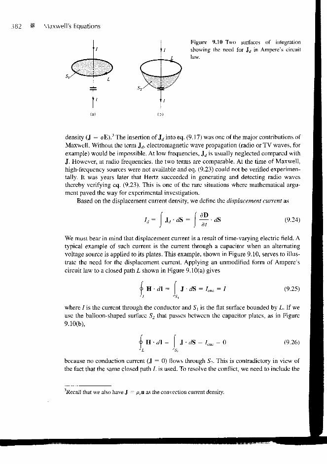
382 • Maxwell's Equations
(a)
Figure 9.10 Two surfaces of integration/ showing the need for Jd in Ampere's circuit
law.
density (J = aE).3 The insertion of Jd into eq. (9.17) was one of the major contributions ofMaxwell. Without the term Jd, electromagnetic wave propagation (radio or TV waves, forexample) would be impossible. At low frequencies, Jd is usually neglected compared withJ. However, at radio frequencies, the two terms are comparable. At the time of Maxwell,high-frequency sources were not available and eq. (9.23) could not be verified experimen-tally. It was years later that Hertz succeeded in generating and detecting radio wavesthereby verifying eq. (9.23). This is one of the rare situations where mathematical argu-ment paved the way for experimental investigation.
Based on the displacement current density, we define the displacement current as
ld= \jd-dS =dt
dS (9.24)
We must bear in mind that displacement current is a result of time-varying electric field. Atypical example of such current is the current through a capacitor when an alternatingvoltage source is applied to its plates. This example, shown in Figure 9.10, serves to illus-trate the need for the displacement current. Applying an unmodified form of Ampere'scircuit law to a closed path L shown in Figure 9.10(a) gives
(9.25)H d\ = J • dS = /enc = /
where / is the current through the conductor and Sx is the flat surface bounded by L. If weuse the balloon-shaped surface S2 that passes between the capacitor plates, as in Figure9.10(b),
(9.26)H d\ = J • dS = Ieac = 0
4because no conduction current (J = 0) flows through S2- This is contradictory in view ofthe fact that the same closed path L is used. To resolve the conflict, we need to include the
• Recall that we also have J = pvii as the convection current density.

9.4 DISPLACEMENT CURRENT 383
displacement current in Ampere's circuit law. The total current density is J + Jd. Ineq. (9.25), id = 0 so that the equation remains valid. In eq. (9.26), J = 0 so that
H d\ = I id • dS = =- I D • dS = -~ = Idt dt
(9.27)
So we obtain the same current for either surface though it is conduction current in S{ anddisplacement current in S2.
EXAMPLE 9.4A parallel-plate capacitor with plate area of 5 cm2 and plate separation of 3 mm has avoltage 50 sin 103r V applied to its plates. Calculate the displacement current assuminge = 2eo.
Solution:
D = eE = s —d
dDdt
e dv~d dt
Hence,
which is the same as the conduction current, given by
/ = 2
s
dt dt
5
dt
36TT 3 X 10"3
=
dt d dt
103 X 50 cos 10't
dV
dt
= 147.4 cos 103?nA
PRACTICE EXERCISE 9.4
In free space, E = 20 cos (at - 50xj ay V/m. Calculate
(a) h
(b) H
(c) w
Answer: (a) -20a>so sin (wt - 50J:) ay A/m2, (b) 0.4 wso cos(uit - 50x) az A/m,(c)1.5 X 1010rad/s.
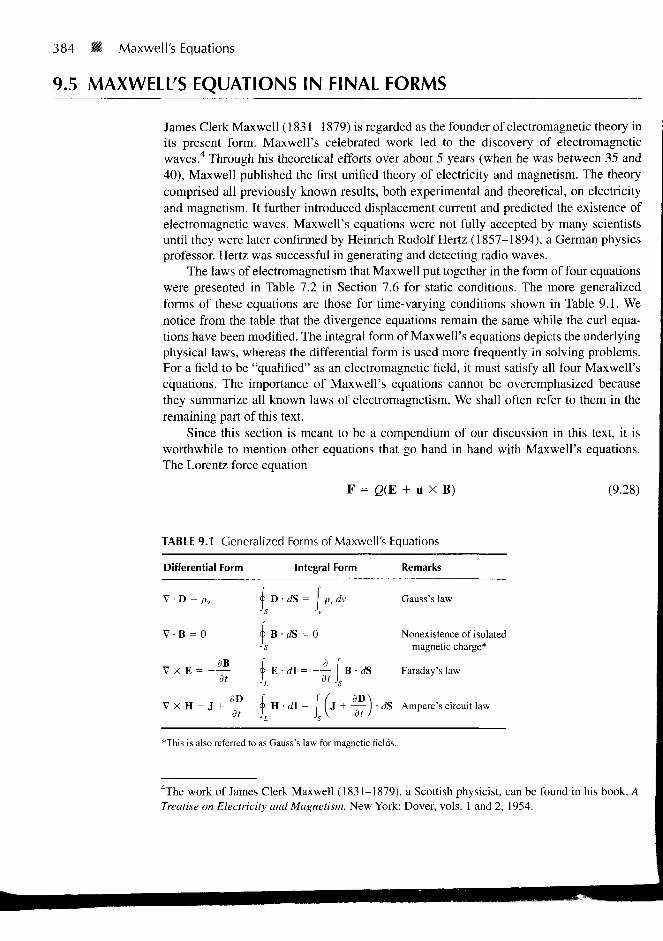
384 • Maxwell's Equations
9.5 MAXWELL'S EQUATIONS IN FINAL FORMS
James Clerk Maxwell (1831-1879) is regarded as the founder of electromagnetic theory inits present form. Maxwell's celebrated work led to the discovery of electromagneticwaves.4 Through his theoretical efforts over about 5 years (when he was between 35 and40), Maxwell published the first unified theory of electricity and magnetism. The theorycomprised all previously known results, both experimental and theoretical, on electricityand magnetism. It further introduced displacement current and predicted the existence ofelectromagnetic waves. Maxwell's equations were not fully accepted by many scientistsuntil they were later confirmed by Heinrich Rudolf Hertz (1857-1894), a German physicsprofessor. Hertz was successful in generating and detecting radio waves.
The laws of electromagnetism that Maxwell put together in the form of four equationswere presented in Table 7.2 in Section 7.6 for static conditions. The more generalizedforms of these equations are those for time-varying conditions shown in Table 9.1. Wenotice from the table that the divergence equations remain the same while the curl equa-tions have been modified. The integral form of Maxwell's equations depicts the underlyingphysical laws, whereas the differential form is used more frequently in solving problems.For a field to be "qualified" as an electromagnetic field, it must satisfy all four Maxwell'sequations. The importance of Maxwell's equations cannot be overemphasized becausethey summarize all known laws of electromagnetism. We shall often refer to them in theremaining part of this text.
Since this section is meant to be a compendium of our discussion in this text, it isworthwhile to mention other equations that go hand in hand with Maxwell's equations.The Lorentz force equation
+ u X B) (9.28)
TABLE 9.1 Generalized Forms of Maxwell's Equations
Differential
V • D = pv
V - B = O
V X E = -
V X H = J
Form
3B
dt
3D
at
1 D's
9 B
I,*<P H'L
Integral
• dS = j p,
rfS = 0
dt
Form
,rfv
B-rfS
Remarks
Gauss's law
Nonexistence of isolatedmagnetic charge*
Faraday's law
• dS Ampere's circuit law
*This is also referred to as Gauss's law for magnetic fields.
4The work of James Clerk Maxwell (1831-1879), a Scottish physicist, can be found in his book, ATreatise on Electricity and Magnetism. New York: Dover, vols. 1 and 2, 1954.
9.5 MAXWELL'S EQUATIONS IN FINAL FORMS M 385
is associated with Maxwell's equations. Also the equation of continuity
V • J = - — (9.29)dt
is implicit in Maxwell's equations. The concepts of linearity, isotropy, and homogeneity ofa material medium still apply for time-varying fields; in a linear, homogeneous, andisotropic medium characterized by a, e, and fi, the constitutive relations
D = eE = eoE + P
B = ixH = /no(H + M)
J = CTE + pvu
hold for time-varying fields. Consequently, the boundary conditions
Eu = E2t or (Ej - E2) X anl2 = 0
# u ~ H2t = K or (H, - H2) X anl2 = K
Din - D2n = p, or (D, - D2) • an l2 = p,
Bm - B2n = 0 or (B2 - B,) • aBl2 = 0
(9.30a)
(9.30b)
(9.30c)
(9.31a)
(9.31b)
(9.31c)
(9.31d)
remain valid for time-varying fields. However, for a perfect conductor (a — °°) in a time-varying field,
and hence,
E = 0, H = 0, J = 0
BB = 0, E, = 0
(9.32)
(9.33)
For a perfect dielectric (a — 0), eq. (9.31) holds except that K = 0. Though eqs. (9.28) to(9.33) are not Maxwell's equations, they are associated with them.
To complete this summary section, we present a structure linking the various poten-tials and vector fields of the electric and magnetic fields in Figure 9.11. This electromag-netic flow diagram helps with the visualization of the basic relationships between fieldquantities. It also shows that it is usually possible to find alternative formulations, for agiven problem, in a relatively simple manner. It should be noted that in Figures 9.10(b) and(c), we introduce pm as the free magnetic density (similar to pv), which is, of course, zero,Ae as the magnetic current density (analogous to J). Using terms from stress analysis, theprincipal relationships are typified as:
(a) compatibility equations
V • B = pm = 0 (9.34)

386 • Maxwell's Eolations
^ -v«v
(a)
Vx—Vx 0Vx ' Vx
V-'
(b) (c)
Figure 9.11 Electromagnetic flow diagram showing the relationship between the potentialsand vector fields: (a) electrostatic system, (b) magnetostatic system, (c) electromagneticsystem. [Adapted with permission from IEE Publishing Dept.]
and
(b) constitutive equations
and
(c) equilibrium equations
and
B = ,uH
D = eE
V • D = Pv
dt

9.6 TIME-VARYING POTENTIALS 387
9.6 TIME-VARYING POTENTIALS
For static EM fields, we obtained the electric scalar potential as
pvdv
and the magnetic vector potential as
V =
A =
AireR
fiJ dv
4wR
(9.40)
(9.41)
We would like to examine what happens to these potentials when the fields are timevarying. Recall that A was defined from the fact that V • B = 0, which still holds for time-varying fields. Hence the relation
B = V X A (9.42)
holds for time-varying situations. Combining Faraday's law in eq. (9.8) with eq. (9.42) gives
V X E = (V X A) (9.43a)
or
V X | E + - | =dt
(9.43b)
Since the curl of the gradient of a scalar field is identically zero (see Practice Exercise3.10), the solution to eq. (9.43b) is
dt
or
dt
(9.44)
(9.45)
From eqs. (9.42) and (9.45), we can determine the vector fields B and E provided that thepotentials A and V are known. However, we still need to find some expressions for A andV similar to those in eqs. (9.40) and (9.41) that are suitable for time-varying fields.
From Table 9.1 or eq. (9.38) we know that V • D = pv is valid for time-varying condi-tions. By taking the divergence of eq. (9.45) and making use of eqs. (9.37) and (9.38), weobtain
V - E = — = - V 2 V - — ( V - A )e dt
388 Maxwell's Equations
or
VV + ( V A )dt e
Taking the curl of eq. (9.42) and incorporating eqs. (9.23) and (9.45) results in
VX V X A = uj + e/n — ( -VVdt V dt
dV
(9.46)
where D = sE and B = fiH have been assumed. By applying the vector identity
V X V X A = V(V • A) - V2A
to eq. (9.47),
V2A - V(V • A) = -f + \dt
d2A—r-dt2
(9.47)
(9.48)
(9.49)
A vector field is uniquely defined when its curl and divergence are specified. The curl of Ahas been specified by eq. (9.42); for reasons that will be obvious shortly, we may choosethe divergence of A as
V • A = -JdV_
dt(9.50)
This choice relates A and V and it is called the Lorentz condition for potentials. We had thisin mind when we chose V • A = 0 for magnetostatic fields in eq. (7.59). By imposing theLorentz condition of eq. (9.50), eqs. (9.46) and (9.49), respectively, become
(9.51)
and
2
V2A JUS
d2V
dt2
a2 A
dt2
Pve
y
/xj (9.52)
which are wave equations to be discussed in the next chapter. The reason for choosing theLorentz condition becomes obvious as we examine eqs. (9.51) and (9.52). It uncoupleseqs. (9.46) and (9.49) and also produces a symmetry between eqs. (9.51) and (9.52). It canbe shown that the Lorentz condition can be obtained from the continuity equation; there-fore, our choice of eq. (9.50) is not arbitrary. Notice that eqs. (6.4) and (7.60) are specialstatic cases of eqs. (9.51) and (9.52), respectively. In other words, potentials V and Asatisfy Poisson's equations for time-varying conditions. Just as eqs. (9.40) and (9.41) are

9.7 TIME-HARMONIC FIELDS 389
the solutions, or the integral forms of eqs. (6.4) and (7.60), it can be shown that the solu-tions5 to eqs. (9.51) and (9.52) are
V =[P.] dv
A-KSR
and
A =A-KR
(9.53)
(9.54)
The term [pv] (or [J]) means that the time t in pv(x, y, z, t) [or J(x, y, z, t)] is replaced by theretarded time t' given by
(9.55)
where R = |r — r ' | is the distance between the source point r ' and the observation point rand
1u = (9.56)
/xe
is the velocity of wave propagation. In free space, u = c — 3 X 1 0 m/s is the speed oflight in a vacuum. Potentials V and A in eqs. (9.53) and (9.54) are, respectively, called theretarded electric scalar potential and the retarded magnetic vector potential. Given pv andJ, V and A can be determined using eqs. (9.53) and (9.54); from V and A, E and B can bedetermined using eqs. (9.45) and (9.42), respectively.
9.7 TIME-HARMONIC FIELDS
So far, our time dependence of EM fields has been arbitrary. To be specific, we shallassume that the fields are time harmonic.
A time-harmonic field is one thai varies periodically or sinusoidally wiih time.
Not only is sinusoidal analysis of practical value, it can be extended to most waveforms byFourier transform techniques. Sinusoids are easily expressed in phasors, which are moreconvenient to work with. Before applying phasors to EM fields, it is worthwhile to have abrief review of the concept of phasor.
Aphasor z is a complex number that can be written as
z = x + jy = r (9.57)
1983, pp. 291-292.
390 Maxwell's Equations
or„ = r „)<$> == r e = r (cos <j> + j sin - (9.58)
where j = V — 1, x is the real part of z, y is the imaginary part of z, r is the magnitude ofz, given by
r —
and cj> is the phase of z, given by
= tan'1 l
(9.59)
(9.60)
Here x, y, z, r, and 0 should not be mistaken as the coordinate variables although theylook similar (different letters could have been used but it is hard to find better ones). Thephasor z can be represented in rectangular form as z = x + jy or in polar form asz = r [§_ = r e'^. The two forms of representing z are related in eqs. (9.57) to (9.60) andillustrated in Figure 9.12. Addition and subtraction of phasors are better performed in rec-tangular form; multiplication and division are better done in polar form.
Given complex numbers
z = x + jy = r[$_, z, = x, + jy, = r, /
the following basic properties should be noted.
Addition:
Subtraction:
Multiplication:
Division:
x2)
x2)
and z2 = x2 + jy2 = r2 /<j>2
y2) (9.61a)
- y2) (9.61b)
(9.61c)
(9.61d)
lm
co rad/s
Figure 9.12 Representation of a phasor z = x + jyr /<t>.
•Re

9.7 TIME-HARMONIC FIELDS H 391
Square Root:
Complex Conjugate:
Z = Vr
Z* = x — jy = r/—<j> == re
Other properties of complex numbers can be found in Appendix A.2.To introduce the time element, we let
(9.61e)
(9.61f)
(9.62)
where 6 may be a function of time or space coordinates or a constant. The real (Re) andimaginary (Im) parts of
= rejeeJo"
are, respectively, given by
and
Re (rej<t>) = r cos (ut + 0)
Im {rei4>) = r sin (art + 0)
(9.63)
(9.64a)
(9.64b)
Thus a sinusoidal current 7(0 = 7O cos(wt + 0), for example, equals the real part ofIoe
jeeM. The current 7'(0 = h sin(co? + 0), which is the imaginary part of Ioe]ee]01t, can
also be represented as the real part of Ioejeeju"e~j90° because sin a = cos(a - 90°).
However, in performing our mathematical operations, we must be consistent in our use ofeither the real part or the imaginary part of a quantity but not both at the same time.
The complex term Ioeje, which results from dropping the time factor ejo" in 7(0, is
called the phasor current, denoted by 7 ; that is,
]s = io(,J» = 70 / 0 (9.65)
where the subscript s denotes the phasor form of 7(0- Thus 7(0 = 70 cos(cof + 0), the in-stantaneous form, can be expressed as
= Re (9.66)
In general, a phasor could be scalar or vector. If a vector A(*, y, z, t) is a time-harmonicfield, the phasor form of A is As(x, y, z); the two quantities are related as
A = Re (XseJo")
For example, if A = Ao cos (ut — j3x) ay, we can write A as
A = Re (Aoe-j0x a / u ' )
Comparing this with eq. (9.67) indicates that the phasor form of A is
(9.67)
(9.68)
**-s AQ€ (9.69)

392 M Maxwell's Equations
Notice from eq. (9.67) that
(9.70)= Re (/«A/M()
showing that taking the time derivative of the instantaneous quantity is equivalent to mul-tiplying its phasor form byyco. That is,
<3A
Similarly,
(9.71)
(9.72)
Note that the real part is chosen in eq. (9.67) as in circuit analysis; the imaginary partcould equally have been chosen. Also notice the basic difference between the instanta-neous form A(JC, y, z, t) and its phasor form As(x, y, z); the former is time dependent andreal whereas the latter is time invariant and generally complex. It is easier to work with Aand obtain A from As whenever necessary using eq. (9.67).
We shall now apply the phasor concept to time-varying EM fields. The fields quanti-ties E(x, y, z, t), D(x, y, z, t), H(x, y, z, t), B(x, y, z, t), J(x, y, z, t), and pv(x, y, z, i) and theirderivatives can be expressed in phasor form using eqs. (9.67) and (9.71). In phasor form,Maxwell's equations for time-harmonic EM fields in a linear, isotropic, and homogeneousmedium are presented in Table 9.2. From Table 9.2, note that the time factor eJa" disappearsbecause it is associated with every term and therefore factors out, resulting in time-independent equations. Herein lies the justification for using phasors; the time factor canbe suppressed in our analysis of time-harmonic fields and inserted when necessary. Alsonote that in Table 9.2, the time factor e'01' has been assumed. It is equally possible to haveassumed the time factor e~ja", in which case we would need to replace every y in Table 9.2with —j.
TABLE 9.2 Time-Harmonic Maxwell's EquationsAssuming Time Factor e'""
Point Form Integral Form
Dv • dS = I pvs dv
B5 • dS = 0
V • D v = />„.,
V • B.v = 0
V X E s = -joiB, <k E s • d\ = -ju> I Bs • dS
V X H, = Js + juDs §Hs-dl= [ (J s + joiDs) • dS

9.7 TIME-HARMONIC FIELDS 393
EXAMPLE 9.5Evaluate the complex numbers
7(3 - ;4)*(a) z, =
( -111/2
Solution:
(a) This can be solved in two ways: working with z in rectangular form or polar form.
Method 1: (working in rectangular form):Let
_ Z3Z4
where
£3 =j
z,4 = (3 - j4)* = the complex conjugate of (3 - j4)= 3 + ;4
(To find the complex conjugate of a complex number, simply replace every) with —j.)
z5 = - 1 +76
and
Hence,
z3z4 = j4) = - 4
and
= (-1 + j6)(3 + ;4) = - 3 - ;4= -27+ ;14
- 4 + ;3
- 24
*"' - 2 7 + 7 I 4
Multiplying and dividing z\ by -27 - j\4 (rationalization), we have
(-4 + j3)(-27 - yi4) _ 150 -J25Zl ~ (-27 +yl4)(-27 -j'14) 272 + 142
= 0.1622 -;0.027 = 0.1644 / - 9.46°
Method 2: (working in polar form):
z3=j= 1/90°
z4 = (3 - j4)* = 5 /-53.130)* = 5 /53.13°
394 • Maxwell's Equations
Hence,
as obtained before,
(b) Let
where
and
Hence
z5 = ("I +j6) = V37 /99.46°
zb = (2 + jf = (V5 /26.56°)2 = 5 /53.130
(1 /90°)(5 /53.130)
and
(V37 /99.46°)(5 /53.130)
1 /90° - 99.46° = 0.1644 /-9.46°V37
= 0.1622 - 70.027
1/2
Zs
Z7=l+j= V2/45°
= 4 -78 = 4V5/-63.4O
V2 /45° V2
4V5/-63.40 4V50.1581 7108.4°
/45° 63.4°
z2 = V0.1581 /108.472= 0.3976 754.2°
PRACTICE EXERCISE 9.5
Evaluate these complex numbers:
(b) 6 /W_ + ;5 - 3 + ejn
Answer: (a) 0.24 + j0.32, (b) 2.903 + J8.707.
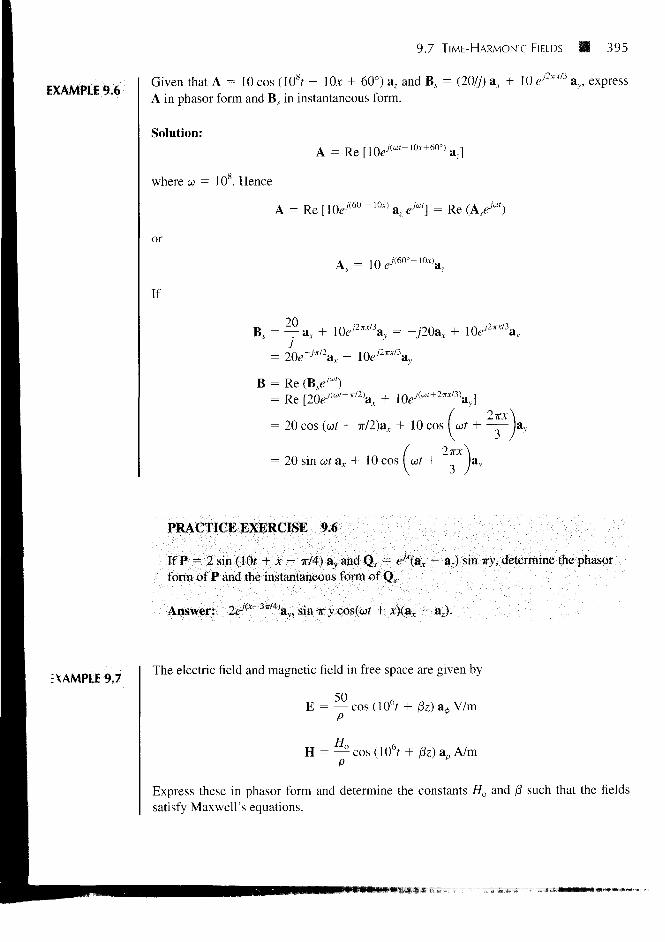
9.7 TIME-HARMONIC FIELDS • 395
EXAMPLE 9.6Given that A = 10 cos (108? - 10* + 60°) az and Bs = (20//) a, + 10 ej2"B ay, expressA in phasor form and B^ in instantaneous form.
Solution:
where u = 10 . Hence
A = Re[10e'M~1 0 A H
If
A = Re [\0eJ(bU ~lw az e*"] = Re ( A , O
A, = ]0ej
90e / 2" / 3a = - jB, = — a , + 10e / 2" / 3ay = - j20a v
2 / 2 / 3
B = Re (B.e-"0')= Re [20ej(w("7r/2)ax + lO^'(w'+2TJ[/3)a),]
/ 2TT*\= 20 cos (art - 7r/2)a.v + 10 cos I wf + — - lav
= 20 sin o)t ax + 10 cos —r— jav
PRACTICE EXERCISE 9.6
If P = 2 sin (]Qt + x - TT/4) av and Qs = ej*(ax - a.) sin Try, determine the phasorform of P and the instantaneous form of Qv.
Answer: 2eju" Jx/4)av, sin x y cos(wf + jc)(a,. - ar).
EXAMPLE 9.7The electric field and magnetic field in free space are given by
E = — cos (l06f + /3z) a* V/mP
H = —^ cos (l06f + |3z) a0 A/m
Express these in phasor form and determine the constants Ho and /3 such that the fieldssatisfy Maxwell's equations.
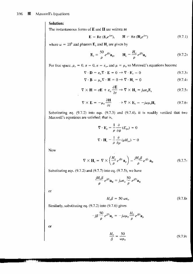
396 • Maxwell's Equations
Solution:
The instantaneous forms of E and H are written as
E = Re (EseJal), H = Re (Hse
J"')
where co = 106 and phasors Es and Hs are given by
50 HE = —' e^a H = — e^za
p *' p "For free space, pv = 0, a = 0, e = eo, and ft = fio so Maxwell's equations become
V-B = |ioV-H = 0-> V-Ha: = 0
dE
dt> V X H S = j
•iii
V X E = -fio —
(9.7.1)
(9.7.2)
(9.7.3)
(9.7.4)
(9.7.5)
(9.7.6)
Substituting eq. (9.7.2) into eqs. (9.7.3) and (9.7.4), it is readily verified that twoMaxwell's equations are satisfied; that is,
Now
V X Hs = V XP V P
Substituting eqs. (9.7.2) and (9.7.7) into eq. (9.7.5), we have
JHOI3 mz . 50 M,
(9.7.7i
or
//o/3 = 50 a)eo
Similarly, substituting eq. (9.7.2) into (9.7.6) gives
P
or
(9.7.8)
(9.7.9)
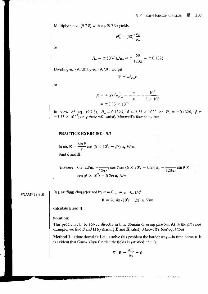
9.7 TIME-HARMONIC FIELDS 397
Multiplying eq. (9.7.8) with eq. (9.7.9) yields
or
Mo
50Ho = ±50V sJno = ± 7 ^ " = ± 0 - 1 3 2 6
Dividing eq. (9.7.8) by eq. (9.7.9), we get
I32 = o;2/x0e0
or
0 = ± aVp,
= ±3.33 X 10
10"
3 X 10s
- 3
In view of eq. (9.7.8), Ho = 0.1326, & = 3.33 X 10~3 or Ho = -0.1326, j3 =— 3.33 X 10~3; only these will satisfy Maxwell's four equations.
PRACTICE EXERCISE 9.7
In air, E = ^— cos (6 X 10⁷r - /3r) a* V/m.r
Find j3 and H.
Answer: 0.2 rad/m, r cos 6 sin (6 X 10⁷? - 0.2r) ar — sin S Xllzr2 1207rr
cos (6 X 10⁷f - 0.2r) % A/m.
EXAMPLE 9.8In a medium characterized by a = 0, \x = /xo, eo, and
E = 20 sin (108f - j3z) a7 V/m
calculate /8 and H.
Solution:
This problem can be solved directly in time domain or using phasors. As in the previousexample, we find 13 and H by making E and H satisfy Maxwell's four equations.
Method 1 (time domain): Let us solve this problem the harder way—in time domain. Itis evident that Gauss's law for electric fields is satisfied; that is,
dy

398 • Maxwell's Equations
From Faraday's law,
V X E = - /
But
V X E =
dHdt
A A Adx dy dz0 Ey 0
H = - - I (V X E)dt
dEy dEy
dz dx
Hence,
= 20/3 cos (108f - (3z) ax + 0
H = cos (108r - pz) dtax
^ s i - I3z)ax (9.8.1)
It is readily verified that
dx
showing that Gauss's law for magnetic fields is satisfied. Lastly, from Ampere's law
V X H = CTE + £1
E = - | (V X H) (9.8.2)
because a = 0.But
V X H =A A Adx dy dzHr 0 0
dHx dHx
cos(108? - $z)ay + 0
where H in eq. (9.8.1) has been substituted. Thus eq. (9.8.2) becomes
20/S2
E = cos(10 8r- (3z)dtay
2O/32
•sin(108f -
Comparing this with the given E, we have
= 20
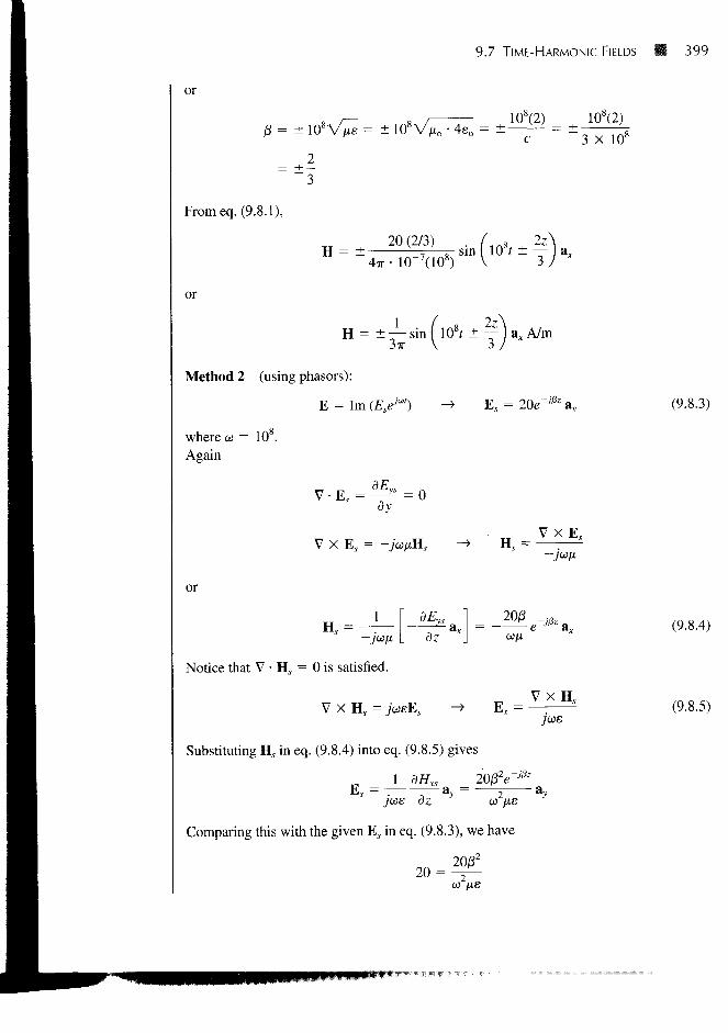
9.7 TIME-HARMONIC FIELDS • 399
or
= ± 108Vtis = ± 10SVIXO • 4eo = ±108(2) 108(2)
3 X 10B
From eq. (9.8.1),
or
1 / 2z\H = ± — sin 108?±— axA/m
3TT V 3/
Method 2 (using phasors):
E = Im ( £ y ) -> E, = av
where co =Again
10°.
V X E, =
dy
• -> " H, =V X Es
or
20/3 fr
Notice that V • H, = 0 is satisfied.
V X Hs = ji E, =V X H,
jus
Substituting H^ in eq. (9.8.4) into eq. (9.8.5) gives
2co /xe
Comparing this with the given Es in eq. (9.8.3), we have
^co /xe
(9.8.3)
(9.8.4)
(9.8.5)

400 Maxwell's Equations
or
as obtained before. From eq. (9.8.4),
„ ^ 2 0 ( 2 / 3 ) ^
10 8 (4T X 10 ') 3TT
H = Im (H/" 1 )
= ± — sin (108f ± Qz) ax A/m3TT
as obtained before. It should be noticed that working with phasors provides a considerablesimplification compared with working directly in time domain. Also, notice that we haveused
A = Im (Asejat)
because the given E is in sine form and not cosine. We could have used
A = Re (Asejo")
in which case sine is expressed in terms of cosine and eq. (9.8.3) would be
E = 20 cos (108? - & - 90°) av = Re (EseM)
or
and we follow the same procedure.
PRACTICE EXERCISE 9.8
A medium is characterized by a = 0, n = 2/*,, and s = 5eo. If H = 2cos {(jit — 3y) a_, A/m, calculate us and E.
Answer: 2.846 X l(f rad/s, -476.8 cos (2.846 X 10⁸f - 3v) a, V/m.
SUMMARY 1. In this chapter, we have introduced two fundamental concepts: electromotive force(emf), based on Faraday's experiments, and displacement current, which resulted fromMaxwell's hypothesis. These concepts call for modifications in Maxwell's curl equa-tions obtained for static EM fields to accommodate the time dependence of the fields.
2. Faraday's law states that the induced emf is given by (N = 1)
dt