Review P-values

Type I and Type II Errors

Talk to your kids about p-value, or someone else will.

p-value: If H0 is true, what would the chances of observing as

much evidence as we did?

If the p-value is small, then the observed statistic is very

unlikely under the null hypothesis.

Smaller p-values stronger evidence against the null.

Example: We suspect that a coin is unfair (the proportion of

times it comes up heads is not .50)

π is the proportion of flips that come up heads.

Scenario 1: We flip the coin 10 times and get 5 heads.

There is no way to get less evidence against H0, the sample

proportion is right on .50.

The p-value is….

A) 0

B) 0.05

C) 1

D) Impossible to tell

Scenario 1: We flip the coin 10 times and get 5 heads.

There is no way to get less evidence against H0, the sample

proportion is right on .50.

The p-value is….

C) 1

There p-value is 1 because any sample would have as much

evidence against H0 or more.

Area that’s 0 heads or more from 5 heads out of 10: 1.000

Scenario 2: We get 4 heads out of 10.

It’s not exactly .50, so there is some evidence against the null

hypothesis, but it isn’t significant.

The p-value is….

A) 0

B) Small ( less than 0.05)

C) Large (more than 0.05)

D) Impossible to tell

Scenario 2: We get 4 heads out of 10.

It’s not exactly .50, so there is some evidence against the null

hypothesis, but it isn’t significant.

The p-value is….

C) Large, p = 0.754 in fact

Getting at least one head more or less than 5/10 is common,

even with a fair coin. It happens .754 of the time, so the

p-value is 0.754.

Area that’s 1 head or more away from 5 out of 10: 0.754.

Scenario 3: 9 heads out of 10 flips.

This time, the sample proportion is .90 or 9/10. It’s far from

the null hypothesis value of .50, so the p-value is going to be

small.

It’s possible that a fair coin comes up with 9 heads in 10 flips,

but it’s unlikely. Getting 4 or more heads away from 5/10 only

happens .021 of the time, so that’s our p-value.

p-value = 0.021.

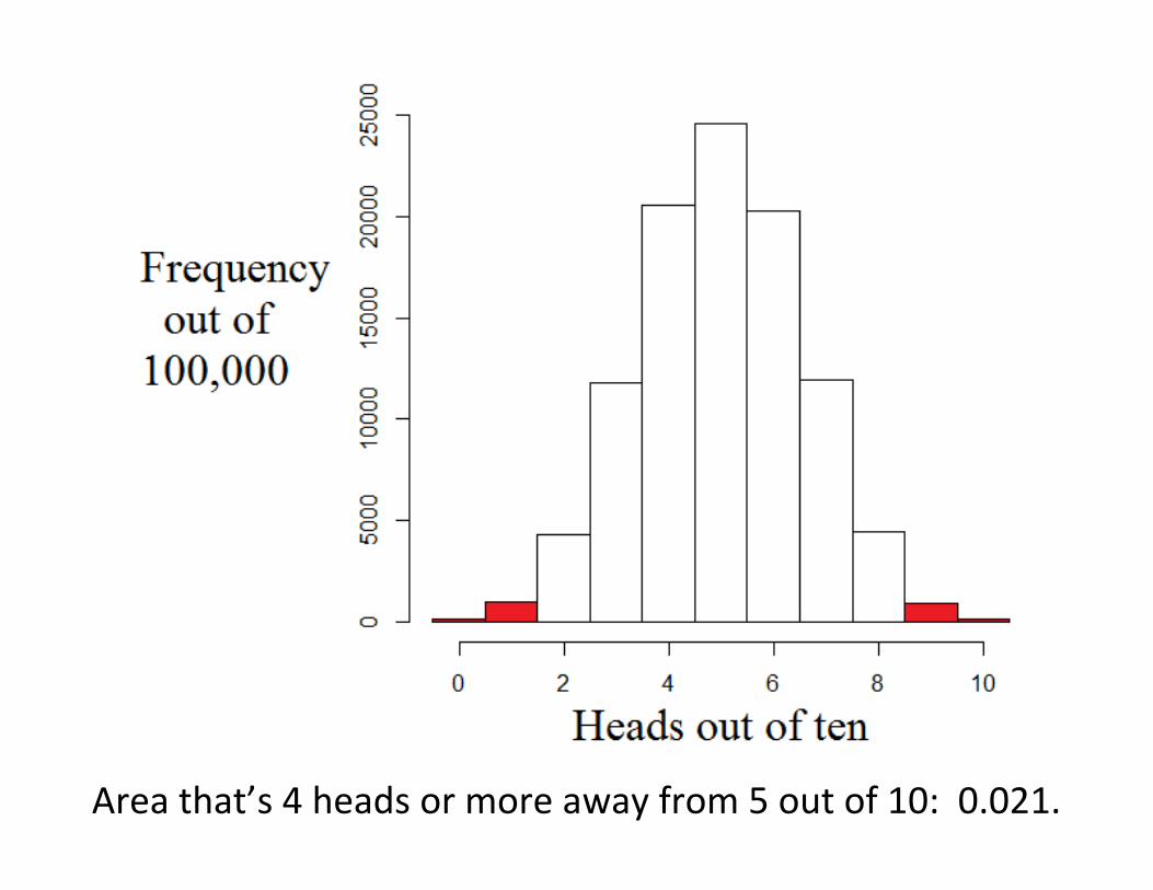
Area that’s 4 heads or more away from 5 out of 10: 0.021.

Getting 9 heads out of 10 is so unlikely for a fair coin that it we

might start to doubt the coin is fair at all.

Using the standard α = 0.05 we could reject the

assumption that the coin is fair.

Because p-value < α we reject the null hypothesis and

conclude the coin is not fair.

I hope this isn’t too repetitive.

But what is α?

Alpha is the chance we’re willing to take of rejecting the null

hypothesis even when it’s true.

When we get nine heads out of ten, the chance of that

happening if H0 is true is less the acceptable chance of falsely

rejecting, so we take that chance.

Rejecting the null when it’s true is called making a Type 1

error. That means…

α is the type 1 error rate.

α is the rate that type 1 errors will occur. That means if we’re

testing many hypotheses at once, then α of rejected nulls will

be falsely rejected.

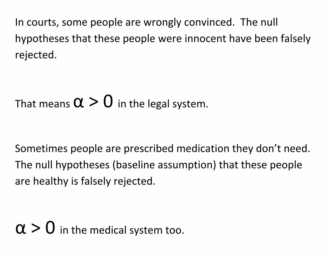
In courts, some people are wrongly convinced. The null

hypotheses that these people were innocent have been falsely

rejected.

That means α > 0 in the legal system.

Sometimes people are prescribed medication they don’t need.

The null hypotheses (baseline assumption) that these people

are healthy is falsely rejected.

α > 0 in the medical system too.

If there’s a type 1 error, is there a type 2 error?

Type 2 error: The act of failing to reject the null when it is

false.

β is the type 2 error rate.

β is the chance of failing to reject the null hypothesis when we

should reject it.

A type 1 error is falsely leaping to a conclusion.

A type 1 error is falsely leaping to a conclusion.

A type 2 error is failing to come to a conclusion that you should

have.

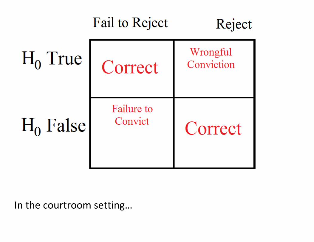
In the courtroom setting…

β depends on additional factors from your sample, like the

standard error and the effect size.

Effect size is the raw distance from the null hypothesis you’re

considering when you set the type II error rate.

In the coin flipping scenarios, the farther we got from 5 heads

out of 10, the larger the effect size.

β decreases when effect size increases.

If a new medicine causes someone’s heart to explode (large

effect size), that’s easier to notice than a small increase in

blood presure (small effect size).

1 – β is called the power of the test. If we’re considering

a large effect, our test is going to have a lot of power to

detect the effect and reject the null based on that.

β increases when standard error increases.

The less random noise/variation, the better.

If the medicine causes EXACTLY the same increase in blood

pressure (no standard error), that will be easier to detect than

a change in pressue that’s got a lot of randomness (large

standard error)

Having a bigger sample size helps by making the standard error

smaller.

Since we won’t know the effect size or the standard error until

we see the data, there’s not usually a way to set β, the type 2

error rate, before data collection like you can with α, the type

1 error rate.

Also, computing power is a mess,we won’t deal with the

numerical details, only its trends.

β increases with standard error, and

decreases with effect size.

Also, β decreases when α increases. There’s an important tradeoff. We can’t usually get a small

type 1 error rate and a small type 2 error rate at the same

time.

When we make α small, we’re less likely to reject the null.

That means we’re more likely to fail to reject the null.

Failing to reject the null when we should is a type 2 error.

Often it comes down to which mistake would you rather

make? If you’re setting a critical value (like a critical t-score),

the tradeoff is what you should be considering.

Should you cross the street or not?

Does this person need medicine or not?

Having more information in the form of a bigger sample (larger

n) means fewer mistakes of either type, but bigger samples are

more expensive.

Back to piling on examples!

Example: Should you take your vitamins?

You’re worried about getting sick and you’re trying to

determine if you should take a vitamin pill to get better faster.

The null hypothesis is that you’re healthy enough not to need a

vitamin pill. The alternative is a vitamin pill will help.

What’s the best set of type 1 and type 2 error rates?

H0: Healthy enough to not need vitamins.

HA: Sick enough that vitamins will help.

What’s the best set of type 1 and type 2 error rates?

α = .20 , β = .11

α = .05 , β = .24

α = .01 , β = .56

Pick the one with the small type 2 error rate.

α = .20 , β = .11

A type 1 error would be to waste a vitamin pill when you

weren’t getting sick.

A type 2 error would be to not take the vitamin pill and get sick

when you could have avoided it.

Making a type 2 error is a bigger problem, so we try to keep

the type 2 error small.

Assume you have a really high-tech bathroom scale. It

measures your health and tells it to you as a single value.

Having 40 health is good, having less than 40 health means

you’re sick. Having more than 40 is not big deal.

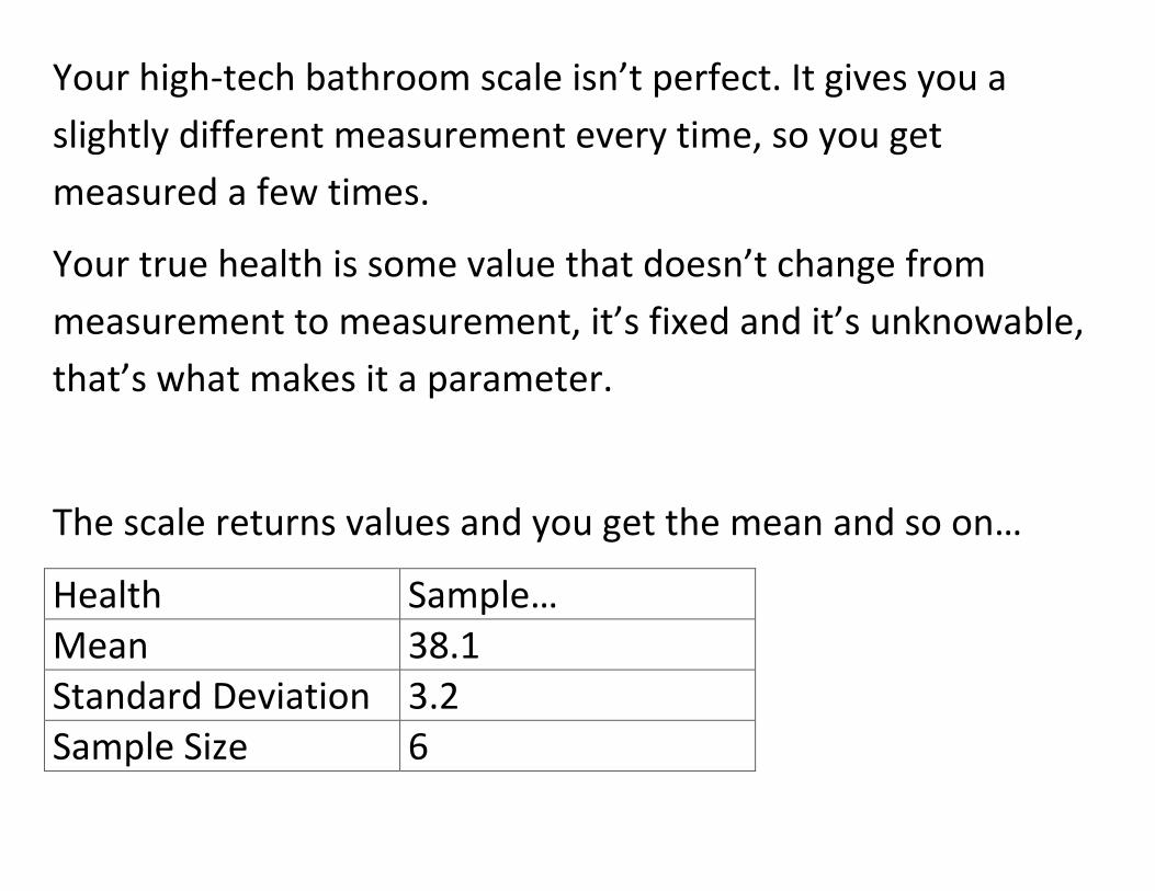
Your high-tech bathroom scale isn’t perfect. It gives you a

slightly different measurement every time, so you get

measured a few times.

Your true health is some value that doesn’t change from

measurement to measurement, it’s fixed and it’s unknowable,

that’s what makes it a parameter.

The scale returns values and you get the mean and so on…

Health Sample… Mean 38.1 Standard Deviation 3.2 Sample Size 6

What do you do with this information.

Start by indentifying:

Is this a one-sample or two-sample test?

Is this a one-tailed/sided or two-tailed test?

Start by indentifying:

Is this a one-sample or two-sample test? ONE

Is this a one-tailed/sided or two-tailed test? ONE

From SPSS, you get the value under “sig. (2-tailed)” of

.2066

What do you do with this?

From SPSS, you get the value under “sig. (2-tailed)” of

.2066

It’s a one-tailed test, the SPSS significiance is cut in half

because we’re only concerned with one tail.

(Cut in half only applies if sample mean less than 40. If health

was more than 40 we would fail to reject because your scale

would tell you you’re even healthier than you have to be.)

p-value = .1033, less than alpha = 0.20, so we reject.

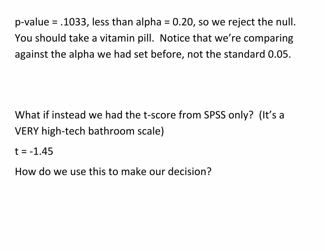
p-value = .1033, less than alpha = 0.20, so we reject the null.

You should take a vitamin pill. Notice that we’re comparing

against the alpha we had set before, not the standard 0.05.

What if instead we had the t-score from SPSS only? (It’s a

VERY high-tech bathroom scale)

t = -1.45

How do we use this to make our decision?

t= -1.45

Compare to the critical value, or t*

The degrees of freedom is n-1 = 5

The t*, in the one-sided table for alpha = 0.20 is t* = 0.919.

(We’re using a significance level so large, it’s not on your table,

t* from computer)

Ignoring the negative, t-score = 1.45 > critical value of 0.919

Reject the null.

What if all you have is the 80% confidence interval of your

health? (Null hypothesis: Health = 40)

[ 36.5 to 39.7]

What do we get from that?

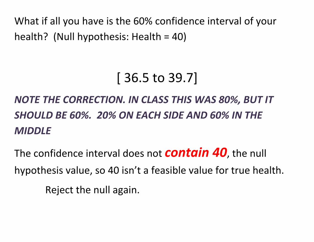
What if all you have is the 60% confidence interval of your

health? (Null hypothesis: Health = 40)

[ 36.5 to 39.7]

NOTE THE CORRECTION. IN CLASS THIS WAS 80%, BUT IT

SHOULD BE 60%. 20% ON EACH SIDE AND 60% IN THE

MIDDLE

The confidence interval does not contain 40, the null

hypothesis value, so 40 isn’t a feasible value for true health.

Reject the null again.

Three ways to determine if a mean is significantly

different from a given value.

1. If the p-value is less than alpha, reject the null.

2. If the t-score is greater than the critical, reject the

null.

3. If the (1 – alpha) confidence interval does not

contain the hypothesized value, reject.

For interest topic: Multiple testing (if time permits)

Sometimes you’ll need to test many hypotheses together.

Example: To check that a new drug doesn’t have side effects,

we’d want to test that it doesn’t change…

blood pressure,

hours slept,

heart rate,

levels of various horomones…

Each of these aspects of the body needs its own hypothesis

test.

For interest topic: Multiple testing (if time permits)

Assume the drug doesn’t have any side effects

If we use α = 0.05 for each of those aspects then there’s

a 5% chance of finding a change in blood pressure, and

a 5% chance of finding a change in hours slept, and

a 5% chance of…

The chance of falsely concluding the drug has side effects is a

lot higher than 5% because those chances are all for different

things, they stack up.

For interest topic: Multiple testing (if time permits)

For testing four things at 5%, we’d reject one falsely 18.54% of

the time.

If we wanted the general null hypothesis that the drug has no

side effects to have a 5% type 1 error rate, we’d need a

multiple testing correction.

These corrections (Sidak, Bonferroni, etc.) reduce the alpha for

each test until there’s only a 5% chance of even a single false

rejection.

Next time: Wrap up any loose ends in chapter 7

Start chapter 10: Correlation