Review of Selected Surface Graphics Topics (1)

Jian Huang, CS 594, Spring 2002

Visible Light

3-Component Color

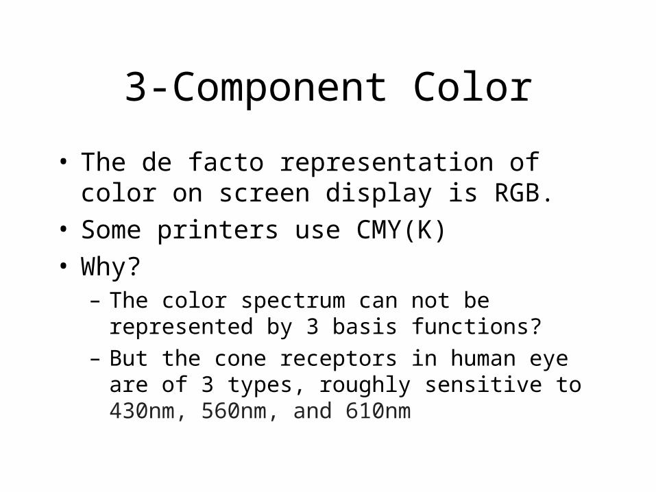
• The de facto representation of color on screen display is RGB.

• Some printers use CMY(K)• Why?

– The color spectrum can not be represented by 3 basis functions?

– But the cone receptors in human eye are of 3 types, roughly sensitive to 430nm, 560nm, and 610nm

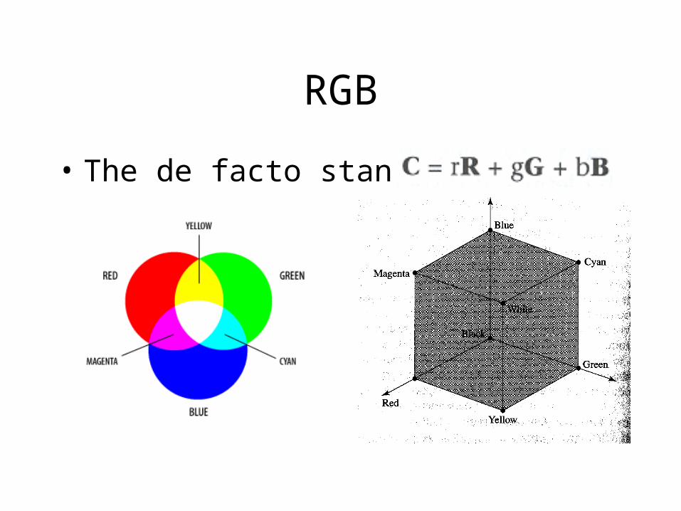
RGB

• The de facto standard

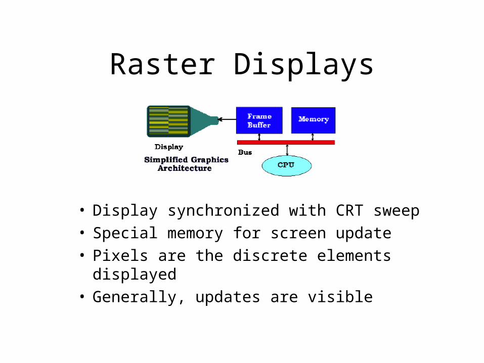
Raster Displays

• Display synchronized with CRT sweep• Special memory for screen update• Pixels are the discrete elements displayed• Generally, updates are visible

Polygon Mesh

• Set of surface polygons that enclose an object interior, polygon mesh

• De facto: triangles, triangle mesh.

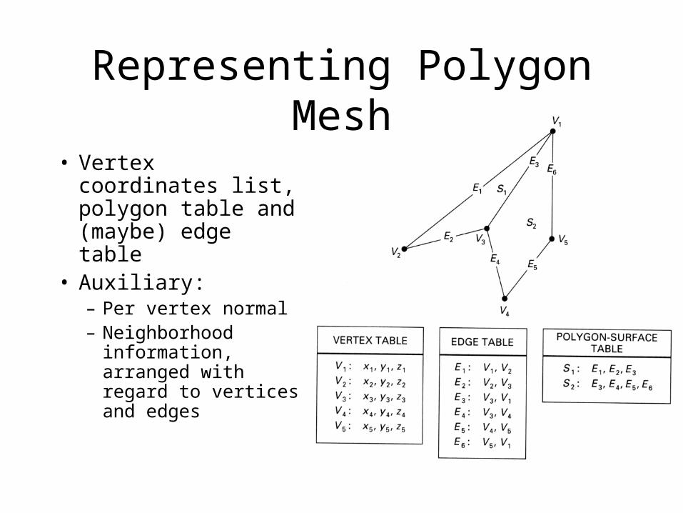
Representing Polygon Mesh

• Vertex coordinates list, polygon table and (maybe) edge table

• Auxiliary:– Per vertex normal– Neighborhood

information, arranged with regard to vertices and edges

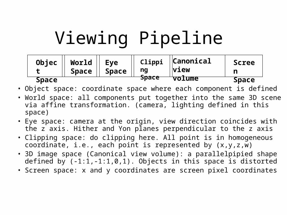
Viewing Pipeline

• Object space: coordinate space where each component is defined• World space: all components put together into the same 3D scene

via affine transformation. (camera, lighting defined in this space)• Eye space: camera at the origin, view direction coincides with the

z axis. Hither and Yon planes perpendicular to the z axis• Clipping space: do clipping here. All point is in homogeneous

coordinate, i.e., each point is represented by (x,y,z,w)• 3D image space (Canonical view volume): a parallelpipied shape

defined by (-1:1,-1:1,0,1). Objects in this space is distorted• Screen space: x and y coordinates are screen pixel coordinates

Object Space

World Space

Eye Space

Clipping Space

Canonical view volume

Screen Space

Spaces: ExampleObject Space and World Space:

Eye-Space:

eye

3.

Spaces: Example

Clip Space:

Image Space:

1. 2.

3. 4.

5. 6.

Homogeneous Coordinates

• Matrix/Vector format for translation:

Translation in Homogenous Coordinates

• There exists an inverse mapping for each function

• There exists an identity mapping

Why these properties are important

• when these conditions are shown for any class of functions it can be proven that such a class is closed under composition

• i. e. any series of translations can be composed to a

single translation.

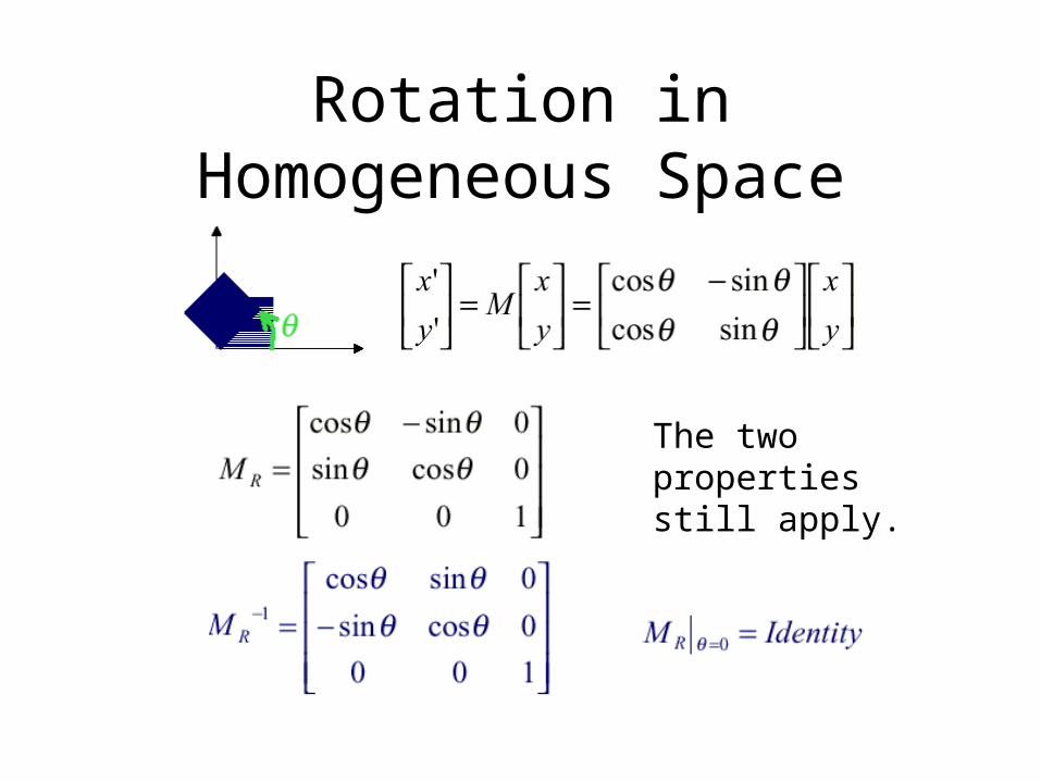
Rotation in Homogeneous Space

The two properties still apply.

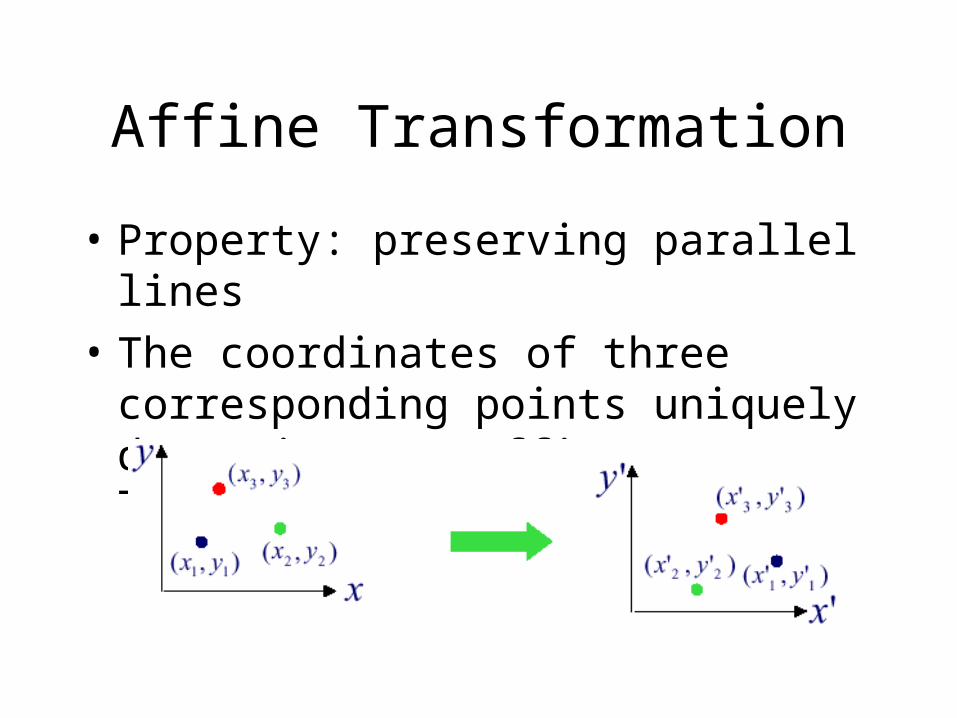
Affine Transformation

• Property: preserving parallel lines

• The coordinates of three corresponding points uniquely determine any Affine Transform!!

Affine Transformations

• Translation

• Rotation

• Scaling

• Shearing

T

Affine Transformation in 3D

• Translation

• Rotate

• Scale

• Shear

Viewing

• Object space to World space: affine transformation

• World space to Eye space: how?

• Eye space to Clipping space involves projection and viewing frustum

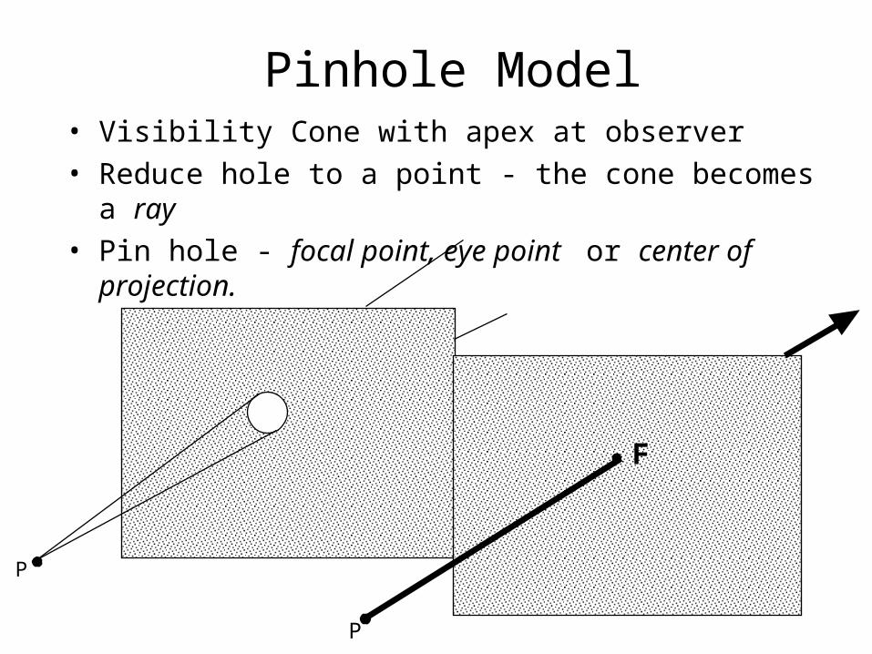
Pinhole Model• Visibility Cone with apex at observer• Reduce hole to a point - the cone becomes a ray• Pin hole - focal point, eye point or center of

projection.

P

P

F

Perspective Projectionand Pin Hole Camera

• Projection point sees anything on ray through pinhole F

• Point W projects along the ray through F to appear at I (intersection of WF with image plane)

F

Image

WorldI

W

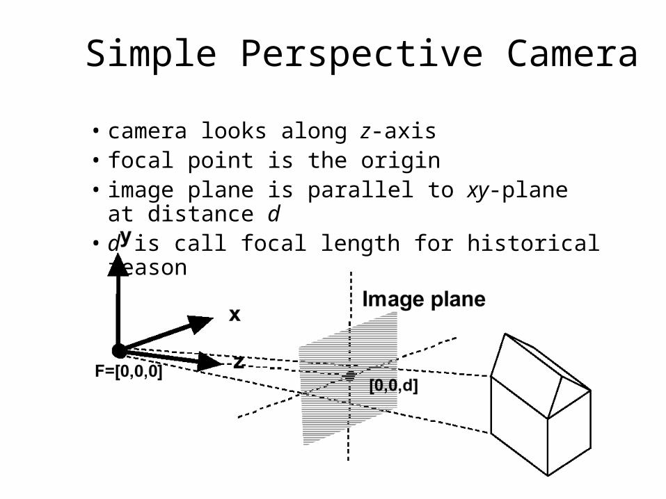
Simple Perspective Camera

• camera looks along z-axis• focal point is the origin• image plane is parallel to xy-plane at

distance d• d is call focal length for historical reason

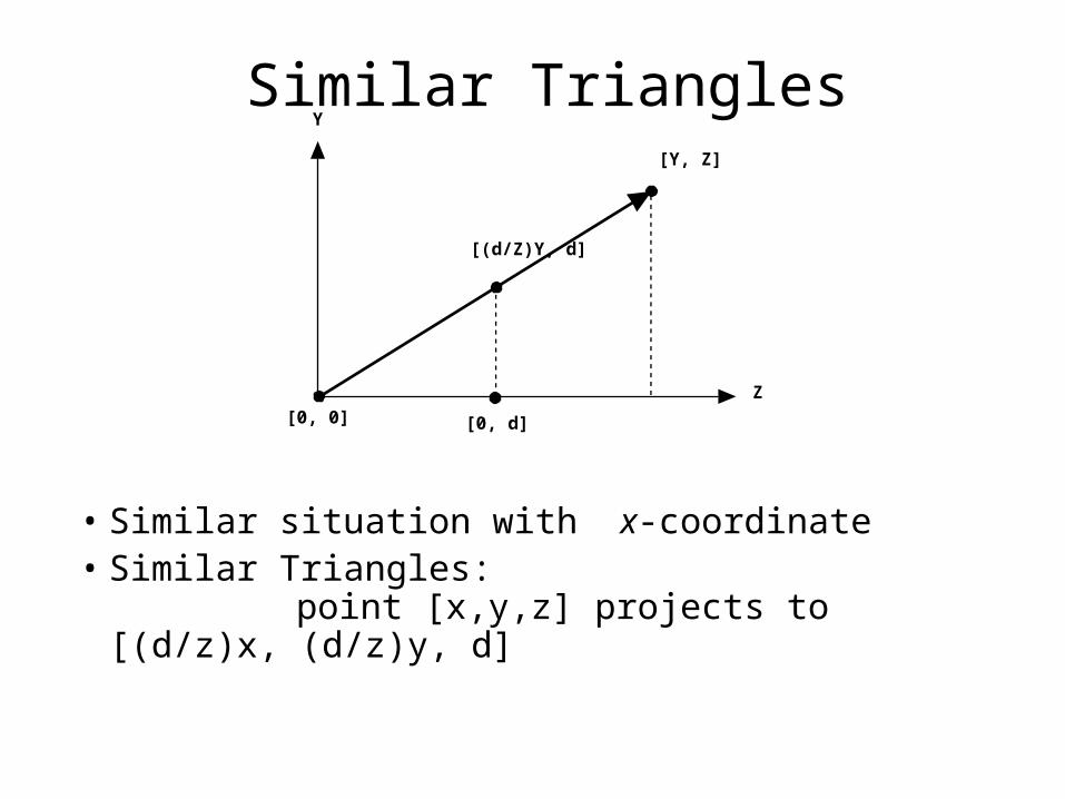
Similar TrianglesY

Z

[0, d][0, 0]

[Y, Z]

[(d/Z)Y, d]

• Similar situation with x-coordinate• Similar Triangles:

point [x,y,z] projects to [(d/z)x, (d/z)y, d]

View Volume

• Defines visible region of space, pyramid edges are clipping planes

• Frustum :truncated pyramid with near and far clipping planes

– Near (Hither) plane ? Don’t care about behind the camera

– Far (Yon) plane, define field of interest, allows z to be scaled to a limited fixed-point value for z-buffering.

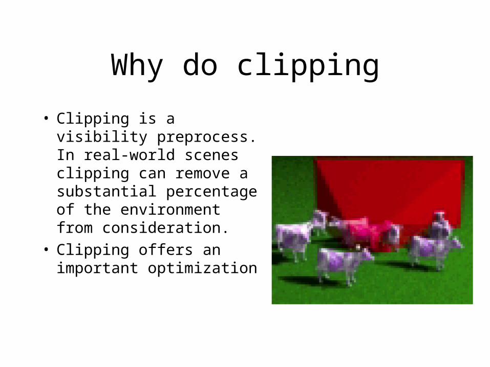
Why do clipping

• Clipping is a visibility preprocess. In real-world scenes clipping can remove a substantial percentage of the environment from consideration.

• Clipping offers an important optimization

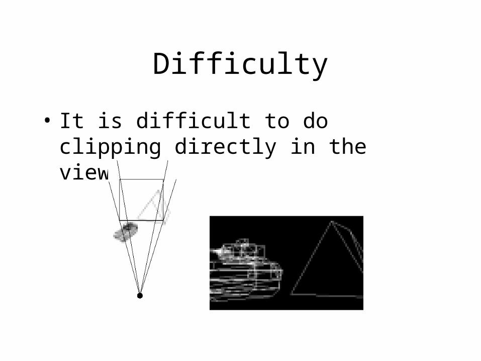
Difficulty

• It is difficult to do clipping directly in the viewing frustum

Canonical View Volume

• Normalize the viewing frustum to a cube, canonical view volume

• Converts perspective frustum to orthographic frustum – perspective transformation

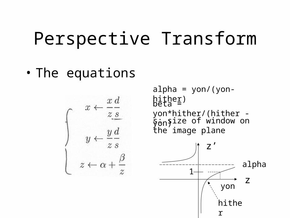
Perspective Transform

• The equationsalpha = yon/(yon-hither)

beta = yon*hither/(hither - yon)

s: size of window on the image plane

z

z’

1alpha

yon

hither

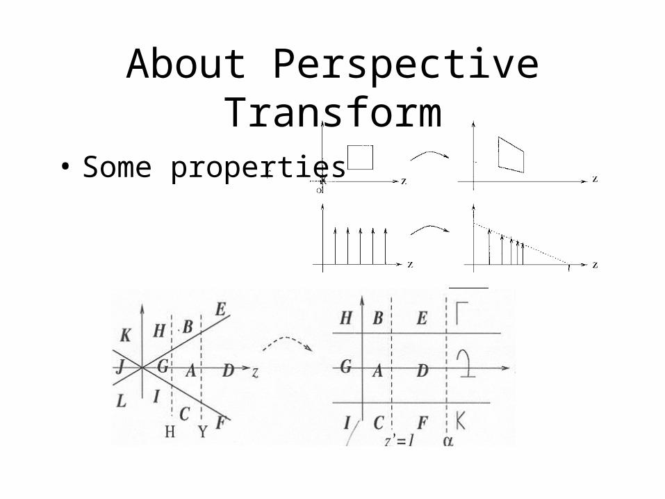
About Perspective Transform

• Some properties

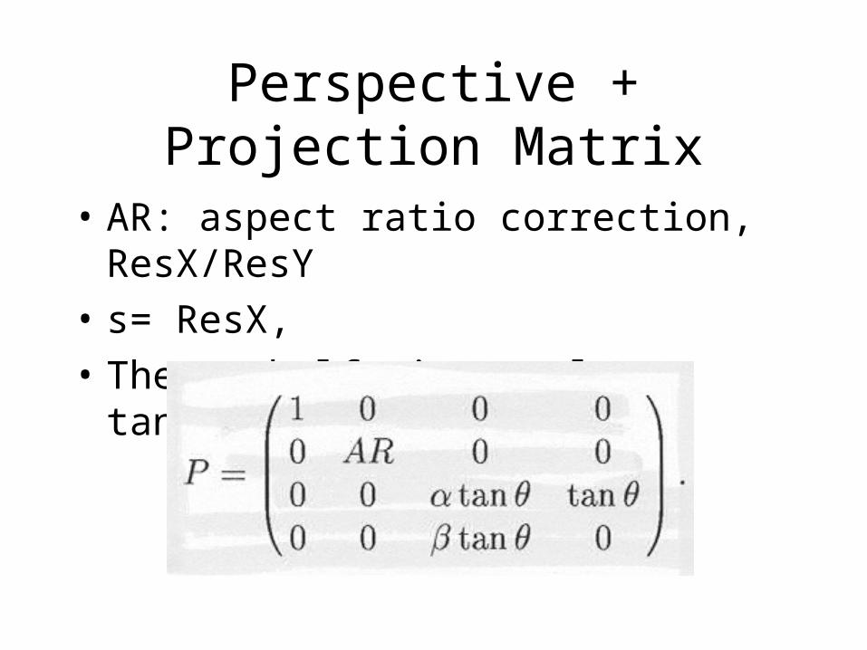
Perspective + Projection Matrix

• AR: aspect ratio correction, ResX/ResY

• s= ResX,

• Theta: half view angle, tan(theta) = s/d

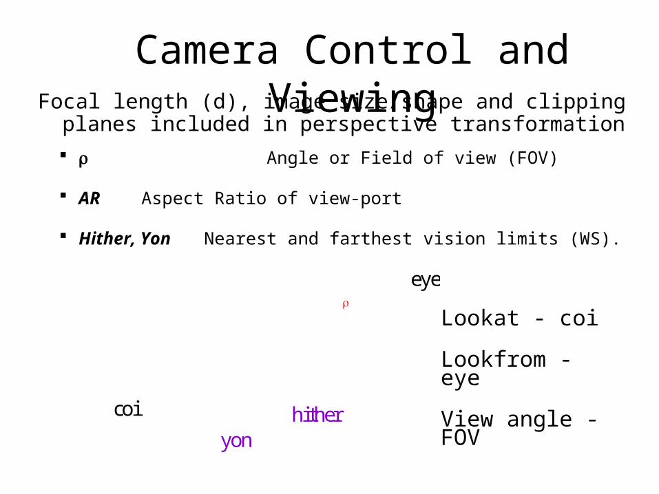
Camera Control and ViewingFocal length (d), image size/shape and clipping planes included in

perspective transformation

               Angle or Field of view (FOV)

AR       Aspect Ratio of view-port

Hither, Yon Nearest and farthest vision limits (WS).

eye

coi

hitheryon

Lookat - coi

Lookfrom - eye

View angle - FOV

Complete Perspective

• Specify near and far clipping planes - transform z between znear and zfar on to a fixed range

• Specify field-of-view (fov) angle• OpenGL’s glFrustum and gluPerspective do

these

More Viewing Parameters

Camera, Eye or Observer:lookfrom:location of focal point or cameralookat: point to be centered in image

Camera orientation about the lookat-lookfrom axis

vup: a vector that is pointing straight up in the image. This is like an

orientation.

Point Clipping

(x, y) is inside iff

Xmin Xmax

Ymin

Ymax

Xmin x Xmax Ymin y Ymax

AND

One Plane At a Time Clipping(a.k.a. Sutherland-Hodgeman Clipping)• The Sutherland-Hodgeman triangle clipping

algorithm uses a divide-and-conquer strategy. • Clip a triangle against a single plane. Each of the

clipping planes are applied in succession to every triangle.

• There is minimal storage requirements for this algorithm, and it is well suited to pipelining.

• It is often used in hardware implementations.

Sutherland-HodgmanPolygon Clipping Algorithm

Subproblem: clip a polygon (input: vertex list) against a

single clip edges output the vertex list(s) for the resulting

clipped polygon(s) Clip against all four planes

generalizes to 3D (6 planes) generalizes to any convex clip

polygon/polyhedron Used in viewing transforms

Polygon Clipping At Work

With Pictures

4DPolygonClip

Use Sutherland Hodgman algorithm

Use arrays for input and output lists

There are six planes of course !

4D Clipping• Point A is inside, Point B is outside. Clip edge AB

x = Ax + t(Bx – Ax)

y = Ay + t(By – Ay)

z = Az + t(Bz – Az)

w = Aw + t(Bw – Aw)

• Clip boundary: x/w = 1 i.e. (x–w=0); w-x = Aw – Ax + t(Bw – Aw – Bx + Ax) = 0

Solve for t.

Why Homogeneous Clipping• Efficiency/Uniformity: A single clip procedure is

typically provided in hardware, optimized for canonical view volume.

• The perspective projection canonical view volume can be transformed into a parallel-projection view volume, so the same clipping procedure can be used.

• But for this, clipping must be done in homogenous coordinates (and not in 3D). Some transformations can result in negative W : 3D clipping would not work.

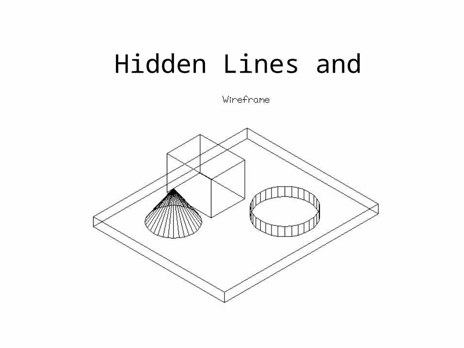
Hidden Lines and Surfaces

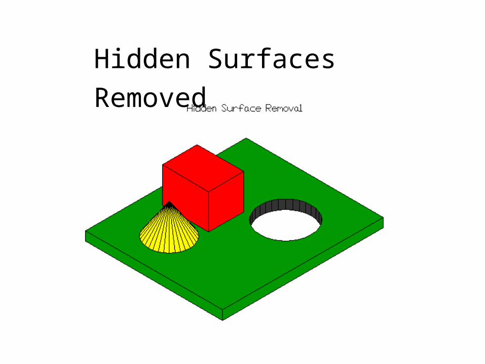
Hidden Surfaces Removed

Where Are We ?Canonical view volume (3D image space)

Clipping done

division by w

z > 0

x

y

znear far

clipped line

1

11

0

x

y

z

image plane

near far

clipped line

Painters AlgorithmSort objects in depth order

Draw all from Back-to-Front (far-to-near)

Is it so simple?

at z = 22, at z = 18, at z = 10,

1 2 3

X

Y

3D CyclesHow do we deal with cycles?

Deal with intersections

How do we sort objects that overlap in Z?

Z

Form of the Input

Object types: what kind of objects does it handle?

convex vs. non-convex

polygons vs. everything else - smooth curves, non-continuous surfaces, volumetric data

Object Space

Geometry in, geometry out

Independent of image resolution

Followed by scan conversion

Form of the output

Image Space

Geometry in, image out

Visibility only at pixels

Precision: image/object space?

Object Space Algorithms

Volume testing – Weiler-Atherton, etc.

input: convex polygons + infinite eye pt

output: visible portions of wireframe edges

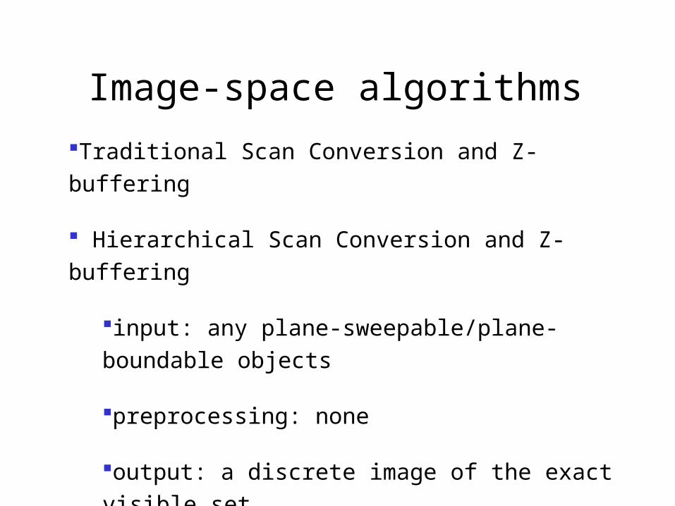
Image-space algorithms

Traditional Scan Conversion and Z-buffering

Hierarchical Scan Conversion and Z-buffering

input: any plane-sweepable/plane-boundable objects

preprocessing: none

output: a discrete image of the exact visible set

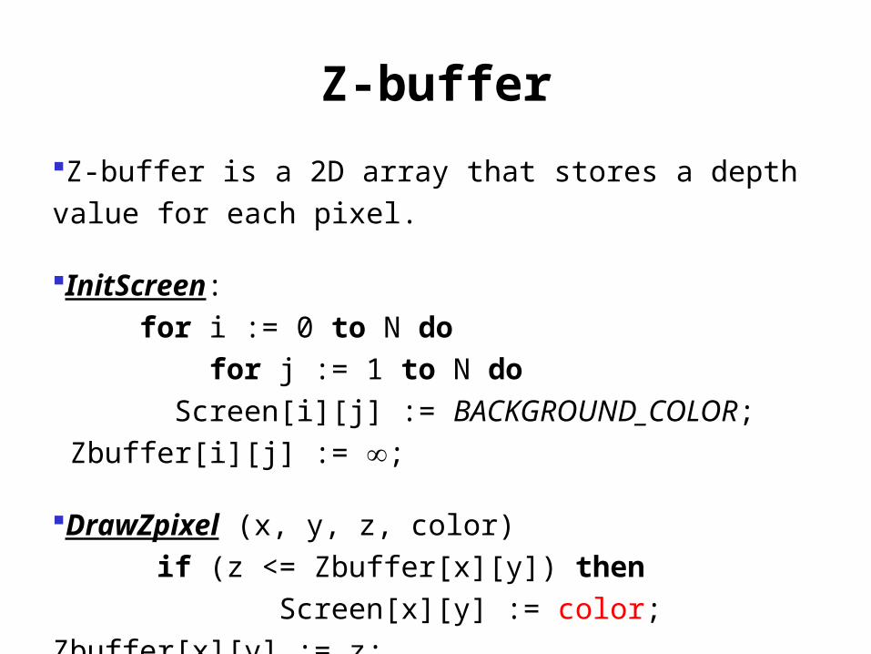
Z-buffer

Z-buffer is a 2D array that stores a depth value for each pixel.

InitScreen:

    for i := 0 to N do

        for j := 1 to N do

       Screen[i][j] := BACKGROUND_COLOR;  Zbuffer[i][j] := ;

DrawZpixel (x, y, z, color)

      if (z <= Zbuffer[x][y]) then

             Screen[x][y] := color; Zbuffer[x][y] := z;

Z-buffer: Scanline

I.  for each polygon do        for each pixel (x,y) in the polygon’s projection do             z := -(D+A*x+B*y)/C;             DrawZpixel(x, y, z, polygon’s color);

II.  for each scan-line y do        for each “in range” polygon projection do             for each pair (x1, x2) of X-intersections do                   for x := x1 to x2 do                         z := -(D+A*x+B*y)/C;                         DrawZpixel(x, y, z, polygon’s color);

If we know zx,y at (x,y) than:    zx+1,y = zx,y - A/C

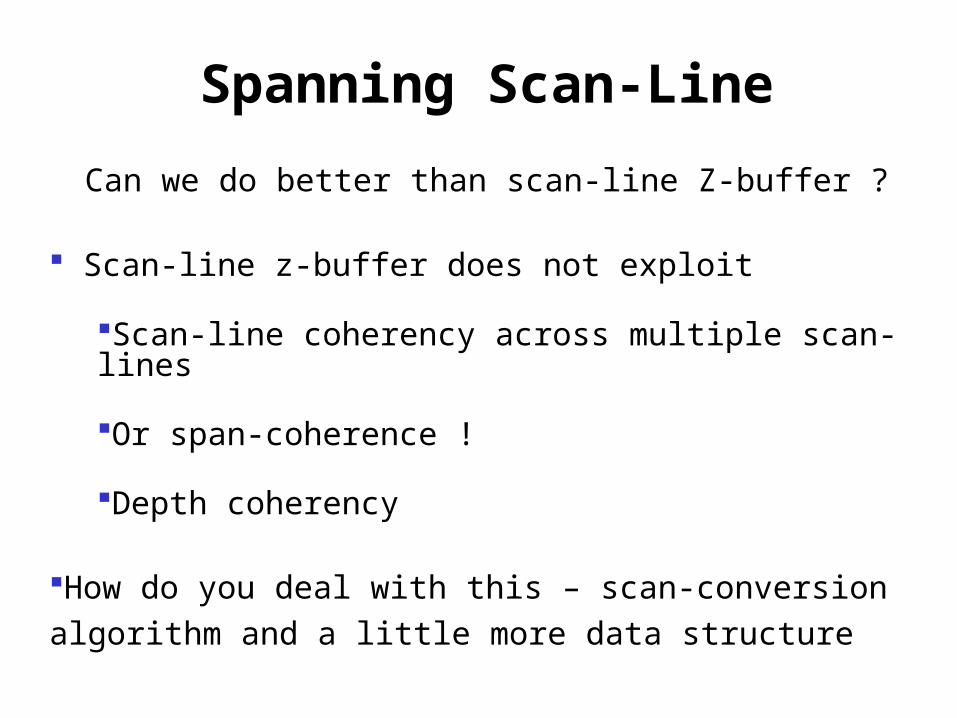
Spanning Scan-Line

Can we do better than scan-line Z-buffer ?

Scan-line z-buffer does not exploit

Scan-line coherency across multiple scan-lines

Or span-coherence !

Depth coherency

How do you deal with this – scan-conversion algorithm and a little

more data structure

Spanning Scan Line Algorithm

• Use no z-buffer• Each scan line is subdivided into

several "spans"• Determine which polygon the

current span belongs to• Shade the span using the current

polygon’s color• Exploit "span coherence" :• For each span, only one visibility

test needs to be done

surround intersect contained disjoint

Area Subdivision 1

(Warnock’s Algorithm)Divide and conquer: the relationship of a display area and a polygon after projection is one of the four basic cases:

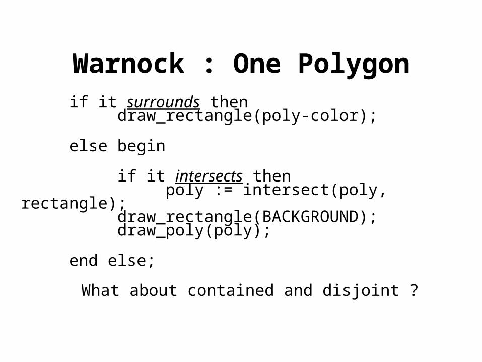
Warnock : One Polygonif it surrounds then

draw_rectangle(poly-color);

else begin

if it intersects thenpoly := intersect(poly, rectangle);

draw_rectangle(BACKGROUND);draw_poly(poly);

end else;

What about contained and disjoint ?

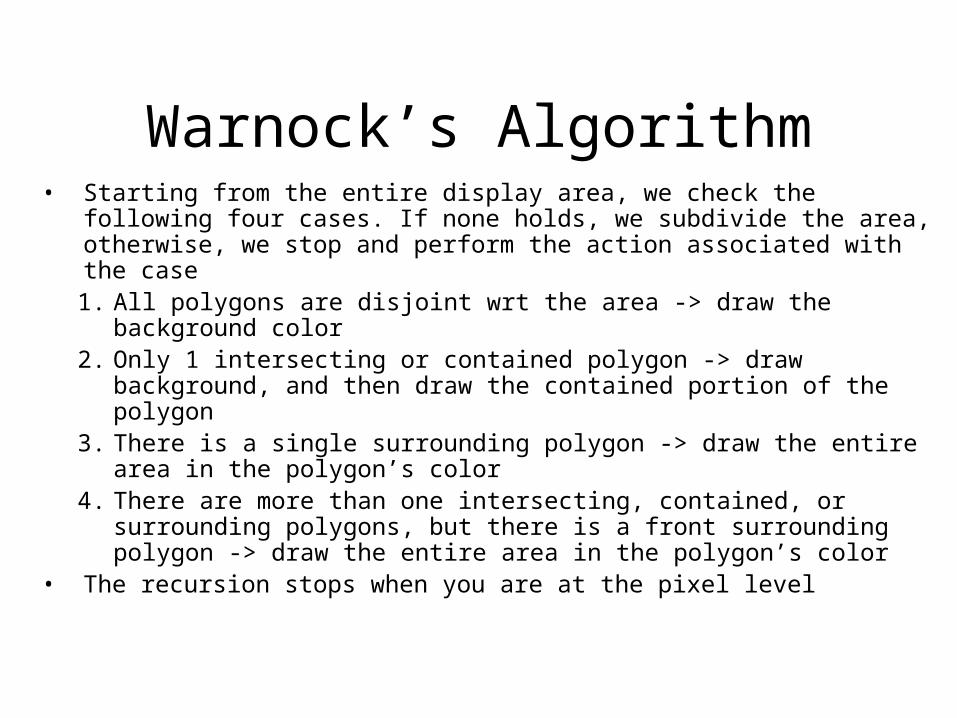
Warnock’s Algorithm• Starting from the entire display area, we check the following four

cases. If none holds, we subdivide the area, otherwise, we stop and perform the action associated with the case1. All polygons are disjoint wrt the area -> draw the background

color2. Only 1 intersecting or contained polygon -> draw background,

and then draw the contained portion of the polygon3. There is a single surrounding polygon -> draw the entire area in

the polygon’s color4. There are more than one intersecting, contained, or surrounding

polygons, but there is a front surrounding polygon -> draw the entire area in the polygon’s color

• The recursion stops when you are at the pixel level

At Single Pixel Level

• When the recursion stop and none of the four cases hold, we need to perform depth sort and draw the polygon with the closest Z value

• The algorithm is done at the object space level, except scan conversion and clipping are done at the image space level

Area Subdivision 2

Weiler -Atherton Algorithm

Object space

Like Warnock

Output – polygons of arbitrary accuracy

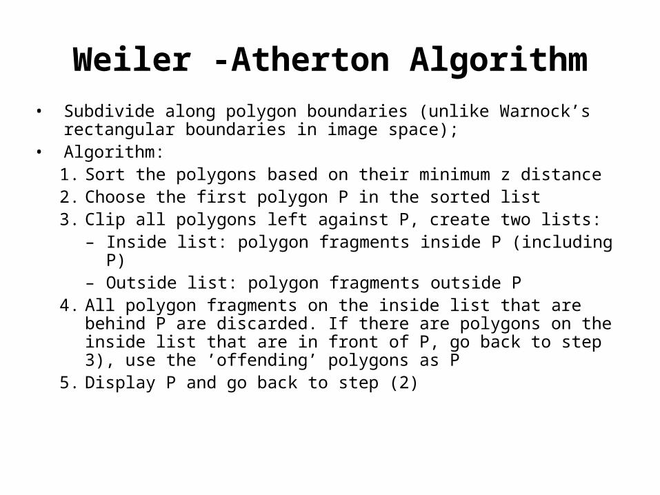
Weiler -Atherton Algorithm

• Subdivide along polygon boundaries (unlike Warnock’s rectangular boundaries in image space);

• Algorithm: 1. Sort the polygons based on their minimum z distance2. Choose the first polygon P in the sorted list 3. Clip all polygons left against P, create two lists:

– Inside list: polygon fragments inside P (including P)– Outside list: polygon fragments outside P

4. All polygon fragments on the inside list that are behind P are discarded. If there are polygons on the inside list that are in front of P, go back to step 3), use the ’offending’ polygons as P

5. Display P and go back to step (2)

tr

tr

1 32

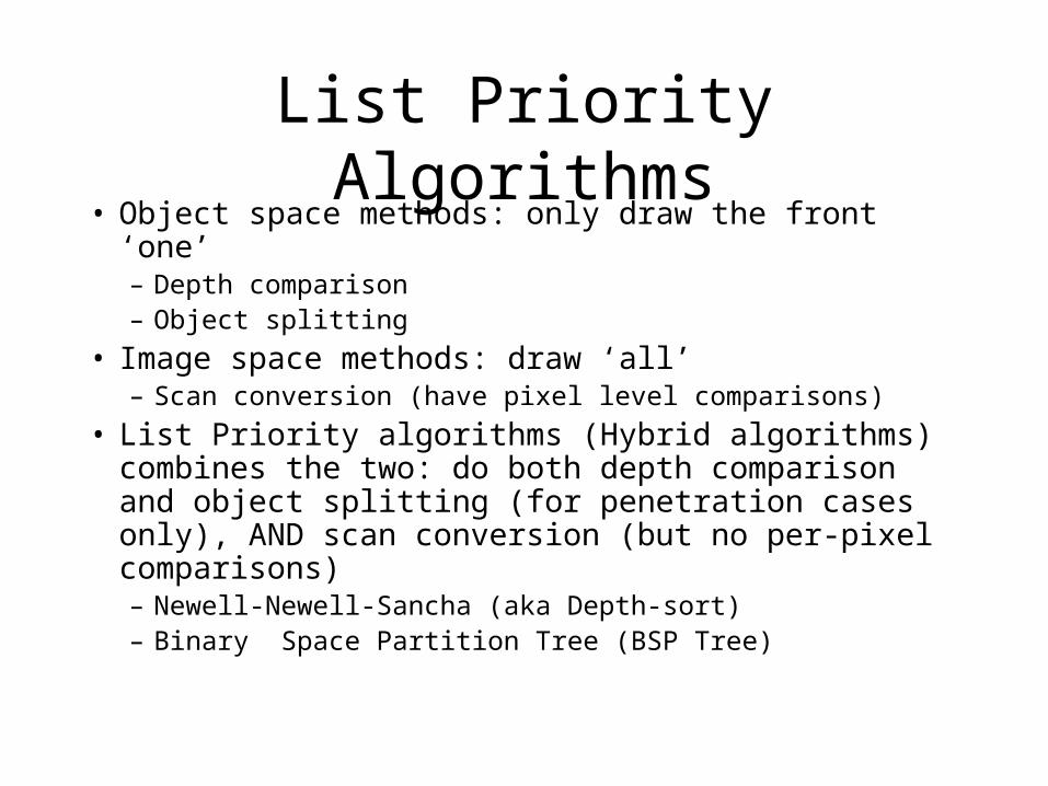
List Priority Algorithms• Object space methods: only draw the front ‘one’

– Depth comparison– Object splitting

• Image space methods: draw ‘all’– Scan conversion (have pixel level comparisons)

• List Priority algorithms (Hybrid algorithms) combines the two: do both depth comparison and object splitting (for penetration cases only), AND scan conversion (but no per-pixel comparisons)– Newell-Newell-Sancha (aka Depth-sort)– Binary Space Partition Tree (BSP Tree)

List Priority Algorithms

If objects do not overlap in X or in Y there is no need for hidden object removal process.

If they do not overlap in the Z dimension they can be sorted by Z and rendered in back (highest priority)-to-front (lowest priority) order (Painter’s Algorithm).

It is easy then to implement transparency.

How do we sort ? – different algorithms differ

Binary Space-Partitioning Tree

Given a polygon p

Two lists of polygons:

those that are behind(p) :B

those that are infront(p) :F

If eye is infornt(p), right display order is B, p,

Otherwise it is F, p, B

B p F

p

B F

back front

Bf Bb

p

F

Bb Bf

B

B p F

p

B F

back front

Bf Bb

p

F

Bb Bf

B

Display a BSP Tree

struct bspnode { p: Polygon; back, front : *bspnode;

} BSPTree;

BSP_display ( bspt )BSPTree *bspt;{ if (!bspt) return;

if (EyeInfrontPoly( bspt->p )) { BSP_display(bspt->back);Poly_display(bspt->p); BSP_display(bspt->front);} else {

BSP_display(bspt->front); Poly_display(bspt->p);BSP_display(bspt->back);

}}

Generating a BSP Tree

if (polys is empty ) then return NULL;rootp := first polygon in polys;

for each polygon p in the rest of polys doif p is infront of rootp then

add p to the front listelse if p is in the back of rootp then

add p to the back listelse split p into a back poly pb and front poly pf add pf to the front list add pb to the back list

end_for;bspt->back := BSP_gentree(back list);bspt->front := BSP_gentree(front list);bspt->p = rootp;return bspt;

3

4, 5b1

23

4

5

a b

1 5a

3

1

23

4

5

a b

1 5a

3

1, 2, 5a 4, 5b1

23

4

5

a b

2

2

5b

4