review of reliability theory, analytical techniques, and basic

Appendix

Review of Reliability Theory, Analytical Techniques,

and Basic Statistics

This appendix reviews the reliability theory, analytical modeling techniques, and statistical techniques commonly used in software reliability engineering studies. Reliability theory establishes a foundation for the application of reliability concepts and reliability-related quantities to a system. Analytical modeling provides frameworks for abstracting the information obtained from measurement-based studies. Statistical techniques allow us to extract reliability measures from data, analyze the structure of data, and test hypotheses. These techniques are useful in every phase of the empirical evaluation of software reliability. The reliability theory reviewed in this appendix includes reliability definitions, underlying mathematics, and failure rate functions. The analytical methods consist of combinatorial models, Markov models, Markov reward analysis, birth-death processes, and Poisson processes. The statistical techniques cover parameter estimation, characterization of empirical distribution, and multivariate analysis. Our discussion is not intended to be comprehensive. For a comprehensive study of the techniques, you are encouraged to read [Dani79, DeGr86, Dill84, Hogg83, Howa71, John82, Kend77, Mood74, Shoo83, Triv821.

B.1 Notation and Terminology

This section gives notation, terminology, and several important distributions that are referred to throughout App. B. The set of all possible outcomes of an experiment is called a sample space. A sample space can be made up of all kinds of things. For example, conducting an experi-

747

748 Appendix B

ment may consist of tossing a coin two times and observing the face of each toss. The sample space may be represented by S = {(head,head),(head,tail),(tail,head),(tail,tail)}. Another example is to draw a ball from an urn containing blue, green, and red balls and record their color; in this case the sample space is S = {blue, green, red}. In order to develop mathematical models for describing the probabilities of the occurrence of outcomes (events) in a sample space, it is convenient to define a function that maps each outcome in the sample space to a single numerical value. Such a function is called a random variable. Therefore, we define a random variable to be the following: a random variable, say X, is a function defined over a sample space, S, which associates a real number, X(e) = x, with each possible outcome e in S. There are two types of random variables. If the set of all possible values of a random variable is finite or countably infinite, we call it a discrete random variable. On the other hand, if a random variable is capable of attaining any value in some interval and not just discrete points, then we call it a continuous random variable. Random variables are usually denoted by capital letters, such as X, Y, and Z, while the possible values that the corresponding random variables can attain are denoted by the lowercase letters x, y, and z.

8.1.1 Discrete random variables

For a discrete random variable X, the sample space is countable. Therefore, the values that X can assume are countable as well. The probability of the event such that X(e) = x is given by Pee : X(e) = x,e E S), it is usually denoted by p(x). We call p(x) the probability density function ( pdf) or density function of X if and only if p(x;) ~ 0 and Lx; p(xJ = 1 where x/s are the possible values of X. The cumulative distribution function (cdf) or simply distribution function, P{X::; x} = LXi $ x p(x;), is the probability that X is less then or equal to the fixed value x. Associated with random variable X are two important characteristics of its distribution-the mean (or expected value) and the variance. The expected value of X is defined to be

E[X] = I xp(x) (B.l) x

where the sum is taken over all possible values ofX. E[X] is a weighted average used to measure the center of the associated distribution. The following variance, however, measures the dispersion of the associated distribution:

Var(X) = E[(X - E[X])2] = ~ x2p(x) - (~ xp(x) r (B.2)

,

Reliability Theory, Analytical Techniques, and Basis Statistics 749

Several important discrete pdf's and their corresponding mean and variance are given in Table B.1.

8.1.2 Continuous random variables

For each terminology we used for the discrete random variables, there is a parallel analogy for the continuous ones. We denote the pdf of a continuous random variable X by {(x). The function {(x) must satisfy the following two conditions: (1) {(x) ~ 0, 'r/x; and (2) J ':'= {(x)dx = 1. Recall from the discrete case that the cdf of X at x is the probability that X is less than or equal to the point x. Unlike what we have for the discrete case, instead of summing over all {Xi: Xi :s: xl we integrate the pdf over this subset to obtain the cdr That is,

(B.3)

The mean of a continuous random variable X is defined to be

E[X] = L~ x{(x)dx (B.4)

and the variance is 2

Var(X) = E[(X _E[X])2] = L~ x2{(x)dx - (L~ x{(x)dx) (B.5)

Table B.2 summarizes some of the important continuous pdf's and their corresponding mean and variance.

8.1.3 Conditional probabilities and conditional probability density functions

In some random experiments, we are interested in only those outcomes that are elements of a subset C1 ofthe sample space S. This means that the sample space is essentially the subset C1• The problem is, how do we define probability functions with C1 being the "new" sample space?

TABLE B.1 Pdf, Mean, and Variance of Important Discrete Distributions

Bernoulli Binomial Poisson

Parameters o <p < 1, q = 1-P o <p < 1, q = 1-P 0<1"

pdf pXq'-x, x = 0,1 C)pXql-X x=O 1· .. n x " , , e- A)..: -,~,x=O, 1, .. ·

x.

Mean p np "-Variance pq npq "-

750 Appendix B

TABLE B.2 Pdf, Mean, and Variance of Important Continuous Distributions

Normal Exponential Gamma Chi-square

Parameters -~</..l<oo Od. O<A,O<a v = 1,2, .. ·

1 , Ae- h ,

Aa 1 v/2 -x/2 pdf ~ e-l{x-tJ)/crl 12 a-I - AX

V2rra ' ['(a) x e , 2,/2r(vI2) x e

-oo<X<oo O<X O<X O<X Mean /..l 1/A alA v Variance a 2 11A2 a/A2 2v

Let P(CI ) be a probability function defined on the sample space S such that P(CI ) > 0, and let C2 be another subset of S. Then the probability of the event C2 relative to the new sample space CI or the conditional probability ofC2 given CI, denoted by P(C2 I CI), is defined to be P(C l nC2)!P(C]).

A similar concept is carried through for the conditional pdf of a discrete random variable. Let Xl and X2 be two discrete random variaples having PI(XI) and P2(X2), respectively, as their marginal pdf's and P(XbX2) as their joint pdf Note that we can obtain the marginal pdffor Xl by summing the joint pdf over all possible values ofX2 , that is,PI(XI) = L\lx2 P(Xb X2), and vice versa for X 2. Then the conditional pdf of Xi given Xi for i, j E (1,2) is given by

I I X = .) = P(Xi = Xi, Xj = X) P(Xi X) = P(Xi = Xi J XJ P(Xj = X)

p(x;,x)

P (X) J J

P (X) > ° J J (B.6)

Analogously, for continuous random variables we define the conditional pdf of X; given Xj to be

(( . I .) = ((Xi, X) X, xJ ()x) t(X) > ° (B.7)

for i,j E {l,2}, where t(x) = r= ((x;, x)dx; is the marginal pdf of X j •

8.1.4 Stochastic processes

A stochastic process is a collection of random variables X t or X(t) where t belongs to a suitable index set. The index t can be a discrete time unit, then the index set is T = (O,1,2,3,4,,,·,); or it can be a point in a continuous time interval, then the index set is equal to T = [0, 00). An example of a discrete time stochastic process is the outcomes at successive tosses of a coin. In this case, outcomes can be observed only at a discrete time

I

I I

I

I I


unit, i.e., toss 1, 2, 3, etc. Conversely, the number of births in a population is an example of a continuous time stochastic process, since a birth can happen at any time in a day and any day in a year. Stochastic processes are classified by their state space, or the range of their possible values, by their index set, and by the dependence structure among random variables X(t) that make up the entire process. We will discuss different types of stochastic processes in the subsequent sections.

B.2 Reliability Theory

Reliability theory is esseritially the application of probability theory to the modeling of failures and the prediction of success probability. This section summarizes some of the key points in reliability theory. It is assumed that the reader has an introductory knowledge of probability theory [Sho083].

8.2.1 Reliability definitions and mathematics

Modern probability theory bases many of its results on the concept of a random variable, its pdf's, and the cdf's. In the case of reliability, the random variable of interest is the time to failure, T. We develop the basic relationships needed by focusing on the probability that the time to failure T is in some interval (t,t + M)

P(t::; T::; t + I1t) - probability that t ::; T::; t + M

The above probability can be related to the density and distribution functions, and the results are

pet ::; T::; t + M) = r(t)M = F(t + 11 t) - F(t) (B.8)

where F(t) and r(t) are the cdf and pdf (or the failure density function), respectively.

Ifwe divide by M in Eq. (B.8) and let M ~ 0, we obtain from the fundamental definition of the derivative the fact that the density function is the derivative of the distribution function:

r(t) = dF(t) dt

(E.9)

Clearly, the distribution function is then the integral of the density function

F(t) = r r(x)dx o

(E.I0)

752 Appendix B

Note this function is equivalent to the probability of failure by time t. Since the random variable T is defined only for the interval 0 to +00 (negative time has no meaning), from Eq. (B.8) we can derive

F(t) = P(O ~ T ~ t) = r f(x)dx o

(B.ll)

One can also define the probability of success at time t, R(t), as the probability that the time to failure is larger than t (that is, T> t):

R(t) = peT > t) = 1 - F(t) = J= f(x)dx t

(B.I2)

where R(t) is the reliability function. Mathematically, Eq. (B.I2) summarizes most of what we need to

know about reliability theory. However, when we start to study failure data for various items, we find that the density function f(t) is not very useful. Instead, the failure rate function (hazard function) is derived.

B.2.2 Failure rate

A useful concept in reliability theory to describe failures in a system and its components is the failure rate. It is defined as the probability that a failure per unit time occurs in the interval, say, [t,t + ~t], given that a failure has not occurred before t. In other words, the failure rate is the rate at which failures occur in [t,t + ~tl. That is,

Failure rate _ pet ~ T < t + ~t IT> t) = pet ~ T < t + ~t) ~t ~tP(T > t)

F(t + At) - F(t) =

~tR(t)

The hazard rate is defined as the limit of the failure rate as the interval approaches zero, that is, ~t ~ O. Thus, we obtain the hazard rate at time t as

z(t) = lim F(t + ~t) - F(t) = f(t) 1'>1--> 0 ~ tR(t) R(t)

(B.I3)

The hazard rate is an instantaneous rate offailure at time t, given that the system survives up to t. In particular, the quantity z(t)dt represents the probability that a system of age t will fail in the small interval t to t + dt. Note that although there is a slight difference in the definitions of hazard rate and failure rate, they are used interchangeably in this book.

I

I '


The functions f(t), F(t), R(t), and z(t) could be transformed with one another. For example, combining Eq. (B.9) with Eq. (B.13) for any time t yields

( ) _ dF(t) _1_

z t - dt R(t) (B.14)

From Eq. (B.12), we observe that dF(t)ldt = -dR(t)/dt, and substitution in Eq. (B.14) yields

dR(t) R(t) = -z(t)dt (B.15)

Integrating both sides with respect to t, we obtain

InR(t) = - f; z(x)dx + c

Since the system is initially good and the initial condition R(O) = 1, c must be o. Exponentiating both sides results in

R(t) = exp l- ( z(x)dx 1 (B.16)

Note Eq. (B.16) is the fundamental equation relating reliability to failure rate.

Differentiating both sides of Eq. (B.16),f(t) is given in terms of z(t) by

f(t) = z(t)exp [- ( z(x)dx 1 (B.17)

Note all of the above relationships hold for the corresponding conditional functions as well. One simply replaces the hazard, reliability, cumulative distribution, or probability density functions for a "single" failure by the associated conditional functions. For example, suppose the system has not failed at time ti , then the conditional hazard rate function is denoted as z(t I tJ, where t ~ ti and z(t I tJ = f(t I tJI [1 - F(t I tJl = f(t I tJIR(t I tJ.

The hazard rate will change over the lifetime of a system. The hazard rate curve depicted in Fig. B.l exhibits the characteristics of many systems or components. The shape is often referred to as a bathtub curve and can generally be divided into three distinct regions.

Region I, known by various names such as the debugging phase or infant mortality, represents early failures because of material or manufacturing defects or improper design. Quality control and initial product testing usually eliminate many substandard devices and thus

754 Appendix B

Region I: early failures

Region II: random failures

Time t

Region III: wear-out failures

Figure 8.1 Typical hazard rate of a system or component.

avoid this higher initial hazard rate. In this region, the hazard rate tends to decrease as a function of time.

Region II is known as the useful life period or normal operating phase and represents chance failures caused by sudden stress or extreme conditions. This is the only region in which the exponential distribution is valid: since the hazard remains constant, r(t) is roughly the density of an exponential distribution.

Region III represents the wear-out or fatigue failures and is characterized by a rapid increase in the hazard rate. In the case of software, there is no software wear-out failure mode. As a result, this region does not apply to software. However, there is a different set of failure modes for software: incorrect specification, misunderstood specifications, algorithmic error, input data error, program logic error, etc. The complexity of these software failure modes rivals or surpasses the difficulties in analyzing hardware failures.

Example B.1 (Constant Hazard) If a constant-hazard rate z(t) = A is assumed, the time integral is given by fb Adx = At, resulting in

Z(t)=A

r(t) = Ae-At

RCt) = e-At = 1 - F(t)

(B. IS)

(B.19)

(B.20)

The four functions z(t), ret), F(t), and R(t) are drawn in Fig. B.2. A constanthazard rate implies an exponential density function and an exponential reliability function.

Example B.2 (Linearly Increasing Hazard) When wear or deterioration is present, the hazard will increase as time passes. The simplest increasing-hazard model


z(t)

(a)

F(t)

1 1 -1/e

(c)

f(t)

(b)

R(t)

(d)

Figure B.2 Constant-hazard model: (a) constant hazard; (b) decaying exponential density function; (e) rising exponential distribution function; (d) decaying exponential reliability function.

that can be postulated is one in which the hazard increases linearly with time. Assuming that z(t) = Kt for t ~ 0 yields

z(t) =Kt

r(t) = Kte-Kt2 / 2

R(t) = e-Kt2 / 2

(B.21)

(B.22)

(B.23)

These functions are sketched in Fig. B.3. The density function of Eq. (B.22) is a Rayleigh density function.

z(t) f( t)

(a)

R(t) - - - Initial slope = 0

1 e-"2 = 0.607

(c)

Figure B.3 Linearly increasing hazard: (a) linearly increasing hazard; (b) Rayleigh density function; (e) Rayleigh distribution function; (d) Rayleigh reliability function.

756 Appendix B

Example B.3 (The Weibull Model) In many cases, the z(t) curve cannot be approximated by a straight line, and the previously discussed models fail. In order to fit various z (t) curves, it is useful to investigate a hazard model of the form that is known as a Weibull model [Weib51]:

z(t) = Kt m for m >-1 (B.24)

(B.25)

(B.26)

By appropriate choice of the two parameters K and m, a wide range of hazard curves can be approximated. The various functions obtained for typical values of m are shown in Fig. B.4. For fixed values of m, a change in the parameter K merely changes the vertical amplitude of the z(t) curve; thus, z(t)fK is plotted versus time. Changing K produces a time-scale effect on the R(t) function; therefore, time is normalized so that 't m + 1 = [K f(m + 1)] t m + 1. Note the curves m = 0 and m = 1 are constant-hazard and linearly increasing-hazard models, respectively.

8.2.3 Mean time to failure

It is often convenient to characterize a failure model or a set of failure data by a single parameter. We generally use the mean time to failure (MTTF) for this purpose. This is the expected life, or the expected time during which the system will function successfully without mainte-

z(t) f~) [(m;1)rm

+1)

K m;3

0.8 l"-' m; 1 m;O

m;+~ m = +.1. 0.4 ~:::: 2

m;O 0.2

m;-f 2

0 2

(a) (b)

F(t) ~m;+3

1.0 - --m;+2

0.8 ~m:+\ ~ "' m_+_ :0 0.6 ~m;o~ .~

a; 0.4 a:

m;-2"

(e) (d)

[( K ) lI(m+ 0] [( k )1I(m + ..1)] t = t for (a); t = m + 1 for (b), (c); t = m + 1 2 t for (d)

Figure B.4 Reliability functions for the Weibull model: (a) hazard function; (b) density function; (c) distribution function; (d) reliability function.


nance or repair. For a hazard model with density function f(t) over time t, it is defined as

MTTF = E[T] = f~ tf(t)dt o

(B.27)

Another convenient method for determining MTTF is given in terms of reliability function by

(B.28)

Several examples ofEq. (B.28) for different hazards are computed for MTTF. For constant hazard

MTTF = f~ e-At dt = e-At

I ~ 1 o -A 0 - A

For a linearly increasing hazard

r( ~) 2 yKl2 =[i;

For a Weibull distribution

MTTF = fo~ e-KtCm + ll/(m + !ldt = n(m + 2)/(m + 1)] [kl(m + l)j1/(m + 1)

B.2.4 Failure intensity

(B.29)

(B.30)

(B.31)

The last important functions that we consider are the failure intensity function and the mean value function for the cumulative number of failures. We denote the failure intensity function as A(t). This is the instantaneous rate of change of the expected number of failures with respect to time. Suppose we let M(t) be the random process denoting the cumulative number of failures by time t and we denote /let) as its mean value function, i.e.,

/l(t) = E[M(t)] (B.32)

The failure intensity function is then obtained from /let) as its derivative, i.e.,

A(t) = d/l(t) = ~(E[M(t)]) dt dt

(B.33)

758 Appendix B

In order to have reliability growth we should have d'A(t)ldt < 0 'r/t:2: to for some to. The failure intensity function may also exhibit a zigzag-type behavior, but it must still be decreasing to achieve reliability growth.

B.3 Analytical Methods

8.3.1 Combinatorial models

A logical approach to deal with a complex system is to decompose the system into functional entities consisting of units or subsystems. We model characteristics of each entity and then connect these models according to the system structure. We compute the system reliability in terms of the subdivision reliabilities. Combinatorial models are useful for modeling hardware reliability. It is usually difficult to model software as a combination of units because of the logical complexity of software and possible hidden interactions between units. Also, software faults are design faults, and therefore obtaining the characteristics of software units is not straightforward. Fault tree analysis, a combinatorial modeling technique, has been used to model software safety and reliability. In a fault tree analysis, we deduce various failure modes that can contribute to a specified undesirable event. We then display all the events graphically: the top undesired events are identified and plotted, followed by the secondary undesired events, and so on, until the basic events are reached.

8.3.2 Markov models

A powerful technique for analyzing complex probabilistic systems, based on the notion of state and transitions between states, is Markov modeling [Howa71, Triv821. To formulate a Markov model, system behavior is abstracted into a set of mutually exclusive system states. For example, the states of a system can be the set of all distinct combinations of working and failed modules in a reliability model. A set of equations describing the probabilistic transitions from one state to another state and an initial probability distribution in the state of the process uniquely determine a Markov model. One of the most important features of a Markov model is that the transition from state i to another state depends only on the current state. That is, the way in which the entire past history affects the future of the process is completely summarized in the current state of the process.

If the state space is discrete, either finite or countably infinite, then the model is called a discrete-space Markov model, and the Markov process is referred to as a Markov chain; otherwise, the model is called a continuous-space Markov model. If the model allows transitions between states at any time, the model is called a continuous-time


Markov model. In a discrete-time Markov model, all state transitions occur at fixed time intervals. We only consider the discrete-space Markov model.

In the case of a continuous-time model, the state transition equation has the form

dPP) l J dt = L Pi(t)ri/t) - P/t)r/t) , *J

(B.34)

where Pit) = P{X(t) =}}, ri;Ct) = transition rate from state i to state} at time t, and r/t) = total transition rate out of state} at time t. A Markov process is called homogeneous (or stationary) when P{X(t + s) =} I Xes) = i) = Pij(t), Vs ~ O. If P{X(t + s) =} I xes) = i) depends on s, it becomes a nonhomogeneous (or nonstationary) process.

Example B.4 Figure B.5 shows a simple continuous-time Markov model representing the operating system reliability for a seven-machine VAXcluster system. S; represents that i machines are down because of software. So So represents a normal state, and S7 represents that all seven machines are down because of software. In each state, error generation and recovery occur in all machines. In the case that the transition rates between states are time-invariant, the transition rate from state S; to state Sj is estimated from the data:

rij = total number of transitions from Si to Sj

cumulated time the system was in S, (B.35)

The set of states and the transition rates capture all relevant reliability characteristics of the system at the modeled level of abstraction.

8.3.3 Markov reward analysis

Markov reward analysis combines Markov modeling and reward analysis. Each state in a Markov model is associated with a reward rate. Markov reward analysis has been used to evaluate performancerelated reliability of computer systems [Meye92, Triv921. In such an analysis, the states in a model capture all possible combinations offailures in major system components, and reward for each state represents the performance level of the system in the state. The relative perf or-

'01 -01 ... ___________ ... __

'10

Figure 8.5 Simple operating system reliability model for 7-machine VAXcluster.

760 Appendix 8

mance the system delivers at time t is given by

E[X(t)] = I riPi(t) (B.36)

where p/t) is the probability of the system being in state i at time t, and ri is the reward rate for state i. The quantity E[X(t)] is the expected instantaneous reward rate at time t [Goya87]. E[X(t)] is a measure of the instantaneous capacity of system performance assuming 100 percent capacity at time o. If ri is 1 in a nonfailure state and 0 in a failure state and the model does not allow a repair of system failure, E[X(t)] equates to reliability.

The expected time-averaged accumulated reward over the time period (O,t), i.e., the expected interval reward rate [Goya87l, Yet), can be calculated by

1 It E[Y(t)] = - I rip/x)dx to.

(B.37) l

E[YCt)] is a measure of the time-averaged accumulated service provided by the system. This quantity has been used to evaluate the probability of task completion or mission success in the presence of system degradation, when a repair of system failure is not allowed. The expected reward rate at the steady-state (i.e., when the states stabilize and no rate changes occur), Y, can be estimated by

(B.38)

where Pi is the probability of the system being in state i in steady state.

Example 8.5 The key step is to define a reward function that characterizes the performance loss in each degraded state. Here we illustrate Markov reward analysis using the seven-machine VAXcluster model shown in Fig. B.5. Given a time interval t1T (random variable), a reward rate for a machine in the VAXcluster system in !J.T is determined by

r(t1T) = W(t1T) / t1T (B.39)

where W(t1T) denotes the useful work done by the system in t1T and is calculated by

{

t1T W(t1T) = t1T~nt

in normal state in error state in failure state

(B.40)

where n is the number of raw errors (error entries in the log) in t1T, and 1 is the mean recovery time for a single error. Thus, one unit of reward is given for each unit of time when a machine is in the normal state. In an error state, the penalty


paid depends on the time the machine spends on recovery in that state, which is determined by the linear function !1T - m: (normally, !1T > m:; if !1T < m:, W(!1T) is set to 0). In a failure state, W(!1T) is by definition zero.

Applying Eq. (BAO) to the seven-machine VAXcluster, the reward rate formula has the following form:

7

r(!1T) = I "0 (!1T) / (7 x !1T) j~l

(BA1)

where W/!1T) denotes the useful work done by machine j in time !1T. Here, all machines are assumed to contribute an equal amount of reward to the system. For example, ifthree machines fail, the reward rate is 417.

The expected steady-state reward rate, Y, can be estimated by

(B.42)

where T is the summation of all f..t/s (particular values of f..T) in consideration. If we substitute r from Eq. (H.41) and let f..T represent the holding time of each state in the error model, Y becomes the steadystate reward rate of the VAXcluster, which is also an estimate of software availability (performance-related availability). Since the model is an empirical one based on the error event data (of which the failure event data are a subset), the information about errors and failures of all machines for each particular M j can be obtained from the data.

In Eq. (B.42), if we substitute r from Eq. (B.41) and let f..T represent the time span of the error event for a particular type of error, Y becomes the steady-state reward rate of the system during the event intervals of the specified error. Thus, (1 - Y) measures the loss in performance during the specified error event. Examples B.6 and B. 7 are continuations of Example B.5.

Example B.6 The steady-state reward rate for the VAXcluster in Example B.5 was computed with 1 being 0.1,1,10, and 100 ms. The results are given in Table B.3. The table shows that the reward rate is not sensitive to 1. This is because the overall recovery time is dominated by the failure recovery time, i.e., the major contributors to the performance loss are failures, not nonfailure errors. In the range of these 1 values, the VAXcluster availability is estimated to be 0.995.

Example B.7 Table BA shows the steady-state reward rate for each error type (1 = 1 ms) for the VAXcluster. These numbers quantify the loss of performance incurred by the recovery from each type of error. For example, during the recov-

TABLE B.3 Steady-State Reward Rate for the VAXcluster

0.1 ms 1ms 10ms lOOms

y 0.995078 0.995077 0.995067 0.994971

762 Appendix 8

TABLE 8.4 Steady-State Reward Rate for Each Error Type in the VAXcluster

Error type CPU Memory Disk Tape Network Software

y 0.14950 0.99994 0.61314 0.89845 0.56841 0.00008

ery from CPU errors, the system can be expected to deliver approximately 15 percent of its full performance. During disk error recovery, the average system performance degrades to nearly 61 percent of its capacity. Since software errors have the lowest reward rate (0.00008), the loss of work during the recovery from software errors is the most significant.

B.3.4 Birth-death processes

A birth-death process is the special case of a Markov process in which transitions from state) are permitted only to neighboring states) + 1, ), and) - 1. This restriction allows us to carry the solution much further for Markov processes in many cases. Our main interest will focus on (continuous-time) birth-death processes with discrete state space. When the process is said to be in state), we will let this denote the fact that the population at that time is of size). Moreover, a transition from ) to) + 1 will signify a "birth" within the population, whereas a transition from) to) - 1 will denote a "death" in the population.

Regarding the nature of births and deaths, we introduce the notion of a birth rate Aj, which describes the rate at which births occur when the population is of size). Similarly, we define a death rate Ilj, which is the rate at which deaths occur when the population is of size j. Note that these birth and death rates are independent of time and depend only on state); thus we have a continuous-time homogeneous Markov of the birth-death type.

To be more explicit, the assumptions we need for the birth-death process are that it is a homogeneous Markov chain X(t) on the states 0, 1, 2, ... , that births and deaths are independent (this follows directly from the Markov property), qnd

B 1: P [exactly 1 birth in (t,t + M) I current population size is}] = A/'lt + 0 (i1t)

D j : P[exactly 1 death in (t,t + M) I current population size is}] = /ljM +o(M)

B 2: P [exactly a birth in (t,t + M) I current population size is}] = 1- AjM +o(M)

Dz: P [exactly a death in (t,t + M) I current population size is}] = 1- /ljM +o(M)

From these assumptions we see that multiple births, multiple deaths, or in fact both a birth and a death in a small time interval are prohib-


ited in the sense that the probabilities of such events are of order o(At), where o(.'1t) denotes an unspecified function satisfying

. oeM) hm"'t--> 0 = 0

M

We wish to solve for the probability that the population size is) at time t. We denote the probability by

Pit) = P[X(t) =)] (B.43)

We begin by expressing the Chapman-Kolmogorov dynamics. We focus on the possible motions ofthe number of members in our population during an interval (t,t + .'1t). We will find ourselves in state) at time t + At if one of the three following mutually exclusive and exhaustive events occurred:

1. The population size was) at time t and no state changes occurred.

2. The population size was) - 1 at time t and we had a birth during the interval (t,t + M).

3. The population size was) + 1 at time t and we had one death during the interval (t,t + M).

The probability for the first of these possibilities is merely Pit) times the probability that we moved from state) to state) during the next .'1 t time period; this is represented by the first term on the right-hand side of Eq. (B.44). The second and third terms on the right-hand side of that equation correspond, respectively, to the second and third cases listed above. The probability of any event other than the ones mentioned above is included in o(.'1t). Thus we may write, assuming Bb Dh B 2, and D 2,

Pit + .'1t) = P/t)[l- A/Jot + o(.'1t)] [1 -/ljM + o(.'1t)] + Pj - 1(t)

[Aj _ 1M + oeM)] + Pj + l(t)[/lj + 1.'1 t + 0(.'1 t)] + oeM) . > 1 J- (B.44)

PoCt + M) = P o(t)[l- AoM + o(.'1t)] + P 1(t)[/l1.'1t + oeM)]

+ o(.'1t) ) = 0 (B.45)

In Eq. (B.45) we have used the assumption that it is impossible to have a death when the population is of size 0 and the assumption that one can indeed have a birth when the population size is o. Expanding

764 Appendix B

the right-hand side of Eqs. (B,44) and (B,45), and rearranging the terms, we have the following:

o(~t) +

Po(t+~t)-Po(t)_ AP() PC) o(~t) ~t - - 0 0 t + III 1 t + ~t

'> 1 J-

}=o

(B,46)

(B,47)

Taking the limit as M approaches 0, we see that the left-hand sides of Eqs. (B,46) and (B,4 7) represent the formal derivative of Pit) with respect to t and also that the term o(~t)/~t goes to O. Consequently, we have the resulting equations:

and }=O (B,48)

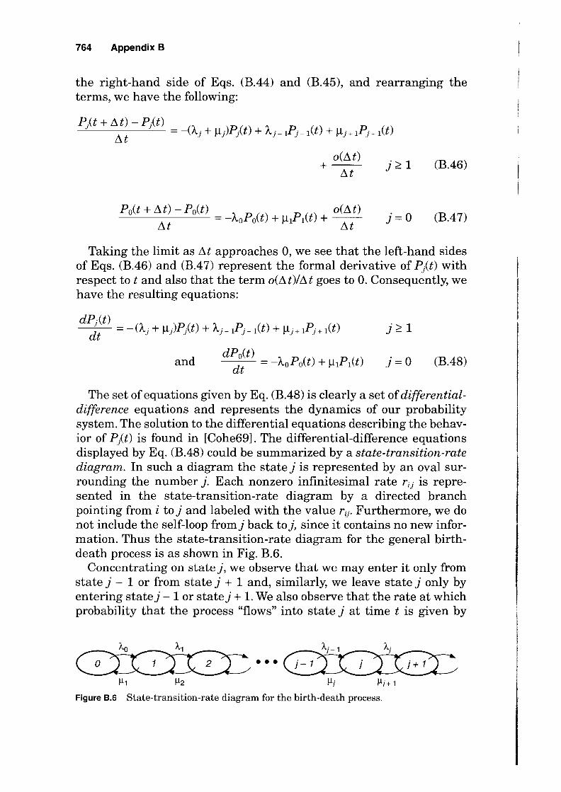
The set of equations given by Eq. (B,48) is clearly a set of differentialdifference equations and represents the dynamics of our probability system. The solution to the differential equations describing the behavior of Pit) is found in [Cohe69]. The differential-difference equations displayed by Eq. (B,48) could be summarized by a state-transition-rate diagram. In such a diagram the state} is represented by an oval surrounding the number }. Each nonzero infinitesimal rate rij is represented in the state-transition-rate diagram by a directed branch pointing from i to} and labeled with the value ri). Furthermore, we do not include the self-loop from} back to}, since it contains no new information. Thus the state-transition-rate diagram for the general birthdeath process is as shown in Fig. B.6.

Concentrating on state}, we observe that we may enter it only from state} - 1 or from state} + 1 and, similarly, we leave state} only by entering state} - 1 or state} + 1. We also observe that the rate at which probability that the process "flows" into state} at time t is given by

••• !Il !I2 !Ii !Ii + 1

Figure B.6 State-transition-rate diagram for the birth-death process.


Aj -lPj-l(t) + Il j + lPj+ let), whereas the flow rate out of the statej at time t is given by (Aj + Ilj)Pit).

8.3.5 Poisson processes

The simplest birth-death process to consider is a pure birth system in which Ilj = 0 Vj and Aj = A Vj. Substituting this into our Eq. (BA8), we have

dP/t) ~P () ~P () . > 1 dt = -I\, j t + I\, j - 1 t J -

dPo(t) = -APo(t) dt

j=O (BA9)

For simplicity we assume that the system begins at time 0 with 0 members, that is,

PiO) = { ~ Solving for poet) we have immediately

poet) = e-At

Inserting this last into Eq. (BA9) for j = 1 results in

dPl(t) _ ~P () ~-At dt - -I\, 1 t + I\,e

The solution to this differential equation is clearly

(B.50)

Continuing by induction, then, we finally have as a solution to Eq. (BA9)

P .( ) = (At)} -At J t ., e

J. j'C. 0, t 'C. 0 (B.51)

This is the celebrated Poisson distribution. It is a pure birth process with constant birth rate A giving rise to a sequence of birth epochs that constitute a Poisson process.

With the initial condition in Eq. (B.50), P;Ct) gives the probability thatj arrivals occur during the time interval (O,t). It is intuitively clear, since the average arrival rate is A, that the average number of arrivals in an interval of length t must be At. In fact both the mean and the variance of a Poisson process are equal to At.

766 Appendix B

8.4 Statistical Techniques

B.4.1 Parameter estimation

Among the most important characteristics of a random variable are its probability distribution, mean, and variance. In practice, means and variances are usually unknown parameters. This subsection discusses how to estimate these parameters from data [Hogg83, Mood74].

B.4.1.1 Point estimation. Point estimation is often used in reliability analysis. Examples include the estimation of the detection coverage from fault injections and the estimation of mean time to failures (MTTF) from field data. Each fault injection and each failure occurrence can be treated as a sample, which is assumed to be independent of other samples.

Given ~ collection of n sampling outcomes, Xl, X2, ••. , X n , of a random variable X, each Xi can be considered as a realization of the random variable Xi. These X;'s are independent of each other and identically distributed as X The set {XI, X 2, ••• , Xnl is called a random sample of X Our purpose is to estimate the value of some parameter 8 (8 could be E[X] or Var(X)) of X using a function of Xl, X 2 , ••• , X n. The function used to estimate 8,8 = 8(Xh X2, ... ,Xn)' is called an estimator of8, and 8(Xl,X2, ... ,xn) is said to be a point estimate of8.

An estimator 8 is called an unbiased estimator of 8, if E[e] = 8. The unbiased estimator that has the minimum variance, i.e., that minimizes Yare e) = E[( 8 - 8)2] among all unbiased estimators frs, is said to be the unbiased minimum-variance estimator. It can be shown that the sample mean

_ 1 n

X=- IXi n i= 1

(B. 52)

is the unbiased minimum-variance linear estimator of the population mean Il, and the sample variance

n

8 2 = 1 I (Xi - X)2 n-l i =l

(B.53)

is, under some mild conditions, an unbiased mInImum-variance guadratic estimator ofthe population variance Var(X). If an estimator 8 converges in probability to 8, that is,

(B.54)

where £ is any small positive number, it is said to be consistent.

Method of maximum likelihood. If the functional form of the pdf of the variable is known, the method of maximum likelihood is a good


approach to parameter estimation. In many cases, approximate functional forms of empirical distributions can be obtained. In such cases, the maximum likelihood method can be used to determine distribution parameters.

The maximum likelihood method is to choose an estimator such that the observed sample is the most likely to occur among all possible samples. The method usually produces estimators that have minimumvariance and consistency properties. But if the sample size is small, the estimator may be biased.

Assuming X has a pdf {(x I e), where e is an unknown parameter, the joint pdf of the sample {Xl. X 2, ••• ,Xn },

L(e) = I17 = 1 {(Xi I e) (B.55)

is called the likelihood (unction ofe. If 8(Xh X2, ... ,xn ) is the point estimate ofe that maximizes L(e), then 8 (Xl, X 2 , ••• ,Xn ) is said to be the maximum likelihood estimator of e. The following example illustrates the method.

Example B.8 Let X denote the random variable time between failures in a computer :;ystem. Assuming X is exponentially distributed with an arrival rate A, we wish to estimate A from a random sample [Xl, X 2, ••• , Xn}. By Eq. (B.55),

How do we choose an estimator such that the estimated A maximizes L(A)? An easier way is to find the A value that maximizes InL(A) instead of L(A). This is because the A that maximizes L(A) also maximizes InL(A), and InL(A) is easier to handle. In this case we have

n

InL(A) = n In(A) - A I Xi

i=l

To find the maximum, consider the first derivative

dllnL(A)] _!!... _ ~ . dA - A LX,

l = 1

The solution of this equation at zero,

is the maximum likelihood estimator for A.

Method of moments. Sometimes it is difficult to find maximum likelihood estimators in closed form. One example is the pdf of the gamma distribution G(a.,e)

768 Appendix B

The estimation of a and e is complicated by the existence of the gamma function rca). The gamma distribution, however, is useful for characterizing arrival times in the real world. In such cases, the method of moments can be used if an analytical relationship is found between the moments of the variable and the parameters to be estimated.

To explain the method of moments, we introduce the simple concepts of sample moment and population moment. The kth (k = 1,2, ... ) sample moment of the random variable X is defined as

1 n k

mk = - I Xi (B.56) n i= 1

where Xl, X 2 , ••• ,Xn are a sample of X The kth population moment of X is just E[Xkj.

Suppose there are k parameters to be estimated. The method of moments sets the first k sample moments equal to the first k population moments, which are expressed as the unknown parameters, and then solves these k equations for the unknown parameters. The method usually gives simple and consistent estimators. However, some estimators may not have unbiased and minimum-variance properties. The following example shows details ofthe method.

Example B.9 We wish to estimate a and A. based on a sample {Xl,X2, •.. ,Xnl from a gamma distribution. Since X - G(a,A.), we know

a a a 2

E[x] = ~ E[x2] = 1..2 + """"i1

The first two sample moments, by definition, are given by 1 n _

ml= - I Xi= X n i= 1

Setting ml =E(X) and m2 =E(X2) and solving for a and A., we obtain -

A X 1..-8 2

These are the estimators for a and A. from the method of moments.

Least-squares estimates. The least-squares estimation technique is commonly applied in engineering and mathematics problems. We assume that a linear law relates two variables, the independent variable x and the dependent variable y:

Y =ax +b

The true data relating y and x are a set of n pairs of points: (Xl, Yl),

(X2, Y2), ... , (xn, Yn). The error between the true value of the dependent variable and the best fit of a linear function is


The error measure for the accuracy of fit is given by the sum of the squared errors (SSE):

n n

SSE = L (errorY = L (Yi - aXi - b)2 i ~ 1 i ~ 1

The best estimates of a and b are the values of a and b that minimize the sum of the squared errors, which is achieved by

GlSSE/Gla = 0 GlSSE/Glb = 0

Solving for the resulting values of a and b yields

and

where

a== L7~1 (Yi - Y)(Xi - x)

L7~1 (Xi - X)2

1 n

x= - L Xi n i= 1

1 n

Y= - LYi n i = 1

(B.57)

(B.58)

The symbols a and 6 stand for the least-squares estimates of a and b, respectively. Note that we can also perform least-squares estimation in a similar manner with other nonlinear functional relationships between Y and x.

B.4.1.2 Interval estimation. So far, our discussion has been limited to the point estimation of unknown parameters. The estimate may deviate from the actual parameter value. To obtain an estimate with a high confidence, it is necessary to construct an interval estimate such that the interval includes th~ actual parameter value with a high probability. Given an estimator e, if

(B.59)

the random interval (8 - el, 8 + e2) is said to be 100 x p percent confidence interval for e, and P is called the confidence coefficient (the probability that the confidence interval contains e).

Confidence intervals for means. In the following discussion, the sample mean X is used as the estimator for the population mean. As mentioned in Sec. B.4.l.1, it is the unbiased minimum variance linear estimator for /-l. Let's first consider the case in which the sample size is

770 Appendix B

large. By the central limit theorem, X is asymptotically normally distributed, no matter what the population distribution is. Thus, when the sample size n is reasonably large (usually 30 or above, sometimes 50 or more if the population distribution is badly skewed with occasional outliers), Z = (X - ~)/(S/Vn) can be approximately treated as a standard normal variable. To obtain a 100 ~ percent confidence interval for~, we can find a number Za/2 from the normal distribution N(O, 1) table such that P(Z > Za/2) = a/2, where a = 1 - ~. Then we have

X-~ P(-Za/2< Vn <za/2)=1-a

S/ n

Thus, the 100(1- a) percent confidence interval for ~ is approximately

- S - S X - Za/2 Vn < ~ < X + Za/2 Vn (B.60)

If the sample size is small (considerably smaller than 30), the above approximation can be poor. In this case, we consider two commonly used distributions: normal and exponential. If the population distribution is normal, the random variable T = (X - ~)I(S/Vn) has a Student's t-distribution with n - 1 degrees of freedom. By repeating the same approach performed above with a t-distribution table, the following 100(1- a) percent confidence interval for ~ can be obtained:

- S S X - tn - 1'a/2 ,I < ~ < X + tn -1'a/2 ,I , vn ' vn

(B.61)

where tn -1;a/2 is a number such that peT > tn -1;a/2) = a/2. Theoretically, Eq. (B.61) requires X to have a normal distribution. However, this estimator is not very sensitive to the distribution of X when the sample size is reasonably large.

If the population distribution is exponential, it can be shown that X2 = 2nX/~ has a chi-square distribution with 2n degrees of freedom. Thus, we can use the chi-square distribution table. Because the chisquare distribution is not symmetrical about the origin, we need to find two numbers, x22n;1_ a/2 and X22n;al2, such that P(X

2 < x22n;1_ a/2) =

a/2 and P(X2 > x22n;a/2) = a/2. The obtained 100(1 - a) percent confi

dence interval for ~ is

2nX 2nX ---<~< ----

2 2 X 2n;a/2 X 2n;1- a/2

(B.62)

Confidence intervals for variances. Our discussion focuses on the two commonly used distributions: normal and exponential. If X is normally dis-


tributed, the sample variance 8 2 can be used to construct the confidence interval. It is known that the random variable (n - 1)82/a 2 has a chi-square distribution with n - 1 degrees of freedom. To determine a 100(1- a) percent confidence interval for a 2

, we follow the procedure for constructing Eq. (B.62) to find the numbers X2 n -1;1- a/2 and X2 n -1;a/2 from the chi-square distribution table. The confidence interval is then given by

(n - 1)82 2 (n - 1)82

2 <a < 2 X n - 1;a/2 X n - 1;1 - a/2

(B.63)

Our experience shows that this equation, like Eq. (B.61), is not restricted to the normal distribution when the sample size is reasonably large (15 or more).

If X is exponentially distributed, we can use Eq. (B.62) to estimate the confidence interval for Var(X), because of the exponential random variable, Var(X) equals 1-L2. Since all terms in Eq. (B.62) are positive, we can square them. The result gives a 100(1 - a) percent confidence interval for Var(X):

( 2nX )2 < Var(X) < ( 2nX )2

X2~n;(<1~ X22n;1_a/2

(B.64)

Confidence intervals for proportions. Often, we need to estimate the confidence interval for a proportion or percentage whose underlying distribution is unknown. For example, we may want to estimate the confidence interval for the detection coverage after fault injection experiments. In general, given n Bernoulli trials with the probability of success on each trial being p and the number of successes being Y, how do we find a confidence interval for p? If n is large (particularly when np ~ 5 and n(l - p) ~ 5 [Hogg83]), Yin has an approximately normal distribution, N(I-L,a 2

), with I-L = p and a 2 = p(l - p)ln. Note that Yin is the sample mean, which is an estimator of I-L or p. By Eq. (B.60), the 100(1- a) percent confidence interval for pis

y - ± Za/2 Vp(1- p)ln n

(B.65)

Example B.10 We would like to determine the number of injections required to achieve a given confidence interval for an estimated fault detection coverage. Let n represent the number offault injections and Y the number offaults detected in the n injections. Assume that all faults have the same detection coverage, which is approximately p. Now we wish to estimate p with the 100(1 - a) percent confidence interval being e. By Eq. (B.65), we have

e =Za/2 Yp(l- p)/n (B.66)

772 Appendix B

Solving the equation for n gives us

(B.67)

where n is the number of injections required to achieve the desired confidence interval in estimating p.

For example, assume detection coverage p = 0.6, confidence interval e = 0.05, and confidence coefficient 1- a = 90 percent. Then the required number of injections is

1.645 2 x 0.6 x 0.4 n = 0.05 2 = 260

8.4.2 Distribution characterization

While mean and variance are important parameters that summarize data by single numbers, probability distribution provides further information about the data. Analysis of distributions can help us understand the data in detail and arrive at conclusions regarding the underlying models. For example, if the time to failure and the recovery time for a system are all exponential, then the model is a Markov model; otherwise, it could be one of the other types of models.

8.4.2.1 Empirical distribution. Given a sample of X, the simplest way to obtain an empirical distribution of X is to plot a histogram of the observations, shown in Fig. B.7. The range ofthe sample space is divided into a number of subranges called buckets. The lengths of the buckets are usually the same, although this is not essential. Assume that we have k

y

y6

y3

y4 y2 y1

y5

-------------- -

1---

--- f-------I-

- - f---- --•••

1 2 3 4 5 6

Figure B.7 Histogram for the pdf of X.

,-

f--

k-2 k-1 k


buckets, separated by Xo, XI, ... , Xk, for the given sample of size n. In each bucket, there areYi instances. Clearly, the sample size n is 1:;=lYi. Then, y;ln is an estimation of the probability that X takes a value in bucket i. The histogram is an empirical pdf of X. An empirical cdf can be constructed from the histogram (shown in Fig. B.8):

0 X < Xo

i

Fk(x) = I Yl Xi-I::;; X < Xi (B.68) 1=1 n

1 Xk::;; X

The key issue in plotting histograms is to determine the bucket size. A small size may lead to such a large variation among buckets that the distribution cannot easily be characterized. On the other hand, a large size may lose details of the distribution. Given a data set, it is possible to obtain very different distribution shapes by using different bucket sizes. One guideline is that if any bucket has less than five instances, the bucket size should be increased or a variable bucket size should be used. Normally 10 or more buckets are sufficient in most cases, depending on the sample size.

B.4.2.2 Distribution function fitting. Analytical distribution functions are useful in analytical modeling and simulations. Thus, it is often desirable to fit an analytical function to a given empirical distribution. Function fitting relies on knowledge of statistical distribution functions. Given an empirical distribution, step 1 is to make a good guess of the closest distribution function(s) based on the shape of the empirical

Fk(x) 1.0 -- --- --------- --- -- --- ------------,-

(y1 + y2 + y3)/n ----,-----i

(y1 + y2)/ n --,y1/n-

-

Figure B.B Histogram for the cdf of X.

-

-

•••

774 Appendix B

distribution, prior knowledge, and intuition. Step 2 is to use a statistical package to obtain the parameters for a guessed function by trying to fit it to the empirical distribution. Step 3 is to test the goodness-offit to see ift~e fitted function is acceptable. If the function is not acceptable, we go to step 1 to try a different function.

Let's loo~ at step 3-the significance test. Assume that the given empirical cdf is Fh , defined in Eq. (B.68), and the hypothesized cdf is F(x), obtained from step 2. Our task is to test the hypothesis

Ro : Fk(x) = F(x)

Two commonly used goodness-of-fit test methods are the chi-square test and the Kolmogorov-Smirnov test. We now briefly introduce these tW9 methods [Dani90].

8.4.2.3 Chi-square test. The chi-square test assumes the distribution under consideration can be approximated by a multinomial distribution. Assume X comes from the distribution F(x). Let

i = 1, ... ,k

where Pi is the probability that an instance falls into bucket i (that is, the interval [Xi _ l> xJ). For a random sample of size n, Xl> X 2 , ••• ,Xn , we form a new random variable to count the number of instances in each bucket:

where

n

Yi = I I[x;_l~Xj~x;l )=1

i = 1, ... , k

Xi_1-:o,X-:o, X i

otherwise

(B.69)

Yi has ajoint multinomial distribution, where the expected instances falling into bucket i is npi. Furthermore, the sum of error squares divided by the expected numbers

k (Yi - np;)2 qh-1=I (B.70)

i= 1 npi

is a measure of the closeness of the observed number of instances, Yi, to the expected number of instances, npi, in bucket i. If qk -1 is small, we tend to accept Ro. This can be measured in terms of statistical significance if we treat qk-1 as a particular value of the random variable Qk-1. It can be shown that if n is large (npi ~ 1), the distribution of Qk -1 is approximately a chi-square distribution with k - 1 degrees of freedom,


X2(k - 1). If Ho is true, we expect qk -1 to fall into an acceptable range of Qk - h so that the event is likely to occur. The boundary value, or critical value, ofthe acceptable range, X~(k - 1) is chosen such that

P[Qk-1 > X;(k -1)] = ex

where ex is called the significance level of the test. Thus, we should reject Ho if qk -1> X;(k - 1). Usually, ex is chosen to be 0.05 or 0.1.

Example B.11 Mendelian theory indicates that the shape and color of a certain variety of pea ought to be grouped into four groups, "round and yellow," "round and green," "angular and yellow," and "angular and green," according to the ratios 9/3/3/1. For n = 1600 peas, the following were observed (the last column gives the expected number):

Round and yellow Round and green Angular and yellow Angular and green

948 279 284

89

900 300 300 100

A 0.05 significance level test of the null hypothesis Ho: PI = 9/16, P2 = 3/16, P3 = 3/16, andp4 = 1116 is given by the following: reject Ho if and only if q3 = Li (y;

2 2 - npY/npi exceeds X I_a(k) = X.95 (3) = 7.81. The observed q3 is

(948 - 900)2 (279 - 300)2 (284 - 300? (89 - 100)2 900 + 300 + 300 + 100 = 6.09

and so there is good agreement with the null hypothesis; that is, there is a good fit between the data and the model.

8.4.2.4 Kolmogorov-Smirnov test. The Kolmogorov-Smirnov test is another nonparametric method in that it assumes no particular distribution for the variable in consideration. The method uses the empirical cdf, instead of the empirical pdf, to perform the test, which is more stringent than the chi-square test. It can be shown that Fk(x) in Eq. (B.68) has an asymptotic normal distribution. Namely, Vk [Fk(x) - F(x)] has a limiting normal distribution with mean 0 and variance F(x)[1 - F(x)]. The Kolmogorov-Smirnov statistic is thus defined by

(B. 71)

where supx represents the least upper bound of all pointwise differences I Fk(x) -F(x) I. In calculation, we can choose the midpoint between Xi-1

and Xi, for i = 1, ... , k, to obtain the maximum value of I Fk(x) - F(x) I. It is seen that Dk is a measure ofthe closeness ofthe empirical and hypothesized distribution functions. It can be derived that Dk follows a distribution whose cdf values are given by the table of Kolmogorov-Smirnov

776 Appendix B

acceptance limits [Hand66]. Thus, given a significance level a, we can find the critical value dk from the table such that

The hypothesis Ro is rejected if the calculated value of Dk is greater than the critical value d k • Otherwise, we accept Ro.

Example B.12 A hospital is interested in knowing whether the times of birth are uniformly distributed over the hours of the day. For 37 consecutive births in the hospital, the following times were observed: 1:53 P.M., 3:06 P.M., 6:45 P.M., 6:26 A.M.,

$:12 A.M., 10:45 A.M., 2:02 P.M., 11:46 P.M., 12:26 A.M., 5:49 A.M., 8:40 A.M., 2:17 P.M.,

4:09 P.M., 4:44 P.M., 7:02 P.M., 11:08 P.M., 11:45 P.M., 3:56 A.M., 5:08 A.M., 9:06 A.M.,

11:19 A.M., 12:25 P.M., 1:30 P.M., 3:57 P.M., 2:28 A.M., 6:32 A.M., 7:40 A.M., 8:25 A.M.,

12:40 P.M., 12:55 P.M., 3:22 P.M., 4:31 P.M., 7:46 P.M., 1:24 A.M., 3:02 A.M., 10:06 A.M.,

10:07 A.M. Both the hypothesized uniform cdf and the sample cdf are sketched in Fig. E.9.

One can calculate supx I Fk(x) - F(x) I = I (31137) - (1004/1440) I = 0.1406.

The critical value for significance a = 0.10 is greater than 0.2; so, according to the Kolmogorov-Smirnov goodness-of-fit test, the data do not indicate that the hypothesis that times of birth are uniformly distributed throughout the hours of the day should be rejected. (That is, there is a good fit of the data.)

B.4.3 Multivariate analysis

In reality, measurements usually consist of realizations from multiple variables. For example, a computer workload measurement may in-

y

o 4 A.M.

240

I I I I I I I I I I I I

:/4:44 P.M.

8 A.M. 12 noon 4 P.M. 8 P.M. 1440 x 480 720 960 1200 min.

Figure B.9 Uniform cdf and sample cdf ofthe birth data.


clude usages on the CPU, memory, disk, and network. A computer failure measurement may collect data on multiple components. Multivariate analysis is the application of methods that deal with multiple variables [Dill84, Kend77, John82]. These methods, including cluster analysis, correlation analysis, and factor analysis, identify and quantify relationships among multiple variables.

8.4.3.1 Correlation analysis. The correlation coefficient, Cor(Xt, X 2),

between two random variables Xl and X2 is defined as

(B.72)

where j.ll and j.l2 are the means of Xl and X2 and 0"1 and 0"2 are the standard deviations of Xl andX2, respectively. Ifwe use p to denote the correlation coefficient of Xl and X 2 , then p satisfies -1 ~ P ~ 1. The correlation coefficient is a measure of the linear relationship between two variables. When I p I = 1, we have Xl = aX2 + b, where a > ° if p = 1, and a < ° if p = -1. In these extreme cases, there is an exact linear relationship between Xl andX2. When I p I =1-1, there is no exact linear relationship between Xl and X 2• In this case, p measures the goodness of the linear relationship Xl = aX2 + b between Xl and X 2 •

If a random variable, X, is defined on time series, the correlation coefficient can be used to quantify the time serial dependence in the sample data of X. Given a time window !It > 0, the autocorrelation coefficient of X on the time series t is defined as

Autocor(X, M) = Cor (X(t), X(t + M» (B.73)

where t is defined on the discrete values (M, 2M, 3M, ... ). In this case, we treatX(t) andX(t + !It) as two different random variables, and the autocorrelation coefficient is actually the correlation coefficient between the two variables. That is, Autocor(X,!lt) measures the time serial correlation of X with a window M.

8.4.3.2 Factor analysis. The limitation of correlation analysis is that the correlation coefficient can only quantify a dependency between two variables. However, dependencies may exist within a group of more than two variables or even among all variables. The correlation coefficient cannot provide information about such multiway dependencies. Factor analysis is a statistical technique to quantify multiway dependencies among variables. The method attempts to find a set of unobserved common factors that link together the observed variables. Consequently, it provides insights into the underlying structure of the data. For example, in a distributed system, a disk crash can account for

778 Appendix B

failures on those machines whose operations depend on a set of critical data on the disk. The disk state can be considered to be a common factor for failures on these machines.

Let X = (Xl, ... ,Xp)T be a normalized random vector. We say that the k-factor model holds for X if X can be written in the form

(B.74)

where A = (Ai) (i = 1, ... ,p;j = 1, ... ,k) is a matrix of constants called factor loadings, and F = (fl, . .. ,{kl and E = (eb ... ,epl are random vectors. The elements ofF are called common factors, and the elements of E are called unique factors (error terms). These factors are unobservable variables. It is assumed that all factors (both common factors and unique factors) are independent of each other and that the common factors are normalized.

Each variable Xi (i = 1, ... ,p) can then be expressed as

k

Xi = I AiJj + ei j=l

and its variance can be written as

k

cr~ = I A~j + 'Vi j=l

where 'Vi is the variance of ei. Thus, the variance of Xi can be split into two parts. The first part

k

h = A 2 I 2 , U

j=l

is called the communality. It represents the variance of Xi that is shared with the other variables via the common factors. In particular Ai) = Cor(xi,!) represents the extent to which Xi depends on thejth common factor. The second part, 'Vi, is called the unique variance. It is due to the unique factor ei and explains the variability in Xi not shared with the other variables.

8.4.3.3 Cluster analysis. Cluster analysis is helpful in identifying patterns in data. More specifically, it helps in reading a large number of points plotted in an n-dimensional space into a few identifiable states called clusters. For example, it can be used for characterizing workload states in computer systems by identifying the points in a resource usage plot that are similar by some measure and grouping them into a cluster. Assume we have a sample of p workload variables. We call each instance in the sample a point characterized by p values. Let Xi = (XiI,


Xi2, ..• ,Xip) denote the ith point of the sample. The Euclidean distance between points i andj,

is usually used as a similarity measure between points i andj. There are several different clustering algorithms. The goal of these

algorithms is to achieve small within-cluster variation relative to the between-cluster variation. A commonly used clustering algorithm is the k-means algorithm. The algorithm partitions a sample with p dimensions and n points into k clusters, CI, C2, ••• ,Ck • The mean, or centroid of the C j is denoted by Xj' The error component of the partition is defined as

k

E= I I 1 Xi - Xj 12 (B.75) j= lX i ECj

The goal ofthe k-means algorithm is to find a partition that minimizes E The clustering procedure starts with k groups, each of which consists

of a single point. Each new point is added to the group with the closest centroid. After a point is added to a group, the mean of that group is adjusted to take into account the new point. After a partition is formed, the procedure searches for another partition with smaller Eby moving points from one cluster t~ another cluster until no transfer of a point results in a reduction in E [SpatSO].

The presence of outliers in the sample is a problem associated with the clustering algorithms. Outliers can be an order of magnitude greater than most (usually more than 95 percent) of the other points of the sample and can be scattered over the sample space. As a result, the generated clusters may not characterize the features of the sample well. For example, most generated clusters may contain only one or two outliers, with all other points groupable into only a few clusters. One way to deal with this problem is to specify in the algorithm the minimum number of points to form a cluster, typically 0.5 percent of the sample size. Another way is to define an upper bound for the radius (maximum distance between the centroid and any point in a cluster) of any generated cluster. A recommended range for the upper bound is 1.0 to 1.5 standard deviations of the sample [ArtiS6].

review of reliability theory, analytical techniques, and basic

Documents