review of macroeconomics su, chapter 5. historical background beginning of modern economics: inquiry...
TRANSCRIPT

Review of Macroeconomics
Su, Chapter 5

Historical Background
• Beginning of modern economics: Inquiry into the Nature and Causes of the Wealth of Nations, Adam Smith, 1776
• Before Smith: Malthusian Economies; poverty and shortage; inability to sustain populations.

Classical Theory
• Economic theories developed from the publication of Wealth of Nations to about 1870
• Classical theorists:– Adam Smith (1723-1790)– David Ricardo (1772-1823)– Thomas Malthus (1776-1834)– John Stuart Mill (1806-1873)

Main Points of Classical Theory• Develop laws describing value, production and
distribution• Laissez-Faire Economics: “You think you are
helping the economic system by your well meaning laws and inferences. You are not.”
• Supply Side Emphasis: Focus was production, not income. Specialization and division of labor.– Say’s Law: Supply creates its own demand. Go ahead
and produce, don’t worry about demand, markets take care of that.

Neoclassical Theory
• Shift to analytical methods after 1870– Marginal analysis
• William Jevons (1835-1882), Leon Walras (1834-1910), Karl Menger (1849-1921)
• Emphasis on both supply and demand: demand focus followed marginal analysis
• Quantity theory of moneyMxV=PxQ M: Money Supply, P: Price Level, Q: Output,
V: Velocity of Money (times money stock is spent)

Keynesian Revolution
• Brought about by the Great Depression, which Neoclassical theory could not explain– Households could not purchase what was
produced
• The General Theory of Employment, Interest, and Money, John Maynard Keynes
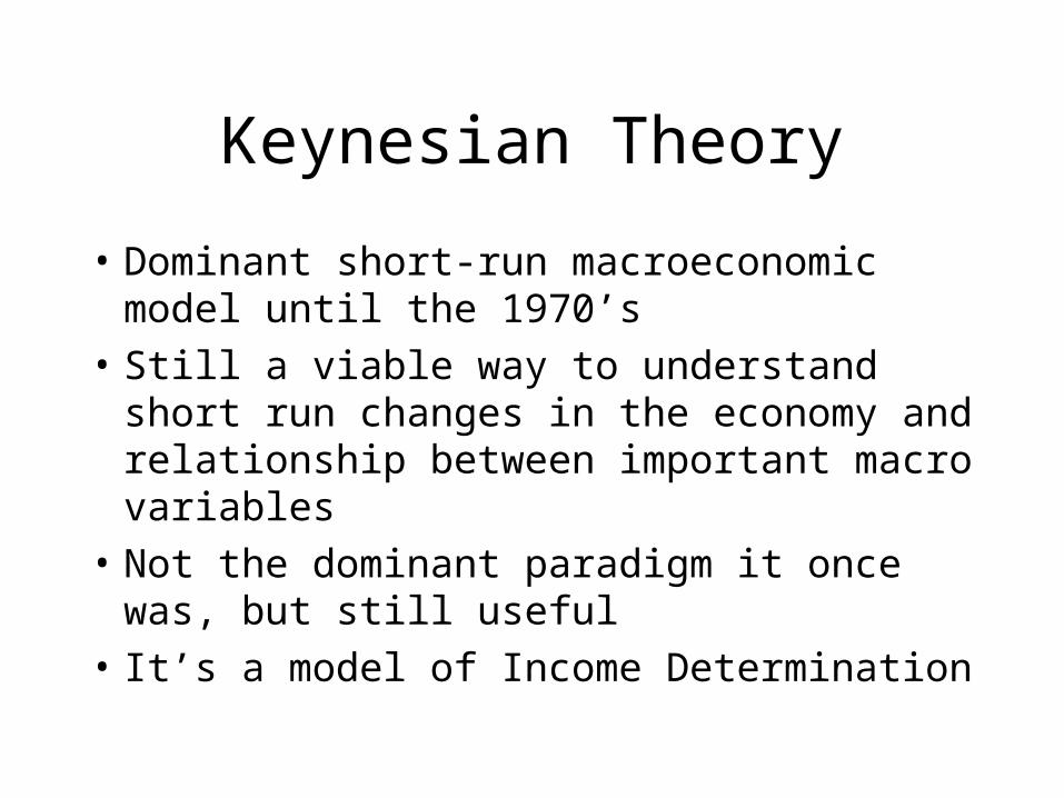
Keynesian Theory
• Dominant short-run macroeconomic model until the 1970’s
• Still a viable way to understand short run changes in the economy and relationship between important macro variables
• Not the dominant paradigm it once was, but still useful
• It’s a model of Income Determination
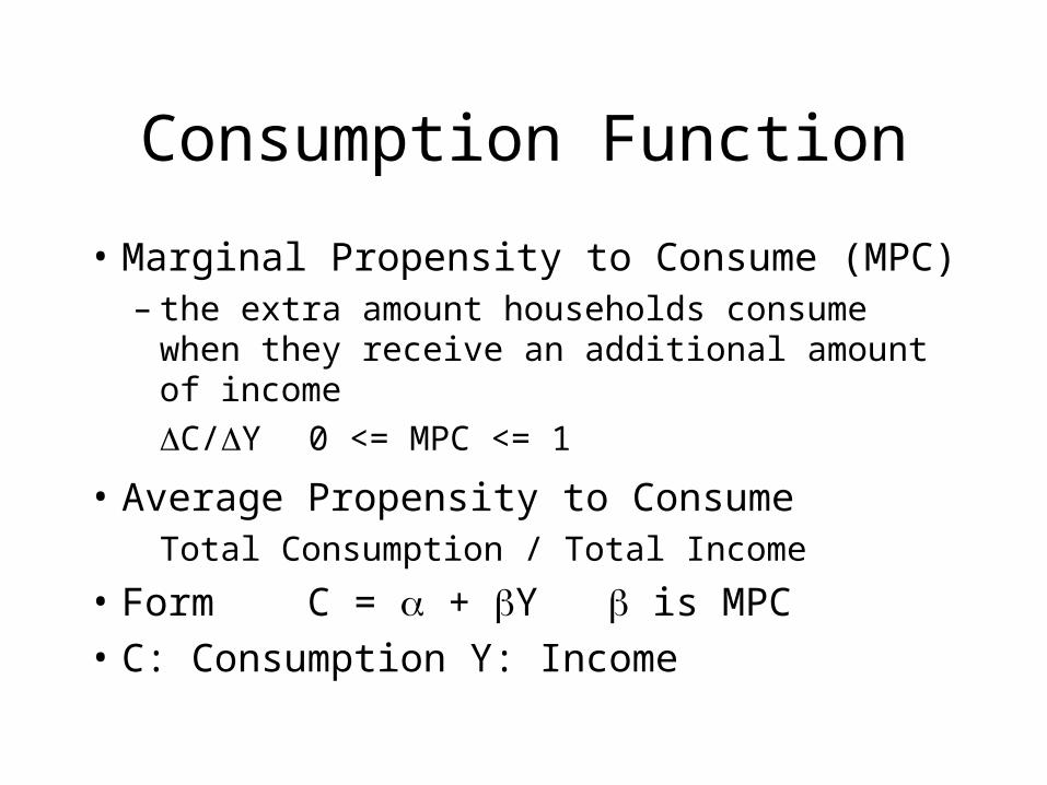
Consumption Function
• Marginal Propensity to Consume (MPC)– the extra amount households consume when
they receive an additional amount of income C/Y 0 <= MPC <= 1
• Average Propensity to Consume Total Consumption / Total Income
• Form C = + Y is MPC
• C: Consumption Y: Income
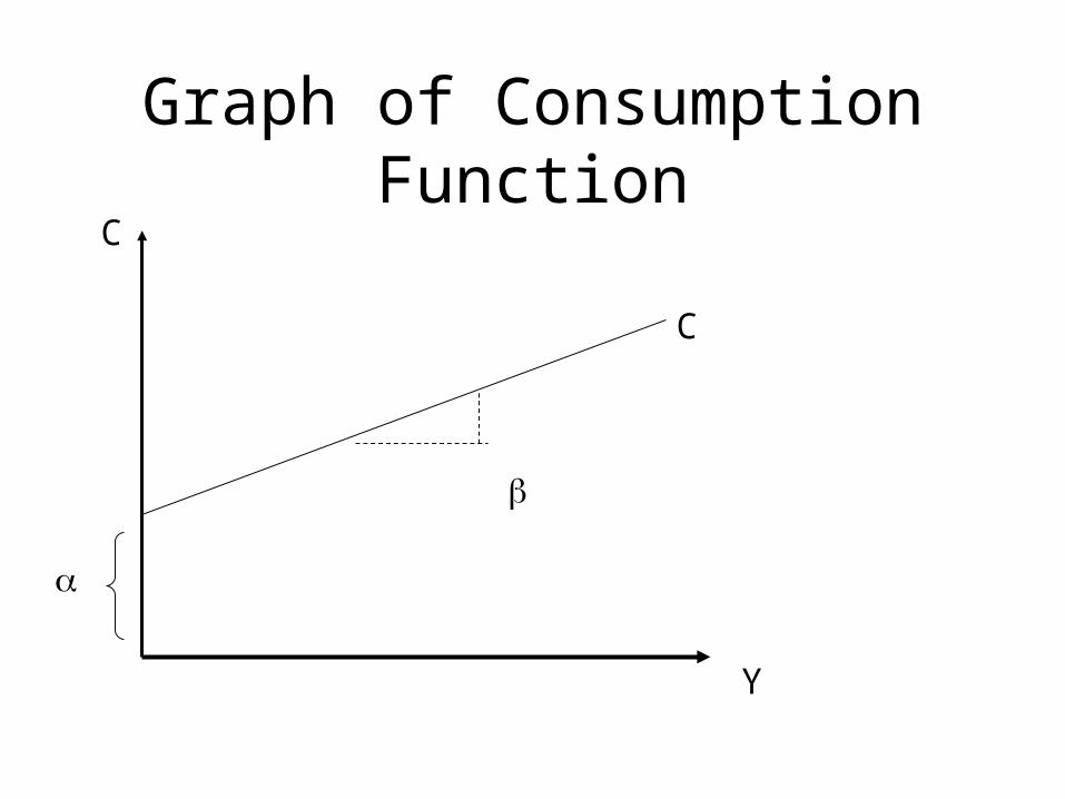
Graph of Consumption Function
Y
C
C

Disposable Income
• For now, suppose that YD = Y = C + S
– Where S: Savings
• Implies I = S, equilibrium condition

Income Identity
• For simplicity, Suppose X=G=M=0
• Then Y (or GDP) = C + I = SP
45o
Y
GDP = SP

Income Identity: A Clarification
• At first, the relationship between the income identity and the 45o line may seem unclear, because there’s an implicit step.
• INCOME (Y) = SPENDING (SP)• SPENDING (SP) = C + I + G + X - M• So the 45o line shows all points where Income
equals spending
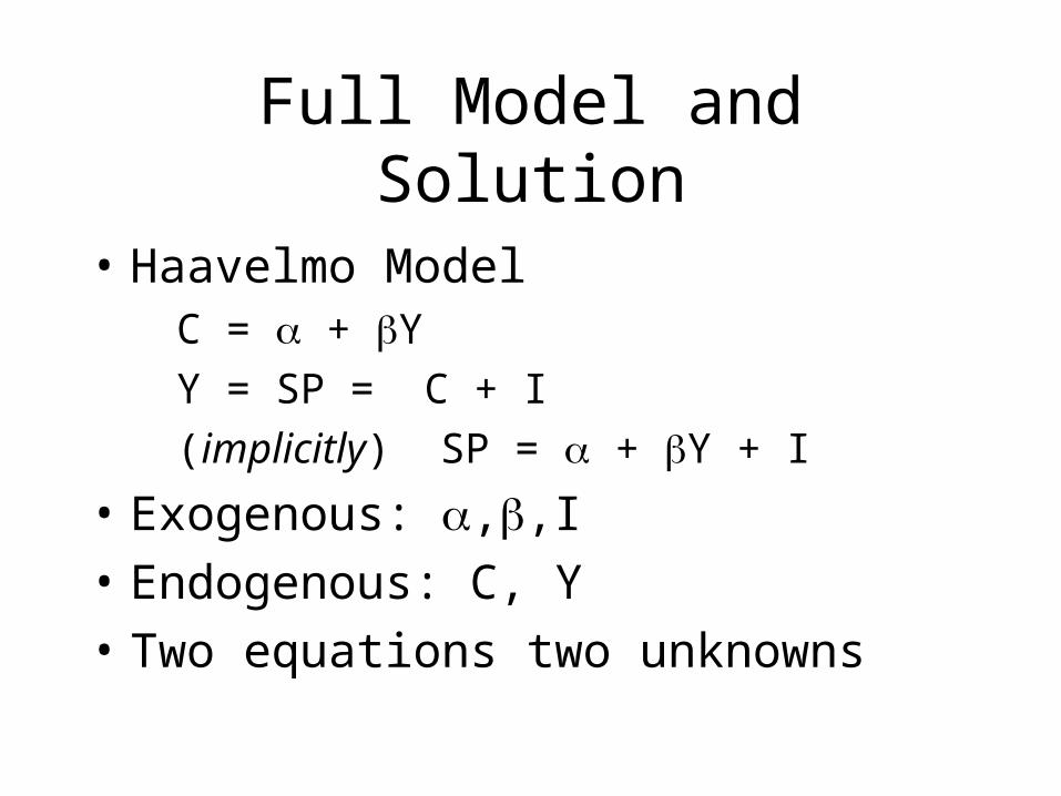
Full Model and Solution
• Haavelmo Model C = + Y Y = SP = C + I (implicitly) SP = + Y + I
• Exogenous: ,,I
• Endogenous: C, Y
• Two equations two unknowns

Algebraic Solution
• C* = [/(1-)] + [/(1-)] I
• Y* = [/(1-)] + [/(1-)] I
• “Reduced Form” Equations: Endogenous Variables on left hand side, Exogenous on right
• Parameters are “Multipliers”/(1-)] > 1

Graphical Solution
Y
SP
+ I
C
Y*
45o

Multiplier Effect
Y
SP
+ I
SP
Y*
45o
SP’
+ I’
Y**

And...
• Note that Investment spending changed by I -I’ = I
• And GDP changed by Y* - Y** = Y
• What can be said about Y relative to I?
• Y* = /(1-)] + [/(1-)] I
• Y** = [/(1-)] + [/(1-)] I’
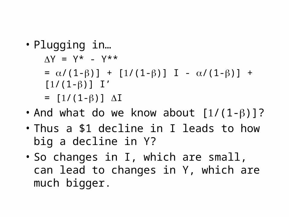
• Plugging in… Y = Y* - Y** = /(1-)] + [/(1-)] I - /(1-)] + [/(1-)] I’ = [/(1-)] I
• And what do we know about [/(1-)]?
• Thus a $1 decline in I leads to how big a decline in Y?
• So changes in I, which are small, can lead to changes in Y, which are much bigger.

Consumption, Investment, Government Spending
0
500
1000
1500
2000
2500
3000
3500
4000
4500
5000
1959 1964 1969 1974 1979 1984 1989 1994
CIG

Extension: Government Spending
• Relax the assumption that G = 0, Now G is an exogenous variable representing government spending C = + Y Y SP = C + I + G (implicitly) SP = + Y + I + G
• Exogenous: ,,I,G• Endogenous: C, Y

Graphical Solution
Y
SP
+I+G
SP
Y*
45o
[/(1-)]

Model with G
• Note that G and I affect the solutions to the model (Y*,C*) in the same way.
• C* = [/(1-)] + [/(1-)] I + [/(1-)] G
• Y* = [/(1-)] + [/(1-)] I + [/(1-)] G
• [/(1-)] is both the Investment Multiplier and the Government Spending multiplier.
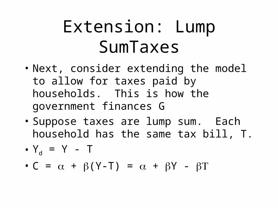
Extension: Lump SumTaxes
• Next, consider extending the model to allow for taxes paid by households. This is how the government finances G
• Suppose taxes are lump sum. Each household has the same tax bill, T.
• Yd = Y - T
• C = + (Y-T) = + Y -

Consumption Function with lump sum T
Y
C
C
- T
CT
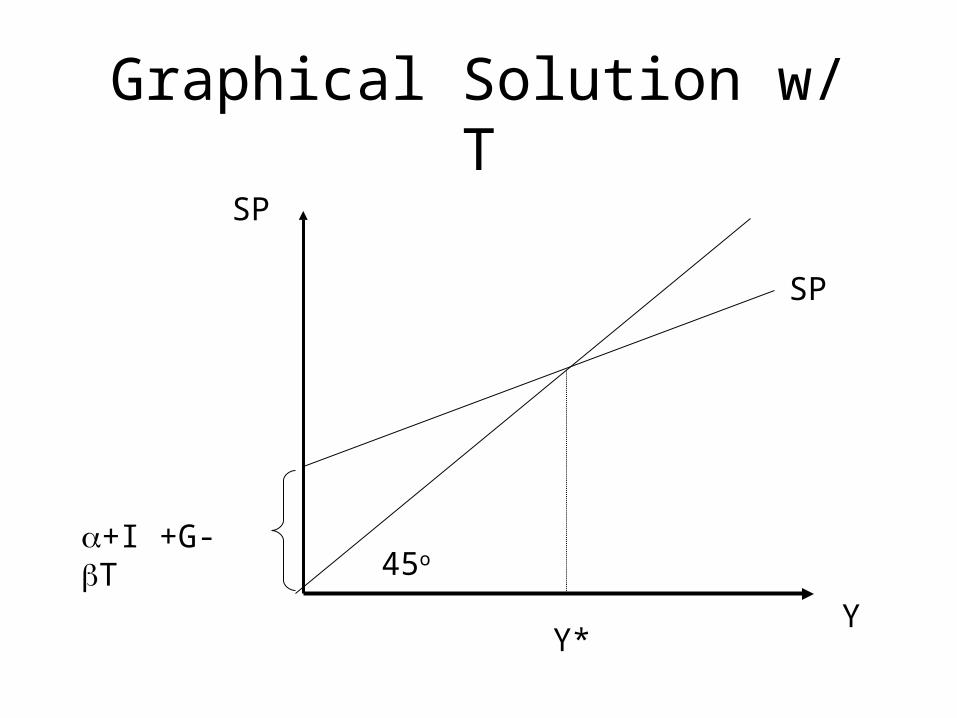
Graphical Solution w/ T
Y
SP
+I +G-T
SP
Y*
45o
Algebraic Solution
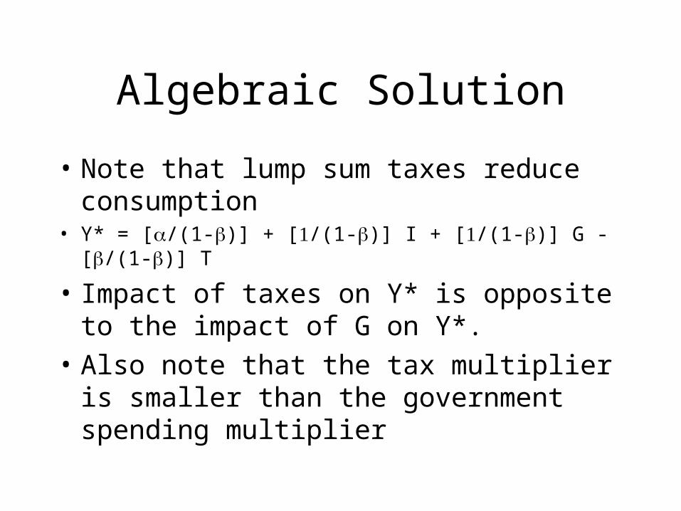
• Note that lump sum taxes reduce consumption
• Y* = [/(1-)] + [/(1-)] I + [/(1-)] G - [/(1-)] T
• Impact of taxes on Y* is opposite to the impact of G on Y*.
• Also note that the tax multiplier is smaller than the government spending multiplier

Model Extension: Proportional Taxation
• Suppose that taxes paid by households are proportional to income
• T = t0 + t1Y (Tax Function)
• Yd = Y - T (Disposable Income)
• C = + Yd
• C = + (Y- t0 - t1Y )
• C = - t0 + - t1)Y
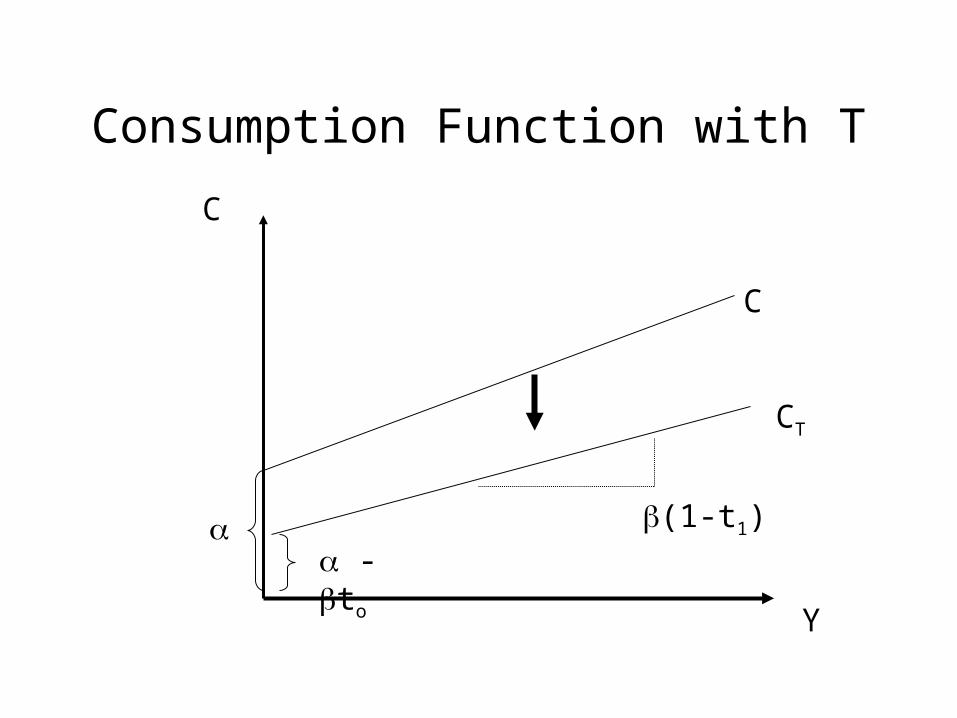
Consumption Function with T
Y
C
C
- to
CT
(1-t1)

Graphical Solution w/ Prop. T
Y
SP
+I +G-t
SP
Y*
45o
(1-t1)
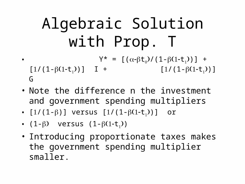
Algebraic Solution with Prop. T
• Y* = [(t/(1-t)] + [/(1-t)] I + [/(1-t)] G
• Note the difference n the investment and government spending multipliers
• [/(1-)] versus [/(1-t)] or
• (1- versus (1-t)
• Introducing proportionate taxes makes the government spending multiplier smaller.

Example I: G = (G2 - G1) > 0
Y
SP
+I +G1-t
SP
Y*
45o
SP’
+I +G2-t
Y**
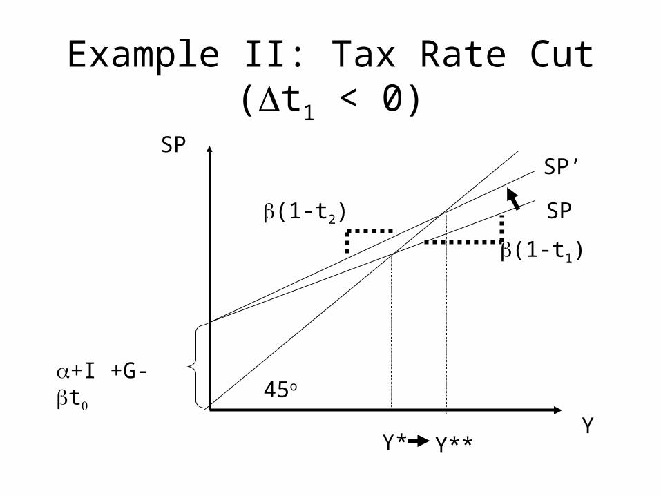
Example II: Tax Rate Cut (t1 < 0)
Y
SP
+I +G-t
SP
Y*
45o
(1-t1)
(1-t2)
SP’
Y**
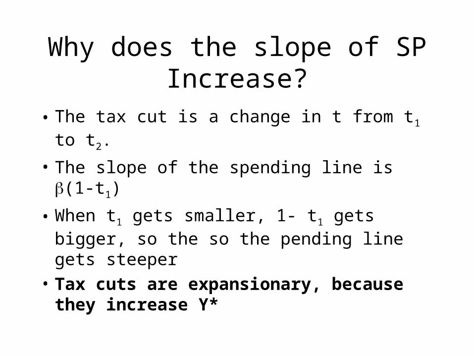
Why does the slope of SP Increase?
• The tax cut is a change in t from t1 to t2.
• The slope of the spending line is (1-t1)
• When t1 gets smaller, 1- t1 gets bigger, so the so the pending line gets steeper
• Tax cuts are expansionary, because they increase Y*
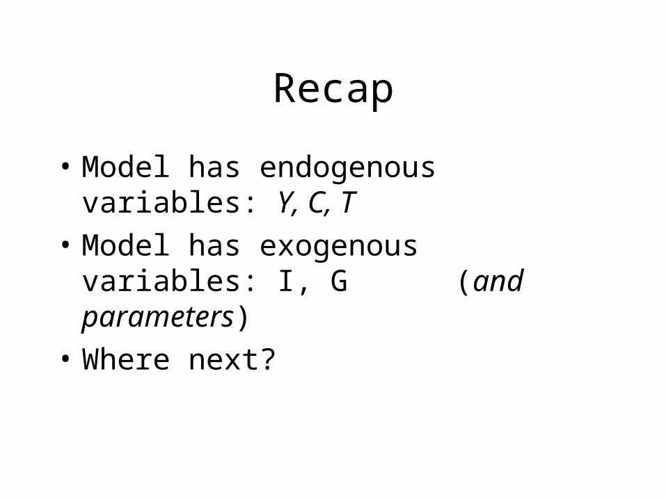
Recap
• Model has endogenous variables: Y, C, T
• Model has exogenous variables: I, G (and parameters)
• Where next?
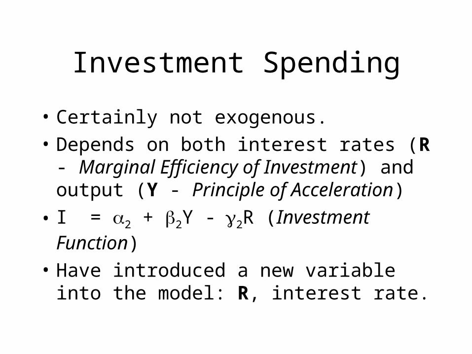
Investment Spending
• Certainly not exogenous.
• Depends on both interest rates (R - Marginal Efficiency of Investment) and output (Y - Principle of Acceleration)
• I = 2 + 2Y -2R (Investment Function)
• Have introduced a new variable into the model: R, interest rate.
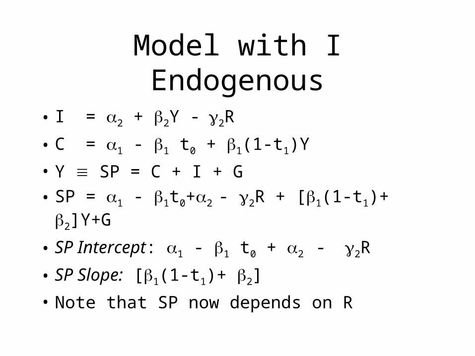
Model with I Endogenous
• I = 2 + 2Y -2R
• C = 1 - 1 t0 + 1(1-t1)Y
• Y SP = C + I + G
• SP = 1 - 1t0+2 - 2R + [1(1-t1)+ 2]Y+G
• SP Intercept: 1 - 1 t0 + 2 - 2R
• SP Slope: [1(1-t1)+ 2]
• Note that SP now depends on R

Y
SP
SP
Y*
45o
SP’
Y**
Effect of R on Y*, R Decreases
1 - 1 t0 + 2 - 2R1
1 - 1 t0 + 2 - 2R2
Y
SP
SP’
Y**
45o
SP
Y*
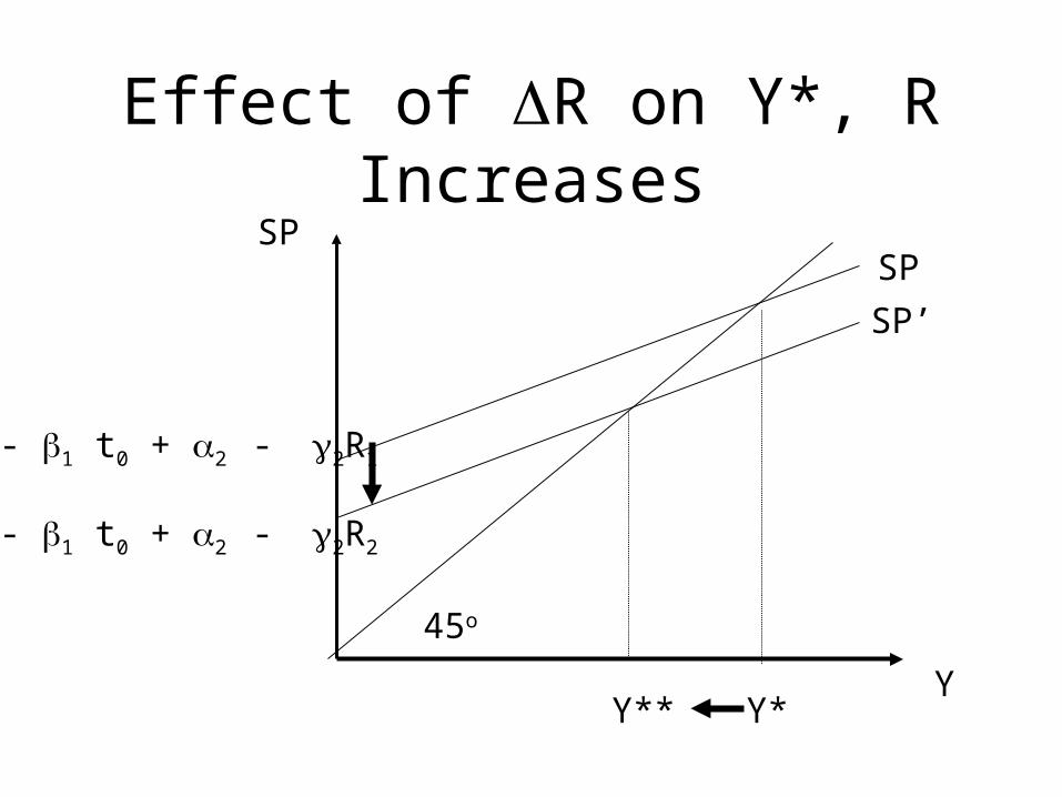
Effect of R on Y*, R Increases
1 - 1 t0 + 2 - 2R1
1 - 1 t0 + 2 - 2R2
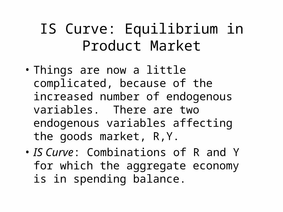
IS Curve: Equilibrium in Product Market
• Things are now a little complicated, because of the increased number of endogenous variables. There are two endogenous variables affecting the goods market, R,Y.
• IS Curve: Combinations of R and Y for which the aggregate economy is in spending balance.

Derivation of IS Curve• Start at A. SP1, and
Y1 depends, in part on R1.
• Map (R1,Y1) into RxY
• Note that A is a combination of R, Y where economy is in spending balance.
• A is on the IS curve
SP
Y
Y
A SP1
R1
Y1
R
AR1

Derivation of IS Curve• Now change R. Let
R decrease to R2. • Find (R2,Y2),new
equilibrium B
SP
Y
Y
A SP1
R1
Y1
R
AR1
SP2
R2
B
Y2
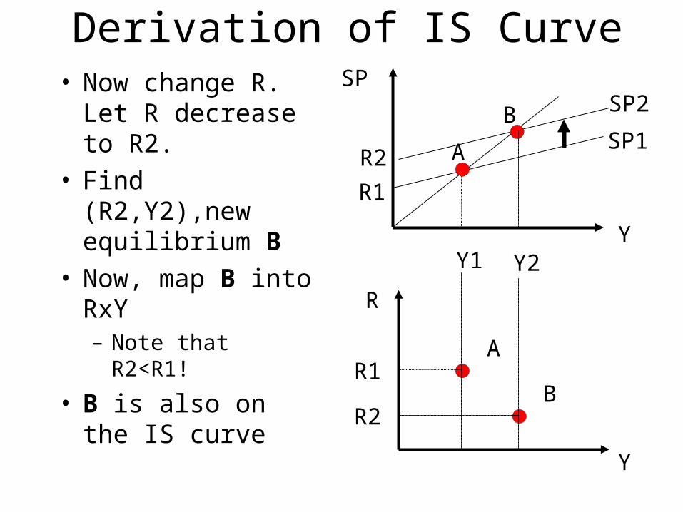
Derivation of IS Curve• Now change R. Let
R decrease to R2. • Find (R2,Y2),new
equilibrium B• Now, map B into
RxY– Note that R2<R1!
• B is also on the IS curve
SP
Y
Y
A SP1
R1
Y1
R
AR1
SP2
R2
B
Y2
R2B
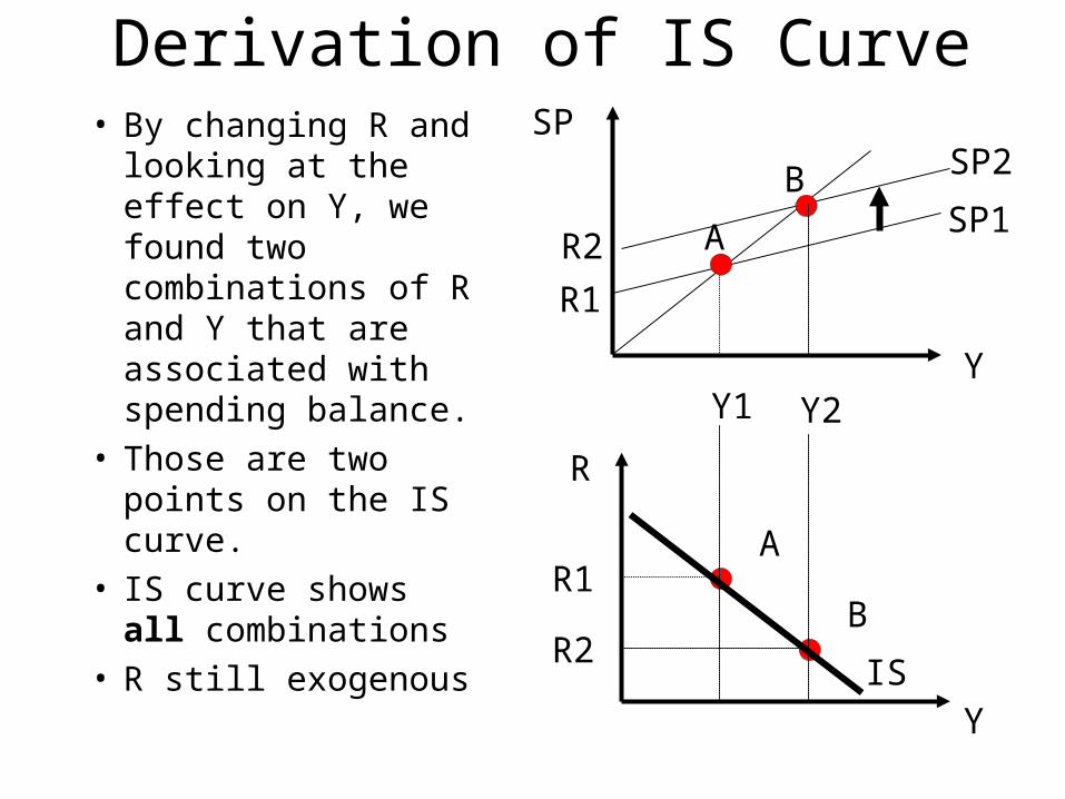
Derivation of IS Curve• By changing R and
looking at the effect on Y, we found two combinations of R and Y that are associated with spending balance.
• Those are two points on the IS curve.
• IS curve shows all combinations
• R still exogenous
SP
Y
Y
A SP1
R1
Y1
R
AR1
SP2
R2
B
Y2
R2B
IS

Algebraic Representation
• To find the equation for the IS curve, solve the following two equation system for R
• Y SP = C + I + G
• SP = 1 - 1t0+2 - 2R + [1(1-t1)+ 2]Y+G
• Giving
• R = (1/2)(1 - 1t0+2+G) - (1/2)(1-1(1-t1)-2)Y
• The first term is the intercept, the second the slope.

Shifts in the IS Curve: G>0• Consider the effects of
an increase in gov. spending on the IS curve.
• Start at A. Note that G is in the intercept of the IS curve.
• When G increases, SP shifts up; move to B
• Where is B in the bottom panel?
• What happened to R?
SP
Y
Y
A SP1
G1
Y1
R
AR1
SP2
G2
B
Y2

Shifts in the IS Curve: G > 0• R was unchanged, so
B must be to the left of A.
• Increases in government spending shift the IS curve to the right.
SP
Y
Y
A SP1
G1
Y1
R
AR1
SP2
G2
B
Y2
B
IS1IS2
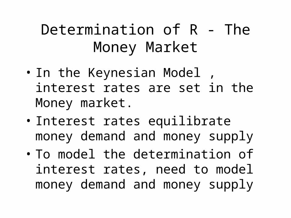
Determination of R - The Money Market
• In the Keynesian Model , interest rates are set in the Money market.
• Interest rates equilibrate money demand and money supply
• To model the determination of interest rates, need to model money demand and money supply
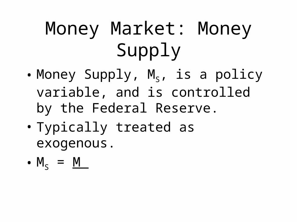
Money Market: Money Supply
• Money Supply, MS, is a policy variable, and is controlled by the Federal Reserve.
• Typically treated as exogenous.
• MS = M

M/P
R
Graphing Money Supply
M/P
MS
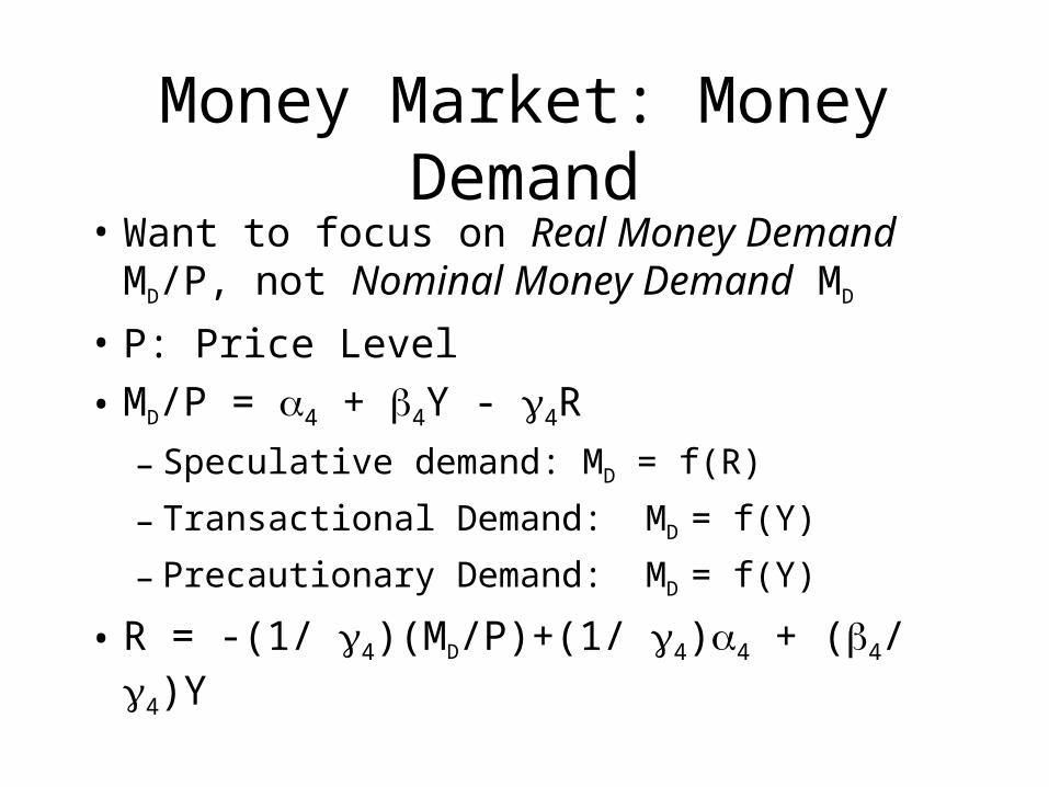
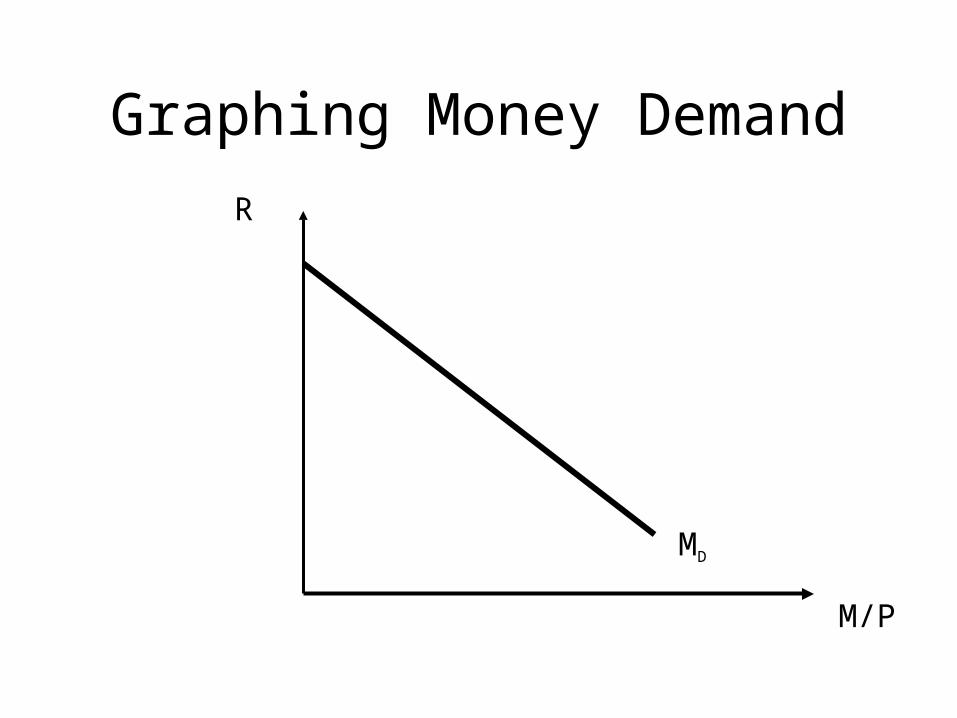
Money Market: Money Demand
• Want to focus on Real Money Demand MD/P, not Nominal Money Demand MD
• P: Price Level
• MD/P = 4 + 4Y - 4R
– Speculative demand: MD = f(R)
– Transactional Demand: MD = f(Y)
– Precautionary Demand: MD = f(Y)
• R = -(1/ 4)(MD/P)+(1/ 4)4 + (4/ 4)Y
M/P
R
Graphing Money Demand
MD

Equilibrium in the Money Market
• The money market is in equilibrium when MS = MD
• Equilibrium is the interest rate R* where money supply equals money demand.

M/P
R
Graphing Money Market Equilibrium
MD
M/P
MS
R*

M/P
R
Shifts in MD: Y > 0
MD
M/P
MS
R*M’D
R**

The LM Curve: Equilibrium in the Money Market
• Like the goods market, things are now a little complicated. There are two endogenous variables affecting the money market, Y and R.
• LM Curve: Combinations of R and Y for which there is equilibrium in the money market
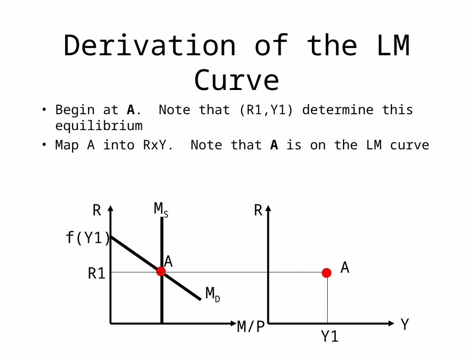
Derivation of the LM Curve
• Begin at A. Note that (R1,Y1) determine this equilibrium
• Map A into RxY. Note that A is on the LM curve
R R
YM/P
MD
MS
f(Y1)
AR1
Y1
A

Derivation of the LM Curve
• Now, suppose Y falls from Y1 to Y2. Find the new equilibrium, B
• Note that R falls to R2.
R R
YM/P
MD
MS
f(Y1)
AR1
Y1
A
M’D
F(Y2)
R2B
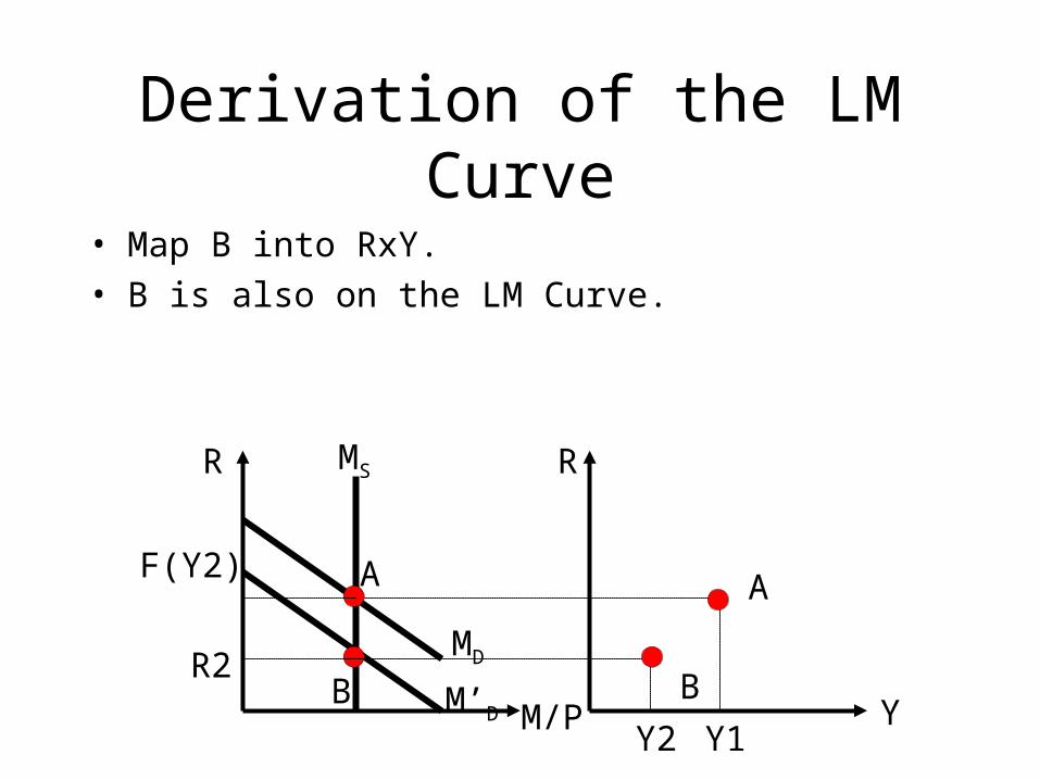
Derivation of the LM Curve
• Map B into RxY.
• B is also on the LM Curve.
R R
YM/P
MD
MS
A
Y1
A
M’D
F(Y2)
R2B
Y2
B
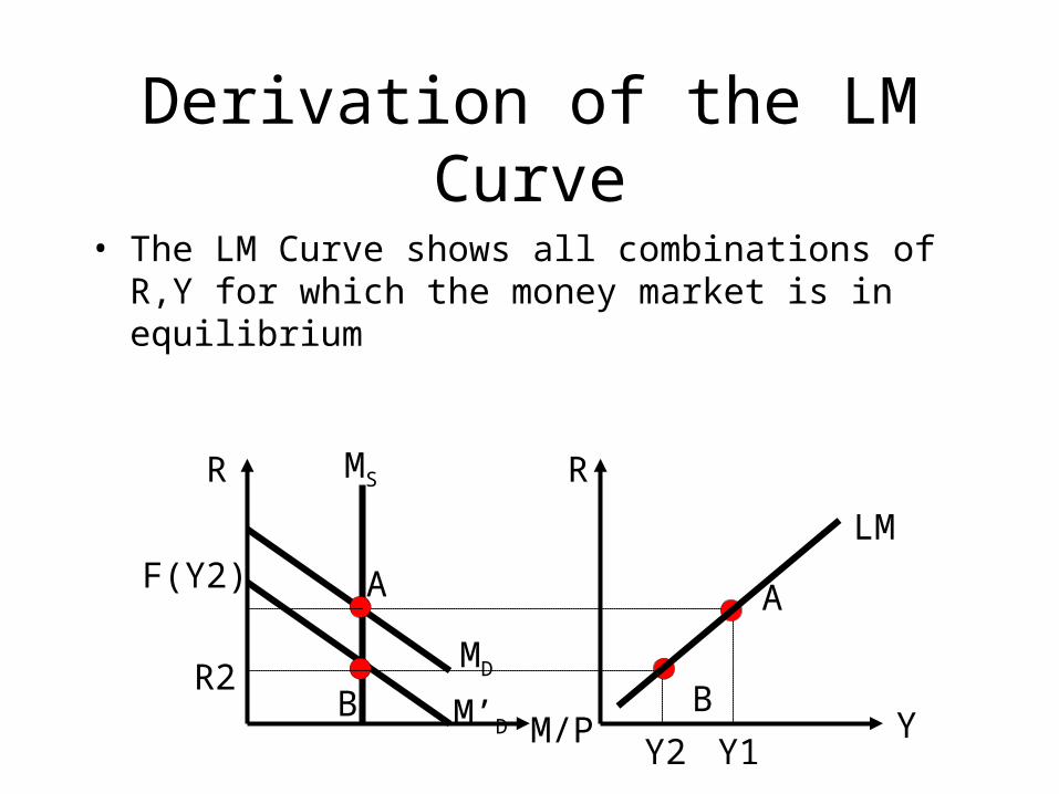
Derivation of the LM Curve
• The LM Curve shows all combinations of R,Y for which the money market is in equilibrium
R R
YM/P
MD
MS
A A
M’D
F(Y2)
R2B B
Y1Y2
LM
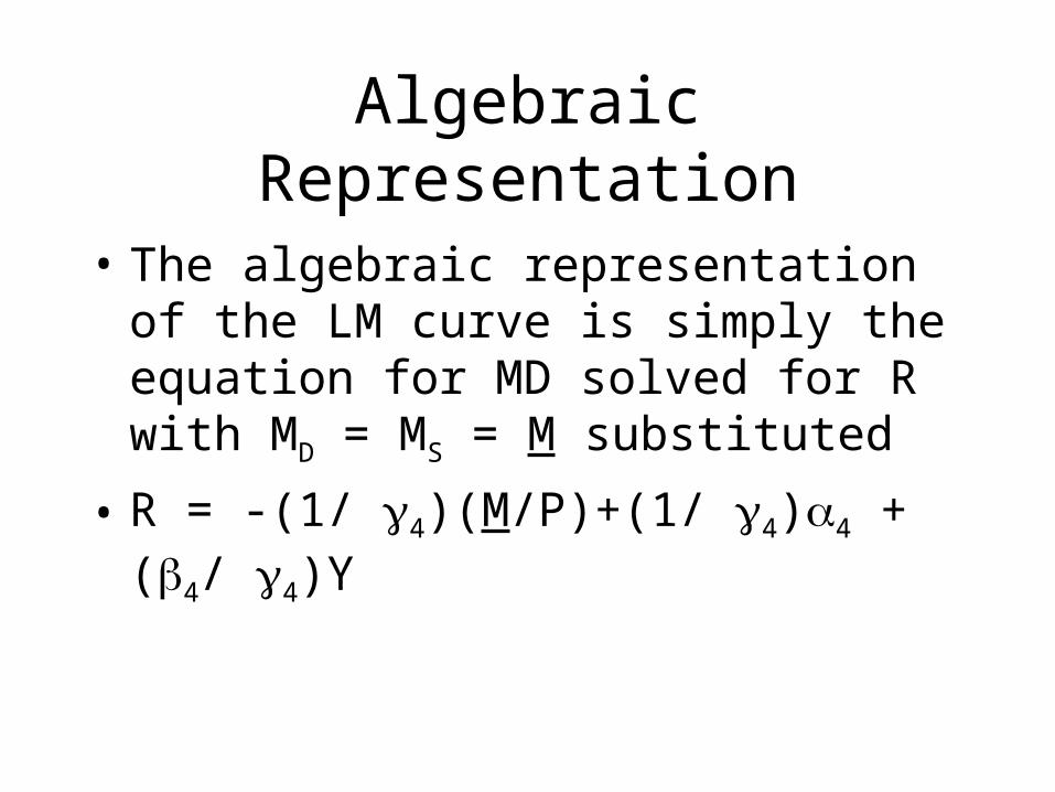
Algebraic Representation
• The algebraic representation of the LM curve is simply the equation for MD solved for R with MD = MS = M substituted
• R = -(1/ 4)(M/P)+(1/ 4)4 + (4/ 4)Y

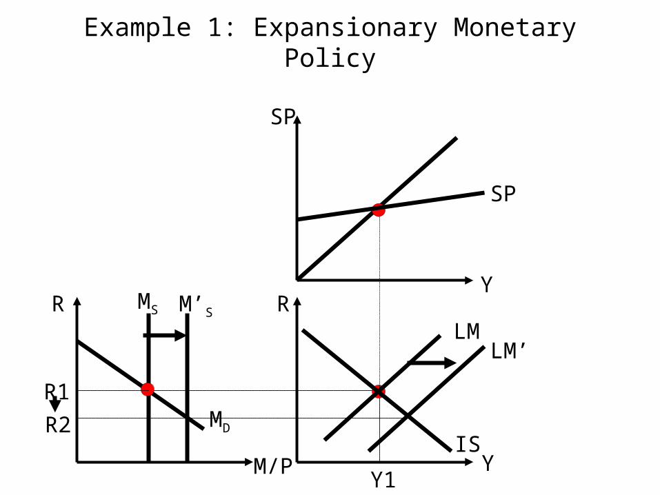
Shifts in the LM Curve: M < 0
• Begin at A. Suppose that the Fed “tightens” the money supply. M drops to M’, Ms shifts left; R rises.
R R
YM/P
MD
MS
A
Y1
A
F(Y1)
R1 B
LMM’S
R2

Shifts in the LM Curve: M < 0
• New equilibrium is B. Note Y1 is unchanged. LM shifts left.
• Contractionary, or “Tight” monetary policy shifts LM left
R R
YM/P
MD
MS
A
Y1
A
F(Y1)
R1 B
B LMM’S
R2
LM’
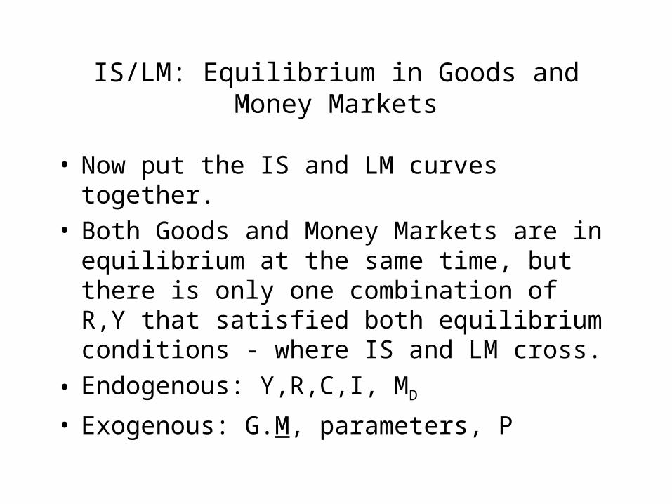
IS/LM: Equilibrium in Goods and Money Markets
• Now put the IS and LM curves together.• Both Goods and Money Markets are in
equilibrium at the same time, but there is only one combination of R,Y that satisfied both equilibrium conditions - where IS and LM cross.
• Endogenous: Y,R,C,I, MD
• Exogenous: G.M, parameters, P
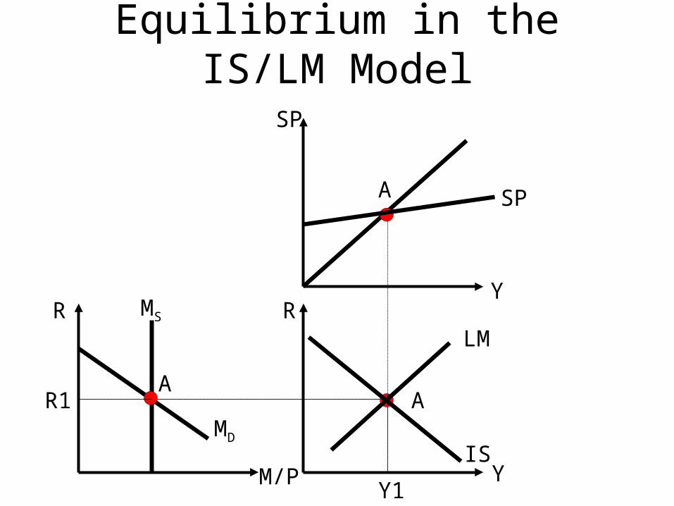
Equilibrium in the IS/LM Model
R R
YM/P
MD
MS
A
Y1
AR1
LM
Y
SP
SP
IS
A

Example 1: Expansionary Monetary Policy
R R
YM/P
MD
MS
Y1
R1
LM
Y
SP
SP
IS
M’S
Example 1: Expansionary Monetary Policy
R R
YM/P
MD
MS
Y1
R1
LM
Y
SP
SP
IS
M’S
R2
LM’

Example 1: Expansionary Monetary Policy
R R
YM/P
MD
MS
Y1
R1
LM
Y
SP
SP
IS
M’S
R2
LM’
Y2

Example 1: Expansionary Monetary Policy
R R
YM/P
MD
MS
Y1
R1
LM
Y
SP
SP
IS
M’S
R2
LM’
Y2
II’
SP’
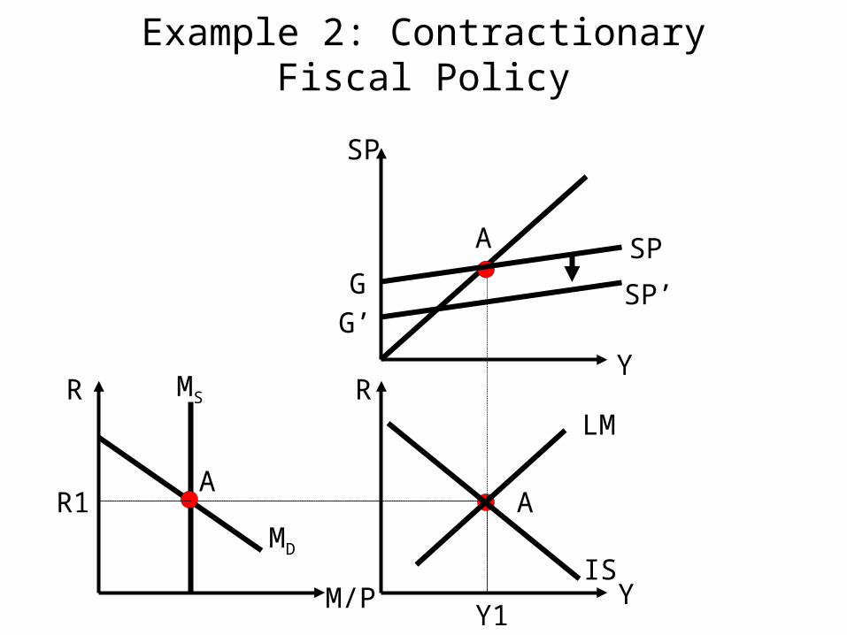
Example 2: Contractionary Fiscal Policy
R R
YM/P
MD
MS
A
Y1
AR1
LM
Y
SP
SP
IS
A
SP’G
G’

Example 2: Contractionary Fiscal Policy
R R
YM/P
MD
MS
A
Y1
AR1
LM
Y
SP
SP
IS
A
SP’G
G’
Y2IS’

Example 2: Contractionary Fiscal Policy
R R
YM/P
MD
MS
A
Y1
AR1
LM
Y
SP
SP
IS
A
SP’G
G’
Y2IS’MD’
R2

Price Adjustment in the IS/LM Model
• Rather than the complex price-adjustment process developed by Su, consider a simpler framework: Aggregate Supply/Aggregate Demand combined with the Phillips Curve.
• Has considerable explanatory power; leads to predictions that resemble what has happened in U.S. economic history.
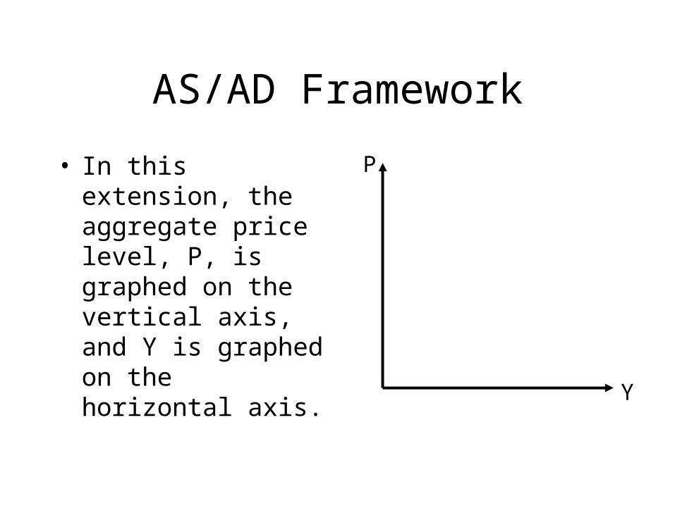
AS/AD Framework
• In this extension, the aggregate price level, P, is graphed on the vertical axis, and Y is graphed on the horizontal axis.
P
Y

Aggregate Supply
• The Aggregate Supply curve (AS) is a representation of “full employment” output (Yfe)
• This is the level of GDP when the economy is operating at capacity
• Yfe = Af(K,L*)
• Yfe responds only to changes in K.L*,A
P
Y
Yfe
AS

Aggregate Supply
• Yfe = Af(K,L*)
• Yfe responds only to changes in K.L*,A
• K>0 (growth in aggregate capital stock), A>0 (productivity growth) shift AS to the right. Long-run growth in capacity and productivity.
P
Y
Yfe
AS

Aggregate Demand
• The AD curve is simply a consequence of equilibrium in the goods and money markets
• Can be derived easily from IS/LM model
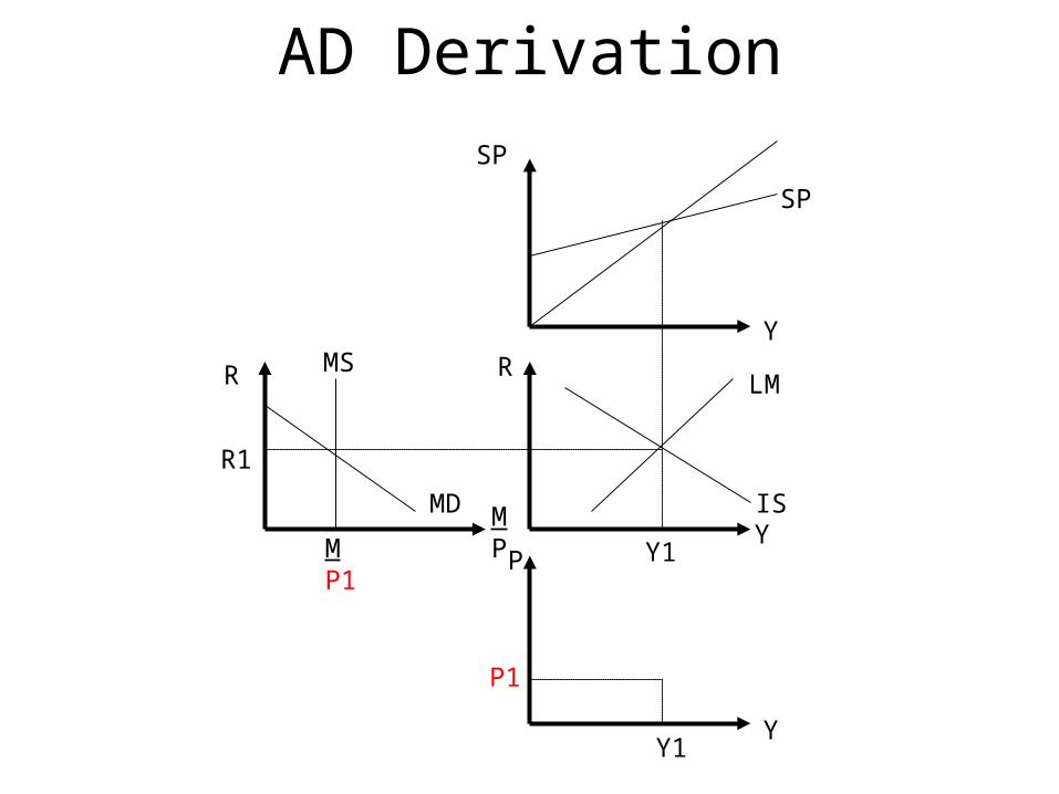
AD Derivation
R
Y
SP
P
MS
MD
MP1
MP
R
Y
Y
R1
Y1
LM
IS
SP
Y1
P1

AD Derivation
R
Y
SP
P
MS
MD
MP1
MP
R
Y
Y
R1
Y1
LM
IS
SP
Y1
P1
MS’
MP2
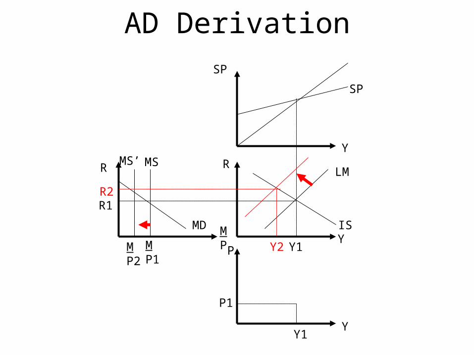
AD Derivation
R
Y
SP
P
MS
MD
MP1
MP
R
Y
Y
R1
Y1
LM
IS
SP
Y1
P1
MS’
MP2
R2
Y2

AD Derivation
R
Y
SP
P
MS
MD
MP1
MP
R
Y
Y
R1
Y1
LM
IS
SP
Y1
P1
MS’
MP2
R2
Y2
Y2
P2
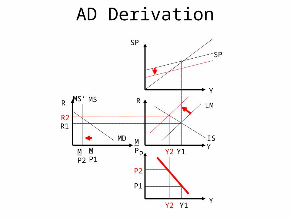
AD Derivation
R
Y
SP
P
MS
MD
MP1
MP
R
Y
Y
R1
Y1
LM
IS
SP
Y1
P1
MS’
MP2
R2
Y2
Y2
P2

Algebraic Representation of AD
• R = -(1/ 4)(M/P)+(1/ 4)4 + (4/ 4)Y
– LM Curve
• R = (1/2)(1 - 1t0+2+G) - (1/2)(1-1(1-t1)-2)Y– IS Curve
• Set IS=LM• Solve for P

Actual GDP vs. Potential
• In this framework, actual GDP is the Y where the horizontal price line cuts the AD curve
• The difference between actual and potential GDP (Y* - Yfe) is called “GDP Gap”
P
YYfe
AS
AD
P1
Y*
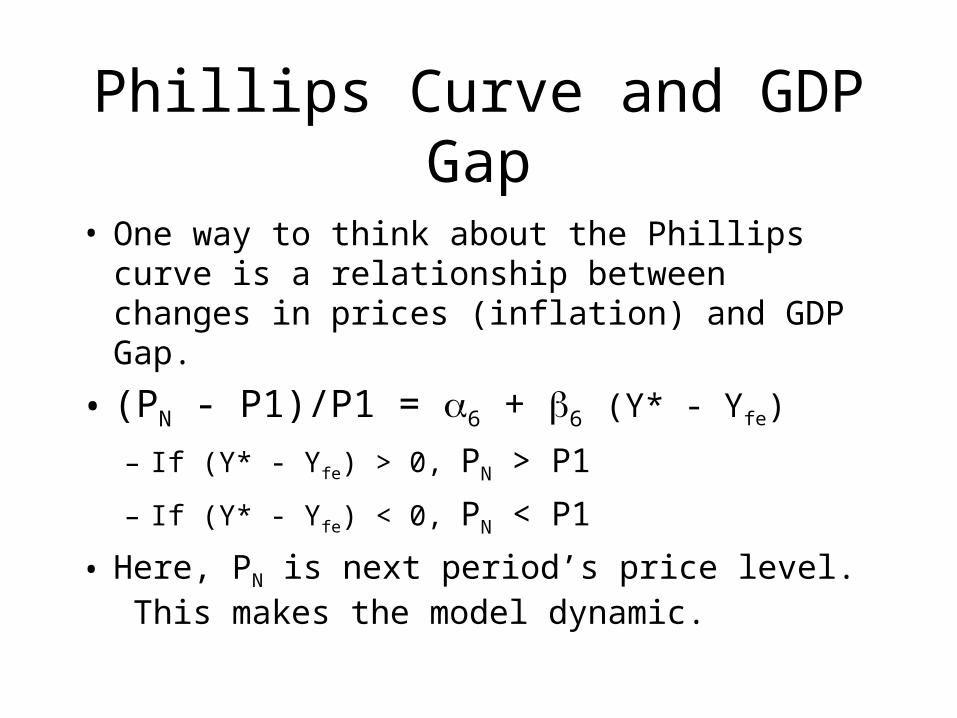
Phillips Curve and GDP Gap
• One way to think about the Phillips curve is a relationship between changes in prices (inflation) and GDP Gap.
• (PN - P1)/P1 = 6 + 6 (Y* - Yfe)
– If (Y* - Yfe) > 0, PN > P1
– If (Y* - Yfe) < 0, PN < P1
• Here, PN is next period’s price level. This makes the model dynamic.

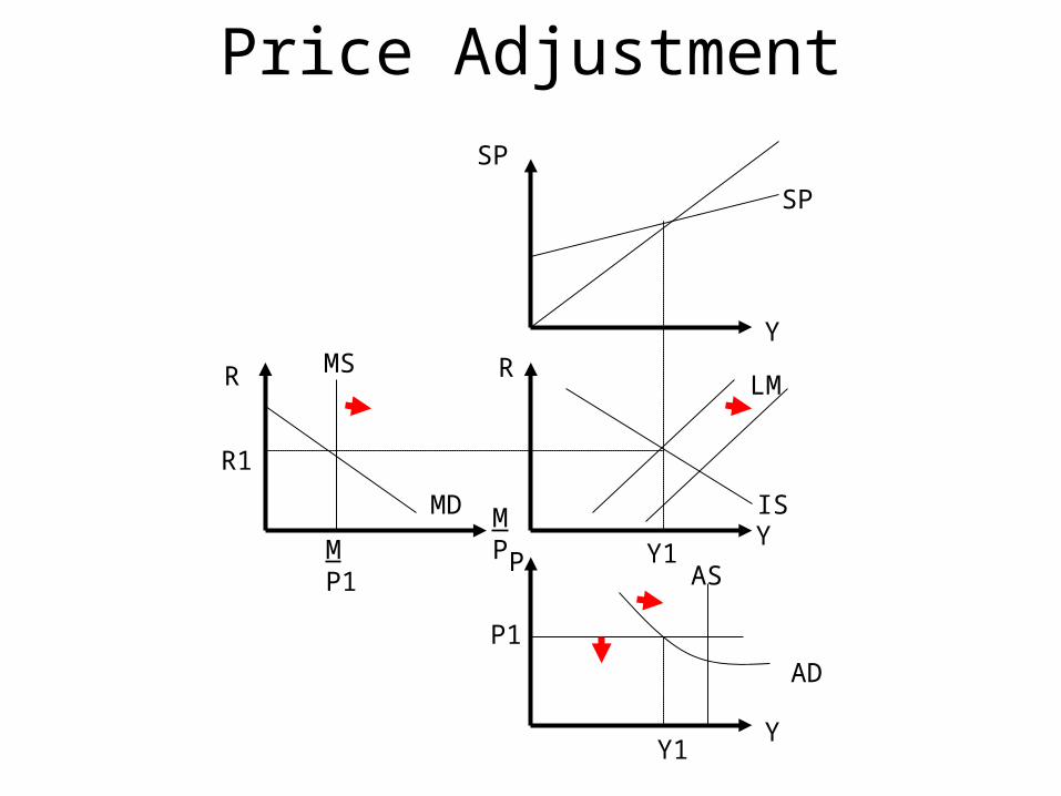
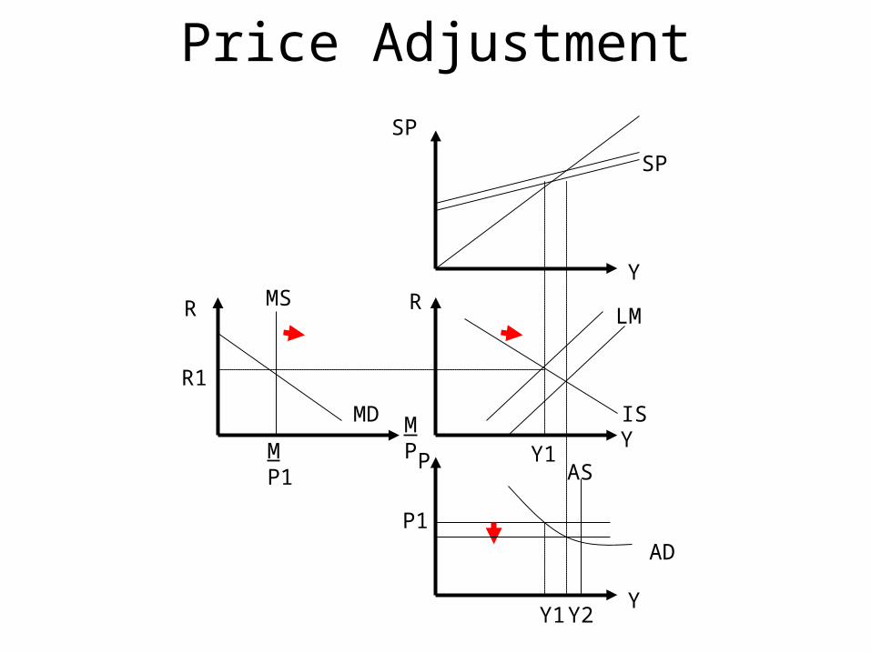
AS/AD in Action - Price Adjustment
• Start out with negative GDP gap.
• PN<P1 but how?
• Affects money supply-LM-AD, in that order.

Price Adjustment
R
Y
SP
P
MS
MD
MP1
MP
R
Y
Y
R1
Y1
LM
IS
SP
Y1
P1
AS
AD

Price Adjustment
R
Y
SP
P
MS
MD
MP1
MP
R
Y
Y
R1
Y1
LM
IS
SP
Y1
P1
AS
AD

Price Adjustment
R
Y
SP
P
MS
MD
MP1
MP
R
Y
Y
R1
Y1
LM
IS
SP
Y1
P1
AS
AD

Price Adjustment
R
Y
SP
P
MS
MD
MP1
MP
R
Y
Y
R1
Y1
LM
IS
SP
Y1
P1
AS
AD
Price Adjustment
R
Y
SP
P
MS
MD
MP1
MP
R
Y
Y
R1
Y1
LM
IS
SP
Y1
P1
AS
AD
Price Adjustment
R
Y
SP
P
MS
MD
MP1
MP
R
Y
Y
R1
Y1
LM
IS
SP
Y1
P1
AS
AD
Y2