review of chemiluminescence as an optical diagnostic tool
TRANSCRIPT

Purdue UniversityPurdue e-Pubs
Open Access Theses Theses and Dissertations
January 2015
Review of Chemiluminescence as an OpticalDiagnostic Tool for High Pressure UnstableRocketsTristan Latimer FullerPurdue University
Follow this and additional works at: https://docs.lib.purdue.edu/open_access_theses
This document has been made available through Purdue e-Pubs, a service of the Purdue University Libraries. Please contact [email protected] foradditional information.
Recommended CitationFuller, Tristan Latimer, "Review of Chemiluminescence as an Optical Diagnostic Tool for High Pressure Unstable Rockets" (2015).Open Access Theses. 1176.https://docs.lib.purdue.edu/open_access_theses/1176

Graduate School Form 30Updated 1/15/2015
PURDUE UNIVERSITYGRADUATE SCHOOL
Thesis/Dissertation Acceptance
This is to certify that the thesis/dissertation prepared
By
Entitled
For the degree of
Is approved by the final examining committee:
To the best of my knowledge and as understood by the student in the Thesis/Dissertation Agreement, Publication Delay, and Certification Disclaimer (Graduate School Form 32), this thesis/dissertation adheres to the provisions of Purdue University’s “Policy of Integrity in Research” and the use of copyright material.
Approved by Major Professor(s):
Approved by:Head of the Departmental Graduate Program Date
Tristan L. Fuller
REVIEW OF CHEMILUMINESCENCE AS AN OPTICAL DIAGNOSTIC TOOL FOR HIGH PRESSURE UNSTABLEROCKETS
Master of Science in Chemical Engineering
William E. AndersonChair
Robert P. Lucht
Stephen D. Heister
Carson D. Slabaugh
William E. Anderson
Weinong W. Chen 7/24/2015

REVIEW OF CHEMILUMINESCENCE AS AN OPTICAL DIAGNOSTIC TOOL IN HIGH PRESSURE UNSTABLE COMBUSTORS
A Thesis
Submitted to the Faculty
of
Purdue University
by
Tristan L. Fuller
In Partial Fulfillment of the
Requirements for the Degree
of
Master of Science
August 2015
Purdue University
West Lafayette, Indiana

ii
ACKNOWLEDGEMENTS
I would like to thank Professors Anderson and Lucht for giving me guidance throughout this
project.
Michael Bedard and Swanand Sardeshmukh contributed greatly in the development of the
optical model, so I would like to give them my sincerest thanks.
I would also like to thank my colleagues Carson Slabaugh, Zach Hallum, Cheng Huang, Rohan
Gejji and Matt Wierman for their help towards the finer details of this project and their effort
towards assisting me with presentation of the material.
Finally I would like to thank my parents for their support, for I would not have the opportunity
to work on this project if it were not for them. Thank you.

iii
TABLE OF CONTENTS
Page
LIST OF FIGURES ................................................................................................................. vii
ABSTRACT ............................................................................................................................ xvi
1. INTRODUCTION ............................................................................................................. 1
1.1 Background ...................................................................................................................... 1
1.2 Objectives ........................................................................................................................ 2
1.3 Thesis Chapters Rundown ............................................................................................... 3
2. REVIEW ........................................................................................................................... 4
2.1 Ideal Gases ....................................................................................................................... 4
2.2 Combustion Instability and High Pressure Systems ........................................................ 6
2.2.1 Combustion Instabilities [4] ..................................................................................... 6
2.2.2 Screeching – Thermoacoustic Combustion Instabilities .......................................... 7
2.2.3 Heat Release Modes ................................................................................................. 8
2.3 Chemiluminescence and Chemistry ................................................................................ 9
2.3.1 Chemistry Mechanisms ............................................................................................ 9
2.3.2 Elementary Reactions [5] ......................................................................................... 9
2.3.3 Collision Theory ..................................................................................................... 10
2.3.4 Free Radicals .......................................................................................................... 12
2.3.5 Reaction Kinetics ................................................................................................... 13

iv
Page
2.3.6 Exothermic Reactions ............................................................................................ 16
2.4 Detailed Chemical Kinetics Models .............................................................................. 17
2.4.1 GRI Mech 3.0 ......................................................................................................... 17
2.4.2 Reduced Chemical Kinetics Models ...................................................................... 18
2.4.3 Lifetimes of Chemiluminecence and Excited Species ........................................... 19
2.4.4 Chemical Kinetic Mechanism Augmentation for Excited Species ........................ 20
2.5 Use of Chemiluminescent Species in Reacting Flow .................................................... 21
2.5.1 Chemiluminescent Species Mechanism Models .................................................... 21
2.5.2 Chemiluminescent Species as Possible Quantifiable Markers of Flame Properties
......................................................................................................................................... 29
2.6 Spectroscopy .................................................................................................................. 32
2.6.1 Optics ..................................................................................................................... 32
2.6.2 Structure of Internal Energy Modes of Molecules ................................................. 39
2.6.3 Emission, Absorption and Stimulated Emission .................................................... 50
2.6.4 Spectra of Emissions .............................................................................................. 60
2.7 Specific Spectroscopic Data Regarding OH and CH .................................................... 62
3. APPROACH ................................................................................................................... 64
3.1 Experimental Setup........................................................................................................ 64
3.2 Optical Model ................................................................................................................ 67
3.2.1 Physical Mechanisms in Model .............................................................................. 68
3.2.2 Model Construction ................................................................................................ 76
3.2.3 Normalized Spectrum Line Profile Estimation ...................................................... 92

v
Page
3.2.4 Numerical Considerations ...................................................................................... 96
3.3 Summary of Assumptions and Constants ...................................................................... 97
3.4 Model Verification Process ......................................................................................... 100
3.4.1 Example of Analytical Absorption Calculation ................................................... 100
3.4.2 Model Sensitivity ................................................................................................. 103
3.4.3 Error Estimates ..................................................................................................... 109
4. VERIFICATION DATA ............................................................................................... 111
4.1 Effect of Line Broadening on Signal Strength ............................................................ 111
4.2 Sensitivity Study .......................................................................................................... 113
4.2.1 Transmissivity with Respect to Number Density ................................................. 113
4.2.2 Sensitivity to Optical Path Length ....................................................................... 116
4.2.4 Sensitivity to Doppler Linewidth (Temperature) ................................................. 121
4.3 Error Estimation .......................................................................................................... 124
4.3.1 Data Initialisation from CFD ................................................................................ 124
4.3.2 Uncorrected Emission .......................................................................................... 125
4.3.3 Resultant Emission and Absorption ..................................................................... 127
4.3.4 Example Calculation of Error Propagation .......................................................... 129
5. RESULTS ..................................................................................................................... 130
5.1 Uncorrected Spectral Output for OH* and CH* .......................................................... 130
5.2 Resultant Emission of OH* and CH* Corrected for Absorption ................................. 133
5.3 Time Averaged Spectra ............................................................................................... 136

vi
Page
5.4 Temporal Measure of Signal Transmission ................................................................. 139
5.5 Spatial Measure of Signal Transmission ..................................................................... 143
5.6 Number Density Correlation ....................................................................................... 149
6. CONCLUSION AND SUMMARY .............................................................................. 155
6.1 Experimental and Numerical Spectra Comparison ...................................................... 155
6.2 OH* Emissions and Optical Density ........................................................................... 156
6.3 CH* Emissions and Optical Density ........................................................................... 157
6.4 OH* and CH* as Markers for Heat Release in the CVRC .......................................... 158
6.5 OH* and CH* as Markers for Heat Release in the General Case ................................ 159
6.6 Future Work ................................................................................................................. 159
REFERENCES ...................................................................................................................... 161
APPENDICES
Appendix A – Detailed Chemistry Mechanisms ............................................................... 168
1. GRI Mech 3.0 (Oxygen based oxidation only) ...................................................... 168
2. Chemiluminescence Augmentation to GRI Mech 3.0 ........................................... 177
Appendix B – Data and Plots ............................................................................................ 179
Appendix C – Subroutines and Logical Map .................................................................... 200
vii
LIST OF FIGURES
Figure Page
Figure 1: Collision volume swept out by a molecule interacting with identical molecules, with
diameter σ [5]. .......................................................................................................................... 11
Figure 2: Valence Electron Configurations for Ions and Radicals Involving Oxygen [6]. ...... 13
Figure 3: Potential Energy Curves for a) Exothermic Reactions and b) Endothermic Reactions
[7]. ............................................................................................................................................ 14
Figure 4: Effect of Molecule Orientation during Collision on Chemical Reactions [7]. ......... 15
Figure 5: Fully Compressed Molecule Depicted as an Anharmonic Oscillator Vibrating at an
Energy Level 𝐸𝐸3 [8]. ................................................................................................................ 17
Figure 6: High Temperature Reaction Pathway Diagram for the Combustion of Methane at
T=2200K. Reaction number numbers refer to Appendix A, and reaction rates are shown in
parentheses. For example, 3.3-7 implies 3.3 × 10 − 7𝑔𝑔𝑔𝑔𝑔𝑔𝑔𝑔𝑔𝑔𝑔𝑔3 − 𝑠𝑠 [5]. .............................. 19
Figure 7: Reaction Pathway Analysis of Premixed Methane-Air Combustion Showing the
Formation of Chemiluminescent Species [25]. ........................................................................ 25
Figure 8: Numerical Prediction of the Production of OH* in Methane-Air Combustion at
Various Pressures and Preheat Conditions [22]. ...................................................................... 26
Figure 9: Numerical Prediction of the Production of CH* in Methane-Air Combustion at
Various Pressures and Preheat Conditions [22]. ...................................................................... 26
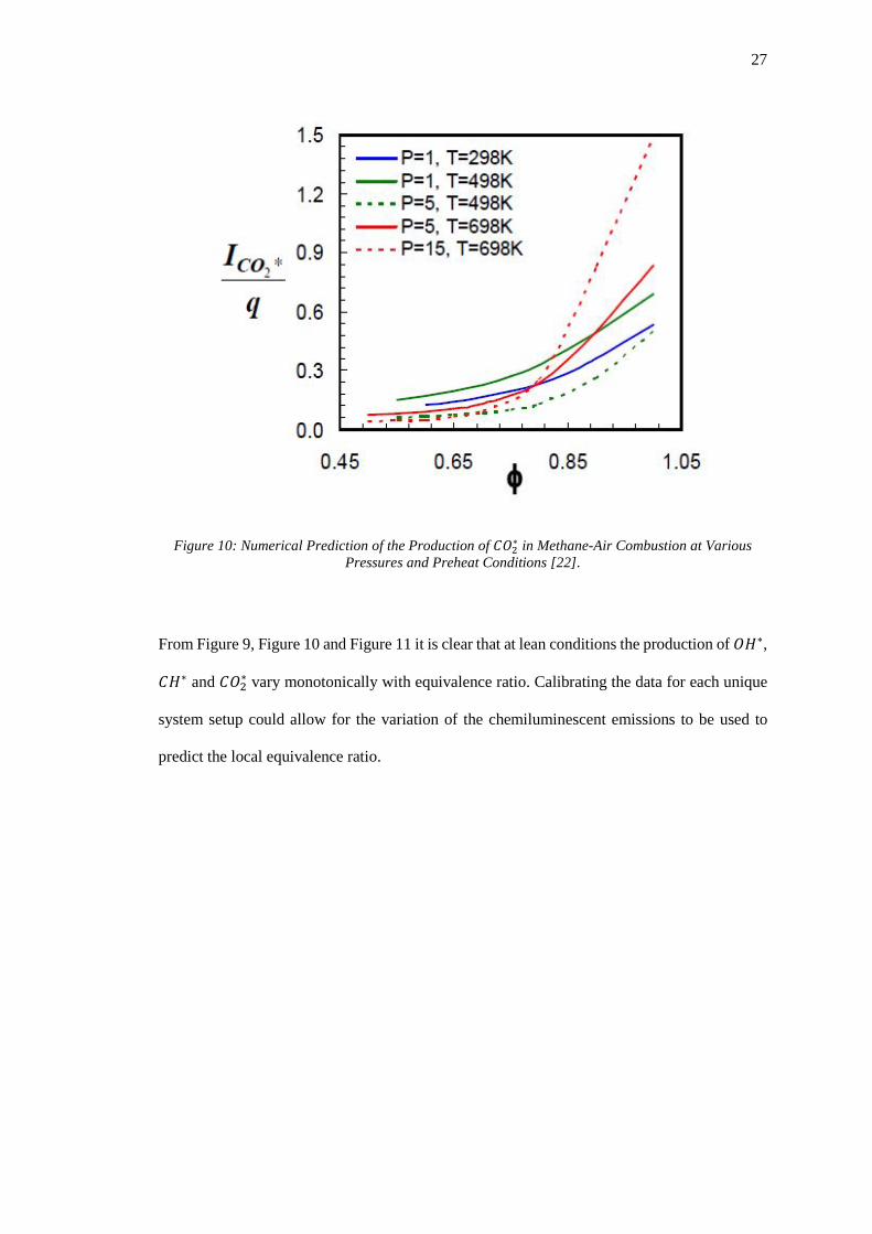
Figure 10: Numerical Prediction of the Production of 𝐶𝐶𝐶𝐶2 ∗ in Methane-Air Combustion at
Various Pressures and Preheat Conditions [22]. ...................................................................... 27

viii
Figure Page
Figure 11: Numerical Prediction of Product Recirculation Dependence of OH* (solid lines) and
CH* (lines with symbols) in lean (𝜙𝜙=0.7) methane-air flames [22]. ....................................... 28
Figure 12: Numerical Prediction of Strain Rate Dependence of OH* (solid lines) and CH* (lines
with symbols) in lean (ϕ=0.7) methane-air flames [22]. .......................................................... 29
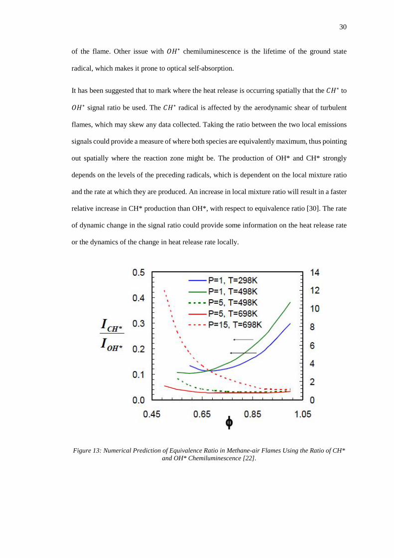
Figure 13: Numerical Prediction of Equivalence Ratio in Methane-air Flames Using the Ratio
of CH* and OH* Chemiluminescence [22]. ............................................................................ 30
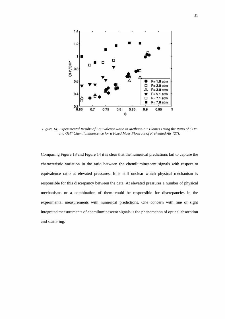
Figure 14: Experimental Results of Equivalence Ratio in Methane-air Flames Using the Ratio
of CH* and OH* Chemiluminescence for a Fixed Mass Flowrate of Preheated Air [27]. ...... 31
Figure 15: The Structure of an Oscillating Electromagnetic Field known as a Light Wave [31].
................................................................................................................................................. 32
Figure 16: The Analogy between a 2D Arc and the 3D Solid Angle [33]. .............................. 34
Figure 17: Polarization Induced in a Molecule in the Presence of an Externally Applied Electric
Field [35]. ................................................................................................................................. 36
Figure 18: An Illustration of a Beam of Photons Passing through a Slab Conveying the Concept
of Absorption Cross Section [38]. ........................................................................................... 40
Figure 19: Discrete Structure of the Potential Energy Levels Corresponding to the Different
Modes of Internal Energy Storage of a Molecule [38]. ........................................................... 41
Figure 20: Space Quantization of the Electron Orbital Angular Momentum and Spin within an
Atom in the Presence of an Externally Applied Magnetic Field [35]. ..................................... 43
Figure 21: Space Quantization of the Electron Orbital Angular Momentum and Spin within a
Molecule in the Presence of an Externally Applied Magnetic Field, 𝒍𝒍 [35]. ........................... 46
Figure 22: Orientation of the Angular Momentum Vectors for both Hund's (a, top) and (b,
bottom) Coupling [35]. ............................................................................................................ 48

ix
Figure Page
Figure 23: Franck–Condon principle energy diagram. Since electronic transitions are very fast
compared with nuclear motions, vibrational levels are favored when they correspond to a
minimal change in the nuclear coordinates. The potential wells are shown favouring v = 0 and
v = 2. ........................................................................................................................................ 52
Figure 24: Spring-Mass System Analogy for a Collision between a Molecule and a Particle
[39]. .......................................................................................................................................... 58
Figure 25: Experimental Setup and Modelled Domain Location of the CVRC (Continuously
Variable Resonance Combustor) – Courtesy: Michael J. Bedard. ........................................... 65
Figure 26: Spectroscopic Experimental Setup. The Zoomed in Bubble shows the Probe Volume
of Measurement. ...................................................................................................................... 66
Figure 27: Fibre Optic Port Design. ......................................................................................... 67
Figure 28: Computationally Modelled Domain relative to Experimental Setup. .................... 68
Figure 29: Discretized Form of the Beer-Lambert Law for Cell Centred Data. ...................... 69
Figure 30: Ray Traces and Acceptance Cone for a Multimode Fibre Optic Cable [50]. ......... 75
Figure 31: Orthogonal Axes of Symmetry for a Cone Intersecting a Cylinder; a Crude Analogy
of the Probe Volume within the Combustor Computational Domain. The Blue Line represents
the Axis of Symmetry for the Chamber Computational Domain and the Red Line represents the
Axis of Symmetry for the Probe Volume. ............................................................................... 76
Figure 32: Solid Angle Fraction Bias of the Discrete Data Points within the Probe Volume as
viewed from above. .................................................................................................................. 77
Figure 33: Ray Trace Analogy with Optimized Method for Finding Closest Points to Ray. The
Re Line represents the Ray, the Blue Dots represent the Cell Centred Discrete Points within the
Probe Volume and the Green Points are the Closest Points of the Probe Volume to the Ray. 78
Figure 34: Representation of the Annular Cell in 3D of an Axisymmetric 2D Cell in Plane. The
Axes of the Annular Cell are Arbitrary. ................................................................................... 80
x
Figure Page
Figure 35: Generalized Volume Approach to Quadrilateral Cross Sectioned Cell.................. 80
Figure 36: Cell Volume Distribution within Probe Volume for 1800 Revolutions of the 2D
Axisymmetric Computational Domain. ................................................................................... 83
Figure 37: Number Density Distribution of OH within Probe Volume. Shell 1 of 6. ............. 84
Figure 38: Number Density Distribution of OH within Probe Volume. Shell 2 of 6. ............. 84
Figure 39: Number Density Distribution of OH within Probe Volume. Shell 3 of 6. ............. 84
Figure 40: Number Density Distribution of OH within Probe Volume. Shell 4 of 6. ............. 84
Figure 41: Number Density Distribution of OH within Probe Volume. Shell 5 of 6. ............. 85
Figure 42: Number Density Distribution of OH within Probe Volume. Shell 6 of 6. ............. 85
Figure 43: Cell Volume Distribution per Shell within Probe Volume. Shell 1 of 6. ............... 85
Figure 44: Cell Volume Distribution per Shell within Probe Volume. Shell 2 of 6. ............... 85
Figure 45: Cell Volume Distribution per Shell within Probe Volume. Shell 3 of 6. ............... 86
Figure 46: Cell Volume Distribution per Shell within Probe Volume. Shell 4 of 6. ............... 86
Figure 47: Cell Volume Distribution per Shell within Probe Volume. Shell 5 of 6. ............... 86
Figure 48: Cell Volume Distribution per Shell within Probe Volume. Shell 6 of 6. ............... 86
Figure 49: Number Density Distribution of OH within Probe Volume. Shell 1 of 12. ........... 88
Figure 50: Number Density Distribution of OH within Probe Volume. Shell 3 of 12. ........... 88
Figure 51: Number Density Distribution of OH within Probe Volume. Shell 5 of 12. ........... 88
Figure 52: Number Density Distribution of OH within Probe Volume. Shell 7 of 12. ........... 88
Figure 53: Number Density Distribution of OH within Probe Volume. Shell 9 of 12. ........... 89
Figure 54: Number Density Distribution of OH within Probe Volume. Shell 11 of 12. ......... 89
Figure 55: Cell Volume Distribution per Shell within Probe Volume. Shell 1 of 12. ............. 89
Figure 56: Cell Volume Distribution per Shell within Probe Volume. Shell 3 of 12. ............. 89
Figure 57: Cell Volume Distribution per Shell within Probe Volume. Shell 5 of 12. ............. 90
Figure 58: Cell Volume Distribution per Shell within Probe Volume. Shell 7 of 12. ............. 90

xi
Figure Page
Figure 59: Cell Volume Distribution per Shell within Probe Volume. Shell 9 of 12. ............. 90
Figure 60: Cell Volume Distribution per Shell within Probe Volume. Shell 11 of 12. ........... 90
Figure 61: CH* Spectrally Integrated Emission of the Probe Volume as Approximated by
Varying Number of 1D Shells. The Green Line Represents the Running Mean of the Data as a
Function of Number 1D Shells. ............................................................................................... 91
Figure 62: OH* Spectrally Integrated Emission of the Probe Volume as Approximated by
Varying Number of 1D Shells. The Green Line Represents the Running Mean of the Data as a
Function of Number 1D Shells. ............................................................................................... 91
Figure 63: Emission Spectral Simulation of OH Emission at T=2400K and P=15atm. A Voigt
Line Shape was used, Doppler and Collisional Linewidths are approximately 0.03 and 0.98
𝑔𝑔𝑔𝑔 − 1 respectively [53]. ........................................................................................................ 95
Figure 64: Time Averaged Emission Spectrum from the CVRC Experiment. ........................ 95
Figure 65: Monochromatic and Broadened Absorption Lines for 𝑃𝑃1(1.5) Transition of OH for
a Number Density of 1021 𝑔𝑔− 3 and a Temperature of 2500K. ......................................... 112
Figure 66: Monochromatic and Broadened Absorption Lines for 𝑅𝑅1𝑎𝑎 + 𝑅𝑅1𝑏𝑏 (1.5) Transition
of CH for a Number Density of 1021 𝑔𝑔− 3 and a Temperature of 2500K. ....................... 112
Figure 67: Normalized Sensitivity of Transmissivity to Variation of the OH Ground State
Number Density for different Optical Path Lengths .............................................................. 114
Figure 68: Normalized Sensitivity of Transmissivity to Variation of the CH Ground State
Number Density for different Optical Path Lengths. ............................................................. 114
Figure 69: Absorption Sensitivity to Variations of Ground State Number Density of OH and
CH for an Optical Path Length of z = 0.045m. ...................................................................... 116
Figure 70: Variation in Absorption Sensitivity with Perturbations in the Optical Depth with
Varying Number Densities of OH. ........................................................................................ 117
xii
Figure Page
Figure 71: Variation in Absorption Sensitivity with Perturbations in the Optical Depth with
Varying Number Densities of CH. ......................................................................................... 117
Figure 72: Sensitivity of the Predicted Absorption due to Collisional Linewidth for OH.
Isometric View. ...................................................................................................................... 118
Figure 73: Sensitivity of the Predicted Absorption due to Collisional Linewidth for OH. Top
View ....................................................................................................................................... 119
Figure 74: Sensitivity of the Predicted Absorption due to Collisional Linewidth for CH.
Isometric View. ...................................................................................................................... 119
Figure 75: Sensitivity of the Predicted Absorption due to Collisional Linewidth for CH. Top
View. ...................................................................................................................................... 120
Figure 76: Sensitivity of the Predicted Absorption due to Perturbations in Temperature for OH.
Isometric View. ...................................................................................................................... 121
Figure 77: Sensitivity of the Predicted Absorption due to Perturbations in Temperature for OH.
Top View. .............................................................................................................................. 122
Figure 78: Sensitivity of the Predicted Absorption due to Perturbations in Temperature for CH.
Isometric View. ...................................................................................................................... 122
Figure 79: Sensitivity of the Predicted Absorption due to Perturbations in Temperature for CH.
Top View. .............................................................................................................................. 123
Figure 80: Uncorrected Radiant Power Emitted by OH* during an Oscillation within the CVRC.
............................................................................................................................................... 131
Figure 81: Uncorrected Radiant Power Emitted by CH* during an Oscillation within the CVRC.
............................................................................................................................................... 131
Figure 82: Uncorrected Combined Radiant Power Spectra Emitted by OH* and CH* during an
Oscillation within the CVRC. The OH* Spectra are Located on the Left Hand Side of the Plot
and the CH* Spectra are Located on the Right.The CH* spectra are multiplied x500. ......... 132
xiii
Figure Page
Figure 83: Absorption Corrected Radiant Power Emitted by OH* during an Oscillation within
the CVRC. .............................................................................................................................. 134
Figure 84: Absorption Corrected Radiant Power Emitted by CH* during an Oscillation within
the CVRC. .............................................................................................................................. 134
Figure 85: Absorption Corrected Combined Radiant Power Spectra Emitted by OH* and CH*
during an Oscillation within the CVRC. The OH* Spectra are Located on the Left Hand Side
of the Plot and the CH* Spectra are Located on the Right. The CH* spectra are multiplied x100.
............................................................................................................................................... 135
Figure 86: Uncorrected Time Averaged Spectrum of OH* during One Oscillation. ............ 137
Figure 87: Uncorrected Time Averaged Spectrum of CH* during One Oscillation. ............. 137
Figure 88: Uncorrected Time Averaged Combined Spectrum of OH* and CH* during One
Oscillation. ............................................................................................................................. 138
Figure 89: Absorption Corrected Time Averaged Combined Spectrum of OH* and CH* during
One Oscillation ...................................................................................................................... 138
Figure 90: Temporal Evolution of the Spectral Transmissivity of the CVRC Combustion
Medium within the Probe Volume for OH* during the Period of One Cycle. (Isometric View)
............................................................................................................................................... 140
Figure 91: Temporal Evolution of the Spectral Transmissivity of the CVRC Combustion
Medium within the Probe Volume for OH* during the Period of One Cycle. (Temporal View)
............................................................................................................................................... 140
Figure 92: Temporal Evolution of the Spectral Transmissivity of the CVRC Combustion
Medium within the Probe Volume for OH* during the Period of One Cycle. (Spectral View)
............................................................................................................................................... 141
xiv
Figure Page
Figure 93: Temporal Evolution of the Spectral Transmissivity of the CVRC Combustion
Medium within the Probe Volume for CH* during the Period of One Cycle. (Isometric View)
............................................................................................................................................... 142
Figure 94: Temporal Evolution of the Spectral Transmissivity of the CVRC Combustion
Medium within the Probe Volume for CH* during the Period of One Cycle. (Temporal View)
............................................................................................................................................... 142
Figure 95: Temporal Evolution of the Spectral Transmissivity of the CVRC Combustion
Medium within the Probe Volume for CH* during the Period of One Cycle. (Spectral View)
............................................................................................................................................... 143
Figure 96: Spatial Distribution of the Spectral Absorption Fraction of OH*in the Probe Volume
at the Time Interval 75𝜇𝜇𝑠𝑠. ...................................................................................................... 144
Figure 97: Spatial Distribution of the Spectral Absorption Fraction of OH*in the Probe Volume
at the Time Interval 375μs. .................................................................................................... 145
Figure 98: Spatial Distribution of the Spectral Absorption Fraction of OH*in the Probe Volume
at the Time Interval 625μs. .................................................................................................... 145
Figure 99: Spatial Distribution of the Spectral Absorption Fraction of CH*in the Probe Volume
at the Time Interval 75μs. ...................................................................................................... 147
Figure 100: Spatial Distribution of the Spectral Absorption Fraction of CH*in the Probe
Volume at the Time Interval 375μs. ...................................................................................... 147
Figure 101: Spatial Distribution of the Spectral Absorption Fraction of CH*in the Probe
Volume at the Time Interval 625μs. ...................................................................................... 148
Figure 102: Temporal Evolution of the Correlation between the Effect that the Volume
Averaged Number Density within the Probe Volume has on the Ability for the CVRC
Combustion Medium to Transmit the OH* Emission Spectrum. The Transmissivity of the
Combustion Medium is Plotted against the Axis on the Right. ............................................. 150

xv
Figure Page
Figure 103: Temporal Evolution of the Correlation between the Effect that the Volume
Averaged Number Density within the Probe Volume has on the Ability for the CVRC
Combustion Medium to Transmit the CH* Emission Spectrum. The Transmissivity of the
Combustion Medium is Plotted against the Axis on the Right. ............................................. 150
Figure 104: Cross Section of 𝐶𝐶𝐶𝐶2 over the Spectrum of Interest for Different Temperatures.
............................................................................................................................................... 153
Figure 105: Transmissivity of 𝐶𝐶𝐶𝐶2 over the Spectrum of Interest for Different Temperatures.
............................................................................................................................................... 153
Figure 106: Transmissivity of 𝐶𝐶𝐶𝐶2 over the Spectrum of Interest for Different Number
Densities. ................................................................................................................................ 154
xvi
ABSTRACT
Fuller, Tristan L. MSAAE, Purdue University, August 2015. Review of Chemiluminescence as an Optical Diagnostic Tool in High Pressure Unstable Rockets. Major Professor: William E. Anderson.
The purpose of this project was to investigate the effects of optical absorption on line-of-sight
integrated chemiluminescence measurements in high pressure rockets. The use of
chemiluminescent emissions has been used in the past in an effort to characterise the flame
reaction zone and the corresponding heat release, however most efforts have been with low
pressure or atmospheric flames. Chemiluminescent measurements have been used in the case
of the Continuously Variable Resonant Combustor (CVRC) in an attempt to validate a CFD
simulation of the same system, although the CVRC operates at a higher pressure. For higher
pressure flames it is unclear if such measurements are valid. To bridge the gap between the
experimental and numerical data a spectroscopic model was created to study the validity of
chemiluminescent based measurements in the CVRC. It was found that the CVRC combustion
medium is optically opaque for the chemiluminescent emissions produced by OH* and
optically transparent for the chemiluminescent emissions produced by CH*. Unfortunately, the
emissions produced by CH* are largely influenced by the emissions produced by 𝐶𝐶𝐶𝐶2∗. As such,
both OH* and CH* are poor indicators of the heat release in the CVRC and therefore
chemiluminescence measurements are not useful in validating the CVRC CFD simulation.

1
1. INTRODUCTION
1.1 Background
Chemiluminescence measurement is an optical diagnostic technique devised to provide insight
into reacting flows at low cost and minimal complexity. The technique involves line-of-sight
measurement of the radiative emissions from electronically excited radicals resulting directly
from exothermic reactions with high energy output within the main reaction zone within a
flame.
The technique has been championed by researchers since the 1950’s, but until recently the
technique has not gained much interest. Lately, there has been an increased interest toward the
radiative emissions from the chemiluminescent species CH*, OH*, 𝐶𝐶2∗ and 𝐶𝐶𝐶𝐶2∗ within the
flames of hydrogen/oxygen and hydrocarbon/oxidizer combustors.
There have been numerous investigations, experimental and numerical, into the validity of these
chemiluminescent species as markers for the zone of energy release and the corresponding
dynamic trends associated with the measurements of the radiation emitted from these species.
The use of chemiluminescence as a quantitative diagnostic tool has also been investigated.
From these investigations there has been a growing concern of how the emitted radiation from
these chemiluminescent species may be affected by the presence of ground state radicals with
the ability to absorb the radiation before it is measured by an external observer. This poses a
serious problem for the technique involving line-of-sight integrated measurements of the

2
radiation. The concern is even greater for combustors which have much higher pressures than
ambient conditions, and even more so when the technique is applied to thermoacoustically
unstable combustion systems. In thermoacoustic instabilities the acoustic modes (pressure
oscillations) couple with the heat release modes of combustion and resonate. The resonance
results in exceedingly large pressure waves and enhanced heat transfer to the combustor wall,
both effects can cause catastrophic failure of the system. Currently there is much insight into
the acoustic modes within the oxidizer post/s and chamber sections of a rocket. The main piece
of the puzzle that is not known is the dynamics of the heat release modes; how they physically
couple and whether the pressure oscillations are a result of the heat release modes or vice versa.
Research involving combustion instabilities could use the local emissions from the
chemiluminescent species to gather data regarding the nature and characteristics of the heat
release and its dynamics. Using specific excited chemical species as markers for the heat release
spatially and temporally, a map of the energy release and the consequences thereof can be
constructed.
In order to make conclusions regarding the heat release using chemiluminescent measurements
there needs to be a certain level of confidence that the measured data is valid with respect to
the heat release within the flame. To compare the numerically simulated conditions of the
combustor to the experimental optical data directly a connection between the different physical
mechanisms (gas state physics and spectroscopy) needs to be made.
1.2 Objectives
o Construct a model of the volume measured by the fibre optic probe in the
CVRC.
o Populate the probe volume with chemiluminescent emitting species predicted
by the CFD model.
o Evaluate whether 𝐶𝐶𝐻𝐻∗ and 𝐶𝐶𝐻𝐻∗ signals measured at the entrance to the fibre
optic probe can be used as validation data.

3
1.3 Thesis Chapters Rundown
Section 2: Review
This section provides a fundamental background geared towards understanding the production
and the spectroscopic physics of chemiluminescence species within a flame. The section begins
with the basic thermodynamics of gas states, progresses to the finer points of flame chemistry
and then focuses on the quantum mechanics and statistical thermodynamics of spectroscopy.
Section 3: Approach
This section describes the conceptual approach towards the physical mechanisms within the
CVRC combustor and the optical model construction. The details of the model construction
and the processes through which it is verified are highlighted in this section.
Section 4: Verification
This section shows the results of the verification methods. The basic spectroscopic physics and
the corresponding equations are probed to ensure stability and precision of the optical model.
This section also attempts to quantify and estimate the error or standard deviation of the results
relative to the error of the CFD model.
Section 5: Results
This section shows the output of the optical model. The output is the uncorrected emissions,
corrected emissions due to absorption, transmissivity of the combustion medium temporally
and spatially for OH* and CH*. The effects of 𝐶𝐶𝐶𝐶2 concentration on the absorption of the
radiation produced by OH* and CH* is also discussed in this section.

4
2. REVIEW
A fundamental approach is used in this literature review. It is meant to give the reader a
thorough background from the simplest of topics to more advanced concepts, all of which are
utilized in producing an optical model of the emissions from the CVRC combustion chamber.
The optical model serves as a bridge between the experimental and numerical approaches
towards chemiluminescence as a diagnostic tool for heat release characteristics within unstable
rocket combustors. Fundamental constants are often represented in this literature review with a
standard deviation; the uncertainty in the values will be used later in order to extrapolate the
models error and uncertainty in its predictions.
2.1 Ideal Gases
According to classical thermodynamics, in the case of a very low density gas the intermolecular
potential energy may be neglected. In such a case the particles are said to be independent of
each other and can be referred to as an ideal gas [1]. An ideal gas behaves according to the
relationship:
𝑃𝑃𝑃𝑃 = 𝑛𝑛𝑅𝑅𝑢𝑢𝑇𝑇 = 𝑔𝑔𝑅𝑅𝑇𝑇 (1)
In which 𝑃𝑃 is the gas pressure, 𝑃𝑃 is the volume in which the gas occupies, 𝑇𝑇 is the gas
temperature, 𝑛𝑛 is the number of mols in the gas, 𝑔𝑔 is the mass of the gas, ℳ is the molecular
mass of the gas and 𝑅𝑅𝑢𝑢 [2] is the universal gas constant. Note that 𝑅𝑅 and 𝑅𝑅𝑢𝑢 are related by,

5
𝑅𝑅 =𝑅𝑅𝑢𝑢ℳ
(2)
And,
𝑅𝑅𝑢𝑢 = 8.3144621 ± 0.0000075𝐽𝐽
𝑔𝑔𝑔𝑔𝑔𝑔.𝐾𝐾
From statistical thermodynamics, entropy (𝑆𝑆) is related to the total number of microstates (also
known as the thermodynamic probability and given by 𝑊𝑊) a gas may have through the
Boltzmann relation [3], given:
𝑆𝑆 = 𝑘𝑘𝐵𝐵ln (𝑊𝑊) (3)
Where 𝑘𝑘𝐵𝐵 [2] is the constant of proportionality, known as the Boltzmann’s constant. The
number of microstates is a representation of the number of possible energy states that a gas can
occupy in a specific state, or macrostate. In the case of an ideal gas where the number of
molecules per volume is relatively low, thus the number of particles available as compared to
the number of possible energy states and it would be rare to have energy state occupied by more
than one particle. This case is known as the dilute limit. In the case of the dilute limit it can be
shown using standard energy relations from classical thermodynamics, which the equation of
state from a statistical thermodynamics point of view, takes on the form shown below,
𝑃𝑃𝑃𝑃 = 𝑁𝑁𝑘𝑘𝐵𝐵𝑇𝑇 (4)
With,
𝑘𝑘𝐵𝐵 = (1.3806488 ± 0.0000013) × 10−23𝐽𝐽𝐾𝐾
The number density, the number of particles per volume is given by 𝑁𝑁.
𝑘𝑘𝐵𝐵 =𝑛𝑛𝑅𝑅𝑢𝑢𝑁𝑁
=𝑅𝑅𝑢𝑢𝑁𝑁𝐴𝐴
(5)
𝑁𝑁𝐴𝐴 = (6.02214129 ± 0.00000027) × 1023𝑔𝑔𝑔𝑔𝑔𝑔−1

6
Comparing the state relations from both classical and statistical thermodynamics it is easy to
see in Equation (5) that Boltzmann’s constant is quantitatively linked to the universal gas
constant, where Avogadro’s constant 𝑁𝑁𝐴𝐴 [2] acts as a scaling factor between macroscale and
microscale thermodynamics.
A gas may still be considered ideal even if it is not homogeneous, that is the gas is mixture of
various chemical species. If the gas mixture is at thermal equilibrium then by the Zeroth Law
of Thermodynamics the different gas species will also be at thermal equilibrium at the same
temperature. With that being said, each chemical species in gas phase contributes to the overall
state of the gas mixture. Since the gas and its components occupy the same volume the only
state properties that the gas species can attribute their state to the overall gas mixture state are
pressure and the number of particles of the gaseous specie. Each gaseous specie contributes
their pressure to the mixture, known as partial pressure. This can be directly linked to the
number of molecules of the species in the mixture; the fraction of the number of particles of the
gaseous species per total number of particles present in the gas mixture. This is known as mole
fraction and is given by:
Χ =𝑛𝑛𝑖𝑖∑𝑛𝑛
=𝑃𝑃𝑖𝑖∑𝑃𝑃
(6)
The mass fraction of a particular gas specie within the gas mixture can be extracted by
converting the number molecules into a mass property or density property, i.e.,
𝑌𝑌𝐴𝐴 = 𝑋𝑋𝐴𝐴 ×ℳ𝐴𝐴
ℳ𝑚𝑚𝑖𝑖𝑚𝑚=𝑔𝑔𝐴𝐴∑𝑔𝑔
=𝜌𝜌𝐴𝐴𝜌𝜌𝑡𝑡𝑡𝑡𝑡𝑡
(7)
2.2 Combustion Instability and High Pressure Systems
2.2.1 Combustion Instabilities [4]
Fluctuations in pressure, temperature and velocity are always present in a rocket combustor. If
the pressure fluctuations are below ±5% of the mean chamber pressure the rocket is said to

7
experience smooth combustion. The combustion is deemed unstable if the pressure fluctuations
exceed ±5% of the mean chamber pressure. There are three main types of combustion
instability based on the frequency range at which the oscillations occur.
The first type of combustion instability is referred to as “chugging” and occurs at a low
frequency range of 10-400Hz. The causal link of the combustion instability is the combustion
chamber and the propellant feed system, if not the entire vehicle. The second type of
combustion instability occurs at an intermediate frequency range of 400-1000Hz and is usually
referred to by one of these names: acoustic, “buzzing” or entropy waves. These combustion
instabilities are linked via mechanical vibrations of the propulsion structure, injector manifold
oscillations, flow eddies, fuel/oxidizer ratio fluctuations and propellant feed resonances. The
third form of combustion instability occurs at high frequencies above 1kHz. They are often
referred to as “screaming” or “screeching”. High frequency combustion instabilities are
thermoacoustic in nature; when pressure waves formed from combustion processes couple with
the chamber acoustic resonance properties.
2.2.2 Screeching – Thermoacoustic Combustion Instabilities
Because the energy content increases with frequency, screeching is the most destructive type
of combustion instability. It often happens that the instantaneous pressure peaks be around
twice the mean chamber pressure during the limit cycle of combustion instability. The high
pressure oscillations be destructive in a variety of ways; excitation of the vehicle structure
vibrational modes, low-cycle fatigue of the combustion chamber and components and
exceedance of the chamber material strength. Additionally the heat transfer to the combustor
walls is also magnified [4], sometimes on the order of a magnitude depending on the acoustic
mode excited. This may cause melting of the combustion chamber, nozzle throat and/or the
injector face of a rocket.
Generally, high frequency combustion instabilities are thought of as the coupling between the
acoustic resonance modes of the rocket chamber and the combustion heat release modes. It is
8
not entirely clear what mechanisms govern the nature of the combustion heat release modes,
but the more popular opinion is that the mixing process is enhanced in the presence of an
acoustic wave. The fluidic nature of the propellant injected into the chamber may also be
affected. In both hypotheses the local mixture ratios within the combustion chamber are
affected by the local pressure changes due to the acoustic waves.
The Rayleigh criterion is a method to evaluate the status of thermoacoustic instabilities based
on pressure and heat release rate perturbations. If the Rayleigh index is positive, where the heat
release rate oscillations are approximately in phase with the pressure oscillations, then driving
of thermoacoustic instability is said to occur. Conversely, if the Rayleigh index is negative,
where the heat release rate oscillations are approximately out of phase with the pressure
oscillations, then thermoacoustic damping occurs. The Rayleigh index is expressed as,
𝐺𝐺(𝑥𝑥) =1𝑇𝑇�𝑞𝑞′(𝑥𝑥, 𝑡𝑡)𝑝𝑝′(𝑥𝑥, 𝑡𝑡)𝑑𝑑𝑡𝑡
𝑇𝑇 (8)
2.2.3 Heat Release Modes
Since the nature of the heat release rate modes is poorly understood then it follows that high
frequency combustion instability is still now well understood. There has been a large effort
towards characterising the heat release rate and its modes, especially during instability. Direct
measurement of the heat release modes using thermocouples is limited with current technology
and materials. Any direct measurement device placed inside the flame reaction zone will melt
before any meaningful measurements could be taken. As such, there has been interest in the
spectroscopy of flames in order to gather meaningful data on the nature of heat release from
within a combustion zone.
Spectroscopic measurements involve the collection of optical data. There are many different
spectroscopic methods today, many of which employ the use of lasers. Another popular method
which is involved purely with the purpose of collecting data from the reactive heat release zone
is the measurement of chemiluminescent emissions.

9
2.3 Chemiluminescence and Chemistry
2.3.1 Chemistry Mechanisms
The overall combustion reaction of a mole of fuel with a moles of oxidizer to form b moles of
products can be expressed by the global reaction mechanism [5]:
𝐹𝐹𝐹𝐹 + 𝑎𝑎𝐶𝐶𝑥𝑥 → 𝑏𝑏𝑃𝑃𝑏𝑏 (9)
The global reaction mechanism expressed by Equation (9) may sometimes be used to
approximate and solve simpler problems, however for more complex problems where a more
thorough understanding of the process is needed it is not sufficient. It is unrealistic to expect
that the formation of the products is an immediate and direct result of the reaction between the
molecules of the fuel and oxidiser; as this would usually consist of several molecular bonds
being severed and formed in a single process [5]. In reality a number, usually many, sequential
processes occur involving many intermediate species during a combustion reaction. The
fundamental reaction mechanisms which occur during the combustion process are called
elementary reactions.
2.3.2 Elementary Reactions [5]
An elementary reaction is a fundamental chemical reaction involving at most two reacting
species. Elementary reactions can be further subdivided into three groups: unimolecular,
bimolecular and termolecular. Unimolecular reactions involve a single chemical species
undergoing a rearrangement (isomerization or decomposition) to for form one or two products,
as shown below,
𝐴𝐴 → 𝐵𝐵 (10)
or,
𝐴𝐴 → 𝐵𝐵 + 𝐶𝐶. (11)

10
Bi molecular reactions are the most common form of elementary reactions during a combustion
process; two reactant molecules collide and form two product molecules. This reaction is
expressed as,
𝐴𝐴 + 𝐵𝐵 → 𝐶𝐶 + 𝐷𝐷 (12)
Termolecular reactions involve three reactant species, where only two of the three reactants
chemically react. The third species usually denoted by M serves as a third body to or from
which energy is transferred, the energy is usually manifested as kinetic energy. The general
reaction can be expressed as,
𝐴𝐴 + 𝐵𝐵 + 𝑀𝑀 → 𝐶𝐶 +𝑀𝑀 (13)
Examples of each type of these reactions are given below [5].
Elementary Reaction General Form
Unimolecular 𝐶𝐶2𝐻𝐻4 → 𝐻𝐻2 + 𝐶𝐶2𝐻𝐻2 (14)
Bimolecular 𝐶𝐶2 + 𝐶𝐶𝐶𝐶 → 𝐶𝐶 + 𝐶𝐶𝐶𝐶2 (15)
Termolecular 𝐻𝐻 + 𝐻𝐻 + 𝑀𝑀 → 𝐻𝐻2 + 𝑀𝑀 (16)
For bi- and termolecular reactions to occur there needs to be some physical interaction between
the molecules. The interaction between the molecules is usually in the form of collisions, which
are usually elaborate upon as part of the theory of gases.
2.3.3 Collision Theory
There are a number of gas theory models predicting the effective interaction distance between
molecules. The “billiard ball” model analogizes the interaction between molecules to the
collision of hard spheres. The kinetic theory of gases is a model for the behaviour of gases
which uses the “billiard ball” approach. Using kinetic theory of gases in conjunction with Fick’s
law for mass diffusion the mean free path and collision frequency per unit area are derived [5]:
11
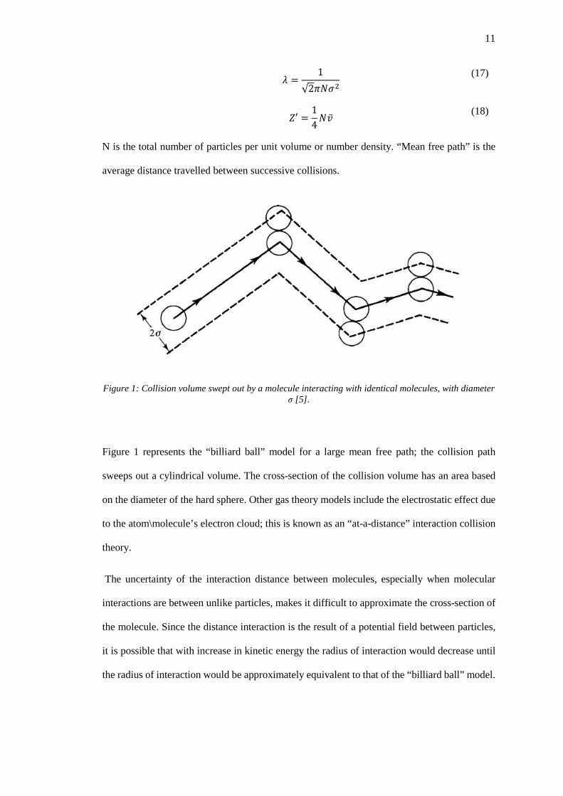
𝜆𝜆 =1
√2𝜋𝜋𝑁𝑁𝜎𝜎2
(17)
𝑍𝑍′ =14𝑁𝑁�̅�𝑣
(18)
N is the total number of particles per unit volume or number density. “Mean free path” is the
average distance travelled between successive collisions.
Figure 1: Collision volume swept out by a molecule interacting with identical molecules, with diameter σ [5].
Figure 1 represents the “billiard ball” model for a large mean free path; the collision path
sweeps out a cylindrical volume. The cross-section of the collision volume has an area based
on the diameter of the hard sphere. Other gas theory models include the electrostatic effect due
to the atom\molecule’s electron cloud; this is known as an “at-a-distance” interaction collision
theory.
The uncertainty of the interaction distance between molecules, especially when molecular
interactions are between unlike particles, makes it difficult to approximate the cross-section of
the molecule. Since the distance interaction is the result of a potential field between particles,
it is possible that with increase in kinetic energy the radius of interaction would decrease until
the radius of interaction would be approximately equivalent to that of the “billiard ball” model.

12
Temperature is the measure of the mean translational kinetic energy of an ensemble of particles.
From the kinetic theory of gases the ideal relationship between temperature and kinetic energy
in three dimensions, assuming a Maxwell-Boltzmann distribution can be expressed as,
𝐸𝐸𝑇𝑇 =12𝑔𝑔𝑣𝑣𝑟𝑟𝑚𝑚𝑟𝑟
2 =32𝑘𝑘𝐵𝐵𝑇𝑇
(19)
where m is the particle mass, 𝑣𝑣𝑟𝑟𝑚𝑚𝑟𝑟 is the root-mean-square particle velocity and T is the mean
translational temperature. The expected or mean velocity of the particles can also be expressed
through kinetic gas theory by [5],
⟨𝑣𝑣⟩ = �̅�𝑣 = �8𝑘𝑘𝐵𝐵𝑇𝑇
𝜋𝜋𝑔𝑔
(20)
Now, from Figure 1 and Equations 18 and 20, the collision frequency for identical molecules,
assuming a Maxwellian distribution of particle velocities can be expressed as
𝜈𝜈𝐶𝐶 = √2𝑁𝑁�̅�𝑣𝜋𝜋𝜎𝜎2 (21)
𝜋𝜋𝜎𝜎2 → 𝜎𝜎𝑒𝑒𝑒𝑒𝑒𝑒 (22)
To adjust for a variation in the collision frequency due to at-a-distance interaction and different
collision partners, the cross-sectional area can be augmented or replaced by a more accurate
value shown in Equation 22. In the case with molecules where it is difficult to calculate the
cross-sectional area it is common for empirical data to be used for specific gas state properties.
2.3.4 Free Radicals
During chemical reactions elementary reactions occur. An elementary reaction usually involves
the break or formation of a single molecular bond; the result of this reaction is the formation of
intermediate species. These intermediate species do not usually exist at normal ambient
conditions because they tend to be very reactive. The high reactivity of the intermediate species
is because of at least one unpaired electron in the valence shell of at least one of the atoms. A
molecular species with an unpaired electron in its valence shell is called a radical or free radical;
an example is the hydroxyl radical shown below in Figure 2.

13
Figure 2: Valence Electron Configurations for Ions and Radicals Involving Oxygen [6].
2.3.5 Reaction Kinetics
Chemical reactions are generally controlled by two factors: diffusion or transport of particles
and rate of the chemical reaction. Diffusion limited chemical reactions are reactions that occur
too fast with respect to the rate at which the reactants are transported to the reaction zone, as a
consequence the supply rate of the reactants is not high enough for rate at which the products
are made at the rate of the chemical reaction. Kinetically controlled reactions are limited by the
rate at which the chemical reactions occur; there is a sufficient supply rate of reactants to the
reaction zone for the reaction to occur continuously.
However, during a combustion reaction for any length of time, there will be a production and
consumption of various intermediate species. The rate at which these species are consumed and
produced can give a good indicator of what the state properties of the flame are spatially and
temporally. For each elementary reaction of a global mechanism the rate of the reaction will
proceed based on the local conditions in the medium at a specific point in time. The rate of a
common bimolecular reaction (Equation 12) is given by [5],
𝑑𝑑[𝐴𝐴]𝑑𝑑𝑡𝑡
= −𝑘𝑘𝑏𝑏𝑖𝑖𝑚𝑚𝑡𝑡𝑏𝑏[𝐴𝐴][𝐵𝐵] (23)
where the rate coefficient 𝑘𝑘𝑏𝑏𝑖𝑖𝑚𝑚𝑡𝑡𝑏𝑏 is expressed in units of �𝑚𝑚3
𝑚𝑚𝑡𝑡𝑏𝑏− 𝑠𝑠�.
The rate of the reaction is related to the collision process and interaction of molecules. The
relation between the collisions and the reaction rate can be expressed as:

14
−𝑑𝑑[𝐴𝐴]𝑑𝑑𝑡𝑡
=Ƥ𝜈𝜈𝐶𝐶𝑁𝑁𝐴𝐴𝑃𝑃
(24)
Ƥ is the probability that a collision leads to a reaction and V is the volume in which the reactions
take place. The probability that a collision leads to a reaction can be expressed in two parts: an
energy factor exp � 𝐸𝐸𝐴𝐴𝑅𝑅𝑢𝑢𝑇𝑇
�, which describes the fraction of collisions that occur with an energy
above a threshold level required for reaction, ie: activation energy 𝐸𝐸𝐴𝐴; and a geometric factor p
that accounts for the geometry of the collisions between the molecules [5]. The threshold energy
required for a reaction to occur can described using a potential energy model based the enthalpy
of formation of the products and reactants as shown in Figure 3:
Figure 3: Potential Energy Curves for a) Exothermic Reactions and b) Endothermic Reactions [7].

15
The effect of the orientation molecule on the reaction probability, quantified by the steric factor,
is shown below in Figure 4,
Figure 4: Effect of Molecule Orientation during Collision on Chemical Reactions [7].
Equation 24 can then be replaced by [5],
−𝑑𝑑[𝐴𝐴]𝑑𝑑𝑡𝑡
= 𝑝𝑝𝑁𝑁𝐴𝐴𝜎𝜎𝑒𝑒𝑒𝑒𝑒𝑒�8𝑘𝑘𝐵𝐵𝑇𝑇𝜇𝜇
exp �−𝐸𝐸𝐴𝐴𝑅𝑅𝑢𝑢𝑇𝑇
� [𝐴𝐴][𝐵𝐵] (25)
where 𝜇𝜇 is the reduced mass of the system. Comparing Equations 23 and 25 it is clear that the
bimolecular rate coefficient, based on collision theory, is
𝑘𝑘(𝑇𝑇) = 𝑝𝑝𝑁𝑁𝐴𝐴𝜎𝜎𝑒𝑒𝑒𝑒𝑒𝑒�
8𝑘𝑘𝐵𝐵𝑇𝑇𝜇𝜇
exp �−𝐸𝐸𝐴𝐴𝑅𝑅𝑢𝑢𝑇𝑇
� (26)
Pragmatically, the collision theory model does not provide a reliable means of calculating the
steric factor or the activation energy. If the temperature range of the reaction is not too great
then the reaction rate can be describe by the three-parameter Arrhenius form [5],
𝑘𝑘(𝑇𝑇) = 𝐴𝐴𝑇𝑇𝑏𝑏 exp �−𝐸𝐸𝐴𝐴𝑅𝑅𝑢𝑢𝑇𝑇
� (27)
16
Where A, b and 𝐸𝐸𝐴𝐴 are three experimentally derived empirical parameters. The activation
energy of a reaction is almost always positive. Therefore the rate of a reaction approximately
increases exponentially with increase in temperature, depending on the value of the parameter
b. For some exothermic reactions the reaction runs away; the increase in temperature then
increases the rate at which the reaction occurs and this, in turn, increases the rate at which the
temperature increases locally. This type of chemical reaction is an unstable chemical reaction,
which is more commonly known as combustion. When the energy released during the reaction
is not enough to sustain an increase in temperature then the chemical mixture achieves stability
and thus achieves chemical and thermal equilibrium. This ultimately suggests that chemical and
temperature states are constantly coupled in a reacting flow.
2.3.6 Exothermic Reactions
When the potential energy of an existing chemical bond of a molecule, known as the heat of
formation, is higher than the energy required to form new molecules or atoms then the chemical
reaction is exothermic, as shown in Figure 3a. During an exothermic chemical reaction energy
is released as result of breaking and reforming chemical bonds. An exothermic reaction is a
chemical reaction where energy is released as a result of the breaking and formation of chemical
bonds. The release in energy is absorbed by the products in immediate vicinity of the reaction.
The gain in energy of the products is then distributed into a variety of internal and external
modes. The external energy modes of the product molecule/s include kinetic or thermal energy,
while the internal energy modes involve the electron cloud state and modes of internuclear
vibration (Figure 5) and rotation [8].

17
Figure 5: Fully Compressed Molecule Depicted as an Anharmonic Oscillator Vibrating at an Energy Level 𝐸𝐸3 [8].
If enough energy is deposited into the product molecule the probability for there to be a change
in the electronic cloud becomes high. The change in the electronic cloud manifests itself in the
change in energy of one or more of the electron orbitals, hence electronic excitation. When the
electron decays back down to a lower energy state the result is the release of a photon. The
photon has energy equal to the difference between the excited energy state and the decayed
energy state. The process whereby a photon is released as a result of an electronically excited
product molecule due to the energy deposited from an exothermic chemical reaction is dubbed
chemiluminescence.
2.4 Detailed Chemical Kinetics Models
2.4.1 GRI Mech 3.0
An optimized complex reaction mechanism for the oxidation of methane in oxygen is
represented by GRI Mech 3.0. The full mechanism to date consists of 325 reactions with 53
chemical species, including argon [9]. For the purpose of rocket combustion, which is the purely

18
the oxidation of methane with oxygen, where no nitrogen is present, GRI Mech 3.0 can be
reduced to only include the species that are necessary.
2.4.2 Reduced Chemical Kinetics Models
GRI Mech 3.0 has been updated through the collaboration of various research groups since the
1970’s, which started out with 15 elementary steps with 12 species. GRI Mech 2.11, which is
an earlier version of GRI Mech 3.0 is a common model used for the purposes of calculating
simple methane flames with limited computational power. A reaction pathway analysis of the
kinetic mechanism at certain temperatures with chemical kinetics simulation software such as
COSILab or CHEMKIN can be used to identify the dominant reactions during the chemical
process of combustion. Depending on the required accuracy of the model for the flame, it is
possible to vastly reduce the number of reactions and species needed in the complex combustion
mechanism to capture the chemical behaviour required. For a well stirred reactor at high
temperature, using GRI Mech 2.11 without the nitrogen based reactions, the reaction pathway
for the combustion of methane is shown below in Figure 6. The width of the arrows depict the
relative importance of a particular reaction path.

19
Figure 6: High Temperature Reaction Pathway Diagram for the Combustion of Methane at T=2200K. Reaction number numbers refer to Appendix A, and reaction rates are shown in parentheses. For
example, 3.3-7 implies 3.3 × 10⁻⁷ �𝑔𝑔𝑚𝑚𝑡𝑡𝑏𝑏𝑐𝑐𝑚𝑚3 − 𝑠𝑠� [5].
2.4.3 Lifetimes of Chemiluminecence and Excited Species
As what has been discussed beforehand, chemiluminescence arises from an abnormal
production of electronically excited intermediate species from exothermic chemical reactions.
When a molecule is formed in the electronically excited state the subsequent history of the
molecule is very important. For an allowed electronic transition the average time before the
molecule emits a quantum of light and returns to the ground state, referred to as radiative
lifetime, is between 10−6 and 10−8 seconds [10]. In ordinary atmospheric flames, the gas

20
molecules make about 109 collisions per second, assuming normal cross-sections. Excited
molecules actually tend to have larger cross-sections due to the statistically enlarged electron
cloud and therefore experience on the order of 10 to 1000 times more collisions per second as
a result, as demonstrated by Equations 21 and 22. To account for these mechanisms in the
production of the excited and ground state versions of the radicals of interest the complex
chemical mechanism can be modified.
2.4.4 Chemical Kinetic Mechanism Augmentation for Excited Species
For the production of chemiluminescent species an augmentation of the complex combustion
mechanism for their production needs to be is required. The main candidates for markers of
heat release in hydrocarbon combustion in oxygen are 𝐶𝐶𝐻𝐻∗ (Hydroxyl), 𝐶𝐶𝐻𝐻∗ (Methylidyne),
𝐶𝐶2∗ (Ethenediylidene) and 𝐶𝐶𝐶𝐶2∗; where the star superscript denotes an excited state radical. The
reason that the aforementioned excited species are considered will be discussed at a later stage.
With regards to the production and destruction of chemiluminescent species, there are of
number of types of mechanisms which are important. The physical mechanisms of the
production and destruction of the excite species may not always be chemical in nature, but their
rate at which they occur can be mimicked by an Arrhenius-type equation such as the form
shown with Equation 145. The possible physical mechanisms that can occur with respect to the
change of the state, formation and destruction of an excited chemical species are:
• Chemical Formation, eg:
𝐶𝐶2𝐻𝐻 + 𝐶𝐶2 → 𝐶𝐶𝐻𝐻∗(𝐴𝐴2Δ) + 𝐶𝐶𝐶𝐶2 (28)
• Chemical termination, through chain branching mechanisms, eg:
𝐶𝐶𝐻𝐻∗ + 𝐶𝐶𝐶𝐶 → 𝐶𝐶2 + 𝐶𝐶𝐻𝐻 (29)
• Collisional Excitation, eg:
𝐶𝐶𝐻𝐻 + 𝑀𝑀 → 𝐶𝐶𝐻𝐻∗ +𝑀𝑀 (30)

21
• Collisional De-excitation or quenching, eg:
𝐶𝐶𝐻𝐻∗(𝐴𝐴2Δ) + 𝑀𝑀 → 𝐶𝐶𝐻𝐻(𝑋𝑋2Π) + 𝑀𝑀 (31)
• Radiative Transition, eg:
𝐶𝐶𝐻𝐻∗(𝐴𝐴2Δ) → 𝐶𝐶𝐻𝐻(𝑋𝑋2Π) + ℎ𝜈𝜈 (32)
Even though all of these mechanisms may be possible in some sense, some physical
mechanisms have a low probability of occurrence, such as chemical termination and collisional
excitation of an electronically excited species, represented by Equations 29 and 30. The
complex reaction mechanism augmentation of GRI Mech 3.0 for the chemical and pseudo-
chemical behaviour of the excited species, for the purpose of chemiluminescence, can be found
in Appendix A.
2.5 Use of Chemiluminescent Species in Reacting Flow
2.5.1 Chemiluminescent Species Mechanism Models
In hydrocarbon flames the bulk of the light emitted in the UV-Visible range is from four
electronically excited species: 𝐶𝐶𝐻𝐻∗, 𝐶𝐶𝐻𝐻∗, 𝐶𝐶2∗ and 𝐶𝐶𝐶𝐶2∗. 𝐶𝐶𝐻𝐻∗, 𝐶𝐶𝐻𝐻∗, 𝐶𝐶2∗ exhibit sharp peaks at
intensities of 308nm, 431nm and 513nm respectively, while 𝐶𝐶𝐶𝐶2∗ emits with a spectrum which
appears continuous [10], [11].
The proposed reaction mechanisms for the production, emission and quenching of the
aforementioned species are shown below and a more detailed mechanism can be found in
Appendix A.

22
OH*:
Table 1: Summary of OH* Kinetic Reaction Coefficients and Constants.
Reaction Forward Rate Coefficient (Equation 145)
Ref. A b 𝑬𝑬
𝐻𝐻 + 𝐶𝐶 +𝑀𝑀 → 𝐶𝐶𝐻𝐻∗ + 𝑀𝑀 6E+14 0.0 6940 [12]
𝐶𝐶𝐻𝐻 + 𝐶𝐶2 → 𝐶𝐶𝐻𝐻∗ + 𝐶𝐶𝐶𝐶 1.173E+14 -0.4 4150 [13]
𝐶𝐶𝐻𝐻∗ + 𝑀𝑀 → 𝐶𝐶𝐻𝐻 + 𝑀𝑀 Varies depending on collision partner. [14]
𝐶𝐶𝐻𝐻∗ → 𝐶𝐶𝐻𝐻 + ℎ𝜈𝜈 1.45E+6 0 0 [14]
There has been a proposed elementary reaction for the production of OH* from HCO (formyl
radical) by Haber (2000) [15], however there has not been any published work that has
investigated this modification of the complex chemistry mechanism:
𝐻𝐻𝐶𝐶𝐶𝐶 + 𝐶𝐶 → 𝐶𝐶𝐶𝐶 + 𝐶𝐶𝐻𝐻∗ (33)
CH*:
Table 2: Summary of CH* Kinetic Reaction Coefficients and Constants
Reaction Forward Rate Coefficient (Equation 145)
Ref. A b 𝑬𝑬
𝐶𝐶2 + 𝐶𝐶𝐻𝐻 → 𝐶𝐶𝐻𝐻∗ + 𝐶𝐶𝐶𝐶 2E+14 0 0 [12]
1.11E+13 0 0 [16]
𝐶𝐶2𝐻𝐻 + 𝐶𝐶 → 𝐶𝐶𝐻𝐻∗ + 𝐶𝐶𝐶𝐶 1.08(±0.4)E+13 0 0 [17]
2.5E+12 0 0 [18]
𝐶𝐶2𝐻𝐻 + 𝐶𝐶2 → 𝐶𝐶𝐻𝐻∗ + 𝐶𝐶𝐶𝐶2 2.17(±0.8)E+10 0 0 [17]
3.20E+11 0 6.7 [18]
𝐶𝐶𝐻𝐻∗ → 𝐶𝐶𝐻𝐻 + ℎ𝜈𝜈 1.86E+6 0 0 [16]
𝐶𝐶𝐻𝐻∗ + 𝑀𝑀 → 𝐶𝐶𝐻𝐻 + 𝑀𝑀 Varies depending on collision partner. [14]

23
The reason for differing sets of rate coefficients for the reactions above are due to two papers,
Kathrotia et al. (2012) (in bold font) [19] and Nori and Seitzman (2009) [13], where each of the
investigations compared experimental and numerical data for the purpose of optimizing the
complex reaction models. The disagreement between the models may be due to the fact that the
optimization of the model performed by Kathrotia et al. (2012) was done based on the complex
mechanism omitting the nitrogen based reactions because their experiment involved a premixed
methane-oxygen-noble gas combustor, whereas Nori an Seitzman (2009) compared their data
to a premixed methane-air combustor an did not omit the nitrogen based elementary reactions.
𝐶𝐶2∗:
Table 3: Summary of 𝐶𝐶2∗ Kinetic Reaction Coefficients and Constants
Reaction Forward Rate Coefficient (Equation 145)
Ref. A b 𝑬𝑬
𝐶𝐶𝐻𝐻2 + 𝐶𝐶 → 𝐶𝐶2∗ + 𝐻𝐻2 2.40E+12 0 0 [20]
𝐶𝐶3 + 𝐶𝐶 → 𝐶𝐶2∗ + 𝐶𝐶𝐶𝐶 4.22E+12 0 0 [20]
𝐶𝐶2∗ → 𝐶𝐶2 + ℎ𝜈𝜈 1.00E+13 0 0 [20]
𝐶𝐶2∗ + 𝑀𝑀 → 𝐶𝐶2 + 𝑀𝑀 4.80E+13 0 0 [20]
𝐶𝐶𝐶𝐶2∗:
Table 4: Summary of 𝐶𝐶𝐶𝐶2∗ Kinetic Reaction Coefficients and Constants
Reaction
Forward Rate Coefficient (Equation 145)
Ref. A b 𝑬𝑬
𝐶𝐶𝐶𝐶 + 𝐶𝐶 + 𝑀𝑀 → 𝐶𝐶𝐶𝐶2∗ + 𝑀𝑀 6.8(±0.6)E+5 0 1960 [21]
24
The mechanism for the formation and quenching of 𝐶𝐶𝐶𝐶2∗ is most likely incomplete, the reaction
above is the generally accepted form of the production of 𝐶𝐶𝐶𝐶2∗. The above reaction is optimized
in the presence of argon; it is limited in the temperature range of 1300 to 2700K and can be
used to predict the approximate spectral output for the range of 260-700nm.
The complex chemical mechanisms for the formation of 𝐶𝐶2∗and 𝐶𝐶𝐶𝐶2∗ are not complete or not
well understood [19], [20], [21]. There is no basis upon which experimental measurements can
be compared to the predicted results using these mechanisms, thus it would be very difficult to
gain quantitative results with a reasonable amount of error from these measurements.
Additionally, it appears that emissions from 𝐶𝐶𝐶𝐶2∗ do not vary monotonically or uniformly with
pressure. 𝐶𝐶𝐶𝐶2∗ also appears to be very sensitive to aerodynamic strain rate depending on the
equivalence ratio [22], [23]. The production of 𝐶𝐶𝐶𝐶2∗ is more insensitive to how incomplete the
mixing of the constituents are during combustion as the equivalence ratio becomes more lean.
It can then be said that 𝐶𝐶𝐶𝐶2∗ varies with differing parameters in a flame, but not uniquely. There
fore 𝐶𝐶2∗ and 𝐶𝐶𝐶𝐶2∗ should not be considered as good flame characteristic markers.
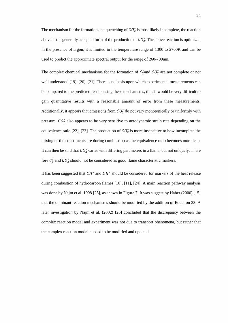
It has been suggested that 𝐶𝐶𝐻𝐻∗ and 𝐶𝐶𝐻𝐻∗ should be considered for markers of the heat release
during combustion of hydrocarbon flames [10], [11], [24]. A main reaction pathway analysis
was done by Najm et al. 1998 [25], as shown in Figure 7. It was suggest by Haber (2000) [15]
that the dominant reaction mechanisms should be modified by the addition of Equation 33. A
later investigation by Najm et al. (2002) [26] concluded that the discrepancy between the
complex reaction model and experiment was not due to transport phenomena, but rather that
the complex reaction model needed to be modified and updated.
25
Figure 7: Reaction Pathway Analysis of Premixed Methane-Air Combustion Showing the Formation of Chemiluminescent Species [25].
Extensive numerical and experimental studies have been performed on the production of 𝐶𝐶𝐻𝐻∗
and 𝐶𝐶𝐻𝐻∗ for variation in exhaust gas recirculation (EGR) [22], aerodynamic strain rate [13],
[22], pressure [13], [22], [27], preheat conditions [13], [22], percentage of complete combustion
[28], inlet axial Reynolds number [27] and equivalence ratio [13], [22], [27], [28].
26
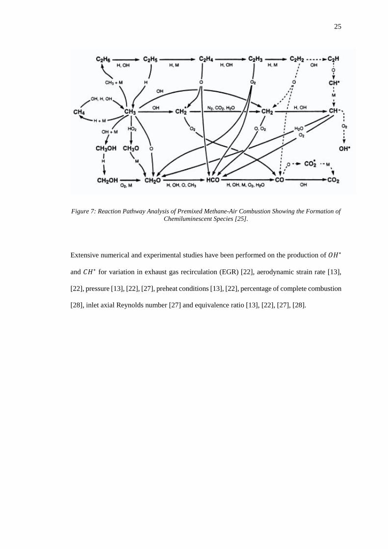
Equivalence Ratio
Figure 8: Numerical Prediction of the Production of OH* in Methane-Air Combustion at Various Pressures and Preheat Conditions [22].
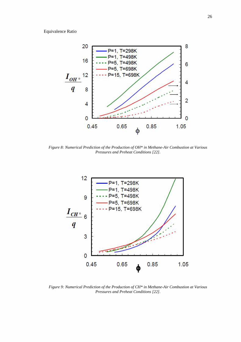
Figure 9: Numerical Prediction of the Production of CH* in Methane-Air Combustion at Various Pressures and Preheat Conditions [22].
27
Figure 10: Numerical Prediction of the Production of 𝐶𝐶𝐶𝐶2∗ in Methane-Air Combustion at Various Pressures and Preheat Conditions [22].
From Figure 9, Figure 10 and Figure 11 it is clear that at lean conditions the production of 𝐶𝐶𝐻𝐻∗,
𝐶𝐶𝐻𝐻∗ and 𝐶𝐶𝐶𝐶2∗ vary monotonically with equivalence ratio. Calibrating the data for each unique
system setup could allow for the variation of the chemiluminescent emissions to be used to
predict the local equivalence ratio.

28
EGR
Figure 11: Numerical Prediction of Product Recirculation Dependence of OH* (solid lines) and CH* (lines with symbols) in lean (𝜙𝜙=0.7) methane-air flames [22].
From Figure 11 it is clear that 𝐶𝐶𝐻𝐻∗ is insensitive to product recirculation at lean conditions, but
𝐶𝐶𝐻𝐻∗ increases more rapidly than the measured heat release for an increase in EGR. Pressure
and preheat conditions do not affect the sensitivity of 𝐶𝐶𝐻𝐻∗ and 𝐶𝐶𝐻𝐻∗ production to EGR.
Aerodynamic Strain Rate
The aerodynamic strain rate is a measure of the rate at which the flame stretches during
combustion. This effect affects the transport properties of the hot products and the flow of
reactants into the main reaction zone. The strain rate also can be a form of measurement of the
flame reactive wave acceleration.

29
Figure 12: Numerical Prediction of Strain Rate Dependence of OH* (solid lines) and CH* (lines with symbols) in lean (ϕ=0.7) methane-air flames [22].
From Figure 12, at low pressure conditions 𝐶𝐶𝐻𝐻∗ appears fairly sensitive to strain rate, but at
higher pressure 𝐶𝐶𝐻𝐻∗ becomes insensitive to strain rate. Similarly, 𝐶𝐶𝐻𝐻∗ is insensitive to strain
rate at elevated pressures. The work done by Ayoola et al. (2006) [29] in turbulent premixed
methane flames found that the spatially distributed 𝐶𝐶𝐻𝐻∗ chemiluminescent signal was skewed
correlated by the strain rate of the flame. This does not necessarily disagree with the predictions
made by Nori and Seitzman (2009) because the experiments were done at atmospheric pressure
and 𝐶𝐶𝐻𝐻∗ may vary wildly near lean blowout conditions.
2.5.2 Chemiluminescent Species as Possible Quantifiable Markers of Flame Properties
𝐶𝐶𝐻𝐻∗ appears to be the prime candidate for heat release due its formation off of the CH radical,
which is part of the dominant reaction in forming the products, however it is worrying that the
reaction R219, from Appendix A, has the ability to form 𝐶𝐶𝐻𝐻∗ at slightly lower temperatures.
This suggests that a bulk of the chemiluminescence emissions could come from the formation
𝐶𝐶𝐻𝐻∗ outside of the main reaction zone, depending on the local pressure and transport properties
30
of the flame. Other issue with 𝐶𝐶𝐻𝐻∗ chemiluminescence is the lifetime of the ground state
radical, which makes it prone to optical self-absorption.
It has been suggested that to mark where the heat release is occurring spatially that the 𝐶𝐶𝐻𝐻∗ to
𝐶𝐶𝐻𝐻∗ signal ratio be used. The 𝐶𝐶𝐻𝐻∗ radical is affected by the aerodynamic shear of turbulent
flames, which may skew any data collected. Taking the ratio between the two local emissions
signals could provide a measure of where both species are equivalently maximum, thus pointing
out spatially where the reaction zone might be. The production of OH* and CH* strongly
depends on the levels of the preceding radicals, which is dependent on the local mixture ratio
and the rate at which they are produced. An increase in local mixture ratio will result in a faster
relative increase in CH* production than OH*, with respect to equivalence ratio [30]. The rate
of dynamic change in the signal ratio could provide some information on the heat release rate
or the dynamics of the change in heat release rate locally.
Figure 13: Numerical Prediction of Equivalence Ratio in Methane-air Flames Using the Ratio of CH* and OH* Chemiluminescence [22].
31
Figure 14: Experimental Results of Equivalence Ratio in Methane-air Flames Using the Ratio of CH* and OH* Chemiluminescence for a Fixed Mass Flowrate of Preheated Air [27].
Comparing Figure 13 and Figure 14 it is clear that the numerical predictions fail to capture the
characteristic variation in the ratio between the chemiluminescent signals with respect to
equivalence ratio at elevated pressures. It is still unclear which physical mechanism is
responsible for this discrepancy between the data. At elevated pressures a number of physical
mechanisms or a combination of them could be responsible for discrepancies in the
experimental measurements with numerical predictions. One concern with line of sight
integrated measurements of chemiluminescent signals is the phenomenon of optical absorption
and scattering.
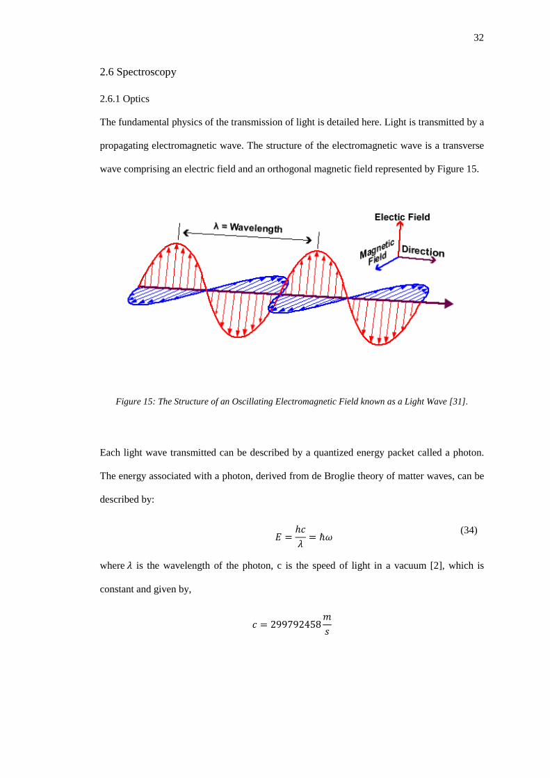
32
2.6 Spectroscopy
2.6.1 Optics
The fundamental physics of the transmission of light is detailed here. Light is transmitted by a
propagating electromagnetic wave. The structure of the electromagnetic wave is a transverse
wave comprising an electric field and an orthogonal magnetic field represented by Figure 15.
Figure 15: The Structure of an Oscillating Electromagnetic Field known as a Light Wave [31].
Each light wave transmitted can be described by a quantized energy packet called a photon.
The energy associated with a photon, derived from de Broglie theory of matter waves, can be
described by:
𝐸𝐸 =
ℎ𝑔𝑔𝜆𝜆
= ℏ𝜔𝜔 (34)
where 𝜆𝜆 is the wavelength of the photon, c is the speed of light in a vacuum [2], which is
constant and given by,
𝑔𝑔 = 299792458𝑔𝑔𝑠𝑠
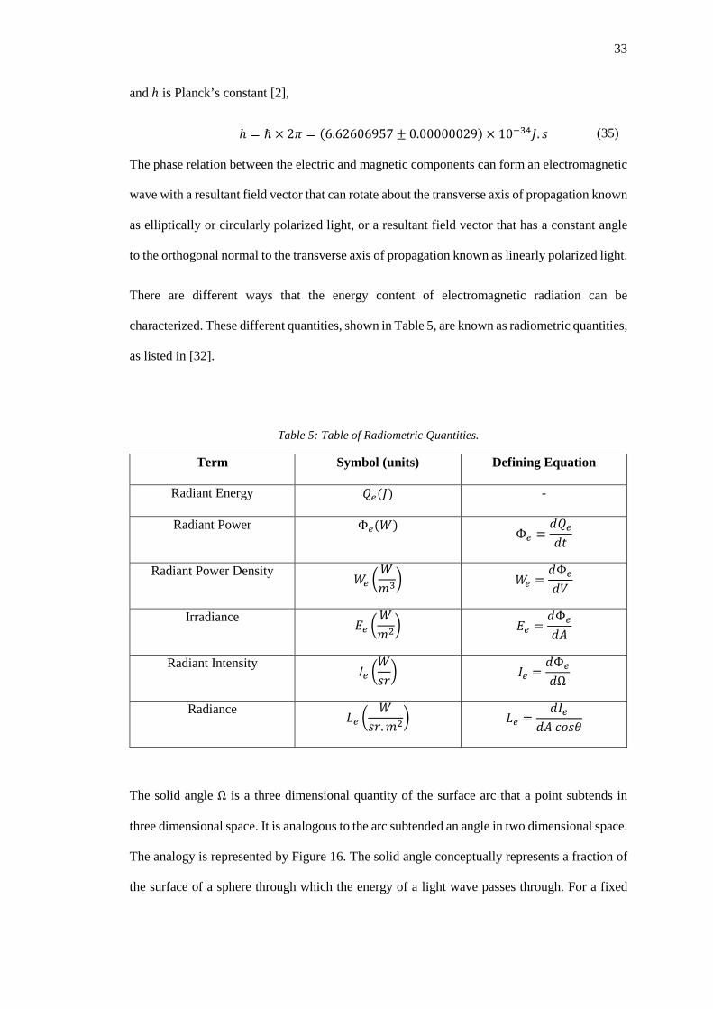
33
and ℎ is Planck’s constant [2],
ℎ = ℏ × 2𝜋𝜋 = (6.62606957 ± 0.00000029) × 10−34𝐽𝐽. 𝑠𝑠 (35)
The phase relation between the electric and magnetic components can form an electromagnetic
wave with a resultant field vector that can rotate about the transverse axis of propagation known
as elliptically or circularly polarized light, or a resultant field vector that has a constant angle
to the orthogonal normal to the transverse axis of propagation known as linearly polarized light.
There are different ways that the energy content of electromagnetic radiation can be
characterized. These different quantities, shown in Table 5, are known as radiometric quantities,
as listed in [32].
Table 5: Table of Radiometric Quantities.
Term Symbol (units) Defining Equation
Radiant Energy 𝑄𝑄𝑒𝑒(𝐽𝐽) -
Radiant Power Φ𝑒𝑒(𝑊𝑊) Φ𝑒𝑒 =𝑑𝑑𝑄𝑄𝑒𝑒𝑑𝑑𝑡𝑡
Radiant Power Density 𝑊𝑊𝑒𝑒 �𝑊𝑊𝑔𝑔3� 𝑊𝑊𝑒𝑒 =
𝑑𝑑Φ𝑒𝑒
𝑑𝑑𝑃𝑃
Irradiance 𝐸𝐸𝑒𝑒 �𝑊𝑊𝑔𝑔2� 𝐸𝐸𝑒𝑒 =
𝑑𝑑Φ𝑒𝑒
𝑑𝑑𝐴𝐴
Radiant Intensity 𝐼𝐼𝑒𝑒 �𝑊𝑊𝑠𝑠𝑏𝑏� 𝐼𝐼𝑒𝑒 =
𝑑𝑑Φ𝑒𝑒
𝑑𝑑Ω
Radiance 𝐿𝐿𝑒𝑒 �𝑊𝑊
𝑠𝑠𝑏𝑏.𝑔𝑔2� 𝐿𝐿𝑒𝑒 =𝑑𝑑𝐼𝐼𝑒𝑒
𝑑𝑑𝐴𝐴 𝑔𝑔𝑔𝑔𝑠𝑠𝑐𝑐
The solid angle Ω is a three dimensional quantity of the surface arc that a point subtends in
three dimensional space. It is analogous to the arc subtended an angle in two dimensional space.
The analogy is represented by Figure 16. The solid angle conceptually represents a fraction of
the surface of a sphere through which the energy of a light wave passes through. For a fixed
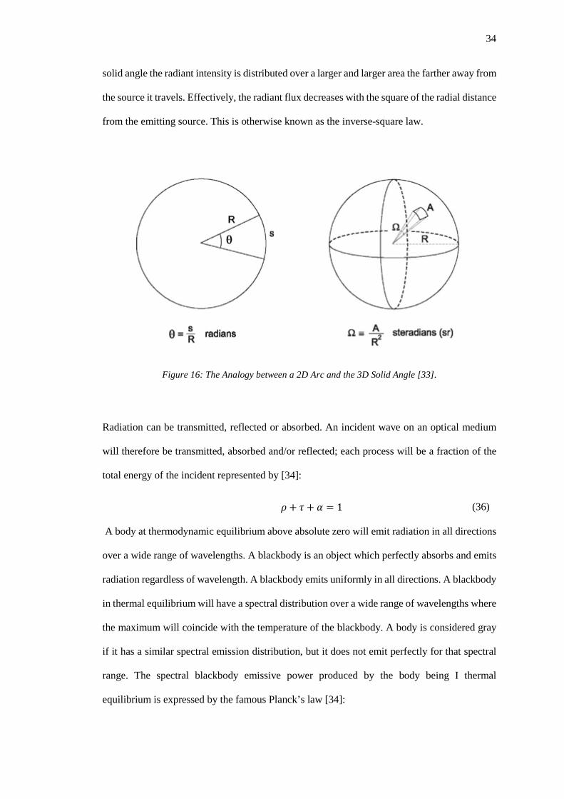
34
solid angle the radiant intensity is distributed over a larger and larger area the farther away from
the source it travels. Effectively, the radiant flux decreases with the square of the radial distance
from the emitting source. This is otherwise known as the inverse-square law.
Figure 16: The Analogy between a 2D Arc and the 3D Solid Angle [33].
Radiation can be transmitted, reflected or absorbed. An incident wave on an optical medium
will therefore be transmitted, absorbed and/or reflected; each process will be a fraction of the
total energy of the incident represented by [34]:
𝜌𝜌 + 𝜏𝜏 + 𝛼𝛼 = 1 (36)
A body at thermodynamic equilibrium above absolute zero will emit radiation in all directions
over a wide range of wavelengths. A blackbody is an object which perfectly absorbs and emits
radiation regardless of wavelength. A blackbody emits uniformly in all directions. A blackbody
in thermal equilibrium will have a spectral distribution over a wide range of wavelengths where
the maximum will coincide with the temperature of the blackbody. A body is considered gray
if it has a similar spectral emission distribution, but it does not emit perfectly for that spectral
range. The spectral blackbody emissive power produced by the body being I thermal
equilibrium is expressed by the famous Planck’s law [34]:

35
𝐿𝐿𝑒𝑒,𝑏𝑏𝑏𝑏(𝜆𝜆,𝑇𝑇) =
2𝜋𝜋ℎ𝑔𝑔2
𝜆𝜆5 �exp � ℎ𝑔𝑔𝜆𝜆𝑘𝑘𝐵𝐵𝑇𝑇
� − 1�
(37)
The wavelength at which the peak of the continuous distribution occurs at a specified
temperature is given by Wien’s displacement law as:
(𝜆𝜆𝑇𝑇)max 𝑝𝑝𝑡𝑡𝑝𝑝𝑒𝑒𝑟𝑟 = 2897.8 𝜇𝜇𝑔𝑔.𝐾𝐾 (38)
To understand how radiation propagates through an optical medium the fundamental equations
governing how electromagnetic fields interact with a dielectric must be used. The fundamental
equations which describe electromagnetic fields are collectively called the Maxwell’s
equations:
∇ ∙ 𝑬𝑬 =−∇ ∙ 𝑷𝑷𝜖𝜖0
(39)
∇ × 𝑬𝑬 = −
𝜕𝜕𝑩𝑩𝜕𝜕𝑡𝑡
(40)
∇ ∙ 𝑩𝑩 = 0 (41)
𝑔𝑔2∇× 𝑩𝑩 =
𝜕𝜕𝑬𝑬𝜕𝜕𝑡𝑡
+1𝜖𝜖0𝜕𝜕𝑷𝑷𝜕𝜕𝑡𝑡
(42)
The permittivity of free space is given by [2]:
𝜖𝜖0 = 8.854187817 … × 10−12𝐹𝐹𝑔𝑔
An incident electromagnetic wave on an atom or molecule can induce a dipole moment in the
atom or molecule; the dipole moment is a result of the electromagnetic field displacing the
electron cloud in such a way that there is a resulting electric field between the nucleus and the
excess electron portion of the asymmetric electron cloud. An illustration of an induced dipole
moment is shown in Figure 17.

36
Figure 17: Polarization Induced in a Molecule in the Presence of an Externally Applied Electric Field [35].
The polarization density 𝑷𝑷 is the vector quantity representing the density of permanent or
induced electric dipole moments in a dielectric substance. An incident electromagnetic wave
with frequency 𝜔𝜔 that is on or near an atomic transition applied to a collection of real electric-
dipole atoms that make up a homogeneous linear and isotropic dielectric medium will induce a
steady state vector polarization [36]:
𝑷𝑷(𝜔𝜔) = 𝝌𝝌(𝜔𝜔)𝜖𝜖0𝑬𝑬(𝜔𝜔) (43)
If the polarization is not linearly proportional to the electric field then the polarization can be
expressed as a higher order Taylor series expansion:
𝑃𝑃𝑖𝑖 = 𝜖𝜖0 ��𝜒𝜒𝑖𝑖𝑖𝑖
(1)𝐸𝐸𝑖𝑖𝑖𝑖
+ �𝜒𝜒𝑖𝑖𝑖𝑖𝑖𝑖(2)𝐸𝐸𝑖𝑖
𝑖𝑖𝑖𝑖
𝐸𝐸𝑖𝑖 + �𝜒𝜒𝑖𝑖𝑖𝑖𝑖𝑖𝑏𝑏(3) 𝐸𝐸𝑖𝑖
𝑖𝑖𝑖𝑖𝑏𝑏
𝐸𝐸𝑖𝑖𝐸𝐸𝑏𝑏 + ⋯� (44)

37
The dielectric medium’s susceptibility to polarization due to an electric field is represented
by 𝜒𝜒. For an atom or molecule within a gas that is randomly oriented the higher order effects
of susceptibility can be ignored. A classical approach to model a particles response to an
externally applied electric field can be utilized; this approach is called the classical electron
oscillator (CEO) model. The response of the electron cloud to an externally applied oscillating
electric field can modelled as a spring-mass-damper system analogous to a mechanical vibrator.
The differential function of the response can be expressed as [37]:
𝑑𝑑2𝜇𝜇𝑚𝑚(𝑡𝑡)𝑑𝑑𝑡𝑡2
+ 𝛾𝛾𝑑𝑑𝜇𝜇𝑚𝑚(𝑡𝑡)𝑑𝑑𝑡𝑡
+ 𝜔𝜔𝑎𝑎2𝜇𝜇𝑚𝑚(𝑡𝑡) = �𝑞𝑞2
𝑔𝑔𝑒𝑒�𝐸𝐸𝑚𝑚(𝑡𝑡)
(45)
𝑞𝑞 = (1.602176565 ± 0.000000035) × 10−19𝐶𝐶
𝑔𝑔𝑒𝑒 = (9.10938291 ± 0.00000040) × 10−31𝑘𝑘𝑔𝑔
The dipole moment for a single oscillator is defined as:
𝜇𝜇𝑚𝑚(𝑡𝑡) = 𝑞𝑞𝑥𝑥(𝑡𝑡) (46)
Where 𝑞𝑞 [2] is the elementary charge, 𝑥𝑥(𝑡𝑡) is the displacement response of an electron to an
externally applied electric field, 𝐸𝐸𝑚𝑚(𝑡𝑡) is the externally applied electric field, 𝑔𝑔𝑒𝑒 [2] is the
electron rest mass and 𝛾𝛾 is the spontaneous radiative emission rate, which damps the motion of
the CEO. Assuming that the incident electromagnetic wave induces a polarization at the same
frequency 𝜔𝜔, and expressing the incident electric field and the polarization as the average of
the wave and its complex conjugate, the resonant susceptibility of the CEO, after some
manipulation, can then be defined as [37]:
𝜒𝜒𝑟𝑟𝑒𝑒𝑟𝑟(𝜔𝜔) =𝑃𝑃0𝑚𝑚𝜖𝜖0𝐸𝐸0𝑚𝑚
= −𝑖𝑖𝑁𝑁𝑞𝑞2
𝜖𝜖0𝑔𝑔𝑒𝑒𝜔𝜔𝑎𝑎Δ𝜔𝜔𝑎𝑎�
1
�2𝑖𝑖(𝜔𝜔 − 𝜔𝜔𝑎𝑎)Δ𝜔𝜔𝑎𝑎
�+ 1�
(47)
The susceptibility for real atomic or molecular transitions can then be inferred by first collecting
the factors equivalent to the CEO radiative decay rate 𝛾𝛾, substituting and then replacing the
CEO radiative decay rate with the actual decay rate 𝐴𝐴12, the actual transition frequencies

38
calculated from energy transition levels and the rewriting of Equation (47 into real and
imaginary components to describe key processes during interaction:
𝜒𝜒𝑟𝑟𝑒𝑒𝑟𝑟(𝜔𝜔) = 𝜒𝜒′(𝜔𝜔) + 𝑖𝑖𝜒𝜒"(𝜔𝜔) = −𝑖𝑖𝜒𝜒0" �Δ𝑥𝑥
1 + (Δ𝑥𝑥)2 + 𝑖𝑖1
1 + (Δ𝑥𝑥)2� (48)
where,
𝜒𝜒0" =3(𝑛𝑛1 − 𝑛𝑛2)𝜆𝜆𝑎𝑎3𝐴𝐴12
4π2Δ𝜔𝜔𝑎𝑎
Describes strength of coupling between
transition and optic EM field.
Δ𝑥𝑥 = 2𝜔𝜔 − 𝜔𝜔𝑎𝑎Δ𝜔𝜔𝑎𝑎
Describes broadening of resonance
transition due to collisional and radiative
“damping”.
The effects of broadening on the transition emissions will be discussed at a later stage.
Analysis of electromagnetic radiation on a larger scale often involves a geometric approach.
For distance scales on an order much larger than the wavelength of the radiation this approach
is an adequate assumption to make. The geometric analysis always involves the investigation
of light passing through more than one type of medium; the “bend” in the incident light at the
interface between two optical media is of greatest concern in this approach.
The “bending” in the path of a light ray is due to reflection or refraction and is directly linked
to the concept of radiation propagation given by Equation 36. The behaviour of the light ray at
the interface is quantified by the optical property of refractive index. Geometrically the light
ray behaves according to Snell’s law [32], where incident angle with the interface normal
determines how much the ray would refract or even reflect. The relation between the incident
angle and the refraction angle is given by:
𝑠𝑠𝑖𝑖𝑛𝑛𝑐𝑐1𝑠𝑠𝑖𝑖𝑛𝑛𝑐𝑐2
=𝑣𝑣1𝑣𝑣2
=𝑛𝑛2𝑛𝑛1
(49)
39
The incident angle, velocity and refractive index are given by 𝑐𝑐1, 𝑣𝑣1 and 𝑛𝑛1 respectively, while
the refractive angle, exit velocity and exit medium refractive index are given by 𝑐𝑐2, 𝑣𝑣2 and 𝑛𝑛2
respectively. For gaseous media and visible light the refractive index is quite predictable and
linear because the resonant susceptibility frequency for most stable gases usually occurs in the
deep ultra-violet and the permeability of the gas is close to that of vacuum permeability.
Additionally, the refractive index increases slowly with frequency; this is known as normal
dispersion. Because the incident light ray with frequency 𝜔𝜔 will have an effect on the optical
medium it is propagating through, there is a relation between the resonant susceptibility, written
in a different form, of frequency 𝜔𝜔0 and the refractive index [35]:
𝜒𝜒 = 𝑛𝑛2 − 1 =
𝑁𝑁𝑞𝑞2
𝜖𝜖0𝑔𝑔𝑒𝑒(𝜔𝜔02 − 𝜔𝜔2 + 𝑖𝑖𝜔𝜔𝛾𝛾)
(50)
There are a multiplicity of natural frequencies in reality, so Equation 50 can be generalised as:
𝜒𝜒 = 𝑛𝑛2 − 1 =
𝑁𝑁𝑞𝑞2
𝜖𝜖0𝑔𝑔𝑒𝑒 �
𝑓𝑓𝑖𝑖(𝜔𝜔0,𝑖𝑖
2 − 𝜔𝜔2 + 𝑖𝑖𝜔𝜔𝛾𝛾𝑖𝑖)𝑖𝑖
(51)
, where 𝑓𝑓𝑖𝑖 is the fraction of the 𝑁𝑁 oscillators per unit volume having frequency 𝜔𝜔0,𝑖𝑖. Therefore
from Equation 51 light waves that have frequencies approaching that of the UV spectrum the
refractive index increase more rapidly with frequency.
2.6.2 Structure of Internal Energy Modes of Molecules
As a corollary of the photoelectric effect energy can be transferred to and from an atom or
molecule through a quantized energy packet of electromagnetic radiation called a photon. The
change in internal energy of the atom or molecule will correspond directly to the energy of the
incident or ejected photon from the atom or molecule. The number of photons that can be
absorbed by a particular material of thickness t can expressed as,
�
𝑑𝑑𝐼𝐼(𝑥𝑥)𝐼𝐼(𝑥𝑥)
𝑡𝑡
0= −𝜎𝜎𝑃𝑃𝐸𝐸𝑁𝑁� 𝑑𝑑𝑥𝑥
𝑡𝑡
0
(52)

40
where I is the number photons, 𝜎𝜎𝑃𝑃𝐸𝐸 is the absorbing cross-sectional area and N is the number
density of absorbing particles. This process is illustrated in Equation 37 and can be solved to
give the following form:
𝐼𝐼(𝑡𝑡) = 𝐼𝐼(0)𝑒𝑒−𝜎𝜎𝑃𝑃𝑃𝑃𝑁𝑁𝑡𝑡 (53)
Figure 18: An Illustration of a Beam of Photons Passing through a Slab Conveying the Concept of Absorption Cross Section [38].
In an atom or molecule the internal energy modes, especially for the electronic energy modes,
have discrete levels shown in Figure 19. This can be explained by the de Broglie matter wave
theory and the time independent Schrodinger wave equation for a simple harmonic oscillator
[38]:
∇2𝜓𝜓 =2𝑔𝑔ℏ2
[𝑃𝑃(𝑥𝑥) − 𝐸𝐸]𝜓𝜓 (54)
The wave function is labeled 𝜓𝜓, 𝑔𝑔 is the rest mass of an electron, V(x) is the potential energy
as function of the distance from the internuclear axis and E is the total energy. Solutions to
Equation 37 occur only at discrete values of E. These solutions are the eigenvalues of Equation
37 and the associate wave functions are termed the eigenfunctions [35].
41
Figure 19: Discrete Structure of the Potential Energy Levels Corresponding to the Different Modes of Internal Energy Storage of a Molecule [38].
Now assuming 𝝍𝝍(𝒙𝒙�, 𝑡𝑡) = 𝜓𝜓(𝒙𝒙�)exp (−2𝜋𝜋𝑖𝑖𝜈𝜈𝑡𝑡), from the viewpoint of the particle:
∇2𝝍𝝍(𝒙𝒙�, 𝑡𝑡) =
1𝑣𝑣2𝜕𝜕2𝝍𝝍(𝒙𝒙�, 𝑡𝑡)
𝜕𝜕𝑡𝑡2
(55)
Since 𝑣𝑣 = 𝜈𝜈𝜆𝜆 = 𝜈𝜈ℎ𝑝𝑝
and the momentum p may be expressed classically as �2𝑔𝑔�𝐸𝐸� − 𝑃𝑃(�̅�𝑥)�,
substituting into Equation 40, Equation 39 is obtained. It is interesting to note that from the
nature of the potential energy wells, Figure 19, for a molecule there appears to be some
42
restrictions on which electronic transitions are possible; these are known as selection rules and
will be discussed later.
According to Heisenberg’s uncertainty principle the position and the velocity of a particle
cannot be measured simultaneously exactly; there will be an uncertainty with at least one of the
measurements. That is to say, with an uncertainty (standard deviation from the expected value)
in the position ∆�̅�𝑥 and an uncertainty in the momentum ∆�̅�𝑝, the product of which must always
be at least:
∆�̅�𝑥.∆�̅�𝑝 ≥ ℏ (56)
The expected values can be calculated from the relation for the probability density function
[38]:
𝑃𝑃𝑑𝑑 = � 𝝍𝝍∗𝝍𝝍
∞
−∞
𝑑𝑑𝑃𝑃 = 1 (57)
Where V denotes volume. Then the expected values for position and momentum may be written
[38] as:
𝑥𝑥𝑚𝑚���� = � 𝝍𝝍∗�̅�𝑥𝝍𝝍
∞
−∞
𝑑𝑑𝑃𝑃 (58)
𝑝𝑝𝑚𝑚���� = � 𝝍𝝍∗�̅�𝑝𝝍𝝍
∞
−∞
𝑑𝑑𝑃𝑃 (59)
For an oscillating electron the angular momentum is constant within an isolated system,
according to wave mechanics it has to take on a discrete value in the same way that energy
does. In the case of an electron the angular momentum 𝒍𝒍 can have values of �𝑔𝑔(𝑔𝑔 + 1)ℏ or
approximately 𝑔𝑔ℏ. The azimuthal quantum number 𝑔𝑔 gives the orbital angular momentum in
units of ℏ, and takes on integer values. Similarly the electron has an angular momentum of its
own, denoted by 𝒔𝒔, and called electron spin. The electron spin has a magnitude of
�𝑠𝑠(𝑠𝑠 + 1)ℏ = 𝑔𝑔𝑟𝑟ℏ, where 𝑠𝑠 is the quantum number that only takes only takes on the value

43
𝑠𝑠 = ± 12 [24]. The trace pattern of the electron angular momentum is illustrated in Figure 20; it
is clear that the constant component 𝒎𝒎𝑏𝑏 of the orbital angular momentum in theory has the
range, −|𝒍𝒍| ≤ 𝒎𝒎𝑏𝑏 ≤ |𝒍𝒍|. However, in quantum theory, only the discrete values 𝑔𝑔𝑏𝑏 ≤ |𝑔𝑔|, 𝑔𝑔 ∈ ℤ;
𝑔𝑔𝑏𝑏 is called the magnetic quantum number of the electron. The total angular momentum of the
electron 𝒋𝒋 is given by the vector sum of its orbital angular momentum and spin 𝒋𝒋 = 𝒍𝒍 + 𝒔𝒔. As
with the other angular momentum variables the resultant angular momentum vector can also be
space quantized, such that 𝑔𝑔𝑖𝑖 = 𝑔𝑔𝑏𝑏 + 𝑔𝑔𝑟𝑟 = 𝑔𝑔𝑏𝑏 ± 12. Additionally, depending on the structure
of the atomic or molecular nuclei an electron can orbit within set energy tiers, known as orbitals.
These orbitals can be quantized with the value 𝑛𝑛 which take on the values 1, 2, 3, 𝑒𝑒𝑡𝑡𝑔𝑔.
corresponding to the 𝑠𝑠,𝑝𝑝,𝑑𝑑, 𝑒𝑒𝑡𝑡𝑔𝑔. orbitals.
Figure 20: Space Quantization of the Electron Orbital Angular Momentum and Spin within an Atom in the Presence of an Externally Applied Magnetic Field [35].

44
The Pauli Exclusion Principle states that [24]: “In one and the same atom, no two electrons can
have the same set of quantum numbers 𝑛𝑛, 𝑔𝑔,𝑔𝑔𝑏𝑏 , and 𝑔𝑔𝑟𝑟.” From Figure 20 it is easy to see that
the magnetic quantum number 𝑔𝑔𝑏𝑏 can take on 2𝑔𝑔 + 1 modes of motion or eigenfunctions, for
the same energy. The phenomenon whereby energy can be stored, for a specific energy value,
in various different modes within an atom is called degeneracy. Thus the magnetic quantum
number has a 2𝑔𝑔 + 1-fold degeneracy.
For light atoms with multiple electron systems there is a coupling between angular momenta of
several electrons, some of which are so strong that states with different orbital angular
momenta, denoted by 𝑳𝑳 have different energies. Similarly the total electron spin momentum
vector is 𝑺𝑺. The coupling between the 𝑳𝑳 and 𝑺𝑺 angular momentum vectors is aptly called LS
coupling or Russell-Saunders coupling [35]. The total angular momentum vector is therefore
labelled 𝑱𝑱𝒕𝒕𝒕𝒕𝒕𝒕 . However the 𝑳𝑳 and 𝑺𝑺 vectors cannot be oriented arbitrarily and this puts a
restriction on the coupling mechanism to form 𝑱𝑱𝒕𝒕𝒕𝒕𝒕𝒕.
For molecules two more modes of energy storage are introduced; vibration and rotation
between the molecules. Therefore it is possible to have coupling between the angular momenta
of the rotation and vibration between the molecules and the angular momenta of the multi-
electron system of the molecule. The Born-Oppenheimer approximation corresponds to the
assumption that the variation of the electronic wave function with nuclear coordinates is small;
this allows us to decouple and separate the wave function for the three types of energy storage
[24].
Rotational Energy Storage
Considering a rigid rovibrator, quantum mechanically the wave equation can describe the
behaviour since there is no potential energy (V=0) associated with a rigid rotator and fixed
internuclear axis. The energy associate with rotation of the molecule is quantized with the
following relation [24],
45
𝐸𝐸𝑟𝑟 =
ℎ2𝑔𝑔𝐽𝐽(𝐽𝐽 + 1)8𝜋𝜋2𝑔𝑔𝐼𝐼
= ℎ𝑔𝑔𝐵𝐵𝐽𝐽(𝐽𝐽 + 1) (60)
where 𝐽𝐽 is the rotational quantum number, which should not be confused with 𝑱𝑱𝒕𝒕𝒕𝒕𝒕𝒕, and 𝐼𝐼 is the
mass moment of inertia of the molecule. A correction due to the variation in the mass moment
of inertia due to the fact that a molecule is not a rigid rotator is handled by the introduction of
the term 𝐷𝐷, the centrifugal distortion constant, such that:
𝐸𝐸𝑟𝑟 = ℎ𝑔𝑔[𝐵𝐵𝐽𝐽(𝐽𝐽 + 1) − 𝐷𝐷𝐽𝐽2(𝐽𝐽 + 1)2] (61)
Since 𝐷𝐷 is always much smaller than 𝐵𝐵 it is sometimes left out depending on the level of impact
it has on the energy and how accurate the study needs to be.
Vibrational Energy Storage
Modelling a diatomic molecule as an anharmonic oscillator results in allowable vibrational
energies, with the inclusion of higher order terms [35],
𝐸𝐸𝑣𝑣 = ℎ𝑔𝑔 �𝜔𝜔𝑒𝑒 �𝑣𝑣 +
12� − 𝜔𝜔𝑒𝑒𝑥𝑥𝑒𝑒 �𝑣𝑣 +
12�2
+ 𝜔𝜔𝑒𝑒𝑦𝑦𝑒𝑒 �𝑣𝑣 +12�3
+ ⋯� (62)
where 𝜔𝜔𝑒𝑒 = 𝜈𝜈𝑐𝑐 is expressed in 𝑔𝑔𝑔𝑔−1 and 𝜔𝜔𝑒𝑒𝑥𝑥𝑒𝑒 ,𝜔𝜔𝑒𝑒𝑦𝑦𝑒𝑒 ≪ 𝜔𝜔𝑒𝑒. Usually, the molecule vibrates and
rotates at the same time; therefore as it vibrates the mass moment of inertia changes. Thus, there
needs to be a correction to the rotational constants to account for this discrepancy:
𝐵𝐵𝑣𝑣 = 𝐵𝐵𝑒𝑒 − 𝛼𝛼𝑒𝑒 �𝑣𝑣 +12�
(63)
𝐷𝐷𝑣𝑣 = 𝐷𝐷𝑒𝑒 + 𝛽𝛽𝑒𝑒 �𝑣𝑣 +12�
(64)
Where the subscript 𝑒𝑒 refers to the equilibrium positions of the nuclei, 𝛼𝛼𝑒𝑒 is referred to as the
vibration-rotation interaction constant.
Electronic Energy Storage
Similar to the case with atoms, for electronic modelling for molecules the principal n and
azimuthal l quantum numbers are employed. A new quantum number is introduced to
distinguish between the states given by n and l, whose magnitude is given by 𝜆𝜆 = ‖𝑔𝑔𝑏𝑏‖ and

46
direction is along the internuclear axis. A representation of the space quantization of the
electronic orbital angular momentum of a molecule is shown below in Figure 21.
Figure 21: Space Quantization of the Electron Orbital Angular Momentum and Spin within a Molecule in the Presence of an Externally Applied Magnetic Field, 𝒍𝒍 [35].
Now, the total orbital angular momentum for a multi-electron system is represented by the
quantum number 𝚲𝚲, given by [35],
𝚲𝚲 = �𝝀𝝀𝒊𝒊𝑖𝑖
(65)
The values that the total angular momentum quantum number can take is 𝚲𝚲 = 0, 1, 2, 3, …, and
are termed Σ,Π,Δ,Φ, etc. All states other than Σ are doubly degenerate due to the two opposing
directions that 𝚲𝚲 can point in. The resultant spin angular momentum is the sum of the individual
electron spins:
47
𝑺𝑺 = �𝒔𝒔𝒊𝒊𝑖𝑖
(66)
The resultant spin determines the state multiplicity by 2𝑆𝑆 + 1. There are a number of scenarios
where the states can further be split, and such instances are denoted by the preceding and
succeeding superscripts on the upper case Greek symbol. A side note: the quantum number
given by upper case Greek symbols are always a projection of the various angular momentum
vectors on the internuclear axis.
There are a number of coupling mechanisms between the various angular momenta within a
molecule, the most common ones for diatomic molecules are the Hund’s case (a) and Hund’s
case (b). Figure 22 show the different coupling mechanisms, where 𝛀𝛀 is the coupling sum
between the resultant orbital angular momentum 𝚲𝚲 and the resultant spin angular momentum,
𝑺𝑺, projected on the internuclear axis 𝚺𝚺. In Hund’s case (a) the spin-orbit coupling 𝛀𝛀 and the
nuclear rotation is assumed to be weak. Thus the total angular momentum can be describe using:
Hund’s Case (a) 𝑱𝑱 = 𝛀𝛀 + 𝑹𝑹 (67)
For Hund’s case (b) the spin coupling to the orbital angular momentum (nuclear axis) is weak,
so the spin couples to the rotation axis of the molecule. This case applies most often to Σ states
and often to Π,Δ states of low atomic number [35]. Therefore the angular momentum apart
from the spin can be grouped together to form a new quantum number 𝑵𝑵:
𝑵𝑵 = 𝑹𝑹 + 𝚲𝚲 (68)
The total angular momentum can then be described by:
Hund’s Case (b) 𝑱𝑱 = 𝑵𝑵 + 𝑺𝑺 (69)
In addition to spin splitting there is also Λ-doubling splitting when Λ ≠ 0.
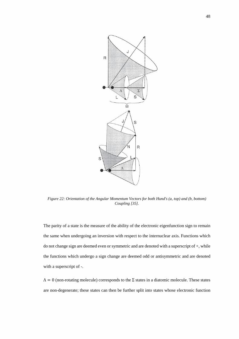
48
Figure 22: Orientation of the Angular Momentum Vectors for both Hund's (a, top) and (b, bottom) Coupling [35].
The parity of a state is the measure of the ability of the electronic eigenfunction sign to remain
the same when undergoing an inversion with respect to the internuclear axis. Functions which
do not change sign are deemed even or symmetric and are denoted with a superscript of +, while
the functions which undergo a sign change are deemed odd or antisymmetric and are denoted
with a superscript of -.
Λ = 0 (non-rotating molecule) corresponds to the Σ states in a diatomic molecule. These states
are non-degenerate; these states can then be further split into states whose electronic function

49
wave functions are symmetric or antisymmetric on reflection about any plane through the
internuclear axis. For the Σ+ states, the even J states will have a positive parity and the odd J
states will have a negative parity. For the Σ− states, the opposite is true.
In the case of homonuclear diatomic molecules there is also a centre symmetry at the midpoint
of the distance between the two nuclei. This means that when choosing the centre of symmetry
as the origin then the coordinates of all electrons are invariant with respect to the Hamiltonian
operation (quantum mechanical operator corresponding to the total energy of the system).
Therefore for a given value of Λ the different states can be classified according to their parity.
The orbital wave functions which are even under the inversion about the internuclear axis are
subscripted with g whereas the odd orbital wave functions gain a subscript u.
The selection rules for the transition between the various molecular states is shown in Table 6.
The transitions that are not allowed to happen according to the selection rules are called
forbidden transitions. These forbidden transitions are based on the theory of the coupling
mechanisms discussed here. There are theoretically an almost infinite number of ways that the
different states of momentum can couple, however some are extremely unlikely. Thus, on
occasion, some transitions that are deemed forbidden can happen, but often these transitions
have an extremely low probability and thus often do not produce significant emissions above
the noise levels of measurement.
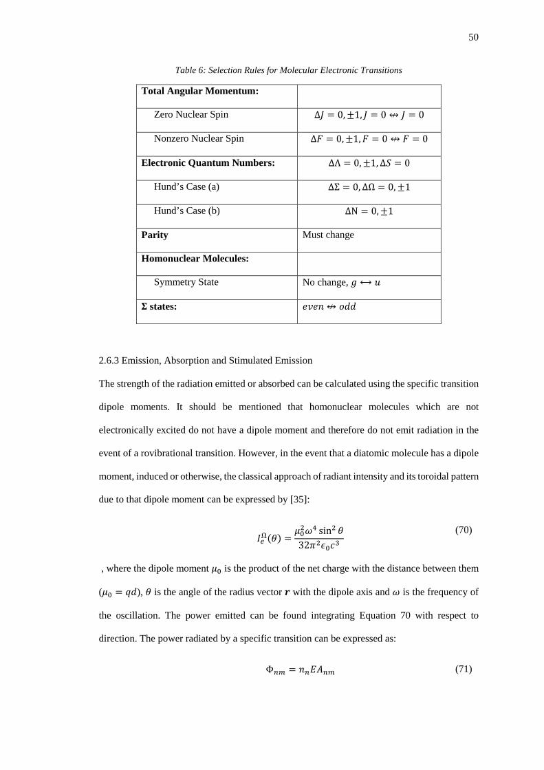
50
Table 6: Selection Rules for Molecular Electronic Transitions
Total Angular Momentum:
Zero Nuclear Spin Δ𝐽𝐽 = 0, ±1, 𝐽𝐽 = 0 ↮ 𝐽𝐽 = 0
Nonzero Nuclear Spin Δ𝐹𝐹 = 0, ±1,𝐹𝐹 = 0 ↮ 𝐹𝐹 = 0
Electronic Quantum Numbers: ΔΛ = 0, ±1,Δ𝑆𝑆 = 0
Hund’s Case (a) ΔΣ = 0,ΔΩ = 0, ±1
Hund’s Case (b) ΔN = 0, ±1
Parity Must change
Homonuclear Molecules:
Symmetry State No change, 𝑔𝑔 ⟷ 𝐹𝐹
𝚺𝚺 states: 𝑒𝑒𝑣𝑣𝑒𝑒𝑛𝑛 ↮ 𝑔𝑔𝑑𝑑𝑑𝑑
2.6.3 Emission, Absorption and Stimulated Emission
The strength of the radiation emitted or absorbed can be calculated using the specific transition
dipole moments. It should be mentioned that homonuclear molecules which are not
electronically excited do not have a dipole moment and therefore do not emit radiation in the
event of a rovibrational transition. However, in the event that a diatomic molecule has a dipole
moment, induced or otherwise, the classical approach of radiant intensity and its toroidal pattern
due to that dipole moment can be expressed by [35]:
𝐼𝐼𝑒𝑒Ω(𝑐𝑐) =
𝜇𝜇02𝜔𝜔4 sin2 𝑐𝑐32𝜋𝜋2𝜖𝜖0𝑔𝑔3
(70)
, where the dipole moment 𝜇𝜇0 is the product of the net charge with the distance between them
(𝜇𝜇0 = 𝑞𝑞𝑑𝑑), 𝑐𝑐 is the angle of the radius vector 𝒓𝒓 with the dipole axis and 𝜔𝜔 is the frequency of
the oscillation. The power emitted can be found integrating Equation 70 with respect to
direction. The power radiated by a specific transition can be expressed as:
Φ𝑛𝑛𝑚𝑚 = 𝑛𝑛𝑛𝑛𝐸𝐸𝐴𝐴𝑛𝑛𝑚𝑚 (71)

51
, where 𝑛𝑛𝑛𝑛 is the number of atoms or molecules in the upper energy state, 𝐸𝐸 is the energy of the
photon and 𝐴𝐴𝑛𝑛𝑚𝑚 is the Einstein coefficient of spontaneous emission. Combing Equations 70
and 71 a classical expression can be obtained for the coefficient of spontaneous emission. A
similar expression based on a quantum mechanical approach is given by [35]:
𝐴𝐴𝑛𝑛𝑚𝑚 =
2𝜔𝜔3
3ℎ𝑔𝑔3𝜖𝜖0𝑔𝑔𝑛𝑛|𝑅𝑅𝑛𝑛𝑚𝑚|2
(72)
, where 𝑔𝑔𝑛𝑛 is the degeneracy of the upper state and |𝑅𝑅𝑛𝑛𝑚𝑚|2 is the square of dipole matrix
element and is often referred to as the electronic transition probability. Equation 72 can be
expanded to include the matrix elements for the electronic, vibration and rotation transitions:
𝑅𝑅 = 𝑅𝑅𝑒𝑒𝑛𝑛𝑚𝑚𝑅𝑅𝑣𝑣𝑖𝑖𝑏𝑏𝑣𝑣′𝑣𝑣"𝑅𝑅𝑟𝑟𝑡𝑡𝑡𝑡𝐽𝐽′𝐽𝐽"
(73)
The electronic transition probability can be expressed using the probability density function of
the summation of the dipole moments for a multi-electron system derived from the Schrodinger
wave equation (Equation 57):
𝑅𝑅𝑒𝑒𝑛𝑛𝑚𝑚 = � 𝝍𝝍𝒎𝒎
∗ �𝜇𝜇𝝍𝝍𝒏𝒏
∞
−∞
𝑑𝑑𝑃𝑃 (74)
For molecules Equation 74 is notoriously difficult to calculate as there is a large number of
states along with the degeneracy at each of those states. In practice the transition probabilities
are found empirically. From basic quantum theory spontaneous emission should theoretically
not be able to occur. From quantum electrodynamics (QED) the electromagnetic field as a result
of the induced dipole moment must be quantized at every point in space; the electromagnetic
field has a ground state called the QED vacuum, which can mix with the excited stationary
states of the atom or molecule. The resulting interaction means that the stationary state is no
longer a true eigenstate of the combined system. The spontaneous emission in free space
depends on the vacuum fluctuations, which produce virtual particle-antiparticle pairs.
For the vibrational transition probabilities are called the Franck-Condon factors and are
expressed as:

52
𝑆𝑆𝑣𝑣′𝑣𝑣" = �𝑅𝑅𝑣𝑣𝑖𝑖𝑏𝑏𝑣𝑣
′𝑣𝑣"�2
= � � 𝝍𝝍𝒗𝒗′ 𝝍𝝍𝒗𝒗
"
∞
−∞
𝑑𝑑𝑃𝑃𝑛𝑛�
2
(75)
The Franck-Condon principle is a rule that explains the intensity of vibronic (vibrational-
electronic) transitions. It states that during an electronic transition, a change from one
vibrational energy level to another is most likely when the vibrational wave functions overlap
significantly. The assumption underlying the Franck-Condon principle is that the electronic
transition is so rapid that the nuclei are in the same location and have the same velocity after
the jump as before [35]. An image illustrating the Franck-Condon principle is shown below in
Figure 23.
Figure 23: Franck–Condon principle energy diagram. Since electronic transitions are very fast compared with nuclear motions, vibrational levels are favored when they correspond to a minimal
change in the nuclear coordinates. The potential wells are shown favouring v = 0 and v = 2.
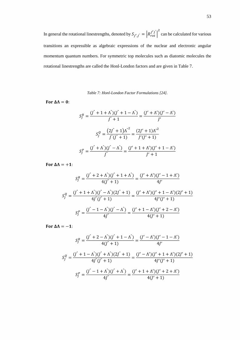
53
In general the rotational linestrengths, denoted by 𝑆𝑆𝐽𝐽′,𝐽𝐽" = �𝑅𝑅𝑟𝑟𝑡𝑡𝑡𝑡𝐽𝐽′𝐽𝐽"
�2 can be calculated for various
transitions an expressible as algebraic expressions of the nuclear and electronic angular
momentum quantum numbers. For symmetric top molecules such as diatomic molecules the
rotational linestrengths are called the Honl-London factors and are given in Table 7.
Table 7: Honl-London Factor Formulations [24].
𝐅𝐅𝐅𝐅𝐅𝐅 𝚫𝚫𝚲𝚲 = 𝟎𝟎:
𝑆𝑆𝐽𝐽𝑅𝑅 =(𝐽𝐽" + 1 + Λ")(𝐽𝐽" + 1 − Λ")
𝐽𝐽" + 1=
(𝐽𝐽′ + Λ′)(𝐽𝐽′ − Λ′)𝐽𝐽′
𝑆𝑆𝐽𝐽𝑄𝑄 =
�2𝐽𝐽" + 1�Λ"2
𝐽𝐽"(𝐽𝐽" + 1)=
(2𝐽𝐽′ + 1)Λ′2
𝐽𝐽′(𝐽𝐽′ + 1)
𝑆𝑆𝐽𝐽𝑃𝑃 =(𝐽𝐽" + Λ")(𝐽𝐽" − Λ")
𝐽𝐽" =(𝐽𝐽′ + 1 + Λ′)(𝐽𝐽′ + 1 − Λ′)
𝐽𝐽′ + 1
𝐅𝐅𝐅𝐅𝐅𝐅 𝚫𝚫𝚲𝚲 = +𝟏𝟏:
𝑆𝑆𝐽𝐽𝑅𝑅 =(𝐽𝐽" + 2 + Λ")(𝐽𝐽" + 1 + Λ")
4(𝐽𝐽" + 1)=
(𝐽𝐽′ + Λ′)(𝐽𝐽′ − 1 + Λ′)4𝐽𝐽′
𝑆𝑆𝐽𝐽𝑄𝑄 =
(𝐽𝐽" + 1 + Λ")(𝐽𝐽" − Λ")(2𝐽𝐽" + 1)4𝐽𝐽"(𝐽𝐽" + 1)
=(𝐽𝐽′ + Λ′)(𝐽𝐽′ + 1 − Λ′)(2𝐽𝐽′ + 1)
4𝐽𝐽′(𝐽𝐽′ + 1)
𝑆𝑆𝐽𝐽𝑃𝑃 =(𝐽𝐽" − 1 − Λ")(𝐽𝐽" − Λ")
4𝐽𝐽" =(𝐽𝐽′ + 1 − Λ′)(𝐽𝐽′ + 2 − Λ′)
4(𝐽𝐽′ + 1)
𝐅𝐅𝐅𝐅𝐅𝐅 𝚫𝚫𝚲𝚲 = −𝟏𝟏:
𝑆𝑆𝐽𝐽𝑅𝑅 =(𝐽𝐽" + 2 − Λ")(𝐽𝐽" + 1 − Λ")
4(𝐽𝐽" + 1)=
(𝐽𝐽′ − Λ′)(𝐽𝐽′ − 1 − Λ′)4𝐽𝐽′
𝑆𝑆𝐽𝐽𝑄𝑄 =
(𝐽𝐽" + 1 − Λ")(𝐽𝐽" + Λ")(2𝐽𝐽" + 1)4𝐽𝐽"(𝐽𝐽" + 1)
=(𝐽𝐽′ − Λ′)(𝐽𝐽′ + 1 + Λ′)(2𝐽𝐽′ + 1)
4𝐽𝐽′(𝐽𝐽′ + 1)
𝑆𝑆𝐽𝐽𝑃𝑃 =(𝐽𝐽" − 1 + Λ")(𝐽𝐽" + Λ")
4𝐽𝐽" =(𝐽𝐽′ + 1 + Λ′)(𝐽𝐽′ + 2 + Λ′)
4(𝐽𝐽′ + 1)

54
The resulting expression, combining Equation 72 with Equations 73, 74 and 75, for the Einstein
coefficient of spontaneous emission of a specific transition between the electronic, vibrational
and rotational levels is [35]:
𝐴𝐴𝑛𝑛𝑚𝑚,𝑣𝑣′𝑣𝑣",𝐽𝐽′𝐽𝐽" =
2𝜔𝜔3
3ℎ𝑔𝑔3𝜖𝜖0𝑔𝑔𝑛𝑛
|𝑅𝑅𝑒𝑒𝑛𝑛𝑚𝑚|2 �𝑅𝑅𝑣𝑣𝑖𝑖𝑏𝑏𝑣𝑣′𝑣𝑣"�2�𝑅𝑅𝑟𝑟𝑡𝑡𝑡𝑡
𝐽𝐽′𝐽𝐽"�2
2𝐽𝐽′ + 1
(76)
The inverse of Equation 76 describes the rate at which a particular transition happens, often
termed the transition decay rate:
𝜏𝜏𝑑𝑑𝑒𝑒𝑐𝑐𝑎𝑎𝑑𝑑 =1
𝐴𝐴𝑛𝑛𝑚𝑚,𝑣𝑣′𝑣𝑣",𝐽𝐽′𝐽𝐽"
(77)
In reality transitions are not monochromatic, they exhibit a breadth or width due to various
reasons. Broadening of the transition lines affects the spectral shape of the emission profile
emitted from an excited atom or molecule, and therefore impacts the interpretation of the
spectrum. For specific cases the line broadening can be used to determine pressure and
temperature.
There are two types of line broadening, namely homogeneous and inhomogeneous line
broadening. Homogeneous broadening is the result of dephasing of the signal due to collisions
and the statistical uncertainty involve with the Heisenberg uncertainty principle. Usually, the
effects of collisions on the broadening are much higher than the effect due to the uncertainty
principle; homogeneous broadening is usually referred to as collisional broadening.
The lineshapes follow a normalized distribution profile which satisfies
� 𝑔𝑔(𝜔𝜔,𝜔𝜔𝑎𝑎)+∞
−∞𝑑𝑑𝜔𝜔 = 1
(78)
The effect due homogeneous broadening can be expressed as the product of the line strength
and the normalized line profile. For absorption in particular this can be determined from the
absorbing part of the susceptibility found in Equation 48:

55
𝜒𝜒"(𝜔𝜔,𝜔𝜔𝑎𝑎) = 𝐾𝐾21𝑔𝑔𝐶𝐶(𝜔𝜔,𝜔𝜔𝑎𝑎) (79)
, where the line strength with the effects of degeneracy for each of the states is expressed as
[37]:
𝐾𝐾21 =�𝑔𝑔2𝑔𝑔1
𝑛𝑛1 − 𝑛𝑛2�𝜆𝜆212 𝐴𝐴214
(80)
, with 𝑔𝑔2 and 𝑔𝑔1 are the degeneracies of the upper and lower states respectively. The collisional
broadening profile can be written in normalized form, which takes a Lorentzian lineshape:
𝑔𝑔𝐶𝐶(𝜔𝜔,𝜔𝜔𝑎𝑎) =2𝜋𝜋Γ𝐶𝐶
11 + (Δ𝑥𝑥)2
(81)
, with:
Δ𝑥𝑥 = 2𝜔𝜔 − 𝜔𝜔𝑎𝑎Δ𝜔𝜔𝐻𝐻
The FWHM of the collisional broadening profile is given by Δ𝜔𝜔𝐻𝐻. Now, for a gas moving with
a velocity 𝑣𝑣𝑧𝑧 the resulting emissions radiated or absorbed by an ensemble of particles will cause
the radiation experienced by those particles to have a Doppler shift. Because the particles also
move in random directions the level of Doppler shift relative to the centreline frequency can be
described using a Maxwellian distribution function. The normalized distribution function,
which takes the form of a Gaussian curve, is
𝑔𝑔𝐷𝐷(𝜔𝜔𝑎𝑎) = �
4ln (2)𝜋𝜋(Δ𝜔𝜔𝐷𝐷)2 exp �−4 𝑔𝑔𝑛𝑛(2) �
𝜔𝜔𝑎𝑎 − 𝜔𝜔𝑎𝑎,0
𝛥𝛥𝜔𝜔𝐷𝐷�2�
(82)
, with the shift in centreline frequency as:
𝜔𝜔𝑎𝑎 = �1 +𝑣𝑣𝑧𝑧𝑔𝑔�𝜔𝜔𝑎𝑎,0

56
The Doppler linewidth at FWHM is:
𝛥𝛥𝜔𝜔𝐷𝐷 = 𝜔𝜔𝑎𝑎,0�
8 ln(2)𝑘𝑘𝐵𝐵𝑇𝑇𝑔𝑔𝑎𝑎𝑔𝑔2
(83)
, where 𝑔𝑔𝑎𝑎 is the mass of the molecule. Practically, both effects of line broadening occur at the
same time to a greater or lesser degree depending on the properties of the gas. To account for
both effects an approximation to the normalize line profile can be achieved by taking the
convolution of the collisional and Doppler line profiles. The convolution of the two profiles is
called the Voigt profile:
𝑔𝑔𝑉𝑉(𝜔𝜔,𝜔𝜔𝑎𝑎) = � 𝑔𝑔𝐷𝐷(𝜔𝜔𝑎𝑎)𝑔𝑔𝐶𝐶(𝜔𝜔 − 𝜔𝜔𝑎𝑎)𝑑𝑑𝜔𝜔
+∞
−∞
(84)
The resulting profile can be expressed as:
𝑔𝑔𝑉𝑉(𝜔𝜔,𝜔𝜔𝑎𝑎) = 2�
ln (2)𝜋𝜋
𝑃𝑃(𝑎𝑎, 𝑥𝑥)Δ𝜔𝜔𝐷𝐷
(85)
, where the Voigt profile 𝑃𝑃(𝑎𝑎, 𝑥𝑥) is given by:
𝑃𝑃(𝑎𝑎, 𝑥𝑥) =
𝑎𝑎𝜋𝜋�
exp (−𝑦𝑦2)𝑎𝑎2 + (𝑥𝑥 − 𝑦𝑦)2 𝑑𝑑𝑦𝑦
+∞
−∞
(86)
𝑎𝑎 and 𝑥𝑥 are defined as
𝑎𝑎 = �ln (2)Δ𝜔𝜔𝐶𝐶
Δ𝜔𝜔𝐷𝐷
𝑥𝑥 = 2�ln (2)(𝜔𝜔 − 𝜔𝜔𝑎𝑎)Δ𝜔𝜔𝐷𝐷
To date there is no known analytical solution for Equation 86, but there have been numerous
articles with regards to numerically computing the profile. Now that the normalized lineshapes
have been dealt with the effect of absorption on incident radiation can be calculated. The
expression can utilise any one of the radiometric quantities expressed in Table 5 because the
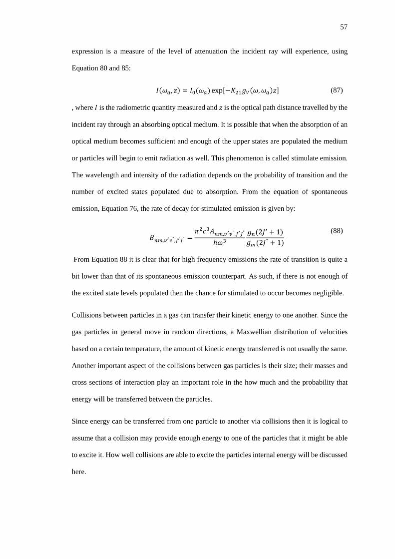
57
expression is a measure of the level of attenuation the incident ray will experience, using
Equation 80 and 85:
𝐼𝐼(𝜔𝜔𝑎𝑎, 𝑧𝑧) = 𝐼𝐼0(𝜔𝜔𝑎𝑎) exp[−𝐾𝐾21𝑔𝑔𝑉𝑉(𝜔𝜔,𝜔𝜔𝑎𝑎)𝑧𝑧] (87)
, where 𝐼𝐼 is the radiometric quantity measured and 𝑧𝑧 is the optical path distance travelled by the
incident ray through an absorbing optical medium. It is possible that when the absorption of an
optical medium becomes sufficient and enough of the upper states are populated the medium
or particles will begin to emit radiation as well. This phenomenon is called stimulate emission.
The wavelength and intensity of the radiation depends on the probability of transition and the
number of excited states populated due to absorption. From the equation of spontaneous
emission, Equation 76, the rate of decay for stimulated emission is given by:
𝐵𝐵𝑛𝑛𝑚𝑚,𝑣𝑣′𝑣𝑣",𝐽𝐽′𝐽𝐽" =
𝜋𝜋2𝑔𝑔3𝐴𝐴𝑛𝑛𝑚𝑚,𝑣𝑣′𝑣𝑣",𝐽𝐽′𝐽𝐽"
ℎ𝜔𝜔3𝑔𝑔𝑛𝑛(2𝐽𝐽′ + 1)𝑔𝑔𝑚𝑚(2𝐽𝐽" + 1)
(88)
From Equation 88 it is clear that for high frequency emissions the rate of transition is quite a
bit lower than that of its spontaneous emission counterpart. As such, if there is not enough of
the excited state levels populated then the chance for stimulated to occur becomes negligible.
Collisions between particles in a gas can transfer their kinetic energy to one another. Since the
gas particles in general move in random directions, a Maxwellian distribution of velocities
based on a certain temperature, the amount of kinetic energy transferred is not usually the same.
Another important aspect of the collisions between gas particles is their size; their masses and
cross sections of interaction play an important role in the how much and the probability that
energy will be transferred between the particles.
Since energy can be transferred from one particle to another via collisions then it is logical to
assume that a collision may provide enough energy to one of the particles that it might be able
to excite it. How well collisions are able to excite the particles internal energy will be discussed
here.

58
The probability and cross sections of the energy transfer process are usually proportional to the
adiabatic Massey parameter. If one is to consider a collision between an oscillator BC
(molecule) and a particle A the response of the oscillator to a perturbing external force can be
modelled as a spring-mass system [39]:
Figure 24: Spring-Mass System Analogy for a Collision between a Molecule and a Particle [39].
For an initially non-vibrating oscillator, the system will have the following equation an initial
conditions:
�̈�𝑦 + 𝜔𝜔2𝑦𝑦 =1𝑔𝑔𝐹𝐹(𝑡𝑡),𝑔𝑔 =
𝑔𝑔𝐵𝐵𝑔𝑔𝐶𝐶
𝑔𝑔𝐵𝐵 + 𝑔𝑔𝐶𝐶
𝑦𝑦(−∞) = 0, �̇�𝑦 = (−∞) = 0
(89)
, where 𝜔𝜔 is the resonant frequency of the system. Integrating, we obtain the energy transferred
to the oscillator:
Δ𝐸𝐸 =
12𝑔𝑔
�� 𝐹𝐹(𝑡𝑡)𝑒𝑒−𝑖𝑖𝑖𝑖𝑡𝑡𝑑𝑑𝑡𝑡∞
−∞�2
(90)
The transferred energy is therefore determine by the square of the resonant Fourier component
at the oscillator frequency of the perturbing force. Since the heavy particles (atoms and
molecules) have a much slower velocity than the electrons in those particles, even when they
have enough kinetic energy, they cannot transfer enough energy to those electrons inside the
particles because the process is far from resonance. This effect is a reflection of a general
principle of particle interaction. A slow motion is adiabatic; it is reluctant to transfer energy to
a fast motion. The adiabatic principle can be explained in terms of relations between low

59
interaction frequency 𝜔𝜔𝑖𝑖𝑛𝑛𝑡𝑡 = 𝛼𝛼𝑣𝑣 (reverse time of interaction between particles) and high
frequency of electron transfer in particle 𝜔𝜔𝑡𝑡𝑟𝑟 = Δ𝐸𝐸ℏ
. Here 1𝛼𝛼
is the characteristic size of the
interacting neutral particles; 𝑣𝑣 is their velocity; Δ𝐸𝐸 is the change in electron energy in a particle
(atom or molecule) during the interaction.
From Equation 90, only the fast Fourier components of the slow interaction potential between
the particles with frequencies about 𝜔𝜔𝑡𝑡𝑟𝑟 provide the energy transfer between the interacting
particles. The Massey exponent detailing the probability and cross sections of the energy
transfer process are given by [40]:
𝑃𝑃𝐸𝐸𝑛𝑛𝑇𝑇𝑟𝑟 ∝ exp �−𝜔𝜔𝑡𝑡𝑟𝑟
𝜔𝜔𝑖𝑖𝑛𝑛𝑡𝑡� ∝ exp �−
𝛥𝛥𝐸𝐸ℏ𝛼𝛼𝑣𝑣
� = exp(−𝑃𝑃𝑀𝑀𝑎𝑎) (91)
The adiabatic Massey parameter is given by 𝑃𝑃𝑀𝑀𝑎𝑎 = 𝛥𝛥𝐸𝐸ℏ𝛼𝛼𝑣𝑣
. If 𝑃𝑃𝑀𝑀𝑎𝑎 ≫ 1 then the process is
adiabatic and its probability is exponentially low. To get the Massey parameter close enough
to one for the process of electronic excitation of a molecule the energy of the molecule needs
to be on the order of 10keV and above. From a modified version for energy, Equation 4 shows
that 10keV corresponds to a temperature of 77.35 × 10⁶K! This energy is about three order of
magnitude larger than the ionization potential, thus excitation through the process of collision
by atoms and molecules is inefficient and extremely unlikely to happen.
With that being said, the process of energy transfer to and from the vibration states of a
molecule are quite easily excited. For some molecules the cross sections of interactions of
certain molecules of interest with various collision partners have been documented. The process
of energy transfer with respect to the vibration states can be done even when a molecule is in
an electronically excited state. The process where the collisions cause the electronically excited
state of a molecule to decay to a vibrationally excited, electronically passive state is sometimes
called collisional quenching of that molecule. If the temperatures of the collision partners are
high enough it is possible to put the electronically excite molecule into a higher vibrationally

60
excited state. The resulting decay from such an energy level results in a shorter wavelength
radiative emission than from the “normal” electronically excited state.
2.6.4 Spectra of Emissions
From statistical thermodynamics an ensemble of particles of a particular species at a certain
state or macrostate will have a distribution of microstates corresponding to the macrostate. The
distribution of possible energy microstates can attain by translation, rotation, vibration,
electronic excitation and nuclear states follow the Maxwell-Boltzmann distribution [3]:
𝑁𝑁𝑖𝑖 = 𝑁𝑁𝑔𝑔𝑖𝑖𝑒𝑒
−𝐸𝐸𝑗𝑗𝑖𝑖𝐵𝐵𝑇𝑇
∑ 𝑔𝑔𝑖𝑖𝑒𝑒−𝐸𝐸𝑗𝑗𝑖𝑖𝐵𝐵𝑇𝑇𝑖𝑖
(92)
, where 𝑁𝑁𝑖𝑖 is the number density of the particles in the 𝑗𝑗𝑡𝑡ℎ state of energy 𝐸𝐸𝑖𝑖; 𝑁𝑁 the total number
density and 𝑔𝑔𝑖𝑖 degeneracy of the state. The denominator of Equation 92 is termed the partition
function and is denoted by 𝑍𝑍. For an ideal diatomic gas the energy modes are uncoupled in the
Born-Oppenheimer approximation [37]:
𝐸𝐸𝑖𝑖,𝑖𝑖,𝑖𝑖,𝑏𝑏,𝑚𝑚 = (𝐸𝐸𝑖𝑖)𝑡𝑡𝑟𝑟 + �𝐸𝐸𝑖𝑖�𝑟𝑟𝑡𝑡𝑡𝑡 + (𝐸𝐸𝑖𝑖)𝑣𝑣𝑖𝑖𝑏𝑏 + (𝐸𝐸𝑏𝑏)𝑒𝑒𝑏𝑏𝑒𝑒𝑐𝑐 + (𝐸𝐸𝑚𝑚)𝑛𝑛𝑢𝑢𝑐𝑐 (93)
The indices (𝑖𝑖, 𝑗𝑗,𝑘𝑘, 𝑔𝑔,𝑔𝑔) refer to a particular energy level. The total degeneracy of a level is
then given by:
𝑔𝑔𝑖𝑖,𝑖𝑖,𝑖𝑖,𝑏𝑏,𝑚𝑚 = (𝑔𝑔𝑖𝑖)𝑡𝑡𝑟𝑟�𝑔𝑔𝑖𝑖�𝑟𝑟𝑡𝑡𝑡𝑡(𝑔𝑔𝑖𝑖)𝑣𝑣𝑖𝑖𝑏𝑏(𝑔𝑔𝑏𝑏)𝑒𝑒𝑏𝑏𝑒𝑒𝑐𝑐(𝑔𝑔𝑚𝑚)𝑛𝑛𝑢𝑢𝑐𝑐 (94)
The results from Equation 93 and 94 allow us to write the total partition function from Equation
92 as the product of the partition function for each energy mode:
𝑍𝑍 = 𝑍𝑍𝑡𝑡𝑟𝑟𝑍𝑍𝑟𝑟𝑡𝑡𝑡𝑡𝑍𝑍𝑣𝑣𝑖𝑖𝑏𝑏𝑍𝑍𝑒𝑒𝑏𝑏𝑒𝑒𝑐𝑐𝑍𝑍𝑛𝑛𝑢𝑢𝑐𝑐 (95)
The nuclear partition function is only of concern when considering homonuclear molecules
where the symmetry of the molecule affects the distribution of the rotational energy states. For
heteronuclear molecules the nuclear partition function can be neglected. The electronic partition
function is defined for each electronic level, but because most excited electronic levels have

61
temperatures on the order of 105K, usually no more than a couple of terms are required to
approximate the partition function accurately. The vibration partition function can be derived
to the form [37]:
𝑍𝑍𝑣𝑣𝑖𝑖𝑏𝑏 =
exp �−𝑐𝑐𝑣𝑣𝑖𝑖𝑏𝑏2𝑇𝑇 �
1 − exp �−𝑐𝑐𝑣𝑣𝑖𝑖𝑏𝑏𝑇𝑇 �
(96)
The vibrational temperature can be approximated, using Equation 62, as:
𝑐𝑐𝑣𝑣𝑖𝑖𝑏𝑏 = �
ℎ𝑔𝑔𝑘𝑘𝐵𝐵�𝜔𝜔𝑒𝑒
(97)
In a similar process the rotational distribution function for heteronuclear molecules can be
derived to the form:
𝑍𝑍𝑟𝑟𝑡𝑡𝑡𝑡 =𝑇𝑇𝑐𝑐𝑟𝑟𝑡𝑡𝑡𝑡
(98)
The rotational temperature can be approximated, using Equation 63, as:
𝑐𝑐𝑟𝑟𝑡𝑡𝑡𝑡 = �
ℎ𝑔𝑔𝑘𝑘𝐵𝐵�𝐵𝐵𝑒𝑒
(99)
From Equation 98 it is clear that as the temperature is increased the rotational temperature is
increased. This leads to an increase in the denominator of the overall distribution function
shifting the distribution in favour of the higher rotational states. This will cause the output of
the spectrum to be stronger toward the states associated with the higher rotational levels. From
this shift it is possible to infer from measurements of a hot gas the temperature of that gas, as
long as the spectrum is resolved adequately. The final form of the Maxwell-Boltzmann
distribution function can be expressed as:
𝑛𝑛1𝑛𝑛𝑔𝑔𝑟𝑟𝑡𝑡𝑢𝑢𝑛𝑛𝑑𝑑
=
𝑔𝑔1 exp �−� 𝜖𝜖ℎ𝑔𝑔� �
ℎ𝑔𝑔𝑘𝑘𝐵𝐵�
𝑇𝑇 �
𝑍𝑍𝑒𝑒𝑏𝑏𝑒𝑒𝑐𝑐𝑍𝑍𝑣𝑣𝑖𝑖𝑏𝑏𝑍𝑍𝑟𝑟𝑡𝑡𝑡𝑡
(100)
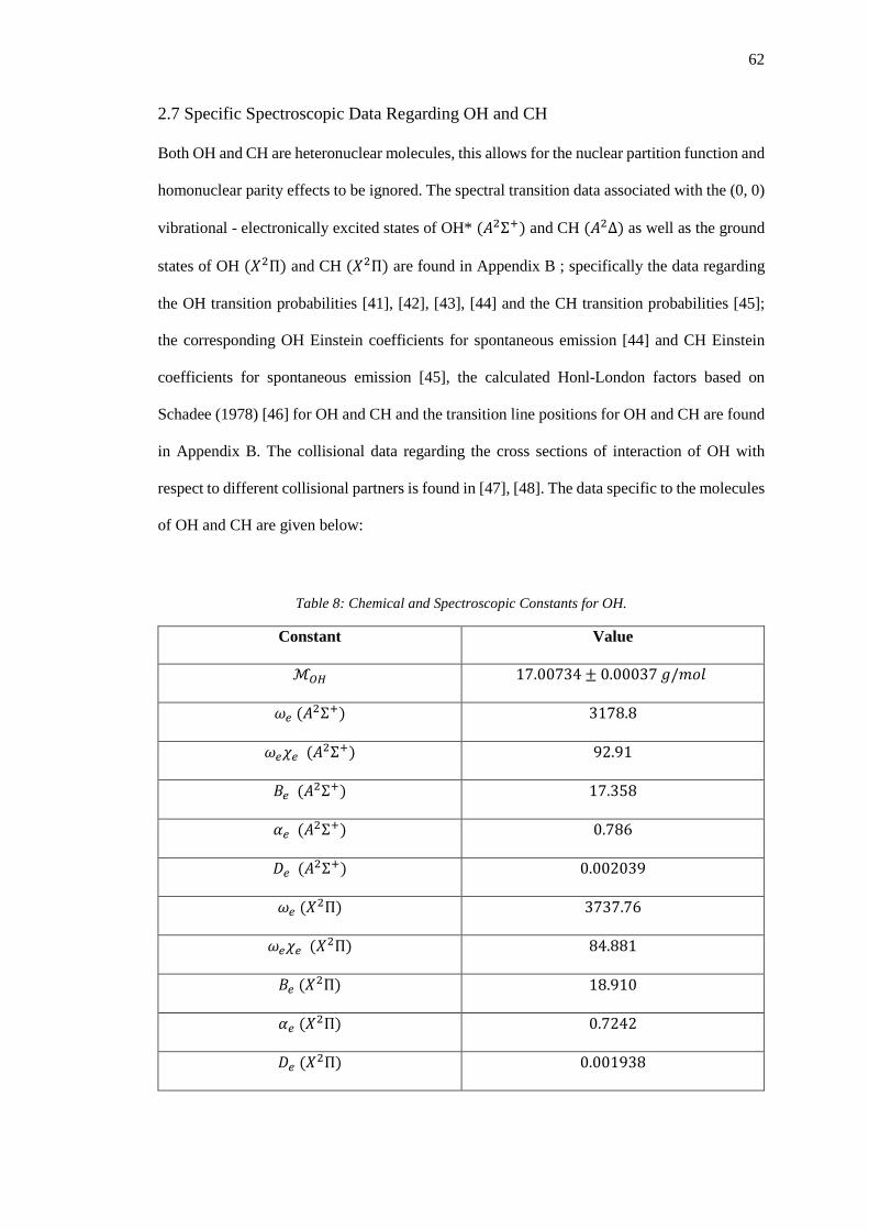
62
2.7 Specific Spectroscopic Data Regarding OH and CH
Both OH and CH are heteronuclear molecules, this allows for the nuclear partition function and
homonuclear parity effects to be ignored. The spectral transition data associated with the (0, 0)
vibrational - electronically excited states of OH* (𝐴𝐴2Σ+) and CH (𝐴𝐴2Δ) as well as the ground
states of OH (𝑋𝑋2Π) and CH (𝑋𝑋2Π) are found in Appendix B ; specifically the data regarding
the OH transition probabilities [41], [42], [43], [44] and the CH transition probabilities [45];
the corresponding OH Einstein coefficients for spontaneous emission [44] and CH Einstein
coefficients for spontaneous emission [45], the calculated Honl-London factors based on
Schadee (1978) [46] for OH and CH and the transition line positions for OH and CH are found
in Appendix B. The collisional data regarding the cross sections of interaction of OH with
respect to different collisional partners is found in [47], [48]. The data specific to the molecules
of OH and CH are given below:
Table 8: Chemical and Spectroscopic Constants for OH.
Constant Value
ℳ𝑂𝑂𝐻𝐻 17.00734 ± 0.00037 𝑔𝑔/𝑔𝑔𝑔𝑔𝑔𝑔
𝜔𝜔𝑒𝑒 (𝐴𝐴2Σ+) 3178.8
𝜔𝜔𝑒𝑒𝜒𝜒𝑒𝑒 (𝐴𝐴2Σ+) 92.91
𝐵𝐵𝑒𝑒 (𝐴𝐴2Σ+) 17.358
𝛼𝛼𝑒𝑒 (𝐴𝐴2Σ+) 0.786
𝐷𝐷𝑒𝑒 (𝐴𝐴2Σ+) 0.002039
𝜔𝜔𝑒𝑒 (𝑋𝑋2Π) 3737.76
𝜔𝜔𝑒𝑒𝜒𝜒𝑒𝑒 (𝑋𝑋2Π) 84.881
𝐵𝐵𝑒𝑒 (𝑋𝑋2Π) 18.910
𝛼𝛼𝑒𝑒 (𝑋𝑋2Π) 0.7242
𝐷𝐷𝑒𝑒 (𝑋𝑋2Π) 0.001938

63
Table 9: Chemical and Spectroscopic Constants for CH.
Constant Value
ℳ𝐶𝐶𝐻𝐻 13.01864 ± 0.00087 𝑔𝑔/𝑔𝑔𝑔𝑔𝑔𝑔
𝜔𝜔𝑒𝑒 (𝐴𝐴2Δ) 2950.7
𝜔𝜔𝑒𝑒𝜒𝜒𝑒𝑒 (𝐴𝐴2Δ) 96.65
𝐵𝐵𝑒𝑒 (𝐴𝐴2Δ) 14.934
𝛼𝛼𝑒𝑒 (𝐴𝐴2Δ) 0.697
𝐷𝐷𝑒𝑒 (𝐴𝐴2Δ) 0.00154
𝜔𝜔𝑒𝑒 (𝑋𝑋2Π) 2858.5
𝜔𝜔𝑒𝑒𝜒𝜒𝑒𝑒 (𝑋𝑋2Π) 63.02
𝐵𝐵𝑒𝑒 (𝑋𝑋2Π) 14.457
𝛼𝛼𝑒𝑒 (𝑋𝑋2Π) 0.534
𝐷𝐷𝑒𝑒 (𝑋𝑋2Π) 0.00145
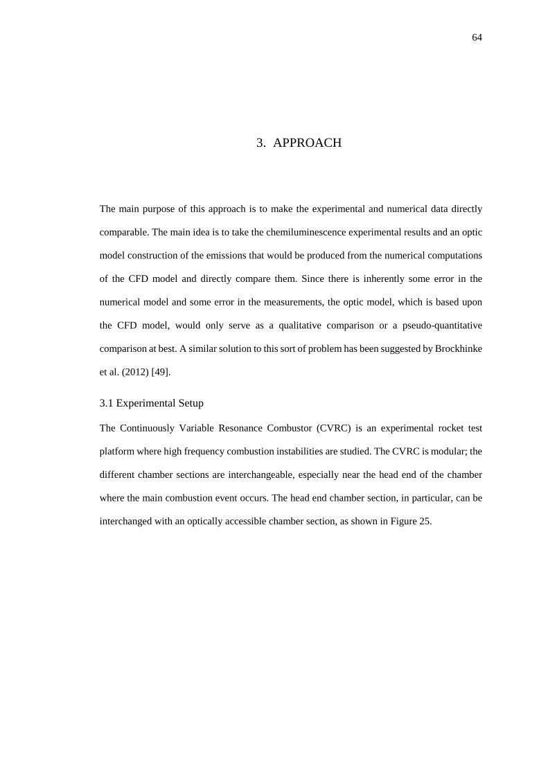
64
3. APPROACH
The main purpose of this approach is to make the experimental and numerical data directly
comparable. The main idea is to take the chemiluminescence experimental results and an optic
model construction of the emissions that would be produced from the numerical computations
of the CFD model and directly compare them. Since there is inherently some error in the
numerical model and some error in the measurements, the optic model, which is based upon
the CFD model, would only serve as a qualitative comparison or a pseudo-quantitative
comparison at best. A similar solution to this sort of problem has been suggested by Brockhinke
et al. (2012) [49].
3.1 Experimental Setup
The Continuously Variable Resonance Combustor (CVRC) is an experimental rocket test
platform where high frequency combustion instabilities are studied. The CVRC is modular; the
different chamber sections are interchangeable, especially near the head end of the chamber
where the main combustion event occurs. The head end chamber section, in particular, can be
interchanged with an optically accessible chamber section, as shown in Figure 25.
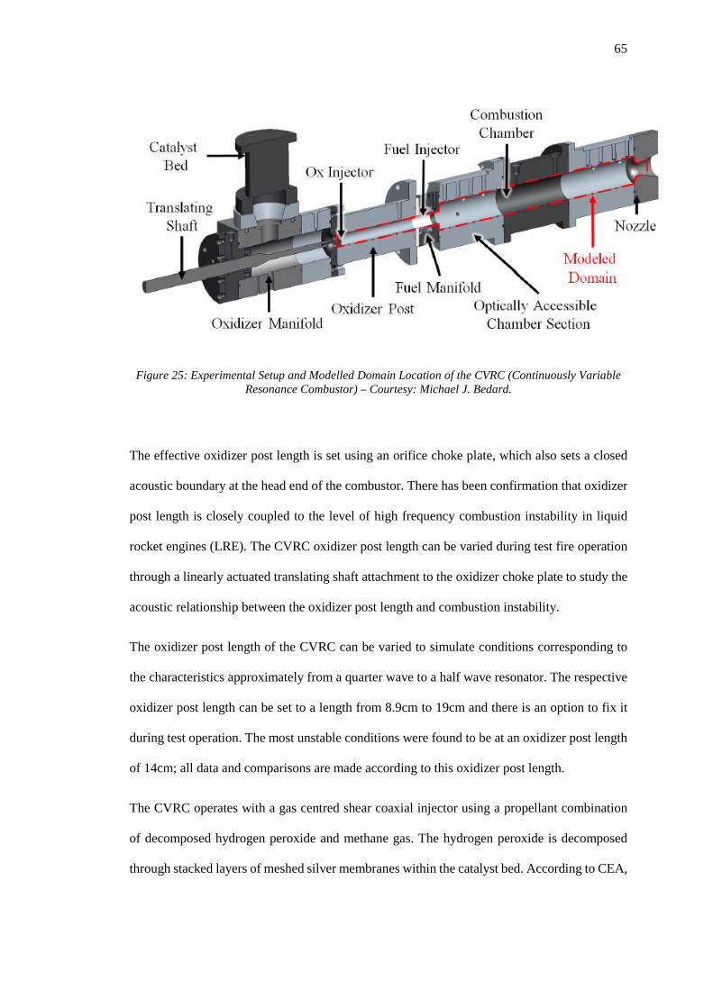
65
Figure 25: Experimental Setup and Modelled Domain Location of the CVRC (Continuously Variable Resonance Combustor) – Courtesy: Michael J. Bedard.
The effective oxidizer post length is set using an orifice choke plate, which also sets a closed
acoustic boundary at the head end of the combustor. There has been confirmation that oxidizer
post length is closely coupled to the level of high frequency combustion instability in liquid
rocket engines (LRE). The CVRC oxidizer post length can be varied during test fire operation
through a linearly actuated translating shaft attachment to the oxidizer choke plate to study the
acoustic relationship between the oxidizer post length and combustion instability.
The oxidizer post length of the CVRC can be varied to simulate conditions corresponding to
the characteristics approximately from a quarter wave to a half wave resonator. The respective
oxidizer post length can be set to a length from 8.9cm to 19cm and there is an option to fix it
during test operation. The most unstable conditions were found to be at an oxidizer post length
of 14cm; all data and comparisons are made according to this oxidizer post length.
The CVRC operates with a gas centred shear coaxial injector using a propellant combination
of decomposed hydrogen peroxide and methane gas. The hydrogen peroxide is decomposed
through stacked layers of meshed silver membranes within the catalyst bed. According to CEA,
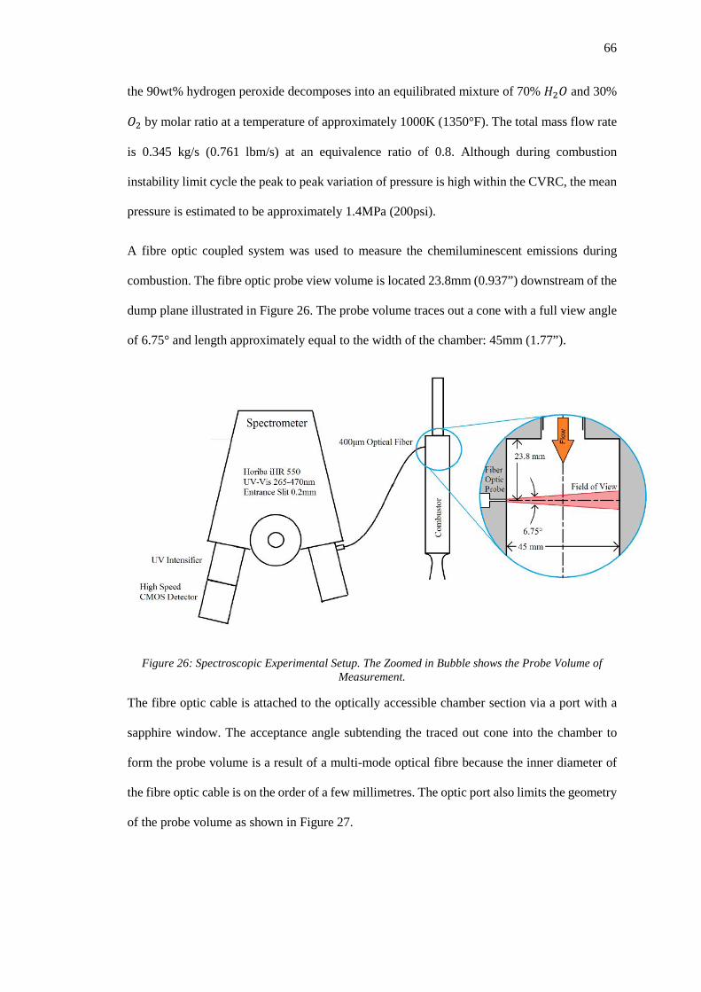
66
the 90wt% hydrogen peroxide decomposes into an equilibrated mixture of 70% 𝐻𝐻2𝐶𝐶 and 30%
𝐶𝐶2 by molar ratio at a temperature of approximately 1000K (1350°F). The total mass flow rate
is 0.345 kg/s (0.761 lbm/s) at an equivalence ratio of 0.8. Although during combustion
instability limit cycle the peak to peak variation of pressure is high within the CVRC, the mean
pressure is estimated to be approximately 1.4MPa (200psi).
A fibre optic coupled system was used to measure the chemiluminescent emissions during
combustion. The fibre optic probe view volume is located 23.8mm (0.937”) downstream of the
dump plane illustrated in Figure 26. The probe volume traces out a cone with a full view angle
of 6.75° and length approximately equal to the width of the chamber: 45mm (1.77”).
Figure 26: Spectroscopic Experimental Setup. The Zoomed in Bubble shows the Probe Volume of Measurement.
The fibre optic cable is attached to the optically accessible chamber section via a port with a
sapphire window. The acceptance angle subtending the traced out cone into the chamber to
form the probe volume is a result of a multi-mode optical fibre because the inner diameter of
the fibre optic cable is on the order of a few millimetres. The optic port also limits the geometry
of the probe volume as shown in Figure 27.
67
Figure 27: Fibre Optic Port Design.
A Horiba iHR 550 spectrometer was used. The entrance slit used was 0.2mm with a diffraction
grating of 150 grooves/mm. This allowed data to be collected at a spectral resolution of ~10-
12nm. The spectral range measured was from 265-470nm, which collected data from the 𝐶𝐶𝐻𝐻∗,
𝐶𝐶𝐻𝐻∗ and 𝐶𝐶𝐶𝐶2∗ UV-Vis emission bands of interest. The data was collected by an intensified high
resolution CMOS camera at 20000 frames per second.
3.2 Optical Model
To make the experiment and CFD computations directly comparable a spectroscopic model
was produced. The model was based on the data of the CFD computations. The computational
model is an axisymmetric 2D domain with quad elements. The information is centred in each
cell. The computational domain is outlined and represented below in Figure 28.

68
Figure 28: Computationally Modelled Domain relative to Experimental Setup.
3.2.1 Physical Mechanisms in Model
Because the information within the CFD domain is discretized and cell centred, the physics of
spectroscopy must be discretized to conform to a continuum domain. Each cell centred point
represents information regarding the state of the fluid, such as pressure, temperature, species
mass fraction, etc. By utilizing the given information in each cell a new domain where each cell
centred point acts as an optical emitter and absorber per spectral frequency. In reality the
domain can be considered a diffuse emitter of light, but because of the discretization of the
computational domain each point can be assumed to emit light in all directions depending on
the nature and abundance of the constituents at that point. The radiance per rotational level,
adapted from Equation 71 is given by:
𝐼𝐼0𝑣𝑣′,𝑣𝑣",𝐽𝐽′,𝐽𝐽"
= 𝐸𝐸𝑣𝑣′,𝑣𝑣",𝐽𝐽′,𝐽𝐽"𝐴𝐴𝑣𝑣′,𝑣𝑣",𝐽𝐽′,𝐽𝐽"𝑁𝑁𝑣𝑣′,𝐽𝐽′ (101)
The radiance is represented by 𝐼𝐼0 � 𝑊𝑊𝑚𝑚3.𝑟𝑟𝑟𝑟
�, the photon energy is given by 𝐸𝐸𝑣𝑣′,𝑣𝑣",𝐽𝐽′,𝐽𝐽" (𝐽𝐽), the
Einstein coefficient of spontaneous emission per set of rovibrational levels is given by
𝐴𝐴𝑣𝑣′,𝑣𝑣",𝐽𝐽′,𝐽𝐽" (𝑠𝑠−1) and the number density of emitters at the specific rovibrational state is given

69
by 𝑁𝑁𝑣𝑣′,𝐽𝐽′(𝑔𝑔−3). The attenuated radiance due to absorption in the basic form of the discretized
Beer-Lambert Law, from 87, is given by:
𝐼𝐼(𝑑𝑑𝑧𝑧) = 𝐼𝐼0 exp(−𝐾𝐾𝜈𝜈𝑔𝑔(𝜈𝜈 + 𝑑𝑑𝜈𝜈 )𝑑𝑑𝑧𝑧) (102)
The absorption per wavelength at each cell centre can be expressed using a discretized form of
the Beer-Lambert Law as shown below in Figure 29.
Figure 29: Discretized Form of the Beer-Lambert Law for Cell Centred Data.
From Figure 29, Ω represents the solid angle fraction of the incident EM ray 𝐼𝐼𝑛𝑛. The resultant
ray 𝐼𝐼𝑛𝑛+1 is the combination of the absorption at the cell centre of 𝐼𝐼𝑛𝑛over an optical path length
𝑑𝑑𝑧𝑧 and the emission from the cell centre. The attenuation of the incident EM ray is the product
of the frequency line strength of absorption 𝐾𝐾𝜈𝜈 and the normalized line profile 𝑔𝑔(𝜈𝜈 + 𝑑𝑑𝜈𝜈). Thus
the resultant emission can be expressed as 𝐼𝐼𝑛𝑛+1 = 𝐼𝐼𝑛𝑛(𝑑𝑑𝑧𝑧) + 𝐼𝐼0. The detuning of the frequency
at the line centre results in 𝑑𝑑𝜈𝜈 = 0 → 𝑔𝑔(𝜈𝜈).
If the Beer-Lambert law is rewritten to express the absorption fraction, then from Equation 102:
𝛼𝛼 = 1 −
𝐼𝐼(𝑑𝑑𝑧𝑧)𝐼𝐼0
= 1 − exp(−𝐾𝐾𝑣𝑣𝑔𝑔(𝜈𝜈 + 𝑑𝑑𝜈𝜈)𝑑𝑑𝑧𝑧) (103)
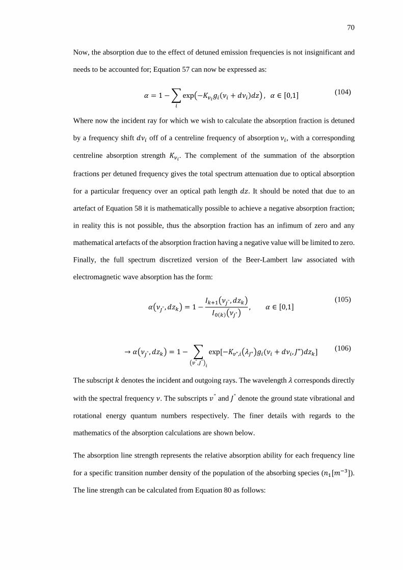
70
Now, the absorption due to the effect of detuned emission frequencies is not insignificant and
needs to be accounted for; Equation 57 can now be expressed as:
𝛼𝛼 = 1 −� exp�−𝐾𝐾𝑣𝑣𝑖𝑖𝑔𝑔𝑖𝑖(𝜈𝜈𝑖𝑖 + 𝑑𝑑𝜈𝜈𝑖𝑖)𝑑𝑑𝑧𝑧� , 𝛼𝛼 ∈ [0,1]𝑖𝑖
(104)
Where now the incident ray for which we wish to calculate the absorption fraction is detuned
by a frequency shift 𝑑𝑑𝜈𝜈𝑖𝑖 off of a centreline frequency of absorption 𝜈𝜈𝑖𝑖, with a corresponding
centreline absorption strength 𝐾𝐾𝜈𝜈𝑖𝑖. The complement of the summation of the absorption
fractions per detuned frequency gives the total spectrum attenuation due to optical absorption
for a particular frequency over an optical path length 𝑑𝑑𝑧𝑧. It should be noted that due to an
artefact of Equation 58 it is mathematically possible to achieve a negative absorption fraction;
in reality this is not possible, thus the absorption fraction has an infimum of zero and any
mathematical artefacts of the absorption fraction having a negative value will be limited to zero.
Finally, the full spectrum discretized version of the Beer-Lambert law associated with
electromagnetic wave absorption has the form:
𝛼𝛼�𝜈𝜈𝐽𝐽" ,𝑑𝑑𝑧𝑧𝑖𝑖� = 1 −
𝐼𝐼𝑖𝑖+1�𝜈𝜈𝐽𝐽" ,𝑑𝑑𝑧𝑧𝑖𝑖�𝐼𝐼0(𝑖𝑖)�𝜈𝜈𝐽𝐽"�
, 𝛼𝛼 ∈ [0,1]
(105)
→ 𝛼𝛼�𝜈𝜈𝐽𝐽" ,𝑑𝑑𝑧𝑧𝑖𝑖� = 1 − � exp [−𝐾𝐾𝑣𝑣",𝑖𝑖�𝜆𝜆𝐽𝐽"�𝑔𝑔𝑖𝑖(𝜈𝜈𝑖𝑖 + 𝑑𝑑𝜈𝜈𝑖𝑖, 𝐽𝐽")𝑑𝑑𝑧𝑧𝑖𝑖]�𝑣𝑣",𝐽𝐽"�𝑖𝑖
(106)
The subscript 𝑘𝑘 denotes the incident and outgoing rays. The wavelength 𝜆𝜆 corresponds directly
with the spectral frequency 𝜈𝜈. The subscripts 𝑣𝑣" and 𝐽𝐽" denote the ground state vibrational and
rotational energy quantum numbers respectively. The finer details with regards to the
mathematics of the absorption calculations are shown below.
The absorption line strength represents the relative absorption ability for each frequency line
for a specific transition number density of the population of the absorbing species (𝑛𝑛1[𝑔𝑔−3]).
The line strength can be calculated from Equation 80 as follows:
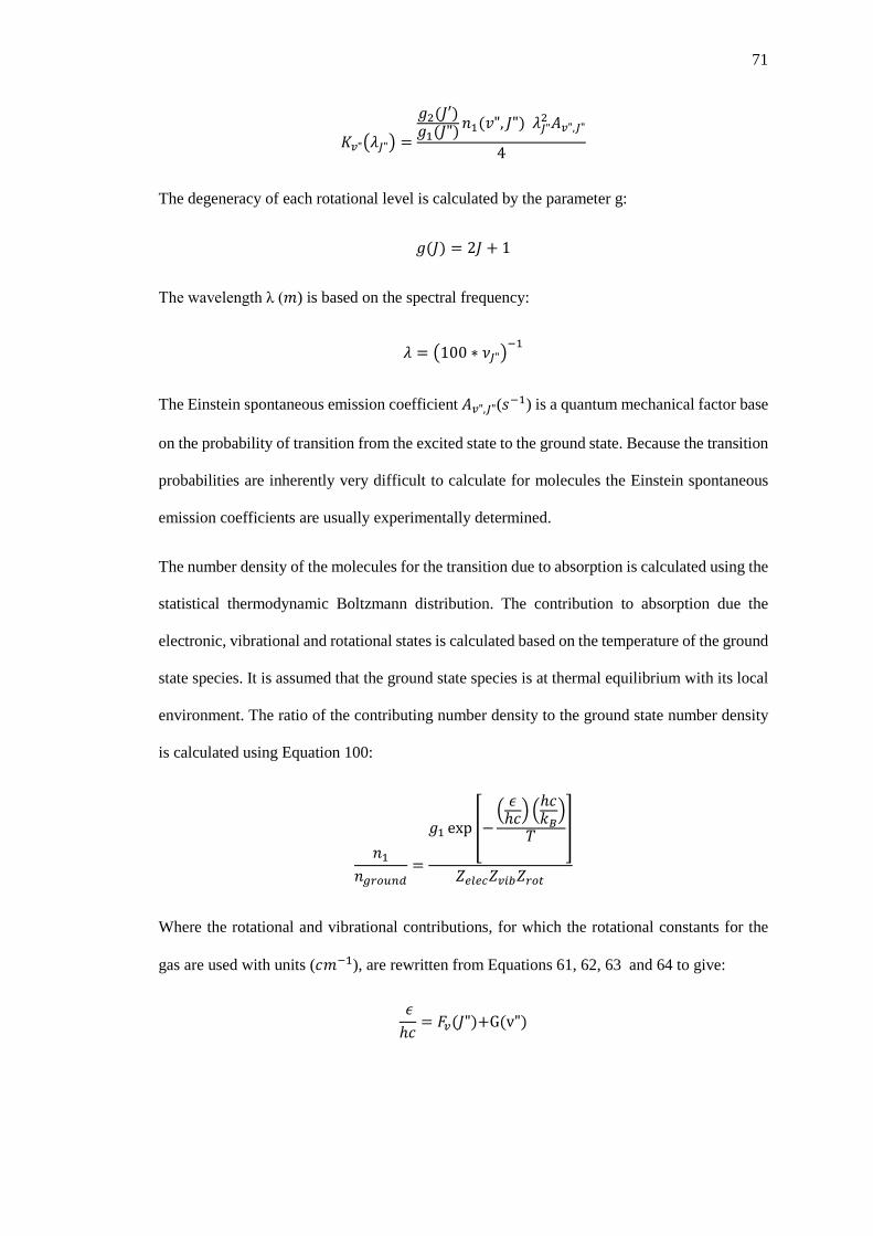
71
𝐾𝐾𝑣𝑣"�𝜆𝜆𝐽𝐽"� =
𝑔𝑔2(𝐽𝐽′)𝑔𝑔1(𝐽𝐽")𝑛𝑛1(𝑣𝑣", 𝐽𝐽") 𝜆𝜆𝐽𝐽"
2 𝐴𝐴𝑣𝑣",𝐽𝐽"
4
The degeneracy of each rotational level is calculated by the parameter g:
𝑔𝑔(𝐽𝐽) = 2𝐽𝐽 + 1
The wavelength λ (𝑔𝑔) is based on the spectral frequency:
𝜆𝜆 = �100 ∗ 𝜈𝜈𝐽𝐽"�−1
The Einstein spontaneous emission coefficient 𝐴𝐴𝑣𝑣",𝐽𝐽"(𝑠𝑠−1) is a quantum mechanical factor base
on the probability of transition from the excited state to the ground state. Because the transition
probabilities are inherently very difficult to calculate for molecules the Einstein spontaneous
emission coefficients are usually experimentally determined.
The number density of the molecules for the transition due to absorption is calculated using the
statistical thermodynamic Boltzmann distribution. The contribution to absorption due the
electronic, vibrational and rotational states is calculated based on the temperature of the ground
state species. It is assumed that the ground state species is at thermal equilibrium with its local
environment. The ratio of the contributing number density to the ground state number density
is calculated using Equation 100:
𝑛𝑛1𝑛𝑛𝑔𝑔𝑟𝑟𝑡𝑡𝑢𝑢𝑛𝑛𝑑𝑑
=
𝑔𝑔1 exp �−� 𝜖𝜖ℎ𝑔𝑔� �
ℎ𝑔𝑔𝑘𝑘𝐵𝐵�
𝑇𝑇 �
𝑍𝑍𝑒𝑒𝑏𝑏𝑒𝑒𝑐𝑐𝑍𝑍𝑣𝑣𝑖𝑖𝑏𝑏𝑍𝑍𝑟𝑟𝑡𝑡𝑡𝑡
Where the rotational and vibrational contributions, for which the rotational constants for the
gas are used with units (𝑔𝑔𝑔𝑔−1), are rewritten from Equations 61, 62, 63 and 64 to give:
𝜖𝜖ℎ𝑔𝑔
= 𝐹𝐹𝑣𝑣(𝐽𝐽")+G(v")
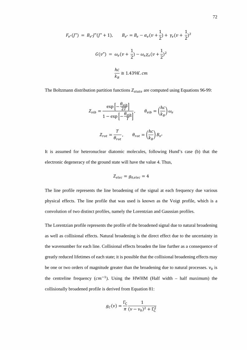
72
𝐹𝐹𝑣𝑣"(𝐽𝐽") = 𝐵𝐵𝑣𝑣"𝐽𝐽"(𝐽𝐽" + 1), 𝐵𝐵𝑣𝑣" = 𝐵𝐵𝑒𝑒 − 𝛼𝛼𝑒𝑒(𝑣𝑣 +12
) + 𝛾𝛾𝑒𝑒(𝑣𝑣 + 12
)2
𝐺𝐺(𝑣𝑣") = 𝜔𝜔𝑒𝑒(𝑣𝑣 + 12
) −𝜔𝜔𝑒𝑒𝜒𝜒𝑒𝑒(𝑣𝑣 +12
)2
ℎ𝑔𝑔𝑘𝑘𝐵𝐵
≅ 1.439𝐾𝐾. 𝑔𝑔𝑔𝑔
The Boltzmann distribution partition functions 𝑍𝑍𝑟𝑟𝑡𝑡𝑎𝑎𝑡𝑡𝑒𝑒 are computed using Equations 96-99:
𝑍𝑍𝑣𝑣𝑖𝑖𝑏𝑏 =exp �−𝑐𝑐𝑣𝑣𝑖𝑖𝑏𝑏2𝑇𝑇 �
1 − exp �−𝑐𝑐𝑣𝑣𝑖𝑖𝑏𝑏𝑇𝑇 �, 𝑐𝑐𝑣𝑣𝑖𝑖𝑏𝑏 = �
ℎ𝑔𝑔𝑘𝑘𝐵𝐵�𝜔𝜔𝑒𝑒
𝑍𝑍𝑟𝑟𝑡𝑡𝑡𝑡 =𝑇𝑇𝑐𝑐𝑟𝑟𝑡𝑡𝑡𝑡
, 𝑐𝑐𝑟𝑟𝑡𝑡𝑡𝑡 = �ℎ𝑔𝑔𝑘𝑘𝐵𝐵�𝐵𝐵𝑣𝑣"
It is assumed for heteronuclear diatomic molecules, following Hund’s case (b) that the
electronic degeneracy of the ground state will have the value 4. Thus,
𝑍𝑍𝑒𝑒𝑏𝑏𝑒𝑒𝑐𝑐 = 𝑔𝑔0,𝑒𝑒𝑏𝑏𝑒𝑒𝑐𝑐 = 4
The line profile represents the line broadening of the signal at each frequency due various
physical effects. The line profile that was used is known as the Voigt profile, which is a
convolution of two distinct profiles, namely the Lorentzian and Gaussian profiles.
The Lorentzian profile represents the profile of the broadened signal due to natural broadening
as well as collisional effects. Natural broadening is the direct effect due to the uncertainty in
the wavenumber for each line. Collisional effects broaden the line further as a consequence of
greatly reduced lifetimes of each state; it is possible that the collisional broadening effects may
be one or two orders of magnitude greater than the broadening due to natural processes. 𝜈𝜈0 is
the centreline frequency (𝑔𝑔𝑔𝑔−1). Using the HWHM (Half width – half maximum) the
collisionally broadened profile is derived from Equation 81:
𝑔𝑔𝐶𝐶(𝜈𝜈) =ΓC𝜋𝜋
1(𝜈𝜈 − 𝜈𝜈0)2 + ΓC2
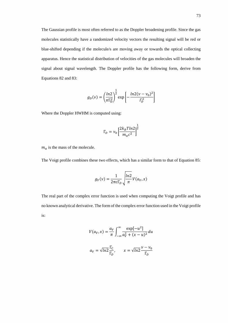
73
The Gaussian profile is most often referred to as the Doppler broadening profile. Since the gas
molecules statistically have a randomized velocity vectors the resulting signal will be red or
blue-shifted depending if the molecule/s are moving away or towards the optical collecting
apparatus. Hence the statistical distribution of velocities of the gas molecules will broaden the
signal about signal wavelength. The Doppler profile has the following form, derive from
Equations 82 and 83:
𝑔𝑔𝐷𝐷(𝜈𝜈) = �𝑔𝑔𝑛𝑛2𝜋𝜋ΓD2
�
12
exp �−𝑔𝑔𝑛𝑛2(𝜈𝜈 − 𝜈𝜈0)2
𝛤𝛤𝐷𝐷2�
Where the Doppler HWHM is computed using:
Γ𝐷𝐷 = 𝜈𝜈0 �2𝑘𝑘𝐵𝐵𝑇𝑇𝑔𝑔𝑛𝑛2𝑔𝑔𝑎𝑎𝑔𝑔2
�12
𝑔𝑔𝑎𝑎 is the mass of the molecule.
The Voigt profile combines these two effects, which has a similar form to that of Equation 85:
𝑔𝑔𝑉𝑉(𝜈𝜈) =1
2πcΓ𝐷𝐷�𝑔𝑔𝑛𝑛2𝜋𝜋𝑃𝑃(𝑎𝑎𝑉𝑉 ,𝑥𝑥)
The real part of the complex error function is used when computing the Voigt profile and has
no known analytical derivative. The form of the complex error function used in the Voigt profile
is:
𝑃𝑃(𝑎𝑎𝑉𝑉 ,𝑥𝑥) =𝑎𝑎𝑉𝑉𝜋𝜋�
exp[−𝐹𝐹2]𝑎𝑎𝑉𝑉2 + (𝑥𝑥 − 𝐹𝐹)2
𝑑𝑑𝐹𝐹∞
−∞
𝑎𝑎𝑉𝑉 = √𝑔𝑔𝑛𝑛2ΓCΓ𝐷𝐷
, 𝑥𝑥 = √𝑔𝑔𝑛𝑛2𝜈𝜈 − 𝜈𝜈0Γ𝐷𝐷
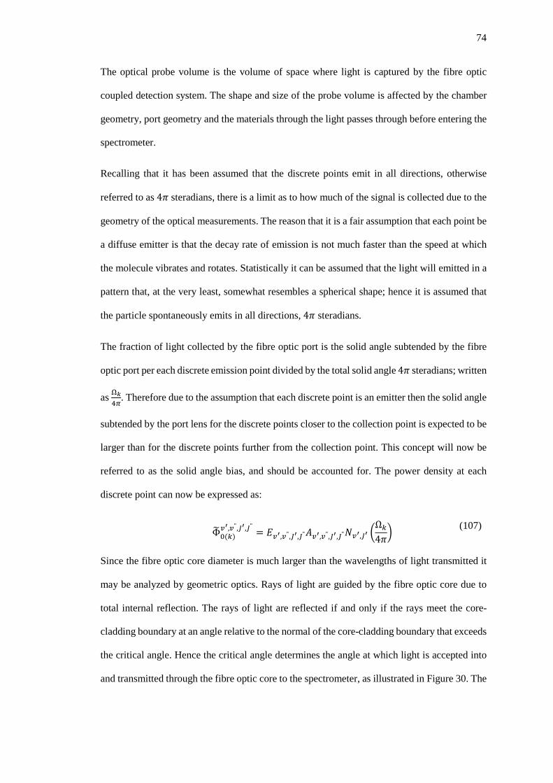
74
The optical probe volume is the volume of space where light is captured by the fibre optic
coupled detection system. The shape and size of the probe volume is affected by the chamber
geometry, port geometry and the materials through the light passes through before entering the
spectrometer.
Recalling that it has been assumed that the discrete points emit in all directions, otherwise
referred to as 4𝜋𝜋 steradians, there is a limit as to how much of the signal is collected due to the
geometry of the optical measurements. The reason that it is a fair assumption that each point be
a diffuse emitter is that the decay rate of emission is not much faster than the speed at which
the molecule vibrates and rotates. Statistically it can be assumed that the light will emitted in a
pattern that, at the very least, somewhat resembles a spherical shape; hence it is assumed that
the particle spontaneously emits in all directions, 4𝜋𝜋 steradians.
The fraction of light collected by the fibre optic port is the solid angle subtended by the fibre
optic port per each discrete emission point divided by the total solid angle 4𝜋𝜋 steradians; written
as Ω𝑘𝑘4𝜋𝜋
. Therefore due to the assumption that each discrete point is an emitter then the solid angle
subtended by the port lens for the discrete points closer to the collection point is expected to be
larger than for the discrete points further from the collection point. This concept will now be
referred to as the solid angle bias, and should be accounted for. The power density at each
discrete point can now be expressed as:
Φ�0(𝑖𝑖)𝑣𝑣′,𝑣𝑣",𝐽𝐽′,𝐽𝐽"
= 𝐸𝐸𝑣𝑣′,𝑣𝑣",𝐽𝐽′,𝐽𝐽"𝐴𝐴𝑣𝑣′,𝑣𝑣",𝐽𝐽′,𝐽𝐽"𝑁𝑁𝑣𝑣′,𝐽𝐽′ �Ω𝑖𝑖4𝜋𝜋� (107)
Since the fibre optic core diameter is much larger than the wavelengths of light transmitted it
may be analyzed by geometric optics. Rays of light are guided by the fibre optic core due to
total internal reflection. The rays of light are reflected if and only if the rays meet the core-
cladding boundary at an angle relative to the normal of the core-cladding boundary that exceeds
the critical angle. Hence the critical angle determines the angle at which light is accepted into
and transmitted through the fibre optic core to the spectrometer, as illustrated in Figure 30. The

75
acceptance angle naturally forms a conic geometry preceding the entrance to the optical fibre
core.
Figure 30: Ray Traces and Acceptance Cone for a Multimode Fibre Optic Cable [50].
Since the fibre optic cable is not flush couple with the interior of the chamber wall, the optic
port geometry will influence the acceptance cone and could be the limiting factor on the size
of the probe volume. Geometrically, as seen in Figure 27, the further the fibre optic cable is
coupled from the inner chamber wall the more the optic port limits the volume of emitters
measurable by the spectrometer. The optic port limits the acceptance angle of light from the
combustion chamber. If the power of light carried by the optic fibre approaches 1W or more
can induce Stokes fields within the fibre, due to the nonlinearity of silica molecules.
Furthermore, the index of refraction from the sapphire window is not the same as the
combustion medium, and certainly different from that of air. The refractive index of the lens
is expected to affect the acceptance angle; because the optical medium inside the chamber is
dynamic during combustion and the nature of the polarizability of the combustion medium is
unpredictable so it may not be good to assume that the refractive index of the sapphire
window is higher than the combustion medium. However, if the effective acceptance angle of
the fibre optic port is small enough or the window is physically thin then the effect due to
index of refraction may be negligible.

76
The transmissivity of the sapphire window over the spectral range 200-1000nm is well over
0.8 and the refractive index is approximately 1.8 for the band covering the peaks of OH* and
CH*.
3.2.2 Model Construction
The chamber volume has a cylindrical shape, whereas the probe volume has a conic shape. Both
shapes are axisymmetric about their longitudinal axes. It has already been assumed that the
computationally modelled data of state within the chamber is axisymmetric, hence a 2D
axisymmetric simulation. However, the axes of symmetry of the probe volume and the chamber
are orthogonal; thus the data falling inside the probe volume is not axisymmetric about the
probe volume longitudinal axis and is therefore cannot be assumed axisymmetric at all within
the probe volume. The orthogonality of the axes of symmetry is represented in Figure 31 below.
Figure 31: Orthogonal Axes of Symmetry for a Cone Intersecting a Cylinder; a Crude Analogy of the Probe Volume within the Combustor Computational Domain. The Blue Line represents the Axis of
Symmetry for the Chamber Computational Domain and the Red Line represents the Axis of Symmetry for the Probe Volume.
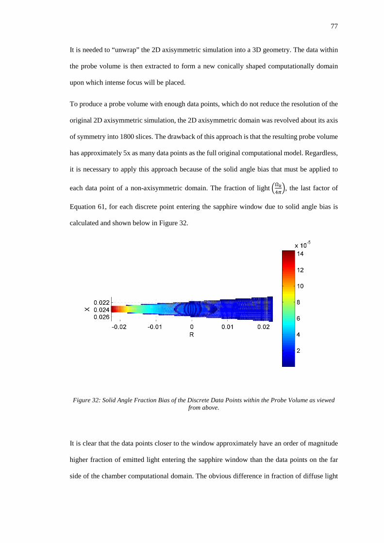
77
It is needed to “unwrap” the 2D axisymmetric simulation into a 3D geometry. The data within
the probe volume is then extracted to form a new conically shaped computationally domain
upon which intense focus will be placed.
To produce a probe volume with enough data points, which do not reduce the resolution of the
original 2D axisymmetric simulation, the 2D axisymmetric domain was revolved about its axis
of symmetry into 1800 slices. The drawback of this approach is that the resulting probe volume
has approximately 5x as many data points as the full original computational model. Regardless,
it is necessary to apply this approach because of the solid angle bias that must be applied to
each data point of a non-axisymmetric domain. The fraction of light �Ω𝑘𝑘4𝜋𝜋�, the last factor of
Equation 61, for each discrete point entering the sapphire window due to solid angle bias is
calculated and shown below in Figure 32.
Figure 32: Solid Angle Fraction Bias of the Discrete Data Points within the Probe Volume as viewed from above.
It is clear that the data points closer to the window approximately have an order of magnitude
higher fraction of emitted light entering the sapphire window than the data points on the far
side of the chamber computational domain. The obvious difference in fraction of diffuse light
78
collected from the data points with respect to location suggests that the collected emission
signal comprises mostly of emissions produced nearer to the optic port window.
To calculate the resultant emission signal collected by each discrete data point an optical path
ray trace can be utilized. The ray trace will be used to determine which data points the optical
emission will most likely travel through, and as such the state data from these points will be
used to calculate the attenuation in the signal as it approaches the optic port window.
The optic path ray trace method was first conceived with the idea to be used in a 3D probe
volume domain. A line is drawn representing the most direct optic path in 3D space to the centre
of the optic window. Finding the closest points to the ray trace was done by finding the
minimum distance from a point within a reduced set of points per layer to the optic path ray
trace. This method, in essence, is the opposite of fitting a curve to a set of 3D data with the
method of least squares. Figure 33 is a diagram of this approach.
Figure 33: Ray Trace Analogy with Optimized Method for Finding Closest Points to Ray. The Re Line represents the Ray, the Blue Dots represent the Cell Centred Discrete Points within the Probe Volume
and the Green Points are the Closest Points of the Probe Volume to the Ray.
79
The mathematics behind this approach is simply forming an equation for the ray in 3D space
using the parameterized line equation:
𝑥𝑥 − 𝑥𝑥0𝑎𝑎
=𝑏𝑏 − 𝑏𝑏0𝑏𝑏
=𝑧𝑧 − 𝑧𝑧0𝑔𝑔
(108)
Where 𝑎𝑎, 𝑏𝑏 and 𝑔𝑔 are the magnitude quantities of the vector from the initial discrete data point
of the line in 3D space < 𝑥𝑥0, 𝑏𝑏0, 𝑧𝑧0 > to the final point in space at the probe volume conical
apex. Any point along the line can be found by solving for the variables 𝑥𝑥, 𝑏𝑏 and 𝑧𝑧. To solve
for the variables a stepping method can be done through one of three Cartesian directions; it is
recommended that the chamber domain radial direction be used for the purpose of this
calculation with respect to the probe volume.
If the “unwrapping” of the 2D axisymmetric computational domain is done correctly then there
should be layers of points in the radial direction from the apex of the cone found at the optic
port window. These layers can be used as the stepping distance to sort the discrete points into
groups in order to scrutinize the distance each point lies from the ray investigated. The location
closest cell centre is determined by:
< 𝑥𝑥𝑝𝑝, 𝑏𝑏𝑝𝑝, 𝑧𝑧𝑝𝑝 > = min ��(𝑋𝑋 − 𝑥𝑥𝑖𝑖)2 + (𝑍𝑍 − 𝑧𝑧𝑖𝑖)2� , 𝑏𝑏 = 𝑏𝑏𝑖𝑖 (109)
The matrix of coordinates of the points in the radial layer 𝑏𝑏𝑖𝑖 are given by 𝑋𝑋 and 𝑍𝑍, while the
point on the ray is given by < 𝑥𝑥𝑖𝑖, 𝑏𝑏𝑖𝑖, 𝑧𝑧𝑖𝑖 >. The resulting cell centred location closest to the ray
trace for a given radial layer 𝑏𝑏𝑖𝑖 is < 𝑥𝑥𝑝𝑝, 𝑏𝑏𝑝𝑝, 𝑧𝑧𝑝𝑝 >.
Although this method proves to be quite accurate, it is extremely computationally intensive. A
reduced order method would be able to condense the data in order to reduce the memory and
computational cost. One reduced order method is to collapse all the data into a 1D domain, a
single optical path line. This approach would effectively represent the probe volume as a series
of shells with the averaged data within a shell represented by a single data point centred within
the shell. The data within the shell is volume averaged because each cell within the probe
volume domain is actually a 1800th slice of an annular cell of the 2D axisymmetric domain. The

80
annular cell is represented by and the representation of the volume of the sliced cell as shown
in Figure 34.
Figure 34: Representation of the Annular Cell in 3D of an Axisymmetric 2D Cell in Plane. The Axes of the Annular Cell are Arbitrary.
Figure 35: Generalized Volume Approach to Quadrilateral Cross Sectioned Cell.

81
The connectivity of the data node points within the original computational domain do not
always follow the same pattern or was inconsistent, therefore a general method for determining
the volume of each cell was used, this method is outlined below.
Using the reference data from Figure 35, the individual cell volume in 3D space is calculated.
Because in some cases the connecting nodes of the cell may not represent a square or rectangle
exactly, a general approach for finding the line equations that represent the boundary of the cell
in 2D space are found first. These boundary equations are then revolved about the
computational domain axis of symmetry to form the annular cell volume in 3D space. The
“artificial” probe volume data points create by revolving the plane in 3D at discrete intervals
will then have a fraction of the annular volume of the original cell based on the number of
discrete plane revolutions. The approach to the cell volume calculation is presented below.
Linear Boundary Equations for Cell:
𝑏𝑏𝑖𝑖(𝑥𝑥) = 𝑎𝑎𝑖𝑖𝑥𝑥 + 𝑏𝑏𝑖𝑖 (110)
Boundary Equation Coefficients:
𝑎𝑎1 =𝑦𝑦4 − 𝑦𝑦2𝑥𝑥4 − 𝑥𝑥2
, 𝑏𝑏1 = 𝑦𝑦4 − 𝑎𝑎1𝑥𝑥4 (111)
𝑎𝑎2 =𝑦𝑦3 − 𝑦𝑦1𝑥𝑥3 − 𝑥𝑥1
, 𝑏𝑏2 = 𝑦𝑦3 − 𝑎𝑎2𝑥𝑥3
𝑎𝑎3 =𝑦𝑦2 − 𝑦𝑦1𝑥𝑥2 − 𝑥𝑥1
, 𝑏𝑏3 = 𝑦𝑦2 − 𝑎𝑎3𝑥𝑥2
𝑎𝑎4 =𝑦𝑦4 − 𝑦𝑦3𝑥𝑥4 − 𝑥𝑥3
, 𝑏𝑏4 = 𝑦𝑦4 − 𝑎𝑎4𝑥𝑥4
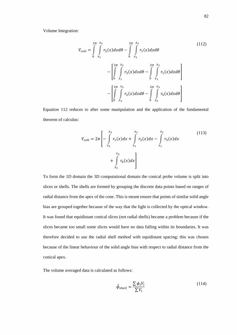
82
Volume Integration:
𝑃𝑃𝑐𝑐𝑒𝑒𝑏𝑏𝑏𝑏 = � � 𝑏𝑏2(𝑥𝑥)𝑑𝑑𝑥𝑥𝑑𝑑𝑐𝑐
𝑚𝑚4
𝑚𝑚1
2𝜋𝜋
0
− � � 𝑏𝑏1(𝑥𝑥)𝑑𝑑𝑥𝑥𝑑𝑑𝑐𝑐
𝑚𝑚4
𝑚𝑚1
2𝜋𝜋
0
− �� � 𝑏𝑏3(𝑥𝑥)𝑑𝑑𝑥𝑥𝑑𝑑𝑐𝑐
𝑚𝑚2
𝑚𝑚1
2𝜋𝜋
0
− � � 𝑏𝑏1(𝑥𝑥)𝑑𝑑𝑥𝑥𝑑𝑑𝑐𝑐
𝑚𝑚2
𝑚𝑚1
2𝜋𝜋
0
�
− �� � 𝑏𝑏2(𝑥𝑥)𝑑𝑑𝑥𝑥𝑑𝑑𝑐𝑐
𝑚𝑚4
𝑚𝑚3
2𝜋𝜋
0
− � � 𝑏𝑏4(𝑥𝑥)𝑑𝑑𝑥𝑥𝑑𝑑𝑐𝑐
𝑚𝑚4
𝑚𝑚3
2𝜋𝜋
0
�
(112)
Equation 112 reduces to after some manipulation and the application of the fundamental
theorem of calculus:
𝑃𝑃𝑐𝑐𝑒𝑒𝑏𝑏𝑏𝑏 = 2𝜋𝜋 �− � 𝑏𝑏1(𝑥𝑥)𝑑𝑑𝑥𝑥
𝑚𝑚4
𝑚𝑚2
+ � 𝑏𝑏2(𝑥𝑥)𝑑𝑑𝑥𝑥
𝑚𝑚3
𝑚𝑚1
− � 𝑏𝑏3(𝑥𝑥)𝑑𝑑𝑥𝑥
𝑚𝑚2
𝑚𝑚1
+ � 𝑏𝑏4(𝑥𝑥)𝑑𝑑𝑥𝑥
𝑚𝑚4
𝑚𝑚3
�
(113)
To form the 1D domain the 3D computational domain the conical probe volume is split into
slices or shells. The shells are formed by grouping the discrete data points based on ranges of
radial distance from the apex of the cone. This is meant ensure that points of similar solid angle
bias are grouped together because of the way that the light is collected by the optical window.
It was found that equidistant conical slices (not radial shells) became a problem because if the
slices became too small some slices would have no data falling within its boundaries. It was
therefore decided to use the radial shell method with equidistant spacing; this was chosen
because of the linear behaviour of the solid angle bias with respect to radial distance from the
conical apex.
The volume averaged data is calculated as follows:
𝜙𝜙�𝑟𝑟ℎ𝑒𝑒𝑏𝑏𝑏𝑏 =
∑𝜙𝜙𝑖𝑖𝑃𝑃𝑖𝑖∑𝑃𝑃𝑖𝑖
(114)
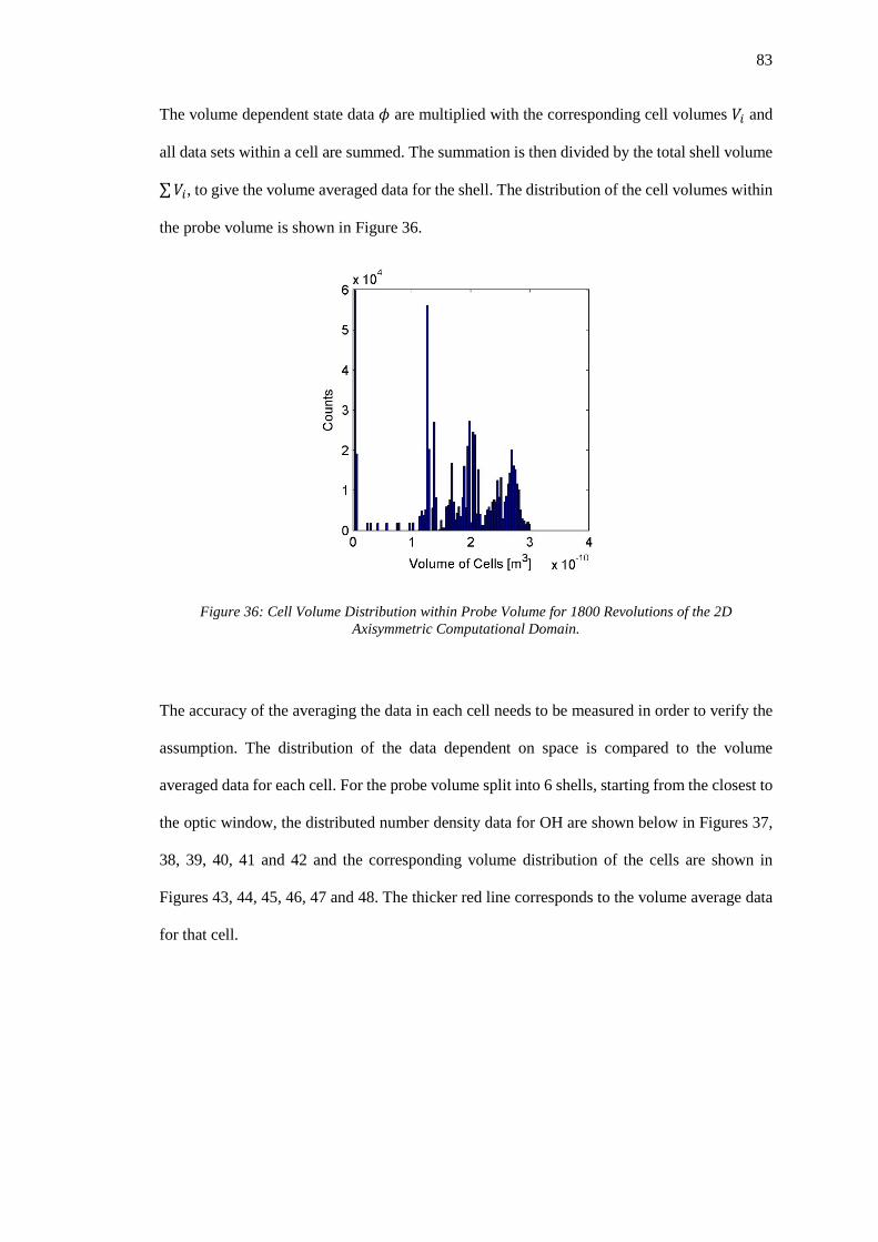
83
The volume dependent state data 𝜙𝜙 are multiplied with the corresponding cell volumes 𝑃𝑃𝑖𝑖 and
all data sets within a cell are summed. The summation is then divided by the total shell volume
∑𝑃𝑃𝑖𝑖, to give the volume averaged data for the shell. The distribution of the cell volumes within
the probe volume is shown in Figure 36.
Figure 36: Cell Volume Distribution within Probe Volume for 1800 Revolutions of the 2D Axisymmetric Computational Domain.
The accuracy of the averaging the data in each cell needs to be measured in order to verify the
assumption. The distribution of the data dependent on space is compared to the volume
averaged data for each cell. For the probe volume split into 6 shells, starting from the closest to
the optic window, the distributed number density data for OH are shown below in Figures 37,
38, 39, 40, 41 and 42 and the corresponding volume distribution of the cells are shown in
Figures 43, 44, 45, 46, 47 and 48. The thicker red line corresponds to the volume average data
for that cell.

84
Figure 37: Number Density Distribution of OH within Probe Volume. Shell 1 of 6.
Figure 38: Number Density Distribution of OH within Probe Volume. Shell 2 of 6.
Figure 39: Number Density Distribution of OH within Probe Volume. Shell 3 of 6.
Figure 40: Number Density Distribution of OH within Probe Volume. Shell 4 of 6.
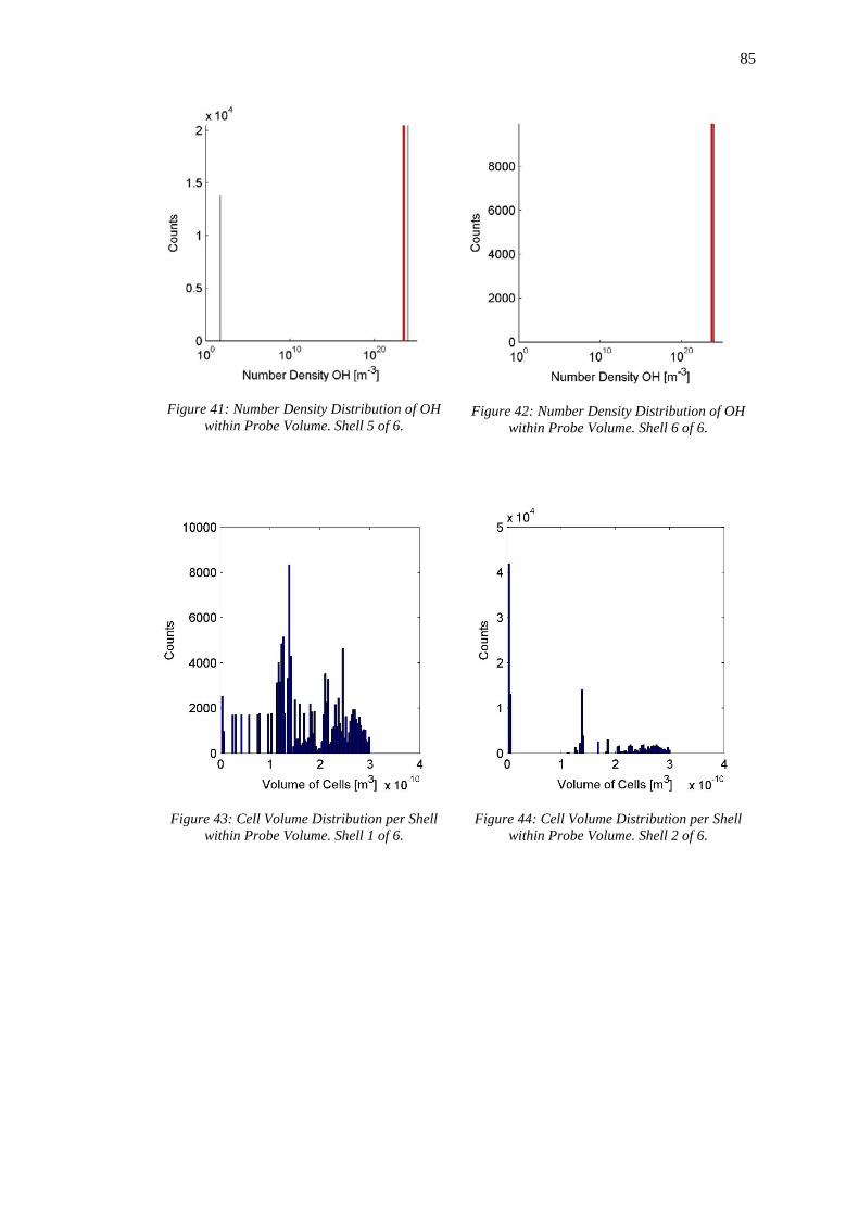
85
Figure 41: Number Density Distribution of OH within Probe Volume. Shell 5 of 6.
Figure 42: Number Density Distribution of OH within Probe Volume. Shell 6 of 6.
Figure 43: Cell Volume Distribution per Shell within Probe Volume. Shell 1 of 6.
Figure 44: Cell Volume Distribution per Shell within Probe Volume. Shell 2 of 6.

86
Figure 45: Cell Volume Distribution per Shell within Probe Volume. Shell 3 of 6.
Figure 46: Cell Volume Distribution per Shell within Probe Volume. Shell 4 of 6.
Figure 47: Cell Volume Distribution per Shell within Probe Volume. Shell 5 of 6.
Figure 48: Cell Volume Distribution per Shell within Probe Volume. Shell 6 of 6.
From Figures 37, 38, 39, 40, 41 and 42 the volume averaged mean appears to approximate the
dominant levels of number density per shell quite well. This suggests that the volume averaged
mean could be a good representation of the overall data within an acceptable confidence level.
The cell volume distribution per shell from Figures 43, 44, 45, 46, 47 and 48 do not show a
continuous distribution pattern. It is unclear what effect what the volume distribution pattern

87
will have on the data spread for the state properties. There does seem to be some sort of coherent
connection between the volume distribution and the number density distribution; this is evident
from Figures 39 and 40, and Figures 51 and 52 where the similar distribution in cell volume
per shell reflects a similar distribution of state property data distribution per shell. Since the
pattern of the behaviour could not be determine from such a small sample size the number of
shells were increased to determine if any changes would happen to the data distribution and the
severity of the change.
If the number of shells is doubled then the data spread does not compare well with enough
confidence to the approach of splitting the probe volume into 6 shells qualitatively; as shown
with Figures 49, 50, 51, 52, 53 and 54 with respect to OH number density distribution per 1D
shell volume; and Figures 55, 56, 57, 58, 59 and 60 with respect to 3D cell volume distribution
per 1D cell volume. A study was performed to ascertain what number of shells, if it were
possible, were necessary to produce an accurate result. The study was based on the emissions
produced per probe volume because that was the data of most interest. The emissions were
plotted against the variation in number of shells to determine a possible trend, depicted by
Figure 61 and Figure 62.
It is clear from Figure 61 and Figure 62 that for a probe volume split into more than
approximately 75 shells, the emissions become consistent for that specific set of data. Using a
conservative approach 100 shells were chosen to ensure the highest level of accuracy without
inducing a computational cost that was too high for this particular model.

88
Figure 49: Number Density Distribution of OH within Probe Volume. Shell 1 of 12.
Figure 50: Number Density Distribution of OH within Probe Volume. Shell 3 of 12.
Figure 51: Number Density Distribution of OH within Probe Volume. Shell 5 of 12.
Figure 52: Number Density Distribution of OH within Probe Volume. Shell 7 of 12.

89
Figure 53: Number Density Distribution of OH within Probe Volume. Shell 9 of 12.
Figure 54: Number Density Distribution of OH within Probe Volume. Shell 11 of 12.
Figure 55: Cell Volume Distribution per Shell within Probe Volume. Shell 1 of 12.
Figure 56: Cell Volume Distribution per Shell within Probe Volume. Shell 3 of 12.

90
Figure 57: Cell Volume Distribution per Shell within Probe Volume. Shell 5 of 12.
Figure 58: Cell Volume Distribution per Shell within Probe Volume. Shell 7 of 12.
Figure 59: Cell Volume Distribution per Shell within Probe Volume. Shell 9 of 12.
Figure 60: Cell Volume Distribution per Shell within Probe Volume. Shell 11 of 12.

91
Figure 61: CH* Spectrally Integrated Emission of the Probe Volume as Approximated by Varying Number of 1D Shells. The Green Line Represents the Running Mean of the Data as a Function of
Number 1D Shells.
Figure 62: OH* Spectrally Integrated Emission of the Probe Volume as Approximated by Varying Number of 1D Shells. The Green Line Represents the Running Mean of the Data as a Function of
Number 1D Shells.
It should be further noted that the distributions of the number densities of the absorbing species
with respect to OH* and CH* do not follow predictable profiles as evident by the preceding
figures. The significance of the number density distributions not following a trending profile
92
suggests that the optical absorption of the emitted radiation may be difficult to predict spatially
and temporally. From the perspective of experimental measurements the resultant line of sight
integrated signal may experience optical absorption that will be unpredictable without the use
of some sort of tomographic technique. Additionally, any emissions produced within the probe
volume will be collected without regard of the spatial location of the source and therefore the
information received will not provide any insight into any spatially resolved local processes
that may occur. Consequently, because this technique is line-of-sight integrated it severely
limits the ability of the measurements to provide quantitative data about the heat release and
associated processes.
3.2.3 Normalized Spectrum Line Profile Estimation
It is unclear from the experimental data, numerical data or from literature whether the
normalized line profile of the optical spectrum emitted from the CVRC chamber is dominated
by collisional or Doppler effects. Therefore, there is no fundamental basis upon which an
assumption can made to model the spectrum one way or the other. Thus, a Voigt profile, given
by Equation 85, was chosen, which is the convolution of the Doppler and homogeneous line
broadening profiles, Gaussian and Lorentzian profiles respectively. The drawback of this
approach is the calculation of the Voigt profile in the general sense. The Voigt profile is
calculated by integrating the complex error function, which does not have a known analytical
solution. There are a number of numerical approaches to solving the problem associated with
calculating the Voigt profile, the main basic approach is discussed here.
The most popular method of approximating the Voigt function today is the Humlicek 12-point
method [51]. The method is a 12 point Gauss-Hermite quadrature of the integral of the complex
error function in Equation 86. The Hermite function used to interpolate the function between
the points is the physicists’ version and not the cubic polynomial. The quadrature produces a
function that generally follows the Voigt function within a relative error of approximately 10−5.

93
A computational algorithm written and submitted to the Matlab website Mathworks by Dr. N.
Cherkasov was used to numerically compute the Voigt profile. The algorithm was programmed
into a set of two functions: the Voigt profile function, which outputs the numerical values of
the Voigt profile at a centreline frequency with a distributed range of detuned frequencies; and
the numerical integration function of the complex error function. The real part of the integrated
complex error function is used to calculate the Voigt profile. The algorithm uses the half-width-
half-maximum (HWHM) values of the Gaussian and Lorentzian line shapes as opposed to the
conventional full-width-half-maximum (FWHM) values. The programmed function in Matlab
is found in Appendix B.
There have various advancements in optimizing the numerical approximation to the Voigt
profile in terms of accuracy and speed. Most methods approach with variances in the method
of how the complex error function is integrated with Gauss-Hermite quadrature. The most
optimal method that was found to date was by Letchworth and Benner (2007) [52], which uses
further Taylor series expansions for the parts of the Voigt profile which have the highest
gradient and that are furthest from the line centre. This method seems far superior to Humlicek’s
method, but for the purpose of this model where the experimental spectral resolution is low and
the uncertainty in the linewidths is high Humlicek’s method is sufficient.
Due to the uncertainty of the exact constituents within the flame the collisional linewidth is
difficult to predict. The prediction of the dephasing of the signal due to collisions relies on the
knowledge of which collision partners are present and in what abundance. The information that
is known which can affect the collisional linewidth is the overall static pressure within the
system. There is some data about the collisional linewidth with regards to OH* emissions in
atmospheric flames; the FWHM was reported to be approximately 0.1𝑔𝑔𝑔𝑔−1. To approximate
the collisional linewidth at higher pressures a linear extrapolation of the collisional linewidth
with pressure was taken; since the number density scales linearly with pressure for an ideal gas,
it may be assumed that the number of collisions between molecules might also scale linearly

94
with pressure. However, since the collisional partners for the oxidation of methane with
decomposed hydrogen peroxide are quite different to that of air a slightly more scientific
approach was used.
Using the approximate mean temperature within the combustor to be 2400K the emission
spectrum of OH was simulated using Lifbase [53], a spectrum database and simulator. Doppler
and collisional broadening were included, corresponding to a pressure of 15 atm. The spectral
resolution was set to 1.2nm with 10% noise in applied to the raw spectrum. Figure 63 shows
the spectral output simulated by Lifbase. A Voigt line shape was used where the Doppler and
collisional linewidths are approximately 0.03 and 0.98 cm−1 respectively. A time averaged
emission spectrum ws collected from the CVRC experiment, displayed in Figure 64. The
spectral range is from 270nm to 470nm. The OH* emission is centred at approximately 310nm.
Qualitatively the pair of spectrums compare quite well for the emission produced by the
hydroxyl radical. It was decided to use the collisional linewidth of 1𝑔𝑔𝑔𝑔−1 as the collsional
linewidth parameter, until data with regards to the collisional effects within the CVRC become
available.

95
Figure 63: Emission Spectral Simulation of OH Emission at T=2400K and P=15atm. A Voigt Line Shape was used, Doppler and Collisional Linewidths are approximately 0.03 and 0.98 𝑔𝑔𝑔𝑔−1
respectively [53].
Figure 64: Time Averaged Emission Spectrum from the CVRC Experiment.

96
3.2.4 Numerical Considerations
Calculations involving finite or floating point numbers have finite errors associated with them.
The operations involving very big and/or very small numbers leads to a reduction in the
precision of the numerical computations. The addition or subtraction of numbers with a high
difference in the order of magnitude will result in a loss of precision of the smaller number,
even to the point where the operation involving the smaller number may become negligible
with regards to the precision that the computer can handle. Other considerations involve the
multiplication and division of large and small numbers; the operation may not necessarily cause
a loss in precision, but if the product or quotient becomes too large or too small then the value
may fall outside the range of finite numbers that the computer can handle.
The scenario whereby a finite number is too large for the computer to represent is called
overflow, and the scenario whereby a finite number is too small for the computer to represent
is called underflow. Matlab deals with these cases by rounding the numbers off to an assigned
special number which represent the boundary of the range of finite numbers that the computer
can represent. For the case of underflow the variable’s value is rounded to zero and for the case
of overflow the variable’s value is assigned an infinite vale “Inf”.
For a double precision 64 bit binary architecture, according to the IEEE standard, the largest
number that can be represented is 10308, while the smallest number representable by the
computer is 10−323. The precision of this floating point format is approximately 16 decimal
digits. The numbers are represented by the computer, in base 10 mathematical format, as:
𝑥𝑥1.𝑥𝑥2𝑥𝑥3𝑥𝑥4𝑥𝑥5𝑥𝑥6𝑥𝑥7𝑥𝑥8𝑥𝑥9𝑥𝑥10𝑥𝑥11𝑥𝑥12𝑥𝑥13𝑥𝑥14𝑥𝑥15 × 10−𝑒𝑒𝑚𝑚𝑝𝑝𝑡𝑡𝑛𝑛𝑒𝑒𝑛𝑛𝑡𝑡
, where each variable represent a digit in the decimal format.
To reduce the loss of precision it is sometimes helpful to operate sets of numbers with similar
precision and order of magnitude in a particular order; such adding large numbers together

97
before multiplying the group instead of multiplying each number first and then adding them,
etc.
Although some of the constants have a high numerical value and others very small, the double
precision floating point format is adequate in representing the numbers and calculations of this
model with sufficient precision.
3.3 Summary of Assumptions and Constants
Before the model can be verified a summary of all assumptions will be made below to ensure
clarity and meaning towards the results of the model. Each assumption will be stated with a
summarised reason as to why such an assumption was made.
Table 10: Spectroscopic Model Assumptions
Assumption Reason
1. OH* and CH* in thermal
equilibrium with combustion
medium.
An approximation made in order to
calculate spectra.
2. Probe volume compressed to 1D
domain.
Reduction in computational time;
enough shells is thought to approximate
the level of emissions sufficiently.
3. Each discrete point in probe volume
can be approximated as an
emitter/absorber.
Discretization approximation to mimic a
continuous domain.

98
4. Each discrete point emits in all
directions.
The rate of decay is much faster than the
rotational speed of the molecule; an
ensemble of particles also have
randomized orientations.
5. Absorption due to other species
initially neglected.
Focus on self-absorption effects.
6. Emission profile set as
monochromatic.
Focus on absorption effects; unclear
whether emissions are quantifiably
comparable to experimental data.
7. Absorption spectrum approximated
with Voigt profile.
Effects due to Doppler and collisional
processes unknown ab initio.
8. Broadening of absorption spectrum
approximate to be 1𝑔𝑔𝑔𝑔−1.
Comparable to Lifbase simulation; also
linearly extrapolated from atmospheric
conditions.
9. Stimulated emission negligible. Absorption is not saturated enough at
each discrete point from
chemiluminescent emissions.

99
The constants stated for use in the model are listed below. Each constant has a mean value and
a standard deviation.
Table 11: Summary of Constants [2].
Constant Mean Value Standard Deviation
𝑅𝑅𝑢𝑢 8.3144621𝐽𝐽
𝑔𝑔𝑔𝑔𝑔𝑔.𝐾𝐾 0.0000075
𝐽𝐽𝑔𝑔𝑔𝑔𝑔𝑔.𝐾𝐾
𝑘𝑘𝐵𝐵 1.3806488 × 10⁻²³𝐽𝐽𝐾𝐾
0.0000013 × 10⁻²³𝐽𝐽𝐾𝐾
𝑁𝑁𝐴𝐴 6.02214129 × 10²³𝑔𝑔𝑔𝑔𝑔𝑔−1 0.00000027 × 10²³𝑔𝑔𝑔𝑔𝑔𝑔−1
𝑔𝑔 299792458𝑔𝑔𝑠𝑠
Exact
ℎ 6.62606957 × 10⁻³⁴𝐽𝐽. 𝑠𝑠 0.00000029 × 10⁻³⁴𝐽𝐽. 𝑠𝑠
𝜖𝜖0 8.854187817 … × 10−12𝐹𝐹𝑔𝑔
Exact
𝑞𝑞 1.602176565 × 10⁻¹⁹𝐶𝐶 0.000000035 × 10⁻¹⁹𝐶𝐶
𝑔𝑔𝑒𝑒 9.10938291 × 10⁻³¹𝑘𝑘𝑔𝑔 0.00000040 × 10⁻³¹𝑘𝑘𝑔𝑔
ℳ𝑂𝑂𝐻𝐻 17.00734 𝑔𝑔/𝑔𝑔𝑔𝑔𝑔𝑔 0.00037 𝑔𝑔/𝑔𝑔𝑔𝑔𝑔𝑔
ℳ𝐶𝐶𝐻𝐻 13.01864 𝑔𝑔/𝑔𝑔𝑔𝑔𝑔𝑔 0.00087 𝑔𝑔/𝑔𝑔𝑔𝑔𝑔𝑔

100
3.4 Model Verification Process
An example of the process of calculating the absorption along a path length is done. The basic
characteristics of the process and the behaviour of the calculation towards varying parameters
provides evidence of a need to study the sensitivity of the model to various parameters.
An investigation of the model sensitivity to different state parameters of interest is conducted
to ensure model stability and accuracy. The sensitivity of the model to perturbations with
respect to various parameters was investigated.
3.4.1 Example of Analytical Absorption Calculation
Assumptions:
• Monochromatic absorption on line centre.
• Collisional linewidth (FWHM) has a value of 1 𝑔𝑔𝑔𝑔−1.
• Gas radical is OH, line with strongest spontaneous transition was used 𝑃𝑃1(1.5) [44].
• Optical path length of 0.045m.
• Homogeneous number density through optical path length.
Parameters:
• 𝑛𝑛𝑂𝑂𝐻𝐻 = 5 ∗ 1021𝑔𝑔−3
• 𝑣𝑣" = 0, 𝐽𝐽" = 1.5
• Γ𝐶𝐶 = 12
𝑔𝑔𝑔𝑔−1
• 𝜈𝜈0 = 32440.58𝑔𝑔𝑔𝑔−1
• 𝐴𝐴0,1.5 = 8.585 × 10⁵𝑠𝑠−1
• 𝑇𝑇 = 2400𝐾𝐾
• Rotational constants:
o 𝐵𝐵𝑒𝑒 = 18.89638𝑔𝑔𝑔𝑔−1
o 𝛼𝛼𝑒𝑒 = 0.725042𝑔𝑔𝑔𝑔−1
o 𝛾𝛾𝑒𝑒 = 8.3292 × 10⁻³𝑔𝑔𝑔𝑔−1
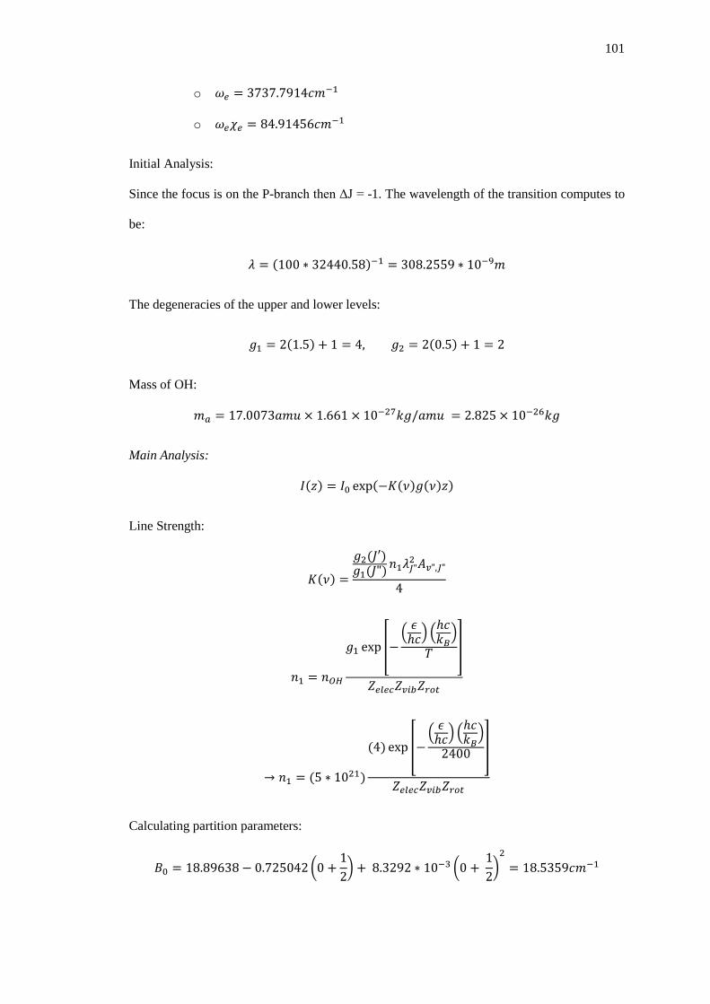
101
o 𝜔𝜔𝑒𝑒 = 3737.7914𝑔𝑔𝑔𝑔−1
o 𝜔𝜔𝑒𝑒𝜒𝜒𝑒𝑒 = 84.91456𝑔𝑔𝑔𝑔−1
Initial Analysis:
Since the focus is on the P-branch then ΔJ = -1. The wavelength of the transition computes to
be:
𝜆𝜆 = (100 ∗ 32440.58)−1 = 308.2559 ∗ 10−9𝑔𝑔
The degeneracies of the upper and lower levels:
𝑔𝑔1 = 2(1.5) + 1 = 4, 𝑔𝑔2 = 2(0.5) + 1 = 2
Mass of OH:
𝑔𝑔𝑎𝑎 = 17.0073𝑎𝑎𝑔𝑔𝐹𝐹 × 1.661 × 10⁻²⁷𝑘𝑘𝑔𝑔/𝑎𝑎𝑔𝑔𝐹𝐹 = 2.825 × 10⁻²⁶𝑘𝑘𝑔𝑔
Main Analysis:
𝐼𝐼(𝑧𝑧) = 𝐼𝐼0 exp(−𝐾𝐾(𝜈𝜈)𝑔𝑔(𝜈𝜈)𝑧𝑧)
Line Strength:
𝐾𝐾(𝜈𝜈) =
𝑔𝑔2(𝐽𝐽′)𝑔𝑔1(𝐽𝐽")𝑛𝑛1𝜆𝜆𝐽𝐽"
2 𝐴𝐴𝑣𝑣",𝐽𝐽"
4
𝑛𝑛1 = 𝑛𝑛𝑂𝑂𝐻𝐻
𝑔𝑔1 exp �−� 𝜖𝜖ℎ𝑔𝑔� �
ℎ𝑔𝑔𝑘𝑘𝐵𝐵�
𝑇𝑇 �
𝑍𝑍𝑒𝑒𝑏𝑏𝑒𝑒𝑐𝑐𝑍𝑍𝑣𝑣𝑖𝑖𝑏𝑏𝑍𝑍𝑟𝑟𝑡𝑡𝑡𝑡
→ 𝑛𝑛1 = (5 ∗ 1021)
(4) exp �−� 𝜖𝜖ℎ𝑔𝑔� �
ℎ𝑔𝑔𝑘𝑘𝐵𝐵�
2400 �
𝑍𝑍𝑒𝑒𝑏𝑏𝑒𝑒𝑐𝑐𝑍𝑍𝑣𝑣𝑖𝑖𝑏𝑏𝑍𝑍𝑟𝑟𝑡𝑡𝑡𝑡
Calculating partition parameters:
𝐵𝐵0 = 18.89638− 0.725042 �0 +12� + 8.3292 ∗ 10−3 �0 +
12�2
= 18.5359𝑔𝑔𝑔𝑔−1
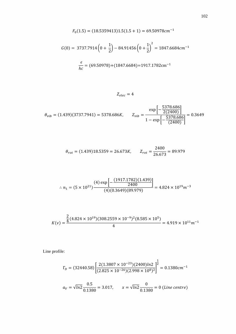
102
𝐹𝐹0(1.5) = (18.5359413)1.5(1.5 + 1) = 69.50978𝑔𝑔𝑔𝑔−1
𝐺𝐺(0) = 3737.7914 �0 + 12� − 84.91456 �0 +
12�2
= 1847.6684𝑔𝑔𝑔𝑔−1
𝜖𝜖ℎ𝑔𝑔
= (69.50978)+(1847.6684)=1917.1782cm−1
𝑍𝑍𝑒𝑒𝑏𝑏𝑒𝑒𝑐𝑐 = 4
𝑐𝑐𝑣𝑣𝑖𝑖𝑏𝑏 = (1.439)(3737.7941) = 5378.686𝐾𝐾, 𝑍𝑍𝑣𝑣𝑖𝑖𝑏𝑏 =exp �−5378.686
2(2400) �
1 − exp �−5378.686(2400) �
= 0.3649
𝑐𝑐𝑟𝑟𝑡𝑡𝑡𝑡 = (1.439)18.5359 = 26.673𝐾𝐾, 𝑍𝑍𝑟𝑟𝑡𝑡𝑡𝑡 =2400
26.673= 89.979
∴ 𝑛𝑛1 = (5 × 10²¹)(4) exp �− (1917.1782)(1.439)
2400 �
(4)(0.3649)(89.979) = 4.824 × 10¹⁹𝑔𝑔−3
𝐾𝐾(𝜈𝜈) =24 (4.824 × 10¹⁹)(308.2559 × 10⁻⁹)2(8.585 × 10⁵)
4= 4.919 × 10¹¹𝑔𝑔−1
Line profile:
Γ𝐷𝐷 = (32440.58) �2(1.3807 × 10⁻²³)(2400)𝑔𝑔𝑛𝑛2
(2.825 × 10⁻²⁶)(2.998 × 10⁸)2�
12
= 0.1380𝑔𝑔𝑔𝑔−1
𝑎𝑎𝑉𝑉 = √𝑔𝑔𝑛𝑛20.5
0.1380= 3.017, 𝑥𝑥 = √𝑔𝑔𝑛𝑛2
00.1380
= 0 (𝐿𝐿𝑖𝑖𝑛𝑛𝑒𝑒 𝑔𝑔𝑒𝑒𝑛𝑛𝑡𝑡𝑏𝑏𝑒𝑒)

103
→ 𝑃𝑃(𝑎𝑎𝑉𝑉 ,𝑥𝑥) ≅ 0.1790
𝑔𝑔𝑉𝑉(𝜈𝜈) =1
2𝜋𝜋(2.998 × 10¹⁰)0.1380�𝑔𝑔𝑛𝑛2𝜋𝜋
(0.1790) = 3.234 × 10⁻¹²
Transmissivity:
𝐼𝐼(𝑧𝑧)𝐼𝐼0
= exp(−(4.919 × 10¹¹)(3.234 × 10⁻¹²)(0.045)) = 0.9309
Alternate case: – nOH = 5 × 10²³m−3
∴ 𝑛𝑛1 = (5 × 1024)(4) exp �− (1917.1782)(1.439)
2400 �
(4)(0.3649)(89.979) = 4.824 × 10²²𝑔𝑔−3
→ 𝐾𝐾(𝜈𝜈) =24 (4.824 × 10²²)(308.2559 × 10⁻⁹)2(8.585 × 10⁵)
4= 4.919 × 10¹⁴𝑔𝑔−1
Transmissivity:
𝐼𝐼(𝑧𝑧)𝐼𝐼0
= exp(−(4.919 × 10¹⁴)(3.234 × 10⁻¹²)(0.045)) ~0
Discussion:
These two cases represent the average and maximum number densities found in the CVRC
during a test. It shows the extremely large discrepancy between the levels of absorption for just
a monochromatic line per change in number density. Other factors such as the temperature,
collisional linewidth and optical path length play a role in the level of absorption found in the
CVRC during a test fire.
3.4.2 Model Sensitivity
The sensitivity of the effect of absorption model to a parameter can be expressed as the partial
derivative of the absorption with respect to that parameter. As opposed to verifying the model
with the sensitivities of the function with varying parameters of significance to the function, it

104
was decided to study the sensitivity of the model to changes in important parameters used in
practice. The resulting sensitivities would give a better insight into the practical implications
due to the nature of the change in parameters. The basic approach to calculating the sensitivity
of the absorption aspect of the model:
�̌�𝑆�𝜙𝜙 =
𝜕𝜕𝛼𝛼𝜕𝜕𝜙𝜙
(115)
Number Density
The change in number density of the absorbing species can have a devastating effect on the
optical thickness of medium. The sensitivity to change in number density can be determined by
using the relation from Equation 115:
�̌�𝑆�𝑛𝑛 =
𝜕𝜕𝛼𝛼𝜕𝜕𝑛𝑛
(116)
Where, from Equation 58:
𝛼𝛼 = 1 −� exp [−𝐾𝐾𝑖𝑖𝑔𝑔𝑖𝑖𝑧𝑧]𝑖𝑖
Therefore the sensitivity can be calculated as follows:
𝜕𝜕𝛼𝛼𝜕𝜕𝑛𝑛
=𝜕𝜕[1 − ∑ exp[−𝐾𝐾𝑖𝑖(𝑛𝑛)𝑔𝑔𝑖𝑖𝑧𝑧]𝑖𝑖 ]
𝜕𝜕𝑛𝑛
→= −�−𝑔𝑔𝑖𝑖𝑧𝑧𝜕𝜕𝐾𝐾𝑖𝑖(𝑛𝑛)𝜕𝜕𝑛𝑛
exp[−𝐾𝐾𝑖𝑖(𝑛𝑛)𝑔𝑔𝑖𝑖𝑧𝑧]𝑖𝑖
∴ 𝐿𝐿𝑒𝑒𝑡𝑡 𝐵𝐵𝑖𝑖 = 𝑔𝑔𝑖𝑖𝑧𝑧
→= �𝐵𝐵𝑖𝑖𝜕𝜕𝐾𝐾𝑖𝑖(𝑛𝑛)𝜕𝜕𝑛𝑛
exp[−𝐾𝐾𝑖𝑖(𝑛𝑛)𝐵𝐵𝑖𝑖]𝑖𝑖

105
For CH an OH population densities the following parameters were kept constant:
o T = 2400K
o Γ𝐷𝐷
o Γ𝐶𝐶
o 𝑧𝑧
Optical Path Length
Another important parameter that is directly linked to optical thickness is the length of the optic
path travelled by an electromagnetic (EM) wave. There is an intuitive notion that an increase
in optical path length will allow more of the irradiance of the EM wave to be absorbed. The
sensitivity to the change in optical path length as a function of number density is computed
using Equation 115:
�̌�𝑆�𝑧𝑧 =
𝜕𝜕𝛼𝛼𝜕𝜕𝑧𝑧�𝑛𝑛
(117)
𝜕𝜕𝛼𝛼𝜕𝜕𝑧𝑧�𝑛𝑛
=𝜕𝜕[1 − ∑ exp[−𝐾𝐾𝑖𝑖(𝑛𝑛)𝑔𝑔𝑖𝑖𝑧𝑧]𝑖𝑖 ]
𝜕𝜕𝑧𝑧
→= −�−𝑔𝑔𝑖𝑖𝐾𝐾𝑖𝑖(𝑛𝑛) exp[−𝐾𝐾𝑖𝑖(𝑛𝑛)𝑔𝑔𝑖𝑖𝑧𝑧]𝑖𝑖
For CH an OH population densities the following parameters were kept constant:
o T = 2400K
o Γ𝐷𝐷
o Γ𝐶𝐶
o 𝑛𝑛

106
Collisional Linewidth
Collisional linewidth is a parameter that is not especially easy to determine. The broadening
due to collisions and natural broadening is dependent on:
o Species studied
o Other gaseous species present in medium
o Pressure
All of these aspects amount to a measure of how much interaction and energy loss a species has
with the surrounding medium. Thus, the collisional broadening parameter is unique for a
particular environment. Determining the collisional broadening parameter is difficult because
the rate at which the signal is dephased as well as the rates of energy level transfer due to
collisions is not always possible to determine, especially for transient and non-linear systems.
The sensitivity of the system to absorb due to a change in collisional linewidth (HWHM), as a
function of number density, can be determined from Equation 115:
�̌�𝑆�Γ𝑐𝑐 =
𝜕𝜕𝛼𝛼𝜕𝜕Γ𝑐𝑐
�𝑛𝑛
(118)
𝜕𝜕𝛼𝛼𝜕𝜕Γ𝑐𝑐
�𝑛𝑛
=𝜕𝜕[1 − ∑ exp[−𝐾𝐾𝑖𝑖(𝑛𝑛)𝑔𝑔𝑖𝑖(Γ𝑐𝑐)𝑧𝑧]𝑖𝑖 ]
𝜕𝜕Γ𝑐𝑐
→= −�−𝐾𝐾𝑖𝑖(𝑛𝑛)𝑧𝑧𝜕𝜕𝑔𝑔𝑖𝑖(Γ𝑐𝑐)𝜕𝜕Γ𝑐𝑐
exp[−𝐾𝐾𝑖𝑖(𝑛𝑛)𝑔𝑔𝑖𝑖(Γ𝑐𝑐)𝑧𝑧]𝑖𝑖
Where:
𝑔𝑔𝑖𝑖(Γ𝑐𝑐) =1
2πcΓ𝐷𝐷�𝑔𝑔𝑛𝑛2𝜋𝜋𝑃𝑃(𝑎𝑎𝑉𝑉(Γ𝑐𝑐),𝑥𝑥)
𝑃𝑃(𝑎𝑎𝑉𝑉(Γ𝑐𝑐),𝑥𝑥) =𝑎𝑎𝑉𝑉(Γ𝑐𝑐)𝜋𝜋
�exp[−𝐹𝐹2]
𝑎𝑎𝑉𝑉2(Γ𝑐𝑐) + (𝑥𝑥 − 𝐹𝐹)2𝑑𝑑𝐹𝐹
∞
−∞
𝑎𝑎𝑉𝑉(Γ𝑐𝑐) = √𝑔𝑔𝑛𝑛2ΓCΓ𝐷𝐷
, 𝑥𝑥 = √𝑔𝑔𝑛𝑛2𝜈𝜈 − 𝜈𝜈0Γ𝐷𝐷

107
The derivative of the Voigt function can become very technical, so a first order Taylor series
expansion of the function was used to compute its derivative:
𝑔𝑔𝑖𝑖 �Γ𝑐𝑐(𝑖𝑖+1)� = 𝑔𝑔𝑖𝑖 �Γ𝑐𝑐(𝑖𝑖)�+�Γ𝑐𝑐(𝑖𝑖+1) − Γ𝑐𝑐(𝑖𝑖)�
1!𝑔𝑔𝑖𝑖′ �Γ𝑐𝑐(𝑖𝑖)�+ 𝐶𝐶(ℎ2)
→ 𝑔𝑔𝑖𝑖′ �Γ𝑐𝑐(𝑖𝑖)� ≈𝑔𝑔𝑖𝑖 �Γ𝑐𝑐(𝑖𝑖+1)� − 𝑔𝑔𝑖𝑖 �Γ𝑐𝑐(𝑖𝑖)�
Γ𝑐𝑐(𝑖𝑖+1) − Γ𝑐𝑐(𝑖𝑖)
For CH an OH population densities the following parameters were kept constant:
o T = 2400K
o Γ𝐷𝐷
o 𝑧𝑧
o n
Temperature
Considering constant number density, sudden change in local temperature may result in a
change in the state of the molecules and hence a change in the molecule’s ability to absorb at a
particular wavelength. A change in temperature results in a change Doppler linewidth; partition
functions – Boltzmann distributions of states. The sensitivity to change in temperature as a
function of number density, from Equation 115:
�̌�𝑆�𝑇𝑇 =
𝜕𝜕𝛼𝛼𝜕𝜕𝑇𝑇�𝑛𝑛
(119)
𝜕𝜕𝛼𝛼𝜕𝜕𝑇𝑇�𝑛𝑛
=𝜕𝜕[1 − ∑ exp[−𝐾𝐾𝑖𝑖(𝑛𝑛,𝑇𝑇)𝑔𝑔𝑖𝑖(𝑇𝑇)𝑧𝑧]𝑖𝑖 ]
𝜕𝜕𝑇𝑇
→= −�−𝑧𝑧�𝐾𝐾𝑖𝑖(𝑛𝑛,𝑇𝑇)𝜕𝜕𝑔𝑔𝑖𝑖(𝑇𝑇)𝜕𝜕𝑇𝑇
+𝜕𝜕𝐾𝐾𝑖𝑖(𝑛𝑛,𝑇𝑇)
𝜕𝜕𝑇𝑇𝑔𝑔𝑖𝑖(𝑇𝑇)� exp[−𝐾𝐾𝑖𝑖(𝑛𝑛,𝑇𝑇)𝑔𝑔𝑖𝑖(𝑇𝑇)𝑧𝑧]
𝑖𝑖
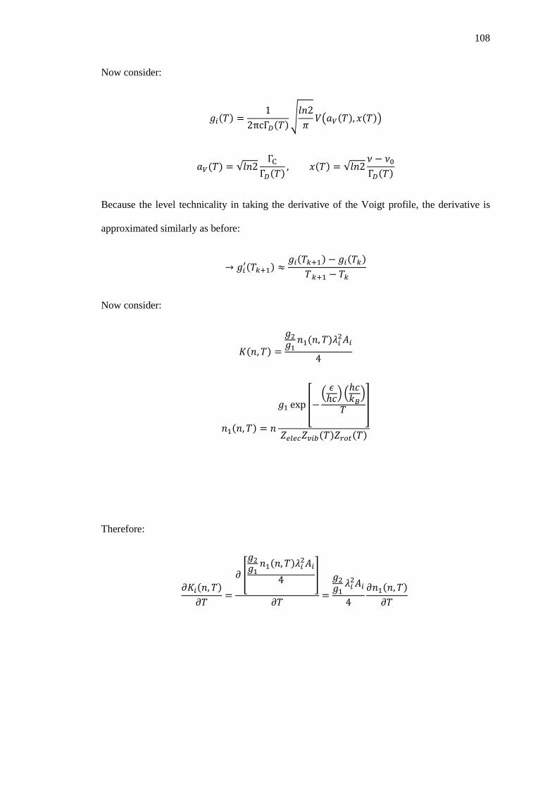
108
Now consider:
𝑔𝑔𝑖𝑖(𝑇𝑇) =1
2πcΓ𝐷𝐷(𝑇𝑇)�𝑔𝑔𝑛𝑛2𝜋𝜋𝑃𝑃�𝑎𝑎𝑉𝑉(𝑇𝑇),𝑥𝑥(𝑇𝑇)�
𝑎𝑎𝑉𝑉(𝑇𝑇) = √𝑔𝑔𝑛𝑛2ΓC
Γ𝐷𝐷(𝑇𝑇) , 𝑥𝑥(𝑇𝑇) = √𝑔𝑔𝑛𝑛2𝜈𝜈 − 𝜈𝜈0Γ𝐷𝐷(𝑇𝑇)
Because the level technicality in taking the derivative of the Voigt profile, the derivative is
approximated similarly as before:
→ 𝑔𝑔𝑖𝑖′(𝑇𝑇𝑖𝑖+1) ≈𝑔𝑔𝑖𝑖(𝑇𝑇𝑖𝑖+1) − 𝑔𝑔𝑖𝑖(𝑇𝑇𝑖𝑖)
𝑇𝑇 𝑖𝑖+1 − 𝑇𝑇𝑖𝑖
Now consider:
𝐾𝐾(𝑛𝑛,𝑇𝑇) =
𝑔𝑔2𝑔𝑔1𝑛𝑛1(𝑛𝑛,𝑇𝑇)𝜆𝜆𝑖𝑖2𝐴𝐴𝑖𝑖
4
𝑛𝑛1(𝑛𝑛,𝑇𝑇) = 𝑛𝑛
𝑔𝑔1 exp �−� 𝜖𝜖ℎ𝑔𝑔� �
ℎ𝑔𝑔𝑘𝑘𝐵𝐵�
𝑇𝑇 �
𝑍𝑍𝑒𝑒𝑏𝑏𝑒𝑒𝑐𝑐𝑍𝑍𝑣𝑣𝑖𝑖𝑏𝑏(𝑇𝑇)𝑍𝑍𝑟𝑟𝑡𝑡𝑡𝑡(𝑇𝑇)
Therefore:
𝜕𝜕𝐾𝐾𝑖𝑖(𝑛𝑛,𝑇𝑇)𝜕𝜕𝑇𝑇
=
𝜕𝜕 �
𝑔𝑔2𝑔𝑔1𝑛𝑛1(𝑛𝑛,𝑇𝑇)𝜆𝜆𝑖𝑖2𝐴𝐴𝑖𝑖
4 �
𝜕𝜕𝑇𝑇=
𝑔𝑔2𝑔𝑔1𝜆𝜆𝑖𝑖2𝐴𝐴𝑖𝑖4
𝜕𝜕𝑛𝑛1(𝑛𝑛,𝑇𝑇)𝜕𝜕𝑇𝑇

109
For CH an OH population densities the following parameters were kept constant:
o z
o Γ𝐶𝐶
o 𝑛𝑛
Property Combinations
If the model shows a higher sensitivity to more than one parameter then another analysis
whereby the sensitivity of the model to the parameters simultaneously must be investigated.
One such approach is to investigate the variation in the sensitivity of the absorption with respect
to one parameter with respect to another.
It is possible that the model may be much more sensitive to the perturbation of more than
parameter at a time and must be investigated to insure the model’s stability for all parameters.
3.4.3 Error Estimates
The propagation of uncertainty in calculations is of main concern when trying to verify the
accuracy and precision of a model. The uncertainty in constant values may be negligible when
they are isolated in an exact equation, however, when many values, each with their own levels
of uncertainty, are operated together then the error or uncertainty may blow up to significant
levels in the final output.
The uncertainty of a value or dataset can be described using numerous methods, such as:
variance, standard deviation, relative error, etc., depending on the error model used. For the
purpose of this error propagation investigation the uncertainty will be described using the
standard deviation of a Gaussian distribution associated with the statistical variation in the
value. The error can propagate in the following ways [54], shown in below:

110
Table 12: Propagation of Error in Computations.
Type Example Standard Deviation (𝝈𝝈𝒙𝒙)
Linear Operation 𝑥𝑥 = 𝑎𝑎 + 𝑏𝑏 − 𝑔𝑔 𝜎𝜎𝑚𝑚 = �𝜎𝜎𝑎𝑎2 + 𝜎𝜎𝑏𝑏2 + 𝜎𝜎𝑐𝑐2
Product or Quotient Operation 𝑥𝑥 = 𝑎𝑎 ×
𝑏𝑏𝑔𝑔
𝜎𝜎𝑚𝑚𝑥𝑥
= ��𝜎𝜎𝑎𝑎𝑎𝑎�2
+ �𝜎𝜎𝑏𝑏𝑏𝑏�2
+ �𝜎𝜎𝑐𝑐𝑔𝑔�2
Exponent 𝑥𝑥 = 𝑎𝑎𝑑𝑑 𝜎𝜎𝑚𝑚𝑥𝑥
= 𝑦𝑦 �𝜎𝜎𝑎𝑎𝑎𝑎�
Exponential 𝑥𝑥 = 𝑒𝑒𝑥𝑥𝑝𝑝(𝑎𝑎𝑦𝑦) 𝜎𝜎𝑚𝑚 ≈ |𝑥𝑥(𝑦𝑦𝜎𝜎𝑎𝑎)|
Logarithmic 𝑥𝑥 = ln (𝑎𝑎) 𝜎𝜎𝑚𝑚 = 0.434 �𝜎𝜎𝑎𝑎𝑎𝑎�
The variance of a dataset can be calculated by:
𝜎𝜎 = �∑(𝑥𝑥𝑖𝑖 − �̅�𝑥)2
𝑁𝑁 − 1
(120)
The standard deviation is calculated as the square root of the summation of the distance between
each data point value 𝑥𝑥𝑖𝑖 from the dataset mean �̅�𝑥 for 𝑁𝑁 data points. For the purpose of
verification of the model it may be necessary to scrutinize every major section of code and
consider the accuracy of each numerical computation.

111
4. VERIFICATION DATA
This section displays the data with the purpose of verifying the optical model. The effects of
line broadening, a sensitivity study for various model parameters and an error estimation of the
model are all investigated in this section.
4.1 Effect of Line Broadening on Signal Strength
To visualize the effect that line broadening has on absorption Figure 65 and Figure 66 were
created using one of the main high strength transitions in the OH* and CH* bands. Specifically,
the 𝑃𝑃1(1.5) of OH and 𝑅𝑅1𝑎𝑎 + 𝑅𝑅1𝑏𝑏(1.5) of CH were used. The effects show the reduction of the
line strength of absorption at a specific wavelength due to line broadening.

112
Figure 65: Monochromatic and Broadened Absorption Lines for 𝑃𝑃1(1.5) Transition of OH for a Number Density of 1021 𝑔𝑔−3 and a Temperature of 2500K.
Figure 66: Monochromatic and Broadened Absorption Lines for 𝑅𝑅1𝑎𝑎 + 𝑅𝑅1𝑏𝑏 (1.5) Transition of CH for a Number Density of 1021 𝑔𝑔−3 and a Temperature of 2500K.
113
4.2 Sensitivity Study
The model sensitivity to parameters pertinent to the calculation of absorption effects are
detailed in this section. The main parameters of importance are number density, optical path
length, collisional linewidth and Doppler linewidth, which is related to temperature. Using the
equations derived in the previous section these parameters are varied and the relative sensitivity
of the model’s prediction of the effect of absorption is monitored. Unless otherwise stated the
sensitivity study is performed with the following parameters corresponding approximately to
the conditions during combustion within the CVRC:
o T = 2500K
o z = 0.045m
o Γ𝑐𝑐 = 0.5𝑔𝑔𝑔𝑔−1
4.2.1 Transmissivity with Respect to Number Density
The normalized transmissivity of the combustion medium with respect to the ground state
number densities of the OH and CH radicals for different optical path lengths are displayed
below in Figure 67 and Figure 68. The charts are based on the sensitivity analysis from Equation
116.

114
Figure 67: Normalized Sensitivity of Transmissivity to Variation of the OH Ground State Number Density for different Optical Path Lengths
.
Figure 68: Normalized Sensitivity of Transmissivity to Variation of the CH Ground State Number Density for different Optical Path Lengths.

115
From Equation 87 it can be shown that the transmissivity is related to the ground state number
density and optical path length by:
ln �1𝜏𝜏� ∝ 𝑁𝑁, 𝑧𝑧
(121)
Equation 121 represents the strongest dependency of the transmissivity with respect to the
parameters of interest. For an optical path length of z = 0.045m, which is equivalent to the width
of the CVRC chamber, it is clear from Figure 67 that the combustion medium is optically thin
for emissions from CH*, for a ground state number density of approximately 5 × 10¹⁹𝑔𝑔−3 or
less. The opposite occurs (full absorption, optically thick) when the ground state number
density is approximately greater or equal to 1022𝑔𝑔−3. Similarly for OH, which does not have
a significantly different spectrum with respect to other molecules, the combustion medium is
optically thin for ground state number densities less than or equal to 1020𝑔𝑔−3 and optically
thick for ground state number densities greater than or equal to 1022𝑔𝑔−3. To illustrate the
sensitivity of the absorption more clearly for this specific optical path length a comparison of
the absorption of OH* and CH* for varying number density is shown in Figure 69.

116
Figure 69: Absorption Sensitivity to Variations of Ground State Number Density of OH and CH for an Optical Path Length of z = 0.045m.
The data from Figure 69 show that the absorption is most sensitive, for an optical path length
of z = 0.045m, between the ranges of approximately 1018 and 1022𝑔𝑔−3. Thus, the investigation
of the rest of the parameters will be conducted with reference to the ranges of these number
densities.
4.2.2 Sensitivity to Optical Path Length
In this section the sensitivity of the absorption to optical depth and number density are
investigated. Using Equation 117 the sensitivity to the perturbation in the aforementioned
parameters with respect to OH and CH are shown in Figure 70 and Figure 71 respectively.

117
Figure 70: Variation in Absorption Sensitivity with Perturbations in the Optical Depth with Varying Number Densities of OH.
Figure 71: Variation in Absorption Sensitivity with Perturbations in the Optical Depth with Varying Number Densities of CH.
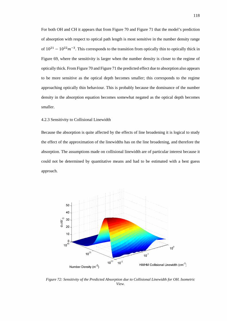
118
For both OH and CH it appears that from Figure 70 and Figure 71 that the model’s prediction
of absorption with respect to optical path length is most sensitive in the number density range
of 1021 − 1022𝑔𝑔−3. This corresponds to the transition from optically thin to optically thick in
Figure 69, where the sensitivity is larger when the number density is closer to the regime of
optically thick. From Figure 70 and Figure 71 the predicted effect due to absorption also appears
to be more sensitive as the optical depth becomes smaller; this corresponds to the regime
approaching optically thin behaviour. This is probably because the dominance of the number
density in the absorption equation becomes somewhat negated as the optical depth becomes
smaller.
4.2.3 Sensitivity to Collisional Linewidth
Because the absorption is quite affected by the effects of line broadening it is logical to study
the effect of the approximation of the linewidths has on the line broadening, and therefore the
absorption. The assumptions made on collisional linewidth are of particular interest because it
could not be determined by quantitative means and had to be estimated with a best guess
approach.
Figure 72: Sensitivity of the Predicted Absorption due to Collisional Linewidth for OH. Isometric View.

119
Figure 73: Sensitivity of the Predicted Absorption due to Collisional Linewidth for OH. Top View
.
Figure 74: Sensitivity of the Predicted Absorption due to Collisional Linewidth for CH. Isometric View.

120
Figure 75: Sensitivity of the Predicted Absorption due to Collisional Linewidth for CH. Top View.
As with the previous sensitivity studies Figure 72 and Figure 73 for OH, and Figure 74 and
Figure 75 for CH show the maximum region of sensitivity to be within the same number density
range as before. Comparing the collisional broadening sensitivity data with that of optical path
length and number density it appears that the predicted absorption is relatively less sensitive
than for the case of perturbations in number density and optical path length. Also, as expected,
the sensitivity of absorption due to collisional linewidth becomes much greater as the linewidth
becomes shorter; a shorter linewidth results in stronger absorption effects on the incident
radiation. At and near the location where it has been assumed that the linewidth is 0.5𝑔𝑔𝑔𝑔−1
(HWHM) the sensitivity to absorption for both OH and CH is relatively much lower than for
optical path length and number density. Thus, it can be assumed, with a fair amount of
confidence, that the collisional linewidth will not affect the absorption results significantly in
comparison to other parameters.
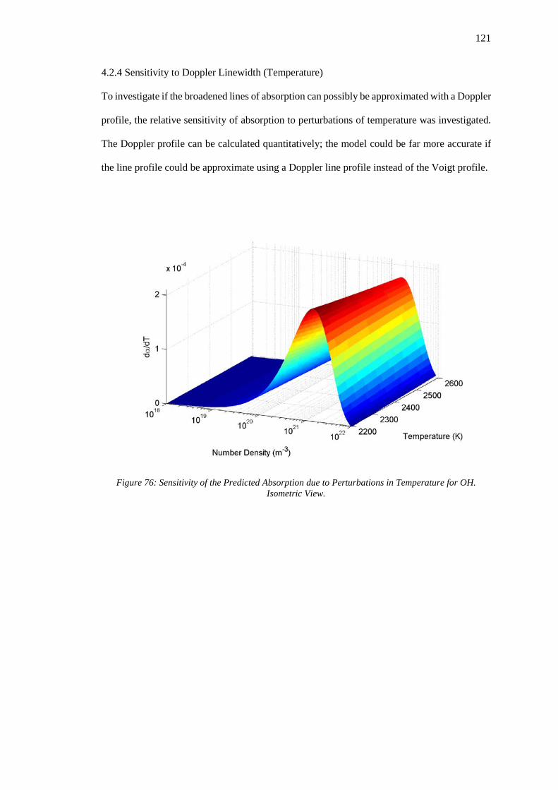
121
4.2.4 Sensitivity to Doppler Linewidth (Temperature)
To investigate if the broadened lines of absorption can possibly be approximated with a Doppler
profile, the relative sensitivity of absorption to perturbations of temperature was investigated.
The Doppler profile can be calculated quantitatively; the model could be far more accurate if
the line profile could be approximate using a Doppler line profile instead of the Voigt profile.
Figure 76: Sensitivity of the Predicted Absorption due to Perturbations in Temperature for OH. Isometric View.

122
Figure 77: Sensitivity of the Predicted Absorption due to Perturbations in Temperature for OH. Top View.
Figure 78: Sensitivity of the Predicted Absorption due to Perturbations in Temperature for CH. Isometric View.
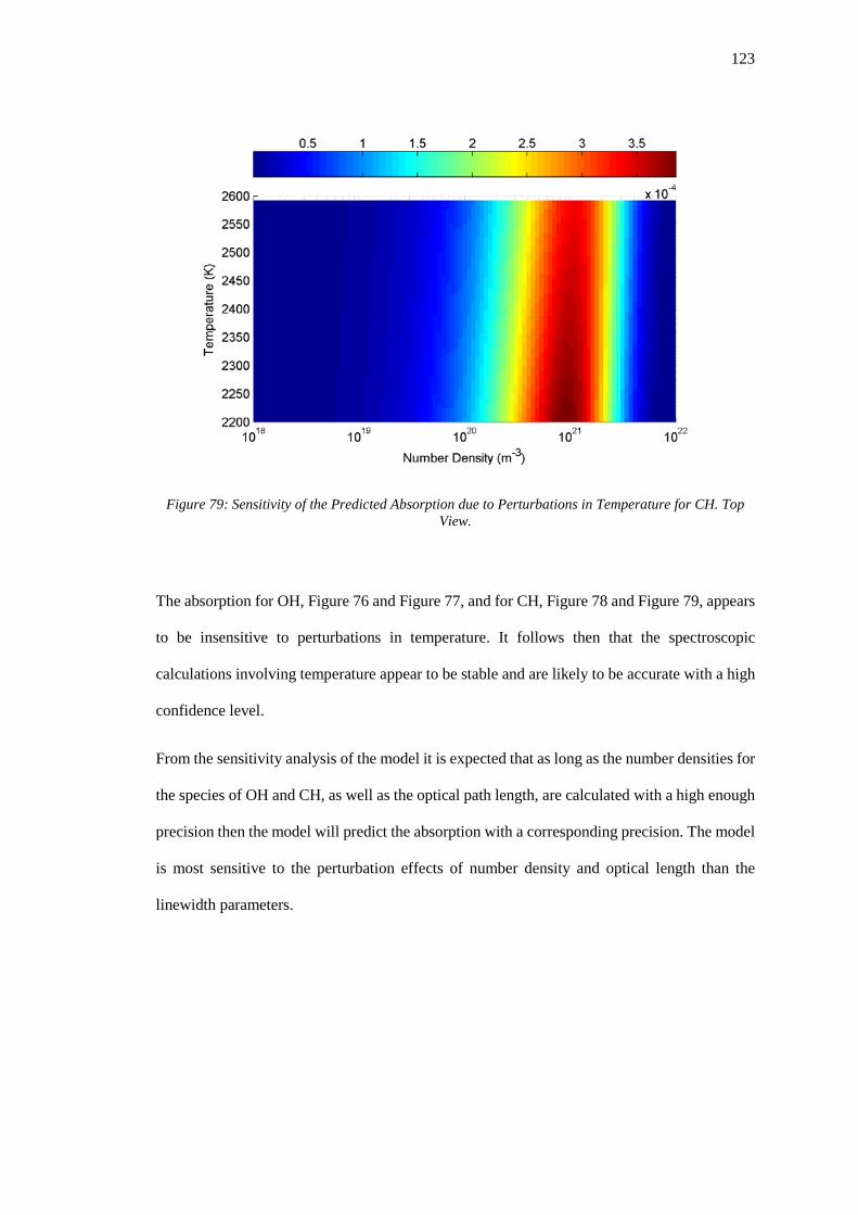
123
Figure 79: Sensitivity of the Predicted Absorption due to Perturbations in Temperature for CH. Top View.
The absorption for OH, Figure 76 and Figure 77, and for CH, Figure 78 and Figure 79, appears
to be insensitive to perturbations in temperature. It follows then that the spectroscopic
calculations involving temperature appear to be stable and are likely to be accurate with a high
confidence level.
From the sensitivity analysis of the model it is expected that as long as the number densities for
the species of OH and CH, as well as the optical path length, are calculated with a high enough
precision then the model will predict the absorption with a corresponding precision. The model
is most sensitive to the perturbation effects of number density and optical length than the
linewidth parameters.

124
4.3 Error Estimation
The approximate error of the model can be estimate using the propagation of uncertainty or
standard deviation using Table 12. The maximum standard deviation of the data of the CFD
model is estimated with the variable 𝜎𝜎𝐸𝐸. The approach is to directly infer the error propagation
from the method of calculating the spectra in the model.
4.3.1 Data Initialisation from CFD
The initial data from the CFD is extracted and averaged per each cell of the probe volume
within the model. The number density per shell in the model is calculated in the following way:
𝑁𝑁 = ��(𝑌𝑌𝜌𝜌) ×1000𝑁𝑁𝐴𝐴ℳ � ×
𝑃𝑃𝑟𝑟ℎ𝑒𝑒𝑏𝑏𝑏𝑏𝑃𝑃𝑡𝑡𝑡𝑡𝑡𝑡
, where 𝑌𝑌 is the mass fraction, 𝜌𝜌 is the density, 𝑁𝑁𝑚𝑚𝑡𝑡𝑏𝑏 is Avogadro’s constant, and 𝑃𝑃 is the
volume. The variance of the summation of the mass fraction multiplied by the density for a
given shell is given by:
𝜎𝜎𝜒𝜒𝑟𝑟ℎ = �𝑛𝑛𝑝𝑝𝑟𝑟𝜎𝜎𝐸𝐸2 = �𝑛𝑛𝑝𝑝𝑟𝑟𝜎𝜎𝐸𝐸
(122)
, where the number of discrete points in that shell is given by 𝑛𝑛𝑝𝑝𝑟𝑟. In general the standard
deviation of the number density for the shell can then be expressed as:
𝜎𝜎𝑁𝑁 = 𝑁𝑁𝑟𝑟ℎ𝑒𝑒𝑏𝑏𝑏𝑏�𝑛𝑛𝑝𝑝𝑟𝑟 �
𝜎𝜎𝐸𝐸𝜒𝜒𝑟𝑟ℎ
�2
+ �𝜎𝜎ℳℳ
�2
+ �𝜎𝜎𝑁𝑁𝐴𝐴𝑁𝑁𝐴𝐴
�2
+ �𝜎𝜎𝑣𝑣𝑃𝑃𝑡𝑡𝑡𝑡𝑡𝑡
�2
+ �𝜎𝜎𝑣𝑣𝑟𝑟ℎ𝑒𝑒𝑏𝑏𝑏𝑏𝑃𝑃𝑟𝑟ℎ𝑒𝑒𝑏𝑏𝑏𝑏
�2
(123)
Now since, 𝑃𝑃𝑟𝑟ℎ𝑒𝑒𝑏𝑏𝑏𝑏 = 𝑛𝑛𝑝𝑝𝑝𝑝𝑛𝑛𝑝𝑝𝑝𝑝𝑝𝑝𝑝𝑝
𝑃𝑃𝑡𝑡𝑡𝑡𝑡𝑡, where 𝑛𝑛𝑝𝑝𝑡𝑡𝑡𝑡𝑡𝑡 is the number of discrete points within the whole
probe volume. Therefore Equation 123 becomes:
𝜎𝜎𝑁𝑁 = 𝑁𝑁𝑟𝑟ℎ𝑒𝑒𝑏𝑏𝑏𝑏�𝑛𝑛𝑝𝑝𝑟𝑟 �
𝜎𝜎𝐸𝐸𝜒𝜒𝑟𝑟ℎ𝑒𝑒𝑏𝑏𝑏𝑏
�2
+ �𝜎𝜎ℳℳ
�2
+ �𝜎𝜎𝐸𝐸𝑁𝑁𝐴𝐴�2
+ �𝜎𝜎𝑣𝑣𝑃𝑃𝑡𝑡𝑡𝑡𝑡𝑡
�2
+ �𝑛𝑛𝑝𝑝𝑡𝑡𝑡𝑡𝑡𝑡𝜎𝜎𝑣𝑣𝑟𝑟ℎ𝑒𝑒𝑏𝑏𝑏𝑏𝑛𝑛𝑝𝑝𝑟𝑟𝑃𝑃𝑡𝑡𝑡𝑡𝑡𝑡
�2
(124)

125
The temperature per probe volume is calculated in the model by:
𝑇𝑇𝑟𝑟ℎ𝑒𝑒𝑏𝑏𝑏𝑏 = �𝑇𝑇 ×𝑃𝑃𝑟𝑟ℎ𝑒𝑒𝑏𝑏𝑏𝑏𝑃𝑃𝑡𝑡𝑡𝑡𝑡𝑡
Using Equation 122 the standard deviation of the temperature per shell is calculated by:
𝜎𝜎𝑇𝑇 = 𝑇𝑇𝑟𝑟ℎ𝑒𝑒𝑏𝑏𝑏𝑏�𝑛𝑛𝑝𝑝𝑟𝑟 �
𝜎𝜎𝐸𝐸𝑇𝑇𝑟𝑟ℎ𝑒𝑒𝑏𝑏𝑏𝑏
�2
+ �𝜎𝜎𝑣𝑣𝑃𝑃𝑡𝑡𝑡𝑡𝑡𝑡
�2
+ �𝑛𝑛𝑝𝑝𝑡𝑡𝑡𝑡𝑡𝑡𝜎𝜎𝑣𝑣𝑟𝑟ℎ𝑒𝑒𝑏𝑏𝑏𝑏𝑛𝑛𝑝𝑝𝑟𝑟𝑃𝑃𝑡𝑡𝑡𝑡𝑡𝑡
�2
(125)
The same procedure applies to calculating the pressure.
4.3.2 Uncorrected Emission
The emission per shell is calculated in the model by:
𝐼𝐼 =ℎ𝑔𝑔𝜆𝜆
× 𝑛𝑛1
, where 𝑛𝑛1 is the number density per state distributed according to the Maxwell-Boltzmann
distribution. The partition function is calculated using:
𝑛𝑛1 =𝑁𝑁𝑔𝑔1 exp �− 𝐸𝐸
ℎ𝑔𝑔 × ℎ𝑔𝑔𝑘𝑘𝐵𝐵𝑇𝑇
�
𝑍𝑍𝑒𝑒𝑏𝑏𝑒𝑒𝑐𝑐𝑍𝑍𝑟𝑟𝑡𝑡𝑡𝑡𝑍𝑍𝑣𝑣𝑖𝑖𝑏𝑏
The partition function follows Equation 100 and the relevant corresponding sub equations. The
standard deviation per sub equation will be calculated in pieces before connecting them
together. The partition function for the electronic transitions is exact. The standard deviation
for the other partition functions are:
For rotation:
𝑍𝑍𝑟𝑟𝑡𝑡𝑡𝑡 =𝑇𝑇𝑐𝑐𝑟𝑟𝑡𝑡𝑡𝑡
𝑐𝑐𝑟𝑟𝑡𝑡𝑡𝑡 =ℎ𝑔𝑔𝑘𝑘𝐵𝐵
× 𝐵𝐵∗
𝜎𝜎𝜃𝜃𝑟𝑟𝑝𝑝𝑝𝑝 = 𝑐𝑐𝑟𝑟𝑡𝑡𝑡𝑡��
𝜎𝜎ℎℎ�2
+ �𝜎𝜎𝑖𝑖𝐵𝐵𝑘𝑘𝐵𝐵
�2
(126)
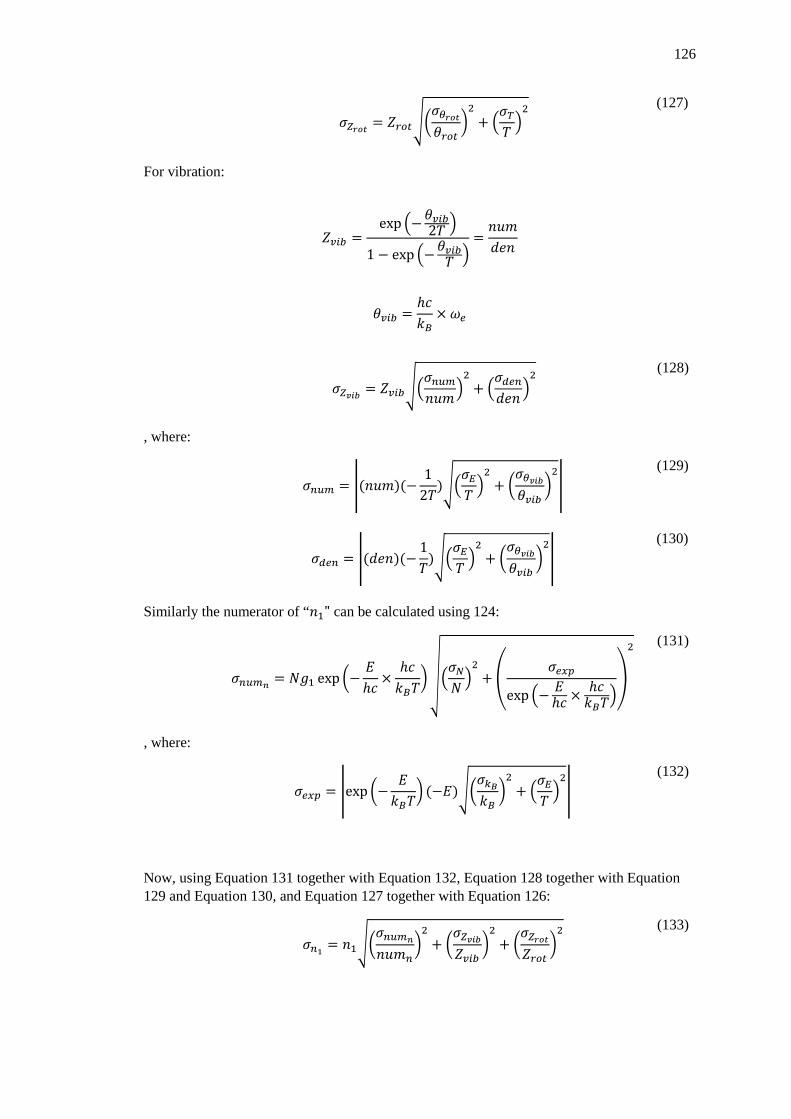
126
𝜎𝜎𝑍𝑍𝑟𝑟𝑝𝑝𝑝𝑝 = 𝑍𝑍𝑟𝑟𝑡𝑡𝑡𝑡��
𝜎𝜎𝜃𝜃𝑟𝑟𝑝𝑝𝑝𝑝𝑐𝑐𝑟𝑟𝑡𝑡𝑡𝑡
�2
+ �𝜎𝜎𝑇𝑇𝑇𝑇�2
(127)
For vibration:
𝑍𝑍𝑣𝑣𝑖𝑖𝑏𝑏 =exp �−𝑐𝑐𝑣𝑣𝑖𝑖𝑏𝑏2𝑇𝑇 �
1 − exp �−𝑐𝑐𝑣𝑣𝑖𝑖𝑏𝑏𝑇𝑇 �=𝑛𝑛𝐹𝐹𝑔𝑔𝑑𝑑𝑒𝑒𝑛𝑛
𝑐𝑐𝑣𝑣𝑖𝑖𝑏𝑏 =ℎ𝑔𝑔𝑘𝑘𝐵𝐵
× 𝜔𝜔𝑒𝑒
𝜎𝜎𝑍𝑍𝑣𝑣𝑖𝑖𝑣𝑣 = 𝑍𝑍𝑣𝑣𝑖𝑖𝑏𝑏��
𝜎𝜎𝑛𝑛𝑢𝑢𝑚𝑚𝑛𝑛𝐹𝐹𝑔𝑔
�2
+ �𝜎𝜎𝑑𝑑𝑒𝑒𝑛𝑛𝑑𝑑𝑒𝑒𝑛𝑛
�2
(128)
, where:
𝜎𝜎𝑛𝑛𝑢𝑢𝑚𝑚 = �(𝑛𝑛𝐹𝐹𝑔𝑔)(−
12𝑇𝑇
)��𝜎𝜎𝐸𝐸𝑇𝑇�2
+ �𝜎𝜎𝜃𝜃𝑣𝑣𝑖𝑖𝑣𝑣𝑐𝑐𝑣𝑣𝑖𝑖𝑏𝑏
�2�
(129)
𝜎𝜎𝑑𝑑𝑒𝑒𝑛𝑛 = �(𝑑𝑑𝑒𝑒𝑛𝑛)(−
1𝑇𝑇
)��𝜎𝜎𝐸𝐸𝑇𝑇�2
+ �𝜎𝜎𝜃𝜃𝑣𝑣𝑖𝑖𝑣𝑣𝑐𝑐𝑣𝑣𝑖𝑖𝑏𝑏
�2�
(130)
Similarly the numerator of “𝑛𝑛1" can be calculated using 124:
𝜎𝜎𝑛𝑛𝑢𝑢𝑚𝑚𝑛𝑛 = 𝑁𝑁𝑔𝑔1 exp �−𝐸𝐸ℎ𝑔𝑔
×ℎ𝑔𝑔𝑘𝑘𝐵𝐵𝑇𝑇
���𝜎𝜎𝑁𝑁𝑁𝑁�2
+ �𝜎𝜎𝑒𝑒𝑚𝑚𝑝𝑝
exp �− 𝐸𝐸ℎ𝑔𝑔 × ℎ𝑔𝑔
𝑘𝑘𝐵𝐵𝑇𝑇��
2
(131)
, where:
𝜎𝜎𝑒𝑒𝑚𝑚𝑝𝑝 = �exp �−
𝐸𝐸𝑘𝑘𝐵𝐵𝑇𝑇
� (−𝐸𝐸)��𝜎𝜎𝑖𝑖𝐵𝐵𝑘𝑘𝐵𝐵
�2
+ �𝜎𝜎𝐸𝐸𝑇𝑇�2�
(132)
Now, using Equation 131 together with Equation 132, Equation 128 together with Equation 129 and Equation 130, and Equation 127 together with Equation 126:
𝜎𝜎𝑛𝑛1 = 𝑛𝑛1��
𝜎𝜎𝑛𝑛𝑢𝑢𝑚𝑚𝑛𝑛
𝑛𝑛𝐹𝐹𝑔𝑔𝑛𝑛�2
+ �𝜎𝜎𝑍𝑍𝑣𝑣𝑖𝑖𝑣𝑣𝑍𝑍𝑣𝑣𝑖𝑖𝑏𝑏
�2
+ �𝜎𝜎𝑍𝑍𝑟𝑟𝑝𝑝𝑝𝑝𝑍𝑍𝑟𝑟𝑡𝑡𝑡𝑡
�2
(133)

127
Then the standard deviation of the resulting emission per shell, using Equation 133, is given by:
𝜎𝜎𝐼𝐼 = 𝐼𝐼��
𝜎𝜎ℎℎ�2
+ �𝜎𝜎𝑛𝑛1𝑛𝑛1�2
(134)
Now from Equation 134 with the correction due to solid angle and volume the standard deviation of the resulting emission per shell is given by:
𝜎𝜎𝐼𝐼𝑒𝑒𝑒𝑒 = 𝐼𝐼𝑒𝑒𝑚𝑚��
𝜎𝜎𝐼𝐼𝐼𝐼�2
+ �𝜎𝜎𝑣𝑣𝑃𝑃𝑡𝑡𝑡𝑡𝑡𝑡
�2
(135)
The standard deviation of the resultant probe volume emission is:
𝜎𝜎𝑅𝑅𝑒𝑒𝑟𝑟𝐸𝐸𝑚𝑚 = �𝜎𝜎𝐼𝐼𝑒𝑒𝑒𝑒(1)
2 + 𝜎𝜎𝐼𝐼𝑒𝑒𝑒𝑒(2)2 +⋯+ 𝜎𝜎𝐼𝐼𝑒𝑒𝑒𝑒(𝑛𝑛𝑝𝑝ℎ)
2 (136)
, where 𝑛𝑛𝑟𝑟ℎ is the number of shells.
4.3.3 Resultant Emission and Absorption
For the calculation of absorption by the model, the transmissivity and line strength is calculated
with:
𝜏𝜏 = exp(−𝐾𝐾 ∗ 𝑔𝑔 ∗ 𝑧𝑧) = exp (−𝐵𝐵′ ∗ 𝑧𝑧)
𝐾𝐾 =
𝑛𝑛1𝑔𝑔2𝑔𝑔1
𝜆𝜆2𝐴𝐴214
The standard deviation of the line strength is calculated, with Equation 133 by:
𝜎𝜎𝐾𝐾 = 𝐾𝐾��
𝜎𝜎𝑛𝑛1𝑛𝑛1�2
+ �𝜎𝜎𝐴𝐴21𝐴𝐴21
�2
(137)
The Voigt line profile is calculate with a polynomial expression with the use of linewidths; the
collisional linewidth is approximated and therefore has no standard deviation; there is an error
associated with it, but it cannot be quantified. The standard deviation of the Voigt line profile
is calculated by:

128
𝜎𝜎𝑣𝑣𝑡𝑡𝑖𝑖𝑔𝑔𝑡𝑡 = 𝑦𝑦𝑣𝑣𝑡𝑡𝑖𝑖𝑔𝑔𝑡𝑡�2 �
𝜎𝜎ΓDΓD
�2
(138)
, where 𝑦𝑦𝑣𝑣𝑡𝑡𝑖𝑖𝑔𝑔𝑡𝑡 are the values of the Voigt profile and ΓD is the Doppler linewidth:
Γ𝐷𝐷 = 𝜈𝜈𝑝𝑝𝑎𝑎𝑡𝑡�2𝑔𝑔𝑛𝑛(2)𝑘𝑘𝐵𝐵𝑇𝑇𝑔𝑔𝑎𝑎𝑔𝑔2
= 𝜈𝜈𝑝𝑝𝑎𝑎𝑡𝑡√𝑎𝑎
The corresponding standard deviation is:
𝜎𝜎Γ𝐷𝐷 =
Γ𝐷𝐷2�𝜎𝜎𝑎𝑎𝑎𝑎
(139)
𝜎𝜎𝑎𝑎 = 𝑎𝑎��
𝜎𝜎𝑖𝑖𝐵𝐵𝑘𝑘𝐵𝐵
�2
+ �𝜎𝜎𝑇𝑇𝑇𝑇�2
+ �𝜎𝜎ℳℳ
�2
(140)
Now the standard deviation for the transmissivity:
𝜎𝜎𝐵𝐵′ = 𝐾𝐾𝑔𝑔��
𝜎𝜎𝐾𝐾𝐾𝐾�2
+ �𝜎𝜎𝑣𝑣𝑡𝑡𝑖𝑖𝑔𝑔𝑡𝑡𝑦𝑦𝑣𝑣𝑡𝑡𝑖𝑖𝑔𝑔𝑡𝑡
�2
(141)
𝜎𝜎𝜏𝜏 ≈ |exp(−𝐾𝐾𝑔𝑔𝑧𝑧)(−𝑧𝑧)𝜎𝜎𝐵𝐵′| (142)
Therefore the standard deviation of the resulting emission from each shell:
𝑅𝑅𝑒𝑒𝑠𝑠𝜏𝜏 = �𝜏𝜏𝑖𝑖
𝑛𝑛𝑝𝑝
𝑖𝑖=1
𝜎𝜎𝑅𝑅𝑒𝑒𝑟𝑟𝜏𝜏 = 𝑅𝑅𝑒𝑒𝑠𝑠𝜏𝜏��
𝜎𝜎𝜏𝜏𝑟𝑟ℎ𝑒𝑒𝑏𝑏𝑏𝑏1𝜏𝜏𝑠𝑠ℎ𝑒𝑒𝑔𝑔𝑔𝑔1
�2
+ �𝜎𝜎𝜏𝜏𝑟𝑟ℎ𝑒𝑒𝑏𝑏𝑏𝑏2𝜏𝜏𝑠𝑠ℎ𝑒𝑒𝑔𝑔𝑔𝑔2
�2
+ ⋯+ �𝜎𝜎𝜏𝜏𝑟𝑟ℎ𝑒𝑒𝑏𝑏𝑏𝑏𝑛𝑛𝑝𝑝𝜏𝜏𝑠𝑠ℎ𝑒𝑒𝑔𝑔𝑔𝑔𝑛𝑛𝑝𝑝
�2
(143)
, where 𝑛𝑛𝑟𝑟 is the number of shells from the measurement point to the emission point,
𝜎𝜎𝑅𝑅𝑒𝑒𝑟𝑟𝐸𝐸𝑚𝑚𝑅𝑅ℎ𝑒𝑒𝑏𝑏𝑏𝑏 = 𝐼𝐼𝑅𝑅𝑒𝑒𝑟𝑟𝐸𝐸𝑚𝑚𝐴𝐴𝑏𝑏𝑟𝑟��
𝜎𝜎𝐼𝐼𝑒𝑒𝑒𝑒𝐼𝐼𝑒𝑒𝑚𝑚
�2
+ �𝜎𝜎𝑅𝑅𝑒𝑒𝑟𝑟𝜏𝜏𝑅𝑅𝑒𝑒𝑠𝑠𝜏𝜏
�2
(144)
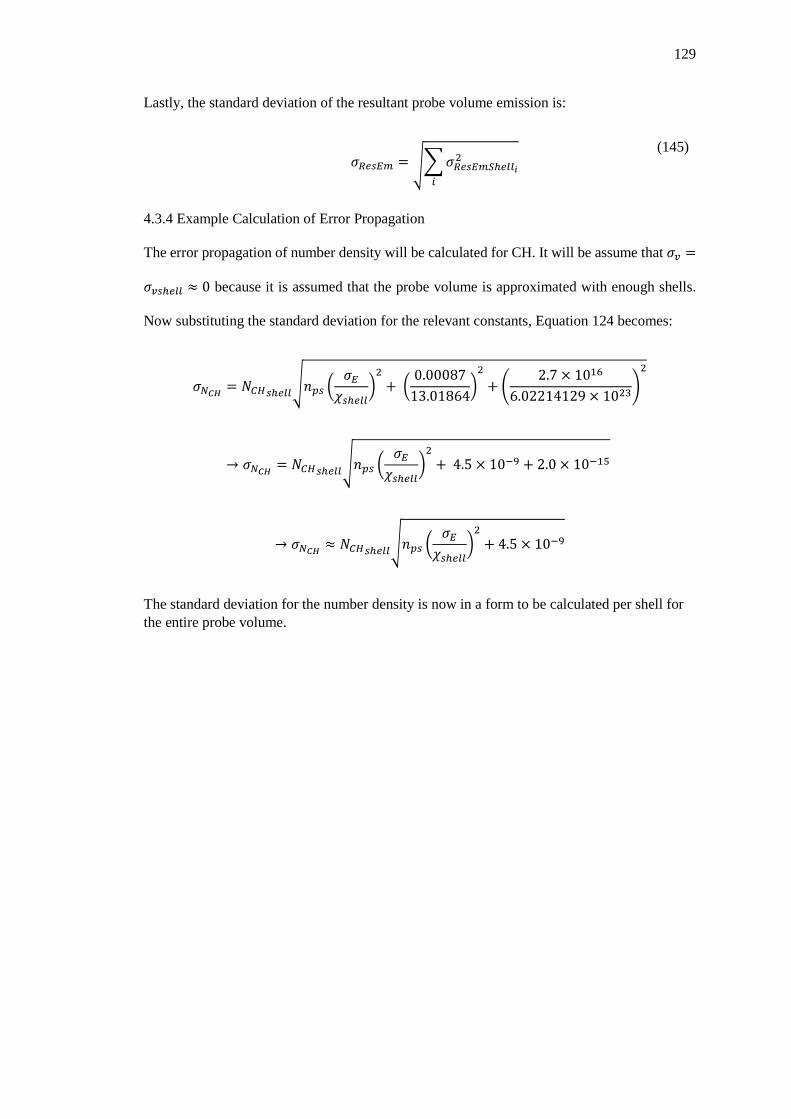
129
Lastly, the standard deviation of the resultant probe volume emission is:
𝜎𝜎𝑅𝑅𝑒𝑒𝑟𝑟𝐸𝐸𝑚𝑚 = ��𝜎𝜎𝑅𝑅𝑒𝑒𝑟𝑟𝐸𝐸𝑚𝑚𝑅𝑅ℎ𝑒𝑒𝑏𝑏𝑏𝑏𝑖𝑖
2
𝑖𝑖
(145)
4.3.4 Example Calculation of Error Propagation
The error propagation of number density will be calculated for CH. It will be assume that 𝜎𝜎𝑣𝑣 =
𝜎𝜎𝑣𝑣𝑟𝑟ℎ𝑒𝑒𝑏𝑏𝑏𝑏 ≈ 0 because it is assumed that the probe volume is approximated with enough shells.
Now substituting the standard deviation for the relevant constants, Equation 124 becomes:
𝜎𝜎𝑁𝑁𝐶𝐶𝐶𝐶 = 𝑁𝑁𝐶𝐶𝐻𝐻𝑟𝑟ℎ𝑒𝑒𝑏𝑏𝑏𝑏�𝑛𝑛𝑝𝑝𝑟𝑟 �𝜎𝜎𝐸𝐸
𝜒𝜒𝑟𝑟ℎ𝑒𝑒𝑏𝑏𝑏𝑏�2
+ �0.00087
13.01864�2
+ �2.7 × 10¹⁶
6.02214129 × 10²³�2
→ 𝜎𝜎𝑁𝑁𝐶𝐶𝐶𝐶 = 𝑁𝑁𝐶𝐶𝐻𝐻𝑟𝑟ℎ𝑒𝑒𝑏𝑏𝑏𝑏�𝑛𝑛𝑝𝑝𝑟𝑟 �𝜎𝜎𝐸𝐸
𝜒𝜒𝑟𝑟ℎ𝑒𝑒𝑏𝑏𝑏𝑏�2
+ 4.5 × 10⁻⁹ + 2.0 × 10⁻¹⁵
→ 𝜎𝜎𝑁𝑁𝐶𝐶𝐶𝐶 ≈ 𝑁𝑁𝐶𝐶𝐻𝐻𝑟𝑟ℎ𝑒𝑒𝑏𝑏𝑏𝑏�𝑛𝑛𝑝𝑝𝑟𝑟 �𝜎𝜎𝐸𝐸
𝜒𝜒𝑟𝑟ℎ𝑒𝑒𝑏𝑏𝑏𝑏�2
+ 4.5 × 10⁻⁹
The standard deviation for the number density is now in a form to be calculated per shell for the entire probe volume.

130
5. RESULTS
The spectral data and results pertaining to the CVRC experiment are detailed within this
section. The data are derived from the CVRC computational model. The calculated spectral
output is displayed for the span of one oscillation cycle. The chemiluminescence emissions
from OH* and CH* are presented and compared. The attenuation of each signal over the
optical path length of the probe volume is investigated and the optical depth over the spectral
range per time interval is ascertained. A comparison is made between the spectral outputs in
each case.
5.1 Uncorrected Spectral Output for OH* and CH*
The spectra for the (0, 0) electronically excited state for OH* (𝐶𝐶𝐻𝐻 𝐴𝐴2Σ+) and CH* (𝐶𝐶𝐻𝐻 𝐴𝐴2Δ)
are displayed here. The spectra are corrected for solid angle bias, but not for absorption, thus
the emissions are what would be expected if no absorption were to occur. The plots are
presented in a multiple axis format, where the spectra are tracked over time during one
oscillation. The emissions for OH* are shown in Figure 80 and the emissions for CH* are
shown in Figure 81. A combined spectra plot is shown in Figure 82; the CH* signal is
multiplied by a factor 500 in order for the spectra to be qualitatively comparable.
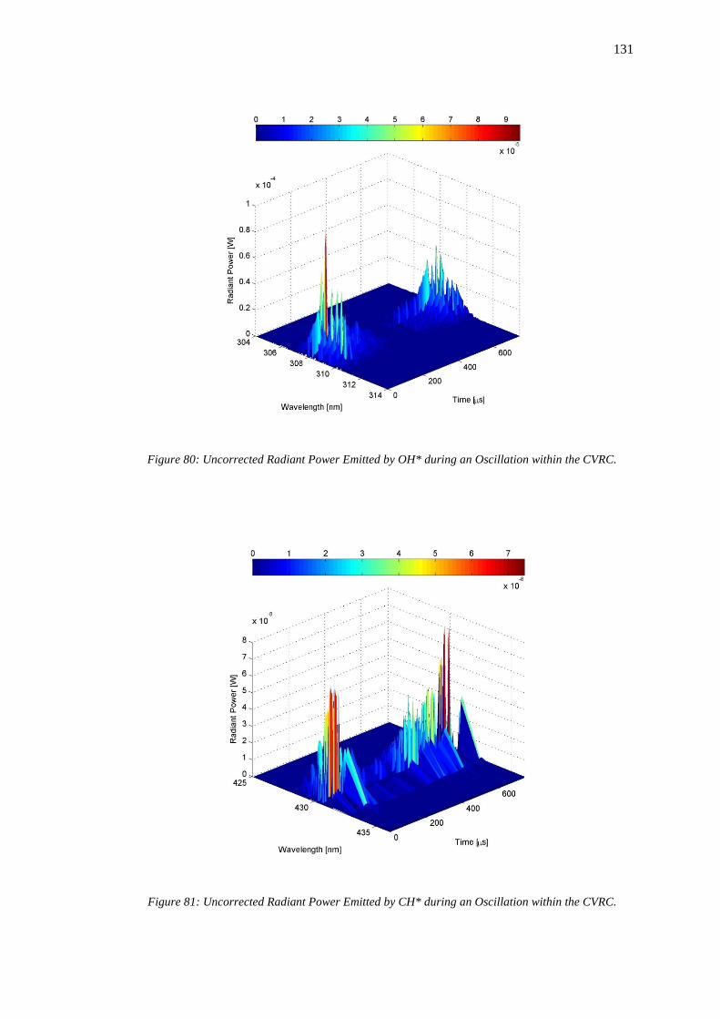
131
Figure 80: Uncorrected Radiant Power Emitted by OH* during an Oscillation within the CVRC.
Figure 81: Uncorrected Radiant Power Emitted by CH* during an Oscillation within the CVRC.

132
Figure 82: Uncorrected Combined Radiant Power Spectra Emitted by OH* and CH* during an Oscillation within the CVRC. The OH* Spectra are Located on the Left Hand Side of the Plot and the
CH* Spectra are Located on the Right.The CH* spectra are multiplied x500.
From Figure 80 and Figure 81 it is evident that during the oscillation the model predicts the
emission spectra uncorrected for absorption to vary with a phase similar to that of the oscillation
cycle. The OH* spectrum varies by more than an order of magnitude during the cycle. The
model predicts that the OH* emission peak occurs at 308.3 nm; though the peak at this
wavelength varies with the cycle it does remain the maximum for most of the oscillation.
Similar behaviour occurs with the CH* spectra; the spectra does vary during the oscillation
cycle, however the model predicts that the spectrum only varies within the range of an order of
magnitude. The model predicts that the CH* emission peak occurs at a wavelength of 430.5
nm. Comparing Figure 80 and Figure 81 it is clear that the radiant power emitted from OH* is
approximately three order of magnitude greater than that emitted from CH* in the CVRC based
on the computational data.
133
Figure 82 qualitatively shows that the CH* an OH* emissions vary with an approximately
similar phase during the oscillation, albeit the CH* signal is 3 orders of magnitude lower than
the OH* signal. Despite the large discrepancy of the relative spectral radiant power levels to
the experimental spectrum shown in Figure 64, the model produces a combined spectrum
shown in Figure 82 ,where the OH* emission strength is much larger than the CH* emission
strength for the CVRC, which agrees with qualitatively with the time average spectrum shown
in Figure 64.
5.2 Resultant Emission of OH* and CH* Corrected for Absorption
In this section the absorption corrected emission spectra for OH* and CH* are presented in a
similar fashion as before; the spectra are tracked through time. OH* and CH* resultant
emissions are plotted on separate spectral figures to get a scope on the magnitudes of the
different spectra. The different spectra are then combined into a single figure to provide a
qualitative comparison of the spectra yet again. The resultant absorption corrected spectra for
OH* is displayed in Figure 83 and the resultant absorption corrected spectra for CH* is
displayed in Figure 84. The combine spectra are displayed in Figure 85, where the CH* spectra
are multiplied by a factor 100 in order for the spectra to be qualitatively comparable.

134
Figure 83: Absorption Corrected Radiant Power Emitted by OH* during an Oscillation within the CVRC.
Figure 84: Absorption Corrected Radiant Power Emitted by CH* during an Oscillation within the CVRC.

135
Figure 85: Absorption Corrected Combined Radiant Power Spectra Emitted by OH* and CH* during an Oscillation within the CVRC. The OH* Spectra are Located on the Left Hand Side of the Plot and
the CH* Spectra are Located on the Right. The CH* spectra are multiplied x100.
As with the figures associated with the uncorrected spectra, the data from Figure 83 and Figure
84 show a variation in time. The comparison between Figure 80 and Figure 83 reveals that the
OH* signal is predicted by the model to decrease by almost an order of magnitude due to
absorption based signal attenuation along the optical path length within the probe volume.
When comparing Figure 81 and Figure 84 evidence of signal attenuation during the cycle
appears negligible as predicted by the model. This suggests that the combustion domain may
be optically thick with respect to the spectral range of OH*, while it is optically thin with respect
to the spectral range of CH*.
A qualitative comparison between Figure 82 and Figure 85 shows that the spectral emission
behaviour with respect to time does not differ between the absorption corrected and uncorrected
signals. It is interesting to note that for the absorption corrected spectra, especially that of OH*
136
show an increase in the spectral detail. This is because the main emission peak is significantly
absorbed, the less significant peaks are not as affected by the absorption and hence they stand
out more in the absorption corrected spectra of Figure 85 than the uncorrected spectra of Figure
82. A more detailed investigation of the absorption effects is done in a later section.
5.3 Time Averaged Spectra
To at least directly compare the numerical data with the experimental data on a qualitative level
the time averaged spectra over one oscillation produced by the computational model are
presented in this section. This data is not phase-average and thus only serves as a proof of
principle. The spectra of the uncorrected emissions of OH* and CH* are displayed in Figure
86 and Figure 87 respectively.
The combine uncorrected emission spectra of OH* and CH* is displayed in Figure 88, while
the absorption corrected combine emission spectrum is shown in Figure 89. The CH* spectra
of Figure 88 and Figure 89 are plotted on a separate axis which is scale accordingly. The radiant
power of the CH* spectrum is approximately three orders of magnitude lower than that of OH*
and is therefore predicted to be negligible when compare to OH*. The axes were scaled
differently in order for the spectra to be compare directly without any loss of precision or
information.

137
Figure 86: Uncorrected Time Averaged Spectrum of OH* during One Oscillation.
Figure 87: Uncorrected Time Averaged Spectrum of CH* during One Oscillation.

138
Figure 88: Uncorrected Time Averaged Combined Spectrum of OH* and CH* during One Oscillation.
Figure 89: Absorption Corrected Time Averaged Combined Spectrum of OH* and CH* during One Oscillation

139
A comparison between Figure 88 and Figure 89 shows that while the CH* spectrum is predicted
to be unaffected by absorption effects, the OH* spectrum is predicted to be significantly
reduced due to absorption. The shape of the OH spectrum also changes with respect to the
uncorrected and absorption corrections. This evidence further suggests that the CVRC
combustion medium is optically thick for emissions produced by OH*.
5.4 Temporal Measure of Signal Transmission
A temporal evolution of the transmissivity of the CVRC combustion medium for the OH* and
CH* spectra is investigate in this section. The study will reveal if and when the combustion
medium becomes optically thick or thin for the spectra of OH* and CH* during a
thermoacoustic cycle.
It is sometimes hard to gauge the effect of absorption from these plots; it was decided to that
an isometric view was used to give an overall view of the data spread, while views from the
temporal and spectral axes are meant to show the variation of the transmissivity with respect to
those properties.
The transmissivity of the CVRC combustion medium with respect to the spectrum and time for
OH* is shown below in Figure 90, Figure 91 and Figure 92.

140
Figure 90: Temporal Evolution of the Spectral Transmissivity of the CVRC Combustion Medium within the Probe Volume for OH* during the Period of One Cycle. (Isometric View)
Figure 91: Temporal Evolution of the Spectral Transmissivity of the CVRC Combustion Medium within the Probe Volume for OH* during the Period of One Cycle. (Temporal View)

141
Figure 92: Temporal Evolution of the Spectral Transmissivity of the CVRC Combustion Medium within the Probe Volume for OH* during the Period of One Cycle. (Spectral View)
Figure 90 provides evidence that the OH* spectrum is significantly affected by absorption
during a cycle of the CVRC. The most absorption occurs in the approximate spectral range of
307-310nm as seen in Figure 92; this range is over the main emission peak of OH* at 308.3nm.
Additionally, it should be note that the absorption occurs over the range where the bulk of
spectral radiant power comes from. This data further reinforces the idea that the CVRC
combustion medium is optically thick for OH*.
Although significant absorption occurs over the OH* spectrum for most of the cycle, Figure 91
shows a period of time (300-400𝜇𝜇𝑠𝑠) in the cycle where the CVRC combustion medium becomes
optically thin OH* emissions. Curiously, when this data in this time frame is compared to the
data from Figure 80 the lack absorption correlates to the lack of raw spontaneous emission.
The transmissivity of the CVRC combustion medium with respect to the spectrum and time for
OH* is shown below in Figure 90, Figure 91 and Figure 92.
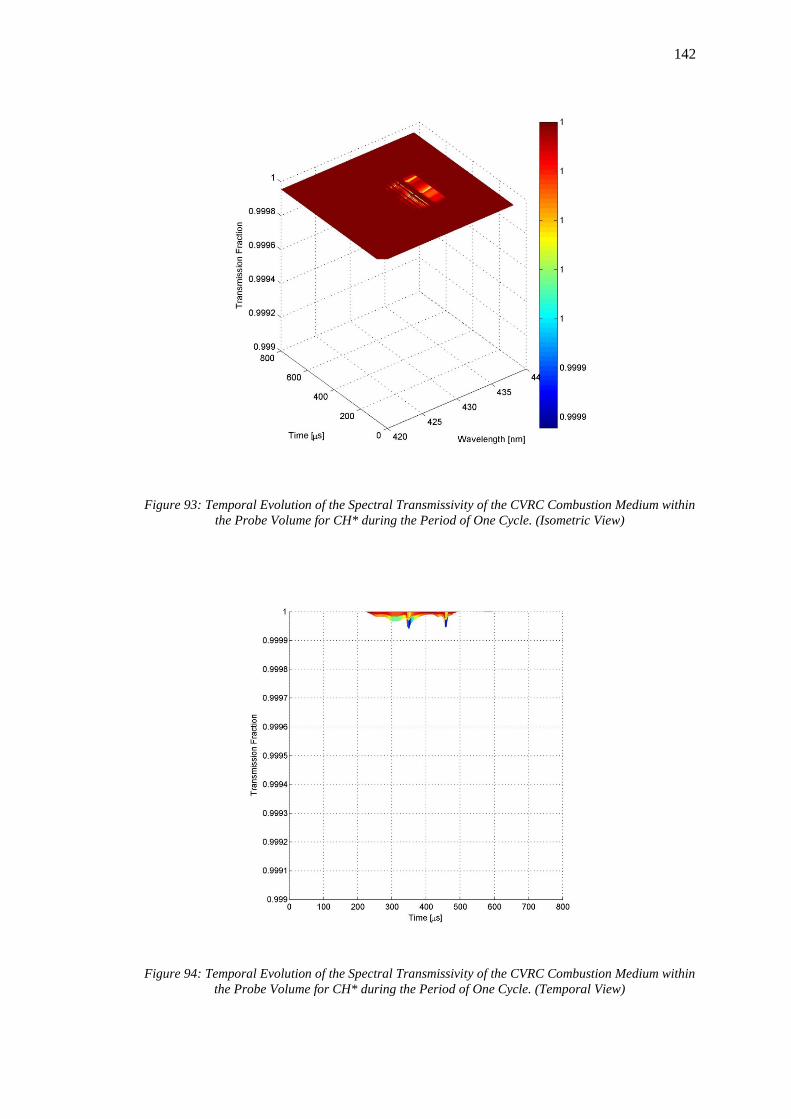
142
Figure 93: Temporal Evolution of the Spectral Transmissivity of the CVRC Combustion Medium within the Probe Volume for CH* during the Period of One Cycle. (Isometric View)
Figure 94: Temporal Evolution of the Spectral Transmissivity of the CVRC Combustion Medium within the Probe Volume for CH* during the Period of One Cycle. (Temporal View)

143
Figure 95: Temporal Evolution of the Spectral Transmissivity of the CVRC Combustion Medium within the Probe Volume for CH* during the Period of One Cycle. (Spectral View)
Figure 93 supports the evidence that the CH* spectrum is predicted to not be significantly
affected by absorption during a cycle of the CVRC. Figure 94 and Figure 95 clearly shows that
absorption effects predicted by the only manage to attenuate the full spectral CH* signal during
a cycle by less than 1/10000th.
5.5 Spatial Measure of Signal Transmission
From the preceding data it appears that the combustion domain may be optically thick for
emissions produced by OH* and optically thin for the emissions produced by CH*. It is still
yet unclear as to how optically thick or thin the CVRC combustion medium is predicted to be
for OH* and CH*. Therefore a study into the optical density of the medium over the optical
path of the probe volume is conducted in order to determine the severity of the optical
absorption effects on the optical emissions. Data regarding the spatial distribution of the

144
absorption fraction per the spectral range of OH* and CH* are plotted at key time intervals
corresponding to the expected approximate maxima and minima of absorption.
The spectral absorption fraction per optical distance from the optic port is plotted for OH* at
the time intervals 75, 375 and 625 𝜇𝜇𝑠𝑠 below in Figure 96, Figure 97 and Figure 98 respectively.
Figure 96: Spatial Distribution of the Spectral Absorption Fraction of OH*in the Probe Volume at the Time Interval 75𝜇𝜇𝑠𝑠.
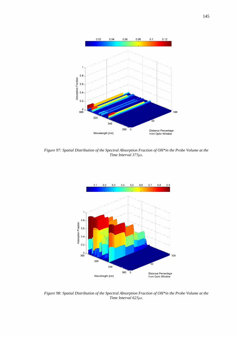
145
Figure 97: Spatial Distribution of the Spectral Absorption Fraction of OH*in the Probe Volume at the Time Interval 375μs.
Figure 98: Spatial Distribution of the Spectral Absorption Fraction of OH*in the Probe Volume at the Time Interval 625μs.

146
From Figure 96 and Figure 98 it is clear that the spectral signal produced at the far end of the
combustion chamber by OH* at t = 75 and 625𝜇𝜇𝑠𝑠, which correspond to approximate maxima
of spectral absorption in time, is completely attenuated at the main emission peaks produced by
the time the emission signal reaches the optic port. Because the domain is axisymmetric, this
data predicts that most, if not all, of the spectral signal produced by OH* measured by the
spectrometer is emitted by OH* at a location right near the optic port window.
Strangely enough, the spatial distribution of the spectral absorption fraction of Figure 97,
corresponding to an approximate minimum of spectral absorption in time, shows that the OH*
emission signal is barely attenuated. Counter-intuitively, it appears that the CVRC
combustion domain becomes optically thin when the raw emission signal is at its lowest.
The behaviour of the attenuation of the OH* emission signal correlates with the spatial
distribution (axisymmetric) of the gas state data from the computational model. This strongly
suggests that the number density of OH* and OH are linked, and possibly proportional, and
when their productions wanes so too does the attenuation of the emission signal due to
absorption.
The spectral absorption fraction per optical distance from the optic port is plotted for CH* at
the time intervals 75, 375 and 625 𝜇𝜇𝑠𝑠 below in Figure 99, Figure 100 and Figure 101
respectively.
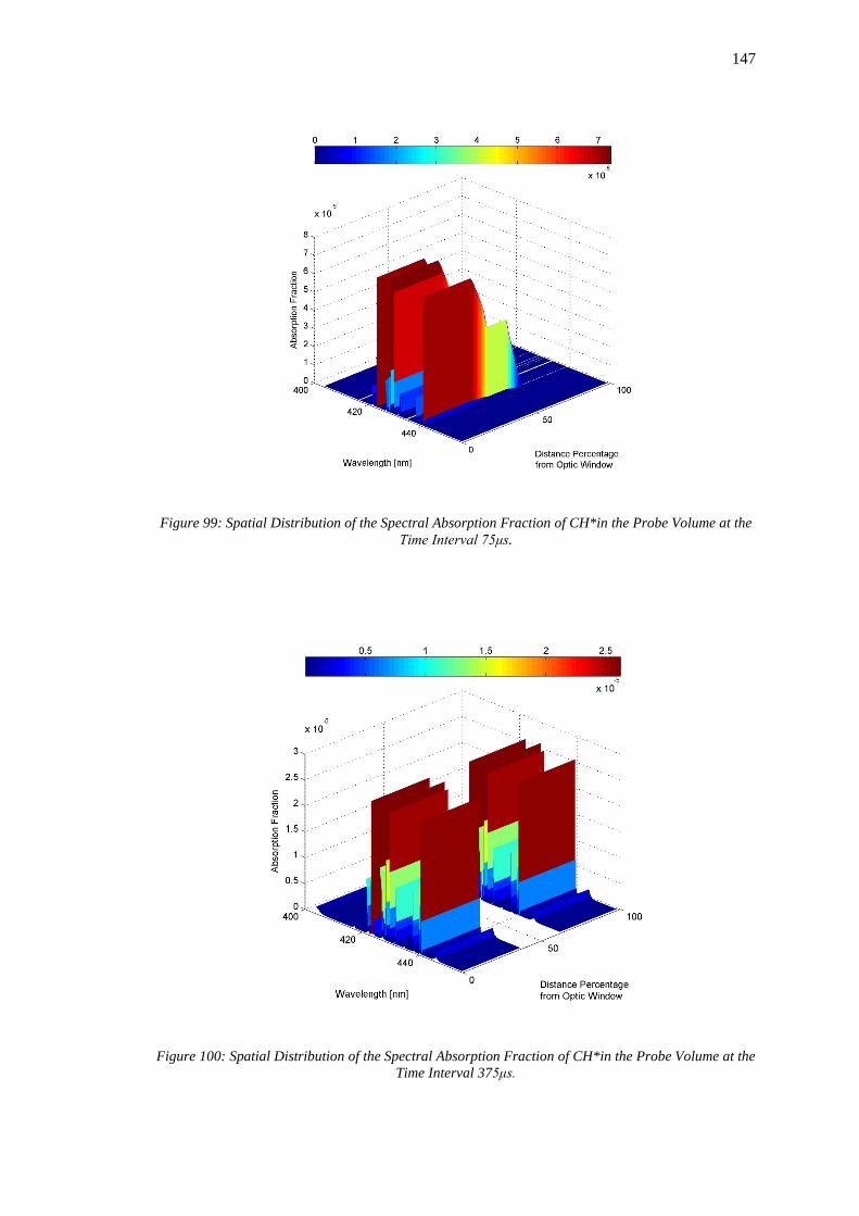
147
Figure 99: Spatial Distribution of the Spectral Absorption Fraction of CH*in the Probe Volume at the Time Interval 75μs.
Figure 100: Spatial Distribution of the Spectral Absorption Fraction of CH*in the Probe Volume at the Time Interval 375μs.

148
Figure 101: Spatial Distribution of the Spectral Absorption Fraction of CH*in the Probe Volume at the Time Interval 625μs.
Although there seems to be a variation in the absorption fraction along the optical path length,
the maximum amount absorption found in Figure 99, Figure 100 and Figure 101 are
negligible.
A note about the spatial evolution of the absorption fraction: in each case the optical
absorption fraction appears to make a “step” in its value as position is varied along the optical
path length. This “step” is the result of a local band or spot of higher number density of
absorbers. This could be the direct result of the axisymmetric assumption, where when the
probe volume is formed by “unwrapping” the 2D axisymmetric computational domain into
3D a higher absorber number density band then becomes a ring or short cylinder in 3D space.
When this torus is collapsed into the 1D approximation for the probe volume the higher
number density influences the number density of the shell making the shell a 1D local spot of

149
higher absorber number density. Effectively, the “steps” in the absorption fraction along the
optical path length are an artefact of the model’s domain assumption.
5.6 Number Density Correlation
Because the model predicts a causal link between the number density of the emitters and
absorbers with the strength of the emissions collected by the spectrometer, an attempt to
correlate the domain number density with the CVRC combustion medium to transmit the
emissions produced by OH* and CH* is performed. Additionally, since 𝐶𝐶𝐶𝐶2 emits within the
spectral range of interest as shown in the experimental measurement data in Figure 64, a
quantification of the level of absorption that the spectra from OH* and CH* emissions will
experience must be made.
The temporal evolution of the change in volume averaged number density within the probe
volume, with special interest in species that may influence the spectrum, and the overall
transmissivity of the CVRC combustion medium with respect to OH* is shown in Figure 102,
and similarly for CH* in Figure 103.
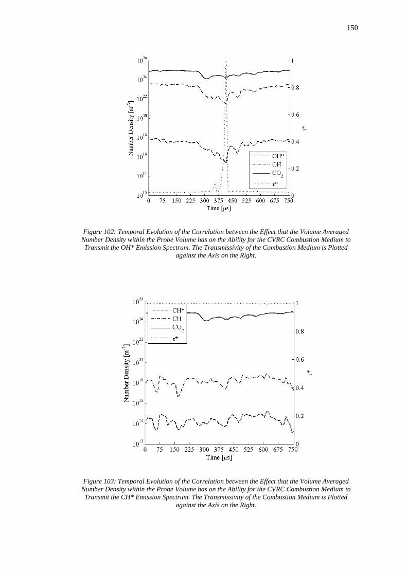
150
Figure 102: Temporal Evolution of the Correlation between the Effect that the Volume Averaged Number Density within the Probe Volume has on the Ability for the CVRC Combustion Medium to Transmit the OH* Emission Spectrum. The Transmissivity of the Combustion Medium is Plotted
against the Axis on the Right.
Figure 103: Temporal Evolution of the Correlation between the Effect that the Volume Averaged Number Density within the Probe Volume has on the Ability for the CVRC Combustion Medium to Transmit the CH* Emission Spectrum. The Transmissivity of the Combustion Medium is Plotted
against the Axis on the Right.
151
In agreement with the data before it Figure 102 shows that the optic model predicts the
transmissivity of the CVRC combustion medium is optically dense for OH* emissions during
a cycle, except for a small time interval where it becomes optically thin. The trend of the
production of the number density data backs up this conclusion quite well. This conclusion can
be further verified from the verification data of Figure 90.
Similarly, the data plotted in Figure 103 clearly shows that CVRC combustion medium is
completely transparent to the emissions from CH* and all the data preceding this agree
completely.
From Figure 102 and Figure 103 the volume averaged 𝐶𝐶𝐶𝐶2 number density is much higher than
that of OH or CH. The time averaged volume averaged 𝐶𝐶𝐶𝐶2 number density is approximately
1025𝑔𝑔−3, while the time averaged volume averaged number densities of OH and CH are
approximately 1023𝑔𝑔−3 and 1018𝑔𝑔−3 respectively. Since OH is the natural optical absorber
of OH* emissions and it has been determined that the CVRC combustion medium is optically
thick with respect to OH* emissions then it is worrisome that the 𝐶𝐶𝐶𝐶2 number density is two
orders of magnitude greater than that of OH.
Because 𝐶𝐶𝐶𝐶2 is a triatomic molecule its spectrum is complex and its corresponding spectral
data has yet to be determined for each of the transitions. Measurements however, have been
made to determine it absorption cross section over a wide spectral range for different
temperatures [55]. The macroscopic cross section of 𝐶𝐶𝐶𝐶2 can be described using the following
empirical relation:
ln�𝜎𝜎(𝜆𝜆,𝑇𝑇)� = 𝑎𝑎(𝑇𝑇) + 𝑏𝑏(𝑇𝑇)𝜆𝜆 (146)
𝑎𝑎 = 𝑔𝑔1 + 𝑔𝑔2𝑇𝑇 +𝑔𝑔3𝑇𝑇
𝑏𝑏 = 𝑑𝑑1 + 𝑑𝑑2𝑇𝑇 +
𝑑𝑑3𝑇𝑇

152
, where 𝑇𝑇 is in the units 1000K, the wavelength 𝜆𝜆 is in units of 100nm, the absorption cross
section is in units 10−19𝑔𝑔𝑔𝑔2 and the constants are given by:
𝑔𝑔1 = 0.05449 𝑑𝑑1 = 1.991
𝑔𝑔2 = 0.13766 𝑑𝑑2 = −0.17125
𝑔𝑔3 = 23.529 𝑑𝑑3 = −14.694
Using the wavelengths 280nm and 460nm to set the bounds of the spectral range of emission,
based off the experimental data from Figure 64, the corresponding absorption cross sections are
calculated using Equation 122 as 𝜎𝜎280𝑛𝑛𝑚𝑚 = 7.95 × 10⁻²¹𝑔𝑔𝑔𝑔2 and 𝜎𝜎460𝑛𝑛𝑚𝑚 = 2.23 ×
10−24𝑔𝑔𝑔𝑔2. For an optical path length equivalent to that of the width of the CVRC chamber,
𝑧𝑧 = 0.045𝑔𝑔. Now the transmission fraction can be calculated using a different form Equation
87, which includes the cross section of interaction 𝜎𝜎, with a number density of 𝐶𝐶𝐶𝐶2 assigned to
be 𝑁𝑁𝐶𝐶𝑂𝑂2 = 1025𝑔𝑔−3:
𝜏𝜏 = exp�−𝜎𝜎𝑁𝑁𝐶𝐶𝑂𝑂2𝑧𝑧�
The calculated transmission fraction in each case is then given by:
𝜏𝜏280𝑛𝑛𝑚𝑚 = exp(−(7.95 × 10⁻²⁵)(1025)(0.045)) = 0.699
𝜏𝜏460𝑛𝑛𝑚𝑚 = exp(−(2.23 × 10⁻²⁸)(1025)(0.045)) = 1.00
At each of the emission peaks the absorption cross sections and the transmission fractions are
calculated to be:
𝜎𝜎300𝑛𝑛𝑚𝑚 = 3.21 × 10⁻²¹𝑔𝑔𝑔𝑔2 𝜏𝜏300𝑛𝑛𝑚𝑚 = 0.865
𝜎𝜎430𝑛𝑛𝑚𝑚 = 8.73 × 10⁻²⁴𝑔𝑔𝑔𝑔2 𝜏𝜏430𝑛𝑛𝑚𝑚 = 1.00
Therefore the effect of absorption due to 𝐶𝐶𝐶𝐶2 is not insignificant with respect to OH*, but is
insignificant with respect to CH*. As such, the hypothesis that the CVRC combustion medium
is optically thick for OH* and optically thin for CH* remains the unchanged. The variation of

153
the cross sections and transmissivity for an optical path length of 0.045m and a number density
of 𝐶𝐶𝐶𝐶2 of 1025𝑔𝑔−3 with temperature are shown in Figure 104 and Figure 105. The variation
in transmissivity with 𝐶𝐶𝐶𝐶2 number density at a temperature of 2500K is shown in Figure 106.
Figure 104: Cross Section of 𝐶𝐶𝐶𝐶2 over the Spectrum of Interest for Different Temperatures.
Figure 105: Transmissivity of 𝐶𝐶𝐶𝐶2 over the Spectrum of Interest for Different Temperatures.

154
Figure 106: Transmissivity of 𝐶𝐶𝐶𝐶2 over the Spectrum of Interest for Different Number Densities.
155
6. CONCLUSION AND SUMMARY
6.1 Experimental and Numerical Spectra Comparison
The spectral frequencies of the emissions from OH* and CH* compare well between the optical
model and the experimental data. The relative emission strengths between OH* and CH*
predicted by the optical model, however, do not correspond well with the relative emission
strengths measured in experiment, even with the geometric and absorption corrections to the
raw emissions based on the CFD data.
The OH* integrated signal predicted by the optical model is approximately 2.5 to 3 orders of
magnitude greater than the predicted integrate CH* signal, whereas the experimental data
shows a relative signal difference between OH* and CH* to be approximately 1 order of
magnitude. Assuming that the equivalence ratio of the CFD simulation for the CVRC has a
very close agreement to the CVRC experiment equivalence ratio, then the discrepancy might
lie in the detailed kinetics model predicting the production levels of the OH and CH radicals
and their excited counterparts.
The overall error of the optical model is based on the error of the CFD simulation, and therefore
as the error of the CFD simulation decreases, the comparison between the experiment and the
CFD simulation becomes better.
The oxidizer rich propellant combination of decomposed hydrogen peroxide and gaseous
methane in the CVRC means that a large mass of water is dumped into the system during
156
combustion. Water is inherently composed of a hydroxyl radical and monatomic hydrogen,
and therefore large amounts of hydroxyl radicals are dumped into the system. This could be the
main source for the high number density of the hydroxyl radical responsible for absorption of
the OH* emissions.
6.2 OH* Emissions and Optical Density
From the CFD data the optical model predicts that for the conditions of the CVRC the
combustion medium is optically opaque or optically thick within the measured probe volume
for the emissions produced by OH*. The production of OH* and OH within the probe volume
appears to be synchronous. The expected main production reaction of OH* in the flame reaction
zone involves the CH radical because the threshold activation energy is zero.
From the CFD model and the phase of the production of OH relative to OH* it appears that
besides the normal production of OH from other elementary reactions a decent level of
production of OH may come from the quenching of OH* due to collisions. The large number
of collisions is due to the high pressure, especially during the upper limit of the fluctuation
during a thermoacoustic cycle. The enhanced quenching of OH* may help to drain the
concentration of CH radicals in the locale of the production reaction of OH*.
Because the elementary reactions involving the production of OH* do not involve the OH
radical as a reactant, it would be logical to assume that if a large portion of the OH in the system
was produced by other elementary reactions, assuming that quenching was negligible, then the
production phase of OH* and OH during a thermoacoustic cycle may not be synchronous within
an acceptable confidence level (at least qualitatively comparable).
Because 𝐶𝐶𝐶𝐶2 may absorb within the spectral range emitted by OH* the notion of optical opacity
for the emissions of OH* is further reinforced. High number densities of 𝐶𝐶𝐶𝐶2 can greatly add
to the amount of absorption the OH* signal may encounter.

157
This ultimately suggests that the signal emissions and absorption is greatly affected by the
pressure of the system, but not in a way most expected. The pressure affects the resultant
emission signals indirectly through the production of OH.
One important note about the OH* emissions measured: due to the optical opacity, the signal
collected may only be at the very near to the combustor wall. At this region the main
combustion reactions are unlikely to occur; the OH* emissions may actually be the result of the
recombination of monatomic oxygen and hydrogen in a slightly cooler part of the combustion
medium. This reaction is sometimes referred to as the “thermal production” of OH*.
6.3 CH* Emissions and Optical Density
From the CFD data the optical model predicts that for the conditions of the CVRC the
combustion medium is optically transparent or optically thin within the measured probe volume
for the emissions produced by CH*. As with the case of OH and OH*, the production of CH*
and CH within the probe volume appears to be synchronous.
Because the CVRC is oxidizer rich the production of 𝐶𝐶2 is almost negligible when compared
with other radicals; hence, the main production reaction of CH* involves 𝐶𝐶2𝐻𝐻 and monatomic
oxygen. Furthermore, because the CVRC is oxidizer rich the general production of carbon
based radicals is expected to be lower than that of oxygen based radicals; the production of CH
in general is expected to be quite in comparison to OH.
In a similar fashion to OH, CH production seems to be the result of the quenching due to the
synchronicity of the production of CH* and CH during a thermoacoustic cycle. It is difficult to
say whether the quenching of CH* is stronger than that of OH* for the same collision partners
under the same conditions, but it does seem that the collisional quenching of OH* may be
stronger than that of CH* based on the reaction rate equations. This effect may be part of the
cause as to why the number density of CH is much lower than OH (a few orders of magnitude
lower) allowing for the absorption of the CH* emissions to be negligible.

158
As a consequence the emission signals of CH* during the entire thermoacoustic cycle during
combustion within the CVRC is fully line-of-sight integrated with respect to the chamber width
because of the optical transparency at the range of frequencies emitted by CH*. Thus, the signal
collected by CH* may be considered somewhat spatially resolved with respect to the axial
location of the chamber; the signal can also therefore be considered to include the information
of the emissions produced by CH* of the main reaction zone.
6.4 OH* and CH* as Markers for Heat Release in the CVRC
Based on the predictions of the optical model OH* is not a good marker for heat release. The
OH* signal collected does not correspond with the main flame reaction zone. Part of the CH*
signal collected corresponds to the main reaction zone, however it is not clear how much the
production of CH* is affected by aerodynamic strain rate, especially in the presence of high
amplitude pressure oscillations. Additionally, because of the acoustic oscillations the mixing of
the propellants is enhanced thus accelerating the increase in the local temperature due to heat
release; this leads to a flame acceleration due to the turbulence of the flow increasing the flame
area. The flame acceleration is also partly responsible for the increase in aerodynamic strain
rate. 𝐶𝐶𝐻𝐻∗ also suffers from a low signal to noise ratio, there is a large influence due to the
presence of the 𝐶𝐶𝐶𝐶2∗ emissions. It is unclear whether the 𝐶𝐶𝐻𝐻∗ emissions can be differentiated
from the 𝐶𝐶𝐶𝐶2∗ emissions from within the combustor during measurement.
Together the ratio of OH* to CH* might be able to give a spatially resolved measure of the
local equivalence ratio, however because chemiluminescence is a line of sight integrated
technique this makes it difficult to get a good approximation of the signal ratio between OH*
and CH*. In the case of the CVRC with it current propellant combination the ratio of the OH*
and CH* emission signals will not produce any useful information.
If the CH* signal is temporally resolved it might be useful as a quantitative heat release marker
in that it could be used to show the cycle and phase of the heat release with respect to pressure
oscillations. It should be noted that the broadband absorption due to 𝐶𝐶𝐶𝐶2 affects the emissions

159
of OH* significantly, but affects the emissions of CH* insignificantly during a thermoacoustic
cycle. These effects ultimately do not change the outcome of the predictions of the optic model
with respect to the CVRC data.
6.5 OH* and CH* as Markers for Heat Release in the General Case
If the ground state number densities of OH and CH for a specific propellant combination are
predicted to be low enough then both emission signals for OH* and CH* could be used as
measures of heat release in a partial spatially resolved sense. The line-of-sight integrated
measurements may be used to estimate the dynamics associate with heat release within a small
region, where the tighter the focus of the measured probe volume the more spatially resolved
the estimate can be.
It should be emphasized that the chemiluminescence measurements are only useful if the
absorbing species’ number densities (OH, CH and 𝐶𝐶𝐶𝐶2) are below a certain threshold to allow
for full line-of-sight integrated measurements along the width of the chamber.
Lastly, prudent care needs to be taken when considering chemiluminescence measurements for
a new set of conditions or a new combustion experiment. For each case the chemistry is unique
and therefore the production of all the possible radicals and chemical species temporally and
spatially is unique to each case. If the location of measurement has the possibility of self-
absorption influencing the measurements then the technique of using chemiluminescence as an
optical diagnostic tool is not recommended.
6.6 Future Work
• Retrofit gaseous oxygen as a replacement for decomposed hydrogen peroxide as the
oxidizer in an attempt to reduce the levels of the hydroxyl radical in the system.
• Absorption spectroscopy specific to the CVRC conditions.
o OH: Determine the exact levels of absorption due to OH and infer what the
number density may be at a specific location. This can be compared to the CFD

160
data for a better measure of the CFD simulation to predict conditions inside the
chamber.
o 𝐶𝐶𝐶𝐶2: The absorption cross section data has been extrapolated for the spectral
range useful for the measurements based in the CVRC. A measurement of the
spectral range between the emissions produced by OH* and CH* might serve
as a good approximation for the data.
• Cross-beam correlation using a “grid” of probe volumes created from multiple
measurement points at the same axial location. The measurement locations will form
probe volumes that cross the chords of the cross section of the chamber where they will
be orthogonal to any of the other probe volumes within the chamber. By correlating the
data measured by each probe volume it might be possible to construct a spatial profile
of the local specie number densities and emissions due to chemiluminescent reactions
across the chamber cross section at a specific axial location/s.

REFERENCES

161
REFERENCES
[1] R. E. Sonntag, C. Borgnakke and G. J. van Wylen, Fundamentals of Thermodynamics,
6th Ed., Hoboken: John Wiley & Sons, Inc., 2003.
[2] B. N. Taylor and P. J. Mohr, Fundamental Physical Constants, NIST Chemistry
Webbook, 2010.
[3] N. M. Laurendau, Statistical Thermodynamics: Fundamentals and Applications, New
York: Cambridge University Press, 2005.
[4] O. P. Sutton and O. Biblarz, Rocket Propulsion Elements, 8th Ed., Hoboken: John Wiley
& Sons, Inc., 2010.
[5] S. R. Turns, An Introduction to Combustion, Concepts and Applications, 3rd Ed., New
York: McGraw-Hill, 2012.
[6] R. Bowen, “Free Radicals and Reactive Oxygen,” Colorado State University, 16 August
2003. [Online]. Available:
http://www.vivo.colostate.edu/hbooks/pathphys/misc_topics/ros.gif. [Accessed 22 July
2015].
162
[7] U. o. C. Davis, “The Arrhenius Law: Activation Energies,” [Online]. Available:
http://chemwiki.ucdavis.edu/Physical_Chemistry/Kinetics/Modeling_Reaction_Kineti
cs/Temperature_Dependence_of_Reaction_Rates/The_Arrhenius_Law/The_Arrhenius
_Law%3A_Activation_Energies. [Accessed 22 July 2015].
[8] Wikipedia, “Molecular vibration,” Wikipedia, the free encyclopedia, 17 February 2015.
[Online]. Available:
http://en.wikipedia.org/w/index.php?title=Molecular_vibration&oldid=647594704.
[Accessed 1 June 2015].
[9] G. Smith, D. Golden, M. Frenklach, N. Moriarty, B. Eiteneer, M. Goldenberg, C.
Bowman, R. Hanson, S. Song, W. J. Gardiner, V. Lissianski and Z. Qin, “GRI Mech
3.0,” [Online]. Available: http://www.me.berkeley.edu/gri_mech/. [Accessed 1 June
2015].
[10] A. Gaydon, The Spectroscopy of Flames, London: Chapman and Hall Ltd., 1957.
[11] A. Gaydon and H. Wolfhard, “Flames,” Chapman and Hall Ltd., London, 1960.
[12] J. Hall and E. Petersen, “An Optimized Kinetics Model for OH Chemiluminescence at
High Temperatures and Atmospheric Pressures,” Journal of Chemical Kinetics, vol. 38,
pp. 714-724, 2006.
[13] V. Nori and J. Seitzman, “CH* chemiluminescence modeling for combustion
diagnostics,” Proceedings of the Combustion Institute, vol. 32, pp. 895-903, 2009.
[14] M. Tamura, P. Berg, J. Harrington, J. Luque, J. Jeffries, G. Smith and D. Crosley,
“Collisional Quenching of CH(A), OH(A) and NO(A) in Low Pressure Hydrocarbon
Flames,” Combustion and Flame, vol. 114, no. 3-4, pp. 502-514, 1998.

163
[15] C. Haber, “An investigation into the origin, measurement and application of
chemiluminescent species from premixed flames.,” Virginia Polytechnic Institute,
Blacksburg, 2000.
[16] G. Smith, J. Luque, C. Park and J. C. D. Jeffries, “Low pressure flame determinations
of rate constants for OH(A) and CH(A) chemiluminescence,” Combustion and Flame,
vol. 131, no. 1-2, pp. 59-69, 2002.
[17] K. Devriendt, H. Van Look, B. Ceursters and J. Peeters, “Kinetics of formation of
chemiluminescent CH by the elementary reactions of C2H with O and O2: a pulse laser
photolysis study,” Chemical Physical Letters, vol. 261, pp. 450-456, 1996.
[18] G. Smith, C. Park and J. Luque, “A note on chemiluminescence in low-pressure
hydrogen and methane-nitrous oxide flames,” Combustion and Flame, vol. 140, no. 4,
pp. 385-389, 2005.
[19] T. Kathrotia, U. Riedel, A. Seipel and K. Moshammer, “Experimental and numerical
study of chemiluminescent species in low-pressure flames,” Applied Physics B: Lasers
and Optics, vol. 107, pp. 571-584, 2012.
[20] G. Smith, C. Park, J. Schneiderman and J. Luque, “C2 Swan band laser-induced
fluorescence and chemiluminescence in low-pressure hyrdrocarbon flames,”
Combustion and Flame, vol. 141, no. 1-2, pp. 66-77, 2004.
[21] M. Slack and A. Grillo, “High Temperature Rate Coefficient Measurements of CO+O
Chemiluminescence,” Combustion and Flame, vol. 59, pp. 189-196, 1985.
[22] V. Nori and J. Seitzman, “Evaluation of Chemiluminescence as a Combustion
Diagnostic under Varying Operating Conditions,” in AIAA, Reno, 2008.

164
[23] J. Lee and D. Sanatavicca, “Experimental Diagnostics for the Study of Combustion
Instabilities in Lean Premixed Flames,” Journal of Propulsion and Power, vol. 19, no.
5, pp. 735-750, 2003.
[24] G. Herzberg, Spectra of Diatomic Molecules, New York: D. Van Nostrand Company,
Inc., 1957.
[25] H. Najm, K. O.M., P. Paul and P. Wyckoff, “A Study of Flame Observables in Premixed
Methane-Air Flames,” Combustion Science an Technology, vol. 140, pp. 369-403, 1998.
[26] H. Najm, O. Knio and P. Paul, “Role of Transport Properties in the Transient Response
of Premixed Methane/Air Flames,” Proceedings of the Combustion Institute, vol. 29,
pp. 1713-1720, 2002.
[27] T. Muruganandam, B.-H. Kim, M. Morrell, V. Nori, M. Patel, B. Romig and J.
Seitzman, “Optical equivalence ratio sensors for gas turbine combustors.,” Proceedings
of the Combustion Institute, vol. 30, pp. 1601-1609, 2005.
[28] T. Garcia-Armingol, Y. Hardalupas, A. Taylor and J. Ballester, “Effect of local flame
properties on chemiluminescence based stoichiometry measurement,” Experimental
Thermal and Fluid Science, vol. 53, pp. 93-103, 2014.
[29] B. Ayoola, R. Balachandran, J. Frank, E. Mastorakos and C. Kaminski, “Spatially
resolved heat release rate measurements in turbulent premixed flames,” Combustion and
Flame, vol. 144, pp. 1-16, 2006.
[30] C. Panoutsos, Y. Hardalupas and A. Taylor, “Numerical evaluation of equivalence ratio
measurement using OH* and CH* chemiluminescence in premixed and non-premixed
methan-air flames,” Combustion and Flame, vol. 156, no. 2, pp. 273-291, 2009.

165
[31] N. e. Centre, “Nature of Radiation,” [Online]. Available: https://www.nde-
ed.org/EducationResources/CommunityCollege/RadiationSafety/theory/nature.htm.
[Accessed 22 July 2015].
[32] F. Pedrotti, L. Pedrotti and L. Pedrotti, Introduction to Optics, 3rd Ed., New Delhi:
Pearson Prentice Hall, 2007.
[33] I. E. 360, “Solid Angle and Brightness Theorem,” [Online]. Available:
http://www.globalspec.com/reference/21462/160210/appendix-a-solid-angle-and-the-
brightness-theorem. [Accessed 22 July 2015].
[34] Y. Cengel, Heat and Mass Transfer: A Practical Approach, 3rd Ed., New York:
McGraw-Hill, 2006.
[35] A. Eckbreth, Laser Diagnostics for Combustion Temerature and Species, 2nd Ed.,
Amsterdam: Gordon and Breach Publishers, 1995.
[36] A. Siegman, Lasers, Mill Valley: University Science Books, 1986.
[37] R. Lucht, Notes: ME 687 Laser Diagnostics of Reacting Flow, West Lafayette: Purdue
University, 2014.
[38] R. Eisberg and R. Resnick, Quantum Physics of Atoms, Molecules, Solids, Nuclei and
Particles, 2nd Ed., New York: John Wiley and Sons, 1985.
[39] S. Macheret, Notes on Plasmas and Electric Discharges, West Lafayette: Purdue
University, 2015.
[40] A. A. Fridman and L. Kennedy, Plama Physics and Engineering, New York: Taylor
and Francis Routledge, 2004.

166
[41] R. Learner, “The Influence of Vibration-Rotation Interaction on Intensities in the
Electronic Spectra of Diatomic Molecules. I. The Hydroxyl Radical.,” Proceedings of
the Royal Society of London, Series A, Mathematical and Physcial Sciences., vol. 269,
no. 1338, pp. 311-326, 1962.
[42] D. Crosley and R. Lengel, “Relative Transition Probabilities and the Electronic
Transition Moment in the A-X System of OH.,” Journal of Quantitative Spectroscopy
and Radiative Transfer, vol. 15, pp. 579-591, 1975.
[43] I. Chidsey and D. Crosley, “Calculate Rotational Transition Probabilities for the A-X
System of OH.,” Journal of Quantitative Spectroscopy and Radiative Transfer, vol. 23,
pp. 187-199, 1980.
[44] J. Luque and D. Crosley, “Transition probabilties in the A-X electronic system of OH.,”
Journal of Chemical Physics, vol. 109, no. 2, pp. 439-448, 1998.
[45] J. Luque and D. Crosley, “Electronic transition moment and rotational transition
probabilities in CH. I. A-X system.,” The Journal of Chemical Physics, vol. 104, no. 6,
pp. 2146-2155, 1996.
[46] A. Schadee, “Unique Definitions for the Band Strength and the Electronic-Vibrational
Dipole Moment of Diatomic Molecular Radiative Transitions.,” Journal of Quantitative
Spectroscopy and Radiative Transfer, vol. 19, pp. 451-453, 1978.
[47] L. Williams and D. Crosley, “Collisional vibrational energy transfer of OH,” Journal of
Chemical Physics, vol. 104, no. 17, pp. 6507-6514, 1996.
[48] R. Copeland, M. Dyer and D. Crosley, “Rotational level development quenching of OH
and AD,” The Journal of Chemical Physics, vol. 82, no. 9, pp. 4022-4032, 1985.
167
[49] A. Brockhinke, J. Kruger, M. Heusing and M. Letzgus, “Measurement an simulation of
rotationally-resolved chemiluminescence spectra in flames.,” Applied Physics B, vol.
107, no. 3, pp. 539-549, 2012.
[50] Wikipedia, “Optical Fiber,” [Online]. Available:
https://en.wikipedia.org/wiki/Optical_fiber. [Accessed 22 July 2015].
[51] J. Humlicek, “An efficient method for evaluation of the complex probability function:
The Voigt function and its derivatives,” Journal of Quantitative Spectroscopy and
Radiative Transfer, vol. 21, no. 4, pp. 309-313, 1979.
[52] K. L. Letchworth and D. Benner, “Rapid and accurate calculation of the Voigt function,”
Journal of Quantitative Spectroscopy and Radiative Transfer, vol. 107, pp. 173-192,
2007.
[53] J. Luque and D. Crosley, LIFBASE, Database and spectral simulation for diatomic
molecules (v2.1.1), SRI International Report MP 99-009, 1999.
[54] D. Skoog, E. Holler and S. Crouch, Principles of Instrument Analysis, 6th Ed., Belmont:
Thomson Brooks\Cole, 2007.
[55] M. Oehlshlaeger, D. Davidson, J. Jeffries and R. Hanson, “Ultraviolet absorption cross-
sections of hot carbon dioxide,” Chemical Physical Letters, vol. 399, pp. 490-495, 2004.

APPENDICES

168
Appendix A – Detailed Chemistry Mechanisms
1. GRI Mech 3.0 (Oxygen based oxidation only)
No. Reaction
Forward Rate Coefficient
(Equation 145)
Ref. A b 𝑬𝑬
1 𝐶𝐶 + 𝐶𝐶 + 𝑀𝑀 → 𝐶𝐶2 + 𝑀𝑀 1.2E+17 -1.0 0.0 [5], [9]
2 𝐶𝐶 +𝐻𝐻 + 𝑀𝑀 → 𝐶𝐶𝐻𝐻 + 𝑀𝑀 5.00E+17 -1.0 0.0
3 𝐶𝐶 +𝐻𝐻2 → 𝐻𝐻 + 𝐶𝐶𝐻𝐻 3.87E+04 2.7 6260
4 𝐶𝐶 + 𝐻𝐻𝐶𝐶2 → 𝐶𝐶𝐻𝐻 + 𝐶𝐶2 2.00E+13 0.0 0.0
5 𝐶𝐶 + 𝐻𝐻2𝐶𝐶2 → 𝐶𝐶𝐻𝐻 + 𝐻𝐻𝐶𝐶2 9.63E+06 2.0 4000
6 𝐶𝐶 + 𝐶𝐶𝐻𝐻 → 𝐻𝐻 + 𝐶𝐶𝐶𝐶 5.70E+13 0.0 0.0
7 𝐶𝐶 + 𝐶𝐶𝐻𝐻2 → 𝐻𝐻 + 𝐻𝐻𝐶𝐶𝐶𝐶 8.00E+13 0.0 0.0
8 𝐶𝐶 + 𝐶𝐶𝐻𝐻2(𝑠𝑠) → 𝐻𝐻2 + 𝐶𝐶𝐶𝐶 1.50E+13 0.0 0.0
9 𝐶𝐶 + 𝐶𝐶𝐻𝐻2(𝑠𝑠) → 𝐻𝐻 + 𝐻𝐻𝐶𝐶𝐶𝐶 1.50E+13 0.0 0.0
10 𝐶𝐶 + 𝐶𝐶𝐻𝐻3 → 𝐻𝐻 + 𝐶𝐶𝐻𝐻2𝐶𝐶 5.06E+13 0.0 0.0
11 𝐶𝐶 + 𝐶𝐶𝐻𝐻4 → 𝐶𝐶𝐻𝐻 + 𝐶𝐶𝐻𝐻3 1.02E+09 1.5 8600
12 𝐶𝐶 + 𝐶𝐶𝐶𝐶 + 𝑀𝑀 → 𝐶𝐶𝐶𝐶2 + 𝑀𝑀 1.8E+10 0.0 2385
13 𝐶𝐶 + 𝐻𝐻𝐶𝐶𝐶𝐶 → 𝐶𝐶𝐻𝐻 + 𝐶𝐶𝐶𝐶 3.00E+13 0.0 0.0
14 𝐶𝐶 + 𝐻𝐻𝐶𝐶𝐶𝐶 → 𝐻𝐻 + 𝐶𝐶𝐶𝐶2 3.00E+13 0.0 0.0
15 𝐶𝐶 + 𝐶𝐶𝐻𝐻2𝐶𝐶 → 𝐶𝐶𝐻𝐻 + 𝐻𝐻𝐶𝐶𝐶𝐶 3.90E+13 0.0 3540
16 𝐶𝐶 + 𝐶𝐶𝐻𝐻2𝐶𝐶𝐻𝐻 → 𝐶𝐶𝐻𝐻 + 𝐶𝐶𝐻𝐻2𝐶𝐶 1.00E+13 0.0 0.0
17 𝐶𝐶 + 𝐶𝐶𝐻𝐻3𝐶𝐶 → 𝐶𝐶𝐻𝐻 + 𝐶𝐶𝐻𝐻2𝐶𝐶 1.00E+13 0.0 0.0
18 𝐶𝐶 + 𝐶𝐶𝐻𝐻3𝐶𝐶𝐻𝐻 → 𝐶𝐶𝐻𝐻 + 𝐶𝐶𝐻𝐻2𝐶𝐶𝐻𝐻 3.88E+05 2.5 3100
19 𝐶𝐶 + 𝐶𝐶𝐻𝐻3𝐶𝐶𝐻𝐻 → 𝐶𝐶𝐻𝐻 + 𝐶𝐶𝐻𝐻3𝐶𝐶 1.30E+05 2.5 5000
20 𝐶𝐶 + 𝐶𝐶2𝐻𝐻 → 𝐶𝐶𝐻𝐻 + 𝐶𝐶𝐶𝐶 5.00E+13 0.0 0.0

169
21 𝐶𝐶 + 𝐶𝐶2𝐻𝐻2 → 𝐻𝐻 + 𝐻𝐻𝐶𝐶𝐶𝐶𝐶𝐶 1.30E+07 2.0 1900
22 𝐶𝐶 + 𝐶𝐶2𝐻𝐻2 → 𝐶𝐶𝐻𝐻 + 𝐶𝐶2𝐻𝐻 5.00E+13 -1.4 28950
23 𝐶𝐶 + 𝐶𝐶2𝐻𝐻2 → 𝐶𝐶𝐶𝐶 + 𝐶𝐶𝐻𝐻2 1.35E+07 2.0 1900
24 𝐶𝐶 + 𝐶𝐶2𝐻𝐻3 → 𝐻𝐻 + 𝐶𝐶𝐻𝐻2𝐶𝐶𝐶𝐶 4.60E+19 0.0 0.0
25 𝐶𝐶 + 𝐶𝐶2𝐻𝐻4 → 𝐶𝐶𝐻𝐻3 + 𝐻𝐻𝐶𝐶𝐶𝐶 9.64E+06 1.83 220
26 𝐶𝐶 + 𝐶𝐶2𝐻𝐻5 → 𝐶𝐶𝐻𝐻3 + 𝐶𝐶𝐻𝐻2𝐶𝐶 3.00E+13 0.0 0.0
27 𝐶𝐶 + 𝐶𝐶2𝐻𝐻6 → 𝐶𝐶𝐻𝐻 + 𝐶𝐶2𝐻𝐻5 8.98E+07 1.9 5690
28 𝐶𝐶 + 𝐻𝐻𝐶𝐶𝐶𝐶𝐶𝐶 → 𝐻𝐻 + 𝐶𝐶𝐶𝐶 + 𝐶𝐶𝐶𝐶 1.00E+14 0.0 0.0
29 𝐶𝐶 + 𝐶𝐶𝐻𝐻2𝐶𝐶𝐶𝐶 → 𝐶𝐶𝐻𝐻 + 𝐻𝐻𝐶𝐶𝐶𝐶𝐶𝐶 1.00E+13 0.0 8000
30 𝐶𝐶 + 𝐶𝐶𝐻𝐻2𝐶𝐶𝐶𝐶 → 𝐶𝐶𝐻𝐻2 + 𝐶𝐶𝐶𝐶2 1.75E+12 0.0 1350
31 𝐶𝐶2 + 𝐶𝐶𝐶𝐶 → 𝐶𝐶 + 𝐶𝐶𝐶𝐶2 2.5E+12 0.0 47800
32 𝐶𝐶2 + 𝐶𝐶𝐻𝐻2𝐶𝐶 → 𝐻𝐻𝐶𝐶2 + 𝐻𝐻𝐶𝐶𝐶𝐶 1.00E+14 0.0 40000
33 H + O2 + M → HO2 + M 2.80E+18 -0.9 0.0
34 H + O2 + O2 → HO2 + O2 2.08E+19 -1.2 0.0
35 H + O2 + H2O → HO2 + H2O 1.13E+19 -0.8 0.0
36 H + O2 → O + OH 2.65E+16 -0.7 17041
37 H + H + M → H2 + 𝑀𝑀 1.00E+18 -1.0 0.0
38 H + H + H2 → H2 + 𝐻𝐻2 9.00E+16 -0.6 0.0
39 H + H + H2O → H2 + H2O 6.00E+19 -1.2 0.0
40 H + H + 𝐶𝐶𝐶𝐶2 → H2 + 𝐶𝐶𝐶𝐶2 5.50E+20 -2.0 0.0
41 𝐻𝐻 + 𝐶𝐶𝐻𝐻 +𝑀𝑀 → 𝐻𝐻2𝐶𝐶 + 𝑀𝑀 2.20E+22 -2.0 0.0
42 𝐻𝐻 + 𝐻𝐻𝐶𝐶2 → 𝐶𝐶 + 𝐻𝐻2𝐶𝐶 3.97E+12 0.0 671
43 𝐻𝐻 +𝐻𝐻𝐶𝐶2 → 𝐶𝐶2 +𝐻𝐻2 4.48E+13 0.0 1068
44 𝐻𝐻 + 𝐻𝐻𝐶𝐶2 → 𝐶𝐶𝐻𝐻 + 𝐶𝐶𝐻𝐻 8.4E+13 0.0 635
45 𝐻𝐻 + 𝐻𝐻2𝐶𝐶2 → 𝐻𝐻𝐶𝐶2 +𝐻𝐻2 1.21E+07 2.0 5200

170
46 𝐻𝐻 + 𝐻𝐻2𝐶𝐶2 → 𝐶𝐶𝐻𝐻 + 𝐻𝐻2𝐶𝐶 1.00E+13 0.0 3600
47 𝐻𝐻 + 𝐶𝐶𝐻𝐻 → 𝐶𝐶 + 𝐻𝐻2 1.65E+14 0.0 0.0
48 𝐻𝐻 + 𝐶𝐶𝐻𝐻2(+𝑀𝑀) → 𝐶𝐶𝐻𝐻3(+𝑀𝑀) Pressure Dependent
49 𝐻𝐻 + 𝐶𝐶𝐻𝐻2(𝑠𝑠) → 𝐶𝐶𝐻𝐻 + 𝐻𝐻2 3.00E+13 0.0 0.0
50 𝐻𝐻 + 𝐶𝐶𝐻𝐻3(+𝑀𝑀) → 𝐶𝐶𝐻𝐻4(+𝑀𝑀) Pressure Dependent
51 𝐻𝐻 + 𝐶𝐶𝐻𝐻4 → 𝐶𝐶𝐻𝐻3 + 𝐻𝐻2 6.60E+08 1.6 10840
52 𝐻𝐻 + 𝐻𝐻𝐶𝐶𝐶𝐶(+𝑀𝑀) → 𝐶𝐶𝐻𝐻2𝐶𝐶(+𝑀𝑀) Pressure Dependent
53 𝐻𝐻 + 𝐻𝐻𝐶𝐶𝐶𝐶 → 𝐻𝐻2 + 𝐶𝐶𝐶𝐶 7.34E+13 0.0 0.0
54 𝐻𝐻 + 𝐶𝐶𝐻𝐻2𝐶𝐶(+𝑀𝑀) → 𝐶𝐶𝐻𝐻2𝐶𝐶𝐻𝐻(+𝑀𝑀) Pressure Dependent
55 𝐻𝐻 + 𝐶𝐶𝐻𝐻2𝐶𝐶(+𝑀𝑀) → 𝐶𝐶𝐻𝐻3𝐶𝐶(+𝑀𝑀) Pressure Dependent
56 𝐻𝐻 + 𝐶𝐶𝐻𝐻2𝐶𝐶 → 𝐻𝐻𝐶𝐶𝐶𝐶 + 𝐻𝐻2 5.74E+07 1.9 2742
57 𝐻𝐻 + 𝐶𝐶𝐻𝐻2𝐶𝐶𝐻𝐻(+𝑀𝑀) → 𝐶𝐶𝐻𝐻3𝐶𝐶𝐻𝐻(+𝑀𝑀) Pressure Dependent
58 𝐻𝐻 + 𝐶𝐶𝐻𝐻2𝐶𝐶𝐻𝐻 → 𝐻𝐻2 + 𝐶𝐶𝐻𝐻2𝐶𝐶 2.00E+13 0.0 0.0
59 𝐻𝐻 + 𝐶𝐶𝐻𝐻2𝐶𝐶𝐻𝐻 → 𝐶𝐶𝐻𝐻 + 𝐶𝐶𝐻𝐻3 1.65E+11 0.7 -284
60 𝐻𝐻 + 𝐶𝐶𝐻𝐻2𝐶𝐶𝐻𝐻 → 𝐶𝐶𝐻𝐻2(𝑠𝑠) + 𝐻𝐻2𝐶𝐶 3.28E+13 -0.1 610
61 𝐻𝐻 + 𝐶𝐶𝐻𝐻3𝐶𝐶(+𝑀𝑀) → 𝐶𝐶𝐻𝐻3𝐶𝐶𝐻𝐻(+𝑀𝑀) Pressure Dependent
62 𝐻𝐻 + 𝐶𝐶𝐻𝐻2𝐶𝐶𝐻𝐻 → 𝐶𝐶𝐻𝐻2(𝑠𝑠) + 𝐻𝐻2𝐶𝐶 4.15E+07 1.6 1924
63 𝐻𝐻 + 𝐶𝐶𝐻𝐻3𝐶𝐶 → 𝐻𝐻2 + 𝐶𝐶𝐻𝐻2𝐶𝐶 2.00E+13 0.0 0.0
64 𝐻𝐻 + 𝐶𝐶𝐻𝐻3𝐶𝐶 → 𝐶𝐶𝐻𝐻 + 𝐶𝐶𝐻𝐻3 1.50E+12 0.5 -110
65 𝐻𝐻 + 𝐶𝐶𝐻𝐻3𝐶𝐶 → 𝐶𝐶𝐻𝐻2(𝑠𝑠) + 𝐻𝐻2𝐶𝐶 2.62E+14 -0.2 1070
66 𝐻𝐻 + 𝐶𝐶𝐻𝐻3𝐶𝐶𝐻𝐻 → 𝐶𝐶𝐻𝐻2𝐶𝐶𝐻𝐻 + 𝐻𝐻2 1.70E+07 2.1 4870
67 𝐻𝐻 + 𝐶𝐶𝐻𝐻3𝐶𝐶𝐻𝐻 → 𝐶𝐶𝐻𝐻3𝐶𝐶 + 𝐻𝐻2 4.20E+06 2.1 4870
68 𝐻𝐻 + 𝐶𝐶2𝐻𝐻(+𝑀𝑀) → 𝐶𝐶2𝐻𝐻2(+𝑀𝑀) Pressure Dependent
69 𝐻𝐻 + 𝐶𝐶2𝐻𝐻2(+𝑀𝑀) → 𝐶𝐶2𝐻𝐻3(+𝑀𝑀) Pressure Dependent
70 𝐻𝐻 + 𝐶𝐶2𝐻𝐻3(+𝑀𝑀) → 𝐶𝐶2𝐻𝐻4(+𝑀𝑀) Pressure Dependent

171
71 𝐻𝐻 + 𝐶𝐶2𝐻𝐻3 → 𝐻𝐻2 + 𝐶𝐶2𝐻𝐻2 3.00E+13 0.0 0.0
72 𝐻𝐻 + 𝐶𝐶2𝐻𝐻4(+𝑀𝑀) → 𝐶𝐶2𝐻𝐻5(+𝑀𝑀) Pressure Dependent
73 𝐻𝐻 + 𝐶𝐶2𝐻𝐻4 → 𝐶𝐶2𝐻𝐻3 + 𝐻𝐻2 1.32E+06 2.5 12240
74 𝐻𝐻 + 𝐶𝐶2𝐻𝐻5(+𝑀𝑀) → 𝐶𝐶2𝐻𝐻6(+𝑀𝑀) Pressure Dependent
75 𝐻𝐻 + 𝐶𝐶2𝐻𝐻5 → 𝐶𝐶2𝐻𝐻4 + 𝐻𝐻2 2.00E+12 0.0 0.0
76 𝐻𝐻 + 𝐶𝐶2𝐻𝐻6 → 𝐶𝐶2𝐻𝐻5 + 𝐻𝐻2 1.15E+08 1.9 7530
77 𝐻𝐻 + 𝐻𝐻𝐶𝐶𝐶𝐶𝐶𝐶 → 𝐶𝐶𝐻𝐻2(𝑠𝑠) + 𝐶𝐶𝐶𝐶 1.00E+14 0.0 0.0
78 𝐻𝐻 + 𝐶𝐶𝐻𝐻2𝐶𝐶𝐶𝐶 → 𝐻𝐻𝐶𝐶𝐶𝐶𝐶𝐶 + 𝐻𝐻2 5.00E+13 0.0 8000
79 𝐻𝐻 + 𝐶𝐶𝐻𝐻2𝐶𝐶𝐶𝐶 → 𝐶𝐶𝐻𝐻3 + 𝐶𝐶𝐶𝐶 1.13E+13 0.0 3428
80 𝐻𝐻 + 𝐻𝐻𝐶𝐶𝐶𝐶𝐶𝐶𝐻𝐻 → 𝐻𝐻 + 𝐶𝐶𝐻𝐻2𝐶𝐶𝐶𝐶 1.00E+13 0.0 0.0
81 𝐻𝐻2 + 𝐶𝐶𝐶𝐶(+𝑀𝑀) → 𝐶𝐶𝐻𝐻2𝐶𝐶(+𝑀𝑀) Pressure Dependent
82 𝐶𝐶𝐻𝐻 + 𝐻𝐻2 → 𝐻𝐻 + 𝐻𝐻2𝐶𝐶 2.16E+08 1.5 3430
83 𝐶𝐶𝐻𝐻 + 𝐶𝐶𝐻𝐻(+𝑀𝑀) → 𝐻𝐻2𝐶𝐶2(+𝑀𝑀) Pressure Dependent
84 𝐶𝐶𝐻𝐻 + 𝐶𝐶𝐻𝐻 → 𝐶𝐶 + 𝐻𝐻2𝐶𝐶 3.57E+04 2.4 -2110
85 𝐶𝐶𝐻𝐻 + 𝐻𝐻𝐶𝐶2 → 𝐶𝐶2 +𝐻𝐻2𝐶𝐶 1.45E+13 0.0 -500
86 𝐶𝐶𝐻𝐻 +𝐻𝐻2𝐶𝐶2 → 𝐻𝐻𝐶𝐶2 + 𝐻𝐻2𝐶𝐶 2.00E+12 0.0 427
87 𝐶𝐶𝐻𝐻 +𝐻𝐻2𝐶𝐶2 → 𝐻𝐻𝐶𝐶2 + 𝐻𝐻2𝐶𝐶 1.70E+18 0.0 29410
88 𝐶𝐶𝐻𝐻 + 𝐶𝐶 → 𝐻𝐻 + 𝐶𝐶𝐶𝐶 5.00E+13 0.0 0.0
89 𝐶𝐶𝐻𝐻 + 𝐶𝐶𝐻𝐻 → 𝐻𝐻 + 𝐻𝐻𝐶𝐶𝐶𝐶 3.00E+13 0.0 0.0
90 𝐶𝐶𝐻𝐻 + 𝐶𝐶𝐻𝐻2 → 𝐻𝐻 + 𝐶𝐶𝐻𝐻2𝐶𝐶 2.00E+13 0.0 0.0
91 𝐶𝐶𝐻𝐻 + 𝐶𝐶𝐻𝐻2 → 𝐶𝐶𝐻𝐻 + 𝐻𝐻2𝐶𝐶 1.13E+07 2.0 3000
92 𝐶𝐶𝐻𝐻 + 𝐶𝐶𝐻𝐻2(𝑠𝑠) → 𝐻𝐻 + 𝐶𝐶𝐻𝐻2𝐶𝐶 3.00E+13 0.0 0.0
93 𝐶𝐶𝐻𝐻 + 𝐶𝐶𝐻𝐻3(+𝑀𝑀) → 𝐶𝐶𝐻𝐻3𝐶𝐶𝐻𝐻(+𝑀𝑀) Pressure Dependent
94 𝐶𝐶𝐻𝐻 + 𝐶𝐶𝐻𝐻3 → 𝐶𝐶𝐻𝐻2 + 𝐻𝐻2𝐶𝐶 5.60E+07 1.6 5420
95 𝐶𝐶𝐻𝐻 + 𝐶𝐶𝐻𝐻3 → 𝐶𝐶𝐻𝐻2(𝑠𝑠) + 𝐻𝐻2𝐶𝐶 6.44E+17 -1.3 1417
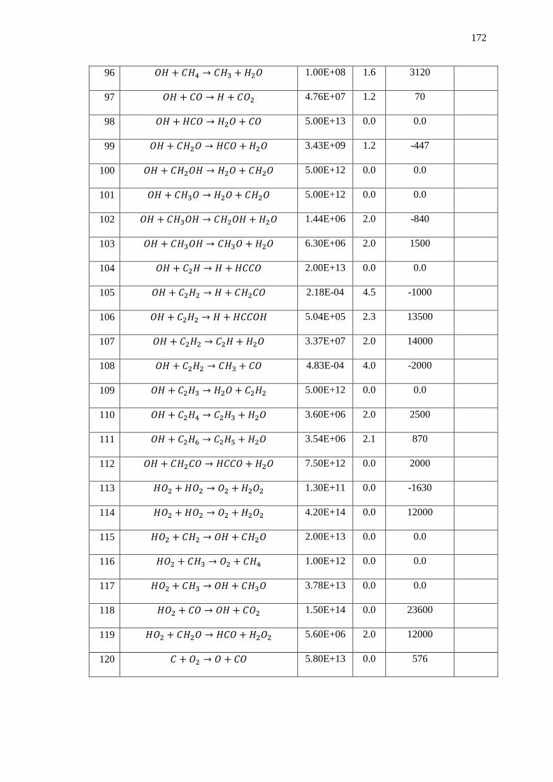
172
96 𝐶𝐶𝐻𝐻 + 𝐶𝐶𝐻𝐻4 → 𝐶𝐶𝐻𝐻3 + 𝐻𝐻2𝐶𝐶 1.00E+08 1.6 3120
97 𝐶𝐶𝐻𝐻 + 𝐶𝐶𝐶𝐶 → 𝐻𝐻 + 𝐶𝐶𝐶𝐶2 4.76E+07 1.2 70
98 𝐶𝐶𝐻𝐻 + 𝐻𝐻𝐶𝐶𝐶𝐶 → 𝐻𝐻2𝐶𝐶 + 𝐶𝐶𝐶𝐶 5.00E+13 0.0 0.0
99 𝐶𝐶𝐻𝐻 + 𝐶𝐶𝐻𝐻2𝐶𝐶 → 𝐻𝐻𝐶𝐶𝐶𝐶 +𝐻𝐻2𝐶𝐶 3.43E+09 1.2 -447
100 𝐶𝐶𝐻𝐻 + 𝐶𝐶𝐻𝐻2𝐶𝐶𝐻𝐻 → 𝐻𝐻2𝐶𝐶 + 𝐶𝐶𝐻𝐻2𝐶𝐶 5.00E+12 0.0 0.0
101 𝐶𝐶𝐻𝐻 + 𝐶𝐶𝐻𝐻3𝐶𝐶 → 𝐻𝐻2𝐶𝐶 + 𝐶𝐶𝐻𝐻2𝐶𝐶 5.00E+12 0.0 0.0
102 𝐶𝐶𝐻𝐻 + 𝐶𝐶𝐻𝐻3𝐶𝐶𝐻𝐻 → 𝐶𝐶𝐻𝐻2𝐶𝐶𝐻𝐻 + 𝐻𝐻2𝐶𝐶 1.44E+06 2.0 -840
103 𝐶𝐶𝐻𝐻 + 𝐶𝐶𝐻𝐻3𝐶𝐶𝐻𝐻 → 𝐶𝐶𝐻𝐻3𝐶𝐶 + 𝐻𝐻2𝐶𝐶 6.30E+06 2.0 1500
104 𝐶𝐶𝐻𝐻 + 𝐶𝐶2𝐻𝐻 → 𝐻𝐻 +𝐻𝐻𝐶𝐶𝐶𝐶𝐶𝐶 2.00E+13 0.0 0.0
105 𝐶𝐶𝐻𝐻 + 𝐶𝐶2𝐻𝐻2 → 𝐻𝐻 + 𝐶𝐶𝐻𝐻2𝐶𝐶𝐶𝐶 2.18E-04 4.5 -1000
106 𝐶𝐶𝐻𝐻 + 𝐶𝐶2𝐻𝐻2 → 𝐻𝐻 + 𝐻𝐻𝐶𝐶𝐶𝐶𝐶𝐶𝐻𝐻 5.04E+05 2.3 13500
107 𝐶𝐶𝐻𝐻 + 𝐶𝐶2𝐻𝐻2 → 𝐶𝐶2𝐻𝐻 + 𝐻𝐻2𝐶𝐶 3.37E+07 2.0 14000
108 𝐶𝐶𝐻𝐻 + 𝐶𝐶2𝐻𝐻2 → 𝐶𝐶𝐻𝐻3 + 𝐶𝐶𝐶𝐶 4.83E-04 4.0 -2000
109 𝐶𝐶𝐻𝐻 + 𝐶𝐶2𝐻𝐻3 → 𝐻𝐻2𝐶𝐶 + 𝐶𝐶2𝐻𝐻2 5.00E+12 0.0 0.0
110 𝐶𝐶𝐻𝐻 + 𝐶𝐶2𝐻𝐻4 → 𝐶𝐶2𝐻𝐻3 + 𝐻𝐻2𝐶𝐶 3.60E+06 2.0 2500
111 𝐶𝐶𝐻𝐻 + 𝐶𝐶2𝐻𝐻6 → 𝐶𝐶2𝐻𝐻5 + 𝐻𝐻2𝐶𝐶 3.54E+06 2.1 870
112 𝐶𝐶𝐻𝐻 + 𝐶𝐶𝐻𝐻2𝐶𝐶𝐶𝐶 → 𝐻𝐻𝐶𝐶𝐶𝐶𝐶𝐶 + 𝐻𝐻2𝐶𝐶 7.50E+12 0.0 2000
113 𝐻𝐻𝐶𝐶2 +𝐻𝐻𝐶𝐶2 → 𝐶𝐶2 +𝐻𝐻2𝐶𝐶2 1.30E+11 0.0 -1630
114 𝐻𝐻𝐶𝐶2 +𝐻𝐻𝐶𝐶2 → 𝐶𝐶2 +𝐻𝐻2𝐶𝐶2 4.20E+14 0.0 12000
115 𝐻𝐻𝐶𝐶2 + 𝐶𝐶𝐻𝐻2 → 𝐶𝐶𝐻𝐻 + 𝐶𝐶𝐻𝐻2𝐶𝐶 2.00E+13 0.0 0.0
116 𝐻𝐻𝐶𝐶2 + 𝐶𝐶𝐻𝐻3 → 𝐶𝐶2 + 𝐶𝐶𝐻𝐻4 1.00E+12 0.0 0.0
117 𝐻𝐻𝐶𝐶2 + 𝐶𝐶𝐻𝐻3 → 𝐶𝐶𝐻𝐻 + 𝐶𝐶𝐻𝐻3𝐶𝐶 3.78E+13 0.0 0.0
118 𝐻𝐻𝐶𝐶2 + 𝐶𝐶𝐶𝐶 → 𝐶𝐶𝐻𝐻 + 𝐶𝐶𝐶𝐶2 1.50E+14 0.0 23600
119 𝐻𝐻𝐶𝐶2 + 𝐶𝐶𝐻𝐻2𝐶𝐶 → 𝐻𝐻𝐶𝐶𝐶𝐶 + 𝐻𝐻2𝐶𝐶2 5.60E+06 2.0 12000
120 𝐶𝐶 + 𝐶𝐶2 → 𝐶𝐶 + 𝐶𝐶𝐶𝐶 5.80E+13 0.0 576
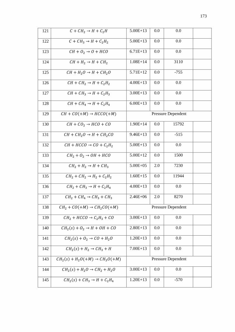
173
121 𝐶𝐶 + 𝐶𝐶𝐻𝐻2 → 𝐻𝐻 + 𝐶𝐶2𝐻𝐻 5.00E+13 0.0 0.0
122 𝐶𝐶 + 𝐶𝐶𝐻𝐻3 → 𝐻𝐻 + 𝐶𝐶2𝐻𝐻2 5.00E+13 0.0 0.0
123 𝐶𝐶𝐻𝐻 + 𝐶𝐶2 → 𝐶𝐶 + 𝐻𝐻𝐶𝐶𝐶𝐶 6.71E+13 0.0 0.0
124 𝐶𝐶𝐻𝐻 + 𝐻𝐻2 → 𝐻𝐻 + 𝐶𝐶𝐻𝐻2 1.08E+14 0.0 3110
125 𝐶𝐶𝐻𝐻 + 𝐻𝐻2𝐶𝐶 → 𝐻𝐻 + 𝐶𝐶𝐻𝐻2𝐶𝐶 5.71E+12 0.0 -755
126 𝐶𝐶𝐻𝐻 + 𝐶𝐶𝐻𝐻2 → 𝐻𝐻 + 𝐶𝐶2𝐻𝐻2 4.00E+13 0.0 0.0
127 𝐶𝐶𝐻𝐻 + 𝐶𝐶𝐻𝐻3 → 𝐻𝐻 + 𝐶𝐶2𝐻𝐻3 3.00E+13 0.0 0.0
128 𝐶𝐶𝐻𝐻 + 𝐶𝐶𝐻𝐻4 → 𝐻𝐻 + 𝐶𝐶2𝐻𝐻4 6.00E+13 0.0 0.0
129 𝐶𝐶𝐻𝐻 + 𝐶𝐶𝐶𝐶(+𝑀𝑀) → 𝐻𝐻𝐶𝐶𝐶𝐶𝐶𝐶(+𝑀𝑀) Pressure Dependent
130 𝐶𝐶𝐻𝐻 + 𝐶𝐶𝐶𝐶2 → 𝐻𝐻𝐶𝐶𝐶𝐶 + 𝐶𝐶𝐶𝐶 1.90E+14 0.0 15792
131 𝐶𝐶𝐻𝐻 + 𝐶𝐶𝐻𝐻2𝐶𝐶 → 𝐻𝐻 + 𝐶𝐶𝐻𝐻2𝐶𝐶𝐶𝐶 9.46E+13 0.0 -515
132 𝐶𝐶𝐻𝐻 + 𝐻𝐻𝐶𝐶𝐶𝐶𝐶𝐶 → 𝐶𝐶𝐶𝐶 + 𝐶𝐶2𝐻𝐻2 5.00E+13 0.0 0.0
133 𝐶𝐶𝐻𝐻2 + 𝐶𝐶2 → 𝐶𝐶𝐻𝐻 + 𝐻𝐻𝐶𝐶𝐶𝐶 5.00E+12 0.0 1500
134 𝐶𝐶𝐻𝐻2 + 𝐻𝐻2 → 𝐻𝐻 + 𝐶𝐶𝐻𝐻3 5.00E+05 2.0 7230
135 𝐶𝐶𝐻𝐻2 + 𝐶𝐶𝐻𝐻2 → 𝐻𝐻2 + 𝐶𝐶2𝐻𝐻2 1.60E+15 0.0 11944
136 𝐶𝐶𝐻𝐻2 + 𝐶𝐶𝐻𝐻3 → 𝐻𝐻 + 𝐶𝐶2𝐻𝐻4 4.00E+13 0.0 0.0
137 𝐶𝐶𝐻𝐻2 + 𝐶𝐶𝐻𝐻4 → 𝐶𝐶𝐻𝐻3 + 𝐶𝐶𝐻𝐻3 2.46E+06 2.0 8270
138 𝐶𝐶𝐻𝐻2 + 𝐶𝐶𝐶𝐶(+𝑀𝑀) → 𝐶𝐶𝐻𝐻2𝐶𝐶𝐶𝐶(+𝑀𝑀) Pressure Dependent
139 𝐶𝐶𝐻𝐻2 + 𝐻𝐻𝐶𝐶𝐶𝐶𝐶𝐶 → 𝐶𝐶2𝐻𝐻3 + 𝐶𝐶𝐶𝐶 3.00E+13 0.0 0.0
140 𝐶𝐶𝐻𝐻2(𝑠𝑠) + 𝐶𝐶2 → 𝐻𝐻 + 𝐶𝐶𝐻𝐻 + 𝐶𝐶𝐶𝐶 2.80E+13 0.0 0.0
141 𝐶𝐶𝐻𝐻2(𝑠𝑠) + 𝐶𝐶2 → 𝐶𝐶𝐶𝐶 + 𝐻𝐻2𝐶𝐶 1.20E+13 0.0 0.0
142 𝐶𝐶𝐻𝐻2(𝑠𝑠) + 𝐻𝐻2 → 𝐶𝐶𝐻𝐻3 +𝐻𝐻 7.00E+13 0.0 0.0
143 𝐶𝐶𝐻𝐻2(𝑠𝑠) +𝐻𝐻2𝐶𝐶(+𝑀𝑀) → 𝐶𝐶𝐻𝐻3𝐶𝐶(+𝑀𝑀) Pressure Dependent
144 𝐶𝐶𝐻𝐻2(𝑠𝑠) + 𝐻𝐻2𝐶𝐶 → 𝐶𝐶𝐻𝐻2 + 𝐻𝐻2𝐶𝐶 3.00E+13 0.0 0.0
145 𝐶𝐶𝐻𝐻2(𝑠𝑠) + 𝐶𝐶𝐻𝐻3 → 𝐻𝐻 + 𝐶𝐶2𝐻𝐻4 1.20E+13 0.0 -570
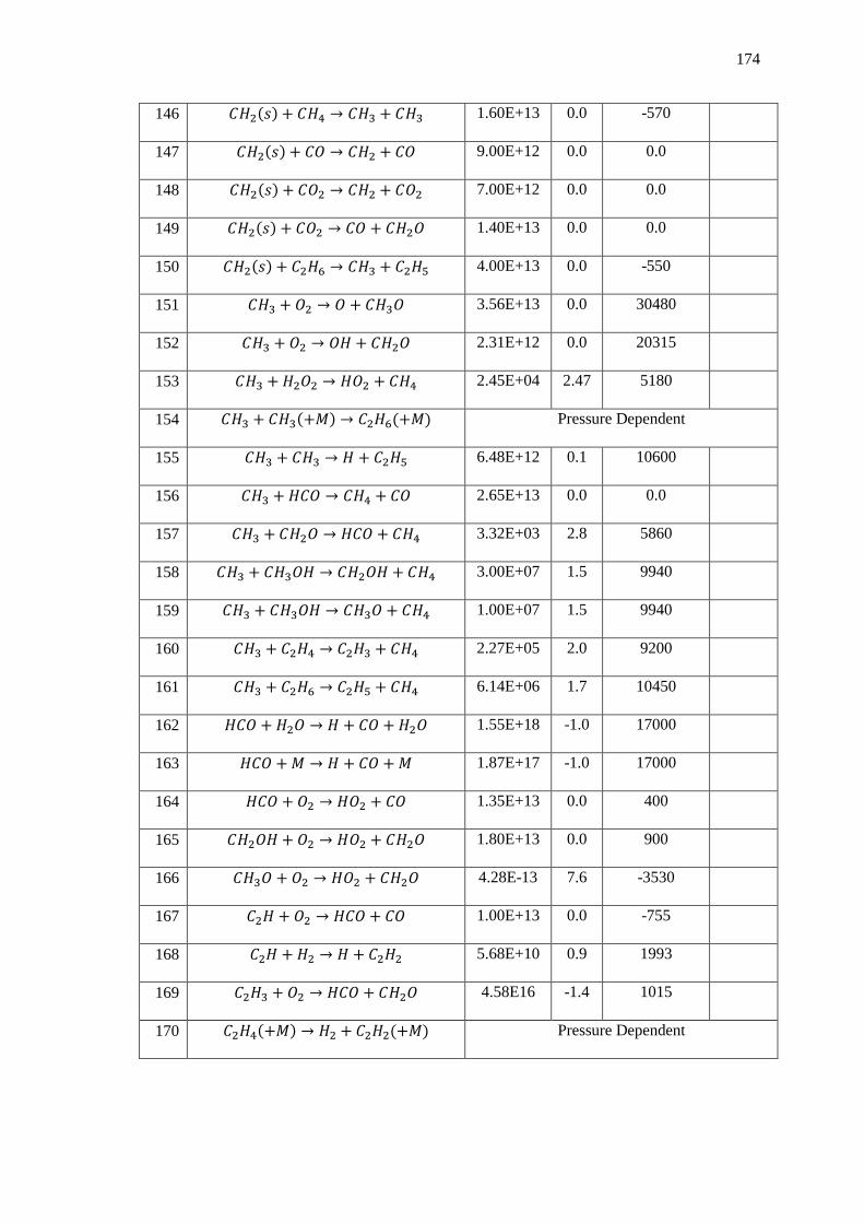
174
146 𝐶𝐶𝐻𝐻2(𝑠𝑠) + 𝐶𝐶𝐻𝐻4 → 𝐶𝐶𝐻𝐻3 + 𝐶𝐶𝐻𝐻3 1.60E+13 0.0 -570
147 𝐶𝐶𝐻𝐻2(𝑠𝑠) + 𝐶𝐶𝐶𝐶 → 𝐶𝐶𝐻𝐻2 + 𝐶𝐶𝐶𝐶 9.00E+12 0.0 0.0
148 𝐶𝐶𝐻𝐻2(𝑠𝑠) + 𝐶𝐶𝐶𝐶2 → 𝐶𝐶𝐻𝐻2 + 𝐶𝐶𝐶𝐶2 7.00E+12 0.0 0.0
149 𝐶𝐶𝐻𝐻2(𝑠𝑠) + 𝐶𝐶𝐶𝐶2 → 𝐶𝐶𝐶𝐶 + 𝐶𝐶𝐻𝐻2𝐶𝐶 1.40E+13 0.0 0.0
150 𝐶𝐶𝐻𝐻2(𝑠𝑠) + 𝐶𝐶2𝐻𝐻6 → 𝐶𝐶𝐻𝐻3 + 𝐶𝐶2𝐻𝐻5 4.00E+13 0.0 -550
151 𝐶𝐶𝐻𝐻3 + 𝐶𝐶2 → 𝐶𝐶 + 𝐶𝐶𝐻𝐻3𝐶𝐶 3.56E+13 0.0 30480
152 𝐶𝐶𝐻𝐻3 + 𝐶𝐶2 → 𝐶𝐶𝐻𝐻 + 𝐶𝐶𝐻𝐻2𝐶𝐶 2.31E+12 0.0 20315
153 𝐶𝐶𝐻𝐻3 + 𝐻𝐻2𝐶𝐶2 → 𝐻𝐻𝐶𝐶2 + 𝐶𝐶𝐻𝐻4 2.45E+04 2.47 5180
154 𝐶𝐶𝐻𝐻3 + 𝐶𝐶𝐻𝐻3(+𝑀𝑀) → 𝐶𝐶2𝐻𝐻6(+𝑀𝑀) Pressure Dependent
155 𝐶𝐶𝐻𝐻3 + 𝐶𝐶𝐻𝐻3 → 𝐻𝐻 + 𝐶𝐶2𝐻𝐻5 6.48E+12 0.1 10600
156 𝐶𝐶𝐻𝐻3 + 𝐻𝐻𝐶𝐶𝐶𝐶 → 𝐶𝐶𝐻𝐻4 + 𝐶𝐶𝐶𝐶 2.65E+13 0.0 0.0
157 𝐶𝐶𝐻𝐻3 + 𝐶𝐶𝐻𝐻2𝐶𝐶 → 𝐻𝐻𝐶𝐶𝐶𝐶 + 𝐶𝐶𝐻𝐻4 3.32E+03 2.8 5860
158 𝐶𝐶𝐻𝐻3 + 𝐶𝐶𝐻𝐻3𝐶𝐶𝐻𝐻 → 𝐶𝐶𝐻𝐻2𝐶𝐶𝐻𝐻 + 𝐶𝐶𝐻𝐻4 3.00E+07 1.5 9940
159 𝐶𝐶𝐻𝐻3 + 𝐶𝐶𝐻𝐻3𝐶𝐶𝐻𝐻 → 𝐶𝐶𝐻𝐻3𝐶𝐶 + 𝐶𝐶𝐻𝐻4 1.00E+07 1.5 9940
160 𝐶𝐶𝐻𝐻3 + 𝐶𝐶2𝐻𝐻4 → 𝐶𝐶2𝐻𝐻3 + 𝐶𝐶𝐻𝐻4 2.27E+05 2.0 9200
161 𝐶𝐶𝐻𝐻3 + 𝐶𝐶2𝐻𝐻6 → 𝐶𝐶2𝐻𝐻5 + 𝐶𝐶𝐻𝐻4 6.14E+06 1.7 10450
162 𝐻𝐻𝐶𝐶𝐶𝐶 + 𝐻𝐻2𝐶𝐶 → 𝐻𝐻 + 𝐶𝐶𝐶𝐶 + 𝐻𝐻2𝐶𝐶 1.55E+18 -1.0 17000
163 𝐻𝐻𝐶𝐶𝐶𝐶 +𝑀𝑀 → 𝐻𝐻 + 𝐶𝐶𝐶𝐶 + 𝑀𝑀 1.87E+17 -1.0 17000
164 𝐻𝐻𝐶𝐶𝐶𝐶 + 𝐶𝐶2 → 𝐻𝐻𝐶𝐶2 + 𝐶𝐶𝐶𝐶 1.35E+13 0.0 400
165 𝐶𝐶𝐻𝐻2𝐶𝐶𝐻𝐻 + 𝐶𝐶2 → 𝐻𝐻𝐶𝐶2 + 𝐶𝐶𝐻𝐻2𝐶𝐶 1.80E+13 0.0 900
166 𝐶𝐶𝐻𝐻3𝐶𝐶 + 𝐶𝐶2 → 𝐻𝐻𝐶𝐶2 + 𝐶𝐶𝐻𝐻2𝐶𝐶 4.28E-13 7.6 -3530
167 𝐶𝐶2𝐻𝐻 + 𝐶𝐶2 → 𝐻𝐻𝐶𝐶𝐶𝐶 + 𝐶𝐶𝐶𝐶 1.00E+13 0.0 -755
168 𝐶𝐶2𝐻𝐻 + 𝐻𝐻2 → 𝐻𝐻 + 𝐶𝐶2𝐻𝐻2 5.68E+10 0.9 1993
169 𝐶𝐶2𝐻𝐻3 + 𝐶𝐶2 → 𝐻𝐻𝐶𝐶𝐶𝐶 + 𝐶𝐶𝐻𝐻2𝐶𝐶 4.58E16 -1.4 1015
170 𝐶𝐶2𝐻𝐻4(+𝑀𝑀) → 𝐻𝐻2 + 𝐶𝐶2𝐻𝐻2(+𝑀𝑀) Pressure Dependent
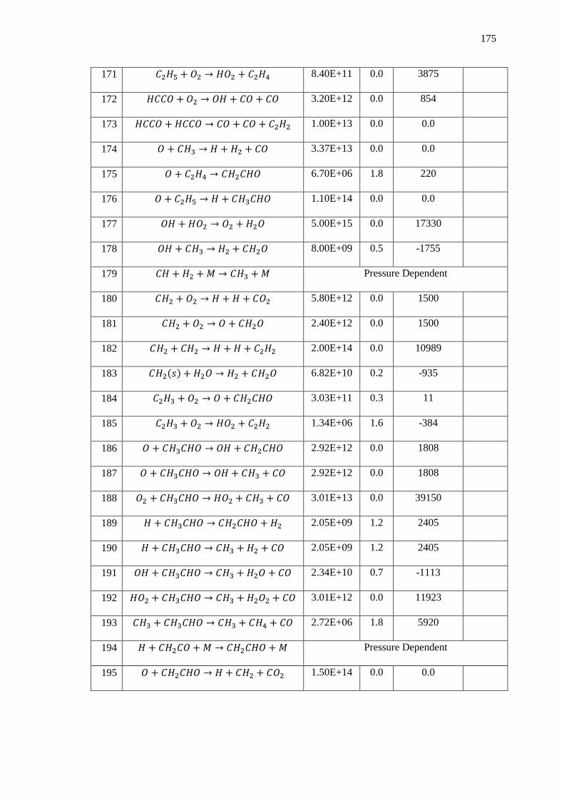
175
171 𝐶𝐶2𝐻𝐻5 + 𝐶𝐶2 → 𝐻𝐻𝐶𝐶2 + 𝐶𝐶2𝐻𝐻4 8.40E+11 0.0 3875
172 𝐻𝐻𝐶𝐶𝐶𝐶𝐶𝐶 + 𝐶𝐶2 → 𝐶𝐶𝐻𝐻 + 𝐶𝐶𝐶𝐶 + 𝐶𝐶𝐶𝐶 3.20E+12 0.0 854
173 𝐻𝐻𝐶𝐶𝐶𝐶𝐶𝐶 +𝐻𝐻𝐶𝐶𝐶𝐶𝐶𝐶 → 𝐶𝐶𝐶𝐶 + 𝐶𝐶𝐶𝐶 + 𝐶𝐶2𝐻𝐻2 1.00E+13 0.0 0.0
174 𝐶𝐶 + 𝐶𝐶𝐻𝐻3 → 𝐻𝐻 + 𝐻𝐻2 + 𝐶𝐶𝐶𝐶 3.37E+13 0.0 0.0
175 𝐶𝐶 + 𝐶𝐶2𝐻𝐻4 → 𝐶𝐶𝐻𝐻2𝐶𝐶𝐻𝐻𝐶𝐶 6.70E+06 1.8 220
176 𝐶𝐶 + 𝐶𝐶2𝐻𝐻5 → 𝐻𝐻 + 𝐶𝐶𝐻𝐻3𝐶𝐶𝐻𝐻𝐶𝐶 1.10E+14 0.0 0.0
177 𝐶𝐶𝐻𝐻 + 𝐻𝐻𝐶𝐶2 → 𝐶𝐶2 +𝐻𝐻2𝐶𝐶 5.00E+15 0.0 17330
178 𝐶𝐶𝐻𝐻 + 𝐶𝐶𝐻𝐻3 → 𝐻𝐻2 + 𝐶𝐶𝐻𝐻2𝐶𝐶 8.00E+09 0.5 -1755
179 𝐶𝐶𝐻𝐻 + 𝐻𝐻2 + 𝑀𝑀 → 𝐶𝐶𝐻𝐻3 +𝑀𝑀 Pressure Dependent
180 𝐶𝐶𝐻𝐻2 + 𝐶𝐶2 → 𝐻𝐻 + 𝐻𝐻 + 𝐶𝐶𝐶𝐶2 5.80E+12 0.0 1500
181 𝐶𝐶𝐻𝐻2 + 𝐶𝐶2 → 𝐶𝐶 + 𝐶𝐶𝐻𝐻2𝐶𝐶 2.40E+12 0.0 1500
182 𝐶𝐶𝐻𝐻2 + 𝐶𝐶𝐻𝐻2 → 𝐻𝐻 + 𝐻𝐻 + 𝐶𝐶2𝐻𝐻2 2.00E+14 0.0 10989
183 𝐶𝐶𝐻𝐻2(𝑠𝑠) + 𝐻𝐻2𝐶𝐶 → 𝐻𝐻2 + 𝐶𝐶𝐻𝐻2𝐶𝐶 6.82E+10 0.2 -935
184 𝐶𝐶2𝐻𝐻3 + 𝐶𝐶2 → 𝐶𝐶 + 𝐶𝐶𝐻𝐻2𝐶𝐶𝐻𝐻𝐶𝐶 3.03E+11 0.3 11
185 𝐶𝐶2𝐻𝐻3 + 𝐶𝐶2 → 𝐻𝐻𝐶𝐶2 + 𝐶𝐶2𝐻𝐻2 1.34E+06 1.6 -384
186 𝐶𝐶 + 𝐶𝐶𝐻𝐻3𝐶𝐶𝐻𝐻𝐶𝐶 → 𝐶𝐶𝐻𝐻 + 𝐶𝐶𝐻𝐻2𝐶𝐶𝐻𝐻𝐶𝐶 2.92E+12 0.0 1808
187 𝐶𝐶 + 𝐶𝐶𝐻𝐻3𝐶𝐶𝐻𝐻𝐶𝐶 → 𝐶𝐶𝐻𝐻 + 𝐶𝐶𝐻𝐻3 + 𝐶𝐶𝐶𝐶 2.92E+12 0.0 1808
188 𝐶𝐶2 + 𝐶𝐶𝐻𝐻3𝐶𝐶𝐻𝐻𝐶𝐶 → 𝐻𝐻𝐶𝐶2 + 𝐶𝐶𝐻𝐻3 + 𝐶𝐶𝐶𝐶 3.01E+13 0.0 39150
189 𝐻𝐻 + 𝐶𝐶𝐻𝐻3𝐶𝐶𝐻𝐻𝐶𝐶 → 𝐶𝐶𝐻𝐻2𝐶𝐶𝐻𝐻𝐶𝐶 + 𝐻𝐻2 2.05E+09 1.2 2405
190 𝐻𝐻 + 𝐶𝐶𝐻𝐻3𝐶𝐶𝐻𝐻𝐶𝐶 → 𝐶𝐶𝐻𝐻3 + 𝐻𝐻2 + 𝐶𝐶𝐶𝐶 2.05E+09 1.2 2405
191 𝐶𝐶𝐻𝐻 + 𝐶𝐶𝐻𝐻3𝐶𝐶𝐻𝐻𝐶𝐶 → 𝐶𝐶𝐻𝐻3 + 𝐻𝐻2𝐶𝐶 + 𝐶𝐶𝐶𝐶 2.34E+10 0.7 -1113
192 𝐻𝐻𝐶𝐶2 + 𝐶𝐶𝐻𝐻3𝐶𝐶𝐻𝐻𝐶𝐶 → 𝐶𝐶𝐻𝐻3 + 𝐻𝐻2𝐶𝐶2 + 𝐶𝐶𝐶𝐶 3.01E+12 0.0 11923
193 𝐶𝐶𝐻𝐻3 + 𝐶𝐶𝐻𝐻3𝐶𝐶𝐻𝐻𝐶𝐶 → 𝐶𝐶𝐻𝐻3 + 𝐶𝐶𝐻𝐻4 + 𝐶𝐶𝐶𝐶 2.72E+06 1.8 5920
194 𝐻𝐻 + 𝐶𝐶𝐻𝐻2𝐶𝐶𝐶𝐶 + 𝑀𝑀 → 𝐶𝐶𝐻𝐻2𝐶𝐶𝐻𝐻𝐶𝐶 + 𝑀𝑀 Pressure Dependent
195 𝐶𝐶 + 𝐶𝐶𝐻𝐻2𝐶𝐶𝐻𝐻𝐶𝐶 → 𝐻𝐻 + 𝐶𝐶𝐻𝐻2 + 𝐶𝐶𝐶𝐶2 1.50E+14 0.0 0.0

176
196 𝐶𝐶2 + 𝐶𝐶𝐻𝐻2𝐶𝐶𝐻𝐻𝐶𝐶 → 𝐶𝐶𝐻𝐻 + 𝐶𝐶𝐶𝐶 + 𝐶𝐶𝐻𝐻2𝐶𝐶 1.81E+10 0.0 0.0
197 𝐶𝐶2 + 𝐶𝐶𝐻𝐻2𝐶𝐶𝐻𝐻𝐶𝐶 → 𝐶𝐶𝐻𝐻 + 𝐻𝐻𝐶𝐶𝐶𝐶 + 𝐻𝐻𝐶𝐶𝐶𝐶 2.35E+10 0.0 0.0
198 𝐻𝐻 + 𝐶𝐶𝐻𝐻2𝐶𝐶𝐻𝐻𝐶𝐶 → 𝐶𝐶𝐻𝐻3 + 𝐻𝐻𝐶𝐶𝐶𝐶 2.20E+13 0.0 0.0
199 𝐻𝐻 + 𝐶𝐶𝐻𝐻2𝐶𝐶𝐻𝐻𝐶𝐶 → 𝐶𝐶𝐻𝐻2𝐶𝐶𝐶𝐶 + 𝐻𝐻2 1.10E+13 0.0 0.0
200 𝐶𝐶𝐻𝐻 + 𝐶𝐶𝐻𝐻2𝐶𝐶𝐻𝐻𝐶𝐶 → 𝐻𝐻2𝐶𝐶 + 𝐶𝐶𝐻𝐻2𝐶𝐶𝐶𝐶 1.20E+13 0.0 0.0
201 𝐶𝐶𝐻𝐻 + 𝐶𝐶𝐻𝐻2𝐶𝐶𝐻𝐻𝐶𝐶 → 𝐻𝐻𝐶𝐶𝐶𝐶 + 𝐶𝐶𝐻𝐻2𝐶𝐶𝐻𝐻 3.01E+13 0.0 0.0
202 𝐶𝐶𝐻𝐻3 + 𝐶𝐶2𝐻𝐻5 + 𝑀𝑀 → 𝐶𝐶3𝐻𝐻8 + 𝑀𝑀 Pressure Dependent
203 𝐶𝐶 + 𝐶𝐶3𝐻𝐻8 → 𝐶𝐶𝐻𝐻 + 𝐶𝐶3𝐻𝐻7 1.93E+05 2.7 3716
204 𝐻𝐻 + 𝐶𝐶3𝐻𝐻8 → 𝐶𝐶3𝐻𝐻7 + 𝐻𝐻2 1.32E+06 2.5 6756
205 𝐶𝐶𝐻𝐻 + 𝐶𝐶3𝐻𝐻8 → 𝐶𝐶3𝐻𝐻7 + 𝐻𝐻2 3.16E+07 1.8 934
206 𝐶𝐶3𝐻𝐻7 + 𝐻𝐻2𝐶𝐶2 → 𝐻𝐻𝐶𝐶2 + 𝐶𝐶3𝐻𝐻8 3.78E+02 2.7 1500
207 𝐶𝐶𝐻𝐻3 + 𝐶𝐶3𝐻𝐻8 → 𝐶𝐶3𝐻𝐻7 + 𝐶𝐶𝐻𝐻4 9.03E-01 3.6 7154
208 𝐶𝐶𝐻𝐻3 + 𝐶𝐶2𝐻𝐻4 + 𝑀𝑀 → 𝐶𝐶3𝐻𝐻7 + 𝑀𝑀 Pressure Dependent
209 𝐶𝐶 + 𝐶𝐶3𝐻𝐻7 → 𝐶𝐶2𝐻𝐻5 + 𝐶𝐶𝐻𝐻2𝐶𝐶 9.64E+13 0.0 0.0
210 𝐻𝐻 + 𝐶𝐶3𝐻𝐻7 + 𝑀𝑀 → 𝐶𝐶3𝐻𝐻8 +𝑀𝑀 Pressure Dependent
211 𝐻𝐻 + 𝐶𝐶3𝐻𝐻7 → 𝐶𝐶𝐻𝐻3 + 𝐶𝐶2𝐻𝐻5 4.06E+06 2.2 890
212 𝐶𝐶𝐻𝐻 + 𝐶𝐶3𝐻𝐻7 → 𝐶𝐶2𝐻𝐻5 + 𝐶𝐶𝐻𝐻2𝐶𝐶𝐻𝐻 2.41E+13 0.0 0.0
213 𝐻𝐻𝐶𝐶2 + 𝐶𝐶3𝐻𝐻7 → 𝐶𝐶2 + 𝐶𝐶3𝐻𝐻8 2.55E+10 0.3 -943
214 𝐻𝐻𝐶𝐶2 + 𝐶𝐶3𝐻𝐻7 → 𝐶𝐶𝐻𝐻 + 𝐶𝐶2𝐻𝐻5 + 𝐶𝐶𝐻𝐻2𝐶𝐶 2.41E+13 0.0 0.0
215 𝐶𝐶𝐻𝐻3 + 𝐶𝐶3𝐻𝐻7 → 𝐶𝐶2𝐻𝐻5 + 𝐶𝐶2𝐻𝐻5 1.93E+13 -0.3 0.0

177
2. Chemiluminescence Augmentation to GRI Mech 3.0
No. Reaction
Forward Rate Coefficient (Equation 145)
Ref. A b 𝐸𝐸 (kJ/mol)
216 𝐻𝐻 + 𝐶𝐶 + 𝑀𝑀 → 𝐶𝐶𝐻𝐻∗ + 𝑀𝑀 1.50E+13 0.0 25.0 [19]
217 𝐶𝐶𝐻𝐻 + 𝐶𝐶2 → 𝐶𝐶𝐻𝐻∗ + 𝐶𝐶𝐶𝐶 1.80E+11 0.0 0.0 [16]
218 𝐶𝐶𝐻𝐻∗ → 𝐶𝐶𝐻𝐻 + ℎ𝜈𝜈 1.45E+06 0.0 0.0 [14]
219 𝐶𝐶𝐻𝐻∗ + 𝐶𝐶2 → 𝐶𝐶𝐻𝐻 + 𝐶𝐶2 2.10E+12 0.5 -2.02 [14]
220 𝐶𝐶𝐻𝐻∗ + 𝐻𝐻2𝐶𝐶 → 𝐶𝐶𝐻𝐻 + 𝐻𝐻2𝐶𝐶 5.93E+12 .5 -3.61 [14]
221 𝐶𝐶𝐻𝐻∗ + 𝐻𝐻2 → 𝐶𝐶𝐻𝐻 + 𝐻𝐻2 2.95E+12 0.5 -1.86 [14]
222 𝐶𝐶𝐻𝐻∗ + 𝐶𝐶𝐶𝐶2 → 𝐶𝐶𝐻𝐻 + 𝐶𝐶𝐶𝐶2 2.76E+12 0.5 -4.06 [14]
223 𝐶𝐶𝐻𝐻∗ + 𝐶𝐶𝐶𝐶 → 𝐶𝐶𝐻𝐻 + 𝐶𝐶𝐶𝐶 3.23E+12 0.5 -3.3 [14]
224 𝐶𝐶𝐻𝐻∗ + 𝐶𝐶𝐻𝐻4 → 𝐶𝐶𝐻𝐻 + 𝐶𝐶𝐻𝐻4 3.36E+12 0.5 -2.66 [14]
225 𝐶𝐶𝐻𝐻∗ + 𝐶𝐶𝐻𝐻 → 𝐶𝐶𝐻𝐻 + 𝐶𝐶𝐻𝐻 6.01E+12 0.5 -3.19 [14]
226 𝐶𝐶𝐻𝐻∗ + 𝐻𝐻 → 𝐶𝐶𝐻𝐻 + 𝐻𝐻 1.31E+13 0.5 -0.7 [14]
227 𝐶𝐶2𝐻𝐻 + 𝐶𝐶2 → 𝐶𝐶𝐻𝐻(𝐴𝐴) + 𝐶𝐶𝐶𝐶2 3.20E+11 0.0 6.7 [18]
228 𝐶𝐶2𝐻𝐻 + 𝐶𝐶 → 𝐶𝐶𝐻𝐻(𝐴𝐴) + 𝐶𝐶𝐶𝐶 2.50E+12 0.0 0.0 [18]
229 𝐶𝐶2 + 𝐶𝐶𝐻𝐻 → 𝐶𝐶𝐻𝐻(𝐴𝐴) + 𝐶𝐶𝐶𝐶 1.11E+13 0.0 0.0 [16]
230 𝐶𝐶 + 𝐻𝐻 +𝑀𝑀 → 𝐶𝐶𝐻𝐻(𝐴𝐴) + 𝑀𝑀 3.63E+13 0.0 0.0 [16]
231 𝐶𝐶𝐻𝐻(𝐴𝐴) → 𝐶𝐶𝐻𝐻 + ℎ𝜈𝜈 1.86E+06 0.0 0.0 [16]
232 𝐶𝐶𝐻𝐻(𝐴𝐴) + 𝐶𝐶2 → 𝐶𝐶𝐻𝐻 + 𝐶𝐶2 2.48E+06 2.14 -7.2 [14]
233 𝐶𝐶𝐻𝐻(𝐴𝐴) + 𝐻𝐻2𝐶𝐶 → 𝐶𝐶𝐻𝐻 + 𝐻𝐻2𝐶𝐶 5.30E+13 0.0 0.0 [14]
234 𝐶𝐶𝐻𝐻(𝐴𝐴) +𝐻𝐻2 → 𝐶𝐶𝐻𝐻 + 𝐻𝐻2 1.47E+14 0.5 5.7 [14]
235 𝐶𝐶𝐻𝐻(𝐴𝐴) + 𝐶𝐶𝐶𝐶2 → 𝐶𝐶𝐻𝐻 + 𝐶𝐶𝐶𝐶2 2.40E-01 4.3 -7.1 [14]
236 𝐶𝐶𝐻𝐻(𝐴𝐴) + 𝐶𝐶𝐶𝐶 → 𝐶𝐶𝐻𝐻 + 𝐶𝐶𝐶𝐶 2.44E+12 0.5 0.0 [14]
237 𝐶𝐶𝐻𝐻(𝐴𝐴) + 𝐶𝐶𝐻𝐻4 → 𝐶𝐶𝐻𝐻 + 𝐶𝐶𝐻𝐻4 1.73E+13 0.0 0.7 [14]

178
238 𝐶𝐶𝐻𝐻(𝐴𝐴) + 𝐶𝐶𝐻𝐻 → 𝐶𝐶𝐻𝐻 + 𝐶𝐶𝐻𝐻 7.13E+13 0.0 5.7 [14]
239 𝐶𝐶𝐻𝐻(𝐴𝐴) + 𝐻𝐻 → 𝐶𝐶𝐻𝐻 + 𝐻𝐻 2.01E+14 0.0 5.7 [14]
240 𝐶𝐶𝐻𝐻2 + 𝐶𝐶 → 𝐶𝐶2∗ + 𝐻𝐻2 2.40E+12 0.0 0.0 [20]
241 𝐶𝐶3 + 𝐶𝐶 → 𝐶𝐶2∗ + 𝐻𝐻2 4.22E+12 0.0 0.0 [20]
242 𝐶𝐶2∗ → 𝐶𝐶2 + ℎ𝜈𝜈 1.00E+07 0.0 0.0 [20]
243 𝐶𝐶2∗ + 𝑀𝑀 → 𝐶𝐶2 +𝑀𝑀 4.80E+13 0.0 0.0 [20]
244 𝐶𝐶𝐶𝐶 + 𝐶𝐶 → 𝐶𝐶𝐶𝐶2 + ℎ𝜈𝜈 6.8(±0.6)E+05 0.0 1.96 [21]
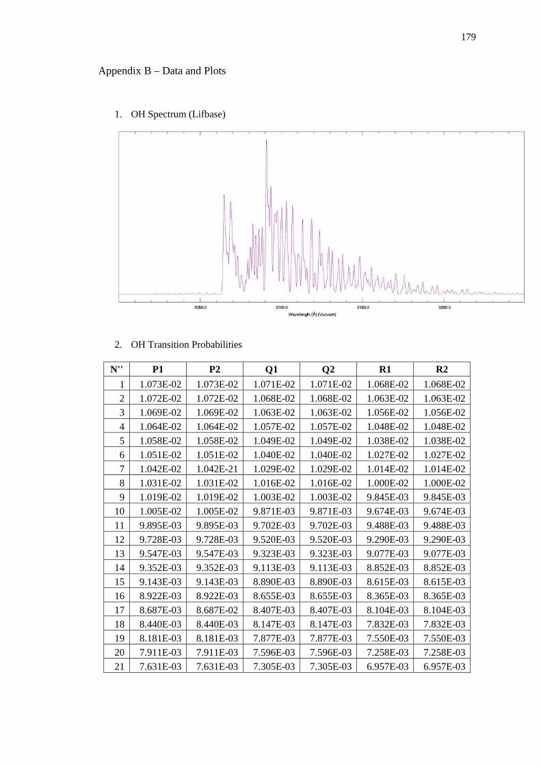
179
Appendix B – Data and Plots
1. OH Spectrum (Lifbase)
2. OH Transition Probabilities
N'' P1 P2 Q1 Q2 R1 R2 1 1.073E-02 1.073E-02 1.071E-02 1.071E-02 1.068E-02 1.068E-02 2 1.072E-02 1.072E-02 1.068E-02 1.068E-02 1.063E-02 1.063E-02 3 1.069E-02 1.069E-02 1.063E-02 1.063E-02 1.056E-02 1.056E-02 4 1.064E-02 1.064E-02 1.057E-02 1.057E-02 1.048E-02 1.048E-02 5 1.058E-02 1.058E-02 1.049E-02 1.049E-02 1.038E-02 1.038E-02 6 1.051E-02 1.051E-02 1.040E-02 1.040E-02 1.027E-02 1.027E-02 7 1.042E-02 1.042E-21 1.029E-02 1.029E-02 1.014E-02 1.014E-02 8 1.031E-02 1.031E-02 1.016E-02 1.016E-02 1.000E-02 1.000E-02 9 1.019E-02 1.019E-02 1.003E-02 1.003E-02 9.845E-03 9.845E-03
10 1.005E-02 1.005E-02 9.871E-03 9.871E-03 9.674E-03 9.674E-03 11 9.895E-03 9.895E-03 9.702E-03 9.702E-03 9.488E-03 9.488E-03 12 9.728E-03 9.728E-03 9.520E-03 9.520E-03 9.290E-03 9.290E-03 13 9.547E-03 9.547E-03 9.323E-03 9.323E-03 9.077E-03 9.077E-03 14 9.352E-03 9.352E-03 9.113E-03 9.113E-03 8.852E-03 8.852E-03 15 9.143E-03 9.143E-03 8.890E-03 8.890E-03 8.615E-03 8.615E-03 16 8.922E-03 8.922E-03 8.655E-03 8.655E-03 8.365E-03 8.365E-03 17 8.687E-03 8.687E-02 8.407E-03 8.407E-03 8.104E-03 8.104E-03 18 8.440E-03 8.440E-03 8.147E-03 8.147E-03 7.832E-03 7.832E-03 19 8.181E-03 8.181E-03 7.877E-03 7.877E-03 7.550E-03 7.550E-03 20 7.911E-03 7.911E-03 7.596E-03 7.596E-03 7.258E-03 7.258E-03 21 7.631E-03 7.631E-03 7.305E-03 7.305E-03 6.957E-03 6.957E-03

180
22 7.340E-03 7.340E-03 7.005E-03 7.005E-03 6.648E-03 6.648E-03 23 7.040E-03 7.040E-03 6.697E-03 6.697E-03 6.332E-03 6.332E-03 24 6.731E-03 6.731E-03 6.380E-03 6.380E-03 6.009E-03 6.009E-03 25 6.415E-03 6.415E-03 6.058E-03 6.058E-03 5.680E-03 5.680E-03 26 6.091E-03 6.091E-03 5.729E-03 5.729E-03 5.347E-03 5.347E-03 27 5.761E-03 5.761E-03 5.395E-03 5.395E-03 5.011E-03 5.011E-03 28 5.426E-03 5.426E-03 5.057E-03 5.057E-03 4.672E-03 4.672E-03 29 5.087E-03 5.087E-03 4.717E-03 4.717E-03 4.331E-03 4.331E-03 30 4.745E-03 4.745E-03 4.375E-03 4.375E-03 3.991E-03 3.991E-03 31 4.401E-03 4.401E-03 4.032E-03 4.032E-03 3.652E-03 3.652E-03 32 4.056E-03 4.056E-03 3.690E-03 3.690E-03 3.315E-03 3.315E-03 33 3.711E-03 3.711E-03 3.350E-03 3.350E-03 2.982E-03 2.982E-03 34 3.369E-03 3.369E-03 3.014E-03 3.014E-03 2.656E-03 2.656E-03 35 3.030E-03 3.030E-03 2.683E-03 2.683E-03 2.337E-03 2.337E-03 36 2.660E-03 2.696E-03 2.360E-03 2.360E-03 2.027E-03 2.027E-03 37 2.369E-03 2.369E-03 2.047E-03 2.047E-03 1.730E-03 1.730E-03 38 2.052E-03 2.052E-03 1.745E-03 1.745E-03 1.447E-03 1.447E-03 39 1.746E-03 1.746E-03 1.457E-03 1.457E-03 1.182E-03 1.182E-03 40 1.455E-03 1.455E-03 1.187E-03 1.187E-03 9.358E-04 9.358E-04
N'' O12 Q12 P12 R21 Q21 S21 1 0.000E+00 1.071E-02 1.073E-02 1.068E-02 1.071E-02 1.062E-02 2 1.074E-02 1.068E-02 1.072E-02 1.063E-02 1.068E-02 1.055E-02 3 1.073E-02 1.063E-02 1.069E-02 1.056E-02 1.063E-02 1.047E-02 4 1.070E-02 1.057E-02 1.064E-02 1.048E-02 1.057E-02 1.037E-02 5 1.066E-02 1.049E-02 1.058E-02 1.038E-02 1.049E-02 1.025E-02 6 1.060E-02 1.040E-02 1.051E-02 1.027E-02 1.040E-02 1.012E-02 7 1.052E-02 1.029E-02 1.042E-21 1.014E-02 1.029E-02 9.977E-03 8 1.043E-02 1.016E-02 1.031E-02 1.000E-02 1.016E-02 9.817E-03 9 1.033E-02 1.003E-02 1.019E-02 9.845E-03 1.003E-02 9.643E-03
10 1.020E-02 9.871E-03 1.005E-02 9.674E-03 9.871E-03 9.455E-03 11 1.007E-02 9.702E-03 9.895E-03 9.488E-03 9.702E-03 9.253E-03 12 9.916E-03 9.520E-03 9.728E-03 9.290E-03 9.520E-03 9.037E-03 13 9.749E-03 9.323E-03 9.547E-03 9.077E-03 9.323E-03 8.809E-03 14 9.569E-03 9.113E-03 9.352E-03 8.852E-03 9.113E-03 8.569E-03 15 9.374E-03 8.890E-03 9.143E-03 8.615E-03 8.890E-03 8.316E-03 16 9.166E-03 8.655E-03 8.922E-03 8.365E-03 8.655E-03 8.053E-03 17 8.944E-03 8.407E-03 8.687E-02 8.104E-03 8.407E-03 7.778E-03 18 8.710E-03 8.147E-03 8.440E-03 7.832E-03 8.147E-03 7.494E-03 19 8.462E-03 7.877E-03 8.181E-03 7.550E-03 7.877E-03 7.200E-03 20 8.203E-03 7.596E-03 7.911E-03 7.258E-03 7.596E-03 6.898E-03 21 7.933E-03 7.305E-03 7.631E-03 6.957E-03 7.305E-03 6.588E-03

181
22 7.652E-03 7.005E-03 7.340E-03 6.648E-03 7.005E-03 2.700E-04 23 7.360E-03 6.697E-03 7.040E-03 6.332E-03 6.697E-03 5.947E-03 24 7.059E-03 6.380E-03 6.731E-03 6.009E-03 6.380E-03 5.619E-03 25 6.750E-03 6.058E-03 6.415E-03 5.680E-03 6.058E-03 5.286E-03 26 6.432E-03 5.729E-03 6.091E-03 5.347E-03 5.729E-03 4.950E-03 27 6.107E-03 5.395E-03 5.761E-03 5.011E-03 5.395E-03 4.613E-03 28 5.776E-03 5.057E-03 5.426E-03 4.672E-03 5.057E-03 4.274E-03 29 5.439E-03 4.717E-03 5.087E-03 4.331E-03 4.717E-03 3.936E-03 30 5.098E-03 4.375E-03 4.745E-03 3.991E-03 4.375E-03 3.599E-03 31 4.754E-03 4.032E-03 4.401E-03 3.652E-03 4.032E-03 3.266E-03 32 4.408E-03 3.690E-03 4.056E-03 3.315E-03 3.690E-03 2.937E-03 33 4.061E-03 3.350E-03 3.711E-03 2.982E-03 3.350E-03 2.614E-03 34 3.714E-03 3.014E-03 3.369E-03 2.656E-03 3.014E-03 2.300E-03 35 3.369E-03 2.683E-03 3.030E-03 2.337E-03 2.683E-03 1.996E-03 36 3.027E-03 2.360E-03 2.696E-03 2.027E-03 2.360E-03 1.704E-03 37 2.691E-03 2.047E-03 2.369E-03 1.730E-03 2.047E-03 1.426E-03 38 2.361E-03 1.745E-03 2.052E-03 1.447E-03 1.745E-03 1.166E-03 39 2.041E-03 1.457E-03 1.746E-03 1.182E-03 1.457E-03 9.257E-04 40 1.733E-03 1.187E-03 1.455E-03 9.358E-04 1.187E-03 0.000E+00
3. OH Emission Lines
N'' (cm-1) P1 P2 Q1 Q2 R1 R2
1 32440.58 0.00 32474.56 32347.98 32542.52 32415.51 2 32390.89 32286.52 32458.60 32354.47 32560.48 32455.66 3 32340.59 32252.91 32441.82 32354.64 32577.58 32489.45 4 32289.08 32213.95 32423.59 32349.21 32593.12 32517.54 5 32235.91 32170.29 32403.41 32338.80 32606.56 32540.49 6 32180.76 32122.46 32380.91 32323.87 32617.48 32558.73 7 32123.40 32070.82 32355.84 32304.76 32625.55 32572.52 8 32063.69 32015.63 32327.98 32281.68 32630.54 32582.04 9 32001.50 31957.09 32297.20 32254.77 32632.23 32587.37
10 31936.77 31895.31 32263.38 32224.13 32630.46 32588.55 11 31869.43 31830.39 32226.40 32189.81 32625.08 32585.59 12 31799.44 31762.39 32186.19 32151.84 32615.96 32578.46 13 31726.76 31691.37 32142.66 32110.19 32602.95 32567.10 14 31651.33 31617.32 32095.73 32064.88 32585.93 32551.47 15 31573.13 31540.28 32045.32 32015.86 32564.78 32531.48 16 31492.11 31460.23 31991.36 31963.09 32539.39 32507.05 17 31408.23 31377.15 31933.76 31906.54 32509.61 32478.09 18 31321.43 31291.04 31872.44 31846.13 32475.33 32444.49 19 31231.67 31201.85 31807.31 31781.81 32436.42 32406.15
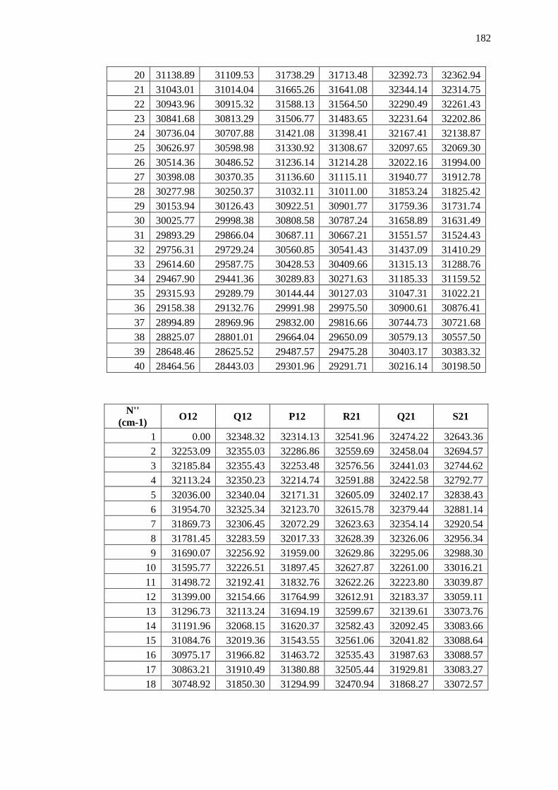
182
N'' (cm-1) O12 Q12 P12 R21 Q21 S21
1 0.00 32348.32 32314.13 32541.96 32474.22 32643.36 2 32253.09 32355.03 32286.86 32559.69 32458.04 32694.57 3 32185.84 32355.43 32253.48 32576.56 32441.03 32744.62 4 32113.24 32350.23 32214.74 32591.88 32422.58 32792.77 5 32036.00 32340.04 32171.31 32605.09 32402.17 32838.43 6 31954.70 32325.34 32123.70 32615.78 32379.44 32881.14 7 31869.73 32306.45 32072.29 32623.63 32354.14 32920.54 8 31781.45 32283.59 32017.33 32628.39 32326.06 32956.34 9 31690.07 32256.92 31959.00 32629.86 32295.06 32988.30
10 31595.77 32226.51 31897.45 32627.87 32261.00 33016.21 11 31498.72 32192.41 31832.76 32622.26 32223.80 33039.87 12 31399.00 32154.66 31764.99 32612.91 32183.37 33059.11 13 31296.73 32113.24 31694.19 32599.67 32139.61 33073.76 14 31191.96 32068.15 31620.37 32582.43 32092.45 33083.66 15 31084.76 32019.36 31543.55 32561.06 32041.82 33088.64 16 30975.17 31966.82 31463.72 32535.43 31987.63 33088.57 17 30863.21 31910.49 31380.88 32505.44 31929.81 33083.27 18 30748.92 31850.30 31294.99 32470.94 31868.27 33072.57
20 31138.89 31109.53 31738.29 31713.48 32392.73 32362.94 21 31043.01 31014.04 31665.26 31641.08 32344.14 32314.75 22 30943.96 30915.32 31588.13 31564.50 32290.49 32261.43 23 30841.68 30813.29 31506.77 31483.65 32231.64 32202.86 24 30736.04 30707.88 31421.08 31398.41 32167.41 32138.87 25 30626.97 30598.98 31330.92 31308.67 32097.65 32069.30 26 30514.36 30486.52 31236.14 31214.28 32022.16 31994.00 27 30398.08 30370.35 31136.60 31115.11 31940.77 31912.78 28 30277.98 30250.37 31032.11 31011.00 31853.24 31825.42 29 30153.94 30126.43 30922.51 30901.77 31759.36 31731.74 30 30025.77 29998.38 30808.58 30787.24 31658.89 31631.49 31 29893.29 29866.04 30687.11 30667.21 31551.57 31524.43 32 29756.31 29729.24 30560.85 30541.43 31437.09 31410.29 33 29614.60 29587.75 30428.53 30409.66 31315.13 31288.76 34 29467.90 29441.36 30289.83 30271.63 31185.33 31159.52 35 29315.93 29289.79 30144.44 30127.03 31047.31 31022.21 36 29158.38 29132.76 29991.98 29975.50 30900.61 30876.41 37 28994.89 28969.96 29832.00 29816.66 30744.73 30721.68 38 28825.07 28801.01 29664.04 29650.09 30579.13 30557.50 39 28648.46 28625.52 29487.57 29475.28 30403.17 30383.32 40 28464.56 28443.03 29301.96 29291.71 30216.14 30198.50

183
19 30632.30 31786.20 31206.02 32431.80 31802.92 33056.33 20 30513.35 31718.10 31113.93 32387.90 31733.67 33034.38 21 30392.06 31645.91 31018.66 32339.10 31660.43 33006.54 22 30268.41 31569.55 30920.15 32285.25 31583.09 32972.65 23 30142.37 31488.90 30818.34 32226.20 31501.53 32932.52 24 30013.89 31403.86 30713.13 32161.79 31415.64 32885.96 25 29882.93 31314.30 30604.43 32091.85 31325.29 32832.78 26 29749.40 31220.08 30492.14 32016.22 31230.35 32772.77 27 29613.25 31121.05 30376.15 31934.71 31130.65 32705.71 28 29474.37 31017.06 30256.31 31847.10 31026.05 32631.36 29 29332.66 30907.91 30132.49 31753.18 30916.37 32549.48 30 29188.00 30793.42 30004.52 31652.74 30801.40 32459.79 31 29040.23 30673.36 29872.22 31545.50 30680.95 32362.00 32 28889.22 30547.49 29735.40 31431.20 30554.78 32255.79 33 28734.77 30415.55 29593.82 31309.54 30422.64 32140.81 34 28576.69 30277.20 29447.24 31180.18 30284.25 32016.67 35 28414.74 30132.17 29295.37 31042.76 30139.29 31882.94 36 28248.67 29980.04 29137.91 30896.87 29987.43 31739.14 37 28078.17 29820.40 28974.51 30742.06 29828.27 31584.75 38 27902.92 29652.75 28804.75 30577.82 29661.37 31419.17 39 27722.53 29476.59 28628.19 30403.59 29486.26 31241.73 40 27536.58 29291.29 28444.34 30218.72 29302.38 31051.67
4. OH Spontaneous Emission Coefficients
N'' (s-1) P1 P2 Q1 Q2 R1 R2
1 8.588E+05 0.000E+00 4.105E+05 4.813E+05 8.072E+04 1.207E+05 2 5.770E+05 3.957E+05 5.156E+05 4.951E+05 1.403E+05 1.703E+05 3 4.949E+05 3.839E+05 5.711E+05 5.435E+05 1.831E+05 2.049E+05 4 4.562E+05 3.823E+05 6.044E+05 5.803E+05 2.138E+05 2.301E+05 5 4.324E+05 3.804E+05 6.243E+05 6.049E+05 2.357E+05 2.484E+05 6 4.151E+05 3.771E+05 6.352E+05 6.200E+05 2.511E+05 2.612E+05 7 4.009E+05 3.721E+05 6.399E+05 6.279E+05 2.617E+05 2.700E+05 8 3.883E+05 3.660E+05 6.398E+05 6.303E+05 2.687E+05 2.756E+05 9 3.767E+05 3.590E+05 6.363E+05 6.285E+05 2.729E+05 2.786E+05
10 3.655E+05 3.512E+05 6.298E+05 6.235E+05 2.748E+05 2.796E+05 11 3.546E+05 3.428E+05 6.210E+05 6.157E+05 2.748E+05 2.789E+05 12 3.438E+05 3.339E+05 6.103E+05 6.057E+05 2.733E+05 2.768E+05 13 3.329E+05 3.245E+05 5.977E+05 5.938E+05 2.704E+05 2.734E+05 14 3.219E+05 3.147E+05 5.837E+05 5.803E+05 2.664E+05 2.689E+05 15 3.108E+05 3.046E+05 5.683E+05 5.654E+05 2.613E+05 2.635E+05 16 2.996E+05 2.942E+05 5.517E+05 5.491E+05 2.553E+05 2.572E+05
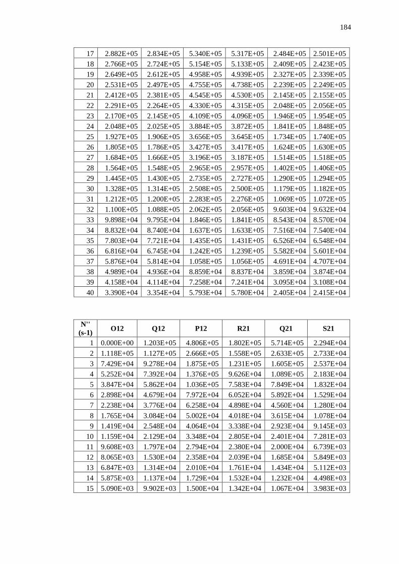
184
17 2.882E+05 2.834E+05 5.340E+05 5.317E+05 2.484E+05 2.501E+05 18 2.766E+05 2.724E+05 5.154E+05 5.133E+05 2.409E+05 2.423E+05 19 2.649E+05 2.612E+05 4.958E+05 4.939E+05 2.327E+05 2.339E+05 20 2.531E+05 2.497E+05 4.755E+05 4.738E+05 2.239E+05 2.249E+05 21 2.412E+05 2.381E+05 4.545E+05 4.530E+05 2.145E+05 2.155E+05 22 2.291E+05 2.264E+05 4.330E+05 4.315E+05 2.048E+05 2.056E+05 23 2.170E+05 2.145E+05 4.109E+05 4.096E+05 1.946E+05 1.954E+05 24 2.048E+05 2.025E+05 3.884E+05 3.872E+05 1.841E+05 1.848E+05 25 1.927E+05 1.906E+05 3.656E+05 3.645E+05 1.734E+05 1.740E+05 26 1.805E+05 1.786E+05 3.427E+05 3.417E+05 1.624E+05 1.630E+05 27 1.684E+05 1.666E+05 3.196E+05 3.187E+05 1.514E+05 1.518E+05 28 1.564E+05 1.548E+05 2.965E+05 2.957E+05 1.402E+05 1.406E+05 29 1.445E+05 1.430E+05 2.735E+05 2.727E+05 1.290E+05 1.294E+05 30 1.328E+05 1.314E+05 2.508E+05 2.500E+05 1.179E+05 1.182E+05 31 1.212E+05 1.200E+05 2.283E+05 2.276E+05 1.069E+05 1.072E+05 32 1.100E+05 1.088E+05 2.062E+05 2.056E+05 9.603E+04 9.632E+04 33 9.898E+04 9.795E+04 1.846E+05 1.841E+05 8.543E+04 8.570E+04 34 8.832E+04 8.740E+04 1.637E+05 1.633E+05 7.516E+04 7.540E+04 35 7.803E+04 7.721E+04 1.435E+05 1.431E+05 6.526E+04 6.548E+04 36 6.816E+04 6.745E+04 1.242E+05 1.239E+05 5.582E+04 5.601E+04 37 5.876E+04 5.814E+04 1.058E+05 1.056E+05 4.691E+04 4.707E+04 38 4.989E+04 4.936E+04 8.859E+04 8.837E+04 3.859E+04 3.874E+04 39 4.158E+04 4.114E+04 7.258E+04 7.241E+04 3.095E+04 3.108E+04 40 3.390E+04 3.354E+04 5.793E+04 5.780E+04 2.405E+04 2.415E+04
N'' (s-1) O12 Q12 P12 R21 Q21 S21
1 0.000E+00 1.203E+05 4.806E+05 1.802E+05 5.714E+05 2.294E+04 2 1.118E+05 1.127E+05 2.666E+05 1.558E+05 2.633E+05 2.733E+04 3 7.429E+04 9.278E+04 1.875E+05 1.231E+05 1.605E+05 2.537E+04 4 5.252E+04 7.392E+04 1.376E+05 9.626E+04 1.089E+05 2.183E+04 5 3.847E+04 5.862E+04 1.036E+05 7.583E+04 7.849E+04 1.832E+04 6 2.898E+04 4.679E+04 7.972E+04 6.052E+04 5.892E+04 1.529E+04 7 2.238E+04 3.776E+04 6.258E+04 4.898E+04 4.560E+04 1.280E+04 8 1.765E+04 3.084E+04 5.002E+04 4.018E+04 3.615E+04 1.078E+04 9 1.419E+04 2.548E+04 4.064E+04 3.338E+04 2.923E+04 9.145E+03
10 1.159E+04 2.129E+04 3.348E+04 2.805E+04 2.401E+04 7.281E+03 11 9.608E+03 1.797E+04 2.794E+04 2.380E+04 2.000E+04 6.739E+03 12 8.065E+03 1.530E+04 2.358E+04 2.039E+04 1.685E+04 5.849E+03 13 6.847E+03 1.314E+04 2.010E+04 1.761E+04 1.434E+04 5.112E+03 14 5.875E+03 1.137E+04 1.729E+04 1.532E+04 1.232E+04 4.498E+03 15 5.090E+03 9.902E+03 1.500E+04 1.342E+04 1.067E+04 3.983E+03

185
16 4.450E+03 8.685E+03 1.311E+04 1.184E+04 9.308E+03 3.549E+03 17 3.927E+03 7.665E+03 1.155E+04 1.051E+04 8.178E+03 3.183E+03 18 3.495E+03 6.806E+03 1.026E+04 9.395E+04 7.234E+03 2.874E+03 19 3.138E+03 6.080E+03 9.171E+03 8.449E+03 6.440E+03 2.611E+03 20 2.843E+03 5.464E+03 8.260E+03 7.646E+03 5.770E+03 2.389E+03 21 2.598E+03 4.940E+03 7.494E+03 6.964E+03 5.201E+03 2.200E+03 22 2.395E+03 4.491E+03 6.848E+03 6.382E+03 4.718E+03 2.040E+03 23 2.226E+03 4.107E+03 6.302E+03 5.885E+03 4.305E+03 1.904E+03 24 2.086E+03 3.776E+03 5.838E+03 5.457E+03 3.950E+03 1.787E+03 25 1.970E+03 3.489E+03 5.442E+03 5.088E+03 3.643E+03 1.688E+03 26 1.873E+03 3.238E+03 5.101E+03 4.765E+03 3.375E+03 1.601E+03 27 1.790E+03 3.016E+03 4.805E+03 4.480E+03 3.140E+03 1.524E+03 28 1.720E+03 2.818E+03 4.544E+03 4.222E+03 2.929E+03 1.454E+03 29 1.658E+03 2.638E+03 4.308E+03 3.985E+03 2.738E+03 1.388E+03 30 1.601E+03 2.470E+03 4.091E+03 3.762E+03 2.562E+03 1.323E+03 31 1.546E+03 2.312E+03 3.884E+03 3.544E+03 2.395E+03 1.258E+03 32 1.492E+03 2.158E+03 3.682E+03 3.328E+03 2.234E+03 1.190E+03 33 1.435E+03 2.007E+03 3.479E+03 3.108E+03 2.075E+03 1.117E+03 34 1.374E+03 1.855E+03 3.271E+03 2.880E+03 1.917E+03 1.039E+03 35 1.308E+03 1.702E+03 3.054E+03 2.643E+03 1.757E+03 9.537E+02 36 1.234E+03 1.544E+03 2.826E+03 2.394E+03 1.594E+03 8.617E+02 37 1.152E+03 1.384E+03 2.585E+03 2.134E+03 1.427E+03 7.632E+02 38 1.061E+03 1.219E+03 2.330E+03 1.865E+03 1.257E+03 6.597E+02 39 9.962E+02 1.053E+03 2.064E+03 1.590E+03 1.085E+03 5.528E+02 40 8.568E+02 8.864E+02 1.789E+03 1.313E+03 9.129E+02 0.000E+00
5. OH Honl London Factors
N'' P1 P2 Q1 Q2 R1 R2 1 1.177 0.000 1.124 0.667 0.331 0.333 2 1.592 0.551 2.127 1.375 0.768 0.706 3 2.063 1.075 3.160 2.274 1.260 1.137 4 2.558 1.619 4.213 3.258 1.776 1.604 5 3.063 2.169 5.270 4.282 2.302 2.092 6 3.572 2.719 6.326 5.321 2.831 2.591 7 4.083 3.265 7.377 6.365 3.359 3.095 8 4.593 3.805 8.423 7.407 3.885 3.601 9 5.102 4.340 9.463 8.446 4.408 4.108
10 5.610 4.870 10.498 9.481 4.929 4.615 11 6.118 5.395 11.528 10.512 5.447 5.121 12 6.624 5.918 12.554 11.539 5.963 5.626 13 7.129 6.437 13.577 12.563 6.477 6.131 14 7.634 6.953 14.596 13.583 6.989 6.636
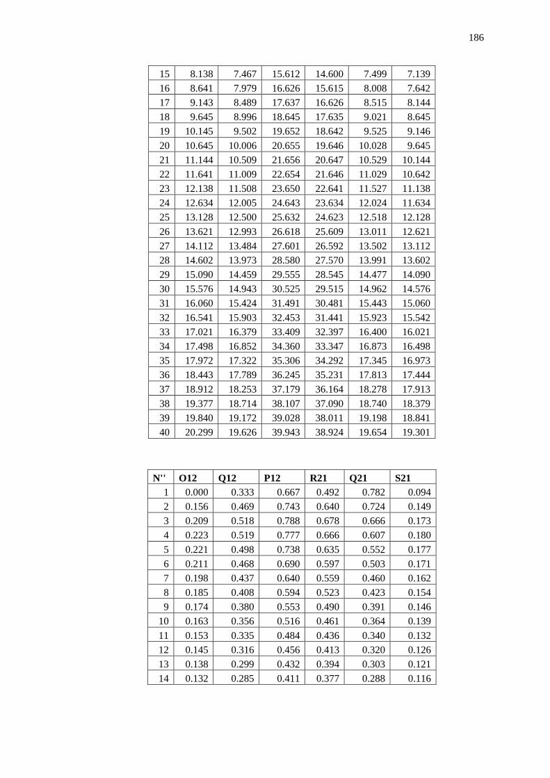
186
15 8.138 7.467 15.612 14.600 7.499 7.139 16 8.641 7.979 16.626 15.615 8.008 7.642 17 9.143 8.489 17.637 16.626 8.515 8.144 18 9.645 8.996 18.645 17.635 9.021 8.645 19 10.145 9.502 19.652 18.642 9.525 9.146 20 10.645 10.006 20.655 19.646 10.028 9.645 21 11.144 10.509 21.656 20.647 10.529 10.144 22 11.641 11.009 22.654 21.646 11.029 10.642 23 12.138 11.508 23.650 22.641 11.527 11.138 24 12.634 12.005 24.643 23.634 12.024 11.634 25 13.128 12.500 25.632 24.623 12.518 12.128 26 13.621 12.993 26.618 25.609 13.011 12.621 27 14.112 13.484 27.601 26.592 13.502 13.112 28 14.602 13.973 28.580 27.570 13.991 13.602 29 15.090 14.459 29.555 28.545 14.477 14.090 30 15.576 14.943 30.525 29.515 14.962 14.576 31 16.060 15.424 31.491 30.481 15.443 15.060 32 16.541 15.903 32.453 31.441 15.923 15.542 33 17.021 16.379 33.409 32.397 16.400 16.021 34 17.498 16.852 34.360 33.347 16.873 16.498 35 17.972 17.322 35.306 34.292 17.345 16.973 36 18.443 17.789 36.245 35.231 17.813 17.444 37 18.912 18.253 37.179 36.164 18.278 17.913 38 19.377 18.714 38.107 37.090 18.740 18.379 39 19.840 19.172 39.028 38.011 19.198 18.841 40 20.299 19.626 39.943 38.924 19.654 19.301
N'' O12 Q12 P12 R21 Q21 S21 1 0.000 0.333 0.667 0.492 0.782 0.094 2 0.156 0.469 0.743 0.640 0.724 0.149 3 0.209 0.518 0.788 0.678 0.666 0.173 4 0.223 0.519 0.777 0.666 0.607 0.180 5 0.221 0.498 0.738 0.635 0.552 0.177 6 0.211 0.468 0.690 0.597 0.503 0.171 7 0.198 0.437 0.640 0.559 0.460 0.162 8 0.185 0.408 0.594 0.523 0.423 0.154 9 0.174 0.380 0.553 0.490 0.391 0.146
10 0.163 0.356 0.516 0.461 0.364 0.139 11 0.153 0.335 0.484 0.436 0.340 0.132 12 0.145 0.316 0.456 0.413 0.320 0.126 13 0.138 0.299 0.432 0.394 0.303 0.121 14 0.132 0.285 0.411 0.377 0.288 0.116

187
15 0.127 0.273 0.394 0.363 0.275 0.113 16 0.123 0.262 0.379 0.351 0.264 0.110 17 0.120 0.254 0.368 0.342 0.255 0.108 18 0.118 0.247 0.358 0.334 0.248 0.106 19 0.117 0.241 0.352 0.330 0.243 0.106 20 0.116 0.238 0.348 0.327 0.239 0.106 21 0.117 0.236 0.347 0.327 0.237 0.107 22 0.119 0.235 0.349 0.330 0.236 0.109 23 0.122 0.237 0.353 0.335 0.238 0.113 24 0.126 0.240 0.361 0.343 0.241 0.117 25 0.132 0.245 0.372 0.354 0.246 0.122 26 0.139 0.252 0.386 0.368 0.253 0.129 27 0.147 0.261 0.404 0.386 0.262 0.138 28 0.158 0.272 0.425 0.408 0.273 0.148 29 0.170 0.285 0.451 0.433 0.286 0.159 30 0.184 0.301 0.481 0.463 0.302 0.173 31 0.200 0.319 0.516 0.497 0.320 0.188 32 0.219 0.340 0.550 0.536 0.341 0.206 33 0.239 0.364 0.600 0.580 0.365 0.226 34 0.263 0.390 0.649 0.629 0.391 0.249 35 0.289 0.419 0.705 0.684 0.420 0.274 36 0.318 0.451 0.766 0.744 0.453 0.302 37 0.350 0.487 0.834 0.811 0.488 0.333 38 0.385 0.525 0.907 0.883 0.527 0.366 39 0.423 0.567 0.987 0.962 0.569 0.403 40 0.464 0.612 1.074 1.047 0.614 0.443
6. CH Spectrum (Lifbase)
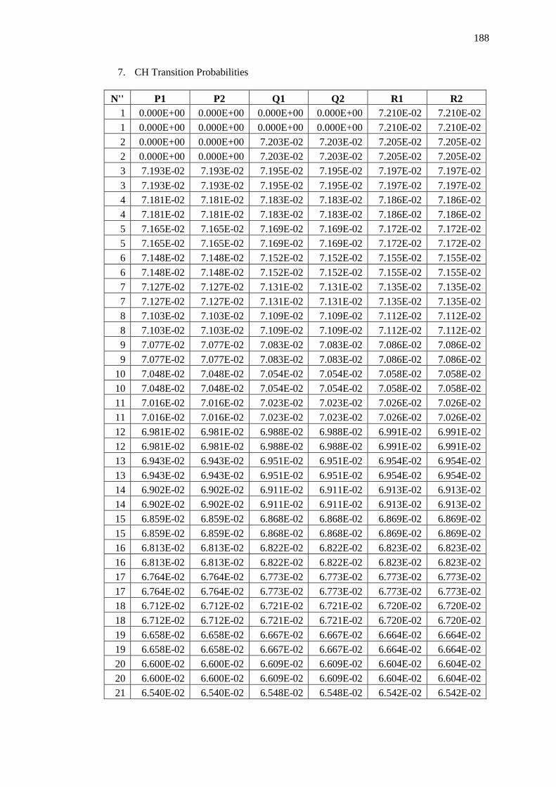
188
7. CH Transition Probabilities
N'' P1 P2 Q1 Q2 R1 R2 1 0.000E+00 0.000E+00 0.000E+00 0.000E+00 7.210E-02 7.210E-02 1 0.000E+00 0.000E+00 0.000E+00 0.000E+00 7.210E-02 7.210E-02 2 0.000E+00 0.000E+00 7.203E-02 7.203E-02 7.205E-02 7.205E-02 2 0.000E+00 0.000E+00 7.203E-02 7.203E-02 7.205E-02 7.205E-02 3 7.193E-02 7.193E-02 7.195E-02 7.195E-02 7.197E-02 7.197E-02 3 7.193E-02 7.193E-02 7.195E-02 7.195E-02 7.197E-02 7.197E-02 4 7.181E-02 7.181E-02 7.183E-02 7.183E-02 7.186E-02 7.186E-02 4 7.181E-02 7.181E-02 7.183E-02 7.183E-02 7.186E-02 7.186E-02 5 7.165E-02 7.165E-02 7.169E-02 7.169E-02 7.172E-02 7.172E-02 5 7.165E-02 7.165E-02 7.169E-02 7.169E-02 7.172E-02 7.172E-02 6 7.148E-02 7.148E-02 7.152E-02 7.152E-02 7.155E-02 7.155E-02 6 7.148E-02 7.148E-02 7.152E-02 7.152E-02 7.155E-02 7.155E-02 7 7.127E-02 7.127E-02 7.131E-02 7.131E-02 7.135E-02 7.135E-02 7 7.127E-02 7.127E-02 7.131E-02 7.131E-02 7.135E-02 7.135E-02 8 7.103E-02 7.103E-02 7.109E-02 7.109E-02 7.112E-02 7.112E-02 8 7.103E-02 7.103E-02 7.109E-02 7.109E-02 7.112E-02 7.112E-02 9 7.077E-02 7.077E-02 7.083E-02 7.083E-02 7.086E-02 7.086E-02 9 7.077E-02 7.077E-02 7.083E-02 7.083E-02 7.086E-02 7.086E-02
10 7.048E-02 7.048E-02 7.054E-02 7.054E-02 7.058E-02 7.058E-02 10 7.048E-02 7.048E-02 7.054E-02 7.054E-02 7.058E-02 7.058E-02 11 7.016E-02 7.016E-02 7.023E-02 7.023E-02 7.026E-02 7.026E-02 11 7.016E-02 7.016E-02 7.023E-02 7.023E-02 7.026E-02 7.026E-02 12 6.981E-02 6.981E-02 6.988E-02 6.988E-02 6.991E-02 6.991E-02 12 6.981E-02 6.981E-02 6.988E-02 6.988E-02 6.991E-02 6.991E-02 13 6.943E-02 6.943E-02 6.951E-02 6.951E-02 6.954E-02 6.954E-02 13 6.943E-02 6.943E-02 6.951E-02 6.951E-02 6.954E-02 6.954E-02 14 6.902E-02 6.902E-02 6.911E-02 6.911E-02 6.913E-02 6.913E-02 14 6.902E-02 6.902E-02 6.911E-02 6.911E-02 6.913E-02 6.913E-02 15 6.859E-02 6.859E-02 6.868E-02 6.868E-02 6.869E-02 6.869E-02 15 6.859E-02 6.859E-02 6.868E-02 6.868E-02 6.869E-02 6.869E-02 16 6.813E-02 6.813E-02 6.822E-02 6.822E-02 6.823E-02 6.823E-02 16 6.813E-02 6.813E-02 6.822E-02 6.822E-02 6.823E-02 6.823E-02 17 6.764E-02 6.764E-02 6.773E-02 6.773E-02 6.773E-02 6.773E-02 17 6.764E-02 6.764E-02 6.773E-02 6.773E-02 6.773E-02 6.773E-02 18 6.712E-02 6.712E-02 6.721E-02 6.721E-02 6.720E-02 6.720E-02 18 6.712E-02 6.712E-02 6.721E-02 6.721E-02 6.720E-02 6.720E-02 19 6.658E-02 6.658E-02 6.667E-02 6.667E-02 6.664E-02 6.664E-02 19 6.658E-02 6.658E-02 6.667E-02 6.667E-02 6.664E-02 6.664E-02 20 6.600E-02 6.600E-02 6.609E-02 6.609E-02 6.604E-02 6.604E-02 20 6.600E-02 6.600E-02 6.609E-02 6.609E-02 6.604E-02 6.604E-02 21 6.540E-02 6.540E-02 6.548E-02 6.548E-02 6.542E-02 6.542E-02
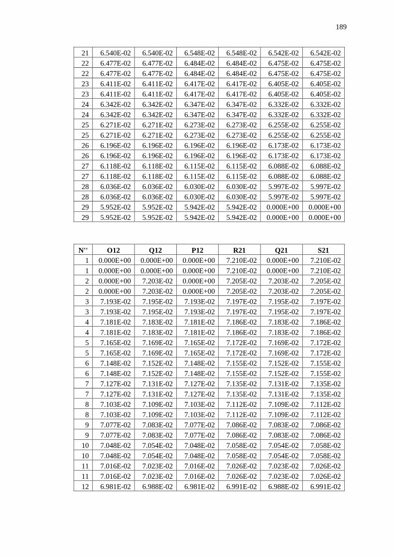
189
21 6.540E-02 6.540E-02 6.548E-02 6.548E-02 6.542E-02 6.542E-02 22 6.477E-02 6.477E-02 6.484E-02 6.484E-02 6.475E-02 6.475E-02 22 6.477E-02 6.477E-02 6.484E-02 6.484E-02 6.475E-02 6.475E-02 23 6.411E-02 6.411E-02 6.417E-02 6.417E-02 6.405E-02 6.405E-02 23 6.411E-02 6.411E-02 6.417E-02 6.417E-02 6.405E-02 6.405E-02 24 6.342E-02 6.342E-02 6.347E-02 6.347E-02 6.332E-02 6.332E-02 24 6.342E-02 6.342E-02 6.347E-02 6.347E-02 6.332E-02 6.332E-02 25 6.271E-02 6.271E-02 6.273E-02 6.273E-02 6.255E-02 6.255E-02 25 6.271E-02 6.271E-02 6.273E-02 6.273E-02 6.255E-02 6.255E-02 26 6.196E-02 6.196E-02 6.196E-02 6.196E-02 6.173E-02 6.173E-02 26 6.196E-02 6.196E-02 6.196E-02 6.196E-02 6.173E-02 6.173E-02 27 6.118E-02 6.118E-02 6.115E-02 6.115E-02 6.088E-02 6.088E-02 27 6.118E-02 6.118E-02 6.115E-02 6.115E-02 6.088E-02 6.088E-02 28 6.036E-02 6.036E-02 6.030E-02 6.030E-02 5.997E-02 5.997E-02 28 6.036E-02 6.036E-02 6.030E-02 6.030E-02 5.997E-02 5.997E-02 29 5.952E-02 5.952E-02 5.942E-02 5.942E-02 0.000E+00 0.000E+00 29 5.952E-02 5.952E-02 5.942E-02 5.942E-02 0.000E+00 0.000E+00
N'' O12 Q12 P12 R21 Q21 S21 1 0.000E+00 0.000E+00 0.000E+00 7.210E-02 0.000E+00 7.210E-02 1 0.000E+00 0.000E+00 0.000E+00 7.210E-02 0.000E+00 7.210E-02 2 0.000E+00 7.203E-02 0.000E+00 7.205E-02 7.203E-02 7.205E-02 2 0.000E+00 7.203E-02 0.000E+00 7.205E-02 7.203E-02 7.205E-02 3 7.193E-02 7.195E-02 7.193E-02 7.197E-02 7.195E-02 7.197E-02 3 7.193E-02 7.195E-02 7.193E-02 7.197E-02 7.195E-02 7.197E-02 4 7.181E-02 7.183E-02 7.181E-02 7.186E-02 7.183E-02 7.186E-02 4 7.181E-02 7.183E-02 7.181E-02 7.186E-02 7.183E-02 7.186E-02 5 7.165E-02 7.169E-02 7.165E-02 7.172E-02 7.169E-02 7.172E-02 5 7.165E-02 7.169E-02 7.165E-02 7.172E-02 7.169E-02 7.172E-02 6 7.148E-02 7.152E-02 7.148E-02 7.155E-02 7.152E-02 7.155E-02 6 7.148E-02 7.152E-02 7.148E-02 7.155E-02 7.152E-02 7.155E-02 7 7.127E-02 7.131E-02 7.127E-02 7.135E-02 7.131E-02 7.135E-02 7 7.127E-02 7.131E-02 7.127E-02 7.135E-02 7.131E-02 7.135E-02 8 7.103E-02 7.109E-02 7.103E-02 7.112E-02 7.109E-02 7.112E-02 8 7.103E-02 7.109E-02 7.103E-02 7.112E-02 7.109E-02 7.112E-02 9 7.077E-02 7.083E-02 7.077E-02 7.086E-02 7.083E-02 7.086E-02 9 7.077E-02 7.083E-02 7.077E-02 7.086E-02 7.083E-02 7.086E-02
10 7.048E-02 7.054E-02 7.048E-02 7.058E-02 7.054E-02 7.058E-02 10 7.048E-02 7.054E-02 7.048E-02 7.058E-02 7.054E-02 7.058E-02 11 7.016E-02 7.023E-02 7.016E-02 7.026E-02 7.023E-02 7.026E-02 11 7.016E-02 7.023E-02 7.016E-02 7.026E-02 7.023E-02 7.026E-02 12 6.981E-02 6.988E-02 6.981E-02 6.991E-02 6.988E-02 6.991E-02
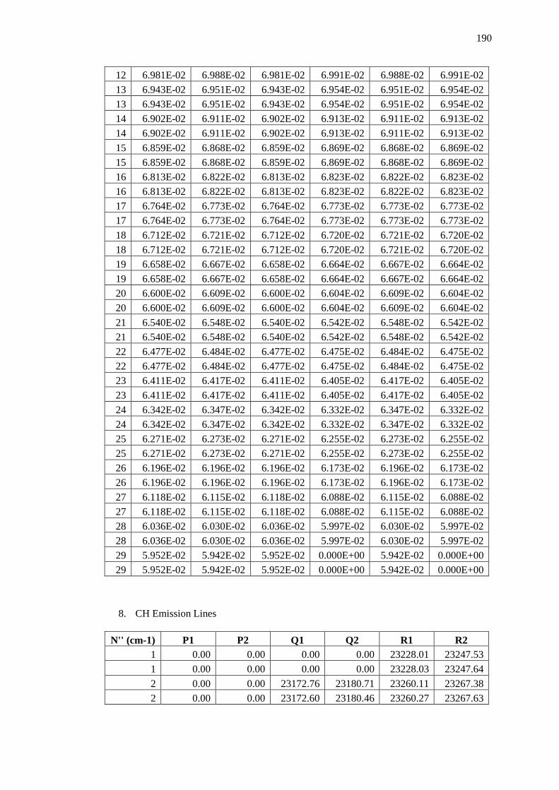
190
12 6.981E-02 6.988E-02 6.981E-02 6.991E-02 6.988E-02 6.991E-02 13 6.943E-02 6.951E-02 6.943E-02 6.954E-02 6.951E-02 6.954E-02 13 6.943E-02 6.951E-02 6.943E-02 6.954E-02 6.951E-02 6.954E-02 14 6.902E-02 6.911E-02 6.902E-02 6.913E-02 6.911E-02 6.913E-02 14 6.902E-02 6.911E-02 6.902E-02 6.913E-02 6.911E-02 6.913E-02 15 6.859E-02 6.868E-02 6.859E-02 6.869E-02 6.868E-02 6.869E-02 15 6.859E-02 6.868E-02 6.859E-02 6.869E-02 6.868E-02 6.869E-02 16 6.813E-02 6.822E-02 6.813E-02 6.823E-02 6.822E-02 6.823E-02 16 6.813E-02 6.822E-02 6.813E-02 6.823E-02 6.822E-02 6.823E-02 17 6.764E-02 6.773E-02 6.764E-02 6.773E-02 6.773E-02 6.773E-02 17 6.764E-02 6.773E-02 6.764E-02 6.773E-02 6.773E-02 6.773E-02 18 6.712E-02 6.721E-02 6.712E-02 6.720E-02 6.721E-02 6.720E-02 18 6.712E-02 6.721E-02 6.712E-02 6.720E-02 6.721E-02 6.720E-02 19 6.658E-02 6.667E-02 6.658E-02 6.664E-02 6.667E-02 6.664E-02 19 6.658E-02 6.667E-02 6.658E-02 6.664E-02 6.667E-02 6.664E-02 20 6.600E-02 6.609E-02 6.600E-02 6.604E-02 6.609E-02 6.604E-02 20 6.600E-02 6.609E-02 6.600E-02 6.604E-02 6.609E-02 6.604E-02 21 6.540E-02 6.548E-02 6.540E-02 6.542E-02 6.548E-02 6.542E-02 21 6.540E-02 6.548E-02 6.540E-02 6.542E-02 6.548E-02 6.542E-02 22 6.477E-02 6.484E-02 6.477E-02 6.475E-02 6.484E-02 6.475E-02 22 6.477E-02 6.484E-02 6.477E-02 6.475E-02 6.484E-02 6.475E-02 23 6.411E-02 6.417E-02 6.411E-02 6.405E-02 6.417E-02 6.405E-02 23 6.411E-02 6.417E-02 6.411E-02 6.405E-02 6.417E-02 6.405E-02 24 6.342E-02 6.347E-02 6.342E-02 6.332E-02 6.347E-02 6.332E-02 24 6.342E-02 6.347E-02 6.342E-02 6.332E-02 6.347E-02 6.332E-02 25 6.271E-02 6.273E-02 6.271E-02 6.255E-02 6.273E-02 6.255E-02 25 6.271E-02 6.273E-02 6.271E-02 6.255E-02 6.273E-02 6.255E-02 26 6.196E-02 6.196E-02 6.196E-02 6.173E-02 6.196E-02 6.173E-02 26 6.196E-02 6.196E-02 6.196E-02 6.173E-02 6.196E-02 6.173E-02 27 6.118E-02 6.115E-02 6.118E-02 6.088E-02 6.115E-02 6.088E-02 27 6.118E-02 6.115E-02 6.118E-02 6.088E-02 6.115E-02 6.088E-02 28 6.036E-02 6.030E-02 6.036E-02 5.997E-02 6.030E-02 5.997E-02 28 6.036E-02 6.030E-02 6.036E-02 5.997E-02 6.030E-02 5.997E-02 29 5.952E-02 5.942E-02 5.952E-02 0.000E+00 5.942E-02 0.000E+00 29 5.952E-02 5.942E-02 5.952E-02 0.000E+00 5.942E-02 0.000E+00
8. CH Emission Lines
N'' (cm-1) P1 P2 Q1 Q2 R1 R2 1 0.00 0.00 0.00 0.00 23228.01 23247.53 1 0.00 0.00 0.00 0.00 23228.03 23247.64 2 0.00 0.00 23172.76 23180.71 23260.11 23267.38 2 0.00 0.00 23172.60 23180.46 23260.27 23267.63

191
3 23088.14 23093.96 23176.03 23181.38 23292.01 23296.91 3 23088.52 23094.45 23175.65 23180.88 23292.39 23297.40 4 23062.72 23066.91 23179.75 23183.75 23324.19 23327.81 4 23063.39 23067.72 23179.08 23182.94 23324.86 23328.63 5 23037.96 23041.16 23184.10 23187.25 23356.74 23359.54 5 23039.00 23042.37 23183.07 23186.04 23357.77 23360.75 6 23013.98 23016.50 23189.13 23191.68 23389.68 23391.90 6 23015.45 23018.17 23187.66 23190.00 23391.15 23393.57 7 22990.85 22992.85 23194.85 23196.95 23423.00 23424.76 7 22992.82 22995.06 23192.87 23194.74 23424.98 23426.97 8 22968.59 22970.20 23201.27 23203.02 23456.65 23458.05 8 22971.14 22973.00 23198.72 23200.21 23459.20 23460.86 9 22947.25 22948.52 23208.38 23209.83 23490.59 23491.69 9 22950.45 22952.00 23205.18 23206.36 23493.79 23495.16
10 22926.83 22972.84 23216.15 23217.36 23524.77 23525.61 10 22930.74 22932.03 23212.24 23213.16 23528.67 23529.81 11 22907.37 22908.13 23224.56 23225.56 23559.13 23559.75 11 22912.04 22913.11 23219.89 23220.58 23563.80 23564.73 12 22888.86 22889.41 23233.59 23234.39 23593.61 23594.04 12 22894.35 22895.22 23228.09 23228.58 23599.11 23599.85 13 22871.30 22871.68 23243.19 23243.82 23628.15 23628.41 13 22877.67 22878.37 23236.82 23237.13 23634.52 23635.10 14 22854.70 22854.91 23253.32 23253.81 23662.68 23662.79 14 22861.99 22862.53 23246.03 23246.19 23669.98 23670.41 15 22839.04 22839.11 23263.95 23264.29 23697.13 23697.10 15 22847.30 22847.70 23255.69 23255.71 23705.40 23705.69 16 22824.31 22824.25 23275.03 23275.24 23731.42 23731.27 16 22833.59 22833.85 23265.76 23265.64 23740.71 23740.86 17 22810.51 22810.33 23286.50 23286.58 23765.49 23765.22 17 22820.84 22820.96 23276.18 23275.95 23775.81 23775.85 18 22797.59 22797.31 23298.31 23298.27 23799.23 23798.87 18 22809.00 22809.00 23286.91 23286.57 23810.64 23810.56 19 22785.54 22785.16 23310.39 23310.23 23832.58 23832.12 19 22798.06 22797.94 23297.88 23297.46 23845.11 23844.90 20 22774.32 22773.86 23322.68 23322.41 23865.45 23864.91 20 22787.98 22787.74 23309.04 23308.53 23879.10 23878.79 21 22763.89 22763.36 23335.11 23334.73 23897.73 23897.13 21 22778.71 22778.36 23320.32 23319.74 23912.54 23912.13 22 22754.21 22753.61 23347.61 23347.12 23929.35 23928.68 22 22770.19 22769.74 23331.64 23331.00 23945.33 23944.81 23 22745.22 22744.56 23360.09 23359.50 23960.20 23959.48 23 22762.38 22761.82 23342.95 23342.25 23977.36 23976.74 24 22736.87 22736.16 23372.47 23371.78 23990.18 23989.42
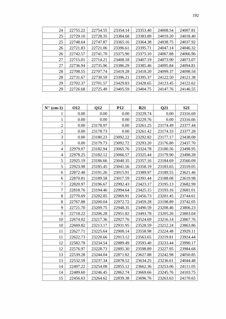
192
24 22755.22 22754.55 23354.14 23353.40 24008.54 24007.81 25 22729.10 22728.35 23384.68 23383.89 24019.20 24018.40 25 22748.64 22747.87 23365.16 23364.38 24038.75 24037.92 26 22721.83 22721.06 23396.61 23395.71 24047.14 24046.32 26 22742.57 22741.70 23375.90 23375.10 24067.88 24066.96 27 22715.01 22714.21 23408.18 23407.19 24073.90 24073.07 27 22736.94 22735.96 23386.29 23385.46 24095.84 24094.81 28 22708.55 22707.74 23419.28 23418.20 24099.37 24098.54 28 22731.67 22730.59 23396.21 23395.37 24122.50 24121.38 29 22702.37 22701.57 23429.83 23428.65 24123.45 24122.62 29 22726.68 22725.49 23405.59 23404.75 24147.76 24146.55
N'' (cm-1) O12 Q12 P12 R21 Q21 S21 1 0.00 0.00 0.00 23229.74 0.00 23316.69 1 0.00 0.00 0.00 23229.76 0.00 23316.66 2 0.00 23178.97 0.00 23261.25 23174.49 23377.44 2 0.00 23178.73 0.00 23261.42 23174.33 23377.28 3 0.00 23180.23 23092.22 23292.82 23177.17 23438.08 3 0.00 23179.73 23092.72 23293.20 23176.80 23437.70 4 22979.07 23182.94 23065.76 23324.78 23180.56 23498.95 4 22978.25 23182.12 23066.57 23325.44 23179.90 23498.28 5 22925.19 23186.66 23040.35 23357.16 23184.69 23560.09 5 22923.98 23185.45 23041.56 23358.19 23183.65 23559.05 6 22872.48 23191.26 23015.91 23389.97 23189.55 23621.46 6 22870.81 23189.58 23017.59 23391.44 23188.08 23619.98 7 22820.97 23196.67 22992.43 23423.17 23195.13 23682.99 7 22818.76 23194.46 22994.64 23425.15 23193.16 23681.01 8 22770.69 23202.85 22969.91 23456.73 23201.45 23744.61 8 22767.88 23200.04 22972.72 23459.28 23198.89 23742.05 9 22721.70 23209.75 22948.35 23490.59 23208.46 23806.23 9 22718.22 23206.28 22951.82 23493.78 23205.26 23803.04
10 22674.02 23217.36 22927.76 23524.69 23216.14 23867.76 10 22669.82 23213.17 22931.95 23528.59 23212.24 23863.86 11 22627.71 23225.64 22908.14 23558.98 23224.48 23929.11 11 22622.73 23220.66 22913.12 23563.65 23219.81 23924.44 12 22582.78 23234.54 22889.49 23593.40 23233.44 23990.17 12 22576.97 23228.73 22895.30 23598.89 23227.95 23984.68 13 22539.28 23244.04 22871.82 23627.88 23242.98 24050.85 13 22532.59 23237.34 22878.52 23634.25 23236.61 24044.48 14 22497.22 23254.08 22855.12 23662.36 23253.06 24111.05 14 22489.60 23246.45 22862.74 23669.66 23245.76 24103.75 15 22456.63 23264.62 22839.38 23696.76 23263.63 24170.65

193
15 22448.04 23256.03 22847.96 23705.03 23255.37 24162.38 16 22417.52 23275.61 22824.57 23731.01 23274.66 24229.55 16 22407.92 23266.01 22834.17 23740.29 23265.38 24220.27 17 22379.89 23287.00 22810.70 23765.03 23286.09 24287.64 17 22369.26 23276.37 22821.33 23775.35 23275.76 24277.32 18 22343.75 23298.73 22797.73 23798.73 23297.85 24344.81 18 22332.06 23287.04 22809.42 23810.14 23286.44 24333.40 19 22309.10 23310.74 22785.63 23832.04 23309.89 24400.94 19 22296.32 23297.96 22798.41 23844.56 23297.38 24388.43 20 22275.91 23322.96 22774.36 23864.88 23322.14 24455.91 20 22262.04 23309.07 22788.25 23878.52 23308.49 24442.27 21 22244.19 23335.32 22763.89 23897.13 23334.54 24509.61 21 22229.19 23320.31 22778.90 23911.93 23319.74 24494.81 22 22213.90 23347.74 22754.18 23928.71 23347.00 24561.92 22 22197.78 23331.60 22770.31 23944.68 23331.03 24545.95 23 22185.00 23360.15 22745.17 23959.54 23359.45 24612.71 23 22167.75 23342.88 22762.43 23976.69 23342.30 24595.56 24 22157.47 23372.46 22736.80 23989.50 23371.81 24661.86 24 22319.10 23354.06 22755.20 24007.83 23353.47 24643.53 25 22131.26 23384.59 22729.02 24018.49 23383.99 24709.25 25 22111.77 23365.06 22748.54 24038.01 23364.46 24689.73 26 22106.33 23396.45 22721.75 24046.42 23395.89 24754.75 26 22085.71 23375.80 22742.39 24067.13 23375.18 24734.04 27 22082.61 23407.94 22714.93 24073.16 23407.45 24798.24 27 22060.89 23386.18 22736.68 24095.07 23385.54 24776.34 28 22060.05 23418.97 22708.47 24098.62 23418.54 24839.59 28 22037.24 23396.11 22731.33 24121.71 23395.45 24816.51 29 22038.59 23429.44 22702.31 24122.70 23429.07 24878.69 29 22014.70 23405.50 22726.25 24146.96 23404.81 24854.44
9. CH Spontaneous Emission Coefficients
N'' (s-1) P1 P2 Q1 Q2 R1 R2
1 0.000E+00 0.000E+00 0.000E+00 0.000E+00 9.263E+05 9.286E+05 1 0.000E+00 0.000E+00 0.000E+00 0.000E+00 9.263E+05 9.286E+05 2 0.000E+00 0.000E+00 5.289E+05 3.945E+05 8.032E+05 7.612E+05 2 0.000E+00 0.000E+00 5.289E+05 3.945E+05 8.033E+05 7.612E+05 3 1.114E+05 9.224E+04 7.033E+05 6.360E+05 7.303E+05 7.205E+05 3 1.114E+05 9.225E+04 7.033E+05 6.359E+05 7.304E+05 7.205E+05 4 1.839E+05 1.693E+05 7.807E+05 7.478E+05 6.833E+05 6.811E+05 4 1.840E+05 1.693E+05 7.806E+05 7.477E+05 6.834E+05 6.812E+05 5 2.313E+05 2.215E+05 8.210E+05 8.027E+05 6.508E+05 6.509E+05
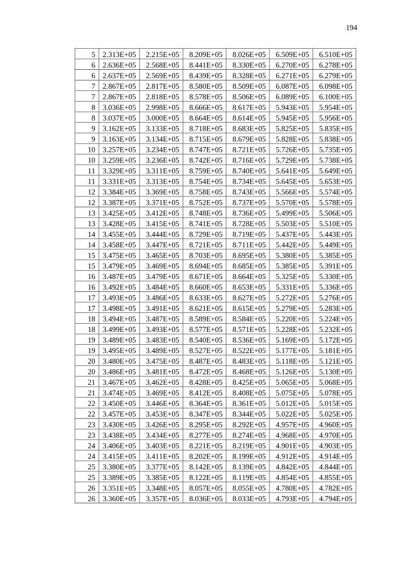
194
5 2.313E+05 2.215E+05 8.209E+05 8.026E+05 6.509E+05 6.510E+05 6 2.636E+05 2.568E+05 8.441E+05 8.330E+05 6.270E+05 6.278E+05 6 2.637E+05 2.569E+05 8.439E+05 8.328E+05 6.271E+05 6.279E+05 7 2.867E+05 2.817E+05 8.580E+05 8.509E+05 6.087E+05 6.098E+05 7 2.867E+05 2.818E+05 8.578E+05 8.506E+05 6.089E+05 6.100E+05 8 3.036E+05 2.998E+05 8.666E+05 8.617E+05 5.943E+05 5.954E+05 8 3.037E+05 3.000E+05 8.664E+05 8.614E+05 5.945E+05 5.956E+05 9 3.162E+05 3.133E+05 8.718E+05 8.683E+05 5.825E+05 5.835E+05 9 3.163E+05 3.134E+05 8.715E+05 8.679E+05 5.828E+05 5.838E+05
10 3.257E+05 3.234E+05 8.747E+05 8.721E+05 5.726E+05 5.735E+05 10 3.259E+05 3.236E+05 8.742E+05 8.716E+05 5.729E+05 5.738E+05 11 3.329E+05 3.311E+05 8.759E+05 8.740E+05 5.641E+05 5.649E+05 11 3.331E+05 3.313E+05 8.754E+05 8.734E+05 5.645E+05 5.653E+05 12 3.384E+05 3.369E+05 8.758E+05 8.743E+05 5.566E+05 5.574E+05 12 3.387E+05 3.371E+05 8.752E+05 8.737E+05 5.570E+05 5.578E+05 13 3.425E+05 3.412E+05 8.748E+05 8.736E+05 5.499E+05 5.506E+05 13 3.428E+05 3.415E+05 8.741E+05 8.728E+05 5.503E+05 5.510E+05 14 3.455E+05 3.444E+05 8.729E+05 8.719E+05 5.437E+05 5.443E+05 14 3.458E+05 3.447E+05 8.721E+05 8.711E+05 5.442E+05 5.449E+05 15 3.475E+05 3.465E+05 8.703E+05 8.695E+05 5.380E+05 5.385E+05 15 3.479E+05 3.469E+05 8.694E+05 8.685E+05 5.385E+05 5.391E+05 16 3.487E+05 3.479E+05 8.671E+05 8.664E+05 5.325E+05 5.330E+05 16 3.492E+05 3.484E+05 8.660E+05 8.653E+05 5.331E+05 5.336E+05 17 3.493E+05 3.486E+05 8.633E+05 8.627E+05 5.272E+05 5.276E+05 17 3.498E+05 3.491E+05 8.621E+05 8.615E+05 5.279E+05 5.283E+05 18 3.494E+05 3.487E+05 8.589E+05 8.584E+05 5.220E+05 5.224E+05 18 3.499E+05 3.493E+05 8.577E+05 8.571E+05 5.228E+05 5.232E+05 19 3.489E+05 3.483E+05 8.540E+05 8.536E+05 5.169E+05 5.172E+05 19 3.495E+05 3.489E+05 8.527E+05 8.522E+05 5.177E+05 5.181E+05 20 3.480E+05 3.475E+05 8.487E+05 8.483E+05 5.118E+05 5.121E+05 20 3.486E+05 3.481E+05 8.472E+05 8.468E+05 5.126E+05 5.130E+05 21 3.467E+05 3.462E+05 8.428E+05 8.425E+05 5.065E+05 5.068E+05 21 3.474E+05 3.469E+05 8.412E+05 8.408E+05 5.075E+05 5.078E+05 22 3.450E+05 3.446E+05 8.364E+05 8.361E+05 5.012E+05 5.015E+05 22 3.457E+05 3.453E+05 8.347E+05 8.344E+05 5.022E+05 5.025E+05 23 3.430E+05 3.426E+05 8.295E+05 8.292E+05 4.957E+05 4.960E+05 23 3.438E+05 3.434E+05 8.277E+05 8.274E+05 4.968E+05 4.970E+05 24 3.406E+05 3.403E+05 8.221E+05 8.219E+05 4.901E+05 4.903E+05 24 3.415E+05 3.411E+05 8.202E+05 8.199E+05 4.912E+05 4.914E+05 25 3.380E+05 3.377E+05 8.142E+05 8.139E+05 4.842E+05 4.844E+05 25 3.389E+05 3.385E+05 8.122E+05 8.119E+05 4.854E+05 4.855E+05 26 3.351E+05 3.348E+05 8.057E+05 8.055E+05 4.780E+05 4.782E+05 26 3.360E+05 3.357E+05 8.036E+05 8.033E+05 4.793E+05 4.794E+05

195
27 3.318E+05 3.316E+05 7.966E+05 7.964E+05 4.716E+05 4.717E+05 27 3.328E+05 3.325E+05 7.944E+05 7.942E+05 4.728E+05 4.730E+05 28 3.283E+05 3.281E+05 7.870E+05 7.867E+05 4.647E+05 4.649E+05 28 3.293E+05 3.291E+05 7.846E+05 7.844E+05 4.661E+05 4.662E+05 29 3.246E+05 3.243E+05 7.766E+05 7.764E+05 0.000E+00 0.000E+00 29 3.256E+05 3.254E+05 7.742E+05 7.740E+05 0.000E+00 0.000E+00
N'' (s-1) O12 Q12 P12 R21 Q21 S21
1 0.000E+00 0.000E+00 0.000E+00 3.412E+05 0.000E+00 5.877E+04 1 0.000E+00 0.000E+00 0.000E+00 3.412E+05 0.000E+00 5.877E+04 2 0.000E+00 2.225E+05 0.000E+00 1.516E+05 8.230E+04 2.339E+04 2 0.000E+00 2.225E+05 0.000E+00 1.516E+05 8.230E+04 2.339E+04 3 0.000E+00 1.062E+05 4.313E+04 8.081E+04 6.116E+04 1.230E+04 3 0.000E+00 1.062E+05 4.313E+04 8.081E+04 6.116E+04 1.229E+04 4 2.092E+03 6.183E+04 3.448E+04 4.980E+04 4.120E+04 7.510E+03 4 2.092E+03 6.182E+04 3.449E+04 4.980E+04 4.119E+04 7.509E+03 5 2.159E+03 4.033E+04 2.560E+04 3.363E+04 2.919E+04 5.041E+03 5 2.159E+03 4.033E+04 2.561E+04 3.364E+04 2.918E+04 5.040E+03 6 1.856E+03 2.832E+04 1.928E+04 2.419E+04 2.163E+04 3.609E+03 6 1.856E+03 2.832E+04 1.928E+04 2.420E+04 2.163E+04 3.609E+03 7 1.537E+03 2.095E+04 1.489E+04 1.821E+04 1.662E+04 2.709E+03 7 1.536E+03 2.094E+04 1.489E+04 1.822E+04 1.662E+04 2.708E+03 8 1.267E+03 1.610E+04 1.178E+04 1.420E+04 1.315E+04 2.106E+03 8 1.267E+03 1.610E+04 1.178E+04 1.420E+04 1.314E+04 2.105E+03 9 1.052E+03 1.275E+04 9.512E+03 1.137E+04 1.064E+04 1.684E+03 9 1.052E+03 1.274E+04 9.516E+03 1.137E+04 1.064E+04 1.683E+03
10 8.817E+02 1.033E+04 7.823E+03 9.301E+03 8.777E+03 1.376E+03 10 8.812E+02 1.033E+04 7.827E+03 9.306E+03 8.773E+03 1.376E+03 11 7.416E+02 8.533E+03 6.532E+03 7.747E+03 7.356E+03 1.146E+03 11 7.456E+02 8.528E+03 6.536E+03 7.752E+03 7.352E+03 1.145E+03 12 6.373E+02 7.160E+03 5.526E+03 6.548E+03 6.247E+03 9.684E+02 12 6.368E+02 7.154E+03 5.530E+03 6.552E+03 6.243E+03 9.677E+02 13 5.490E+02 6.087E+03 4.727E+03 5.603E+03 5.366E+03 8.288E+02 13 5.485E+02 6.082E+03 4.732E+03 5.608E+03 5.362E+03 8.282E+02 14 4.767E+02 5.233E+03 4.084E+03 4.846E+03 4.654E+03 7.171E+02 14 4.762E+02 5.228E+03 4.088E+03 4.850E+03 4.650E+03 7.164E+02 15 4.169E+02 4.543E+03 3.558E+03 4.229E+03 4.071E+03 6.262E+02 15 4.164E+02 4.538E+03 3.562E+03 4.234E+03 4.067E+03 6.256E+02 16 3.669E+02 3.976E+03 3.122E+03 3.720E+03 3.587E+03 5.512E+02 16 3.664E+02 3.971E+03 3.126E+03 3.724E+03 3.583E+03 5.506E+02 17 3.248E+02 3.505E+03 2.758E+03 3.295E+03 3.182E+03 4.886E+02

196
17 3.243E+02 3.501E+03 2.762E+03 3.299E+03 3.177E+03 4.880E+02 18 2.890E+02 3.110E+03 2.451E+03 2.936E+03 2.838E+03 4.358E+02 18 2.885E+02 3.105E+03 2.455E+03 2.940E+03 2.834E+03 4.352E+02 19 2.584E+02 2.775E+03 2.189E+03 2.630E+03 2.544E+03 3.908E+02 19 2.579E+02 2.770E+03 2.193E+03 2.634E+03 2.540E+03 3.902E+02 20 2.319E+02 2.488E+03 1.965E+03 2.366E+03 2.291E+03 3.520E+02 20 2.315E+02 2.484E+03 1.968E+03 2.370E+03 2.287E+03 3.514E+02 21 2.090E+02 2.241E+03 1.770E+03 2.138E+03 2.071E+03 3.185E+02 21 2.086E+02 2.237E+03 1.774E+03 2.142E+03 2.067E+03 3.179E+02 22 1.891E+02 2.026E+03 1.601E+03 1.939E+03 1.880E+03 2.892E+02 22 1.886E+02 2.022E+03 1.605E+03 1.943E+03 1.876E+03 2.886E+02 23 1.715E+02 1.839E+03 1.453E+03 1.765E+03 1.711E+03 2.634E+02 23 1.711E+02 1.835E+03 1.456E+03 1.768E+03 1.707E+03 2.628E+02 24 1.561E+02 1.673E+03 1.323E+03 1.610E+03 1.562E+03 2.406E+02 24 1.557E+02 1.670E+03 1.326E+03 1.614E+03 1.558E+03 2.401E+02 25 1.424E+02 1.527E+03 1.207E+03 1.473E+03 1.429E+03 2.203E+02 25 1.420E+02 1.524E+03 1.210E+03 1.477E+03 1.426E+03 2.198E+02 26 1.302E+02 1.397E+03 1.104E+03 1.350E+03 1.311E+03 2.022E+02 26 1.298E+02 1.394E+03 1.107E+03 1.354E+03 1.308E+03 2.017E+02 27 1.193E+02 1.281E+03 1.013E+03 1.240E+03 1.205E+03 1.859E+02 27 1.189E+02 1.278E+03 1.016E+03 1.243E+03 1.201E+03 1.854E+02 28 1.095E+02 1.177E+03 9.303E+02 1.141E+03 1.109E+03 1.711E+02 28 1.092E+02 1.173E+03 9.331E+02 1.144E+03 1.106E+03 1.707E+02 29 1.007E+02 1.083E+03 8.560E+02 0.000E+00 1.022E+03 0.000E+00 29 1.004E+02 1.079E+03 8.588E+02 0.000E+00 1.019E+03 0.000E+00 10. CH Honl London Factors
N'' P1 P2 Q1 Q2 R1 R2 1 0.000 0.000 0.000 0.000 3.015 2.010 1 0.000 0.000 0.000 0.000 3.015 2.010 2 0.000 0.000 1.736 0.862 3.474 2.467 2 0.000 0.000 1.736 0.862 3.474 2.467 3 0.370 0.204 3.079 2.087 3.936 3.105 3 0.370 0.204 3.079 2.087 3.936 3.105 4 0.819 0.565 4.277 3.276 4.408 3.660 4 0.819 0.565 4.277 3.276 4.408 3.660 5 1.294 0.991 5.406 4.403 4.887 4.188 5 1.294 0.991 5.406 4.403 4.887 4.188 6 1.780 1.444 6.495 5.493 5.371 4.704 6 1.780 1.444 6.495 5.493 5.371 4.704 7 2.271 1.913 7.562 6.559 5.858 5.215 7 2.271 1.913 7.562 6.559 5.858 5.215 8 2.766 2.390 8.613 7.611 6.347 5.722 8 2.766 2.390 8.613 7.611 6.347 5.722
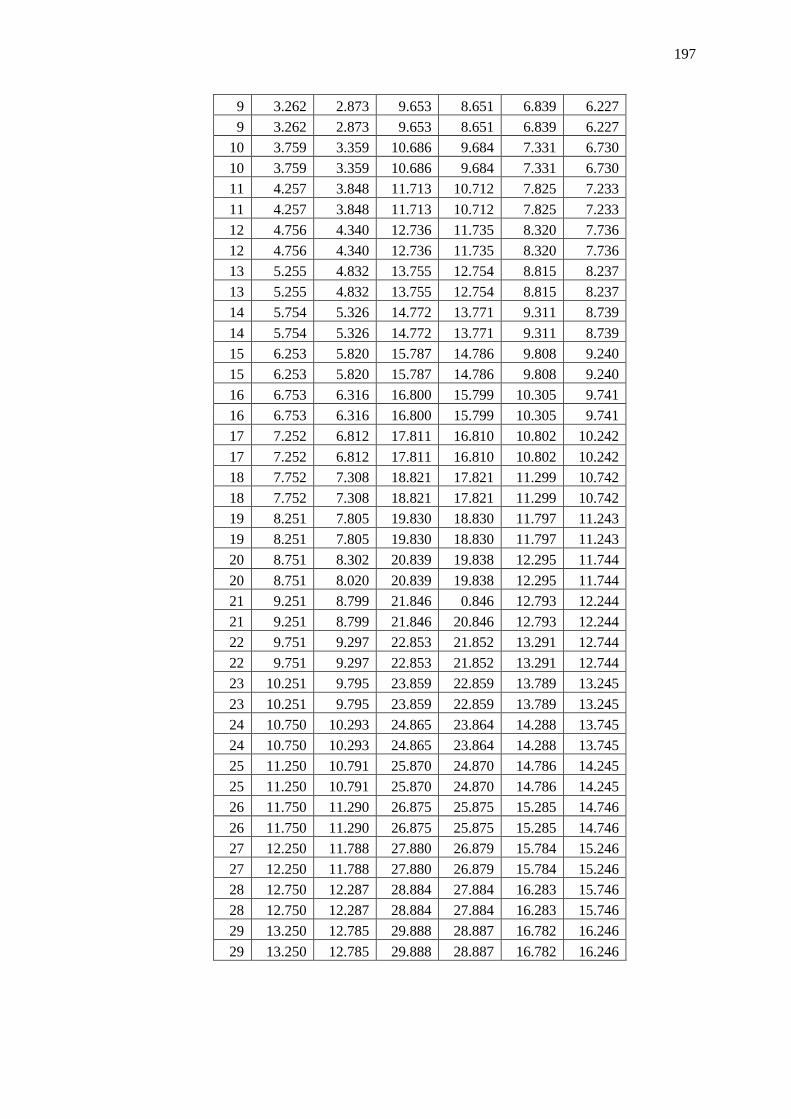
197
9 3.262 2.873 9.653 8.651 6.839 6.227 9 3.262 2.873 9.653 8.651 6.839 6.227
10 3.759 3.359 10.686 9.684 7.331 6.730 10 3.759 3.359 10.686 9.684 7.331 6.730 11 4.257 3.848 11.713 10.712 7.825 7.233 11 4.257 3.848 11.713 10.712 7.825 7.233 12 4.756 4.340 12.736 11.735 8.320 7.736 12 4.756 4.340 12.736 11.735 8.320 7.736 13 5.255 4.832 13.755 12.754 8.815 8.237 13 5.255 4.832 13.755 12.754 8.815 8.237 14 5.754 5.326 14.772 13.771 9.311 8.739 14 5.754 5.326 14.772 13.771 9.311 8.739 15 6.253 5.820 15.787 14.786 9.808 9.240 15 6.253 5.820 15.787 14.786 9.808 9.240 16 6.753 6.316 16.800 15.799 10.305 9.741 16 6.753 6.316 16.800 15.799 10.305 9.741 17 7.252 6.812 17.811 16.810 10.802 10.242 17 7.252 6.812 17.811 16.810 10.802 10.242 18 7.752 7.308 18.821 17.821 11.299 10.742 18 7.752 7.308 18.821 17.821 11.299 10.742 19 8.251 7.805 19.830 18.830 11.797 11.243 19 8.251 7.805 19.830 18.830 11.797 11.243 20 8.751 8.302 20.839 19.838 12.295 11.744 20 8.751 8.020 20.839 19.838 12.295 11.744 21 9.251 8.799 21.846 0.846 12.793 12.244 21 9.251 8.799 21.846 20.846 12.793 12.244 22 9.751 9.297 22.853 21.852 13.291 12.744 22 9.751 9.297 22.853 21.852 13.291 12.744 23 10.251 9.795 23.859 22.859 13.789 13.245 23 10.251 9.795 23.859 22.859 13.789 13.245 24 10.750 10.293 24.865 23.864 14.288 13.745 24 10.750 10.293 24.865 23.864 14.288 13.745 25 11.250 10.791 25.870 24.870 14.786 14.245 25 11.250 10.791 25.870 24.870 14.786 14.245 26 11.750 11.290 26.875 25.875 15.285 14.746 26 11.750 11.290 26.875 25.875 15.285 14.746 27 12.250 11.788 27.880 26.879 15.784 15.246 27 12.250 11.788 27.880 26.879 15.784 15.246 28 12.750 12.287 28.884 27.884 16.283 15.746 28 12.750 12.287 28.884 27.884 16.283 15.746 29 13.250 12.785 29.888 28.887 16.782 16.246 29 13.250 12.785 29.888 28.887 16.782 16.246

198
N'' O12 Q12 P12 R21 Q21 S21 1 0.000 0.000 0.000 0.740 0.000 0.189 1 0.000 0.000 0.000 0.740 0.000 0.189 2 0.000 0.729 0.000 0.492 0.180 0.100 2 0.000 0.729 0.000 0.492 0.180 0.100 3 0.000 0.465 0.143 0.348 0.201 0.065 3 0.000 0.465 0.143 0.348 0.201 0.065 4 0.007 0.339 0.153 0.268 0.181 0.047 4 0.007 0.339 0.153 0.268 0.181 0.047 5 0.010 0.265 0.143 0.216 0.160 0.037 5 0.010 0.265 0.143 0.216 0.160 0.037 6 0.011 0.218 0.130 0.181 0.143 0.030 6 0.011 0.218 0.130 0.181 0.143 0.030 7 0.011 0.185 0.118 0.156 0.128 0.025 7 0.011 0.185 0.118 0.156 0.128 0.025 8 0.010 0.160 0.107 0.136 0.116 0.022 8 0.010 0.160 0.107 0.136 0.116 0.022 9 0.010 0.141 0.098 0.121 0.106 0.019 9 0.010 0.141 0.098 0.121 0.106 0.019
10 0.009 0.126 0.090 0.109 0.097 0.017 10 0.009 0.126 0.090 0.109 0.097 0.017 11 0.009 0.114 0.084 0.099 0.090 0.015 11 0.009 0.114 0.084 0.099 0.090 0.015 12 0.009 0.104 0.078 0.091 0.084 0.014 12 0.009 0.104 0.078 0.091 0.084 0.014 13 0.008 0.096 0.073 0.084 0.078 0.013 13 0.008 0.096 0.073 0.084 0.078 0.013 14 0.008 0.089 0.068 0.078 0.074 0.012 14 0.008 0.089 0.068 0.078 0.074 0.012 15 0.007 0.082 0.064 0.073 0.069 0.011 15 0.007 0.082 0.064 0.073 0.069 0.011 16 0.007 0.077 0.060 0.068 0.065 0.010 16 0.007 0.077 0.060 0.068 0.065 0.010 17 0.007 0.072 0.057 0.064 0.062 0.009 17 0.007 0.072 0.057 0.064 0.062 0.009 18 0.006 0.068 0.054 0.060 0.059 0.009 18 0.006 0.068 0.054 0.060 0.059 0.009 19 0.006 0.064 0.052 0.057 0.056 0.008 19 0.006 0.064 0.052 0.057 0.056 0.008 20 0.006 0.061 0.049 0.054 0.054 0.008 20 0.006 0.061 0.049 0.054 0.054 0.008 21 0.006 0.058 0.047 0.052 0.051 0.007 21 0.006 0.058 0.047 0.052 0.051 0.007
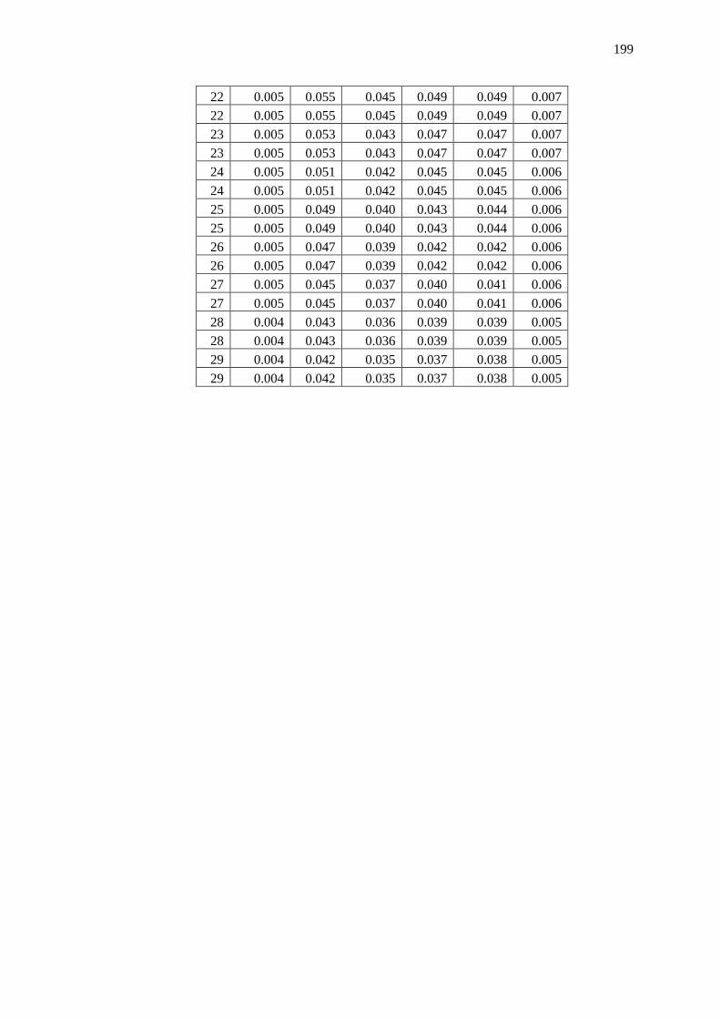
199
22 0.005 0.055 0.045 0.049 0.049 0.007 22 0.005 0.055 0.045 0.049 0.049 0.007 23 0.005 0.053 0.043 0.047 0.047 0.007 23 0.005 0.053 0.043 0.047 0.047 0.007 24 0.005 0.051 0.042 0.045 0.045 0.006 24 0.005 0.051 0.042 0.045 0.045 0.006 25 0.005 0.049 0.040 0.043 0.044 0.006 25 0.005 0.049 0.040 0.043 0.044 0.006 26 0.005 0.047 0.039 0.042 0.042 0.006 26 0.005 0.047 0.039 0.042 0.042 0.006 27 0.005 0.045 0.037 0.040 0.041 0.006 27 0.005 0.045 0.037 0.040 0.041 0.006 28 0.004 0.043 0.036 0.039 0.039 0.005 28 0.004 0.043 0.036 0.039 0.039 0.005 29 0.004 0.042 0.035 0.037 0.038 0.005 29 0.004 0.042 0.035 0.037 0.038 0.005

200
Appendix C – Subroutines and Logical Map
Logical Map:
Map of functions:
1. Optic_Correction1D.m
2. SolAngCorr.m
3. diaspectrum.m
4. absorption.m
5. Volint.m
6. partitionf.m
7. voigt.m
8. Acceptance_Angle.m
9. complexErrorFunction.m
Optic_Correction1D.m
SolAngCorr.m
Volint.m
Acceptance_Angle.m
diaspectrum.m
partitionf.m
absorption.m
partitionf.m voigt.m
complexErrorFunction.m

201
1. Optic_Correction1D.m
clc; clear all; close all; %%%%%%%%%%%%%%%%%%%%%%%%%%%%%%%%%%%%%%%%%%%%%%%%%%%%%%%%%%%%%%%%%%%%%%%%%%% %%%%%%%%%%%%%%%%%%%%%%%%%%%%%%%%%%%%%%%%%%%%%%%%%%%%%%%%%%%%%%%%%%%%%%%%%%% % Optical Diagnostic Correction Routine %%%%%%%%%%%%%%%%%%%%%%%%%%%%%%%%%%%%%%%%%%%%%%%%%%%%%%%%%%%%%%%%%%%%%%%%%%% %%%%%%%%%%%%%%%%%%%%%%%%%%%%%%%%%%%%%%%%%%%%%%%%%%%%%%%%%%%%%%%%%%%%%%%%%%% %Authors: Tristan Fuller, Michael Bedard %Version 1.2 %Updated: 3/25/2015 %This logical routine corrects CFD data for optical output. The corrections %made are for optical geometry and absorption of CH and OH related %wavelengths. The axes are in Cartesian form where the axes represent the %following: X - Displacement along axis of the combustor; Y - Distance %along width (Horizontal) of combustor; Z - Distance along width (vertical) %of combustor. 1D approximation. load('radicalsdata.mat'); tic conn = load('C:\Users\Tristan\Documents\Research and Thesis\Data\MatlabDataTristan\y.mat'); xt = round(1e10*conn.x)./1e10; yt = round(1e10*conn.y)./1e10; cont = [conn.connectivity (1:length(conn.connectivity))']; % %%%%%%%%%%%%%%%%%%%%%%%%%%%%%%%%%%%%%%%%%%%%%%%%%%%%%%%%%%%%%%%%%%%%%%%%%% % %%%%%%%%%%%%%%%%%%%%%%%%%%%%%%%%%%%%%%%%%%%%%%%%%%%%%%%%%%%%%%%%%%%%%%%%%% % Geometric Correction for Optics % %%%%%%%%%%%%%%%%%%%%%%%%%%%%%%%%%%%%%%%%%%%%%%%%%%%%%%%%%%%%%%%%%%%%%%%%%% % %%%%%%%%%%%%%%%%%%%%%%%%%%%%%%%%%%%%%%%%%%%%%%%%%%%%%%%%%%%%%%%%%%%%%%%%%% ProbCent = 0.0238252; %Location center along chamber across where probe is located (m) ProbWidth = 0.004; %Approximate threshold volume width (rectangular prism) aroun probe volume for the purpose of reducing domain. (m)

202
SliceStep = 0.2; %Slice step size to rotate domain into 3D. (rad) [INDX,xx,zz,yy,voli,GeomCorr] = SolAngCorr(ProbCent,ProbWidth,SliceStep,xt,yt,cont); % SS = [INDX,xx,zz,yy,voli,GeomCorr]; dlmwrite('ClipDomain.xls',SS); GCtime = toc; %% Directory = 'C:\Users\Tristan\Dropbox\Research Data\'; M = dlmread('ClipDomain.xls'); INDX = M(:,1); xx = M(:,2); zz = M(:,3); yy = M(:,4); voli = M(:,5); GeomCorr = M(:,6); %%%%%%%%%%%%%%%%%%%%%%%%%%%%%%%%%%%%%%%%%%%%%%%%%%%%%%%%%%%%%%%%%%%%%%%%%%% %%%%%%%%%%%%%%%%%%%%%%%%%%%%%%%%%%%%%%%%%%%%%%%%%%%%%%%%%%%%%%%%%%%%%%%%%%% % Spectroscopic Chemiluminescent Emissions %%%%%%%%%%%%%%%%%%%%%%%%%%%%%%%%%%%%%%%%%%%%%%%%%%%%%%%%%%%%%%%%%%%%%%%%%%% %%%%%%%%%%%%%%%%%%%%%%%%%%%%%%%%%%%%%%%%%%%%%%%%%%%%%%%%%%%%%%%%%%%%%%%%%%% tic % Load CFD Data CO2 = load([Directory 'MatlabDataTristan\CO2.mat']); OH = load([Directory 'MatlabDataTristan\OH.mat']); CH = load([Directory 'MatlabDataTristan\CH.mat']); OHstar = load([Directory 'MatlabDataTristan\OHstar.mat']); CHstar = load([Directory 'MatlabDataTristan\CHstar.mat']); D = load([Directory 'MatlabDataTristan\D.mat']); Tp = load([Directory 'MatlabDataTristan\T.mat']); P = load([Directory 'MatlabDataTristan\P.mat']); % Load Emission/Abosrption Constants % OH Parameters rotcOH = xlsread([Directory 'OHRotConst.xls'],1,'B2:B6'); OHEt = xlsread([Directory 'OHRotEm.xls'],1,'A2:M41'); OHE = reshape(OHEt(1:40,2:end),12*40,1); OHN = repmat(OHEt(1:40,1),12,1); OHLt = xlsread([Directory 'OHLinePos.xls'],1,'B2:M41'); OHW = reshape(OHLt,12*40,1); % CH parameters rotcCH = xlsread([Directory 'CHRotConst.xls'],1,'B2:B6'); CHEt = xlsread([Directory 'CHRotEm.xls'],1,'A2:M59'); CHE = reshape(CHEt(1:58,2:end),12*58,1); CHN = repmat(CHEt(1:58,1),12,1); CHLt = xlsread([Directory 'CHLinePos.xls'],1,'B2:M59'); CHW = reshape(CHLt,12*58,1); MCH = 13.01864; %Error in value = 0.002175% %g/mol or amu
203
MOH = 17.0073; %Error in value = 0.006683% Mol = 6.02214127e23; %Avogadro's Number (mol^-1) h = 6.6260695729e-34; %Planck's Constant (m^2 kg s^-1) kb = 1.3806488e-23; %Boltzmann Constant c = 299792458; %Speed of light (m/s) waoCH = xlsread([Directory 'CHLinePos.xls'],1,'G2'); waoOH = xlsread([Directory 'OHLinePos.xls'],1,'B2'); % Line and Gas properties, assumption that homogenous linewidth is 0.5cm^-1 (HWHM). gamc = 0.5; rotconstCH = [rotcCH' 0 4]; rotconstOH = [rotcOH' 0 4]; % Point of Focus XFoc = [0.0238252; min(yy) - (0.00079375*(max(yy) - min(yy)))/(max(xx) - 0.00079375); 0]; %%%%%%%%%%%%%%%%%%%%%%%%%%%%%%%%%%%%%%%%%%%%%%%%%%%%%%%%%%%%%%%%%%%%%%%%%%% % Construction of Optical Path per Emission Source %%%%%%%%%%%%%%%%%%%%%%%%%%%%%%%%%%%%%%%%%%%%%%%%%%%%%%%%%%%%%%%%%%%%%%%%%%% % Shells method using equal sized shells, total time NS = 100; ttot = 151; %Initialise variables Pp = zeros(NS,1); GeomCR = zeros(NS,1); NCHstar = zeros(NS,1); NOHstar = zeros(NS,1); NCH = zeros(NS,1); NOH = zeros(NS,1); NCO2 = zeros(NS,1); R = sqrt(zz.^2 + (yy - min(yy)).^2); % Radial distance from measurement. YY = 2*max(yy); dY = YY/NS; for j = 1 : NS Yold = YY; YY = YY - dY; [psi,~] = find(R <= Yold & R > YY); GeomCR(j) = sum((GeomCorr(psi)).*voli(INDX(psi)))/sum(voli(INDX(psi))); end; fprintf('Computing resultant emissions...\n\n'); h = waitbar(0,'Initializing waitbar...'); for t = 1 : ttot perc = t/ttot*100;

204
waitbar(perc/100,h,sprintf('%d/%d timesteps complete...',t,ttot)); %% Shell method using equal slices %Initialise variables emch = zeros(NS,12*58,1); emoh = zeros(NS,12*40,1); T = zeros(NS,1); YY = 2*max(yy); for j = 1 : NS Yold = YY; YY = YY - dY; [psi,~] = find(R <= Yold & R > YY); % Emission Strength (W/m^3) - Geometric Optic Correction Included (Volume Averaged) % Number densities of emitting sources NCHstar(j) = sum((CHstar.varvalues(INDX(psi),t).*D.varvalues(INDX(psi),t)*1000/MCH*Mol).*voli(INDX(psi)))/sum(voli(INDX(psi))); NOHstar(j) = sum((OHstar.varvalues(INDX(psi),t).*D.varvalues(INDX(psi),t)*1000/MOH*Mol).*voli(INDX(psi)))/sum(voli(INDX(psi))); % Number densities of absorbing sinks NCH(j) = sum((CH.varvalues(INDX(psi),t).*D.varvalues(INDX(psi),t)*1000/MCH*Mol).*voli(INDX(psi)))/sum(voli(INDX(psi))); NOH(j) = sum((OH.varvalues(INDX(psi),t).*D.varvalues(INDX(psi),t)*1000/MOH*Mol).*voli(INDX(psi)))/sum(voli(INDX(psi))); NCO2(j) = sum((CO2.varvalues(INDX(psi),t).*D.varvalues(INDX(psi),t)*1000/MOH*Mol).*voli(INDX(psi)))/sum(voli(INDX(psi))); %Average Temperature at slice T(j) = sum((Tp.varvalues(INDX(psi),t)).*voli(INDX(psi)))/sum(voli(INDX(psi))); Pp(j,1) = sum((P.varvalues(INDX(psi),t)).*voli(INDX(psi)))/sum(voli(INDX(psi))); [emcht(j,:),emoht(j,:),~,~] = diaspectrum(T(j),NCHstar(j),NOHstar(j),CHEt,CHLt,CHN,rotcCH,OHEt,OHLt,OHN,rotcOH); emch(j,:) = emcht(j,:)*GeomCR(j)*sum(voli(INDX(psi))); emoh(j,:) = emoht(j,:)*GeomCR(j)*sum(voli(INDX(psi))); end; ResEmCH = sum(emch); ResEmOH = sum(emoh); %% Output Emission Data for Each Timestep xlswrite(['NumberDensity_' num2str(t)],[NCHstar NCH NOHstar NOH NCO2],1); xlswrite(['IrradianceUnCorrected_' num2str(t)],emch',1); xlswrite(['IrradianceUnCorrected_' num2str(t)],emoh',2); %% %%%%%%%%%%%%%%%%%%%%%%%%%%%%%%%%%%%%%%%%%%%%%%%%%%%%%%%%%%%%%%%%%%%%%%%%%%%
205
%%%%%%%%%%%%%%%%%%%%%%%%%%%%%%%%%%%%%%%%%%%%%%%%%%%%%%%%%%%%%%%%%%%%%%%%%%% % Spectroscopic Abosrption Correction for Chemiluminescent Emissions %%%%%%%%%%%%%%%%%%%%%%%%%%%%%%%%%%%%%%%%%%%%%%%%%%%%%%%%%%%%%%%%%%%%%%%%%%% %%%%%%%%%%%%%%%%%%%%%%%%%%%%%%%%%%%%%%%%%%%%%%%%%%%%%%%%%%%%%%%%%%%%%%%%%%% Kch = zeros(NS,12*58,12*58); gch = zeros(NS,12*58,12*58); Koh = zeros(NS,12*40,12*40); goh = zeros(NS,12*40,12*40); emabsch = zeros(NS,12*58); emabsoh = zeros(NS,12*40); transmCH = zeros(NS,12*58); transmOH = zeros(NS,12*40); emabsch(:,:) = emch(:,:); emabsoh(:,:) = emoh(:,:); A = xlsread(['NumberDensity_' num2str(t)]); B = xlsread(['IrradianceUnCorrected_' num2str(t)],1); C = xlsread(['IrradianceUnCorrected_' num2str(t)],2); % Number densities of absorbing sinks NCH = A(:,2); NOH = A(:,4); NCO2 = A(:,5); emch = B'; emoh = C'; for i = NS : -1 : 1 % CH Line Profile for j = 1 : (12*58) [Kch(i,:,j),gch(i,:,j)] = absorption(NCH(i),T(i),CHW(j),CHW,MCH,gamc,CHE,rotconstCH,CHN); if i < NS %CH resultant emission transmCH(i,j) = 1-sum(1-exp(-Kch(i,:,j).*gch(i,:,j)*dY/2))*sum(1-exp(-Kch(i+1,:,j).*gch(i+1,:,j)*dY/2)); if transmCH(i,j) < 0 transmCH(i,j) = 0; end; else %CH resultant emission transmCH(i,j) = 1-sum(1-exp(-Kch(i,:,j).*gch(i,:,j)*dY/2)); if transmCH(i,j) < 0 transmCH(i,j) = 0; end; end; end; % OH Line Profile for j = 1 : (12*40) [Koh(i,:,j),goh(i,:,j)] = absorption(NOH(i),T(i),OHW(j),OHW,MOH,gamc,OHE,rotconstOH,OHN); if i < NS %OH resultant emission

206
transmOH(i,j) = 1-sum(1-exp(-Koh(i,:,j).*goh(i,:,j)*dY/2))*sum(1-exp(-Koh(i+1,:,j).*goh(i+1,:,j)*dY/2)); if transmOH(i,j) < 0 transmOH(i,j) = 0; end; else %OH resultant emission transmOH(i,j) = 1-sum(1-exp(-Koh(i,:,j).*goh(i,:,j)*dY/2)); if transmOH(i,j) < 0 transmOH(i,j) = 0; end; end; end; emabsch(i,:) = emch(i,:).*prod(transmCH(i:NS,:)); emabsoh(i,:) = emoh(i,:).*prod(transmOH(i:NS,:)); end; ResAbsCH = sum(emabsch); ResAbsOH = sum(emabsoh); TRCH = prod(transmCH); TROH = prod(transmOH); %% Ouput Absorption Data for Each Timestep xlswrite(['ResEmissionCH_' num2str(t)],emabsch'); xlswrite(['ResEmissionOH_' num2str(t)],emabsoh'); xlswrite(['TransmissionCH_' num2str(t)],TRCH'); xlswrite(['TransmissionOH_' num2str(t)],TROH'); xlswrite(['TransmissionDistCH_' num2str(t)],transmCH'); xlswrite(['TransmissionDistOH_' num2str(t)],transmOH'); end; close(h) fprintf('Finalizing resultant emissions...\n\n'); OpticCRtime = toc;

207
2. SolAngCorr.m
function [INDX,xx,zz,yy,voli,GeomCorr] = SolAngCorr(cc,wd,dtheta,xt,yt,cont) %%%%%%%%%%%%%%%%%%%%%%%%%%%%%%%%%%%%%%%%%%%%%%%%%%%%%%%%%%%%%%%%%%%%%%%%%%% %Subroutine to correct optic measurements due to geometry and position of %source relative to lens and measurement. The measurments are biased due %the solid angle of the radiation emission collected by the lens. %Written by: Michael Bedard 2014 %Updated by: Tristan Fuller 7 March 2015 %%%%%%%%%%%%%%%%%%%%%%%%%%%%%%%%%%%%%%%%%%%%%%%%%%%%%%%%%%%%%%%%%%%%%%%%%%% [xcnt,ycnt,voltemp] = volint(xt,yt,cont,1e10); %% Extracting local probe volume domain (rectangle section) [insidex,~] = find(abs(xcnt(:,1) - cc) < wd); % "insidex" = node values inside domain % Preparing for Revolutions of Axisymmetrix Domain theta_rad = deg2rad(linspace(0,360-dtheta,360/dtheta)); x = xcnt(insidex); r = ycnt(insidex); volt = voltemp(insidex)/(360/dtheta); % Label new points based on original domain con = repmat(cont(insidex,end),size(theta_rad,2),1); %X(x coord. for each point in azimuthal slice) X_col = repmat(x,size(theta_rad,2),1); %Y(y coord. for each point in azimuthal slice, angle of azimuthal slice) Y(:,:) = r*cos(theta_rad); Y_col = reshape(Y,size(Y,1)*size(Y,2),1); %Reform into single column %Z(z coord. for each point in azimuthal slice, angle of azimuthal slice) Z(:,:) = r*sin(theta_rad); Z_col = reshape(Z,size(Z,1)*size(Z,2),1); %Reform into single column %Volume(Volume for each cell in azimuthal slice) V_col = repmat(volt',size(theta_rad,2),1); clear xt yt x r xcenterstemp ycenterstemp cont conn voltemp %%%%%%%%%%%%%%%%%%%%%%%%%%%%%%%%%%%%%%%%%%%%%%%%%%%%%%%%%%%%%%%%%%%%%%%%%%% % Develop Formula to Determine Cell Centers that Fall within Probe Volume %%%%%%%%%%%%%%%%%%%%%%%%%%%%%%%%%%%%%%%%%%%%%%%%%%%%%%%%%%%%%%%%%%%%%%%%%%% %Define optical axis along x=0.0238252m %Opening in chamber wall is 0.0015875m %Rescale x-axis such that zero is on optical axis X_col_zero = X_col - cc; %Rescale y-axis such that zero is on chamber wall

208
Y_col_zero = Y_col - min(Y_col); %%%%%%%%%%%%%%%%%%%%%%%%%%%%%%%%%%%%%%%%%%%%%%%%%%%%%%%%%%%%%%%%%%%%%%%%%%% % Probe Volume Characteristics Determined by Optic Hardware %%%%%%%%%%%%%%%%%%%%%%%%%%%%%%%%%%%%%%%%%%%%%%%%%%%%%%%%%%%%%%%%%%%%%%%%%%% fprintf('Initializing...\n\n') Window_Thickness = 3.175; %Thickness of Window in mm Window_Refract = 1.8; %Average Index of Refraction of Window Material Air_Refract = 1.0003; %Index of Refraction of Air Aperture1_Diam = 1.587; %Diameter of First Aperture in mm Aperture2_Diam = Aperture1_Diam; %Diameter of Second Aperture in mm Aperture2_Dist = 4.79; %Distance of Aperture 2 from Aperture 1 Aperture3_Diam = 1; %Diameter of First Aperture in mm Aperture3_Dist = Aperture2_Dist + Window_Thickness; %Distance of Aperture 3 from Aperture 1 Aperture4_Diam = 1; %Diameter of Second Aperture in mm Aperture4_Dist = Aperture3_Dist + 6.22; %Distance of Aperture 4 from Aperture 1 Lens_Diam=2.5; %Diameter of Collimating Lens in mm Lens_Focal_Length = 5; %Collimating Lens Focal Length in mm Fiber_Diam = .4; %Optical Fiber Diameter in mm Fiber_Dist = Aperture4_Dist; %Distance of Fiber from Aperture 1 Lens_Dist = Aperture4_Dist;%Fiber_Dist-Lens_Focal_Length; %Separation Distance Between Aperture 1 and Lens in mm Cham_d = 1.77*25.4; %chamber diameter inc = .0001; %ray angle increment grid_spacing = 50; %%%%%%%%%%%%%%%%%%%%%%%%%%%%%%%%%%%%%%%%%%%%%%%%%%%%%%%%%%%%%%%%%%%%%%%%%%% % Calculate Extreme Rays Based on Optic Harware %%%%%%%%%%%%%%%%%%%%%%%%%%%%%%%%%%%%%%%%%%%%%%%%%%%%%%%%%%%%%%%%%%%%%%%%%%% fprintf('Calculating Extreme Rays...\n\n') %Compute Extreme Ray Angle That Passes Through First Aperture Pair Init_X_Angle = -atan((Aperture1_Diam/2)/(Aperture2_Dist/2)); %Set initial height and angle of ray based on fiber diameter and lens %location and size y0 = Aperture1_Diam/2; A0 = Init_X_Angle; Ray_Stop = Aperture1_Diam; Ray_Stop2 = 0; i = 0; j = 0; while (abs(Ray_Stop(1)) > Aperture4_Diam/2) || ... (abs(Ray_Stop2(1)) > Fiber_Diam/2) || ... (abs(Ray_Stop3(1)) > Aperture3_Diam/2) if i > 10000 A0 = Init_X_Angle; y0 = y0 - .001; i = 0; end A0 = A0 + inc;

209
%Develop Translation Matrix from Aperture 1 to Aperture 2 M1 = [[1 Aperture2_Dist]; [0 1]]; %Develop Transition Matrix from Aperture 2 to Window M2 = [[1 0]; [0 Window_Refract/Air_Refract]]; %Develop Translation Matrix through Window M3 = [[1 Window_Thickness]; [0 1]]; %Develop Transition Matrix from Window to Aperture 3 M4 = [[1 0]; [0 Air_Refract/Window_Refract]]; %Develop Translation Matrix from Aperture 3 to Aperture 4 M5 = [[1 Aperture4_Dist-Aperture3_Dist]; [0 1]]; %Develop Translation Matrix from Aperture 4 to Lens M6 = [[1 Lens_Dist-Aperture4_Dist]; [0 1]]; %Develop Thin-Lens Matrix %M7=[[1 0];[-1/Lens_Focal_Length 1]]; M7 = 1; %Remove lens effect %Develop Translation Matrix from Lens to Fiber M8 = [[1 Fiber_Dist-Lens_Dist]; [0 1]]; Mx = M8*M7*M6*M5*M4*M3*M2*M1; My = M4*M3*M2*M1; M = M5*M4*M3*M2*M1; %Determine Ray Height and Angle At Fiber Entrance Ray_Stop = M*[y0; A0]; %Determine Ray Height and Angle At Aperture 2 Ray_Stop2 = Mx*[y0; A0]; Ray_Stop3 = My*[y0; A0]; i = i + 1; j = j + 1; end A0extreme = abs(A0); fprintf('Extreme ray angle %f degrees \n\n', rad2deg(A0extreme)) %%%%%%%%%%%%%%%%%%%%%%%%%%%%%%%%%%%%%%%%%%%%%%%%%%%%%%%%%%%%%%%%%%%%%%%%%%% % Extracting Points within Probe Volume %%%%%%%%%%%%%%%%%%%%%%%%%%%%%%%%%%%%%%%%%%%%%%%%%%%%%%%%%%%%%%%%%%%%%%%%%%% j = 1; for i = 1:size(Y_col_zero) if (1/tan(A0extreme)*sqrt(X_col_zero(i)^2 + Z_col(i)^2) - ... 1/tan(A0extreme)*0.00079375 <= Y_col_zero(i)) FoVind(j) = i; j = j + 1; end; end; R_out = zeros(size(FoVind,2),1); X_out = zeros(size(FoVind,2),1); AccAngFrac = zeros(size(FoVind,2),1); h = waitbar(0,'Initializing waitbar...'); for q = 1:size(FoVind,2) R_out(q) = sqrt(X_col_zero(FoVind(q))^2 + Z_col(FoVind(q))^2);
210
X_out(q) = Y_col_zero(FoVind(q)); AccAngFrac(q) = Acceptance_Angle(X_out(q),R_out(q)); perc = q/size(FoVind,2)*100; waitbar(perc/100,h,sprintf('%d/%d complete...',q,size(FoVind,2))); end; close(h); %% Probe Volume Data Output (Geomteric Correction) INDX = con(FoVind); xx = X_col_zero(FoVind)+0.0238252; zz = Z_col(FoVind); yy = Y_col_zero(FoVind)+min(Y_col); voli = V_col(FoVind); GeomCorr = AccAngFrac; clear R_out X_out AccAngFrac FoVind end
211
3. diaspectrum.m
function [ICH,IOH,CHL,OHL] = diaspectrum(T,NCH,NOH,CHEt,CHLt,CHN,rotcCH,OHEt,OHLt,OHN,rotcOH) c = 299792458; %Speed of light limit in a vacuum (m/s) h = 6.6260695729e-34; %Planck's Constant (m^2 kg s^-1) [xch,ych] = size(CHEt); CHE = reshape(CHEt(:,2:end),xch*(ych-1),1); CHL = (100*reshape(CHLt,xch*(ych-1),1)).^-1; [xoh,yoh] = size(OHEt); OHE = reshape(OHEt(:,2:end),xoh*(yoh-1),1); OHL = (100*reshape(OHLt,xoh*(yoh-1),1)).^-1; ICH = zeros(xch*(ych-1),1); IOH = zeros(xoh*(yoh-1),1); % Spectrum Calculation for i = 1 : xch*(ych-1) ICH(i) = h*c/CHL(i)*partitionf(rotcCH,CHN(i)+0.5,4,0,NCH,T)*CHE(i); if isinf(ICH(i)) || isnan(ICH(i)) ICH(i) = 0; end; end; for i = 1 : xoh*(yoh-1) IOH(i) = h*c/OHL(i)*partitionf(rotcOH,OHN(i)+0.5,4,0,NOH,T)*OHE(i); if isinf(IOH(i)) || isnan(IOH(i)) IOH(i) = 0; end; end; end

212
4. absorption.m
function [K,g] = absorption(N,T,wao,w,M,gamc,Em,rotc,J) %%%%%%%%%%%%%%%%%%%%%%%%%%%%%%%%%%%%%%%%%%%%%%%%%%%%%%%%%%%%%%%%%%%%%%%%%%% % This function calculates the Voigt profile and absorption line strength % for the purpose of calulating the broadened absorpton spectrum. Created % by Tristan Fuller 19-January-2015. % N - Number density of Absorbing species in m^-3. % T - Temperature of cell. (K) % wao - Centreline frequency of absorption line. (cm^-1) % w - Frequency of incident radiation, can be array of frequencies. (cm^-1) % species - 3X1 array of line and gas properties: % + 1. Moleclar weight of molecule (amu) % + 2. Einstein Coefficient of Transition Line (s^-1) % + 3. Homogenous Linewidth broadening (cm^-1) % rotc - 1X8 array of rotational transition constants: % + 1. w_e % + 2. w_e x_e % + 3. B_e % + 4. alpha_e % + 5. D_e % + 6. v % + 7. g_0 elec % % Update by: Tristan Fuller 31-Mar-2015 %%%%%%%%%%%%%%%%%%%%%%%%%%%%%%%%%%%%%%%%%%%%%%%%%%%%%%%%%%%%%%%%%%%%%%%%%%% c = 299792458; %Speed of light (m/s) kb = 1.38065e-23; %Boltzmann's Constant (m^2 kg s^-2 K^-1) ma = M*1.661e-27; %Mass of molecule (kg) n_1 = partitionf(rotc(1:5),J,rotc(7),rotc(6),N,T); % Line Strength Calculation g1 = (2*J+1); g2 = 2; K = n_1.*g2.*(g1.^-1).*((100*w).^-2).*Em./4; %Absorption strength (m^-1 s^-1) [ng,~] = find(isnan(K)); K(ng) = 0; % Line Broadening Calculation nl = length(Em); g = zeros(nl,1); for i = 1 : nl wd = w(i)*sqrt((2*log(2)*kb*T)/(ma*c^2)); %Doppler linewidth (HWHM) (cm^-1) g(i) = voigt(wao,w(i),wd,gamc); %Voigt profile aproximation (s) end;

213
[ng,~] = find(isnan(g) | isinf(g)); g(ng) = 0; end
214
5. Volint.m
function [xcnt,ycnt,vol] = volint(xt,yt,cont,prec) %%%%%%%%%%%%%%%%%%%%%%%%%%%%%%%%%%%%%%%%%%%%%%%%%%%%%%%%%%%%%%%%%%%%%%%%%%% % Volint takes a 2D-axisymmetric computational domain and calculates the % cell-centred locations as well as the cell volume revolved around the % symmetric axis. The cells are limited to a quadrilateral shape, but can % be any version of a quadrilateral shape - including concave cells if % really necessary. % prec is the secified precision of the connectivity locations, it is not % necessary to specify the precision. %%%%%%%%%%%%%%%%%%%%%%%%%%%%%%%%%%%%%%%%%%%%%%%%%%%%%%%%%%%%%%%%%%%%%%%%%%% % Cell centres if nargin < 4 xcnt = round((xt(cont(:,1))+xt(cont(:,2))+xt(cont(:,3))+xt(cont(:,4))))/4; ycnt = round((yt(cont(:,1))+yt(cont(:,2))+yt(cont(:,3))+yt(cont(:,4))))/4; else xcnt = round(prec*(xt(cont(:,1))+xt(cont(:,2))+xt(cont(:,3))+xt(cont(:,4))))/(4*prec); ycnt = round(prec*(yt(cont(:,1))+yt(cont(:,2))+yt(cont(:,3))+yt(cont(:,4))))/(4*prec); end; %% Volume calculation %Bounding function coefficients of cells a1 = (yt(cont(:,1)) - yt(cont(:,4)))./(xt(cont(:,1)) - xt(cont(:,4))); a2 = (yt(cont(:,2)) - yt(cont(:,3)))./(xt(cont(:,2)) - xt(cont(:,3))); a3 = (yt(cont(:,4)) - yt(cont(:,3)))./(xt(cont(:,4)) - xt(cont(:,3))); a4 = (yt(cont(:,1)) - yt(cont(:,2)))./(xt(cont(:,1)) - xt(cont(:,2))); b1 = yt(cont(:,1)) - a1.*xt(cont(:,1)); b2 = yt(cont(:,2)) - a2.*xt(cont(:,2)); b3 = yt(cont(:,4)) - a3.*xt(cont(:,4)); b4 = yt(cont(:,1)) - a4.*xt(cont(:,1)); % Computing volume % Terms for each subvolume: t1 = (repmat([0.5*a1 b1],1,2).*[xt(cont(:,4)).^2 xt(cont(:,4)) -(xt(cont(:,1)).^2) -xt(cont(:,1))]);

215
t2 = (repmat([0.5*a2 b2],1,2).*[xt(cont(:,2)).^2 xt(cont(:,2)) -(xt(cont(:,3)).^2) -xt(cont(:,3))]); t3 = (repmat([0.5*a3 b3],1,2).*[xt(cont(:,3)).^2 xt(cont(:,3)) -(xt(cont(:,4)).^2) -xt(cont(:,4))]); t4 = (repmat([0.5*a4 b4],1,2).*[xt(cont(:,1)).^2 xt(cont(:,1)) -(xt(cont(:,2)).^2) -xt(cont(:,2))]); %Check for discontinuites due to similar coordinates [ct1x,ct1y] = find((isnan(t1) + isinf(t1)) > 0); [ct2x,ct2y] = find((isnan(t2) + isinf(t2)) > 0); [ct3x,ct3y] = find((isnan(t3) + isinf(t3)) > 0); [ct4x,ct4y] = find((isnan(t4) + isinf(t4)) > 0); % Set infinite terms to zero: if ~isempty(ct1x) t1(ct1x,ct1y) = 0; end; if ~isempty(ct2x) t2(ct2x,ct2y) = 0; end; if ~isempty(ct3x) t3(ct3x,ct3y) = 0; end; if ~isempty(ct4x) t4(ct4x,ct4y) = 0; end; vol = 2*pi*((sum(t1,2))' + (sum(t2,2))' + (sum(t3,2))' + (sum(t4,2))'); end

216
6. partitionf.m
function [n1] = partitionf(rotc,J,g0,v,N,T) %%%%%%%%%%%%%%%%%%%%%%%%%%%%%%%%%%%%%%%%%%%%%%%%%%%%%%%%%%%%%%%%%%%%%%%%%%% %%%%%%%%%%%%%%%%%%%%%%%%%%%%%%%%%%%%%%%%%%%%%%%%%%%%%%%%%%%%%%%%%%%%%%%%%%% % Statistical Thermodynamic Distribution of Particles % Based on the Boltzmann Distribution %%%%%%%%%%%%%%%%%%%%%%%%%%%%%%%%%%%%%%%%%%%%%%%%%%%%%%%%%%%%%%%%%%%%%%%%%%% %%%%%%%%%%%%%%%%%%%%%%%%%%%%%%%%%%%%%%%%%%%%%%%%%%%%%%%%%%%%%%%%%%%%%%%%%%% kb = 1.38065e-23; %Boltzmann's Constant (m^2 kg s^-2 K^-1) c = 299792458; %Speed of light limit in a vacuum (m/s) h = 6.6260695729e-34; %Planck's Constant (m^2 kg s^-1) % Calculation of number density partition g1 = 2*J + 1; %Degeneracy B = rotc(3) - rotc(4)*(v + 0.5); Beta = rotc(5)*(8*rotc(2)/rotc(1) - 5*rotc(4)/rotc(3) -... rotc(1)/(24*rotc(3)^3)*rotc(4)^2); D = rotc(5) + Beta*(v + 0.5); F = B*J.*(J + 1) - D*(J.^2).*(J + 1).^2; G = rotc(1)*(v + 0.5) - rotc(2)*(v + 0.5)^2; ehc = F + G; hckb = 1000*h*c/kb; Thvib = hckb*rotc(1); Throt = hckb*B; Zelec = g0; Zvib = exp(-Thvib/(2*T))/(1-exp(-Thvib/T)); Zrot = T/Throt; n1 = N*(g1.*exp(-ehc*hckb/T))./(Zelec*Zvib*Zrot); end

217
7. voigt.m
function [y] = voigt( wavenumberArray,centerLine,widthGauss, widthLorentz ) % voigt Calculation of the VOIGT profile % % [y] = voigt( wavenumberArray,centerLine,widthGauss, widthLorentz ) % The function calculates the Voight profile using the algorithm % kindly provided by Dr. F. Schreier in FORTRAN and rewritten to MATLAB % by Dr. N. Cherkasov % % For more details on algorithm see the publication: % F. Schreier: Optimized Implementations of Rational Approximations for % the Voigt ane Complex Error Function. % J. Quant. Spectrosc. & Radiat. Transfer, 112(6), 10101025, % doi 10.1016/j.jqsrt.2010.12.010, 2011. % % % INPUT ARGUMENTS % wavenumberArray - array 1*N of wavenumbers % centerLine - position of the band center % widthGauss - width of the Gaussian component (HWHM) % widthLorentz - width of the Lorentzian component (HWHM) % % OUTPUT % y - array 1*N of intensities % % The function was used for the deconvolution of IR spectra % see the publication % % 27-December-2013 N. Cherkasov % Comments and questions to: [email protected] % Updated by Tristan L. Fuller 19-January-2015 c = 299792458; % converting to dimensionless coordinates x=sqrt(log(2)).*(wavenumberArray-centerLine)./(widthGauss); y=sqrt(log(2)).*(widthLorentz/widthGauss); w=complexErrorFunction(x,y); y=sqrt(log(2)/pi)/(2*pi*c*100*widthGauss).*real(w); end

218
8. Acceptance_Angle.m
function [A0_frac]=Acceptance_Angle(x,y) % Written by Michael J. Bedard 2004 x = -1000*x; y = 1000*y; % Thickness of Window in mm Window_Thickness = 3.175; % Average Index of Refraction of Window Material Window_Refract = 1.8; % Index of Refraction of Air Air_Refract = 1.0003; % Diameter of First Aperture in mm Aperture1_Diam = 1.587; % Diameter of Second Aperture in mm Aperture2_Diam = Aperture1_Diam; % Distance of Aperture 2 from Aperture 1 Aperture2_Dist = 4.79; % Diameter of First Aperture in mm Aperture3_Diam = 1; % Distance of Aperture 3 from Aperture 1 Aperture3_Dist = Aperture2_Dist + Window_Thickness; % Diameter of Second Aperture in mm Aperture4_Diam = 1; % Distance of Aperture 4 from Aperture 1 Aperture4_Dist = Aperture3_Dist + 6.22; % Diameter of Collimating Lens in mm Lens_Diam = 2.5; % Collimating Lens Focal Length in mm Lens_Focal_Length = 5; % Optical Fiber Diameter in mm Fiber_Diam = .4; % Distance of Fiber from Aperture 1 Fiber_Dist = Aperture4_Dist; % Fiber_Dist-Lens_Focal_Length % Separation Distance Between Aperture 1 and Lens in mm Lens_Dist = Aperture4_Dist;
219
%Ray Angle Increment inc = 0.0001; %%%%%%%%%%%%%%%%%%%%%%%%%%%%%%%%%%%%%%%%%%%%%%%%%%%%%%%%%%%%%%%%%%%%%%%%%%% % Calculate Extreme Rays %%%%%%%%%%%%%%%%%%%%%%%%%%%%%%%%%%%%%%%%%%%%%%%%%%%%%%%%%%%%%%%%%%%%%%%%%%% %Compute Extreme Ray Angle That Passes Through First Aperture Pair Init_X_Angle = atan((y - Aperture1_Diam/2)/x); Ray_Stop = Aperture1_Diam; Ray_Stop2 = 0; i = 0; j = 0; %Set initial height and angle of ray based on fiber diameter and lens %location and size y0 = y; A0 = Init_X_Angle; while (abs(Ray_Stop(1)) > Aperture4_Diam/2) || ... (abs(Ray_Stop2(1)) > Fiber_Diam/2) || ... (abs(Ray_Stop3(1)) > Aperture3_Diam/2) A0calc = A0; %Develop Translation matrix from point to Aperture 1 M0 = [[1 -x]; [0 1]]; %Develop Translation Matrix from Aperture 1 to Aperture 2 M1 = [[1 Aperture2_Dist]; [0 1]]; %Develop Transition Matrix from Aperture 2 to Window M2 = [[1 0]; [0 Window_Refract/Air_Refract]]; %Develop Translation Matrix through Window M3 = [[1 Window_Thickness]; [0 1]]; %Develop Transition Matrix from Window to Aperture 3 M4 = [[1 0]; [0 Air_Refract/Window_Refract]]; %Develop Translation Matrix from Aperture 3 to Aperture 4 M5 = [[1 Aperture4_Dist - Aperture3_Dist]; [0 1]]; %Develop Translation Matrix from Aperture 4 to Lens M6 = [[1 Lens_Dist - Aperture4_Dist]; [0 1]]; %Develop Thin-Lens Matrix %M7=[[1 0];[-1/Lens_Focal_Length 1]]; M7 = 1; %Remove lens effect % Develop Translation Matrix from Lens to Fiber M8 = [[1 Fiber_Dist - Lens_Dist]; [0 1]]; Mx = M8*M7*M6*M5*M4*M3*M2*M1*M0; My = M4*M3*M2*M1*M0; M = M5*M4*M3*M2*M1*M0;
220
% Determine Ray Height and Angle At Fiber Entrance Ray_Stop = M*[y0; A0]; % Determine Ray Height and Angle At Aperture 2 Ray_Stop2 = Mx*[y0; A0]; Ray_Stop3 = My*[y0; A0]; i = i + 1; j = j + 1; A0 = A0 - inc; end; A01 = A0 + inc; %%%%%%%%%%%%%%%%%%%%%%%%%%%%%%%%%%%%%%%%%%%%%%%%%%%%%%%%%%%%%%%%%%%%%%%%%%% %-------------------------------------------------------------------------- % Repeat code to find other extreme ray %-------------------------------------------------------------------------- %%%%%%%%%%%%%%%%%%%%%%%%%%%%%%%%%%%%%%%%%%%%%%%%%%%%%%%%%%%%%%%%%%%%%%%%%%% Ray_Stop = Aperture1_Diam; Ray_Stop2 = 0; i = 0; j = 0; while abs(Ray_Stop2(1)) < Fiber_Diam/2; A0calc = A0; % Develop Translation matrix from point to Aperture 1 M0 = [[1 -x]; [0 1]]; % Develop Translation Matrix from Aperture 1 to Aperture 2 M1 = [[1 Aperture2_Dist]; [0 1]]; % Develop Transition Matrix from Aperture 2 to Window M2 = [[1 0]; [0 Window_Refract/Air_Refract]]; % Develop Translation Matrix through Window M3 = [[1 Window_Thickness]; [0 1]]; % Develop Transition Matrix from Window to Aperture 3 M4 = [[1 0]; [0 Air_Refract/Window_Refract]]; % Develop Translation Matrix from Aperture 3 to Aperture 4 M5 = [[1 Aperture4_Dist - Aperture3_Dist]; [0 1]]; % Develop Translation Matrix from Aperture 4 to Lens M6 = [[1 Lens_Dist - Aperture4_Dist]; [0 1]]; % Develop Thin-Lens Matrix %M7=[[1 0];[-1/Lens_Focal_Length 1]]; M7 = 1; %Remove lens effect

221
% Develop Translation Matrix from Lens to Fiber M8 = [[1 Fiber_Dist - Lens_Dist]; [0 1]]; Mx = M8*M7*M6*M5*M4*M3*M2*M1*M0; My = M4*M3*M2*M1*M0; M = M5*M4*M3*M2*M1*M0; % Determine Ray Height and Angle At Fiber Entrance Ray_Stop = M*[y0; A0]; % Determine Ray Height and Angle At Aperture 2 Ray_Stop2 = Mx*[y0; A0]; Ray_Stop3 = My*[y0; A0]; i = i + 1; j = j + 1; A0 = A0 - inc; end; A02 = A0 + inc; A0_inc = -A02 + A01; % Fraction of complete spherical volume occupied by spherical sector with % half angle A0_inc A0_frac = 0.5*(1 - cos(A0_inc)); end

222
9. complexErrorFunction.m
function [w] = complexErrorFunction(x,y) % complexErrorFunction Calculation of complex error function using dimentionless coordinates % % [w] = complexErrorFunction(x,y) Computes the complex error function % using the algorithm developed by Dr. F. Schreier and kindly presented % in Fortran. The function was rewriten to MATLAB by Dr. N. Cherkasov % For more details on algorithm see the publication: % F. Schreier: Optimized Implementations of Rational Approximations for the Voigt ane Complex Error Function. % J. Quant. Spectrosc. & Radiat. Transfer, 112(6), 10101025, doi 10.1016/j.jqsrt.2010.12.010, 2011. % % Briefly, the algorithm is compiled from two: % for large x+y J Humlicek, JQSRT 27, 437, 1982 % for small x+y: J.A.C. Weideman, SIAM J. Numer. Anal. 31 (1994) pp. 1497-1518, equation (38.I) and table I % % INPUT ARGUMENTS are dimentioneless coordinates x and y % x - array 1*N, and y - single variable % % OUTPUT % w - complex array 1*N % % The function was used for the deconvolution of IR spectra % see the publication % % 27-December-2013 N. Cherkasov % Comments and questions to: [email protected] half=0.5; one=1; two=2; recSqrtPi=1/sqrt(pi); lenX=length(x); w=zeros(lenX,1); % "Weideman" constants % n=24; l=4.1195342878142354; % l=sqrt(n/sqrt(2.)) ! L = 2**(-1/4) * N**(1/2) a=[-1.5137461654527820e-10, 4.9048215867870488e-09, 1.3310461806370372e-09, -3.0082822811202271e-08, ... -1.9122258522976932e-08, 1.8738343486619108e-07, 2.5682641346701115e-07, -1.0856475790698251e-06, ... -3.0388931839840047e-06, 4.1394617248575527e-06, 3.0471066083243790e-05, 2.4331415462641969e-05, ... -2.0748431511424456e-04, -7.8166429956142650e-04, -4.9364269012806686e-04, 6.2150063629501763e-03, ...

223
3.3723366855316413e-02, 1.0838723484566792e-01, 2.6549639598807689e-01, 5.3611395357291292e-01, ... 9.2570871385886788e-01, 1.3948196733791203e+00, 1.8562864992055408e+00, 2.1978589365315417e+00]; % humlicek prbFct region I bounds s15=15e0; % ------------------------------------------------------------------------- x12 = y - s15; % left wing -- center x21 = -x12; % 15-y center -- right wing if (y>s15 || x(1)>x21 || x(lenX)<x12), % all points are in Humlicek's region I for ii=1:lenX t= y - x(ii)*1i; w(ii) = (recSqrtPi*t) / (half + t*t); end; else for ii=1:lenX s = abs(x(ii)) + y; if (s>s15), t = y-x(ii)*1i; w(ii) = (recSqrtPi*t) / (half + t*t); else recLmZ = one / (l+y-x(ii)*1i); t = (l-y+x(ii)*1i) * recLmZ; w(ii) = recLmZ * (recSqrtPi + two*recLmZ*... (a(24)+(a(23)+(a(22)+(a(21)+(a(20)+(a(19)+(a(18)+(a(17)+(a(16)+(a(15)+(a(14)+(a(13)+(a(12)+(a(11)+(a(10)+(a(9)+... (a(8)+(a(7)+(a(6)+(a(5)+(a(4)+(a(3)+(a(2)+a(1)*t)*t)*t)*t)*t)*t)*t)*t)*t)*t)*t)*t)*t)*t)*t)*t)*t)*t)*t)*t)*t)*t)*t)); end; end; end; end