UC IrvineUC Irvine Previously Published Works

TitleReversal of Misfortune When Providing for Adversity

Permalinkhttps://escholarship.org/uc/item/20n0t1w7

JournalDefense and Peace Economics, 17(6)

AuthorsMcGuire, MartinBecker, Gary S.

Publication Date2006-12-01 Peer reviewed

eScholarship.org Powered by the California Digital LibraryUniversity of California

1

REVERSAL OF MISFORTUNE WHEN PROVIDING FOR ADVERSITY

Martin C. McGuire

Professor of Economics

University of California-Irvine,

Irvine, CA 92697

mcmcguir@uci.edu.

and

Gary S. Becker

University Professor of Economics and Sociology

Professor, Graduate School of Business

University of Chicago, Chicago, IL 60637

Send Correspondence to

Martin C. McGuire, mcmcguir@uci.edu

2

ABSTRACT

Often an economic agent dissatisfied with an endowed distribution of utilities desires to optimize this

distribution by transferring income or resources across individuals or states of the world. This multi-state optimization

theme recurs in a wide variety of economic contexts, ranging across taxation and income distribution, international

trade and market disruption, labor contracts and unemployment insurance, Rawlsian design of social contracts,

provision for retirement, and many others. Because analyses of such topics are frequently so context driven, the

generality of this theme seems to have gone unnoticed, and of a particular paradoxical result unappreciated

One example, of this paradox is how lump-sum distribution in a first best environment will reverse the

preference rankings of the endowed distribution of utilities --- after redistribution the originally "bad" outcomes

become preferred to originally better ones. Or as another example, if fair insurance is available, the rational

resource owner will buy so much insurance that the otherwise "bad" contingency becomes preferred. This paper

examines the underlying structure common to such contexts.

JEL Codes: D31, D63, D81, F11

Key words: Provision for Adversity, Insurance, Income Redistribution, Retirement, Trade Interruption.

3

I: INTRODUCTION

Often an economic agent can be dissatisfied with an endowed distribution of outcomes, events, or

utilities and desire to improve this distribution by transferring income or resources across individuals or states

of the world. Some kinds of utility generating resources may be easy to transfer, while others are difficult --

maybe impossible -- to reallocate. For example, perfect lump-sum transfers of some resources such as earned

income may be possible but other resources, such as the time endowments of individuals, may be completely

non-transferable. This multi-state optimization theme recurs in a wide variety of economic contexts, ranging

across taxation and income distribution, international trade and market disruption, labor contracts and

unemployment insurance, and many others.

Jack Hirshleifer's influence on our understanding of such inter-contingency allocations spans many

decades of his professional life. Well before the work that established his authority on the subject (Hirshleifer,

1964, 1965, 1966, 1970) Jack had cast issues of preparation for and survival from nuclear war in those terms

(Hirshleifer, 1953, 1956). In fact, a preoccupation with how to manage uncertain adversity and information

(Hirshleifer, 1989; Hirshleifer and Riley, 1975,1992) continued to inform his entire life's work, including his

foundational contributions of his later years in creating the economics of conflict as a field of study (Hirshleifer,

1987, 2001).

Yet because economic analyses of such topics, including those of Hirshleifer, have frequently been so

context driven, the generality of this theme across cases and its structure seem to have gone unnoticed, and the

generality of a particular paradoxical result (which we will denote a "reversal theorem") unappreciated. Nor does

it appear that the result has been formally derived with the required assumptions explicitly identified. For

example, in the public finance literature, a paradoxical implication of lump-sum distribution in a first best

environment has been reported, namely that such optimal first best redistribution will reverse the preference

rankings of the endowed distribution of utilities. That is when lump sum transfers are available, an optimizing

resource manager will necessarily redistribute so much that originally "bad" outcomes become preferred to

originally better ones. (Atkinson and Stiglitz 1980 p. 351) Or as another example the literature on unemployment

insurance and efficient labor contracts clearly implies that the same principle readily extends to the inter-

contingency allocations of an expected utility maximizing individual. Specifically, if fair insurance is available, the

rational resource owner will necessarily over insure, buying so much insurance that the otherwise "bad"

4

contingency becomes preferred. (Green and Kahn 1983, Milgrom 1988) In both cases, first best inter-personal or

inter-contingency transfers entail a complete reversal in the utility rankings of different individuals/outcomes. As

we show presently this "reversal theorem" requires that welfare be an additive function of equally weighted,

identical, and individually risk neutral (or risk averse) utility functions. Provided such conditions are met the

theorem obtains in many situations; we list several of the more important.

Optimal Income Tax. The optimal income tax literature has generally avoided lump-sum taxation because

of assumed imperfect knowledge about the characteristics of individuals (Mirlees, 1971, 1976). Where lump-sum

taxation is available, however, the reversal theorem will ordinarily apply (Becker, 1982); individuals usually enjoy

non-transferable time endowments, and additive social welfare functions are the most common. As a result, the

rank order of individual utilities after optimal redistribution will be precisely the opposite of the initial rank order.

Resource Unemployment Insurance and Compensation. Frequently, a resource owner can sell some or all

of his endowment in good times, but be cut off from his preferred market in bad times and be obliged therefore to

consume his entire endowment. For example, a worker may choose his hours between leisure and labor at a fixed

wage in good times, but be thrown out of work altogether in bad and compelled to consume his entire endowment

as leisure (or be forced to work at a lesser wage). Clearly the worker's time endowment cannot be transferred

across contingencies. If his welfare is the expectation of one, risk neutral, state independent utility, and this in turn

is a function of earnings and leisure, then fair insurance purchase allows him to lump-sum transfer income across

contingencies, and our theorem applies. He will buy so much insurance that he is better off ex post if unemployed.

Note that the conclusion applies equally when the resource owner can self-insure through savings/borrowing at a

probabilistically fair price.

Provision Against Trade Interruption. A small country which can sell its exportable at the

world price in normal times, may be cut off entirely from imports in time of war or emergency and obliged to

consume all the goods it had planed to export (at least until it can adjust production). If it has a risk neutral

expected utility function, it should wish to insure at fair odds. It, therefore, would conform to our theorem as well,

purchasing so much insurance that it is better off if embargoed and actually prefers this "bad" outcome to

continuing trade (and paying insurance premiums)1.

5

Rawlsian Convocations. Next consider a constituent in Rawls's celestial convocation. From behind his

veil of ignorance he identifies a life of opportunity vs. one truncated by disability. If he can lump sum transfer

between outcomes ex ante at fair odds, his behavior will conform to our theorem. He will arrange the distribution

among outcomes such that ex post the disabled are better off than the lucky.

Provision for Retirement. Lastly, a worker might be guaranteed n years of employment at a known wage

followed by m certain years of unemployment/retirement. The structure of this example resembles the others

closely. Anticipating such prospects the worker will want to save for retirement. With an additive inter-temporal

welfare function (and compound interest earned at the same rate as his pure time preference or inter-temporal

utility discount) the earner will definitely save enough that he reaches a higher utility level when retired than he

did when working.

Although this "reversal paradox" as stated above is recognized in several niches in the literature, the

paradigm itself and its structure seem not to have been given adequate explicit focus. This is true notwithstanding

the fact that questions of income redistribution, of unemployment insurance and labor contract, or protection

against market disruption and so on have been intensively explored. This paper examines the underlying

phenomenon common to each of these contexts, its structure, and the conditions under which the "reversal

theorem" will and not obtain.

Several features identify the phenomenon this paper examines. The problem involves incomplete markets

in that the bad outcome derives from the loss or curtailment of a market for one's resource, which in turn cannot be

transferred between individuals or contingencies directly. Second, some other good(s) is lump-sum transferable.

Third, the resource which the lapse of a market makes non-tradable has a residual or reservation value for the

subject. These three characteristics apply to the poor or unemployed individual whose time cannot be transferred

to other people or across contingencies; only money or the numeraire commodity his time buys can be traded.

They apply to a country faced with the prospect of trade cut-off under which it cannot export or import, a country

which might secure a replacement for needed imports by storage or stockpiling. In the same vein, they apply to the

constituent in Rawls's celestial convocation who from behind a veil of ignorance may desire compensation under

outcomes with no earnings. In all these cases leisure time, embargoed exports, or years of life, have a residual

value to the subject.

To emphasize the essential structure of the problem, our formal analysis begins with the lump-sum inter-

6

personal transfer case, making the simplest assumptions possible: (a) two goods, income and leisure; (b) two

individuals; (c) zero costs of resource transfer; and (d) risk neutral, state independent, linear homogeneous utility

functions to name the more important. Section II will derive the "reversal theorem" for optimal income taxation.

Section III will extend this theme to intercontingency optimization and resource transfer via insurance. Once the

simplest model is understood, extensions to more complex and realistic assumptions will be addressed in later

sections.

II: OPTIMAL INCOME DISTRIBUTION: LINEAR HOMOGENEOUS RISK NEUTRAL UTILITY

II.A. Assumptions

a. Consider a society of two individuals (j = o, 1), with identical utility functions U.

b. These utility functions are a state independent, and strictly quasi-concave in two arguments, viz.

consumption of x1 if "lucky" x0 if not) and of y (y1 if lucky and y0 if not). Utility, V(xj, yj), is linear homogeneous

in the arguments (x, y), or is any constant ratio transformation U = f(V) = BV (B a constant) of the same with

constant positive2 first derivatives f '(V) = B. Each indifference curve, by strict quasi-concavity, has strictly a

diminishing marginal rate of substitution (MRS).

c. Assume both individuals have equal endowments of x = x ; x might be thought of as leisure, and x as

the endowed twenty four hours/day. One individual, say Mr. 1, the "lucky" one can trade his x for y, at a constant

wage, w. To maximize his utility he gives up, say zi of x , so that absent redistribution y1 = wzi and x1 = (x - zi),

the initial utility for Mr. 1 is

1 ˆ( ) [( ), ]i iU i U x z wz= −

The other person, Mr. o is "unlucky." He cannot work or trade at all. Absent redistribution, his initial utility is

0 ˆ( ) [ ,0]U i U x=

Assuming diminishing marginal rates of substitution, then 0 1( ) ( )U i U i< , where "i" stands for "initial" pre-transfer

values. Now suppose lump-sum transfers, T, are allowed between Mr. 1 and Mr. o and the society desires to

maximize the equally weighted sum of utilities.

0 1W U U= +

7

II.B. The Optimal Lump-Sum Transfer

Theorem: At the maximum of 0 1*, (*) (*)W W U U= > , (where "*" indicates solution values), provided

f" = 0 throughout. In words, to maximize aggregate utility, society will lump-sum redistribute so much income

that Mr. o is better off after receiving the transfer than Mr. 1 is after paying it.

Proof: The maximand for this problem is

(1) 0 1ˆ ˆ[ , ] [( ),( )]W U x T U x z wz T= + − −

Because Mr. 1 is assumed to freely exchange z for y at the rate w after the transfer no less than before, the

variables of choice are both z and T. First order conditions with respect to these two variables are:

(2) 1 1 0X YU wU− + =

(3) 1 0 0Y YU U− + =

where Ukh

indicates the marginal utility of good h to person k.

The risk neutral case with U linear homogeneous, [f(V) = U = BV] is pivotal for extensions to risk averse

and risk preferring utility functions will hinge; therefore, we will develop it in detail. By eq. (3) the marginal

utility of good y after the optimal transfer is the same across individuals; thus the ratio of x to y consumed and the

marginal utility of x must also be the same across individuals. This follows from the homogeneity assumption. It

follows from x0(*) = x and, therefore, from Mr. 1's budget constraint that x0(*) > x1(*). With [x0(*)/y0(*)] =

[x1(*)/y1(*)], it then also follows that y0(*) > y1(*). This states that consumption of both commodities is higher

after the transfer for the initially unlucky Mr. o than for the initially lucky Mr. 1; thus utility is higher for the

former. QED.

II.C. Optimal Transfers Induce ThePoor to Choose Zero Earnings

As a matter of fact the social welfare maximizing society under the above assumptions will transfer so

much that after the transfer the recipient would choose not to sell his leisure or otherwise trade his resource even if

he could (which he can not do of course). Thus the optimal compensation for adversity in the form of loss of

employment is to provide so much that one would choose not to work, i.e. so much that the state forced on the

8

unemployed resource owner is one he would voluntarily choose.

The intuitive explanation for this finding is straightforward. Individuals with zero or low wages 3 are more

efficient consumers of leisure than are individuals with positive or high wages. Hence society can improve the

efficiency of the total allocation of time between the market and leisure sectors by inducing low or zero wage

individuals to choose to spend relatively large amounts of their time at leisure, and high wage individuals choose

to spend relatively large amounts of their time at work. Redistributing income away from high wage individuals

induces them to choose greater market activity while inducing low wage individuals to choose less.

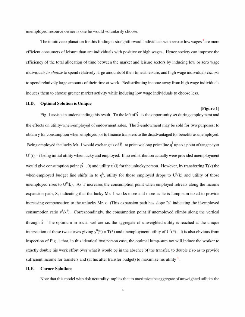
II.D. Optimal Solution is Unique[Figure 1]

Fig. 1 assists in understanding this result. To the left of x is the opportunity set during employment and

the effects on utility-when-employed of endowment sales. The x-endowment may be sold for two purposes: to

obtain y for consumption when employed, or to finance transfers to the disadvantaged for benefits as unemployed.

Being employed the lucky Mr. 1 would exchange z of x at price w along price line qiup to a point of tangency at

U1(i) -- i being initial utility when lucky and employed. If no redistribution actually were provided unemployment

would give consumption point (x , 0) and utility x0(i) for the unlucky person. However, by transferring T(k) the

when-employed budget line shifts in to qk, utility for those employed drops to U1(k) and utility of those

unemployed rises to U0(k). As T increases the consumption point when employed retreats along the income

expansion path, S, indicating that the lucky Mr. 1 works more and more as he is lump-sum taxed to provide

increasing compensation to the unlucky Mr. o. (This expansion path has slope "s" indicating the if-employed

consumption ratio y1/x1). Correspondingly, the consumption point if unemployed climbs along the vertical

through x. The optimum in social welfare i.e. the aggregate of unweighted utility is reached at the unique

intersection of these two curves giving y0(*) = T(*) and unemployment utility of U0(*). It is also obvious from

inspection of Fig. 1 that, in this identical two person case, the optimal lump-sum tax will induce the worker to

exactly double his work effort over what it would be in the absence of the transfer, to double z so as to provide

sufficient income for transfers and (at his after transfer budget) to maximize his utility 4.

II.E. Corner Solutions

Note that this model with risk neutrality implies that to maximize the aggregate of unweighted utilities the

9

"lucky" worker might be lump-sum taxed all the way back to the origin, where he allocates his entire endowment

to work so that z = x and his entire earnings are transferred away so that T = wx. This in turn implies that the

lucky worker may run out of earnings altogether before marginal utilities can be equalized. In this case a corner

solution is reached with Mr. 1 at the origin after transfers and Mr. o on the vertical through x but short of the

point of its intersection with the income expansion path/ray "S". When there are equal numbers of lucky and

unlucky individuals, such a corner could only be reached if w < s. As is easily shown s > w if and only if the

supply of labor z(w) > (x )/2; in other words if and only if more than 50% of the endowment is offered for sale.

Such a high proportion may be implausible for individual labor supply though less so for small countries

supplying an export product. However, this crucial or cutoff proportion z(w)/(x ) -- which determines whether

optimal distribution will press the lucky, employed individuals to a corner -- declines as more are unemployed in

proportion to the "lucky" employed. For example, if there were two identical unlucky individuals of "type-o" and

one lucky one of "type-1" then the necessary condition for optimal redistribution to go to a corner is that s > w/2,

and this in turn requires z(w) > (x)/3. The condition generalizes to nw < ms where n indicates the number

employed, and m the number unemployed; correspondingly, a corner solution therefore requires z(w) > x

[n/(n+m)], where n/m represents the ratio of lucky to unlucky individuals. Thus, the higher the ratio n/m the

higher must be z(w)/x for optimal distribution to push the lucky to a corner solution.

II.F. Welfare Effects of a Wage Increase

This in turn raises the question of the effects of an increase in wage on the post transfer welfare of the

lucky worker, who increases his work effort as a result of the lump-sum tax -- actually doubles his work effort as

we have seen if he must support one entire unemployed individual (i.e. if n/m = 1). Obviously, the unlucky Mr. o

benefits unambiguously from an increase in w for Mr. 1. The question is whether the lucky individuals benefit

from an increase in their wage after the optimal transfer of income. Insight into an answer may accompany the

observation that if an increase in wage caused no change in pre-tax labor supply, it would cause no change in post-

tax labor supply (which if n/m = 1 is double pre-tax supply) and therefore would increase the lucky person's after

tax measured income without increasing work effort. Thus if the wage-price elasticity of supply of labor is zero,

10

then labor of "type-1" will benefit from a wage increase even after paying the lump-sum tax. This proposition

obviously obtains a fortiori if the pre-tax labor supply is backward bending at the point of a wage increase, since

after-tax consumption of leisure and after-tax measured income both will increase with an increase in wage rate.

However, if the supply of labor is sufficiently elastic, might not the pre-tax labor supply increase so much that

after doubling his work effort so as to provide sufficient lump-sum taxes to the unlucky, the "lucky" worker

actually finds he is worse off as a result of the wage increase combined with the transfer ? We now turn to this

question.

The precise condition for an increase in wage rate to harm the lucky workers follows from the first order

conditions (equations 2 and 3), and linear homogeneity of the utility function. To derive this condition we

introduce additional notation as follows:

n (m) = number of employed (unemployed)

s(w) = optimal consumption ratio y/x;

s(w)x = transfer of y received by each unemployed or unlucky individual required tto effect a social optimum assuming an interior maximum

sw = Ms(w)/Mw = (s/w) σ

σ = elasticity of substitution in consumption;

z(w) = optimal labor supply as a function of w if no lump sum transfers acrossindividuals or contingencies were made;

z(w)(n+m)/n = optimal labor supply of each lucky individual -- allowance made for work

required to pay for optimal transfer to unlucky people;

wz(w)(n+m)/n = gross earnings of lucky people before their payments of transfers;

(m/n)s(w)x = transfer payments from each lucky working person needed to transfer s(w)xto each unlucky unemployed person;

zw = Mz(w)/Mw

With "n" lucky-employed individuals and "m" unlucky-unemployed individuals then for each dollar collected from

the n lucky n/m dollars are received by each unlucky person. Therefore, the welfare of the lucky, after the

optimal transfer has been paid and assuming an interior solution becomes:

(4) 1 1 ˆ ˆU = U [[x - (n+m)/n)z(w)], [((n+m)/n)wz(w) - (m/n)s(w)x]]

11

The effect of an increase in wage on post transfer utility of the lucky working person is found from differentiating

equation (4) with respect to wage. This yields:

(5) 1 1 ˆ[( ) / ] [{[( ) / ][ ( ) ]} ( / ) ]X W Y W WdU dw n m n U z U n m n z w wz m n xs= − + + + + −

Then substituting 1 1/X Yw U U= from the first order conditions;

(6) 1 ˆ[ [( ) / ] [{[( ) / ][ ( ) ]} ( / ) ]Y W W WdU dw U n m n wz n m n z w wz m n xs= − + + + + −

As in the usual case, the value of income earned from the increase in labor supplied just offsets the value of leisure

foregone, so that (6) simplifies to:

(7) 1 ˆ[[( ) / ] ( ) ( / ) ]Y WdU dw U n m n z w m n xs= + −

Thus, the welfare effect boils down to whether the increase in earnings on infra-marginal labor supply is sufficient

to pay the extra transfer required. From equation (7) it might appear that a large labor supply -- by making the

increment to infra-marginal earnings due to a wage increase correspondingly large -- would indicate a greater net

gain to the lucky from such an increase in wage. This would be mistaken however. For substituting sw =

Ms(w)/Mw = (s/w) σ and s/w = [wz/[w(x - z)]] gives:

(8) 1Y ˆ ˆ ˆdU/dw = U [[(n+m)/n]z/x - [(m/n)z/(x - z)] ]xσ

Thus, other things equal (given values of m, n, and σ) a large labor supply increases both infra-marginal earnings

for the employed and it also increases the required transfer payment. For a given substitution elasticity the

negative effect on the required increase in transfer outweighs the positive effect on infra-marginal earnings. Thus

the condition for an increase in wage to cause a benefit versus a loss to the people who receive it can be written

(9) >ˆ ˆdU/dw 0 [(x - z(w))/x] {m/(n+m)}

<σ>

↔<

Ceteris paribus a lower substitution elasticity means a lesser increment in the transfer required and therefore a

higher gain (lesser loss) for the lucky-employed, while a lower supply of labor also reduces the required transfer

proportionately more than it reduces the inframarginal gain from which such transfers will be made. This bizarre

effect states that a wage increase may make an unemployed person so much more efficient a consumer of goods

12

that those employed must work very much more to provide sufficient income to the unemployed -- so much more

that those employed actually suffer from a wage increase 5.

The above analysis is automatically generalizable to n different goods with given relative prices, as long as

these relative prices are unaffected by lump-sum redistributions. For then Hicks's Composite Good Theorem

implies that we can aggregate all such goods into a single composite.

III: RESOURCE UNEMPLOYMENT AND OPTIMAL INSURANCE

One important generalization of the foregoing analysis extends to the optimal distribution of

income among contingencies! Just as first best lump-sum redistributions across people will reverse the order of

utilities, the same is true across contingencies for the same entity (or for different ones). Many instance of the

reversal theorem fall into this category; the resource owner who can sell some or all of his endowment at in good

times, but be cut off from his market entirely in bad; the worker facing a risk of unemployment; the country facing

a risk of trade disruption; the Rawlsian citizen confronting a risk of disability. As in the optimal tax problem the

reversal paradox is acknowledged in the insurance and particularly the labor contract literature 6, but has not been

analyzed for itself 7.

III.A. The Equivalence Between Lump-sumTransfers and Fair Insurance

The essential equivalence of these two transfer problems can be illustrated if we ask how much

consumption is it rational to transfer between contingencies via insurance purchase. One benchmark exchange

rate between contingencies is the "fair price," the price at which expected benefits equal expected costs, or

expected monetary gain/loss is nil. An ability to transfer income between contingencies at fair prices is equivalent

to an ability to lump-sum transfer income. And when fair insurance is available, the rational resource owner if he

is risk neutral (or risk averse 8) will necessarily over insure, so much that the otherwise "bad" contingency becomes

preferred 9. Using the same innocuous assumptions of (a) two goods,(b) two contingencies,(c) fair insurance, and

(d) risk neutral, state independent linear homogeneous utility, this result follows from the necessity that when

markets are incomplete an optimizing subject must trade off the benefits from an optimal commodity mix under

13

alternative contingencies against unequal levels of utility in the alternative states of the world 10. It depends in no

way on arguments from moral hazard (Pauly 1968) 11. Nor does it involve any presumed ability to protect against

unemployment by probability improving "self-protection" measures (Erlich and Becker, 1972), nor interactions

between these and risk aversion (McGuire, Pratt and, Zeckhauser, 1991). On the contrary, in the case to be

studied here the probability of trade cutoff or unemployment is completely fixed.

III.B. Assumptions

The assumptions for this intercontingency analysis strictly parallel those for optimal income distribution

12. In this version of the problem the agent acts so as to maximize the expected value of a Von Neumann-

Morgenstern expected composite utility

(10) 1 0W = pU ( ) + (1-p)U ( )

where p, probability of employment and (1-p) that of unemployment are known and fixed. He can protect himself

against loss of y-consumption if unemployed by paying out a premium which costs t = (1-p)b/p when (or if)

employed. In return he receives insurance benefit b if unemployed. Since (1-p)b - pt = 0 this insurance is

actuarially fair.

III.C. The Optimal Insurance Purchase

Theorem: As with interpersonal transfers, at the maximum of W = W(*) -- where "*" indicates

solution values -- U0(*) > U1(*) , provided f " = 0 throughout. To maximize his expected utility, this agent will

purchase so much fair insurance that he is better off if the "bad" event is realized and he collects his insurance

benefit. This follows from the first order conditions for maximization of

(11) 1 0ˆ ˆW = pU [(x - z), (wz -{(1-p)b/p})] + (1-p)U [x, b]

with respect to z and b. The FOC's are the same as those for the optimal redistribution problem:

(2 repeated) 1 1X Y- U + wU = 0

(3 repeated) 1 0Y Y- U + U = 0

Where Ukh indicates the marginal utility of good h in state k 13.

For risk neutral linear homogeneous utility [f(V) = U = B V] equalization of the marginal utility of good y

14

across contingent states means again that the marginal utility of x must also be the same across contingencies, and

therefore following the same argument as made in the interpersonal redistribution case x0(*) > x1(*) and y0(*) >

y1(*). With consumption of both commodities higher under unemployment than employment, utility must be

higher in the former state 14. [FIGURE 2 HERE]

Again the rational resource owner will insure or save so much that in the bad state of the world he would

choose not to trade his resource even if he could (which he can not of course). As in the interpersonal transfer

case, the optimal preparation for unemployment is to provide so much that in the event one would choose not to

work 15..This result is pictured in Fig. 2 --- similar to Fig. 1 with an addition to the right of the vertical through x .

Now the x-endowment may be sold for two purposes: to obtain y for consumption when employed, or to pay

insurance premiums (or savings) for benefits if unemployed. To the lower right of x the fourth quadrant of the

diagram shows the intercontingency transformation of premiums into insurance reimbursements at fair-odds

prices. 16. If no insurance were purchased under conditions of employment, exchange of x at price w would be

pursued along price line qo

up to a point of tangency at U1(i) -- i being initial utility when employed, and

unemployment would give consumption point (x , 0) with utility U0(i). However, by spending t to purchase b of

insurance at the fair price of t = [(1-p)/p]b the employment line under the good contingency shifts in, utility if

employed drops and utility if unemployed rises. As t and b increase the consumption point when employed

retreats as before along the income expansion path, S; and the consumption point if unemployed climbs along the

vertical through x. The optimum in expected utility is reached at the unique intersection of these two curves

giving y0(*) = b(*) and unemployment utility of U0(*).

III.D. Benefits and Costs of Insurance

A complementary way to summarize this result is to calculate the costs (measured in expected utility terms) of

insurance premiums expended as the reduction in V1 = U1 weighted by p, while the benefit (again in expected

utility terms) from insurance benefits received is calculated as the gain in V0 or U0 weighted by (1-p). With U = B

V, and V a CRS function, the weighted cost is linear as consumption-when-employed retreats along ray S, and

therefore expected marginal utility cost is constant. On the other hand, the probability weighted utility gain is

15

diminishing as consumption-when-unemployed climbs the vertical through x 17. Thus expected marginal benefit is

uniformly decreasing and the optimal insurance purchase is uniquely determined.

III.E. Comparisons of Income andConsumption Across Contingencies

Figures 3a. and 3b. show the same effect with the inter-contingency consumption opportunity frontier, and

utility possibility curve. As the risk neutral subject buys insurance at fair odds to transfer goods-consumption from

the good to bad outcome his he gains [p/(1-p)][(s+w)/s] in y0 for each t = 1 unit of y he gives up. Note that the

resource owner offsets some of the loss in y1 consumption (i.e. the costs of insurance premiums) by working more

(or increasing his production of y1). Therefore the trade-off between goods-consumption in the two contingencies

is superior to a fair odds trade off, and the slope of the inter-contingency goods-transformation curve in Fig. 3a is

flatter than and superior to fair odds. As the subject buys small amounts of insurance, first he will achieve equal

utility across contingencies. The utility gain from the insurance benefit is great because it is combined with the

subject's resource (all of which is available when the market is lost). This allocation falls far short of maximization

of expected utilities since at such an iso-utility allocation, the marginal utility of goods-consumption is greater in

the bad than in the good state of the world. After this iso-utility allocation is reached, further insurance purchases

yield an iso-commodities-consumption allocation, where the amount of measured y-income is the same across

contingencies. Expected utility is still not maximized since with y1 = y0 and x0 > x1 the marginal utility of y is still

greater in state "o" than in state "1". Accordingly, Fig. 3a and 3b show the tangency maximum in expected utility

to the right of both the iso-utility and the iso-goods-consumption points. [Figures 3a & 3b]

III.F. Corner Solution Limits on Insurance

It follows from the construction of Fig. 2 that under risk neutrality, the optimized (insurance protected)

unemployment utility is unaffected by the probability of unemployment provided resource allocations to insurance

do not force a corner solution. For lower values of p -- i.e. lesser likelihood of uninterrupted trade, or employment

-- the optimized value U0 (*) remains unchanged with the entire utility deficit absorbed by lower and lower values

of U1 (*) 18.

16

Proof: From homogeneity with V1Y(*) = V0

Y(*) the unemployment and employment consumption

bundles lie on the same ray through the origin; but the unemployment consumption bundle must lie on the vertical

through x . The intersection of these two lines is unique and independent of p.

Corollary: As the probability of unemployment 19 increases from zero, gross earnings when employed

(inclusive of insurance premiums) rise monotonically; insurance premium payments rise monotonically at a rate

faster than the rise in earnings; and the proportion of gross earnings replaced declines monotonically from

[(s+w)/sw] to [s/w] as p declines from p = 1 to p = p where w = wage rate, or sales price of exports, and s = slope

of income expansion path at wage-price w, and p is as defined next.

Corollary: For every value of s there is a value of p = p which induces the risk neutral consumer

insuring at fair odds, to allocate his entire earnings-if-employed to insurance premiums. Similarly, for every p

there is an s = s which induces all earnings to be allocated to insurance. Moreover, such an insurer will give up

his entire endowment of x to earn y to buy premiums to cover his unemployment.20.

Proof: By inspection of Fig. 2, for any p, or fair odds line, if s is great enough, y0 (*) = b(*) will be great

enough in turn to require a t(*) which absorbs x in its entirety. It also follows that for the same wage line, the

more industrious the worker, i.e. one with a higher slope s = y/x of income expansion path S will reach this corner

solution at lower risks of unemployment (1-p) than will a less industrious worker. Another way of stating the same

effect is to say the higher the wage, at any given risk of unemployment, the greater will be the proportion of gross

earnings allocated to insurance.

III.G. Welfare Effects of a Wage or an Export Price Increase

The effect a rise in the price of the resource, as in the case of optimal income distribution, may increase or

decrease the supply of the resource (labor or export good for example) depending on its supply price elasticity.

However the amount of insurance purchased and therefore the utility in the bad or unlucky state of the world will

unambiguously increase with an increase in price. Moreover, with sufficiently elastic supply of the resource, an

increase in price will require an increase in supply so great as to lower net-of-insurance-premium welfare in the

good or lucky state of the world.

17

IV: FURTHER PROPERTIES OF OPTIMAL ALLOCATIONS UNDER RISK NEUTRAL UTILITY

IV.A. Extension to "Unfair" Insurance: Insurance Loading

Fair insurance is rare as is lump-sum income transfer. Insurance providers usually add a "loading factor"

to recover administrative costs, to yield a profit, or anticipate moral hazard or adverse selection. To represent this

effect, let the unit price of insurance be not (1-p)/p which is the "fair" price, but instead [{(1-p)/p}r +g]. This

adjusts the fair price by a fixed unit charge "g" and a proportional risk inflator,"r." With this adjustment the

necessary conditions for an expected utility maximum become

(12) 1 1X Y- U + wU = 0

(13) 0YU - p[((1-p)/p)r + g]/(1-p) = 0

[Figure 3c]

If "g" in eq. (13) is zero and only the risk-inflation factor enters, the change compared to fair insurance is

slight. (a) The optimal purchase (receipt) of insurance remains fixed independent of p, though at a lower amount

than with fair insurance. (b) It no longer seems possible a priori to assert that welfare when unemployed is

necessarily greater than when employed; the outcome can tip either way depending on the ordinal utility function.

However, if earnings net of the insurance premium are fully replaced or more it is clear welfare is higher in the

unemployed state; and it is clear moreover that the higher the likelihood of unemployment the more probable will

this be true, since earnings in the good state decline with greater (1-p) while ex post consumption in the bad state

is unaffected.. (c) Similarly, as in the no-load fair insurance case, when the probability of unemployment (1-p)

rises, unemployment utility is unaffected (though it reaches a lower level than in the fair insurance case) and the

entire burden is allocated to the state when employed. (d) Likewise more industrious individuals will allocate a

greater share of their earnings to insurance premiums than will less industrious.

A positive value for loading factor "g" changes the analysis lending another sort of

predictability. For now as the probability of unemployment increases and p declines, the actuarial cost of the

fixed load g is recovered with increasing likelihood (spread over a larger set of contingencies) so that the

amount of insurance purchased increases as p declines. Pictorially, with g > 0, as p declines the optimal

solution point ascends the vertical through x, approaching the solution with g = 0

18

Now the seller of insurance can counteract this tendency driven by the rationality of greater insurance

purchase with greater risk, by making/causing r (the inflation factor) or g (the fixed load factor) or both of these to

change with risk. But analysis of such a game between buyers and sellers would take us beyond our focus here.

IV.B. Insurance Against A Demotion, Terms ofTrade Reversal, or Partial Disability

We have been concerned with an individual who earns nothing, a country which is totally embargoed, a

Rawlsian citizen born completely disabled, or retirement which allows no gainful employment whatsoever. What

of the case where the "bad" outcome is less extreme? Rather than total unemployment, the worker is demoted to a

lower wage job; rather than an embargo a country risks adverse developments in its terms of trade; rather than total

disability the celestial citizen contemplates diminished opportunity; and the retiree can pick up odd jobs at a

lessened wage? How does enriching and softening the scenario for the "bad" outcome, alter the result? The

answer is that we can generalize the foregoing analysis not only to differences in wage rates caused by differences

in ability, but also differences in the effective prices paid for different goods by different individuals. Perhaps

some individuals are more efficient searchers than others, or have more efficient household production functions.

Individuals who are more efficient at producing a particular good, and therefore experience a lower effective price

for that good would have a higher level of initial utility than less efficient individuals. As long as the good has a

positive income elasticity, marginal utility of income is lower to the more efficient individuals when the level of

utility is the same for all. Consequently, a lump-sum transfer or fair insurance purchase would also reduce the

utility level of the more efficient below that of the less efficient in this case as well.

To be more specific suppose the bad outcome is a reduction in wage from w1 in good times to w0 in bad

times. This situation is pictured in Figure. 4. Now the expected utility maximand becomes: [Figure 4]

(14) 1 1 1 0 0 0ˆ ˆpU[(x - z ),(w z - {1-p}b)] + (1-p)U[(x - z ),(w z + pb)]

with variables of choice now work effort in each of the two states z1, zo, and insurance b. For interior solutions

the necessary conditions become

(15) 0 0X Y 0U (*)/U (*) = w

(16) 1 1X Y 1U (*)/U (*) = w

19

(17) 0 1Y YU (*) = U (*)

However, all three necessary conditions cannot be satisfied at once unless w1 = w0 ; but the essence of the problem

lies in the assumption that the two wages differ. The last condition requires equal marginal utilities of good y (and

by inference under CRS utility of good x as well) across contingencies. But this is inconsistent with unequal

marginal rates of substitution as required by the first two conditions when w1 ≠ w0. Accordingly, the expected

utility maximizing individual either can purchase optimal insurance with an outcome at the intersection of the

vertical through x and the consumption ray with slope s1, or must settle for sub-optimal insurance due to his

resource limits. If optimal insurance is available, the rational individual will refrain from working at all at the

lower wage w0. If the only insurance available is inadequate, however, then the individual may have to depend in

part on the safety net provided by work at the lower wage.

V: EXTENSION TO RISK AVERSE AND RISK PREFERRING UTILITY

V.A. Risk aversion: f '> 0, f " < 0

To address the effect of risk aversion we will employ an extension to multi-commodity situations of the

Arrow-Pratt (1963, 1964) definition of risk aversion as proposed by Kihlstrom and Mirman (1981) viz. a concave

transformation of the common utility function V(xj,yj) representing the same ordinal preferences across

individuals or contingencies. The "underlying" linear homogeneous function, V, is not altered; the same ordinal

rankings and indifference curves as in Figs. 1 or 2 apply, except now these are renumbered. Each indifference

curve, by strict quasi-concavity, has strictly a diminishing marginal rate of substitution (MRS). The necessary

condition for a maximum to replace eq. (3) can be written

(18) 1 1 1 0 0 0Y Y-[f '(V )][V (s )] + [f '(V )][V (s )] = 0

With V, first degree homogeneous, its first partial derivatives are functions of the consumption ratios, yk/xk = sk

only. (Since this is important in the argument to follow, the dependence is shown explicitly).

To show that U0 (*) > U1(*) after optimal insurance has been purchased at fair odds, now assume U0 (*) <

U1(*) contrary to what is to be proved. Note that the indifference curve through [x1(*),y1(*)] --- being convex with

negative slope -- intersects the vertical through x , at a lesser value of s than s1. Therefore, the value of s0 is still

lower for a lower indifference curve V0 < V1 . Therefore, if V0 < V1 it follows that s1(*) > s0(*). In turn this

entails V1Y(*) < V0

Y(*). Whence to maintain eq (18), f '[V1(*)] > f '[V0(*)]; this in turn entails V0(*) > V1(*),

20

which contradicts U1 (*) > U0(*). Thus if f ' > 0 and f " < 0, U0 (*) is strictly greater than U1(*). QED.

Intuitive support for this conclusion might begin by considering an allocation which yields the same

value of V equally or irrespective of which state of the world occurs, i.e. the value of V = V1 = V0 at this

allocation the marginal utility of benefits vs. the marginal cost of further incremental insurance is determined

strictly by the consumption mix, y0/x0 < y1/x1. With V0 = V1, then at this trial allocation f ' [V0 ]= f ' [V1]. But the

consumption mix strictly favors adding y to state "o"; therefore, an iso-utility allocation cannot be maximal.

However, for further insurance beyond this trial value where U0 = U1 the concave transformation of V changes the

probability weighted marginal utility cost of insurance from a constant to an increasing function of the amount of

insurance provided, and at the same time accelerates the decline of the marginal benefit function. The upshot of

these two effects is that risk aversion reduces the equilibrium insurance purchase below the risk neutral level but

not so much that unemployment becomes less desirable than employment.21

V.B. Risk preference; f ' > 0, f" > 0

The potential for multiple optima inherent in the non-convexities introduced by risk preference shows up

pointedly in this analysis as well. Compared with the risk neutral outcome, a positive convex transformation f(V)

can lead to two types of alternative solution. Imagine starting from the risk-neutral optimum (with U0(*) > U1(*);

then increase f " slightly from zero. One possible effect is for more insurance to be purchased and the superiority

of "bad" over "good" luck to increase. A second is that risk preference requires purchase of less fair insurance-- so

much less that unemployment is not fully insured and remains the less desirable outcome. [Figure 5]

In the former case the unemployment consumption point moves up the vertical above the risk neutral

y0(*) = b(*). In this region U0(*) > U1(*), s0(*) > s1 (*) and UY0(*) < UY

1(*). Consistency with eq. (18) requires f

' 0 > f ' 1(*), and, therefore, risk preference in the utility function, f " > 0. Alternatively, consumption when

unemployed can move below the risk neutral y0(*). In this region, s0(*) < s1(*). and, therefore, UY0(*) > UY

1(*).

In this case, consistency with eq. (18) requires f ' 0 < f '1(*). Thus if f " > 0 then V0(*) < V1(*). Fig. 5 shows both

cases. There the probability weighted underlying function of benefits and costs -- V from the risk-neutral case --

has been subjected to a convex transformation through the point where U0 = U1. This increase in f " causes the

probability weighted marginal utility cost to change from constant to declining, and the weighted marginal utility

benefit to decline more rapidly. The possibilities for multiple solutions are clear.

21

VI: MORAL HAZARD

But if the case for over provision or over insurance is as logical as the foregoing argument suggests, why

does it seem rarely observed? One reason may be that such optimal provision for adversity interacts with moral

hazard. Should insurance proceed so far that bad fortune turns to good, the temptation to court the bad outcome

may be irresistible.22

Moral Hazard Neutralized By Fair Insurance PricingCombined With Costless Re-contracting

To illustrate consider one agent who can insure himself against mishap at a perfectly fair price. Our

analysis tells us he will always buy enough insurance so that in the event of misfortune his consumption of

0 ˆy (*) = sx . With fair insurance this requires a premium payment of ˆ[(1 p) p]sx− . It follows 23 that

optimal expected utility, optimized by purchase of fair insurance can be written:

(21) 1 0(1 )ˆ ˆ ˆ ˆ( ) [{ (1 )},{ ( )}] (1 ) ( , )

( ) ( )

s ws p sV p pU x x p U x sx

p w s p w s p

−= − − + −

+ +

Now to start let the agent be free to choose p, knowing that whatever his choice he can buy fair

insurance. Once p is chosen and insurance is purchased, however, suppose the agent cannot cheat. Then the

writer of insurance earns zero profit but by assumption is protected from moral hazard. To derive the insured

agent's optimum note that the values of x, s, and w are all taken as parameters, so that the last term U0 is

constant. Then first order conditions for an optimum require

(22)1

1 0( )0

dV p dUU U p

dp dp= − + =

(23)1 2

1 1ˆ ˆ

( ) ( )X Y

dU xs xsp U U

dp p w s p w s= +

+ +

Then using the FOC 1 1X YU wU= gives

(24)1

1 1ˆ ˆY X

dU xs xsp U U

dp p pw= =

The underlying utility function is linear homogeneous. Suppose it is 1U x yα α−= ; then along income

expansion paths / (1 ) /s w α α= − . Next, define 1 1[{1 ) / } ]s wα αα α β− −= − = . Then 24 for dp > 0

22

(27)1

0 1 ˆ ˆ 1[ (1 )] [ (1 )] 0

{ /(1 )} 1

dU x s xU U p

dp p w s pα β α β

α α− + = − + − = − + − =

+ − +

Thus the rational and perfectly and fairly insured agent with homothetic utility and deprived of all opportunity to

cheat (i.e. to alter the value of p he has chosen after he has bought insurance) is indifferent among outcomes 25.

Although he has no reason to take any action to avoid risks, neither has he any incentive embrace risk, provided he

is not driven to a corner. In a space of U0 - U1 his utility possibility curve is a straight 45O line. This establishes an

entry point for considering the moral hazard problem under our assumptions.

The opportunity to insure fairly induces indifference to risk in his behavior, since unit costs (in terms of

utility foregone in the good outcome) are constant (short of corner solutions) and thus this opportunity neither

promotes nor suppresses moral hazard, since neither the buyer nor the maker of the insurance loses anything here.

If the maker writes a fair insurance policy and can always re-contract if p changes, he is compensated for otherwise

unfavorable changes in p. And for the buyer of ideal insurance), if changing his risk profile can bring in money

then he will simply economize with a choice of risk that maximizes this source income. Whether this would

involve greater caution or less for him is irrelevant since he can insure.

In other words, in and of itself, risk is not a "bad thing." Once can see this from allowing resource

expenditures "m" to influence p, so that p =p(m), where m is an "outlay" required in both contingencies. Now in

place of Equation (11) expected utility can be written

(28) 1 0

z, m, bˆ ˆMax : W = p(m)U [(x - z), (wz -m-{[1-p(m)]b/p(m)}] + (1-p(m))U [x, (b-m)]

First order conditions require as before

(29) 1 1: 0X Yz U wU− + =

(30) 1 0: 0Y Yb U U− + =

(31) 1 0 1 02

( 1): [ 1 { } '] (1 ) '[ ] 0Y Y

pm pU b p p U p U U

p

+− + − − + − =

From (30) it follows that ˆb m sx− = . In other words, fair insurance still takes the consumption point (net of

expenditure m) up the vertical through x to the intersection with the income expansion path with slope "s".

Utilizing this inference we could proceed as before,. Solving (29) and (30) for z ---which gives

23

ˆ( ) / ( )z sx m p w s= + + --- and then folding this together with ˆb m sx− = into Equation (28) we could ask, what

now is the optimal value of m and thus of p. We can avoid this effort, however, by recalling that absent p, m and

p(m) the rational agent is indifferent among values of p. This must mean that the optimal m in (28) is either zero

or negative. With no payoff to p' itself (as we have established) its value can only be instrumental. Thus if m is

negative, our agent is compensated for taking risks. But since he is indifferent to risk itself because he is perfectly

insured, he will seek the maximum in compensation. He wants to maximize -m > 0.

At this optimum the inverse function m = m-1(p) will have zero first derivative. Moreover with -m at this

maximum, the rational agent will have minimized the amount of fairly priced insurance purchased. The positive

compensation -m, lifts his endowment point at the bad contingency above point ˆ ˆ( ,0) to point ( , )x x m− , so that to

consume at ˆsx in "bad" times he wants/needs to insure less.

This reasoning in no way undermines the qualitative conclusion suggested by our analysis, that an agent

say the size of an entire country should write self-insurance by stockpiling significant amounts for emergencies,

especially if it can self insure at actuarially fair rates. The larger the size, the more plausible is fair self-insurance.

However, this might occur over lengthy periods of time 26, so that the process (aside from any other resources

costs of stockpile accumulations and maintenance) should have to reckon with interest expense (implicit or

explicit), and this could modify the neutralization of moral hazard just identified.

Incentives Under More Realistic InsurancePricing and Informational Assumptions

Introducing more realistic insurance-pricing and information assumptions, even with homothetic, risk

neutral utility raises further interesting questions concerning the question of moral hazard. Suppose that rather than

actuarial fairness, the price paid in the lucky contingency to obtain one unit of good-y in the unlucky contingency

is as in Equation (13) above, i.e. [{(1-p)/p}r +g]. Such insurance premium "price loading" implies optimal

consumption in the bad contingency below 0 ˆy s x= But there is an interesting novelty here as Eq. (13) shows:

the greater the risk of the bad contingency --- greater (1-p) --- the more of the income shortfall (i.e. of the distance

s x) will be replaced, and the closer will the solution U0* approach the fair insurance outcome. The reason is that

as p increases the constant load "g" recurs with greater likelihood and the effective actuarial cost of insurance

increases, so less insurance is bought. Accordingly, to avoid/spread the fixed cost, the insured entity desires low p

i.e. greater risk, a sure moral hazard incentive. This train of thought implies that pricing insurance as per Eq. (13)

24

[{(1-p)/p}r +g] is a bad policy for the writer of insurance since it provides incentives to the insured party to

minimize p --- aside from any other costs or benefits incident to choice of p germane to that insured party.

Assumedly this effect is well established in the theory and practice of insurance writers, and has caused insurers to

reject simple formulas like [{(1-p)/p}r +g] and for example to limit amounts of insurance purchasable, or to

monitor risk histories and behaviors.

If the assumption of costless re-contracting is discarded the interactions between insurance and incentives

to cheat are still more striking, as is demonstrable with the following thought experiment. Suppose p is fixed and

fair insurance is offered/purchased as per Eqs (11, 2, and 3), and illustrated in Figure 2. Now holding insurance

premiums and the outcomes U0* and U1* fixed (i.e. no re-contracting by the insurance writer) allow the agent to

cheat by choosing a different value of p. His optimum is obviously p = 0; then he enjoys U0* throughout. Next

suppose the agent anticipates the opportunities to cheat after insurance is written/purchased. Now in anticipation,

how much insurance will he buy? Obviously, if he can make p = 0 after he has purchased insurance at some

positive value of p = p*, he will allocate his entire income/effort to insurance purchase, pushing his consumption

in the "bad" contingency as high as possible above the intersection of s with the vertical through x identified in

Figure 2, and choosing a consumption point in the "good" state of x = y = 0, at the origin of diagram 2. It seems

that linear homogeneous utility combined with the opportunity to purchase insurance at a fair price knowing you

can cheat afterwards, dramatically increases ones incentive to cheat.

VII CONCLUSION

The problem sketched out here is representative of a broad class of situations in which individuals or

groups are at risk of being thrown back on their own resources and cut off from exchange with nature or with other

persons or institutions. The main insight from the analysis is that rationally desired provision against the loss of a

market for one's resources can easily be great enough to cause "over" insurance or "over" protection --- where the

desirability of the good and bad outcomes is reversed. In fact this is the expected case. No matter how risk averse

the subject, if he can make "fair odds" provision he will protect himself so much that he prefers the state "loss of

market plus benefit" to the state "regular earnings minus savings". If this effect were more broadly recognized

than it seems to be, and the incentives it can imply for moral hazard more widely recognized, the so called

disincentive effect of unemployment benefits might seem less perverse and deplorable, the argument for dramatic

transfers to the disabled might seem to require much less altruism, the arguments for stockpiling taken more

25

seriously, and the need for monitoring against cheating more urgent.

26

FOOTNOTES

* ACKNOWLEDGEMENTS. This paper was delivered to the Memorial Conference in Tribute to Jack

Hirshleifer, Department of Economics, UCLA, March 10-11, 2006. We thank Philip Cook, Bill Evans,

Arnold Harberger, David Hirshleifer, Karla Hoff, Hiroyuki Kawakatsu, Kai Konrad, David Levine, Leonard

Mirman, Mancur Olson, and Mark Pauly for helpful comments on this and on earlier versions.

1. Of course a country anticipating cut off from foreign markets might contemplate other measures than taking out

insurance (via agreements with allies supposedly). For instance it might, if feasible, stockpile the import at risk.

Similarly, the individual at risk of involuntary unemployment might prepare an alternative individually productive

use for his surplus leisure. Alternatives like these may approximate insurance purchase under some circumstances

(McGuire, 1990, 2000).

2. The cases representing risk aversion or risk preferring utility in which f(V) is any positive smooth

continuous concave or convex transformation with continuously increasing or decreasing first derivatives

will be dealt with presently in Section V.

3. Section IV of this paper extends the above analysis of redistribution between individuals with positive

and zero wages to redistribution between individuals with low and high wage rates. Our characterization of

the intuition of our result anticipates this extension.

4. In Fig. 1 the distance ab must equal distance xT(*) to transfer the amount T(*). Therefore, the triangles

with bases ab and xT(*) are congruent and of equal height.

5. Another way to look at the same effect is to compare the shape of the indifference curve which passes

through the post-transfer consumption point of the lucky-employed person, with the opportunity curve which

passes through the same point and describes his consumption path as wage varies. Let ‹[x(w),y(w)]

indicate that opportunity set where x = [x - {(n+m)/n}z(w)], and y = [{(n+m)/n}wz(w) - (m/n)s(w)x]. The

slope of this opportunity curve is

27

(9a) ˆ[{[( ) / ][ ( ) ]} ( / )

[( ) / ]w w

w

n m n z w wz m n xsy w

x w n m n z

= + −∂ ∂= −

∂ ∂ +

and the slope of the indifference curved is - w. Therefore utility declines if the opportunity curve has a

smaller negative value than - w, i.e. if

(9b) ˆ[{[( ) / ][ ( ) ]} ( / ) ]

[( ) / ]w w

w

n m n z w wz m n xsw

n m n z

= + −− > −

+

which occurs if

(9c) ˆ [ /( )]x x m n m σ< +

which is the same result as (9) above.

6. Such would include analyses of employment contracts (such as Milgrom, 1988), unemployment insurance (e.g.

Shavell and Weiss, 1979), or stockpiling of imports subject to embargo (e.g. Tolley and Wilman, 1978; McGuire,

1990) and the immense literature on provision for retirement. We emphasize that buying insurance may be only

one of many possible protective measures against risk of unemployment. Others might include stockpiling, limited

autarky, efforts to change the probabilities of bad outcomes or the analysis of the "perverse" incentives afforded by

unemployment insurance (Feldstein, 1974).

7. The closest relative to this paradigm we have found in the literature is the case of insurance against the

loss of an "irreplaceable asset" as analyzed by Cook and Graham (1977). The phenomenon considered here

although kin to that of Cook and Graham differs from them in that we are considering the case of being

deprived of all replaceable assets and thrown back on one inalienable asset -- e.g. time, domestic resources,

seat at the celestial convocation (i.e. claim to existence in some incarnation or other) etc. -- almost the exact

converse of Cook and Graham (1977).

8.The proof as it relates to risk averse utility will be reserved for section IV.

9. This conclusion contrasts with that of Cook and Graham (1977) who conclude that only if the

"irreplaceable asset" is inferior will the expected utility maximizing decision maker over insure.

10. We thank Mark Pauly for pointing out that this result reflects the Arrow-Debreu theorem that for Pareto

28

efficiency the number of markets must equal or exceed the number of contingencies plus goods.

11. Those arguments hinge on the incentive insurance may provide a subject to take less care thereby raising the

chance of the bad outcome, which he has insured himself against, but benefiting from the savings in effort on self

protection.

12. The agent also might be assumed to possess a positive and inalienable but indefinitely small endowment of

good y. This assumption is made to insure that the agent's utility is still defined even after all opportunity to sell

(part of) his x-endowment is prevented.

13. The reason these conditions are identical is that the opportunity to purchase fair insurance produces a price for

inter-contingency transfer which cancels out the probability weights in the expected utility maximand. Or if we

took values of p = 1/2 the maximands of equations (1) and (4) would be precisely the same.

14. The direct analogy between this model and that of saving for retirement in the absence of bequest motive

should be mentioned. Saving from earned income during n working years so as to enjoy one's entire endowment

of leisure during m retirement years has exactly the same structure as the insurance problem with p = n/(n+m).

With state independent, linear homogeneous utility, together with the other assumptions specified in the foregoing

analyses (plus zero bequest motives), the rational planner will save so much that his income/leisure ratio in

retirement is the same as during his working life. As a result consumable commodity income is much greater

during retirement when the entire endowment of leisure is consumed than it is during years of work.

This result is easily established for the individual with n certain years of working life followed by m

certain years of retirement. During each working year his utility is U[(x - z),(wz - t)] ; while during each

retirement year is utility is U[x,b]. Assume a pure year-to-year rate of time preference of i and a marginal rate of

productivity of i. The individual's utility maximizing consumption profile then calls for equalizing marginal

utilities of x and of y across outcomes. With CRS utility this can only result where y/x is the same when working

and retired.

15. This analysis might be challenged as unrealistic because eq. (11) represents only one period, and, therefore,

seems to confuse stocks and flows. In practice insurance premiums are paid in the present for multiple

29

contingencies in the future. Changing the model to a more realistic, multi-period framework, however, does not

alter our main conclusion. Provided one maintains the assumptions that (1) insurance is fair, (2) utility is linear

homogeneous, (3) inter-temporal discounting is ignored it still follows that an interior optimum requires

equalization of marginal utility of goods in all states/contingencies.

Now to consider a two period/two contingency problem in place of (11) we would write the maximand as:

(11a) k k k 1 1 1 0ˆ ˆ ˆW = U [(x - z ), (wz - b)]+pU [(x - z ), (wz +b})] + (1-p)U [x, b]π .

Here, index "k" denotes the present when there is no uncertainty, and as before "1" and "0" the future with two

contingencies. The unit cost of or premium for one unit of benefit "b" is written as "π" Absent discounting,

welfare is the un-weighted sum of the certain present plus expected future utilities. Differentiation with respect to

1( , , )kz z b gives:

(11b)

k

1 1 1

1 0

z : 0

z : 0

: (1 ) 0

k kX Y

X Y

kY Y Y

U wU

U wU

b U pU p Uπ

− + =

− + =

− + + − =

With linear homogeneous utility the first two conditions imply 1 kY YU U= . And if insurance is "fair" and

discounting absent it follows that π =1, whence 1 0kY Y YU U U= = . Thus, the requirement for equal marginal utilities

at an optimum persists, though just how welfare is distributed among present vs. future and the good vs."bad"

outcomes changes due to income effects. Obviously, except for differential income effects, the same conclusion

holds if there are many certain periods followed by one uncertain period. We thank Arnold Harberger and David

Levine for raising this question.

16. This "inter-contingency transformation line" could also be useful to analyze the optimal income redistribution

among different people when the numbers of transferors and transferees are different. For n "lucky" payers and m

"unlucky" payees a slope of n/m would show the tradeoff between transfers per giver and receipt per receiver.

Similarly for n years of work and m of retirement, a slope of n/m would show the ratio of annual savings to

30

receipts, ignoring interest accumulations.

17. If the elasticity of substitution r were (a) infinite, or (b) zero and indifference curves, therefore, were (a)

straight lines or (b) sharp cornered, the benefit curve would (a) also be linear or (b) be linear and have a kink at

the benefit limit where the income expansion path and vertical through x intersect.

18. The analog of this result in the interpersonal transfer case is that as more unlucky poor are added to the

population and the ratio of lucky to unlucky declines, the post-transfer utility of the unlucky is unaffected

until the rich are driven to a corner where they work full time and transfer their entire earnings to the poor.

Only after this corner is reached will the poor's post transfer utility decline with increases in their numbers.

19. Analysis of the effects of changes in probability of unemployment on optimal insurance purchase, and on

the utility distribution between the "lucky" and "unlucky" states has an analog in the optimal income

distribution problem as between different individuals. Changes (increases) in probability of unemployment

correspond to changes (increases) in the ratio of "unlucky" to "lucky" individuals.

20. For example with a Cobb Douglas utility function i.e. --- V =xa

y(1--a)

--- the critical value of p = (1-a); for

p < (1-a) the consumer cannot reach an optimum and is confined to the corner where x1 = 0 and y0 < y0 (*). We

thank Leonard Mirman for pointing this out and for the example.

21. The log utility function U = [aLn(x) + (1-a)Ln(y)] gives a good example of risk averse utility in a bi-

commodity world. In this case maximization of

(18a) ˆ ˆp[aLn(x-z) +(1-a)Ln(wz{(1-p)/p}b)] + (1-p)[{Ln(x)} +{(1-a)Ln(b)}]

with respect to z and b yields

(18b)

1 0

1

0 1

(*) (*) (*)

ˆ(*) { /[1 (1/ ) 1/ ]}

ˆ(*) (*)

y y pwz

x x ap p

x x x

= =

= + −

= > Therefore U0(*) > U1(*). Bill Evans suggested this example, similar to Atkinson-Stiglitz (1980, p. 344).

22. This argument, however, does not tell strongly against saving/investing for retirement; in fact, it may

31

provide explanation for large accumulation for old age additional to or alternative to bequest motives.

23. From the assumption of fair insurance 1 ˆ[(1 p) p]sxy wz= − − , whence

(19)

1

1

ˆ[(1 p) p]sxˆ

y wzs

x x z

− −= =

−

And therefore

(20) ˆ* sx p(w+s)z =

24. The definitions and FOC's give

(25)0 1 0 1ˆ ˆ[ ( ) ]

ˆ ; ;( ) ( )

x p w s s xsU x U U U

p w s p w sβ β β+ −

= = − =+ +

(26)

11 1 1ˆ ˆ ˆ ˆ(1 )

(1 ) (1 )X X

dU xs x x xp U U s

dp pw p p pαα α α β

α−−

= = = − −=

25. This result is not new. Atkinson and Stiglitz (1980, p. 346) draw a linear utility possibility curve.

26. The effect of time, interest, and discounting on the optimal stockpile is discussed in McGuire (2006).

32

REFERENCES

Arrow, K. (1963-64) The role of securities in the optimal allocation of risk. Review of Economic Studies 41: 91-

96.

Atkinson, A. and J. Stiglitz (1980) Lectures on Public Economics New York, McGraw Hill.

Becker, G. (1982) A note on optimal first best taxation and the optimal distribution of utilities. unpublished

manuscript, Department of Economics, University of Chicago

Cook, P. and D. Graham (1977) The demand for insurance and protection: The case of irreplaceable commodities.

Quarterly Journal of Economics 91: 143-56.

Ehrlich, I., and G. Becker (1972) Market insurance, self insurance, and self protection. Journal of Political

Economy 80: 623-48.

Feldstein, M. (1974) Unemployment compensation: Adverse incentives and distributional anomalies, National

Tax Journal 27: 231-44.

Green, J. and C. Kahn (1983) Wage employment contracts. Quarterly Journal of Economics 98 Supplement: 173-

88.

Hirshleifer, J. (1953) War damage insurance. Review of Economics and Statistics 25: 144-153.

Hirshleifer, J., (1956) Some thoughts on the social structure after a bombing disaster. World Politics 8: 206-227.

33

Hirshleifer, J. (1964) Efficient allocation of capital in an uncertain world. American Economic Review 54: 77-85.

Hirshleifer, J. (1965) Investment decisions under uncertainty: Choice-theoretic approaches. Quarterly Journal of

Economics 79: 509-536

Hirshleifer, J. (1966) Investment decisions under uncertainty: Applications of the state-preference approach.

Quarterly Journal of Economics 80: 252-277

Hirshleifer, J. (1970) Investment, Interest, and Capital, New York: Prentice-Hall.

Hirshleifer, J. and J. Riley, (1975) The analytics of uncertainty and information: An expository survey. Journal of

Economic Literature 17, 1375-1421.

Hirshleifer, J. (1987) Economic Behaviour in Adversity. Chicago: University of Chicago Press.

Hirshleifer, J. (1989) Time, Uncertainty, and Information. Oxford: Basil Blackwell.

Hirshleifer, J. and J. Riley. (1992) The Analytics of Uncertainty and Information, Cambridge: Cambridge U

Press.

Hirshleifer, J. (2001) The Dark Side of the Force: Econ Foundations of Conflict Theory, Cambridge University

Press: Cambridge.

Kihlstrom, R. and L. Mirman (1981) Constant, increasing, and decreasing risk aversion with many commodities.

Review of Economic Studies 48: 271-230.

34

McGuire, M. C. (1990) Coping with foreign dependence: The simple analytics of stockpiling vs. protection.

Occasional Paper No 70, Institute of Southeast Asian Studies: Singapore.

McGuire, M. C. (1991) The pure theory of unemployment insurance. Working Paper 91-16, Dept. of Economics,

University of Maryland, College Park, Md 20742.

McGuire, M. C. (2000), Provision for adversity: Managing supply uncertainty in an era of globalization.

Journal of Conflict Resolution December: 730-52.

McGuire, M. C. (2006) Uncertainty, risk aversion, and optimal defense against interruptions in supply. Defence

and Peace Economics 17: 287-309.

McGuire, M. C., Pratt J., and Zeckhauser, R. (1991) Paying to improve your chances: gambling or insurance?

Journal of Risk and Uncertainty, 4: 329-38.

Mirlees, J. (1971) An exploration in the theory of optimum income taxation. Review of Economic Studies 38: 175-

208.

Mirlees, J. (1976) Optimal tax theory: A synthesis. Journal of Public Economics 4: 27-33.

Milgrom, P. (1988) Employment contracts influence activities and efficient organization design. Journal of

Political Economy 96: 42-60.

Pauly, M. (1968) The economics of moral hazard. The American Economic Review 58: 31-58.

35

Pratt, J. (1964) Risk aversion in the small and in the large. Econometrica 32: 122-36.

Shavell, S. and L. Weiss (1979) The optimal payment of unemployment insurance benefits over time. Journal of

Political Economy 87:1347-62.

Tolley, G. and J. Wilman (1978) The foreign dependence question. Journal of Political Economy 85: 323-87.

36

Figure 1

Optimal First Best Lump-Sum Income Redistribution

x

S

U0(*)

U0(k)

U1(i)

U1(k)

U1(*)

U0(i)

yq

i

q*qk

T(k)

T(*)

T(k)

1

s

a

b

x

z

T(*)

37

Figure 2Determination of Optimal Provision for Unemployment

When Fair Insurance is Available

b = insurance received

S

U0(k)

U1(i)

U1(k)U1(*)

U0(i)

y

qi

q*

t = insurance premium paid

t(k)

t(*)

T(k)

1

s

w

x

z

qk 45

o

actuariallyfair price line

p

1-p

b(k)

b(*)

y0(k) = b(k)

x

y0(*) = b(*)

1

U0(*)

38

Figure 3a and 3bComparisons of Income and Consumption and Utility Across Contingencies

Consumption of y1

Production of y1

y1 = Consumption-Productionof y when employed

y0 = Consumptionof y if unemployed

Utility when employed = U1

Utility when unemployed = U0

45O

45O

yO(*)

UO(*)

y1(*)U1(*)

p(s+w)

s(1-p)

pU1 + (1-p)U0

Figure 3a. Figure 3b.

39

Figure 3cOptimal Insurance with Non-Actuarially Fair Insurance Rates

p[((1-p)/p)r + g]/(1-p)

1

rs

1

1-p

p

1

w

y

g

x

z

a

b

c

a x =Insurance Payment.x c = Receipt under fair pricing.

x b = Receipt under loaded pricing.

t

b

S

450

40

Figure 4Insurance Against Partial Loss or Disability

y

w1

w0

s1

x

U1(n)

U1(a)

U0(n)

x0x1 x

U0(s)

U0(n) = Adverse outcome without insurance

U0(s) = "Adverse" outcome with insurance

U1(n) = Preferred outcome without insurance

U1(s) = "Preferred" outcome without insurance

41

Figure 5Utility Costs/Benefits of Fair Insurance:

Risk Loving Compared to Risk Neutral Preference

Insurance benefit = b

Premium cost t = (1-p)b/p = b

(1-p)U0

pU1

Probability weighted utilitybenefit: if risk loving

Probability weighted utilitybenefit: if risk neutral

Probability weightedutility cost: if risk loving

risk neutral optimum

Figure 5aTotal Cost and Benefits

42

Expected MarginalBenefits/Costs

Insurance benefits b, and premiums, t

MC: risk neutral

MB: risk neutral

MC: risk loving

MB: risk loving

Figure 5b: Marginal Benefits/Costs:Multiple Solutions When Preferences Favor Risk