revenue and order management under demand uncertainty

Clemson UniversityTigerPrints

All Dissertations Dissertations

8-2008

REVENUE AND ORDER MANAGEMENTUNDER DEMAND UNCERTAINTYKiran ChaharClemson University, [email protected]

Follow this and additional works at: https://tigerprints.clemson.edu/all_dissertations

Part of the Industrial Engineering Commons

This Dissertation is brought to you for free and open access by the Dissertations at TigerPrints. It has been accepted for inclusion in All Dissertations byan authorized administrator of TigerPrints. For more information, please contact [email protected].

Recommended CitationChahar, Kiran, "REVENUE AND ORDER MANAGEMENT UNDER DEMAND UNCERTAINTY" (2008). All Dissertations. 251.https://tigerprints.clemson.edu/all_dissertations/251

https://tigerprints.clemson.edu?utm_source=tigerprints.clemson.edu%2Fall_dissertations%2F251&utm_medium=PDF&utm_campaign=PDFCoverPages

https://tigerprints.clemson.edu/all_dissertations?utm_source=tigerprints.clemson.edu%2Fall_dissertations%2F251&utm_medium=PDF&utm_campaign=PDFCoverPages

https://tigerprints.clemson.edu/dissertations?utm_source=tigerprints.clemson.edu%2Fall_dissertations%2F251&utm_medium=PDF&utm_campaign=PDFCoverPages

https://tigerprints.clemson.edu/all_dissertations?utm_source=tigerprints.clemson.edu%2Fall_dissertations%2F251&utm_medium=PDF&utm_campaign=PDFCoverPages

http://network.bepress.com/hgg/discipline/307?utm_source=tigerprints.clemson.edu%2Fall_dissertations%2F251&utm_medium=PDF&utm_campaign=PDFCoverPages

https://tigerprints.clemson.edu/all_dissertations/251?utm_source=tigerprints.clemson.edu%2Fall_dissertations%2F251&utm_medium=PDF&utm_campaign=PDFCoverPages

mailto:[email protected]

REVENUE AND ORDER MANAGEMENTUNDER DEMAND UNCERTAINTY

A Dissertation

Presented to

the Graduate School of

Clemson University

In Partial Fulfillment

of the Requirements for the Degree

Doctor of Philosophy

Industrial Engineering

by

Kiran Chahar

August 2008

Accepted by:

Dr. Kevin M. Taaffe, Committee Chair

Dr. Mary E. Kurz

Dr. Maria E. Mayorga

Dr. V. ’Sri’ Sridharan

Abstract

We consider a firm that delivers its products across several customers or mar-

kets, each with unique revenue and uncertain demand size for a single selling season.

Given that the firm experiences a long procurement lead time, the firm must decide,

far in advance of the selling season not only the markets to be pursued but also the

procurement quantity. In this dissertation, we present several operational scenarios

in which the firm must decide which customer demands to satisfy, at what level to

satisfy each customer demand, and how much to produce (or order) in total.

Traditionally, a newsvendor approach to the single period problem assumes

the use of an expected profit objective. However, maximizing expected profit would

not be appropriate for firms that cannot afford successive losses or negligible profits

over several consecutive selling seasons. Such a setting would most likely require

minimizing the downside risk of accepting uncertain demands into the production

plan. We consider the implications of such competing objectives.

We also investigate the impact that various forms of demand can have on the

flexibility of a firm in their customer/market selection process. a firm may face a small

set of unconfirmed orders, and each order will often either come in at a predefined

level, or it will not come in at all. We explore optimization solution methods for this

all-or-nothing demand case with risk-averse objective utilizing conditional value at

risk (CVaR) concept from portfolio management.

ii

Finally, in this research, we explore extensions of the market selection problem.

First, we consider the impact of incorporating market-specific expediting costs into the

demand selection and procurement decisions. Using a lost sales assumption instead

of an expediting assumption, we perform a similar analysis using market-specific lost

sales costs. For each extension we investigate two different approaches: i) Greedy

approach: here we allocate order quantity to market with lowest expediting cost

(lowest expected revenue) first. ii) Rationing approach: here we find the shortage

(lost sale) then ration it across all the markets. We present ideas and approaches for

each of these extensions to the selective newsvendor problem.

iii

Dedication

I dedicate this fine piece of work to my beloved husband, Kulvir, and my

family for being infinitely supportive.

iv

Acknowledgments

Foremost, my sincere thanks to my advisor, Dr. Kevin Taaffe, for his great

insights, perspectives and invaluable guidance. I greatly appreciate his constant mo-

tivation and support, both moral and financial. As my teacher and mentor, he has

taught me more than I could ever give him credit for here. He has shown me, by his

example, what a good scientist (and person) should be. I would also like to thank Dr.

Mary Kurz, Dr. Maria Mayorga and Dr. Sri Sridharan for being on my committee

and all the invaluable insightful suggestions on my way to this point. My gratitude

also extends to all the members of department of industrial engineering at Clemson

University.

A special thanks to all the faculty who taught me Operations Research courses

and making my educational process a success. I am grateful to all the resources

available to me at Clemson University. I am also grateful to the staff of Student

Disability Services with whom I have had the pleasure to work during this degree

program.

Nobody has been more important to me in the pursuit of this project than my

family members. I would like to thank my parents, whose love and guidance are with

me in whatever I pursue. Most importantly, my special thanks go out to my husband

for being very supportive, encouraging and unending inspiration to me through out

this degree program. May be I could not have made it without your supports.

v

Table of Contents

Title Page . . . . . . . . . . . . . . . . . . . . . . . . . . . . . . . . . . . i

Abstract . . . . . . . . . . . . . . . . . . . . . . . . . . . . . . . . . . . . ii

Dedication . . . . . . . . . . . . . . . . . . . . . . . . . . . . . . . . . . . iv

Acknowledgments . . . . . . . . . . . . . . . . . . . . . . . . . . . . . . v

List of Tables . . . . . . . . . . . . . . . . . . . . . . . . . . . . . . . . . viii

List of Figures . . . . . . . . . . . . . . . . . . . . . . . . . . . . . . . . ix

1 Introduction . . . . . . . . . . . . . . . . . . . . . . . . . . . . . . . . 11.1 Contribution 1: Demand Selection with Risk . . . . . . . . . . . . . . 61.2 Contribution 2: Alternative Demand Types and Risk Considerations . 71.3 Contribution 3: Generalizations of the Selective Newsvendor Problem 9

2 Risk-Averse Selective Newsvendor Problem . . . . . . . . . . . . . 112.1 Abstract . . . . . . . . . . . . . . . . . . . . . . . . . . . . . . . . . . 112.2 Background and Literature Review . . . . . . . . . . . . . . . . . . . 122.3 Quantifying Profit for the Selective Newsvendor . . . . . . . . . . . . 152.4 Selective Newsvendor Models with Risk . . . . . . . . . . . . . . . . . 192.5 Solution Approach to [RM] . . . . . . . . . . . . . . . . . . . . . . . . 232.6 Computational Tests . . . . . . . . . . . . . . . . . . . . . . . . . . . 302.7 Conclusions . . . . . . . . . . . . . . . . . . . . . . . . . . . . . . . . 372.8 Appendix . . . . . . . . . . . . . . . . . . . . . . . . . . . . . . . . . 38

3 Alternate Demand Distributions for the Risk-Averse SNP . . . . 403.1 Abstract . . . . . . . . . . . . . . . . . . . . . . . . . . . . . . . . . . 403.2 Background and Literature Review . . . . . . . . . . . . . . . . . . . 413.3 Expected Profit Approach: AON Demands . . . . . . . . . . . . . . . 453.4 Conditional Value at Risk (CVaR) Models . . . . . . . . . . . . . . . 483.5 Mean-CVaR Model Considerations . . . . . . . . . . . . . . . . . . . 623.6 Simulation Approach for Risk Averse SNP . . . . . . . . . . . . . . . 68

vi

3.7 Conclusions . . . . . . . . . . . . . . . . . . . . . . . . . . . . . . . . 743.8 Appendix . . . . . . . . . . . . . . . . . . . . . . . . . . . . . . . . . 75

4 Extensions to the Selective Newsvendor Problem . . . . . . . . . 764.1 Abstract . . . . . . . . . . . . . . . . . . . . . . . . . . . . . . . . . . 764.2 Background and Literature Review . . . . . . . . . . . . . . . . . . . 774.3 Selective Newsvendor Problem . . . . . . . . . . . . . . . . . . . . . . 804.4 Market-Specific Expediting Cost . . . . . . . . . . . . . . . . . . . . . 824.5 Construction of Heuristic . . . . . . . . . . . . . . . . . . . . . . . . . 904.6 Lost Sales Case . . . . . . . . . . . . . . . . . . . . . . . . . . . . . . 1004.7 Conclusions . . . . . . . . . . . . . . . . . . . . . . . . . . . . . . . . 111

5 Conclusions . . . . . . . . . . . . . . . . . . . . . . . . . . . . . . . . 113

References . . . . . . . . . . . . . . . . . . . . . . . . . . . . . . . . . . . 116

vii

List of Tables

2.1 Enumeration Results for [RM] . . . . . . . . . . . . . . . . . . . . . . 342.2 Heuristic Results for [RM] . . . . . . . . . . . . . . . . . . . . . . . . 35

3.1 Comparison between solutions to [AON-EP] and [AON-CV] models. . 523.2 Effect of varying α . . . . . . . . . . . . . . . . . . . . . . . . . . . . 563.3 Effect of varying expediting cost . . . . . . . . . . . . . . . . . . . . . 583.4 Effect of varying salvage value . . . . . . . . . . . . . . . . . . . . . . 593.5 Effect of varying material cost . . . . . . . . . . . . . . . . . . . . . . 603.6 The effect of λ on model results (e=250, α = 0.75) . . . . . . . . . . 633.7 AON-MinCV Model results at several CVaR levels . . . . . . . . . . . 663.8 Procurement policies for AON demands . . . . . . . . . . . . . . . . . 713.9 Procurement policies for Uniform demands . . . . . . . . . . . . . . . 73

4.1 Base case: Rationing the Shortages . . . . . . . . . . . . . . . . . . . 854.2 Varying the parameters: Rationing the shortages . . . . . . . . . . . 864.3 Comparison: Heuristic vs GAMS . . . . . . . . . . . . . . . . . . . . 954.4 Greedy approach for the ei case using option A for Q . . . . . . . . . 974.5 Greedy approach for the ei case using option B for Q . . . . . . . . . 984.6 Greedy approach for the ei case using option C for Q . . . . . . . . . 994.7 Base case: Rationing the lost sales . . . . . . . . . . . . . . . . . . . 1034.8 Varying the parameters: Rationing the lost sales . . . . . . . . . . . . 1044.9 Greedy approach for the lost sales case using option A for Q . . . . . 1084.10 Greedy approach for the lost sales case using option B for Q . . . . . 1094.11 Greedy approach for the lost sales case using option C for Q . . . . . 110

viii

List of Figures

2.1 Distribution of Profit for (Q, y) - Normal demands. . . . . . . . . . . 182.2 Order Quantity vs. Profit Realized. . . . . . . . . . . . . . . . . . . . 272.3 Solution value vs. # of replications (line search, 10-market case). . . 322.4 Solution value vs. # of replications (no line search, 10-market case). . 332.5 Solution Frontier Sensitivity to Production Cost (c) . . . . . . . . . . 382.6 Solution Frontier Sensitivity to Salvage Value (v) . . . . . . . . . . . 392.7 Solution Frontier Sensitivity to Expediting Cost (e) . . . . . . . . . . 39

3.1 Typical CVaR approach used in portfolio management. . . . . . . . . 493.2 CVaR in selective newsvendor setting with profit maximization. . . . 503.3 AON-CV model vs AON-EP model (α = 0.75). . . . . . . . . . . . . 533.4 Orders selected: [AON-CV] vs. [AON-EP]. . . . . . . . . . . . . . . . 543.5 Effect of α. . . . . . . . . . . . . . . . . . . . . . . . . . . . . . . . . 573.6 Sensitivity of expected profit due to various costs. . . . . . . . . . . . 613.7 Expected profit and “at-risk” measures vs. λ. . . . . . . . . . . . . . 653.8 Illustration of RA-SNP approach. . . . . . . . . . . . . . . . . . . . . 683.9 Profit Distribution for AON. . . . . . . . . . . . . . . . . . . . . . . . 713.10 Profit Distribution for Uniform. . . . . . . . . . . . . . . . . . . . . . 733.11 Profit Distribution for Normal. . . . . . . . . . . . . . . . . . . . . . 75

ix

Chapter 1

Introduction

In this fast paced environment it is important for a firm to be flexible and to

quickly adapt to changes. In these uncertain conditions the firm has to be proactive

in deciding who gets its product. Thus, strategies and theories related to managing

revenue have become increasingly important given the fact that it’s extremely difficult

to change the available limited resources. Everyone talks about revenue management

and its revolutionizing impacts on the hospitality and service industry. Revenue man-

agement combined with order management has also remarkably affected the inventory

and production planning systems. It can be said that revenue and order management

is a systematic process that lets a firm decide to allocate right amount of its product

to right customers. The revenue and order management for inventory control systems

leads to a more efficient and effective distribution of available resources. In this dis-

sertation we consider a supplier that offers a product with stochastic demand over a

single selling season and is concerned with revenue and order management decisions.

The supplier has to decide in advance what demands/orders to reject and accept in

order to maximize its revenue. In inventory control and production planning area, the

classical newsvendor problem is one of the mathematical models to find an optimal

1

procurement policy for a product with random demand during a single selling season.

The newsvendor problem is a well-researched area of stochastic inventory con-

trol. There are many generalized mathematical models that characterize the newsven-

dor problem with more than one solution approach or algorithm to solve each of

these models. However, we cannot always use a single model beneficially whenever

an instance of newsvendor problem occurs. This might depend on the nature of the

problem a concerned firm is dealing with. A firm may choose one of these generalized

models or it might need to formulate a new model, depending on the firm’s goal and

operating conditions. Once the model formulation is complete, the second step would

be to develop a solution approach to solve the model. Depending on factors like the

stochastic nature of the consumer demand, it might be necessary to develop a new

tailored solution approach to solve the formulated model.

Porteus [39] provides a nice literature overview in the area of stochastic in-

ventory control. Tsay, Nahmias, and Agarwal [58] and Cachon [10] provide reviews

on more recent research developments that focus on inventory management in supply

chains with multiple demands that are applicable to the newsvendor problem. Moon

and Silver [35] present heuristic approaches for solving the multi-item newsvendor

problem with a budget constraint. In this multi-product model requires fixed de-

mand distributions for every product.

There is a growing base of knowledge concerning the flexibility in selecting

markets and orders or demand sources for production. For deterministic demand

selection models that address economic ordering decisions, multi-period lot-sizing

decisions with production capacity constraints, and lead-time flexibility of producers,

see Geunes, Shen and Romeijn [25], Taaffe and Geunes [51], and Charnsirisakskul,

Griffin and Keskinocak [13], respectively. These models allow a supplier to choose

which markets to serve, which orders to fulfill, and when to fulfill each order, in

2

contrast to the typical product ordering-based decisions that do not consider the

unique characteristics of the customer base. Integrating the pricing decision into

demand selection, Geunes, Romeijn and Taaffe [24] study a lot-sizing problem that

addresses the relationship between product pricing and order acceptance/rejection

decisions. Through these pricing decisions, the production planning model implicitly

decides what demand levels the firm should satisfy in order to maximize contribution

to profit after production.

Some researchers suggest methods for dealing with a product that is offered

at several price (or demand) levels, as well as across multiple periods. These selected

papers frame the problem as a multi-product or multi-period newsvendor in their

modeling approach. In one paper, the firm must purchase its capacity for each de-

mand level before the first period and cannot request any further replenishment (see

Shumsky and Zhang [47]). They offer flexibility by incorporating product substitu-

tion, which allows product to be shifted from one demand class to another. Other

papers allow additional quantities to be produced or procured during the selling sea-

son. As demand information is revealed, the manufacturer can make procurement

decisions for the next period. Some notable work in this area is found in Sen and

Zhang [45], Monahan, Petruzzi and Zhao [34], and Kouvelis and Gutierrez [30].

Some of the more closely-related research on stochastic demand and order

selection are Petruzzi and Monahan [37], Carr and Duenyas [11], Carr and Lovejoy [12]

and Taaffe, Geunes and Romeijn [52]. Petruzzi and Monahan [37] address ways of

selecting between two sources of demands, the primary market and the secondary (or

outlet store) market. While these demands might occur simultaneously, the firm must

decide the preferred time to move the product to the outlet store market. Carr and

Duenyas [11] consider a sequential production system that receives demand for both

make-to-stock and make-to-order products. A contractual obligation exists to produce

3

make-to-stock demand, and the firm can supplement its production by accepting (and

sequencing) additional make-to-order jobs in the production system.

Carr and Lovejoy [12] study inverse newsvendor problem that chooses a con-

sumer demand distribution based on a pre-defined order quantity, and hence there is

no decision to make in setting the order quantity. Based on a set of demand portfolios

(which may contain several customer classes), they determine the amount of demand

to satisfy within each portfolio while not exceeding the pre-defined capacity. In ad-

dition to this, they assume all customer demands have already been ranked and high

priority demands are filled completely before low priority ones are considered. Since

the optimal choice of markets may change based on the available funds for marketing,

we cannot provide an a priori ranking of demands, but allow the model to implicitly

determine the most attractive set of markets.

Our work in this dissertation builds upon a fundamental result for the selective

newsvendor problem first introduced in Taaffe, Geunes, and Romeijn [53]. All po-

tential markets have unique contributions to the profit, as well as the uncertainty in

the size of each market. Using the Decreasing Expected Net Revenue to Uncertainty

(DERU) ratio, they implicitly determine the most profitable markets to select as well

as the appropriate quantity to order from the firm’s supplier. In effect, they consider

how a firm can “shape” the best demand distribution for a single product by selecting

from different potential markets.

Our research study also allows for demand flexibility by modeling the stochas-

tic demand consisting of a set of potential customer orders. We further assume that

firm can obtain unique revenues in each demand source (or customer order). Similar

to Taaffe, Geunes, and Romeijn [53] the firm has to make decisions by simultane-

ously selecting the most desirable markets as well as determining the appropriate

total order quantity before demand is actually realized and we also assume that once

4

the supplier/firm knows the actual materialized demand, it must satisfy all pursued

demands. We further assume that if a market is not selected then the related de-

mand is essentially lost. In the case of constrained production with a single-period

setting, the supplier can have an underage cost consisting of either expediting cost

or outsourcing cost. Whereas, overage in a single-period setting is considered prod-

uct to salvage. Demand flexibility allows the supplier to decide among the highly

profitable, yet risky, orders or less profitable, but possibly more stable, orders. In

contrast with the classical newsvendor problem, expected profit is now influenced by

both the procurement quantity and the selected markets. Recent research on profit

maximizing models providing integrated demand selection and ordering decisions for

this so-called ”selective newsvendor problem” (SNP) has been studied by Carr and

Lovejoy [12], Petruzzi and Monahan [37], Taaffe and Romeijn [54] and Taaffe, Geunes,

and Romeijn [53], and Taaffe, Romeijn, and Tirumalasetty [55].

The selective newsvendor problem evaluates how each market contributes to

the overall expected profit of the firm. As each market has an expected revenue, as

well as uncertainty in how large the market will actually be, there are obvious trade-

offs between achievable revenues and associated demand risks. This relationship

can be viewed similarly to the concepts introduced in mean-variance optimization in

portfolio management (see the seminal work by Markowitz [33]). Many mean-variance

applications for inventory problems use a modified objective function (expected profit

or expected cost) that includes a penalty term for demand-variance (or risk). Here,

the risk minimization depends on the magnitude of the penalty used. Chen and

Federgruen [14] re-visit a number of basic inventory models using the mean-variance

approach. They exhibit how a systematic mean-variance trade-off analysis can be

carried out efficiently, and how the resulting strategies differ from those obtained in

standard analyses. Tsan-Ming, Duan and Yan [17] also formulate the newsvendor

5

problem with no demand selection flexibility as a mean-variance model and showed

that if a firm tries to maximize the expected profit such that the variance of profit is

constrained, the optimal order quantity is always less than the classical (by maximiz-

ing the expected profit) order quantity. It also does numerical studies substantiating

the above claim. For excellent reviews of mean-variance analysis, portfolio optimiza-

tion and risk aversion, see Steinbach [49] and Brealy and Myers [9].

Most of the previous research work considers only one kind of objective to

optimize while assuming that the stochastic nature of the consumer demands is known

and they are normally distributed. However, this might not be the case and there may

be a need to develop new models and solution approaches to address other critical

objectives and different demand distributions. We address these gaps in the literature

and provide the main contribution of this research. We identify some drawbacks of

the research done on the newsvendor problem so far and present the outline and

intended contribution of this research work. This dissertation mainly focuses on the

effect of risk on decision making under demand uncertainty for revenue and order

management.

1.1 Contribution 1: Demand Selection with Risk

In most of the research articles on the newsvendor problem, the typical objec-

tive employed is to maximize the expected profit or to minimize the expected cost.

However, it is not always sensible to use such an objective, as it depends mostly on

the concerned firm’s goal and its requirements. For a firm that operates on a tight

budget and cannot afford to record several successive financial losses spanning con-

secutive periods, it is likely that their objective is not only to maximize the expected

profit, but to minimize the variance from that goal. If the risk (variability) associated

6

is too high it may prefer to minimize the risk or variability instead of minimizing the

expected cost or maximizing the expected profit. Additionally, a firm may place an

upper bound on the risk it is willing to absorb and choose to minimize the expected

cost. Another firm with different goals may place a lower bound on the expected

profit and choose to minimize the associated risk or variability. There are many such

possible mathematical models but only some of them may be beneficial depending

on a particular firm’s situation. Hence, in this dissertation we investigate several

mathematical models that can accommodate the needs or issues unique to individual

firms.

The mean-variance approach is a trade-off analysis that attempts to achieve a

desired rate of return while minimizing the risk involved with obtaining that return.

In our approach, we determine an optimal set of markets based on their expected

revenues (or returns) and the associated demand uncertainties (return risk). As a

result of this contribution we simultaneously incorporate the risk and the profitability

into the demand selection and the ordering policy. We introduce the risk averse SNP

model where customer/market demands are normally distributed. This contribution

is explained in greater detail in Chapter 2.

1.2 Contribution 2: Alternative Demand Types

and Risk Considerations

Previous work on the selective newsvendor problem, or for that matter, stochas-

tic demand selection, has been limited to normally distributed demands (for one pe-

riod) or Poisson distributed demands (for time-based models). While there are many

applications for models that contain such types of demands, a firm could be facing

7

a smaller set of unconfirmed orders, where each order will either come in at a pre-

defined level, or it will not come in at all. Such demands are called Bernoulli or

All-or-Nothing (AON) demands. Though realistic, demands of this nature have not

been studied for demand selection problems in the past research. These being dis-

crete distributions, using a standard mixed-integer programming (MIP) approach can

be extremely difficult. This approach requires scenario analysis, where the scenarios

are exponential in number and the resulting problem size explodes. Taaffe, Romeijn

and Tirumalasetty [55] have presented the solution approach to this problem as a

cutting plane algorithm and is based on the idea of the so-called L-shaped method

(LSM) (see, e.g., Birge and Louveaux [8]), which applies Benders decomposition to

a suitable reformulation of a linear two-stage stochastic programming problem with

fixed recourse. Stochastic linear and integer programming have been widely studied,

especially in recent years. For relevant references to books and survey articles on the

subject, see Prekopa [40], Birge and Louveaux [8], and Sen and Higle [46].

In this chapter we will extend the line of research presented in contribution 1.

There we introduce the risk averse SNP model where customer/market demands are

normally distributed. In this chapter of the dissertation, we model the risk analysis

with demand selection where customer orders follow AON and uniform distribution.

This work addresses the impact that these various types of demand distributions

would have on both the demand selection, procurement policies and the applicabil-

ity of the heuristic approach presented as a result of contribution 1. We also use

the conditional value at risk (CVaR) approach for developing an optimization model

for Bernoulli distributed demands. CVaR has been previously used in many set-

tings, most notably portfolio management studied by Rockafellar and Uryasev [41],

Taaffe [50] and Gotoh and Takano [26].

As a result of this contribution, we analyze the effect that various forms of

8

demand (namely, Bernoulli/all-or-nothing (AON) and uniform) have on profitability

and selection decisions using a risk averse environment and also provide insights into

the effect that these demand distributions have on minimizing the potential worst

case losses. We discuss different approaches (namely, CVaR and simulation) for risk

averse SNP with these demand distributions in Chapter 3.

1.3 Contribution 3: Generalizations of the Selec-

tive Newsvendor Problem

In the selective newsvendor problem unique demands can be pursued or re-

jected as part of the procurement policy. Here we consider generalizations to the

SNP model. In this part we present ideas and approaches for various extensions to

the expected profit approach for the SNP. In generalized SNP modeling, we first con-

sider the impact of incorporating market-specific expediting costs into the demand

selection and procurement decisions. Secondly, we consider using a lost sales assump-

tion instead of an expediting assumption. We consider two different approaches for

both types of generalizations to the SNP: greedy approach and rationing approach.

Given the set of selected markets, in the greedy approach, we start allocating the

order quantity to market with the highest expediting cost (or the highest per unit

revenue). Thus, the shortage (or the lost sale) will be observed for the least expensive

market in the set of selected markets. However, in the rationing approach, we ration

this shortage (or lost sale) equally across all selected markets.

As a result, in this contribution we present a detailed discussion, the problem

formulation and various solution approaches (exact mathematical optimal solution

approach and simulation based heuristic approach) for each generalization to the

9

SNP. This contribution is detailed in Chapter 4.

10

Chapter 2

Risk-Averse Selective Newsvendor

Problem

2.1 Abstract

Consider a firm that offers a product during a single selling season. The firm

has the flexibility of choosing which demand sources to serve, but these decisions

must be made prior to knowing the actual demand that will materialize in each

market. Moreover, we assume the firm operates on a tight budget and cannot afford

to record several successive financial losses spanning consecutive periods. In this

case, it is likely that their objective is not only to maximize expected profit, but to

minimize the variance from that goal. We provide insights into the tradeoff between

expected profit and demand uncertainty using a mean variance approach. We also

present a solution approach, via simulation, to determine a market set (and total

order quantity) when the firm’s objective is to minimize the probability of receiving

a profit below a critical threshold value.

11

2.2 Background and Literature Review

As product lives continue to decrease with technological advances and fashion

trends, and the efficiency of manufacturing processes offer less room for improve-

ment, a supplier or manufacturing firm is constantly trying to identify other ways to

improve profitability. In the classic newsvendor problem, the firm seeks an optimal

procurement policy for a product with random demand during a single selling season.

There is extensive literature on this topic, and we refer the reader to Porteus [39],

Tsay, Nahmias and Agrawal [58], Cachon [10], and Petruzzi and Dada [36] for reviews

and research in this area.

If the firm can obtain unique revenues in each demand source (or market),

then the problem becomes one of simultaneously selecting the most desirable mar-

kets as well as determining the appropriate total order quantity before demand is

actually realized. Recent research has offered profit maximizing models that pro-

vide integrated demand selection and ordering decisions for this so-called “selective

newsvendor” problem (SNP). Forms of the SNP have been studied recently by Carr

and Lovejoy [12], Petruzzi and Monahan [37], Taaffe, Geunes and Romeijn [53], and

Taaffe, Romeijn, and Tirumalasetty [55].

In both categories of the aforementioned problems, the typical objective is

to maximize expected profit or minimize expected cost, which would be appropriate

for a risk-neutral firm. However, not all (in fact, very few) firms have the luxury

of operating in a risk-neutral environment Schweitzer and Cachon [44]. The actual

profit (or loss) may be quite different than expected profit for a particular selling

season, and many firms could be more concerned with this variability. Therefore,

we consider a firm that cannot afford successive losses or negligible profits spanning

several selling seasons. For such a firm, we will evaluate two risk models. In one

12

approach, we still assume that the firm’s objective is to minimize demand variance

while achieving a desired expected profit or revenue. This approach is commonly

referred to as mean-variance analysis. In the second approach, while the firm’s desire

may be to maximize expected profit, their objective will be to minimize the number

of outcomes that could result in profits below their budgeted or minimum accept-

able profit level. An introduction to the selective newsvendor models with risk was

presented in Taaffe and Tirumalasetty [56]. We build on the research presented in

Taaffe and Tirumalasetty [56], now addressing a more thorough set of computational

tests on the two specific cases listed above. In addition, many insights into efficiently

running the simulation experiments are presented in this chapter.

Various aspects of risk aversion in newsvendor problems have been considered

in past work. Lau [31] is the first paper to directly study the effect that risk has on

the newsvendor problem. The paper considers two objectives, maximizing expected

utility, and maximizing the probability of achieving a budgeted profit, which is quite

similar to the focus of our work. However, we have the added complexity of simultane-

ously selecting the most attractive markets while determining the appropriately-sized

order quantity. Lau [31] depicts two demand points beyond which the firm will no

longer achieve the desired profit level, and then solves for the quantity that maxi-

mizes the probability that the profit level will be achieved. The paper concludes that

analytical solutions can be obtained if the underlying demand distribution is normal

or exponential. This approach works for a standard newsvendor when there is only

one demand distribution for which all demands generate the same per-unit revenues.

Applying this methodology to our problem breaks down due to our unique revenues

in individual markets.

Eeckhoudt, Gollier and Schlesinger [21] also studies a risk averse newsvendor

for which any demands not met by the original order can be satisfied through a

13

high-cost local supplier. This paper also concluded that the optimal risk-averse order

quantity is less than the amount ordered in the expected value solution. More recently,

Collins [19] offers some results that counter these previous papers.

More recently, Li [32] has presented a supplier’s risk aversion while determining

the optimal time for production. This paper considers the risk attitude of the supplier

and the updating of the demand arrival time distribution. This study concluded that

the optimal policy remains the same, while the critical time to produce depends on the

risk attitude of the supplier. In another risk averse paper, Keren and Pliskin [28] have

derived first order conditions for optimality of the risk-averse newsvendor problem

with an objective of maximizing expected-utility. This paper presents the closed

form solution for the case of uniformly distributed demand.

Finally, Collins [19] conjectures that there is a class of problems for which the

risk averse and expected value solutions are identical, that there are many problems

for which the expected solution provides a good approximation to the risk averse

solution, and that in most problems in practice, the risk averse solution would actually

be to order more than the expected value solution. Finally, the reader can turn to

Chen et al. [16] and Van Mieghem [60] for additional risk aversion research.

In this chapter, we investigate how a selective newsvendor can integrate risk

into its demand selection and ordering policy. While we maintain some similar as-

sumptions to those in Lau [31] and Eeckhoudt et al. [21], we also have the added

complexity of market selection, which can result in different procurement policies.

In Section 2.3, we introduce the general profit equation for the selective newsven-

dor problem and discuss the form of the distribution for profit. Then, in Section

2.4, we present two demand selection models, each identifying a unique method for

quantifying risk. Section 2.5 provides a detailed description of the solution approach

necessary to solve the more difficult of the two models. In Section 2.6, we present

14

computational tests and findings for each model. Finally, we summarize our findings

and suggest directions for future work in Section 2.7.

2.3 Quantifying Profit for the Selective Newsven-

dor

We begin by defining c as the per-unit cost of obtaining or procuring the

product to be sold. The product can be sold in market i at a per-unit price of ri.

If realized demand Di is less than the quantity ordered, the firm can salvage each

remaining unit for a value of v. If demand exceeds the order quantity, there is a

shortage cost of e per unit. However, we assume that the demand is still met through

expediting via a local supplier or single-period backlogging whereby a second order

can be placed with the firm’s regular supplier. In either case, the unit cost is still e.

Recall that, in the selective newsvendor framework, the firm must decide its

market selections prior to placing the order for Q units. Let yi = 1 if the firm decides

to satisfy demand in market i, and 0 if the firm rejects market i’s demand. Also

assume that Si represents the entry or fixed cost of choosing market i. We present

the following expression for the total realized profit, based on the order quantity,

market selection decisions, and realized demand.

H(Q, y) =

n∑i=1

(riDi − Si)yi − cQ + v(Q −n∑

i=1

Diyi) Q >∑n

i=1 Diyi

n∑i=1

(riDi − Si)yi − cQ − e(n∑

i=1

Diyi − Q) Q ≤∑ni=1 Diyi

.

Given a binary vector of market selection variables y, and letting Dy =∑ni=1 Diyi represent the total demand of the selected markets, the mean and vari-

ance of this total selected demand are E(Dy) =∑n

i=1 µiyi and Var(Dy) =∑n

i=1 σ2i yi,

15

respectively. We can then express the firm’s expected profit as a function G(Q, y) of

the order quantity Q and the binary vector y:

G(Q, y) =∑n

i=1(riµi − Si)yi − cQ + vE [max (0, Q −∑ni=1 Diyi)]

−eE [max (0,∑n

i=1 Diyi − Q)] .

The general selective newsvendor problem [SNP] is now given by

[SNP] maximize G(Q, y)

subject to: Q ≥ 0 (2.1)

yi ∈ {0, 1} i = 1, . . . , n. (2.2)

2.3.1 SNP with Normal Demands

In this chapter, we investigate several risk models where the size of each de-

mand source i is normally distributed, such as when each market’s demand consists of

many individual orders. (The normal distributions we consider have parameters such

that the probability of negative demand is negligible.) Even if individual order sizes

are not normally distributed, total market demand can be accurately represented by

a normal distribution (using the central limit theorem). We refer to Eppen [22], Carr

and Lovejoy [12], Aviv [4],and Dong and Rudi [20] for other examples of situations

where demand normality applies.

For a given vector y, the expected profit function G(Q, y) is concave, and

maximizing the expected profit is equivalent to minimizing the cost in the associated

newsvendor problem. This leads to an optimal order quantity of Q∗y = F−1

y (ρ), where

ρ = e−ce−v

. Moreover, the total demand satisfied (i.e., Dy =∑n

i=1 Diyi) is also a normal

16

random variable, and using the standard normal loss function, the expected profit

equation reduces to

G(Q, y) =

n∑i=1

riyi − K(c, v, e)

√√√√ n∑i=1

σ2i yi, (2.3)

where ri = ((ri − c)µi − Si), and K(c, v, e) = {(c − v)z(ρ) + (e − v)L(z(ρ))}, for fur-

ther details refer to Taaffe et al. [53]. Thus, the expected profit equation depends

solely on market selection variables, and the optimal order quantity is simply a func-

tion of y, given by Q∗y =∑n

i=1 µiyi+z(ρ)√∑n

i=1 σiyi. To maximize the firm’s expected

profit, we must solve the following selective newsvendor problem (SNP-N):

[SNP-N] maximize∑n

i=1 riyi − K(c, v, e)√∑n

i=1 σ2i yi

subject to: yi ∈ {0, 1} i = 1, . . . , n. (2.4)

Taaffe et al. [53] provide an optimal sorting scheme and selection algorithm, called

the Decreasing Expected Revenue to Uncertainty (DERU) Ratio Property. We re-

introduce this property here for the purpose of completeness.

Property 2.3.1. Decreasing Expected Revenue to Uncertainty (DERU)

Ratio Property (cf. Taaffe et al. [53]): After indexing markets in decreasing order

of expected net revenue to uncertainty, an optimal solution to [SNP-N] exists such

that if we select customer l, we also select customers 1, 2, . . . , l − 1.

Romeijn, Geunes and Taaffe [43] also provide a sorting and selection algorithm

for a capacity-constrained case.

17

2.3.2 The Profit Distribution

We make a key observation here. We previously stated that the random vari-

able corresponding to total demand satisfied is normally distributed, since it is the

convolution of normally distributed market demands. However, the profit function

G(Q, y) is not normally distributed. We simulated 10,000 profit realizations of G(Q, y)

in order to approximate the shape of the profit distribution, and Figure 2.1 depicts

those results. Regardless of how many simulated tests were conducted, the profit

distribution is skewed left, with a pronounced tail of outcomes with very low prob-

ability of occurrence. Since there are penalties for underages (e) as well as overages

(v), extremely low or high demand realizations will result in lower profit (or possibly

a loss). These extreme conditions contribute to the left tail of the profit distribution.

Profit, G (Q ,y )

Fre

quen

cy

Freq

uenc

y

Figure 2.1: Distribution of Profit for (Q, y) - Normal demands.

Notice that the maximum achievable profit does not greatly exceed the ex-

pected profit (i.e., it does not have a similar right tail on the distribution). In the

18

newsvendor problem, the critical fractile defines the point in the demand distribution

for Dy at which we maximize expected profit. As realized demand moves away from

the demand quantity associated with this point, the firm’s profit will decrease. How-

ever, in our selective newsvendor framework, we also have market-specific revenues ri

associated with each market i. Thus, the maximum profit that the firm can achieve

occurs when all realized demand occurs in the market(s) with the highest revenue,

and total realized demand still equals the order quantity. Thus, the maximum profit

shown in the profit distribution is more well-defined than the maximum loss.

Now consider that the firm would like to minimize the worst-case set of profits

(losses). Since the profit distribution is not normally distributed, this complicates

the solution approach. In the next section, we show how we utilize the fact that

the demands are normal in solving selective newsvendor problems with risk. An-

other data-driven approach can be found in Bertsimas and Thiele [7], whereby they

build upon the sample of available data instead of estimating the probability distri-

butions. However, the risk policy they develop, along with the underlying model, are

fundamentally different than those presented in this chapter.

2.4 Selective Newsvendor Models with Risk

The objective of maximizing expected profit is applicable in risk-neutral op-

erating conditions. However, the actual realized profit may be quite different from

the expected profit. Consider the case where a firm cannot afford to record a huge

loss, possibly due to poor performance in previous selling seasons or limited available

capital. In order to stay in business, it is likely that the firm’s objective is not just

to maximize expected profit, but also to minimize the variance from that goal or the

associated risk. When a firm is concerned about the risk of potential losses, there are

19

many ways in which the firm can actually quantify this risk into a model. In Section

2.4.1, we assume that risk is measured in terms of demand uncertainty. Then, the

model in Section 2.4.2 assumes that risk is measured in terms of expected profit,

where our goal is to minimize worst-case losses or profits.

2.4.1 Minimizing Demand Uncertainty - Model [MV]

The SNP is based largely on the relationship between expected revenue (or

profit) and demand uncertainty, which lends itself nicely to solution approaches simi-

lar to those used in portfolio optimization. The seminal work done by Markowitz [33]

over 50 years ago, followed by a large number of articles on this topic, provide exten-

sive discussion on mean-variance optimization.

The mean-variance approach focuses on minimizing the risk involved with

obtaining a desired return. Here, we place a target level of expected profit and focus

on minimizing demand variability. We present the user with an efficient frontier of

expected profit versus the minimum demand variability that can be achieved with that

expected profit. While maximum profit is desirable, a firm will not sacrifice the entire

stability of its operation to achieve a small incremental profit. The efficient frontier

would enable the firm to make suitable market selections, providing insight into this

tradeoff between expected profit, expected net revenue and demand uncertainty.

We first present a mean-variance formulation based on minimizing demand

variance while achieving a desired expected profit value:

[MV-G] minimize∑n

i=1 σ2i yi

subject to:∑n

i=1 riyi − K(c, v, e)√∑n

i=1 σ2i yi ≥ GL (2.5)

yi ∈ {0, 1} i = 1, . . . , n,

20

where ri = (ri−c)µi−Si is the total expected net revenue from serving market i, σ2i is

the variance of demand from market i, yi, i = 1, . . . , n are the binary market selection

variables and GL is the target lower bound for the expected profit. If we allow yi’s

to take non-integer values then expected profit equal to GL can be achieved, so the

constraint in the formulation [MV-G] can be an equality. When we enforce the integer

restrictions, GL acts as a lower bound. We can obtain a solution frontier by setting the

target value GL at different levels. In formulation [MV-G] we minimize a term (total

demand variance) that also appears as part of the constraint for the expected profit

setting. Instead, we could minimize demand uncertainty while achieving a particular

total expected net revenue level. Therefore we introduce the [MV-R] formulation, in

which we provide a target lower bound for total expected net revenue and enforce

integer restrictions on yi’s. We now present the [MV-R] formulation with a target for

expected net revenue:

[MV-R] minimize∑n

i=1 σ2i yi

subject to:∑n

i=1 riyi ≥ RL (2.6)

yi ∈ {0, 1} i = 1, . . . , n.

In this case, we define the acceptable net revenue level RL and solve for the

minimum demand variance. An efficient frontier can be obtained by considering

many net revenue values. If we are able to identify a set of k values for RL and GL

corresponding exactly to a set of potential solutions y1, y2, . . . , yk, then the solution

front obtained by one model will contain the same solutions obtained using the other

model.

Property 2.4.1. Using realizable values for RL based on the solution vector y, the

discrete solution frontier generated using [MV-R] will represent the same set of solu-

21

tions as the discrete solution frontier generated using [MV-G] based on the realizable

values of GL corresponding to RL.

Proof. Let the solution for [MV-R] with a target level of RL1 be (QR, yR). The ex-

pected profit for this solution can be calculated as G =∑n

i=1 riyRi −K(c, v, e)

√∑ni=1 σ2

i yRi .

Clearly G ≥ RL1 − K(c, v, e)√∑n

i=1 σ2i y

Ri because

∑ni=1 riy

Ri ≥ RL1 . Letting RL1 −

K(c, v, e)√∑n

i=1 σ2i y

Ri = GL1 , the solution (QR, yR) holds for [MV-G] with a target

level of GL1 on the expected profit.

In this special case, for different values of RL1 we obtain solutions to [MV-G]

with corresponding target level values of GL1 . Hence we can find the solution frontier

for either [MV-G] or [MV-R] and get the frontier for its counterpart.

However, in general, the two formulations are not equivalent, and it is possible

to observe different solution fronts. As it would require 2n observations to account for

each unique solution, our goal is not to construct the frontier in this fashion. A more

logical approach would be to include several test values for RL or GL at common

intervals to depict the trend and shape of the frontier. Nonetheless, using [MV-R] is

certainly preferred over [MV-G], since it is quite easy to solve, even with the integer

restrictions. Moreover, [MV-G] has a nonlinear constraint.

2.4.2 Minimizing Worst-case Profits or Losses - Model [RM]

While some firms may be quite satisfied with analyzing tradeoffs between

expected profits and demand uncertainty, other firms may be more focused on the risk

element rather than the profit element. We consider our firm to be “risk minimizing,”

whereby the firm minimizes the percentage of potential profits (or losses) below a pre-

defined value. We will refer to this value as a profit level throughout the remainder of

the chapter, although a negative value would obviously represent a loss. We present

22

the risk minimizing selective newsvendor as

[RM] minimize FG(P )

subject to: Q ≥ 0,

yi ∈ {0, 1} i = 1, . . . , n,

where P represents the critical profit value and FG denotes the cumulative distribution

of the profit equation G(Q, y). Recall that by adding markets we may be able to

increase expected revenue and profit, but not necessarily reduce the overall risk.

While this tradeoff may be desirable using [MV-G] or [MV-R], it is not desirable

under model [RM]. The critical factor in determining the preferred market selection

set is now P . Also note that the firm must set P such that some markets will actually

be selected. For P ≤ 0 and yi = 0 for i = 1, . . . , n, we have FG(P ) = 0, an optimal

solution with no markets selected. By selecting a value of P > 0, however, FG(P ) = 1

when no markets are selected, so the model would attempt to add markets to lower

this percentage.

2.5 Solution Approach to [RM]

This section introduces the solution approaches to [RM]. In the first subsection

we calculate the worst-case profits, or FG(P ). We show that the unique revenue ri

for each demand source i results in several profit values from a single demand value

Dy. For this reason it does not have a closed form solution and leads us to use

the simulation analysis. In section 4.2 we present a simulation approach for finding

FG(P ) and the optimal order quantity. Section 4.3 explains the constructive heuristic

solution via simulation to [RM].

23

2.5.1 Calculating Worst-case Profits, or FG(P )

For model [RM], we must determine FG(P ) for a given value of P and candidate

solution (Q,y), despite the fact that FG is not normally distributed. The following

discussion describes the difficulty in performing this calculation. Consider that we

can write the profit equation as

G(Q, y) =

n∑i=1

(riDi − Si)yi − cQ + v[max(0, Q −n∑

i=1

Diyi]

−e[max(0,n∑

i=1

Diyi − Q)]

=

n∑i=1

((ri − e)Di − Si)) yi − (c − v)Q + (e − v)min(Q,

n∑i=1

Diyi).

Given a solution (Q,y), our main interest is to determine the proportion of outcomes

from∑n

i=1 Diyi in which G(Q, y) ≤ P . Conditioning on the realization of demands,

and letting Dy =∑n

i=1 Diyi, we have the following:

Pr(G(Q, y) ≤ P | Dy > Q) = Pr(n∑

i=1

((ri − e)Di − Si)yi − (c − v)Q +

(e − v)Q ≤ P | Dy > Q)

= Pr(n∑

i=1

((ri − e)Di − Si)yi − (c − e)Q ≤ P | Dy > Q)

= Pr(X1 ≤ P | Dy > Q),

where X1 denotes a normal random variable for profit. Likewise, we also have that

Pr(G(Q, y) ≤ P | Dy ≤ Q) = Pr(n∑

i=1

((ri − e)Di − Si)yi − (c − v)Q +

(e − v)Dy ≤ P | Dy ≤ Q)

= Pr(X2 ≤ P | Dy ≤ Q),

24

where X2 denotes a different normal random variable for profit. The total probability

of outcomes below P , or worst-case profits, is now given by

FG(P ) = Pr(G(Q, y) ≤ P ) = Pr(X1 ≤ P | Dy > Q) ∗ Pr(Dy > Q) +

Pr(X2 ≤ P | Dy ≤ Q) ∗ Pr(Dy ≤ Q). (2.7)

Due to the normality of Dy, we conclude that

Pr(Dy > Q

)= 1 − Pr

(Z ≤ Q − µDy

σDy

); Pr

(Dy ≤ Q

)= Pr

(Z ≤ Q−µ

Dy

σDy

),

where µDy and σDy denote the mean and standard deviation for the underlying de-

mand distribution Dy, and Z is the standard normal random variable. The above

quantities can be easily calculated since Dy is normally distributed. Letting XT1

and XT2 denote the truncated normal distribution for X1 and X2, respectively, the

conditional probabilities in (2.7) are calculated as:

Pr(X1 ≤ P | Dy > Q) = FXT1(P ) =

Pr(Z ≤ P−µX1

σX1

)Pr

(Z ≤

PQX1

−µX1

σX1

)

Pr(X2 ≤ P | Dy ≤ Q) = FXT2(P ) =

Pr(Z ≤ P−µX2

σX2

)Pr

(Z ≤

PQX2

−µX1

σX2

) ,

where µX1, µX2, σX2 , and σX2 denote the mean and standard deviation for X1 and

X2, respectively. In order to obey the conditional probabilities in (2.7), we must only

consider a truncated portion of Dy for each random variable X1 and X2, defined by

PQX1and PQX2

above. Unfortunately, there is no well-defined profit truncation point

for each case that corresponds to the demand truncation point Q, i.e., there is not

25

a one-to-one correspondence between Dy and X1 or X2. Each demand source i can

have a unique revenue ri, resulting in several profit values from a single demand value

Dy. For this reason, we will use simulation analysis to populate the profit distribution

G(Q, y) and calculate worst-case profits, FG(P ).

2.5.2 A Simulation Approach

Using a candidate solution (Q,y), we have the ability to describe FG(P )

through simulation replications. We also show that simulation can be used to se-

lect an appropriate value for Q, once the market selection vector y has been fixed for

a particular solution.

2.5.2.1 Finding FG(P ) Using Simulation

In this section, we will approximate the value of FG(P ) using simulation. Given

a market selection vector y, an associated order quantity Q, and a pre-defined critical

profit level P , we can estimate FG(P ). As stated previously, Figure 2.1 presents

the form of the distribution G(Q, y). Here, we now specify the critical P , and by

simulating demand realizations, we can then determine how many of these realizations

(or occurrences) will result in a profit below P .

In order to evaluate model [RM], we require this FG(P ) value for every market

selection and order quantity tested. For every call to simulation, there will be an

associated expense in computational time. Thus, we will limit the number of repli-

cations performed and still provide an adequate answer in a reasonable amount of

simulation time. We note that the demands for each replication are only simulated

once. Then, with these demands “fixed,” we determine an appropriate order quantity

(Section 2.5.2.2) or market selection (Section 2.5.3).

26

2.5.2.2 The Optimal Order Quantity

Let Q1 = F−1y ( e−c

e−v), the optimal order quantity for the SNP with an expected

profit objective. For models involving risk, it is not clear that Q1 will remain optimal.

Consider the following example with 40 markets. Using simulation to generate profit

realizations for increasing values of Q, Figure 2.2 presents the relationship between

the value of Q and the percent of observations not meeting a critical profit level P

(i.e., probability that realized profit does not meet the threshold profit level).

0

1000

2000

3000

4000

5000

6000

7000

8000

9000

10000

5000 7000 9000 11000 13000 15000 17000 19000

Order Quantity, Q

Per

cen

tło

f O

bs

< C

riti

cal P

rofi

t L

evel

L

SNP Solution All Markets Selected

Q1 Q2

100%

0%

Figure 2.2: Order Quantity vs. Profit Realized.

Note that the value of Q1 given by the selective newsvendor does not coincide

with Q2, the order quantity that provides the highest probability of meeting our value

for P .

Based on the figure, we can also observe that the function describing the

relationship of Q and FG(P ) certainly appears to be unimodal. This implies that we

can use a line search technique to converge on Q for a given market selection vector y.

We have chosen to use the golden section technique Bazaraa, Sherali and Shetty [6]

for our approach. As with the number of replications performed in a simulation,

the stopping criterion will have a direct effect on the overall solution time. If small

27

improvements in FG(P ) require another iteration (and subsequent update in the value

for Q), the required number of iterations for convergence will, of course, increase. At

each iteration in the line search process, we are re-evaluating the scenarios, which

leads to a longer overall solution time.

2.5.3 Solution Approach with Simulation

For every new solution (G(Q, y)) tested, we must perform two main tasks: 1)

re-evaluate the set of simulation replications to appropriately represent the distribu-

tion of profit; and 2) implement a line search technique to locate a preferred order

quantity.

Given some set of selected markets y, if the addition of market i into the

solution reduces the frequency of profits below P , we would expect this market to be

beneficial. We desire such shifts in the profit distribution that reduce the location

and size of the left tail of the profit distribution (see Figure 2.1).

With this in mind, we propose the following constructive heuristic to find

approximate or near optimal solutions to model [RM]. The procedure is actually

independent of the underlying demand distribution, although we will focus on markets

in which the demand data are normally distributed.

2.5.3.1 Solving Problem [RM]

In developing a solution approach, we tested the ability to find high-quality

solutions based on a constructive heuristic approach. First, we evaluate FG(P ) for

every potential market i when i is the only selected market. That is, for every i,

we set yi = 1 and yj = 0 for all j �= i, and determine the value of the distribution

function of profit, denoted as FG(Q,i)(P ). We then re-index all markets i = 1, . . . , n in

28

non-decreasing order of the value FG(Q,i)(P ). Then, starting with re-ordered market

[1], we systematically add each market to the solution (i.e., Q, y), testing for each

iteration whether the value of FG(Q,y)(P ) decreases further. The final solution will

contain the markets for which a minimum value of FG(Q,y)(P ) is achieved. We present

the solution approach to problem [RM]:

Constructive Heuristic Solution to [RM]

0) Set j = 1.

1) Select only market j and find the optimal order quantity Qj for this market

selection. Find Qj based on the line search method proposed in Section 2.5.2.2.

During the procedure for finding Qj , we also populate the profit distribution

associated with solution vector (Qj , yj) using simulation. Then calculate the

percentage of worst-case profits for this market selection, or FG(Q,j)(P ).

2) Update j = j + 1; Repeat Step 1 until j > n.

3) Sort the markets in non-decreasing order of FG(Q,j)(P ) values to obtain the sorted

market order [1],[2],[3],. . . ,[n]. Set j to j = 1.

4) Select markets [1],[2],. . . ,[j] and estimate FG(P )[j] by populating the profit dis-

tribution using simulation. Again, determine Q[j] using the line search method

proposed in Section 2.5.2.2.

5) Update j = j + 1; Repeat Step 4 until j > n.

6) We calculate n such potential solutions to problem [RM]. From the set S =

{FG(P )[j], j = 1, . . . , n}, the solution to [RM] is such that F ∗G(P ) = min {FG(P )[j],

j = 1, . . . , n}.

29

This solution approach does not require evaluating all 2n possible market selec-

tions, which would be computationally prohibitive, as illustrated in our computational

tests in Section 2.6.

2.6 Computational Tests

Throughout this section, we will be using sample test instances from which

we can draw our conclusions. The following paragraph describes the parameters used

in greater detail. We varied the size of the market pool between 5 and 50 markets,

depending on the experiments being conducted. Every market has unit revenue in the

range U[$200,$240], while the unit production cost is set at $200. Expected demand

and demand variance for each market are distributed according to U[500,1000] units

and U[50000,100000], respectively. The fixed cost for market entry are drawn from

U[$2500,$7500]. Finally, the salvage value is $150 per unit, and the expediting or

shortage cost $500 per unit, respectively. All computational tests were conducted on

Dell desktop machines with a 3.0 GHz processor and 1 GB of RAM.

2.6.1 Mean-variance Results - Models [MV-R] and [MV-G]

In mean-variance analysis, one main goal is to provide the decision maker with

insight into the tradeoff between increased profit and increased risk. As discussed in

Section 2.4.1, the two proposed models use revenue and profit as the desired outcomes,

with demand uncertainty as the risk.

By minimizing demand variance with a lower bound on the expected net rev-

enue (or expected profit), we can identify the boundary or frontier of the feasible

space of market solutions. Recall that Q is not a decision variable for [MV-R] and

[MV-G], and its value will not be affected by the objective of minimizing demand un-

30

certainty. Thus, Q can be calculated after a set of markets are selected (see Section

2.3.1). (This is not the case for the risk minimizing model results in Section 2.6.2.)

The efficient solution frontiers obtained from [MV-R] and [MV-G] depend on

the production cost (c), salvage value (v) and expediting cost (e). In the Appendix,

Figures 2.5, 2.6 and 2.7 show how the two frontiers change with respect to c, v and

e respectively.

For any of the solution frontiers generated, once a firm determines an accept-

able expected profit level, the optimal risk level (demand uncertainty, in this case)

and specific market selection vector at that point can be obtained easily. In fact, it

is also interesting to note that as the minimum expected profit level is increased, the

optimal market selection vector may remain unchanged for several iterations, which

results in the staggered appearance of the frontiers in each of the figures.

2.6.2 Risk Minimizing Results - Model [RM]

We present the results that describe the performance of the algorithm, as well

as the change in solution values from the original SNP solution. We also test four

distinct critical profit levels to gauge the effect this has on markets selected and overall

order quantity. These four profit levels are calculated as 25%, 10%, 5% and 1% of

the expected profit given by the SNP solution approach, denoted as GSNP .

We created a set of 20 test instances for each size of the potential market pool:

5, 10, 15, 20, 30, 40, and 50. For each simulation replication or demand realization,

we calculate demand based on the market selection variables yi for that particular

solution.

31

2.6.2.1 Simulation Replications and Order Quantity Calcuation

One critical decision in conducting the simulations is setting the required num-

ber of simulation replications. Once the output is considered reliable, it is important

to stop adding replications and proceed with the next potential solution vector. Using

a 10-market set as an example, Figure 2.3 displays the minimum percent of worst-

case profits found at various replication settings, when line search is included in the

solution approach. The figure presents an average across 20 test problems. The ob-

jective function values (FG(P )) are fairly stable, only showing a slight increase as

replications are increased. This indicates that we can approximate FG(P ) even at

1000 or 5000 replications. However, we may miss some extreme demand (and thus

profit) realizations that cause the percent of worst-case profits to increase.

0.12

0.122

0.124

0.126

0.128

0.13

0 5000 10000 15000 20000 25000

Replications

Per

cen

t o

f W

ors

t-ca

se P

rofi

ts

Figure 2.3: Solution value vs. # of replications (line search, 10-market case).

The golden section line search technique Bazaraa et al. [6] evaluated order

quantities in a range of 0 to the maximum total demand if all markets were included

(and demand in each market was realized at its highest level). The procedure would

converge on an order quantity once the current best quantity produced less than a

1% improvement from the prior iteration’s order quantity value. This process proved

32

to be more computationally expensive than adding simulation replications. In order

to obtain solutions for larger problems, we conducted experiments in which the line

search technique was not used. In its place, we used the preferred order quantity

generated via the standard SNP approach, or Qy =∑n

i=1 µiyi + z(ρ)√∑n

i=1 σ2i yi.

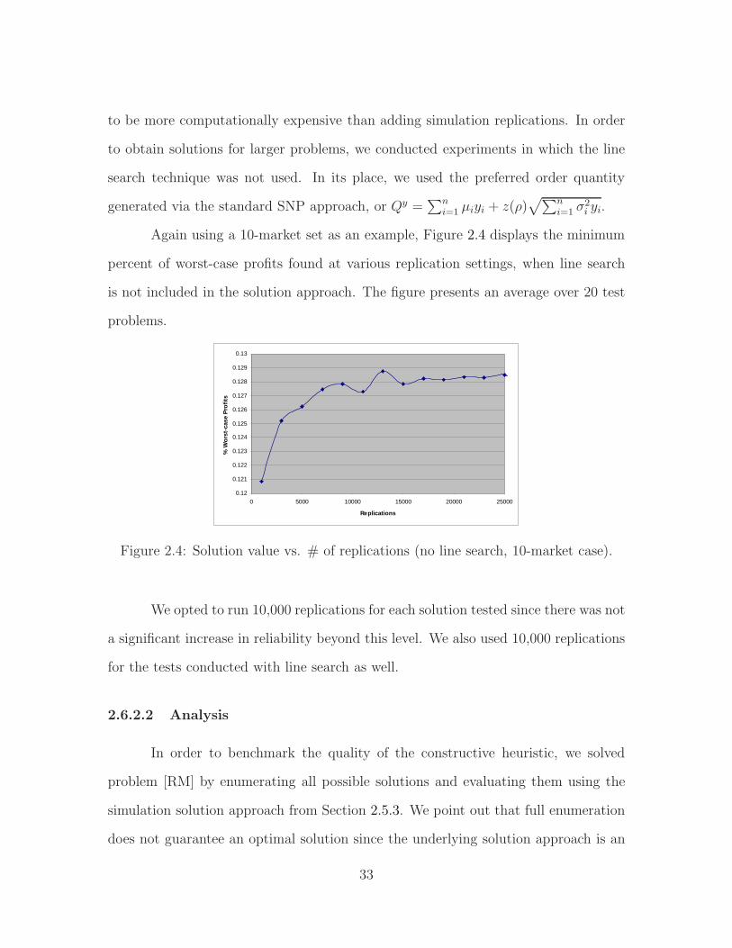
Again using a 10-market set as an example, Figure 2.4 displays the minimum

percent of worst-case profits found at various replication settings, when line search

is not included in the solution approach. The figure presents an average over 20 test

problems.

0.12

0.121

0.122

0.123

0.124

0.125

0.126

0.127

0.128

0.129

0.13

0 5000 10000 15000 20000 25000

Replications

% W

ors

t-ca

se P

rofi

ts

Figure 2.4: Solution value vs. # of replications (no line search, 10-market case).

We opted to run 10,000 replications for each solution tested since there was not

a significant increase in reliability beyond this level. We also used 10,000 replications

for the tests conducted with line search as well.

2.6.2.2 Analysis

In order to benchmark the quality of the constructive heuristic, we solved

problem [RM] by enumerating all possible solutions and evaluating them using the

simulation solution approach from Section 2.5.3. We point out that full enumeration

does not guarantee an optimal solution since the underlying solution approach is an

33

approximation via simulation. Moreover, for larger test instances, full enumeration

is not possible. Still, this does provide an important comparison for the smaller

problems.

Tables 2.1 and 2.2 present the critical performance measures using full enumer-

ation and the constructive heuristic, respectively. To address long run times within

each approach, we could either reduce the number of simulation replications or elimi-

nate the line search. We implemented the respective algorithms with line search (LS)

and without line search (NLS) to determine a preferred order quantity, and for the

four levels of profit previously mentioned. Also note that we record the expected profit

and order quantity for the standard SNP approach with no risk in the final column.

We simulated each potential solution 10,000 times except when noted differently.

Table 2.1: Enumeration Results for [RM]Solution Approach - Enumeration

Scenario/ P=0.25(GSNP ) P=0.1(GSNP ) P=0.05(GSNP ) P=0.01(GSNP ) SNPMeasurement LS NLS LS NLS LS NLS LS NLS Solutions5 MarketsCPU Time 1 sec <1 sec 1 sec <1 sec 1 sec <1 sec 1 sec <1 sec GSNP=19150G 17713 17713 17520 17520 17520 17212 17307 17212FG(P ) 0.3018 0.3101 0.2806 0.2883 0.2741 0.2813 0.2690 0.2761 QSNP=3013Q 3089 3177 2999 3081 3006 3021 2996 3021

10 MarketsCPU Time 71 sec 3 sec 71 sec 3 sec 70 sec 3 sec 70 sec 3 sec GSNP=61533G 60904 60787 59562 58723 58572 58723 58505 58447FG(P ) 0.1573 0.1591 0.1264 0.1274 0.1169 0.1183 0.1102 0.1118 QSNP=6824Q 6188 6220 5835 5681 5630 5681 5591 5602

15 Markets ∗∗ ∗∗ ∗∗ ∗∗CPU Time 5 min 2 min 5 min 2 min 5 min 140 sec 5 min 140 sec GSNP=100669G 96452 96345 96326 96773 93200 95855 93994 94805FG(P ) 0.1026 0.1053 0.0740 0.0817 0.0658 0.0742 0.0596 0.0687 QSNP=10025Q 9021 8942 8940 8777 8757 8583 8842 8400

20 MarketsCPU Time n/a 91 min n/a 89 min n/a 89 min n/a 78 min GSNP=151445G 146277 140566 137657 136464FG(P ) 0.0659 0.0447 0.0393 0.0353 QSNP=13844Q 12047 11124 10742 10660

** Results from 1000 replications

Solving each problem using full enumeration was very time consuming. Com-

bining the requirement of simulation and line search, the solution time for a 15-market

34

Table 2.2: Heuristic Results for [RM]Solution Approach - Heuristics

Scenario/ P=0.25(GSNP ) P=0.1(GSNP ) P=0.05(GSNP ) P=0.01(GSNP ) SNPMeasurement LS NLS LS NLS LS NLS LS NLS Solutions5 MarketsCPU Time <1 sec <1 sec <1 sec <1 sec <1 sec <1 sec <1 sec <1 sec GSNP=19150G 17713 17713 17520 17520 17520 17212 17307 17212FG(P ) 0.3017 0.3099 0.2805 0.2882 0.2740 0.2812 0.2689 0.2760 QSNP=3013Q 3089 3177 2999 3081 3006 3021 2996 3021

10 MarketsCPU Time 1 sec <1 sec 1 sec <1 sec 1 sec <1 sec 1 sec <1 sec GSNP=61533G 59663 58877 58473 58551 58645 58723 58407 58521FG(P ) 0.1591 0.1636 0.1264 0.1273 0.1169 0.1182 0.1102 0.1117 QSNP=6824Q 5987 6017 5566 5615 5656 5681 5550 5626






35

problem exceeded three hours per test problem. In order to still provide a comparison

at the 15-market level, we chose to use 1000 simulation replications. The constructive

heuristic was quite fast in comparison, producing results for the 50-market problems

within one minute.

Overall, we achieve similar quality solutions using our heuristic approach as

compared to the enumerative approach, with the noise in solution quality due to

the simulations required to develop the profit distribution. The heuristic approach

actually achieves a lower FG(P ) than the enumerative approach in several cases.

(Recall that the enumerative procedure is still a heuristic itself, since we must use

simulation to construct the profit distribution for every potential market selection

assignment.) Thus, it is important to note that we are not giving up much in the

way of solution quality for a significant reduction in solution time. We also point out

that when minimizing risk, the resulting expected profit values (G) are always less

than those generated for GSNP , since GSNP represents a risk-neutral approach.

We discuss more specific results for critical profit levels of 25 %, 10%, 5% and

1% of GSNP value. In these cases, we observe that the order quantity is consistently

below the corresponding QSNP . Based on the problem data used, in risk averse

settings, minimizing worst-case profits (or losses) results in ordering less. Another

key result is that FG(P ) for line search is consistently smaller than the “no line search”

approach. Moreover, the difference in solution quality (line search vs. no line search)

increases as additional markets are added to the problem, so the need to perform line

search becomes increasingly important for the 40- and 50-market scenarios. For the

10%, 5%, and 1% cases, the order quantity calculation without line search typically

underestimated the Q that produced minimal risk, further supporting the use of line

search in the solution method.

Again, with the exception of 50-market line search problem for 25%, for the

36

25%, 10%, 5%, and 1% cases, we also observe that FG(P ) decreases as number of

markets is increased. This is mainly due to the the shift in location of the profit

distribution. With an increase in the number of markets, the new 10% critical profit

level is much smaller in relation to the expected profit value. Thus, fewer profit

observations will occur below the new P .

2.7 Conclusions

In this chapter, we offer multiple approaches for assessing and evaluating the

risk associated with a particular solution to the selective newsvendor problem. For

the risk minimizing model, we introduced a constructive heuristic that provides high

quality solutions at a fraction of the time of an enumerative approach. With the

data sets tested, the selective newsvendor with risk orders less than the risk-neutral

selective newsvendor, especially for cases in which only the extreme worst-case profits

(or losses) are being minimized. The solution approach with line search provides

much better results than simply using the order quantity based on the expected value

approach of the selective newsvendor. Both the line search and simulation replications

require significant computing time, and these items must be considered as problem

size increases.

We point out that obtaining solutions to probabilistic risk models can be

quite cumbersome, and we offer approaches that firms dealing with risk issues can

implement. When there is no closed-form solution approach available for defining

the profit distribution (and worst-case profits), we must resort to an approach using

simulation as described in this chapter.

In future work, we would like to consider the benefit of including a local search

algorithm to improve the constructive heuristic solution. This would become increas-

37

ingly important as the number of markets is increased. It would also be worthwhile to

provide a large testbed of problems and observe how the solutions change across the

problems. We also plan to address the impact that various types of demand distri-

butions (such as all-or-nothing or Bernoulli demands, and uniform demands) would

have on the resulting solutions and solution approaches. Another area of interest

would be the multi-period market or order selection problem with risk. This is a very

rich area of research with lots of opportunity.

2.8 Appendix

The following figures depict the sensitivity of the solution frontiers to produc-

tion cost, salvage value, and expediting cost for models [MV-G] and [MV-R].

c=150.001

0

100000

200000

300000

400000

500000

600000

700000

800000

0 200000 400000 600000 800000 1000000 1200000 1400000

Total Variance

$

c=190

0

100000

200000

300000

400000

500000

600000

700000

800000

0 200000 400000 600000 800000 1000000 1200000 1400000

Total Variance

$

c=203

0

100000

200000

300000

400000

500000

600000

700000

800000

0 200000 400000 600000 800000 1000000 1200000 1400000

Total Variance

$

M V-G M V-R

Figure 2.5: Solution Frontier Sensitivity to Production Cost (c)

38

v=0

0

20000

40000

60000

80000

100000

120000

140000

160000

0 200000 400000 600000 800000 1000000 1200000 1400000

Total Variance

$

v=150

0

20000

40000

60000

80000

100000

120000

140000

160000

0 200000 400000 600000 800000 1000000 1200000 1400000

Total Variance

$

v=199.99

0

20000

40000

60000

80000

100000

120000

140000

160000

0 200000 400000 600000 800000 1000000 1200000 1400000

Total Variance

$

M V-G M V-R

Figure 2.6: Solution Frontier Sensitivity to Salvage Value (v)

e=200.1

0

50000

100000

150000

200000

250000

300000

0 200000 400000 600000 800000 1000000 1200000 1400000

Total Variance

$

e=500

0

50000

100000

150000

200000

250000

300000

0 200000 400000 600000 800000 1000000 1200000 1400000

Total Variance

$

e=800

0

50000

100000

150000

200000

250000

300000

0 200000 400000 600000 800000 1000000 1200000 1400000

Total Variance

$

M V-G M V-R

Figure 2.7: Solution Frontier Sensitivity to Expediting Cost (e)

39

Chapter 3

Alternate Demand Distributions

for the Risk-Averse SNP

3.1 Abstract

Consider a firm that operates in consecutive single selling seasons, delivering

its products across several markets with unique revenue and uncertain demands in

each market. Using a profit maximization approach based on a newsvendor-type

model, the firm may still incur several losses across consecutive periods in the short

run. Risk analysis with demand selection has been modeled where customer/market

demands follow normal distributions. Often a firm faces a set of potential unconfirmed

orders, where each order will either come in at a predefined level or it will not come

in at all. In this chapter, we consider these All-or-Nothing (AON) demands and

provide insights into their effect on expected profit and the frequency of extremely

costly procurement policies. Instead of solely identifying the market/demand set and

procurement quantity that maximizes expected profit, we use a Conditional Value-

at-Risk approach that allows a decision maker to control the number of profitable

40

but risky demands to consider in the overall procurement policy. This approach is

compared against an expected profit objective, and several managerial insights are

provided.


This is an era resulting in ever-decreasing product lives and, in some cases, an

increasing customer influence over a firm’s production decisions. In an effort to de-

liver to customer demands, producers are often at the mercy of a very unpredictable

demand stream (or order base). Our work is motivated by observations at a large

manufacturer whose sales teams attempt to secure orders for low-volume telecom-

munications infrastructure equipment. Unsecured orders are scheduled for a specific

period of time into the future, with limited knowledge about whether or not they

will actually materialize. These orders are customized, but only at a certain (rela-

tively late) point in the production process. So the manufacturer can, in fact, begin

procuring and assembling materials that are non-customized, and then customize the

product once orders come in. When the customer is the dominant supply chain player,

he can actually influence the manufacturer’s production timeline, and the manufac-

turer may allow customer orders/due dates within the procurement lead times for the

product (in the hopes of securing the contract).

Each customer has unique qualities, and some customers will invariably play

a more dominant role in the industry. Therefore, the negotiated price of the product

will be unique for each customer, and the salesforce allocation to each customer will

also be unique. When all markets or orders that materialize must be satisfied, this

problem becomes a classical newsvendor problem. For further research on various

types of newsvendor problems, see Khouja [29], Petruzzi and Dada [36], Bertsimas

41

and Thiele [7], Chen and Chuang [15], and Chung and Flynn [18].

As explained in the previous chapter, in our setting we permit demand selection

flexibility, which allows the firm to essentially choose which orders it wants to pursue

and satisfy. Recent research on various forms of demand selection has considered both

deterministic and stochastic demand models (see, e.g., Carr and Lovejoy [12], Petruzzi

and Monahan [37] and Taaffe and Geunes [51]). Specifically, Carr and Lovejoy [12]

study an inverse newsvendor problem by optimally choosing a demand distribution

from a set of feasible demand portfolios, which may include several customer classes.

Given deterministic demands, Geunes, Shen, and Romeijn [25] address ordering poli-

cies with customer selection for generalized classical EOQ models. When selecting

customers to generate a demand portfolio, Bakal, Geunes and Romeijn [5] consider

that each market/customer observes price-sensitive demands. Also, Yang, Yang and

Abdel-Malek [63] have studied a supplier selection problem, where a buyer faces an

uncertain demand and has to decide ordering quantities from a set of suppliers with

different yields and prices.

In stochastic demand settings, demand selection allows the firm to decide

whether it should pursue highly profitable, yet risky, orders over less profitable, but

possibly more stable orders. Thus, expected profit is now influenced by the size and

uncertainty of the order as well as the set of markets that the firm decides to satisfy.

Simultaneously selecting the most desirable market set and setting the appropriate

total order quantity has been commonly referred to as the “selective newsvendor”

problem (SNP) (see, e.g., Taaffe, Geunes, and Romeijn [53]).

All previously-cited research employs an objective of maximizing expected

profit or minimizing expected cost. However, all firms do not enjoy risk-neutral

operating conditions. In fact, many firms operate on limited operating budgets that

do not allow for incurring several losses over consecutive selling seasons. Research

42

focusing on non-risk-neutral decision makers with newsvendor operating conditions

began with Lau [31] and has grown in recent years (see, e.g., Eeckhoudt et al. [21],

Agrawal and Seshadri [2], Schweitzer and Cachon [44], Chen et al. [16], Wang and

Webster [61], and Wu et al. [62]). An introduction to the risk averse SNP is presented

in Chapter 2. We presented a risk averse model where the firm’s objective is to

minimize the number of outcomes that could occur below their targeted profit level.

In particular, we studied the effect of incorporating risk into the SNP, presenting the

analysis based on either minimizing demand uncertainty or worst-case profits. We

also demonstrated that embedding simulation into a constructive heuristic provides

high-quality market selections. This approach, as well as the risk-neutral approach

found in Taaffe, Geunes and Romeijn [53], provide solution approaches and insights

for the SNP with normally distributed demands.

In our motivating example described earlier, our firm faces a set of unconfirmed

demands or orders, and each order will either come in at a predefined level or not at

all (i.e., demands are not normally distributed). This behavior of customer demand

is modeled using a Bernoulli distribution or what we denote as all-or-nothing (AON)

demands. Taaffe and Romeijn [54] and Taaffe, Romeijn, and Tirumalasetty [55] have

addressed the AON problem with an objective of maximizing expected profit. In

this chapter, we account for the risk associated with each demand, and offer several

methods for providing the firm with more information about the relationship between

expected profit and the risk of single-period losses.

In order to incorporate risk in the AON problem, we utilize the concept of

Conditional Value-at-Risk, or CVaR. CVaR has been widely used in the field of port-

folio management, and it is rapidly gaining influence in the insurance industry as

well. Rockafellar and Uryasev [41] introduced a new approach to optimize a portfolio

in order to reduce the risk of high losses. This approach mainly tried to optimize the

43

portfolio by calculating Value-at-Risk (VaR) and optimizing CVaR simultaneously.

This approach is of particular interest to our work as the technique applied here

can be combined with analytical or scenario-based methods. Given that our prob-

lem has unique demand realization points (i.e., all-or-nothing) and, thus, has a finite

number of outcomes or scenarios, CVaR allows the evaluation of worst-case profits

and shaping of the resulting profit distribution through careful demand selection and

procurement decisions.

In summary, this chapter is an extension of both risk-averse and AON problems

in single-period settings. Past work in Chapter 2 has considered risk-averse producers

with normally distributed demands, and risk-neutral producers with either normally

distributed demands or all-or-nothing demands ([53],[55]), however these two char-

acteristics have not been addressed simultaneously. In this chapter, we model risk

analysis with demand selection where customer orders are AON, and we study its ef-

fect on demand selection, procurement policies, and the minimization of the potential

worst-case profits or losses.

Often, the firm may know a demand range for a customer and nothing more.

Considering equally likely observations in that range, a uniform distribution would

provide a good approximation. In this chapter we also model the risk analysis with

demand selection where customer orders follow uniform distribution and will study

its effect on minimizing the potential worst case losses using the simulation with local

search algorithm. This work addresses the impact that these various types of demand

distributions would have on both demand selection and procurement policies and the

applicability of the heuristic approach presented in the previous chapter.

The rest of the chapter is organized as follows. In Section 3.3 we review the

expected profit approach for all-or-nothing demands and discuss the form of the profit

distribution. In Section 3.4, we present the optimization model for all-or-nothing

44

demands under risk averse conditions. Section 3.4.3 discusses the various managerial

insights discovered via sensitivity analysis. In Section 3.6, we present the form of

profit distributions for AON and uniform distribution by using heuristics presented

in Chapter 2. Section 3.7 provides our conclusions and directions for future work.

3.3 Expected Profit Approach: AON Demands

The SNP with All-or-nothing (SNP-AON) demands has been previously stud-

ied in Taaffe and Romeijn [54] and Taaffe, Romeijn, and Tirumalasetty [55]. We

consider a set of n potential orders that a supplier can serve. Let Di denote the

random variable for demand source i (i = 1, . . . , n) with probability distribution Fi,

and assume that these demands are statistically independent. Most prior models

with selection flexibility assumed that each random variable for demand is normally

distributed. We consider that a firm may face a set of unconfirmed orders, and each

order will either come in at a predefined level, or it will not come in at all. Let pi be

the probability of an order being realized at a pre-defined level di for market i:

Pr(Di = x) =

1 − pi if x = 0

pi if x = di.

The firm must decide far in advance of the selling season both the actual

markets it will serve and the total quantity Q to be procured. We define the various

parameters as follows: let c denote a per-unit procurement cost, ri denote the revenue

associated with market i, Si denote the fixed cost for entering market i, v denote the

salvage value and e denote the shortage cost or expediting cost. Without loss of

generality we assume that ri > c, otherwise we could immediately eliminate market i

from consideration and also e > c and c > v. Let yi(i = 1, . . . , n) represent the binary

45

demand selection variables representing the firms choice to select or reject order i.

We present the following expression for the total realized profit, based on a

function G(Q, y) of the order quantity Q, the binary vector y, and the random variable

for demand Di:

G(Q, y) =

n∑i=1


i=1

Diyi) Q >∑n

i=1 Diyi

n∑i=1


i=1


, (3.1)

where∑n

i=1 Diyi represents the total demand from the selected markets. Since

E(∑n

i=1 Di) =∑n

i=1 dipi, we can then express the firm’s expected profit as:

H(Q, y) =n∑

i=1

(ridipi − Si)yi − cQ + vE

[max

(0, Q−

n∑i=1

Diyi

)]

− eE

[max

(0,

n∑i=1

Diyi − Q

)]. (3.2)

The formulation for the selective newsvendor problem for AON demands is now given

by:

maximize H(Q, y)

subject to: Q ≥ 0

yi ∈ {0, 1} i = 1, . . . , n.

A more explicit formulation of the profit function can be written by describing

the unique demand scenarios, where each scenario w is comprised of a set Iw ⊆{1, . . . , n} that contains the orders whose demands are realized. Let Pw denote the

46

probability that demand scenario w is realized and is obtained by:

Pw =∏i∈Iw

pi ·∏i�∈Iw

(1 − pi), w = 1, . . . , W.

Note that there are a total of W ≡ 2n potential scenarios. By introducing the

artificial variables uw representing the shortage in scenario w, we can restate the AON

optimization problem as the following mixed-integer linear programming problem:

[AON-EP]

maximize∑n

i=1 ((ri − v)dipi − Si) yi − (c − v)Q − (e − v)∑W

w=1 Pwuw

subject to: uw ≥∑i∈Iwdiyi − Q w = 1, . . . ,W,

Q ≥ 0

uw ≥ 0 w = 1, . . . ,W,

yi ∈ {0, 1} i = 1, . . . , n.

Taaffe, Romeijn, and Tirumalasetty [55] introduce an exact solution approach

(based on the L-shaped method) for solving this stochastic programming problem.

Their tailored algorithm can solve problems with three times as many selected or-

ders as a state-of-the-art commercial solver. For larger problem instances, due to

scenario explosion, an alternative heuristic solution is provided, and it was demon-

strated to work quite well. In the next section, we will discuss the optimization

approach (namely, CVaR) for incorporating risk into SNP with AON demands.

47

3.4 Conditional Value at Risk (CVaR) Models

Risk management is a crucial topic for researchers and market practition-

ers, with Value-at-Risk (VaR) established as a benchmark measure to evaluate risk

within the financial literature. It measures the maximum loss associated with a spec-

ified confidence level of outcomes. Although VaR has been extensively applied in risk

management, researchers have criticized this risk measure. Artzner, Delbaen, Eber

and Heath [3] pointed out that VaR is not a coherent measure of risk since it fails to

hold the subadditivity property. Moreover, VaR does not explain the magnitude of

the loss when the VaR limit is exceeded. Furthermore, it is difficult to optimize when

calculated using scenarios, and this has led to the use of an alternative measure – Con-

ditional Value-at-Risk (CVaR). Pflug [38] proved that CVaR is a consistent measure

of risk for its sub-additivity and convexity properties, and Uryasev [59] presented a

description of both (1) an approach for minimizing CVaR and (2) optimization prob-

lems with CVaR constraints. Additional examples of the use of CVaR can be found in

Rockafellar and Uryasev [41, 42], Tomlin and Wang [57] and Gotoh and Takano [26].

3.4.1 CVaR Formulation

In this section, we plan to incorporate risk into the AON-EP model from

Section 3.3. We apply a conditional value-at-risk (CVaR) approach for developing

an optimization model. CVaR, also known as expected shortfall, is a widely applied

concept in financial risk management to evaluate risk of the market portfolio. Figure

3.1 depicts a typical loss distribution for some set of instruments in a portfolio. One

would use CVaR to evaluate risk by focusing on the set of portfolio outcomes where

losses exceed the value-at-risk, or VaR. In the figure, CVaR at a 100α% level is the

expected return on the portfolio in the worst 100(1−α)% of the cases. CVaR can be

48

optimized using linear programming and non-smooth optimization algorithms, and

these techniques can effectively address large numbers of scenarios.

Freq

uenc

y

Loss in $CVaR

Probability

1 -

Maximum Loss VaR

Figure 3.1: Typical CVaR approach used in portfolio management.

When using CVaR to minimize worst-case losses (as is the case for portfolio

management), CVaR is always greater than or equal to VaR. CVaR is used in con-

junction with VaR and is applied for estimating the risk with non-symmetric return

distributions. Our approach will be to maximize CVaR in order to minimize the sce-

narios with losses below some targeted profit level (which will be VaR in our case).

Given that our demands are AON, the scenario-based approach of CVaR can be ap-

plied, and exact solutions (based on specific problem parameters) can be obtained.

CVaR can identify demands and a procurement quantity to maximize the worst-case

set of resulting profits (which may actually be losses) from the distribution of possi-

ble profit scenarios. Figure 3.2 depicts how CVaR would be applied to our selective

newsvendor setting in the presence of a profit distribution. The graph denotes the

critical profits below VaR, as well as the average of the worst-case profits or CVaR.

In setting up the formulation, we define ζ as a decision variable denoting the

VaR. Let α represent the significance level for the total profit distribution across all

scenarios. In other words, ζ or VaR is the targeted profit level below which we want to

49

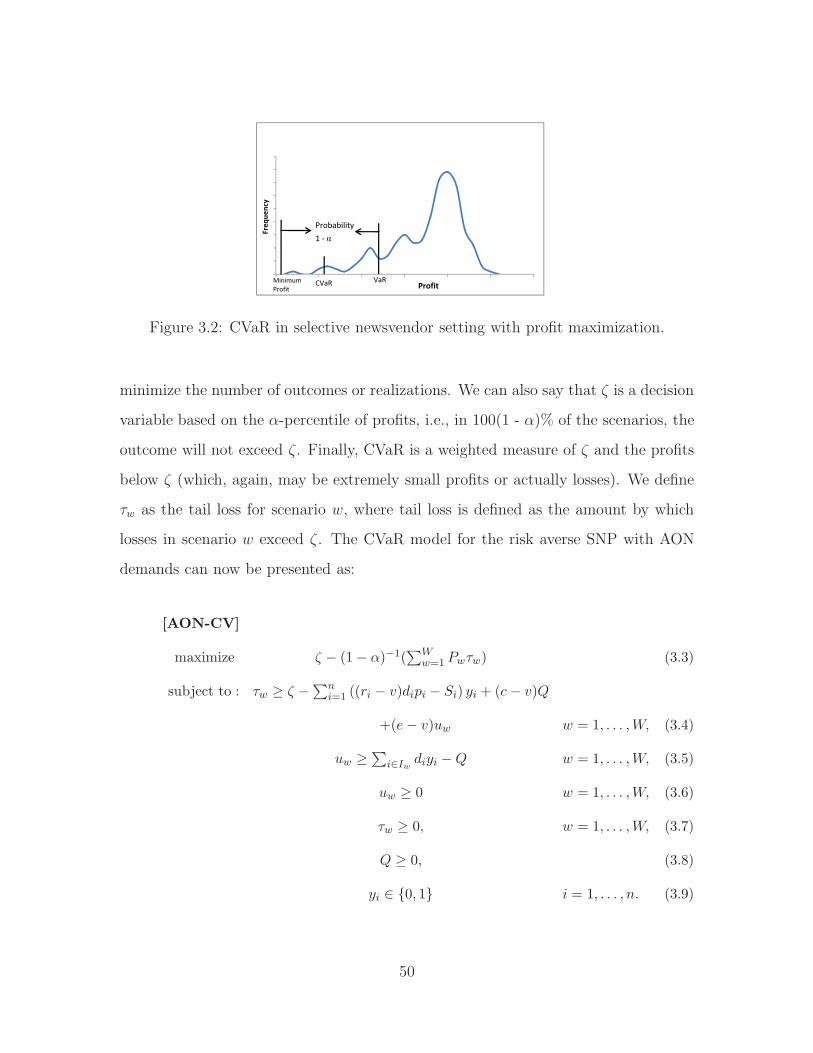
Freq

uenc

y

Profit Minimum Profit

VaRCVaR

Probability

1 -

Figure 3.2: CVaR in selective newsvendor setting with profit maximization.

minimize the number of outcomes or realizations. We can also say that ζ is a decision

variable based on the α-percentile of profits, i.e., in 100(1 - α)% of the scenarios, the

outcome will not exceed ζ . Finally, CVaR is a weighted measure of ζ and the profits

below ζ (which, again, may be extremely small profits or actually losses). We define

τw as the tail loss for scenario w, where tail loss is defined as the amount by which

losses in scenario w exceed ζ . The CVaR model for the risk averse SNP with AON

demands can now be presented as:

[AON-CV]

maximize ζ − (1 − α)−1(∑W

w=1 Pwτw) (3.3)

subject to : τw ≥ ζ −∑ni=1 ((ri − v)dipi − Si) yi + (c − v)Q

+(e − v)uw w = 1, . . . ,W, (3.4)

uw ≥∑i∈Iwdiyi − Q w = 1, . . . ,W, (3.5)

uw ≥ 0 w = 1, . . . ,W, (3.6)

τw ≥ 0, w = 1, . . . ,W, (3.7)

Q ≥ 0, (3.8)

yi ∈ {0, 1} i = 1, . . . , n. (3.9)

50

In our production setting, the manager of a risk-averse firm wants to maxi-

mize CVaR, as shown in the objective function of [AON-CV]. Note that as we have

imposed a constraint of τw being positive, the model tries to increase VaR and hence

positively impact the objective function. However, large increases in VaR will result

in more scenarios with tail losses, counterbalancing this effect. By measuring CVaR,

we consider the magnitude of the tail losses to achieve a more accurate estimate of

the risks of maximizing profit.

3.4.2 Observations and Data Analysis

In this section, we demonstrate the power of our CVaR approach in solving

the MIP formulation of the risk averse SNP with AON demands, or the AON-CV

model. All tests were conducted on a Dell desktop with a 3.0 GHz processor and

1 GB of RAM. For the implementation of our AON-CV model, we used CPLEX

10 with Concert Technology to solve mixed-integer linear problems. We considered

problem instances ranging in size from 5 to 15 potential orders. Unit revenue for the

orders were drawn independently from the uniform distribution on [275;325], denoted

by U[275;325], and the production cost and salvage values were set to be $200 and

$150, respectively. The expediting cost for the initial set of tests was set to $250.

Potential order sizes (or demands) were generated from a U[100;200] distribution,

while the associated probabilities of realization were drawn from U[0;1]. We generated

10 random problem instances for each market size. Table 3.1 summarizes the results

that compare the solutions to the expected profit and risk-averse selective newsvendor

problems with AON demands. Also note that the significance level α is set to 0.75

for the AON-CV model.

51

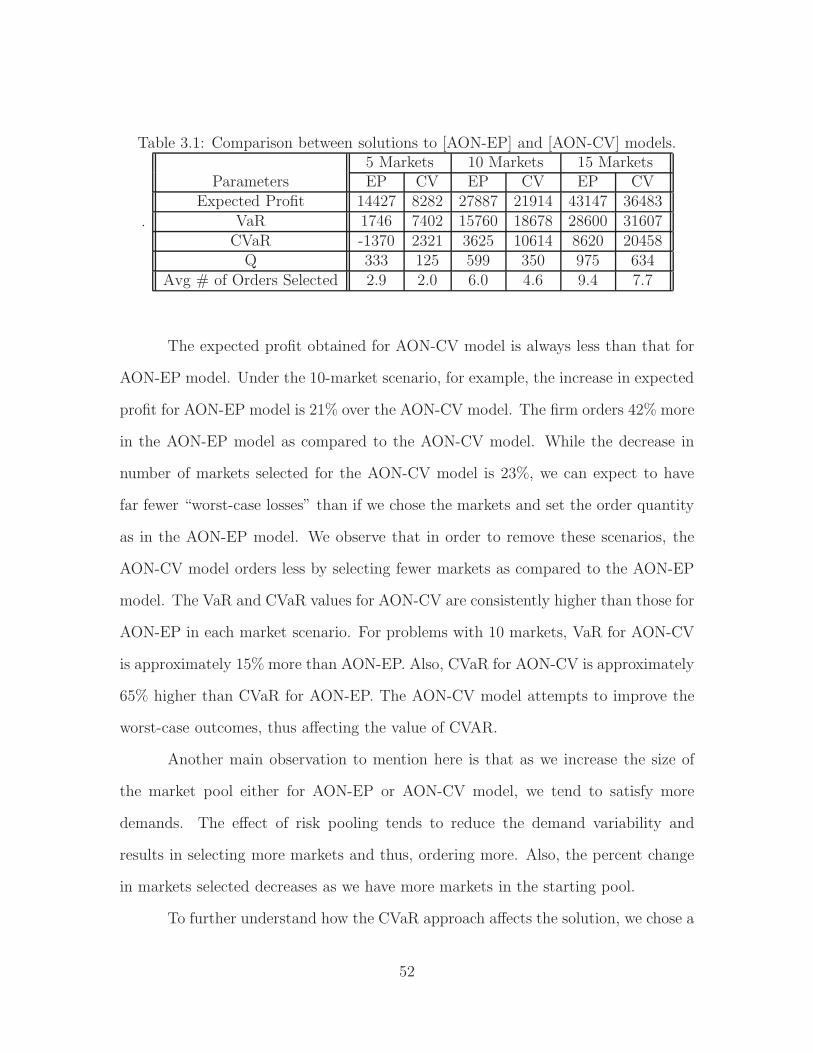
Table 3.1: Comparison between solutions to [AON-EP] and [AON-CV] models.

.

5 Markets 10 Markets 15 MarketsParameters EP CV EP CV EP CV

Expected Profit 14427 8282 27887 21914 43147 36483VaR 1746 7402 15760 18678 28600 31607

CVaR -1370 2321 3625 10614 8620 20458Q 333 125 599 350 975 634

Avg # of Orders Selected 2.9 2.0 6.0 4.6 9.4 7.7

The expected profit obtained for AON-CV model is always less than that for

AON-EP model. Under the 10-market scenario, for example, the increase in expected

profit for AON-EP model is 21% over the AON-CV model. The firm orders 42% more

in the AON-EP model as compared to the AON-CV model. While the decrease in

number of markets selected for the AON-CV model is 23%, we can expect to have

far fewer “worst-case losses” than if we chose the markets and set the order quantity

as in the AON-EP model. We observe that in order to remove these scenarios, the

AON-CV model orders less by selecting fewer markets as compared to the AON-EP

model. The VaR and CVaR values for AON-CV are consistently higher than those for

AON-EP in each market scenario. For problems with 10 markets, VaR for AON-CV

is approximately 15% more than AON-EP. Also, CVaR for AON-CV is approximately

65% higher than CVaR for AON-EP. The AON-CV model attempts to improve the

worst-case outcomes, thus affecting the value of CVAR.

Another main observation to mention here is that as we increase the size of

the market pool either for AON-EP or AON-CV model, we tend to satisfy more

demands. The effect of risk pooling tends to reduce the demand variability and

results in selecting more markets and thus, ordering more. Also, the percent change

in markets selected decreases as we have more markets in the starting pool.

To further understand how the CVaR approach affects the solution, we chose a

52

particular potential order size of 10 markets to present our observations for comparing

the AON-EP and AON-CV models. Figure 3.3 presents the differences in profit

generated from each model, at α = 0.75. GCV aR represents expected profit for [AON-

CV] and GAON represents expected profit for [AON-EP]. In addition, we indicate the

VaR and CVaR points on the AON-CV profit distribution.

0

50

100

150

-70000 -40000 -10000 20000 50000

Freq

uenc

y

Profit (in $)

AON-EP

GAONVaRCVaR

0

50

100

150

-70000 -40000 -10000 20000 50000

Freq

uenc

y

Profit (in $)

AON-CV GCVaRVaR

CVaR

Figure 3.3: AON-CV model vs AON-EP model (α = 0.75).

Notice the clustering of outcomes around the expected profit value for the

AON-CV profit distributions. We avoid extreme outcomes (both in terms of unprof-

itable outcomes and highly profitable outcomes).

It is observed that the AON-CV model has fewer worst-case profit scenarios as

compared to the AON-EP model. However, we also observed a reduction in expected

profit for the AON-CV model, which is precisely the effect of incorporating risk in

the order selection decision. Notice that the distribution becomes more peaked in the

middle, indicating a tightening of the distribution.

Taaffe et al. [55] identified specific order characteristics that are most im-

portant in the acceptance/rejection decision. While unit revenue, fixed sales costs,

demand size, and order likelihood all play a role, the results indicate that the prob-

ability that the order will materialize (or order likelihood) is the key determinant.

53

When using a CVaR objective, we are interested in observing how the set of markets

selected changes. Figure 3.4 presents an accept/reject classification of all orders for

one test instance using both the CVaR and AON-EP models, where order likelihood

is plotted against unit revenue for each order. We observe that the market selection

vector is different for the AON-EP and AON-CV models. Three markets, each with

low probability of occurrence, were initially selected in the AON-EP model are now

in the set of non-selected markets for the AON-CV model. It is interesting to know

that two non-selected markets for AON-EP model are now in set of selected markets

for the AON-CV model. Notice that in some cases orders with low unit revenue will

270280290300310320330

0 0.2 0.4 0.6 0.8 1

Uni

t Rev

enue

probability

AON-EP selected not selected

270280290300310320330

0 0.2 0.4 0.6 0.8 1

Uni

t Rev

enue

probability

AON-CV selected not selected

Figure 3.4: Orders selected: [AON-CV] vs. [AON-EP].

still be selected if the order likelihood is high.

3.4.3 Sensitivity Analysis and Insights

The AON-CV model produces an optimal solution to the the risk averse SNP

with AON demands. In this section, we provide insights and observations to assist a

decision maker in determining how certain problem parameters influence the outcomes

for expected profit, total markets selected and total order quantity in the procurement

policy. We investigate the effect of each of the following:

• Varying the significance level, α

54

• Varying the expediting cost, e

• Varying the salvage value, v

• Varying the material cost, c

In the first test, the significance level α is set at four levels of 0.5, 0.75, and

0.85, and 0.95, where the implication is that we focus on maximizing the smallest

50%, 25%, 15%, or 5% of all scenario outcomes. For the second scenario, to learn

the effects of varying expediting cost we set e at 250, 375 and 500. We then vary

the material cost and salvage cost respectively at four different settings to learn more

about sensitivity of expected profit due to changes in these costs.

3.4.3.1 Effect of Varying Significance Level α

In this section we provide our insights into the effect of varying the significance

level, α. By increasing α, we are placing additional weight on the average of the profit

outcomes below ζ , and less weight on the actual value of ζ . This has the effect of

increasing our risk aversity, since we are increasing our focus on worst-case outcomes

(or those below ζ). We selected four levels for this parameter: 0.50, 0.75 and 0.85,

and 0.95. Table 3.2 presents the comparison results for several parameters at each

significance level (when the number of markets is ten).

As we increase the value of α, the model restricts the number of outcomes

that exist below VaR. We also note that the number of selected markets decreases

quite slowly with associated increases to α. In fact, it is not until we increase from

α = 0.85 to α = 0.95 that we see a significant reduction in markets selected. We also

observed that VaR becomes greater than expected profit when α = 0.5. Similarly,

FG(ζ) = 0.414 indicates that over 40% of the profit outcomes are below ζ in this

case. With increases to α, we essentially focus on a smaller set of outcomes, and we

55

Table 3.2: Effect of varying α10 Markets, e = 250α = 0.5 α = 0.75 α = 0.85 α = 0.95

Expected Profit 25562 21914 18840 10829VaR 28068 18678 13117 5527

CVaR 17255 10615 7072 2437Q 445 350 276 129

# of Markets Selected 5.0 4.6 3.9 2.0FG(ζ) 0.414 0.197 0.094 0.021

increase the likelihood of having worst-case profits closer to VaR. Of course, this is

at the expense of expected profit.

In Figure 3.5, we plot the results of one particular instance at all significance

levels for a 10-market test instance. This setting would help us in better understand-

ing the effect of α on the AON-CV model.

Notice how there is a tightening of the profit outcomes with higher values of

α. As the decision maker becomes more risk-averse and is most concerned about only

extremely poor outcomes, all effort is placed on maximizing profit in these worst-case

scenarios. Thus, the left-hand tail of the profit distribution will be maximized at the

cost of reducing expected profit. Also worth mentioning is that there is significant

variation in the profit outcomes that define each distribution, and it is not clear how

operating at one value of α is not necessarily better than operating at another value

of α. Such a presentation of information, however, will allow a manager to make a

more informed demand management decision.

3.4.3.2 Effect of Varying Expediting Cost, e

To study the effect of expediting cost in the AON-CV model, we employed

three different levels for expediting costs as $250, $375 and $500. Using the same

56

0

50

100

150

200

-85000 -15000 55000

Freq

uenc

y

Profit (in $)

= 0.5

0

50

100

150

200

-85000 -15000 55000

Freq

uenc

y

Profit (in $)

= 0.75

0

50

100

150

200

-85000 -15000 55000

Freq

uenc

y

Profit (in $)

= 0.85

0

50

100

150

200

-85000 -15000 55000

Freq

uenc

y

Profit (in $)

= 0.95

Figure 3.5: Effect of α.

57

10-market problems as previously described, Table 3.3 presents our findings when

α = 0.75%. As the expediting cost is increased from $250 to $500, the number of

Table 3.3: Effect of varying expediting cost10 Markets, α = 0.75

e = $250 e = $375 e = $500Expected Profit 21914 14478 12395

VaR 18678 13849 10299CVaR 10614 6733 5294

Q 350 347 271# of Markets Selected 4.6 3.2 2.0

FG(ζ) 0.197 0.187 0.130

markets to be pursued by the firm decreases and, as a result, the order quantity

decreases. In this case, the reduction in number of markets selected is fairly steady,

while expected profit drops significantly from e = 250 to e = 375, as compared to the

drop from e = 375 to e = 500.

Higher expediting costs lead the firm to be more selective in how many orders

to accept and resulted in decreased expected profit. It is clear that competing firms

may find themselves in a marketplace with varying expediting costs, and knowing how

to quantify the reduction in expected profits and associated market riskiness would

be extremely beneficial during the production planning and procurement phase. The

percent of scenarios below ζ is decreasing in e, but since VaR and CVaR are both

decision variables, and since we are not directly changing α, this change in outcomes

below ζ is more difficult to interpret.

In Section 3.4.3.1, recall that an average of 2.0 markets were selected with

e = 250 and α = 0.95 in Table 3.2. Similarly, we observe that 2.0 markets were

also selected with e = 500 and α = 0.75 in Table 3.3. However, a much higher

order quantity and expected profit (on average) are associated with this result. Since

58

α = 0.75 with this higher expediting cost, we are allowing more risk into the objective.

Thus, it is not surprising that the expected profit from this particular setting is higher

than the expected profit at α = 0.95 in Table 3.2.

3.4.3.3 Effect of Varying the Salvage Value, v

Using the same 10-market problems as previously described, we used different

settings for salvage cost as follows:

• base case level as $150 (used in all test scenarios),

• salvage cost less than base case, $100,

• salvage cost more than base case but less than material cost c, $180,

• salvage cost equal to material cost c, $200.

Table 3.4 presents our findings when α = 0.75%. As the salvage cost is increased

Table 3.4: Effect of varying salvage value10 Markets, c= 200, e = 250

v = 100 v = 150 v = 180 v = 200Expected Profit 19780 21914 24268 31674

VaR 16700 18678 20222 22767CVaR 9349 10615 11946 13443

Q 295 350 386 720# of Markets Selected 4.4 4.6 4.7 4.9

FG(ζ) 0.19 0.197 0.22 0.22

from $100 to $200, the number of markets to be pursued by the firm slowly increases,

whereas the order quantity and expected profit increase dramatically. Moreover, the

increase in order quantity and expected profit is most significant when salvage cost

is increased from v = 180 to v = 200. This is due to a special structure of the

59

newsvendor problem which lets the model to order more as both salvage cost and

material cost being equal. We also note that the percent of scenarios below ζ is

increasing in v.

3.4.3.4 Effect of Varying Material Cost, c

Using the same 10-market problems as previously described, we used different

levels for material cost as follows:

• base case level as $200 (used in all test scenarios),

• material cost equal to salvage cost v, $150,

• material cost more than base case but less than expediting cost e, $230,

• material cost equal to expediting cost e, $250.

Table 3.5 presents our findings when α = 0.75%.

Table 3.5: Effect of varying material cost10 Markets, v= 150, e = 250

c = 150 c = 200 c = 230 c = 250Expected Profit 64255 21914 8787 4369

VaR 48207 18678 7289 4767CVaR 33003 10615 3247 1434

Q 958 350 146 0# of Markets Selected 6.5 4.6 4.7 1.0

FG(ζ) 0.23 0.197 0.13 0.09

Increasing material cost resulted in decreasing expected profit, VaR, CVaR,

Q and number of markets selected. This is due to a basic fundamental result that

increasing cost results in decreased demand. If we decrease material cost to a value

equal to the salvage value, as expected there is over a 65% increase in profit. However,

60

when we increased unit cost from $200 to a value equal to expediting cost, it resulted

0 units being ordered. Essentially, there is no advantage to purchasing in advance

of realizing actual demand. Thus, all demand will be satisfied through expediting.

As the material cost is increased from $150 to $250, the number of markets to be

pursued by the firm decreases and, as a result, the order quantity decreases. In this

case, the reduction in number of markets selected is fairly steady except when we

change c from 230 to 250, while expected profit drops significantly across each change

in material cost.

We introduce Figure 3.6 to depict the change in expected profit based on

changes to c, v, or e. We observe that expected profit is most sensitive to changes in

material cost, followed by expedite cost and then salvage value.

010000200003000040000500006000070000

150 200 250

Prof

it (i

n $)

material cost (in $)

05000

100001500020000250003000035000

100 150 200

Prof

it (i

n $)

salvage cost (in $)

0

5000

10000

15000

20000

25000

250 300 350 400 450 500

Prof

it (i

n $)

expedite cost (in $)

Figure 3.6: Sensitivity of expected profit due to various costs.

61

3.5 Mean-CVaR Model Considerations

Section 3.4 provided a comparison of using a risk-based objective against a

reward-based objective. The value of risk vs. reward has been a subject of extensive

research since the early works of Markowitz [33], and it deserves treatment here as

well. While a firm would like to believe it could choose to manage its procurement

and production operation using only one of these objectives, it is often most desirable

(and realistic) to consider some (convex) combination of these conflicting objectives.

We provide several mean-CVaR models to address this concern.

3.5.1 A Weighted Objective Formulation: Expected Profit

and CVaR

A firm might have conflicting desires at one time of either maximizing profit

or reducing worst-case outcomes. For these purposes, it is worthwhile to study dif-

ferent forms of risk aversion models. If we want to reduce minimum worst-case profit

outcomes, we can use the AON-CV model. For other cases, we can employ a combi-

nation of these AON-EP and AON-CV according to the criticality of each competing

objective.

One such logical extension to the AON-CV model would be the inclusion of

total expected profit in the objective function. This formulation now maximizes both

the total expected profit, AON-EP model’s objective, and the objective of AON-CV

model. All of the constraints for the AON-CV model remain, however the objective

function will now be a convex combination of the CVaR and AON objective functions.

62

We state the problem as follows:

[WOBJ]

maximize λ[∑n

i=1 ((ri − v)dipi − Si) yi − (c − v)Q −

(e − v)∑W

w=1 Pwuw] + (1 − λ)[ζ − (1 − α)−1(∑W

w=1 Pwτw)] (3.10)

subject to : 0 ≤ λ ≤ 1, (3.11)

Constraints (3.4)-(3.9),

where λ is the weighting parameter. In order to study the behavior of this model, we

chose five different values of λ as 0, 0.25, 0.5, 0.75, and 1. We provide an illustration

of the effect of using the [WOBJ] formulation to help the decision maker in setting

the optimal policy according to the firm’s importance of profit vs. risk. Table 3.6

summarizes the results for the 10-market case with e = 250 and α = 0.75.

Table 3.6: The effect of λ on model results (e=250, α = 0.75)Expected Average

Model Profit Q # Selected VaR CVaR FG(V aR) FG(20000)

AON-CV 21914 350 4.6 18678 10614 0.221 0.271

WOBJ (λ = 0.00) 21914 350 4.6 18678 10614 0.221 0.271WOBJ (λ = 0.25) 23968 388 5.0 20166 10400 0.208 0.272WOBJ (λ = 0.50) 24996 422 5.0 21530 9751 0.239 0.273WOBJ (λ = 0.75) 27231 517 5.8 21850 5706 0.235 0.277WOBJ (λ = 0.90) 27817 572 5.9 20032 3077 0.233 0.285WOBJ (λ = 0.99) 27887 599 6.0 18139 1968 0.232 0.302WOBJ (λ = 1.00) 27887 599 6.0 15760 3625 0.249 0.302

AON-EP 27887 599 6.0 15760 3625 0.249 0.302

The weighted objective with λ = 0 is the same model as [AON-CV] and thus

we have the identical results for these cases. Similarly, [WOBJ] with λ = 1 produced

the same results as [AON-EP]. Among the objective weighting options available to the

manager, the AON-EP model provides an upper bound on the expected profit value.

63

This is explained due to no involvement of risk and the objective being purely that

of maximizing expected profit. On the other hand, the AON-CV model incorporates

the risk factor and thus acts as a lower bound on expected profit. Thus, the firm can

control the level of risk allowed into the solution by setting the value of λ appropri-

ately. We note that the effect of introducing a weighting parameter λ through the

new model [WOBJ] has comparisons to adjusting the value of α in Section 3.4.3.1,

however in that case we only consider the expected profit equation implicitly through

changes to α.

The value of FG(x) represents the probability of outcomes with worst-case

profits below x, where G() is the profit equation shown in equation (4.3). In this

table, we provide FG(V aR) as well as FG(20000). As the value of λ increases, the

value of VaR is also changing. This results in no pattern or trend in how FG(V aR)

changes. However, when we consider a fixed profit value (in this case, $20,000), we can

clearly see a pattern. With increases to λ, FG(20000) also increases. In other words,

as we move towards an expected profit objective, the percentage of more extreme

scenarios being introduced into the solution also increases.

Figure 3.7 illustrates the trend of expected profit, VaR, and CVaR as a function

of λ. It appears that we observe expected profit increasing linearly with increases in

λ. However, VaR and CVaR do not follow this pattern.

3.5.2 Minimum acceptable CVaR level

Another mean-CVaR modeling approach introduces a restriction (or constraint)

on allowable worst-case profits. We use the objective of maximizing total expected

profit, while satisfying a constraint requiring the percentile of worst-case profits to be

no less than some parameter v. In other words, we use an AON-EP objective func-

tion with the AON-CV constraints, but we also include a bound on the value of the

64

0 0.3 0.6 0.9

Prof

it ($

)

Value of

Exp Profit CVaR VaR

Figure 3.7: Expected profit and “at-risk” measures vs. λ.

AON-CV objective as a constraint in this new model. We introduce this formulation

as:

[AON-MinCV]

maximize∑n

i=1 ((ri − v)dipi − Si) yi − (c − v)Q − (e − v)∑W

w=1 Pwuw

subject to : ζ − (1 − α)−1(∑W

w=1 Pwτw) ≥ v w = 1, . . . ,W,

τw ≥ ζ −∑ni=1 ((ri − v)dipi − Si) yi

−(c − v)Q − (e − v)uw w = 1, . . . ,W,

uw ≥∑i∈Iwdiyi − Q w = 1, . . . ,W,

uw ≥ 0 w = 1, . . . ,W,

τw ≥ 0, w = 1, . . . ,W,

Q ≥ 0,

yi ∈ {0, 1} i = 1, . . . , n.

In setting the value of v, we must take care in not imposing such a strict bound that

the result is always an infeasible solution. One approach would be to solve [AON-CV]

first, and then try several values of v, none of which should exceed the observed VaR

65

from the AON-CV model. To find an appropriate lower bound value on v, one could

solve [AON-CV] with a large α. We use this approach in presenting results in Table

3.7. This table provides the sensitivity of several key parameters to the value of v, at

a value of α = 0.75.

Table 3.7: AON-MinCV Model results at several CVaR levels

.

CVaR Bound Total Expected profit VaR CVaR FG(ζ) Q yv = 3000 28435 12855 3000 0.168 544 5.1v = 6000 27473 15557 6000 0.159 498 4.8v = 9000 27166 17227 9000 0.143 463 4.2v = 12000 19120 17067 12000 0.072 296 2.0

Notice how there is little change in expected profit and percent of outcomes

below ζ for v at 3000, 6000, and 9000. This is followed by a significant reduction

in profit and the number of markets selected when v = 12000. To understand this,

consider the results presented in Table 3.1. The maximum CVaR attained in the

[AON-CV] was found to be 10614 on average. If we attempt to maximize expected

profit with a bound on CVaR that is lower than 10614 (on average for the problems

tested), the expected profit objective is not significantly affected. As we increase the

CVaR bound beyond 10614, we notice much larger shifts in the characteristics in the

solution.

3.5.3 Risk Minimization with a Profit Constraint

Firms may have specific knowledge about a target minimum profit that they

require to stay in business, remain profitable, or otherwise must meet for the current

selling season. Under such a setting, the firm could be considered a “risk minimizer”

and would focus solely on minimizing worst-case profits (potentially losses) below

some critical level. In the previous chapter we present our work on this approach to the

66

so-called risk averse selective newsvendor problem RA-SNP for normally distributed

demands. A simple constructive heuristic was proposed, using simulation, to identify

markets to accept and an associated procurement policy.

We introduce the RA-SNP model and objective for comparison purposes with

the CVaR approach in this research. The RA-SNP model is presented as follows:

[RA-SNP] minimize FG(P )

subject to: Q ≥ 0,

yi ∈ {0, 1} i = 1, . . . , n.

In this model, FG is the cumulative distribution of profit and P denotes the criti-

cal profit level, below which the firm wants to minimize the potential outcomes or

scenarios.

While both [RA-SNP] and [AON-CV] are risk-minimizing models, minimizing

FG(P ) is not synonymous with maximizing CVaR. The AON-CV model approach

does not fix the value below which the percent of outcomes is minimized. Rather, we

allow the threshold value (or VaR) to be increased or decreased in order to achieve

the maximum value for CVaR. The CVaR approach indirectly results in reducing

the number of worst-case profit scenarios, and we include FG(ζ) in Table 3.6 for

this reason. Moreover, it is an exact approach to incorporate risk. The difficulty in

applying CVaR when demands are normally distributed provided motivation for the

RA-SNP modeling approach. Figure 3.8 illustrates the difference between the two

approaches. Where CVaR represented a single point on the x-axis, we have FG(P )

representing the probability of experiencing outcomes below a critical profit threshold

of P .

67

Freq

uenc

y

Profit in $

FG(P)

P

Figure 3.8: Illustration of RA-SNP approach.

3.6 Simulation Approach for Risk Averse SNP

Using simulation we will estimate the distribution for FG(ζ) for the Bernoulli

and Uniform demand distributions. A key assumption in this body of work is that

the heuristic approach developed in Chapter 2 can also be applied here. The heuristic

was based on normal demands, so it is unclear whether this will provide robust results

for uniform and Bernoulli demands. We plan to offer insights into the behavior of

these distributions when subjected to a risk averse objective. However, the purpose of

this work was to demonstrate the shape of the resulting profit distribution as well as

to observe the change in expected profit if we restrict the percent of allowable losses

or worst-case profits below the critical/acceptable profit level P.

For the case in which demands are normally distributed, expected demand

and demand variance for each market are drawn from the uniform distribution on

[500, 1000] and [50000, 100000], denoted as U[500, 1000] and U[50000, 100000]. We

simulated 10,000 profit realizations of G(Q, y) in order to estimate the shape of

the distribution for the profit equation. Unit revenue for the orders were drawn

independently from the uniform distribution on [275; 325], denoted by U[275; 325],

68

and the production cost, expediting cost, and salvage values were set to be 200, 500,

and 150, respectively. The potential order sizes (or demands) were generated from a

U[100; 200] distribution, while the associated probabilities of realization were drawn

from U[0; 1].

3.6.1 Simulation Approach for Risk Averse SNP with AON

Demands

The heuristic adopted from previous chapter is used to minimize percent of

worst case losses, and to find the associated expected profit, and order quantity

based on the markets chosen. We offer insights into the behavior of the Bernoulli and

Uniform distributions when subjected to a risk averse objective. We have considered

the 10 test instances created for each size of market pool: 10, 20, and 30. Every market

has unit revenue in the range U[$275; $325], while unit production cost is $200. The

fixed cost for market entry are drawn from U[$2500, $7500], and salvage value is set

as $150 per unit. Finally, the expediting or shortage cost is $500 per unit. We also

tested three distinct critical profit levels to observe the effect on market selection,

FG(P ) and overall order quantity. These profit levels are calculated as 25%, 10% and

5% of the expected profit given by the SNP approach without risk, denoted as GSNP ,

refer to Taaffe and Tirumalasetty [56]. All computational tests were conducted on

Dell desktop machines with a 3.0 GHz processor and 1 GB of RAM.

To obtain the estimated SNP values of G and Q for these distributions we have

applied the same formulation of SNP presented in last chapter with the exception that

mean and variance of demand were used of the respective distributions.

We consider a situation where an order may either come in at a predefined

69

level or not at all, i.e., demand for market i is governed by a Bernoulli distribution:

Pr(Di = x) =

1 − pi if x = 0

pi if x = di.

Here pi is drawn from U[0, 1]. Parameters required for performing simula-

tion tests are described as follows: expected demand for each market is indepen-

dently drawn from U[500, 1000]. Now, to correctly represent the expected demand

for Bernoulli distribution, expected demand and demand variance for each market

are given by:

µi = pi ∗ Di

σ2 = (1 − pi) ∗ pi ∗ Di

We used market pool sizes of 10, 20 and 30 and created a set of 10 test instances

for each potential market pool. We ran several similar simulation tests for various

test instances each with 10,000 realizations and obtained the consistent result for each

test instance regarding the shape of the distribution for profit equation as shown in

Figure 3.9. This figure shows the profit distribution for Bernoulli demands for a

sample test instance. It is an estimated shape of the profit equation distribution for

the risk averse AON-SNP (i.e., with demand flexibility allowing for market selection

by the firm) and the scenario when all markets have been selected for a sample test

instance. Due to the all-or-nothing demand realizations, the resulting variance is

much higher. We can still say it is left-skewed to some extent.

The heuristic adopted in chapter 2 is used to minimize number of worst-case

profit scenarios, and to find the associated expected profit, and order quantity based

on the markets chosen. In Bernoulli distribution there is probability pi associated

70

0

100

200

300

400

500

Frequency

Profit in $

AO N Dem ands M arket-Selection All-M arkets

Figure 3.9: Profit Distribution for AON.

with each demand to materialize. Table 3.8 indicates that the effect of combination

of heuristic and [RA-SNP] is minimal. There is negligible difference between the

expected values of expected profit approach and that of risk averse SNP.

Table 3.8: Procurement policies for AON demandsParameters Bernoulli Distribution Estimated

P=0.25GAON P=0.10GAON P=0.05GAON SNP values10 Markets

G 335421 338467 321620 G = 346428FG(P ) 0.132 0.048 0.032

Q 2809 2714 2565 Q = 394420 Markets

G 671765 663370 664786 G = 679655FG(P ) 0.047 0.008 0.004

Q 5536 5289 5231 Q = 778130 Markets

G 1028426 1026289 1016237 G = 1036447FG(P ) 0.022 0.002 0.000605

Q 8363 8071 7878 Q = 11892

71

3.6.2 Simulation Approach for Risk Averse SNP with Uni-

form Demands

Here the assumption is that the market demands are independently drawn

from uniform distributions. We applied the basic properties of uniform distribution

to come up with the range for market demands. We begin by assuming that we still

have µi and σ2 for each market in the range of U[500, 1000] and U[50000, 100000]

similar to the normal distribution. With known µi and (σi)2 values, we now calculate

U[ai, bi] for each market demand:

(σi)2 = (bi − ai)

2/12 , which implies (bi − ai) =√

12σi.

Now, we can find ai and bi as follows:

ai = µi −√

12σi/2

bi = µi +√

12σi/2

We ran the same type of simulation test for 10,000 profit realizations for various

test instances for each size of market pool: 10, 20, and 30. Figure 3.10 provides the

profit distribution for uniformly distributed demands for a sample test instance. We

show the risk averse SNP with market selection flexibility versus the case when all

markets have been selected.

Each time we obtained a similar shape of the distribution for the profit equa-

tion. The profit distribution is again left-skewed. As expected we observed that when

more markets have been rejected by the heuristic, then the corresponding graph has

fewer extreme losses and fewer extreme profits. The heuristic method resulted in

different market selections as compared to AON demands in above section or normal

72

0

100

200

300

400

500

Frequency

Profit in $

Uniform Dem ands M arket-Selection All-M arkets

Figure 3.10: Profit Distribution for Uniform.

demands of previous chapter. For instance, extreme values in either tail of the normal

demands distribution are less probable as compared to extreme values of the Uniform

distribution where all values are equally likely. In Table 3.9 (Uniform distribution),

Table 3.9: Procurement policies for Uniform demands

.

Parameters Uniform Distribution Estimated

P=0.25GAON P=0.10GAON P=0.05GAON SNP values10 Markets

G 78167 77930 77153 G = 82242FG(P ) 0.127 0.089 0.081

Q 6921 6876 6927 Q = 786520 Markets

G 187592 184195 180168 G = 192121FG(P ) 0.053 0.024 0.017

Q 18286 12831 13209 Q = 1628530 Markets

G 296360 294869 285853 G = 308908FG(P ) 0.022 0.008 0.003

Q 27205 25995 18259 Q = 25022

for the specific market pool we observed less than 10% reduction in expected profit

values while minimizing the worst-case losses. Also, the difference between expected

73

profit for SNP approach and that of risk averse SNP is again minute. We observed

all these results are more for the reason how the heuristic behaves rather than the

influence of demand distribution.

3.7 Conclusions

We offer several alternate market selection and product ordering models that

vary in their inclusion of risk. We introduced an exact solution approach to incorpo-

rate risk that uses Conditional Value-at-Risk via scenario analysis. We showed that

increase in the size of market selection pool increases the expected profit. Through

understanding how market selection is affected by competing objectives of expected

profit and profit risk, we provide the decision maker in any firm with a tool set for as-

sessing how much risk the firm can take. This exchange between expected profit and

risk has been presented in several ways, via a combined objective model, alternate

values for the significance level in the CVaR model, and minimum acceptable values

for CVaR. Depending on the direction governed by any project team, the decision

maker can assess the value of profit and risk to the team, and choose how to present

the recommended market selection and procurement quantity decisions to the team.

Similar to Eeckhoudt et al [21], the optimal risk averse order quantity is less

than the amount ordered by reward based model. The risk averse model also results

in fewer worst case profit scenarios as compared to the expected value solution. We

also found that the probability of materializing an order is also a key determinant in

order acceptance/ rejection decision. In risk averse model, an order will be selected

if it likelihood is high even if it has low unit revenue. We also observed that, for risk

averse setting, higher expediting and material costs resulted in decreased expected

profit and to be more selective in how many orders to accept.

74

We have tested potential market sizes from 5 to 15. While we can analyze

these cases in quite thorough detail, there is clearly motivation for studying larger

problem sizes. However, the problem suffers from the curse of dimensionality, and

the exact solution approach proposed in the current work becomes intractable using

CPLEX and Concert Technology. We plan to consider heuristic approaches to solving

such problem sizes, determining upper bounds that can help identify the quality of

solutions produced by a heuristic.

We analyzed the simulation based heuristic developed in Chapter 2 for Bernoulli

and Uniform demands. Simulation analysis helped us to investigate the resulting

profit distributions for each of the demand distributions, which are again used in de-

termining respective procurement policies. As mentioned earlier, all the results were

more influenced by the behavior of the heuristic (presented in chapter 2) as compared

to demand distributions.

3.8 Appendix

0

50

100

150

200

250

300

350

400

450

Frequency

Profit in $

Norm al Dem ands M arket-Selection All-M arkets

Figure 3.11: Profit Distribution for Normal.

75

Chapter 4

Extensions to the Selective

Newsvendor Problem

4.1 Abstract

Consider a newsvendor problem in which unique demands can be pursued

or rejected as part of the procurement plan. This has been known as the selective

newsvendor problem (SNP). In this research, we examine several extensions to the

SNP. First, we consider the impact of incorporating market-specific expediting costs

into the demand selection and procurement decisions. Second, using a lost sales

assumption instead of an expediting assumption, we perform a similar analysis by

allocating a penalty or cost for the lost sales. We present various ideas and approaches

for each of these extensions to the SNP.

76


The changing fashion trends and technological advances results in ever de-

creasing product lives and allows very little room for improvement in efficiency of

the manufacturing processes. In an effort to stay competitive, firms constantly seek

alternative ways to improve profitability. In this chapter also, we consider a supplier

or a firm that offers a product for a single selling season. The firm can obtain unique

revenues in each demand source, and it can select demand sources it wants to pur-

sue. To maximize the expected profit, the firm must simultaneously select the most

desirable demand sources as well as determine the appropriate total order quantity

before demand is actually realized. This type of demand flexibility has been previ-

ously described and modeled by Taaffe, Geunes and Romeijn [53] and Bakal, Geunes,

and Romeijn [5]. They refer to this type of problem as the “selective newsvendor

problem” or SNP. In Taaffe et al. [53], the authors show how individual demand sizes

(and the selection of those demands) can be influenced through targeted advertising

or marketing. This is introduced for operations in which marketing resources are

either unlimited or constrained. One assumption made in their research is the re-

quirement that demand in all “selected” markets be completely fulfilled, which may

require expediting from local high-cost suppliers. This is a reasonable requirement

because if the firm does not satisfy the selected markets fully, these markets may not

want to purchase again from the firm in subsequent periods. In Bakal et al. [5], they

introduce the effect of pricing considerations on market selection. In a market-specific

expediting cost extension of the SNP, we also assume that once a supplier/firm knows

the actual materialized demand, it still must satisfy all pursued demands by expedit-

ing (the portion of demand which is in excess of the total order quantity) from local

high-cost suppliers. However, we relax this assumption in a lost sales extension of the

77

SNP. We assume that if realized demand for selected markets is more than the total

order quantity, then the remaining unsatisfied portion of the realized demand is lost

and we associate a fixed penalty with this portion of the lost sales/demand.

There is an extensive literature on stochastic inventory control and more specif-

ically, the newsvendor problem, some of which are Porteus [39], Tsay, Nahmias, and

Agarwal [58], Cachon [10], and Petruzzi and Dada [36]. The classical newsvendor

problem is to find an optimal procurement policy for a product with random de-

mand during a single selling season and it has been widely studied by researchers.

In its simplest form there is a single item with stochastic demand observed for one

period. Again, a wide number of extensions have also been studied in the literature.

Khouja [29] presents an extensive literature review on the newsvendor problem and

its various possible extensions. One of the basic extensions is studying a multi-item

newsvendor case. In this extension, every item has its own unique and indepen-

dent demand and unique revenue associated with an item. Similar to a multi-item

newsvendor problem, we have different markets each with an uncertain demand and

an unique revenue associated with it. The multi-item newsvendor problem still as-

sumes all demands are included in the cumulative demand distribution, whereas, the

idea of selecting profitable (or the most desirable set of) markets differentiates our

research from the multi-item newsvendor problem. However, we review the litera-

ture to explore the existing techniques for identifying an appropriate order quantity

in a multi-item newsvendor setting. We study the possibility of blending one such

technique with our research problem based on the set of selected markets.

Hadley and Whitin [27] study the multi-item constrained newsvendor prob-

lem and presented policies to obtain the optimal order quantity. They develop two

algorithms. The first is based on a search for Lagrangian multipliers which is suit-

able when order quantities are large, and results of this algorithm will have to be

78

rounded to integers. They present a second algorithm called marginal analysis to find

an integer solution for the case when optimal order quantities are small and rounding

may have a significant impact on expected value of profits. Silver, Pyke and Peter-

son [48] provide detailed mathematical analysis of the constrained multi-item single

period newsvendor problem and a review of many extensions related to it. Moon

and Silver [35] revisit the study by Hadley and Whitin [27] on multi-item newsvendor

problem with budget constraints and fixed ordering costs. They present dynamic

programming procedures settings in which i) demands follow a normal distribution

or ii) demands are distribution-free. They also present a simple heuristic approach

for solving these problems. Abdel-Malek, Montanari and Morales [1] consider a sim-

ilar problem with budget constraints. They present an exact solution method when

the demand probability density function for each item is assumed to be uniform, as

well as a general iterative method yielding near optimal solutions for general contin-

uous density demand functions. Erlebacher [23] also presents optimal and heuristic

solutions for solving a capacitated newsvendor problem with multiple items.

Motivated from the literature presented on a multi-item newsvendor problem

and assumptions made in Taaffe et al. [53], in this chapter we present various ex-

tensions to the selective newsvendor problem. For each extension to the SNP we

present two approaches: a rationing approach and a greedy approach. In the ra-

tioning approach we ration the total shortages or lost sales across all of the selected

markets and present an exact mathematical formulation as a mixed integer nonlinear

programming problem (MINLP). We use GAMS software to solve this MINLP. For

the greedy approach, we try to satisfy the demand of most attractive markets and

allocate the shortage to a least attractive market. We show that a reasonable MINLP

cannot be formulated and solved. Instead, we introduce simulation-based heuristics

that incorporate ideas from past work with alternatives for finding the order quan-

79

tity. First, we consider the impact of incorporating market-specific expediting costs

into the demand selection and procurement decisions. Then, using a lost sales as-

sumption instead of an expediting assumption, we perform a similar analysis using a

single lost sales cost (but, in effect, this case still has market-specific characteristics

due to unique revenues in each market). The structure of our problem illustrates

similarities to that of a multi-item newsvendor problem, and literature has provided

some insights into allocating capacity to satisfy the demand of individual items. For

a given set of selected markets, we can also treat each market as an independent

newsvendor problem and find market-specific order quantities. The cumulative sum

of all individual order quantities then provides the total order quantity for the whole

set of selected markets.

In the remaining sections we explain these ideas and approaches in detail for

each of these extensions to the SNP. The rest of this chapter is organized as follows.

For a brief review of the SNP we begin with a brief introduction to SNP in Section 4.3.

In Section 4.4 we present a discussion and the problem formulation to incorporate

the effect of a market-specific expediting cost in SNP. An assumption of lost-sales is

explained in Section 4.6. Section 4.7 concludes this chapter with our remarks and

future work directions.

4.3 Selective Newsvendor Problem

Our work in this chapter builds upon the research first introduced in Taaffe

et al. [53]. To maintain consistency with prior chapters, we define Di as the random

variable representing demand in market i, (i = 1, . . . , n). Denote c as the per-unit

cost of obtaining or procuring the product to be sold. The product can be sold in

market i at a per-unit price of ri. If realized demand is less than the quantity ordered,

80

the firm can salvage each remaining unit for a value of v. If demand exceeds the order

quantity, there is a shortage cost/expedite cost of e per unit in market i.

Let yi = 1 if the firm decides to satisfy demand in market i, and 0 if the firm

rejects market i’s demand. Also assume that Si represents the entry or fixed cost

of choosing market i. The total realized profit, based on the order quantity, market

selection decisions, and realized demand, is expressed as follows:

H(Q, y) =

n∑i=1


i=1

Diyi) Q >∑n

i=1 Diyi

n∑i=1


i=1


.

Given a binary vector of market selection variables y, and letting Dy =∑ni=1 Diyi represent the total demand of the selected markets, the mean and vari-

ance of total demand are E(Dy) =∑n

i=1 µiyi and Var(Dy) =∑n

i=1 σ2i yi, respectively.

Then the firm’s expected profit is expressed as a function G(Q, y) of the order quantity

Q and the binary vector y:

G(Q, y) =

n∑i=1

(riµi − Si)yi − cQ + vE

[max

(0, Q −

n∑i=1

Diyi

)]

− eE

[max

(0,

n∑i=1

Diyi − Q

)]. (4.1)

The general selective newsvendor problem [SNP] is now given by

[SNP] maximize G(Q, y)

subject to: Q ≥ 0 (4.2)

yi ∈ {0, 1} i = 1, . . . , n. (4.3)

As shown in Section 2.3.1 there exists an optimal solution for the case of normal

81

demands using sorting mechanism defined by DERU property.

4.4 Market-Specific Expediting Cost

We now suppose that the cost to expedite units after demand realization is

market-specific, i.e., we let ei denote the cost per unit for expediting units to market i

after demand is realized. We would like to mention that in some cases expediting costs

can exceed the revenue generated for a particular market, thus leading to reasons that

we would not select a market. However, demand uncertainty also plays a large role

in defining the attractiveness of a market. Thus, the less predictable that demand is,

the more likely it is that we will not select that market. We define different sorting

mechanisms to select markets based on various key indicators such as ei, ri, µi and σ2i .

We must now define a strategy for allocating the original Q units received from the

overseas supplier, thus determining the amount of “shortage” each selected market

faces upon demand realization. We present two allocation approaches: rationing and

greedy.

4.4.1 Rationing the Shortages

In this approach we ration shortages equally among all markets. Consider I1

to represent the set of selected markets. Then, for a given vector y, the shortage in

market i now becomes:

(Dy − Q)+

|I1| ,

82

where |I1| =∑

i∈I1yi, which is simply the number of selected markets. The expected

shortage cost for market i can then be written as

ei

|I1|

∞∫Q

(Dy − Q)f(Dy)dDy =ei

|I1|ΛDy(Q).

where we define ΛDy(Q) as the loss function for a given order quantity Q and market

selection vector y. The expected total profit equation now becomes

G(Q, y) =∑i∈I

(riµi − Si)yi − cQ + v

∫ Q

0

(Q − Dy)f(Dy)dDy −∑i∈I1

ei

|I1|ΛDy(Q). (4.4)

Given the vector y then, our optimal order quantity is determined by the

following equation:

FDy(Q∗y) =

(∑i∈I1

ei∑i∈I1

yi− c

)/

(∑i∈I1

ei∑i∈I1

yi− v

)= ρ, (4.5)

where ρ denotes the critical fractile based on the markets selected. Note that we can

actually find an optimal Q∗y assuming prior knowledge of market selection vector y,

however our focus is concerning those situations where market selection is not known.

In this case, the critical fractile is a function of the markets selected. We attempt to

make a special note here that rationing shortages would only be prudent if a particular

market would actually notice the shortage (i.e., the shortage would cause a portion of

the market’s order to arrive late). Otherwise, we should always allocate the overseas

product to the markets with the highest shortage costs first when the market is not

aware that any shortage actually occurred. Without a late arrival of product to a

market, there would appear to be no motivation for rationing shortages.

Since Dy is normally distributed, we can write the optimal order quantity as

83

Q∗y =

∑ni=1 µiyi + z(ρ)

√∑ni=1 σiyi, where z(ρ) =

Q∗y−µy

σy= Φ−1(ρ) is the standard

normal variate value associated with the fractile ρ. We can write the loss function

ΛDy(Q∗y) in terms of the standard normal loss function L(z) =

∫∞z

(u−z)φ(u)du, where

φ(u) is the p.d.f of the standard normal distribution, with c.d.f Φ(u). In particular,

ΛDy(Q∗y) = σyL(z(ρ)). We can write the expected profit equation as follows:

G(Q, y) =∑i∈I

(riµi − Si)yi − cQ − v

∫ Q

0

(Dy − Q)f(Dy)dDy −∑i∈I1

ei

|I1|ΛDy(Q)

=∑i∈I

(riµi − Si)yi − cQ − v

∫ Q

0

(Dy − Q)f(Dy)dDy

− v

∫ ∞

Q

(Dy − Q)f(Dy)dDy + v

∫ ∞

Q

(Dy − Q)f(Dy)dDy −∑i∈I1

ei

|I1|ΛDy(Q)

=∑i∈I

(riµi − Si)yi − cQ − vµiyi + vQ + vΛDy(Q) −∑i∈I1

ei

|I1|ΛDy(Q)

=∑i∈I

((ri − v)µi − Si)yi − (c − v)Q + vΛDy(Q) −∑i∈I1

ei

|I1|ΛDy(Q).

We rewrite the expected profit equation as:

G(Q, y) =∑i∈I

((ri − v)µi − Si)yi − (c − v)Q + vΛDy(Q) −∑i∈I1

ei

|I1|ΛDy(Q). (4.6)

We formulate our mixed integer programming problem for the case of rationing short-

ages as:

[R-SNP] maximize G(Q, y)

subject to: Q ≥ 0, (4.7)

yi ∈ {0, 1} i = 1, . . . , n. (4.8)

where G(Q, y) is defined by (4.6). The following paragraph describes the parameters

84

used in greater detail. We varied the size of the market pool between 5 and 50 markets,

depending on the experiments being conducted. Every market has unit revenue in the

range U[$212,$252], while the unit production cost is set at $200. Expected demand

and demand variance for each market are distributed according to U[800,1200] units

and U[30000,60000], respectively. The fixed cost for market entry are drawn from

U[$10000,$15000]. The expediting cost for each market is drawn from U[$400, $500].

Finally, the salvage value is $150 per unit. We use this same data set for all the

computational tests through out this chapter. We use GAMS software to optimally

solve [R-SNP]. We utilize Lindoglobal solver to optimally solve this MINLP problem.

Lindoglobal in GAMS reports the global optimal solution to the problem on hand. We

present the average results from ten test problems for each market pool in Table 4.1.

Table 4.1: Base case: Rationing the ShortagesMarkets Expected Profit Order Quantity Markets Selected fractile

5 64525 4908 4.5 0.8510 137735 9974 9.3 0.8515 215756 14407 14 0.8520 300071 19010 18 0.8630 479812 28782 28 0.8540 634630 38627 37 0.8550 834311 48390 47 0.85

We observe that as the number of markets under consideration for selection

increases, risk pooling allows the selection of more markets and hence allows for or-

dering more, resulting in an increase in average profit. The critical fractile remains

nearly constant over all market sets. This is intuitive as we can control the markets

selected and order quantity, while the input cost and revenue parameters remain un-

changed. To provide various managerial insights, we perform the sensitivity analysis

85

by varying the different cost parameters and study their impact on the structure of

the SNP. For the 10-market problem setting, the unit cost c is varied at three levels:

$170 which is near the salvage cost of $150, $188 which is below base unit cost of

$200 and $212 which is higher than base unit cost and near to per unit revenue. Sim-

ilarly, expediting cost is then varied at three levels: U[$250,$350], U[$350,$450] and

U[$450,$550]. We conclude by studying the impact of varying per unit revenue on the

procurement policies. We start the range of per unit revenue equal to the unit cost

U[$200,$240], slightly greater than unit cost U[$202,$242] and a larger increase over

unit cost U[$225,$265], which is also higher than the base case. Table 4.2 summarizes

all the results.

Table 4.2: Varying the parameters: Rationing the shortagesParameters Level 1 Level 2 Level 3Unit Cost c=$170 c=$188 c=$21210 Markets

Expected Profit 461253 264920 44914Order Quantity 11037 10797 6175Markets Selected 10 10 5.7

ρ 0.93 0.87 0.90Expediting Cost ei=U[$250,$350] ei=U[$350,$450] ei=U[$450,$550]

10 MarketsExpected Profit 151456 141044 135088Order Quantity 9704 9983 10040Markets Selected 9.4 9.4 9.4

ρ 0.69 0.81 0.87Revenue ri=U[$200,$240] ri=U[$202,$242] ri=U[$225,$265]

10 MarketsExpected Profit 50246 62450 266620Order Quantity 6342 6778 10679Markets Selected 5.8 6.2 10

ρ 0.92 0.83 0.91

We observe that if the unit cost gets closer to the salvage cost, the model tends

to order more and has the highest expected profit. The expected profit decreases as

86

we move c = $170 to c = $212. When the unit cost is set equal to the lower end

of the range for the per unit revenue, the model tends to order less due to fewer

profitable markets. This tends to decrease the number of selected markets and hence

the expected profit. When the lower end of the expediting cost is changed from $250

to $450 the decrease in expected profit is about 10%. By changing the revenue’s lower

end from $200 to $202, there is around 6% increase in the order quantity resulting

in 20% increase in the expected profit. Again, by increasing the revenue from $212

to $225, the expected profit almost gets doubled. We also observed that ρ is also

changing for each parameter variation. ρ is calculated using expediting cost and

material cost. Thus changes in these also result in change in value of ρ . However,

change in ρ is not directly explained by change in values of revenue. As ρ is the point in

the demand distribution (ordering decision) corresponding to the maximum expected

profit. Also increase in revenue results in ordering more amount which indirectly

incorporates the corresponding adjustments in ρ. From this sensitivity analysis we

infer that the expected profit obtained by this model is comparatively more sensitive

to the changes in the unit material cost and the per unit revenue as compared to the

expediting or salvage cost.

4.4.2 Greedy Approach

In the greedy approach, we allocate a shortage to the least attractive market in

a set of selected markets. The market attractiveness is defined by the expediting cost

associated with each market. Suppose that if total demand from all markets selected

exceeds Q we then allocate the Q units in decreasing order of market shortage cost,

i.e., to the highest shortage cost market first. By re-sorting markets in decreasing

order of shortage cost, we have the following analysis. Clearly, we only incur a

87

shortage cost for market 1 if Q < D1, and in this case, the amount of the shortage

equals D1 − Q; similarly, we incur some shortage cost in market 2 if Q < D1 + D2,

and in this case the amount of the shortage equals D2 if D1 > Q, and D2 + D1 − Q

otherwise. In general, given that∑i

j=1 Dj > Q, the amount short in market i equals

Di if∑i−1

j=1 Dj > Q and∑i

j=1 Dj − Q otherwise.

To streamline our notation, let D[i] =∑i

j=1 Dj , and let f[i](D[i]) and F[i](D[i])

denote the pdf and cdf of D[i]. The shortage cost for market i equals

ei

{Di × Pr[D[i−1] ≥ Q] + (D[i] − Q)+Pr[(D[i−1] ≤ Q)]

}= eiDi(1 − F[i−1](Q)) + ei(D[i] − Q)+F[i−1](Q).

The expected shortage cost for market i, which we denote by Γ(i), therefore

equals

Γ(i) = eiµi(1 − F[i−1](Q)) + eiF[i−1](Q)

∫ ∞

Q

(D[i] − Q)f[i](D[i])dD[i].

For a given selection of markets (which we denote by y), our expected profit equation

(4.1) now becomes

G(Q, y) =∑i∈I

(riµi − Si)yi − cQ + v

∫ Q

0

(Q − Dy)f(Dy)dDy −∑i∈I

Γ(i), (4.9)

The problem here appears to be that we must know what markets we select

to even compute the Γ(i) values, and our critical fractile value will be a function of

our market selection decisions. Since the Γ(i) values and the critical fractile value are

functions of our market selection decisions, we cannot arrive at a formulation that

removes the selection variables from consideration (as is the case in [SNP-N]). We

may draw some conclusions based on the conditions for which (4.9) is concave, and

88

this may shed some light on any special conditions in which this may be true. We

first proceed with the partial derivative of Γ(i) with respect to Q. We show both the

first and second partial derivatives.

∂Γ(i)

∂Q= eif[i−1](Q)

[∫ ∞

Q

(D[i] − Q)f[i](D[i])dD[i] − µi

]+ eiF[i−1](Q)

[F[i](Q) − 1

]∂2Γ(i)

∂Q2= 2eif[i−1](Q)

[F[i](Q) − 1

]+ eiF[i−1](Q)

[f[i](Q)

]

Now, taking the second derivative of the entire expected profit equation (4.9)

results in:

∂2G(Q, y)

∂Q2= vfDy(Q)︸︷︷︸

≥0

−∑i∈I

ei

2f[i−1](Q)

[F[i](Q) − 1

]︸︷︷︸≤0

+ F[i−1](Q)f[i](Q)︸︷︷︸≥0

This has not led to identifying any conditions for concavity. Let’s consider

only a 2-market scenario. Then, the test for concavity is determined by

∂2G(Q,y)∂Q2 = vfDy(Q) − e1

(2f[0](Q)

[F[1](Q) − 1

]+ F[0](Q)f[1](Q)

)−e2

(2f[1](Q)

[F[2](Q) − 1

]+ F[1](Q)f[2](Q)

)= vfDy(Q) − e2

(2f[1](Q)

[F[2](Q) − 1

]+ F[1](Q)f[2](Q)

)

And, again, identifying conditions when ∂2G(Q,y)∂Q2 < 0 will be difficult to deter-

mine. One potential approach is to develop a heuristic to assess market attractiveness

based on ei, ri, µi, and σ2i . Using a heuristic we enumerate the “high quality” permu-

tations, and find the preferred selection and procurement decisions for each ordering.

This heuristic is explained in detail in the following section.

89

4.5 Construction of Heuristic

We developed a heuristic approach to obtain the procurement plans for the

market-specific expediting cost generalization to the SNP. To find both the preferred

market selections as well as an associated order quantity; we propose an approach that

examines solutions resulting from each of several market rankings. We use a similar

approach to the DERU described in chapter 2, in that we add one market at a time

and compare against the incumbent (or best-known) solution. We summarize the

main steps necessary in developing the heuristic and solving this problem as below:

I Sort the markets. To begin with we need to find the set of selected markets (y).

We develop various sorting schemes to define the attractiveness of a market.

II Determine the order quantity. For this given set of selected markets y, we now

determine the order quantity Q.

III Select markets and create a secondary sort for allocating shortages. Once we

know Q, the next decision is to allocate this order quantity among the selected

markets to obtain maximum expected profit. After the markets have been

sorted, to allocate the total order quantity as explained in Section 4.4.2,we now

sort the markets based on non-increasing expedite cost, but this time we only

sort markets that are part of the current selection vector.

IV Simulation: Repeat the process for many demand realizations. Repeat the

whole process for many demand realizations. Find the maximum average profit

over all the simulation replications.

I. Sort the Markets. We use various sorting schemes to rank markets and obtain

solutions that maximize expected profit where expected profit is reported as the

average of thousands of simulation outcomes. We list the tested rankings below:

90

1 Non-increasing expedite cost, [EC]. We sort the markets based on non-increasing

values of expedite cost. In this way we give preference to the most expensive

markets in terms of expediting cost.

2 DERU ratio. Index markets in decreasing order of expected net revenue to

uncertainty (demand variance).This ratio ordering is intuitive, as a higher net

revenue makes a market more attractive, while increases in the market’s uncer-

tainty lead to a less attractive market. DERU is shown to be optimal for SNP

in (cf. Taaffe et al. [53]).

3 Non-increasing expected net revenue, [REV]. Rank markets in non-increasing

order of their expected net revenue. This way we give first preference to the

most lucrative markets followed by less profitable ones.

4 Non-decreasing uncertainty (or demand variance), [VAR]. Sort the markets

based on increasing variance in demand. Market with least demand variance

is first in sorted array and is given the first preference to be selected in the

solution vector. This way we try to first satisfy more stable markets/customers

over highly risky ones.

5 DERU and expediting cost, [DERU*EC]. i.e. Non-increasing order of expected

net revenue to the product of expedite cost & demand variance. This ratio is the

combination of the first two sorting schemes providing with the most attractive

and more stable market at the top of rankings.

II. Determine Order Quantity. Once sorting mechanism is complete, the next

step is to determine the total order quantity. We adopt the following various options

to find the total order quantity.

91

A We consider each market as an independent single item newsvendor problem.

In an one period single item newsvendor setting an optimal order quantity is

Q∗ = F−1(ρ), where ρ = e−ce−v

. Here we find ρi = ei−cei−v

and subsequently find Qi

for each market. We then add Qi’s only for the selected markets.

B For each potential market selection find Q based on the rationing approach, i.e.,

blending the expediting costs of the selected markets and then calculating the

critical fractile ρ.

C Use the above option (option B), but place more weight on those markets with

lower expediting costs, as these would be the ones where shortages would possi-

bly occur. We multiply the expediting cost of the sorted market with the rank

of the market in a sorted array. If Wi be the rank of the market i in the sorted

market selection vector, then we represent the critical fractile ρ as follows:

FDy(Q∗y) =

(∑i∈I1

Wi ∗ ei∑i∈I1

Wi ∗ yi− c

)/

(∑i∈I1

Wi ∗ ei∑i∈I1

Wi ∗ yi− v

)= ρ, (4.10)

III. Select Markets, Sort and Allocate. Next step is to allocate the total order

quantity in order to maximize the average profit for a firm. If the total demand from

all markets selected exceeds Q we then allocate the Q units in decreasing order of

market shortage cost, i.e., to the highest shortage cost market first.

IV. Repeat For Many Demand Realizations. We save a solution for each

ranking, where solution k of a given ranking will contain all markets 1...k of that

ranking. This solution approach does not require evaluating all 2n possible market

selections, which would be computationally prohibitive. While we may miss certain

solutions, testing five unique rankings alleviates this problem to some extent.

The implementation of the heuristic is described as follows:

92

1 Generate the realized demand for each market and store these realized (or sim-

ulated) demands for all simulation runs.

2 As yi is a binary variable, we put zero for all i in initial market selection vector.

3 Sort markets based on one of five above mentioned ranking mechanisms.

4 Find the total order quantity using any one of three previously mentioned op-

tions for the given market selection.

5 For each simulation run, add markets one by one to the selection vector, calcu-

lating realized profit after each market addition. When a shortage occurs:

• Greedy approach: distribute available product to markets with highest

expediting cost markets first.

• Rationing approach: distribute available product equally across chosen

markets.

6 Tabulate realized profits for all market selection vectors across all simulation

runs.

7 Calculate the average profit for each ranking, and select the market selection

vector with the highest average profit across all simulation runs. We added the

corresponding order quantity for this solution.

4.5.1 Rationing Approach

We used the heuristic as mentioned in Section 4.5 to test a rationing approach

for several market selection alternatives. We evaluate all of the previously mentioned

ranking schemes. The only difference here is that we find the order quantity, Q, using

93

the critical fractile as given by the option B. We tested the quality of solutions ob-

tained from the heuristic against the solutions by the exact optimization formulation

using GAMS. For one particular test instance for 5 and 10 markets, we obtain solu-

tions from the heuristic for all five rankings and compare it against the corresponding

solutions by solving MINLP using GAMS. For the purpose of studying the impact of

the randomness due to the simulation based heuristic approach, we test the heuristic

for 10,000, 100,000 and 1,000,000 replications. We tabulate our observations in the

Table 4.3. We notice that the heuristic provided approximately similar quality re-

sults as by GAMS for 100,000 replications. However, running 100,000 replications is

computationally prohibitive, thus leading us to use 10,000 replications to reduce the

complexity of the heuristic to obtain the good quality procurement policies even for

big market size problems.


We employ simulation to generate demand realizations of all markets, in order

to generate the average profit across all simulations (or demand scenarios). Using the

same data as previously explained in the rationing approach, we run 10,000 simulation

replications and 100 test instances for every market pool size and report the average

values for each ranking. we employ this heuristic using all three options to determine

the order quantity. Table 4.4 summarizes results for the heuristic employing option

A to find the order quantity for the selected markets. After finding procurement

policies based on these rankings, we provide the best and worst rankings in terms

of average profit. In this table, we observe that the ranking based on combination

of DERU and expediting cost performs best for five out of seven market selections.

As this ranking tries to first satisfy the demand of the market with highest revenue,

94

Table 4.3: Comparison: Heuristic vs GAMSParamters [EC] [DERU] [VAR] [NR] [DERU ∗ EC] GAMS5 Markets Solution - Heuristic-10,000 replications

Average Profit 88386 89386 88469 89386 89386 89474Q 3874 4557 5492 4557 4557 4557

Markets Selected 3.0 4.0 5.0 4.0 4.0 4.05 Markets Solution - Heuristic-100,000 replications

Average Profit 88119 89304 88235 89304 89304 89474Q 3874 4557 5492 4557 4557 4557

Markets Selected 3.0 4.0 5.0 4.0 4.0 4.05 Markets Solution - Heuristic-1,000,000 replications

Average Profit 88119 89304 88235 89304 89304 89474Q 3874 4557 5492 4557 4557 4557


Average Profit 72668 72926 72668 72926 72926 72551Q 5000 4061 5000 4061 4061 4061


Average Profit 72443 72537 72443 72537 72537 72551Q 5000 4061 5000 4061 4061 4061

Markets Selected 5.0 4.0 5.0 4.0 4.0 4.05 Markets Solution - Heuristic-1,000,000 replications

Average Profit 72443 72537 72443 72537 72537 72551Q 5000 4061 5000 4061 4061 4061

Markets Selected 5.0 4.0 5.0 4.0 4.0 4.0

95

highest expediting cost and most stable market in terms of demand variance. Hence

resulting in the highest average profit from the selected set of markets. However, the

ranking using expected net revenue also provided approximately as good results as

the best ranking, because this ranking allocates the shortages to the least profitable

market in terms of the expected net revenue. DERU ranking performed little less

than these two rankings. Whereas, the ranking based on demand variance performed

worst among all rankings. This ranking mainly focuses on allocating shortages to

most unstable market with least expediting cost while ignoring the associated revenue

parameter. The best ranking result always outperformed worst result by 100% gain

in average profit except for the case of 50 markets, where the gain is around 90%.

Table 4.5 provides average results by the heuristic using option B to find the order

quantity for the markets in the selection set y. In this heuristic, the ranking based

on expected net revenue and the combination of DERU and expediting cost ranking

provided the best results. However, all the rankings performed almost equally good

except for the 5 market scenario. Here, the ranking based on demand variance again

provided worse results. Average profit, the total order quantity and the number of

markets selected increases with the increase in the size of the market explained by

the risk pooling factor. Table 4.6 tabulates all the results from the heuristic using

option C to find the total order quantity for y. Similar to the previous heuristic,

this one also provides approximately similar results for all five rankings except for 5

market scenario. This heuristic however performed slightly better than the heuristic

using option B for determining the order quantity for the selected markets. Whereas,

the heuristic using option A ( treating each market as an independent newsvendor

problem) performed best in 20% cases among three heuristics. Whereas, the heuristic

based on option C performed best for the rest 80% of the cases. The reason might be

the way Q has been calculated by assigning higher weights to low expediting costs.

96

Table 4.4: Greedy approach for the ei case using option A for QParamters Expedite Cost DERU Ratio Net Revenue Uncertainty [DERU*EC]5 Markets

Average Profit 44956 73671 88383 44317 91792Q 5385 3892 4407 5833 4248

Markets Selected 4.5 3.2 3.7 4.8 3.510 Markets

Average Profit 90462 152880 187278 86255 183926Q 11335 8171 8599 11908 8782


Average Profit 142568 263007 296125 140908 262165Q 17332 12131 12615 17911 13084


Average Profit 186559 352268 366061 178545 395411Q 23302 15894 16030 23642 15817


Average Profit 276748 541356 553961 276119 560512Q 35364 23570 23945 35833 25062


Average Profit 368356 655366 693595 364600 734242Q 47407 32121 32648 48246 32912

Markets Selected 39.2 26.4 26.9 40 27.150 Markets

Average Profit 453309 808921 814139 459181 874506Q 59507 40364 40495 60287 41256

Markets Selected 49.3 33.2 33.3 50 33.9

97

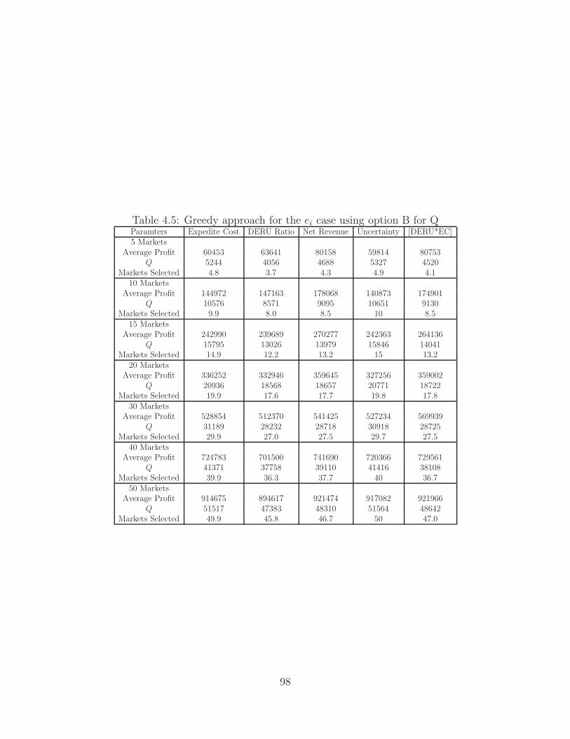
Table 4.5: Greedy approach for the ei case using option B for QParamters Expedite Cost DERU Ratio Net Revenue Uncertainty [DERU*EC]5 Markets

Average Profit 60453 63641 80158 59814 80753Q 5244 4056 4688 5327 4520


Average Profit 144972 147163 178068 140873 174901Q 10576 8571 9095 10651 9130


Average Profit 242990 239689 270277 242363 264136Q 15795 13026 13979 15846 14041


Average Profit 336252 332946 359645 327256 359002Q 20936 18568 18657 20771 18722


Average Profit 528854 512370 541425 527234 569939Q 31189 28232 28718 30918 28725


Average Profit 724783 701500 741690 720366 729561Q 41371 37758 39110 41416 38108


Average Profit 914675 894617 921474 917082 921966Q 51517 47383 48310 51564 48642


98

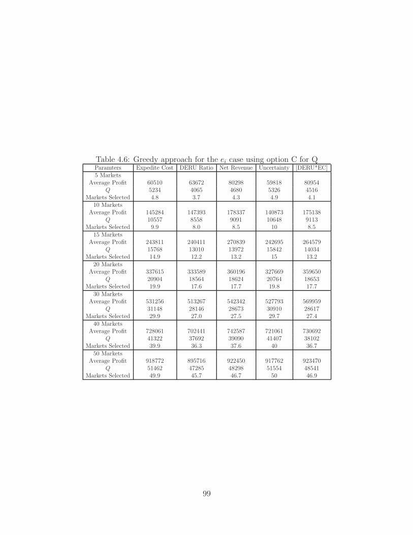
Table 4.6: Greedy approach for the ei case using option C for QParamters Expedite Cost DERU Ratio Net Revenue Uncertainty [DERU*EC]5 Markets

Average Profit 60510 63672 80298 59818 80954Q 5234 4065 4680 5326 4516


Average Profit 145284 147393 178337 140873 175138Q 10557 8558 9091 10648 9113


Average Profit 243811 240411 270839 242695 264579Q 15768 13010 13972 15842 14034


Average Profit 337615 333589 360196 327669 359650Q 20904 18564 18624 20764 18653


Average Profit 531256 513267 542342 527793 569959Q 31148 28146 28673 30910 28617


Average Profit 728061 702441 742587 721061 730692Q 41322 37692 39090 41407 38102


Average Profit 918772 895716 922450 917762 923470Q 51462 47285 48298 51554 48541


99

4.6 Lost Sales Case

Under the case of lost sales, we assume that any realized market demand not

satisfied through the procurement quantity will be lost. Assume the cost per unit

of a lost sale is l, the same across all markets, and that the individual markets will

not know if their requests will be satisfied until all demand has been realized. The

question is, can we set a policy and determine mathematically the optimal procure-

ment quantity Q∗ and market selection vector y such that we maximize our expected

profit?

There are actually two decisions to make. First, how much product should

we purchase from the overseas supplier? Then, once the individual market demand

is realized, how should we allocate our supply? Let’s assume that the procurement

quantity from the supplier has been set. Since our assumption is that the per-unit lost

sale cost is identical for each market, then the only discriminating factor across all

markets is the market-specific revenue of ri per unit. Therefore, an optimal allocation

strategy would simply be to arrange the markets in non-increasing order of per-

unit revenue and allocate the supply until it has been consumed. This assumes, as

stated earlier, that we do not need to commit to any market orders prior to demand

realization. For the sake of the following discussion, we will place all markets in

non-increasing order of per-unit revenue.

To determine the appropriate expected profit equation under the lost sales

case, we include the salvage amount based on excess supply purchased, the lost sale

amount based on the demand not satisfied, the total material or purchase cost for the

procurement quantity, and the revenue achieved through our allocation policy. We

100

state this expected profit equation as

G(Q, y) = −cQ + v

∫ Q

0

(Q − Dy)f(Dy)dDy − l

∫ ∞

Q

(Dy − Q)f(Dy)dDy + R (4.11)

where R is the expected revenue.

4.6.1 Rationing the Lost Sales

In this section we try to ration the lost sales equally across all markets. In case

of rationing the lost sales, we have consider its impact at two places. At one place, we

pay the penalty/cost “l” on the lost amount of sales. We include this as a shortage

term in expected profit equation. At another place, we consider this while calculating

the expected revenue term. Rationing of lost sales decreases the per unit revenue

for each selected market by the rationed amount of lost sales. Thus, we subtract

the rationed amount of lost sales from the mean demand for each selected market so

that we do not earn revenue on full mean demand as in other cases of SNP where we

assume to expedite any shortage amount. Thus, we are entitled to earn revenue only

on the portion of mean demand left after subtracting the lost sales. We present the

new net revenue term for individual market as:

ρ(i) = ri(µi − ΛDy(Q)

|I1| )yi.

where ΛDy (Q)|I1| presents the average shortage in each market and is previously explained

in detail in section for a market-specific expediting cost extension to the SNP. The

101

expected profit equation is:

G(Q, y) = Siyi − cQ + v

∫ Q

0

(Q − Dy)f(Dy)dDy − l

∫ ∞

Q

(Dy − Q)f(Dy)dDy

+∑i∈I

ρ(i)

=∑i∈I

{ri[µi − ΛDy(Q)

|I1| ] − Si}yi − cQ + v

∫ Q

0

(Q − Dy)f(Dy)d(Dy)

− lΛDy(Q)

=∑i∈I

{ri[µi − ΛDy(Q)

|I1| ] − Si}yi − cQ − v

∫ Q

0

(Dy − Q)f(Dy)dDy

− v

∫ ∞

Q

(Dy − Q)f(Dy)dDy + v

∫ ∞

Q

(Dy − Q)f(Dy)dDy − lΛDy(Q)

=∑i∈I

{ri[µi − ΛDy(Q)

|I1| ] − Si}yi − cQ − lΛDy(Q) − v[µy − Q]

+ vΛDy(Q)

=∑i∈I

{ri[µi − ΛDy(Q)

|I1| ] − Si}yi − (c − v)Q − (l − v)ΛDy(Q) − vµy (4.12)

Notice that Q is dependent on the markets selection, as this will affect the revenue

for market selection, as well as the lost sales. Given the vector y, the optimal order

quantity is given by:

FDy(Q∗y) =

(∑i∈I1

(l + ri)∑i∈I1

yi− c

)/

(∑i∈I1

(l + ri)∑i∈I1

yi− v

)(4.13)

102

We rewrite our mixed integer nonlinear programming problem for the case of rationing

lost sales as follows:

[L-SNP] maximize G(Q, y)

subject to: Q ≥ 0, (4.14)

yi ∈ {0, 1} i = 1, . . . , n. (4.15)

We again make us of “lindoglobal” solver available with GAMS and the previ-

ously described data set for optimally solving our “MINLP” for this case. In addition,

we consider the lost sales cost l as $40. The average results over ten test problems

are presented in the following table. As the size of market pool increases, the risk

Table 4.7: Base case: Rationing the lost salesMarkets Expected Profit Order Quantity Markets Selected fractile

5 76718 4936 4.9 0.6110 155277 9711 9.5 0.6315 237182 14387 14 0.6420 324883 18992 19 0.6430 510309 28504 28 0.6440 670235 38085 38 0.6350 874050 47740 47.4 0.63

pooling allows to select more number of markets and hence allows for ordering more

quantity. There is also increase in average profit as the the size of market selection

increases from 5 to 50. However, the critical fractile remains constant over all cases.

Similar to the marker-specific expediting case, here also we vary the different cost

parameters to investigate their impact on the structure of this generalization to the

SNP. In addition to the previously mentioned data for sensitivity analysis, we also

vary lost sales cost at three different levels: $40, $80 and $120. Table 4.8 summarizes

103

all the results for sensitivity analysis. As the unit cost gets closer to the salvage cost,

Table 4.8: Varying the parameters: Rationing the lost salesParameters Level 1 Level 2 Level 3Unit Cost c=$170 c=$188 c=$21210 Markets

Expected Profit 466968 277638 62079Order Quantity 10691 10365 6192Markets Selected 10 10 6

ρ 0.84 0.69 0.78Expediting Cost l=$40 l=$80 ei=U$120

10 MarketsExpected Profit 155277 149038 144627Order Quantity 9711 9771 9889Markets Selected 9.5 9 9

ρ 0.63 0.72 0.77Revenue ri=U[$200,$240] ri=U[$202,$242] ri=U[$225,$265]

10 MarketsExpected Profit 64938 77180 282465Order Quantity 6262 6560 10258Markets Selected 6 6 10

ρ 0.81 0.8 0.63

the model tends to order more and achieves the highest expected profit. This is due

to the special structure inherited from the newsvendor problem. The expected profit

decreases as c changes from c = $170 to c = $212. When the unit cost becomes equal

to the starting point of range for the per unit revenue, due to fewer available prof-

itable markets the model tends to order less. This results in decreasing the number

of selected markets and hence the expected profit. The decrease in expected profit in

this case is approximately 60%. When we change the lost sales cost from $40 to $120

the decrease in expected profit is about 7%. Thus, change in lost sales value does not

drastically impact the expected profit. By changing revenue’s lower range from $200

to $202, there is around 5% increase in the order quantity resulting in 19% increase in

the expected profit. Whereas, the fractile ρ and number of selected markets remain

104

the same. Again, when we increase the revenue from $212 to $225, the expected

profit almost gets doubled. Similar to the previous analysis in the market-specific

expediting case, this model is also very sensitive to changes in the unit cost and the

per unit revenue.


In the greedy approach, addressing the revenue achieved is slightly more com-

plicated than in the case in which all demand for selected markets is ultimately sat-

isfied. We cannot directly use the expected demand term as before, since we are not

guaranteed to satisfy all demand per market in the markets we select. This leads to

the following approach. A market will be satisfied if all markets with higher per-unit

revenue have been satisfied completely and there is still available supply. Using the

notation described in Section 4.4, let D[i] =∑i

j=1 Dj, and let f[i](D[i]) and F[i](D[i])

denote the pdf and cdf of D[i]. Then, the revenue achieved for market i is

= ri

(Di · Pr

[D[i] ≤ Q

]+(Q − D[i−1]

)+ · Pr[D[i] ≤ Q

])= riDiF[i](Q) + ri

(Q − D[i−1]

)+F[i](Q)

The expected revenue for market i, denoted as ρ(i), therefore equals

ρ(i) = riµiF[i](Q) + riF[i](Q)

∫ ∞

Q

(Q − D[i−1]

)f[i−1](D[i−1])dD[i−1]

And by selecting all markets, the expected profit equation with lost sales will

105

be We state this expected profit equation as

G(Q, y) = −cQ+v

∫ Q

0

(Q−Dy)f(Dy)dDy−l

∫ ∞

Q

(Dy−Q)f(Dy)dDy+∑i∈I

ρ(i) (4.16)

Again, we must know the selected markets prior to computing the expected

revenue and profit. Finding any conditions in which G(Q, y) is concave will most

likely be similar to the expediting case. Alternatively, we may introduce a heuristic

approach.

4.6.3 Constructive Heuristic

We adopt a similar heuristic as described in Section 4.5. We consider all market

selections to be independent of each other. Then we apply one of three options to

determine the order quantity and use the heuristic proposed in the Section 4.5, to

identify (Q, y) solutions of high quality. We have a fixed lost sales cost for all markets,

thus we can only test three of the following previously mentioned ranking schemes

(excluding the ones involving market-specific expediting costs).

I. Sort the Markets

1 DERU. Index markets in decreasing order of expected net revenue to uncertainty

(demand variance).

2 Non-increasing per unit revenue, [REV. Rank markets in non-increasing order

of the per unit revenue.

3 Non-decreasing uncertainty (or demand variance), [VAR]. Sort the markets

based on increasing variance in demand.

106

II. Determine Order Quantity. We use all the three options mentioned in the

Section 4.5.

III. Select markets, Sort and Allocate. After the markets have been selected,

next decision is to allocate the total order quantity. We again sort the selected markets

y based on non-increasing per unit revenue, but this time we sort for only the markets

that are part of the current selection vector.

IV. Simulation. We repeat the whole process for many demand realizations using

simulation and find the average profit for each replication.

We experimented the previously mentioned data set to evaluate the perfor-

mance of the heuristic based on these three rankings. Results obtained for the heuris-

tic using option A for determining the total order quantity are summarized in the

Table 4.9. For this heuristic, as the size of market selection increases from 5 to 50, the

average profit, the order quantity and the number of markets selected also increase.

Table 4.10 and Table 4.11 provide results for the heuristic using option B and option

C for Q respectively.

Performance Metrics: We observed that, for all three heuristics, all three

rankings are equally competitive providing results approximately of similar quality.

However, we noted that in all cases, the ranking based on the per unit revenue [REV]

still always provided best values for the average profit across all market selections.

As explained earlier, this again tries to allocate lost sales to the market with the least

per unit revenue. We also noticed that the number of markets selected and the total

order quantity increases as the size of the market pool increases explained by the

effect of risk pooling. The heuristic using option C for finding total order quantity

performs best among all three heuristics.

107

Table 4.9: Greedy approach for the lost sales case using option A for QParameters DERU ratio ri Uncertainty5 Markets

Average Profit 97399 111826 93585Q 4887 5173 4511

Markets Selected 3.2 4.9 4.310 Markets

Average Profit 181372 187185 180575Q 9846 10346 9309


Average Profit 274838 286059 266205Q 15024 15496 14574


Average Profit 360148 375255 352614Q 19888 20534 19582


Average Profit 536247 545679 524363Q 30938 30659 29976


Average Profit 714733 726021 693587Q 40770 40870 40210


Average Profit 882635 888508 863171Q 50611 51052 50526

Markets Selected 48.4 48.6 48.2

108

Table 4.10: Greedy approach for the lost sales case using option B for QParameters DERU ratio ri Uncertainty5 Markets

Average Profit 111399 118531 104735Q 5052 5116 4515


Average Profit 208772 209008 208250Q 9994 10191 9532

Markets Selected 9.6 10 9.315 Markets

Average Profit 31938 324115 316620Q 15167 15225 14609


Average Profit 426148 433370 421946Q 20103 20247 19674


Average Profit 642942 644707 641315Q 29997 30234 29694


Average Profit 858733 859726 856280Q 40177 40295 39741


Average Profit 1063841 1070500 1056475Q 50134 50301 49883


109

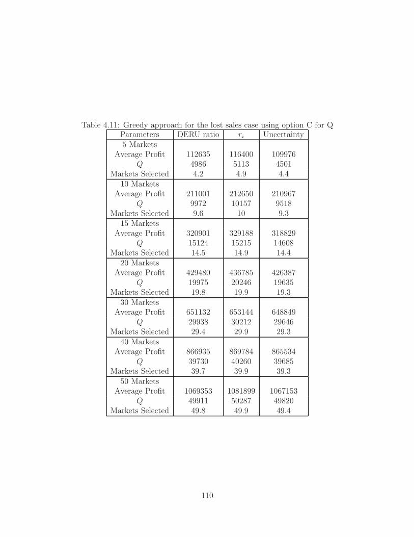
Table 4.11: Greedy approach for the lost sales case using option C for QParameters DERU ratio ri Uncertainty5 Markets

Average Profit 112635 116400 109976Q 4986 5113 4501


Average Profit 211001 212650 210967Q 9972 10157 9518

Markets Selected 9.6 10 9.315 Markets

Average Profit 320901 329188 318829Q 15124 15215 14608


Average Profit 429480 436785 426387Q 19975 20246 19635


Average Profit 651132 653144 648849Q 29938 30212 29646


Average Profit 866935 869784 865534Q 39730 40260 39685


Average Profit 1069353 1081899 1067153Q 49911 50287 49820


110

4.7 Conclusions

In this chapter we have presented various extensions to the so called “selective

newsvendor problem”. We have extended the horizon of research for studying the

SNP by including the market-specific expediting cost and the lost sales scenario. As

a conclusion, we have described our potential implementation approaches for each

of the extension. We developed three heuristic solution approaches for finding the

total order quantity for both the market-specific expediting cost and the lost sales

scenario. To find both the preferred market selections (as well as an associated order

quantity): We proposed an approach that examines solutions resulting from each of

several market rankings. We contribute to the research in the field of demand selection

by providing an optimal solution method for the rationing approach for distributing

shortages. We help managers to make more informed decisions by educating them the

sensitivity of the expected profit related to the changes in the different parameters

like costs and revenue.

The heuristic method for rationing provides solutions comparable to those ob-

tained when optimally solving with GAMS. The best solution by the greedy approach

for the market-specific expediting cost or for the lost sales scenario provides higher

expected profit as compared to the rationing approach. For the market-specific ex-

pediting cost, the rankings based on net revenue when provided best results for the

greedy approach. Similarly for the lost sales case, ranking based on per unit revenue

always provided best solutions for the greedy approach. However, ranking based on

demand variance always provided worst procurement policies among all the rankings.

For both extensions to the SNP, the heuristic based on the option when the total or-

der quantity is calculated using weighted critical fractile from the rationing approach.

In conclusion we provided a high quality constructive heuristic for distributing the

111

shortages via greedy approach.

One of the future work directions would be to consider the effect of correlated

demands. The correlation could be either negative or positive. Another future work

directions would be to study the impact on procurement policy if we have a limit on

Q in the expediting case, i.e., Q ≤ B. One can also study whether there are other

demand distributions such that this analysis is tractable (e.g., Uniform)?

112

Chapter 5

Conclusions

In this dissertation we present the various operational scenarios for the revenue

and order management under demand uncertainty. We contribute in the field of

demand selection by providing the decision maker in any firm with a tool set for

assessing the value of profit and risk, when obtaining solutions for the probabilistic

risk models can be quite cumbersome. Chapter 1 extensively explores the existing

literature in the field of stochastic demand management to review some fundamental

ideas. In Chapter 2, we present the risk averse selective newsvendor problem for

normally distributed demands. We continued our study on the risk averse selective

newsvendor problem in Chapter 3 for the various forms of demand distributions. In

Chapter 4, we revert back to basic selective newsvendor problem and present some

generalizations to this and open the new horizons of research in this particular field.

In Chapter 2, for the risk minimizing model, we introduced a constructive

heuristic that provides high quality solutions at a fraction of the time of an enumer-

ative approach. We point out that obtaining solutions to probabilistic risk models

can be quite cumbersome, and we offer approaches that firms dealing with risk issues

can implement. When there is no closed-form solution approach available for defining

113

the profit distribution (and worst-case profits), we must resort to an approach using

simulation as described in the Chapter 2. One future area of interest would be the

multi-period market or order selection problem with risk. This is a very rich area of

research with lots of opportunity.

In Chapter 3, we offer several alternate market selection and product ordering

models that vary in their inclusion of risk. We introduced an exact solution approach

to incorporate risk that uses Conditional Value-at-Risk via scenario analysis for AON

demands. We have tested potential market sizes from 5 to 15 for AON demands.

While we can analyze these cases in quite thorough detail, there is clearly motivation

for studying larger problem sizes. However, the problem suffers from the curse of

dimensionality, and the exact solution approach proposed in the current work becomes

intractable using CPLEX and Concert Technology. We have to consider heuristic

approaches to solving such problem sizes, determining upper bounds that can help

identify the quality of solutions produced by a heuristic.

Simulation analysis helped us to investigate the resulting profit distributions

for each of the demand distributions, which are again used in determining respective

procurement policies. As mentioned in the Chapter 3, all the results were more

influenced by the behavior of the heuristic (presented in Chapter 2) as compared to

demand distributions.

In Chapter 4, we extend the area of research for studying the SNP by includ-

ing the market-specific expediting cost and the lost sales scenario. As a conclusion,

we describe our potential implementation approaches for each of the extension. We

present an exact closed form solution for rationing approach for both generalizations

to the SNP. For both generalizations we formulated an optimization problem in the

form of mixed integer nonlinear problem and solved it using the lindoglobal solver

provided by GAMS software. In a greedy allocation approach, we develop the simula-

114

tion based heuristic solution approach for finding the optimal order quantity for both

the market-specific expediting cost and the lost sales scenario. For this heuristic, we

offer three different options to determine the total order quantity for the selected set

of markets. Thus, in effect we offer three heuristics. We also provide insights into

the quality of solutions from the heuristic against the ones obtained by solving the

exact optimization problem. One of the future work directions from here would be

to study the impact on procurement policy if we have a limit on Q in the expediting

case, i.e., Q ≤ B. One can also study whether there are other demand distributions

such that this analysis is tractable (e.g., Uniform)?

115

Bibliography

[1] L. Abdel-Malek, R. Montanari, and L. Morales. Exact, approximate and generaliterative models for the multi-product newsboy problem with budget constraint.IJPE, 91(2):189–198, 2004.

[2] V. Agrawal and S. Seshadri. Impact of uncertainty and risk aversion on priceand order quantity in the newsvendor problem. Manufacturing and Service Op-erations Management, 2(4):410–423, 2000.

[3] P. Artzner, F. Delbaen, J.M. Eber, and D. Heath. Coherent measures of risk.Mathematical Finance, 9:203–228, 1999.

[4] Y. Aviv. The effect of collaborative forecasting on supply chain performance.Management Science, 47(10):1326–1343, 2001.

[5] I.S. Bakal, J. Geunes, and H.E. Romeijn. Market selection decisions for inven-tory models with price-sensitive demand. Journal of Global Optimization, 2007.doi:10.1007/s10898-007-9269-3.

[6] M.S. Bazaraa, H.D. Sherali, and C.M. Shetty. Nonlinear Programming: Theoryand Algorithms. John Wiley & Sons, New York, New York, 2nd edition, 1993.

[7] D. Bertsimas and A. Thiele. A robust optimization approach to inventory theory.Operations Research, 54(1):150–168, 2006.

[8] J. Birge and F. Louveaux. Introduction to Stochastic Programming. SpringerSeries in Operations Research, New York, New York, 1997.

[9] S. Brealy and S. Myers. Principles of Corporate Finance. Irwin McGraw-Hill,New York, New York, 7th edition, 2002.

[10] C. Cachon. Competitive supply chain inventory management. In S. Tayur,M. Magazine, and R. Ganeshan, editors, Quantitative Models for Supply ChainManagement. Kluwer Academic Publishers, Boston, Massachusetts, 1999.

[11] S. Carr and I. Duenyas. Optimal admission control and sequencing in a make-to-stock/make-to-order production system. Operations Research, 48(5):709–720,2000.

116

[12] S. Carr and W. Lovejoy. The inverse newsvendor problem: Choosing an optimaldemand portfolio for capacitated resources. Management Science, 46(7):912–927,2000.

[13] K. Charnsirisakskul, P. Griffin, and P. Keskinocak. Order selection and schedul-ing with leadtime flexibility. IIE Transactions, 36(7):697–707, 2004.

[14] F. Chen and A. Federgruen. Mean-variance analysis of basic inventory models.Working paper, 2000.

[15] M. Chen and C. Chuang. An extended newsboy problem with shortage-level con-straints. International Journal of Production Economics, 67(3):269–277, 2000.

[16] X. Chen, M. Sim, D. Simchi-Levi, and P. Sun. Risk aversion in inventory man-agement. Working paper, Department of Mechanical and Industrial Engineering,2004.

[17] Tsan-Ming Choi, Duan Li, and Houmin Yan. Newsvendor problem with meanvariance objectives. In The Proceedings of 5th International Conference on Op-timization: Techniques and Applications, 2001.

[18] C. Chung and J. Flynn. A newsboy problem with reactive production. Computers& Operations Research, 28(8):751–765, 2001.

[19] R.A. Collins. The behavior of the risk-averse newsvendor for uniform, truncatednormal, negative binomial and gamma distributions of demand. Working paper,Santa Clara University, Department of Operations and Management InformationSystems, 2004.

[20] L. Dong and N. Rudi. Who benefits from transshipment? exogenous vs. endoge-nous wholesale prices. Management Science, 50(5):645–657, 2004.

[21] L. Eeckhoudt, C. Gollier, and H. Schlesinger. The risk-averse (and prudent)newsboy. Management Science, 41(5):786–794, 1995.

[22] G.D. Eppen. Effects of centralization on expected costs in a multi-location news-boy problem. Management Science, 25(5):498–501, 1979.

[23] S. Erlebacher. Optimal and heuristic solutions for the multi-item newsvendorproblem with a single capacity constraint. POMS Series in Technology andOperations Mangement, 9(3):303–318, 2000.

[24] J. Geunes, H.E. Romeijn, and K. Taaffe. Requirements planning with pricingand order selection flexibility. Operations Research, 54(2):394–401, 2006.

[25] J. Geunes, Z.J. Shen, and H.E. Romeijn. Economic ordering decisions withmarket choice flexibility. Naval Research Logistics, 51(1):117–136, 2003.

117

[26] J. Gotoh and Y. Takano. Newsvendor solutions via conditional value-at-riskminimization. European Journal of Operational Research, 179(1):80–96, 2007.

[27] G. Hadley and T. Whitin. Analysis of Inventory Systems. PH, 1963.

[28] B. Keren and J. Pliskin. A benchmark solution for the risk-averse newsvendorproblem. EJOR, 174:1643–1650, 2006.

[29] M. Khouja. The single-period (news-vendor) problem: Literature review andsuggestions for future research. Omega, 27:537–553, 1999.

[30] P. Kouvelis and G. Gutierrez. The newsvendor problem in a global market: opti-mal centralized and decentralized policies for a two-market stochastic inventorysystem. Management Science, 43(5):571–585, 1997.

[31] H.S. Lau. The newsboy problem under alternative optimization objectives. Jour-nal of the Operational Research Society, 31:525–535, 1980.

[32] Q. Li. Risk, risk aversion and the optimal time to produce. IIE, 39:145–158,2007.

[33] H.M. Markowitz. Portfolio selection. The Journal of Finance, 7(1):77–91, 1952.

[34] G.E. Monahan, N.C. Petruzzi, and W. Zhao. The dynamic pricing problem froma newsvendor’s perspective. Manufacturing and Service Operations Management,6(1):73–91, 2004.

[35] I. Moon and E.A. Silver. The multi-item newsvendor problem with a budgetconstraint and fixed ordering costs. Journal of the Operational Research Society,51:602–608, 2000.

[36] N.C. Petruzzi and M. Dada. Pricing and the newsvendor problem: A reviewwith extensions. Operations Research, 74:183–194, 1999.

[37] N.C. Petruzzi and G.E. Monahan. Managing fashion goods inventories: Dynamicrecourse for retailers with outlet stores. IIE Transactions, 35(11):1033–1047,2003.

[38] G. Pflug. Some remarks on the value-at-risk and the conditional value-at-risk.In S. Uryasev, editor, Probabilistic Constrained Optimization: Methodology andApplications, pages 272–281. Kluwer Academic Publishers, Dordrecht, 2000.

[39] E.L. Porteus. Stochastic inventory theory. In D. Heyman and M. Sobel, ed-itors, Handbooks in Operations Research and Management Science; Volume 2,chapter 12, pages 605–652. North-Holland, Amsterdam, The Netherlands, 1990.

118

[40] A. Prekopa. Stochastic Programming. Kluwer Academic Publishers, Dordrecht,The Netherlands, 1995.

[41] R.T. Rockafellar and S. Uryasev. Optimization of conditional value-at-risk. TheJournal of Risk, 2(3):21–41, 2000.

[42] R.T. Rockafellar and S. Uryasev. Conditional value-at-risk for general loss dis-tributions. Journal of Banking and Finance, 26(7):1443–1471, 2002.

[43] H.E. Romeijn, J. Geunes, and K. Taaffe. On a nonseparable convex maximizationproblem with continuous knapsack constraints, 2006. Forthcoming in OperationsResearch Letters.

[44] M.E. Schweitzer and G.P. Cachon. Decision bias in the newsvendor problem witha known demand distribution: experimental evidence. Management Science,46(3):404–420, 2000.

[45] A. Sen and A.X. Zhang. The newsboy problem with multiple demand classes.IIE Transactions, 31:431–444, 1999.

[46] S. Sen and J.L. Higle. An introductory tutorial on stochastic linear programmingmodels. Interfaces, 29:33–61, 1999.

[47] R.A. Shumsky and F. Zhang. Dynamic capacity management with substitution.Working paper, Tuck School of Business, Dartmouth University, 2005.

[48] E. Silver, D. Pyke, and R. Peterson. Inventory management and productionplanning and scheduling. JWILEY, NY, 3rd edition, 1998.

[49] M. Steinbach. Markowitz revisited: mean-variance models in financial portofolioananlysis. SIAM Review, 23(1):31–85, 2001.

[50] K. Taaffe. Single airport ground holding problem - benefits of modeling uncer-tainty and risk. In P. Pardalos, A. Migdalas, and G. Baourakis, editors, SupplyChain and Finance. World Scientific, River Edge, New Jersey, 2004.

[51] K. Taaffe and J. Geunes. Models for integrated customer order selectionand requirements planning under limited production capacity. In P. Pardalos,A. Migdalas, and G. Baourakis, editors, Supply Chain and Finance. World Sci-entific, River Edge, New Jersey, 2004.

[52] K. Taaffe, J. Geunes, and H.E. Romeijn. Capacity acquisition and stochasticcustomer demand assignment in a network of facilities. In Proceedings of IIEResearch Conference, Atlanta, Georgia, 2005.

119

[53] K. Taaffe, J. Geunes, and H.E. Romeijn. Target market selection and marketeffort under uncertainty: The selective newsvendor problem. European Journalof Operational Research, 189(3):987–1003, 2008.

[54] K. Taaffe and H.E. Romeijn. Selective newsvendor problems with all-or-nothingorder requests. In Proceedings of IIE Research Conference, Atlanta, Georgia,2005.

[55] K. Taaffe, H.E. Romeijn, and D. Tirumalasetty. A selective newsvendor approachto order management. Working paper, Department of Industrial Engineering,Clemson University, 2007.

[56] K.M. Taaffe and D. Tirumalasetty. Identifying demand sources that minimizerisk for a selective newsvendor. In M.E. Kuhl, N.M. Steiger, F.B. Armstrong,and J.A. Joines, editors, Proceedings of the 2005 Winter Simulation Conference,pages 1898–1905, Orlando, Florida, 2005.

[57] B. Tomlin and Y. Wang. Deterministic production planning with concave costsand capacity constraints. Manufacturing and Service Operations Management,7(1):37–57, 2005.

[58] A. Tsay, S. Nahmias, and N. Agrawal. Modeling supply chain contracts: Areview. In S. Tayur, M. Magazine, and R. Ganeshan, editors, QuantitativeModels for Supply Chain Management. Kluwer Academic Publishers, Boston,Massachusetts, 1999.

[59] S. Uryasev. Conditional value-at-risk: Optimization algorithms and applications.Financial Engineering News, 14(2), 2000.

[60] J.A. Van Mieghem. Risk-averse newsvendor networks: Resource sharing, sub-stitution, and operational hedging. Working paper, Northwestern University,Kellogg School of Management, 2004.

[61] C.X. Wang and S. Webster. The loss-averse newsvendor problem. Omega, 2006.doi:10.1016/j.omega.2006.08.003.

[62] J. Wu, J. Li, S. Wang, and T.C.E. Cheng. Mean-variance analysis of the newsven-dor problem with stockout cost. Omega, 2008. doi:10.1016/j.omega.2008.02.005.

[63] S. Yang, J. Yang, and L. Abdel-Malek. Sourcing with random yields andstochastic demand: A newsvendor approach. Computers & Operations Research,34(12):3682–3690, 2007.

120

revenue and order management under demand uncertainty

Documents