return reversal in uk stocks - ivey business school · 2 return reversal in uk shares© glen c....
TRANSCRIPT

1
Return reversal in UK shares
Glen C. Arnold and Rose D. Baker
Centre for Economic and Finance Research
Salford Business Sschool,
University of salford
Salford,
Manchester,
M5 4WT, UK
Email: [email protected]
Salford Business School Working Paper Series
Paper no. 107/07
17 January 2007

2
Return reversal in UK shares©
Glen C. Arnold and Rose D. Baker
Salford Business School Working Paper
ABSTRACT
We observe systematic long-term reversal of share returns for companies listed on the London
Stock Exchange over the period 1960-2002. Loser shares (the worst performing shares in the
prior five years) out-perform winner shares (the best performing shares over the prior five years)
by about 14% per year. By separating the firm size effect from the return reversal effect we show
the presence of both. This evidence is in direct contradiction to Clare and Thomas (1995), who
found no return reversal following an adjustment for size. Return reversal is a feature of large as
well as small companies. A seven-part consideration of risk does not substantiate the argument
that loser out-performance is compensation for risk.
JEL classification: G14, information and market efficiency
Key words: Return reversal, Overreaction, Market inefficiency, Market efficiency

3
1. Introduction
A strong return reversal effect has been shown in US studies (e.g. De Bondt and Thaler,
1985, 1987; Chopra, et. al., 1992). That is, portfolios of shares showing the worst total return
performance over a three or five year period subsequently significantly out-perform portfolios of
shares made up of prior period „winners‟, and the market portfolio, over the long horizon. This
out-performance is remarkably high: extreme prior losers out-perform extreme prior winners by
5-10 per cent per year. Studies from around the world have drawn similar conclusions1.
Contradicting the consensus developed in the US and elsewhere, in 1995 Clare and
Thomas published the most comprehensive analysis to that date of UK shares, and concluded
that the return reversal effect disappeared if the influence of market capitalization (size effect) is
adjusted for. Thus, we have doubt thrown on belief in the generality of the return reversal effect.
If it is not present in the second most important stock market in the world where does that leave
the argument that share returns tend to go into reverse across markets and at various points in
stock market histories? Are the reported results a product of mining data in particular markets in
specific time periods?
Clare and Thomas‟ work, however, suffered from some serious methodological flaws.
This paper provides a more robust analysis. It also extends the study period to 48 years, ending
in 2002, rather than 1990, permitting us to observe the phenomenon at the height of the bull
market. Our results indicate the presence of an economically significant return reversal effect in
the UK share market. Moreover, it is unlikely that this effect can be attributed to the influence of
size or risk. We find that extreme losers outperform extreme winners by about 14% per year in
the five years following portfolio formation. The effect is present in both the full sample and in
the largest 20% of firms, but is stronger for smaller companies.
2. UK Empirical Studies

4
In comparison with the US there have been few studies of return reversal in UK shares.
Those that are available differ in the period studied, length of study and methodology used.
Power, Lonie and Lonie (1991) take the list of the „top 200‟ UK companies in the June 1982
edition of Management Today. They calculate the share price changes plus dividends for each
company over the 10 years to 1982. The 30 best performing companies are assigned to a winner
portfolio. The bottom 30 companies combine to form a loser portfolio. They report positive
cumulative abnormal returns for prior-period losers of 86% in the five-year test period, while the
prior-period winners showed negative abnormal returns of -47%.
The study by MacDonald and Power (1991) cumulates market-adjusted excess return
over three year formation periods. The winners are defined as the top 5% of firms and the losers
as the bottom 5%. They establish eight sets of portfolio formations at three-year intervals
between 1959 and 1985, and examine cumulative excess returns of the portfolios over three year
holding periods. They find a reversal in the performance of the winner and loser portfolios in the
test period. The average cumulative abnormal return from the arbitrage strategy of selling short
the shares in the winner portfolios and buying shares in the loser portfolios is a statistically
significant 29.15%. However, MacDonald and Power (1993) examine the predictability of 40
individual UK shares over the period 1982 to 1990 and conclude that rather than return reversal,
„for the vast majority of the firms in the sample, share prices appear to follow a random-walk
process….the findings of this paper, therefore, would appear to lend support to the proponents of
a traditional view of stock market efficiency‟. (p.38)
Clare and Thomas (1995) declared, after examining a random sample of up to 1000
shares between 1955 and 1990, that losers outperform winners by a statistically significant 1.7%
per annum, “However, after controlling for firm size we find that this return difference can be
explained by the small firm effect. Our findings thus provide no evidence of overreaction in the
UK stockmarket” (p.963). There are a number of problems with their approach, which, when

5
combined, may help to explain why they were unable to detect return reversal. First, they tested
only six series of portfolio returns (six portfolio formations) for periods of three years. We argue
that many more portfolios need to be formed and tested to gain insight into the persistence of
return reversal. This study examines 39 portfolio formations over 12, 24, 36, 48 and 60 month
holding periods. Second, their method of adjusting for size lacked sensitivity – we undertake a
more comprehensive and sensitive analysis separating the return reversal effect from the size
effect. Third, Clare and Thomas required firms to be “continuously quoted” to be included in
their sample. As they freely admit, this introduced survivorship bias. Fourth, they used quintile
portfolios, rather than deciles, leading to less sensitive tests. Fifth, they only examined portfolios
formed by equally weighting the constituent shares, rather than considering the impact of value
weighting within the portfolios. Sixth, Clare and Thomas used cumulative abnormal returns
(CAR) rather than buy-and-hold returns to measure both formation and test period returns.
Given the extensive literature describing the distortions caused by the use of CARs in long-run
studies (e.g. Dissanaike, 1994, Barber and Lyon, 1997) it is important that the data be analysed
using the buy-and-hold method
Dissanaike (1997, 2002) conducts an analysis of return reversal, extending the test
periods to 48 months. He shows return reversal for eight out of the ten portfolio formations
examined even after adjustment for firm size. However he left open the question of whether the
return reversal effect is evident in the entire cohort of London Stock Exchange (LSE) listed
companies, because only those companies in the FT 500 share index (the largest 500 by market
capitalization) are included in these studies. Following the imposition of the condition that only
those companies without missing returns over the prior 48 months are included he was left with
an average of 450 companies in each formation year. Dissanaike focused on returns on
portfolios formed over the short period between 1979 and 1988. It is possible for sceptical
readers to draw the conclusion that this evidence of a tendency for loser firms to outperform

6
winner firms can easily be explained away as an event occurring in the 1980s, and so does not
pose an overwhelming challenge to the efficient markets hypothesis.
Campbell and Limmack (1997) in examining portfolios of loser companies and portfolios
of winner companies found, over a five year period following portfolio formation, that a
“reversal in the abnormal returns of winner and loser portfolios was experienced over each of the
years 2-5, thus lending support to the winner-loser effect” (p.537). In their study the companies
are defined as winners and losers on the basis of abnormal returns calculated over only 12
months. This is unusual in the „long-term‟ return reversal literature, given that prior period
returns are generally calculated over 3 or 5 year periods.
In sum, the studies reported in the literature have produced somewhat conflicting results.
It seems clear that there is a return reversal effect, but its size is unclear, and the question of
whether it is subsumed by the firm size effect remains.
It is therefore important to ascertain the strength of the return reversal phenomenon when
a larger data set and up-to-date analytical techniques are employed. This paper extends the study
period to 48 years, ending in 2002, permitting us to observe the phenomenon at the height of the
recent bull market as well as observing the strength of return reversal in each of the decades from
the 1960s to the 1990s, thereby gaining a much broader picture. In all, this study examines 39
portfolio formations, far more than any previous paper. Furthermore, test period market-adjusted
returns are reported for 12, 24, 36, 48 and 60 months.
In addition to using the buy-and-hold method to analyse the data we extend the analysis
further by considering market capitalization weighting within portfolios and examine returns
against both an equally weighted and a value weighted market portfolio. In addition, these
portfolios are formed from companies ranked by prior period returns and formed into deciles,
leading to a more sensitive test than a quintile based analysis. The survivorship bias problem is

7
dealt with by including all firms in the sample whether or not they are liquidated during the test
period.
We perform two tests to separate the size effect from the return reversal effect and
conduct a seven-part consideration of risk, which includes making use of the Fama and French
three-factor model (1993, 1996). This paper also contributes to the literature by observing the
return reversal effect in both large and small firms.
3. Hypotheses
We test the following hypotheses:
o On average shares that exhibit extreme negative movements in returns over a period of
five years will, during the subsequent five years, experience high returns relative to both
the market index and to those shares that produced very high returns in the prior five-year
period.
o The more extreme the return in the prior five years, the greater will be the subsequent
adjustment.
o The reversal of return performance is explained by additional risk carried by the extreme
loser shares.
o The return reversal effect is subsumed by the size effect.
o The return reversal effect is present in the investible universe relevant for most
institutional investors, i.e. in the largest 20% of companies, as well as in the small
company cohort.
4. Return reversal and overreaction
The term overreaction has become so linked with the phenomenon of long-term share
return reversal that this area of study has become known as the overreaction literature. However,

8
it is important to maintain the distinction between the observation of share return reversals and
the concept of overreaction. The two may be consistent with each other, and may provide
mutually supportive evidence, but they have different roots and meanings. The study of return
reversal is the examination of time series share (strictly, share portfolio) relationships, and the
untangling of this effect from other potential explanations for patterns observable in the data,
such as the size effect, or the impact of beta risk.
The overreaction discussion owes its origin to departures from Bayesian rationality
documented in the field of experimental psychology. The Bayesian hypothesis for learning is for
the consistent use of conditional probabilities for changing beliefs on the basis of new
information. It would seem that such high levels of rationality are not an accurate
characterization of how individuals behave when faced with new data (Kahneman et al., 1982,
Kahneman and Tversky, 2000). Individuals, when revising their beliefs, tend to overweight
recent information and underweight prior (or „base-rate frequency‟) data. They often fall victim
to the representative heuristic (Tversky and Kahneman, 1971, 1974, Kahneman and Tversky,
1972, Arrow 1982) under which an individual judges the likelihood of a future event by the
similarity of the present (recent) evidence to it.
In behaving this way decision takers fail to properly allow for the necessity of moderating
extreme predictions. They overreact to recent unexpected, dramatic and salient news. Grether
(1980), for example, found this in his laboratory experiments with students. Gilovich et al.
(1985) found it in the sports market, where players and fans of basketball believe that a player is
more likely to hit a shot if his previous shot was a hit, despite the evidence of a lack of
correlation between successive shots. Clapp and Tirtiroglu (1994) found positive feedback in the
housing market where recent rates of change become over weighted information used by
decision-makers. There are many more examples in a wide variety of fields. Coming back to
finance, it has been observed that the actions of professional security analysts, private investors

9
and institutional fund managers display behaviour consistent with this overreaction view; for
example, Dreman and Berry (1995), Dreman (1998), Bauman et al. (1999) and Dreman and
Lufkin (2000) observing returns on value and growth shares, and Stein (1989) in the options
market.
When applied to share return patterns the overreaction interpretation is as follows. Winner
shares build a reputation over many years for high performance, usually based on corporate
performance, such as abnormal rises in earnings per share. The winners are subject to greater
publicity than other shares. Their high quality image and acclaim are not readily dissipated.
These acknowledged „good companies‟ are also regarded as „good shares‟ to hold. They become
overvalued. On the other hand loser companies, with a history of disappointing results, are
stereotyped as forever on a downward course. The overreaction of investors leads to under-
valuation after investors become excessively pessimistic.
For both the winner and the loser shares investor judgment on future performance is
„anchored‟ on recent historic performance. Investors fail to allow sufficiently for the base-rate
data, which show a tendency for company earnings growth to revert to the mean, i.e. those
showing particularly strong growth in the past show weaker growth in the future, while those
with an extreme declining pattern over many years tend to show an increasing profit trend
(Little, 1962; Whittington, 1971, 1972, 1978; Mueller 1977; DeBondt and Thaler 1987; Power,
Lonie and Lonie 1991; Fuller et al. 1993; Power and Lonie, 1993; Chan et al., 2003). As
investors observe the improving position of the losers and the worse than anticipated pattern in
the winners their stereotyping and anchoring is gradually eroded. Share prices begin to move in
the opposite direction, resulting in the mean reverting pattern of share returns.
This paper reports evidence showing the presence of a strong return reversal effect in the
UK, persistent over four decades and robust to adjustment for the size effect and to various
measures of risk. The results are consistent with the theory of overreaction, but do not, in

10
themselves, prove that the cause of the pattern in share returns is overreaction. We merely
suggest that the overreaction hypothesis is a parsimonious explanation for the empirical
observations. However, the alternative explanation for the data pattern we observe, namely
compensation for additional risk bearing, seems less plausible than overreaction, given the
strength of our results.
5. Data, Sample Selection and Method
Monthly return data are taken from the London Share Price Data (LSPD) for the period
January 1955 to December 2002. This provides returns for every share listed on the London
Stock Exchange, LSE, in the period 1975-2002. For the first 20 years of the study period (1955
to the end of 1974) the LSPD provides returns for only one-third of the listed companies; these
are randomly selected2. The analysis includes all the shares in the one-third random sample for
the period January 1955 to December 1974 and all the LSE listed companies thereafter, except
investment trusts and foreign companies in both periods. The firms on the lightly regulated
markets operated by the LSE (The Alternative Investment Market, Third Market or the Unlisted
Securities Market) are not “listed” and so are excluded from the analysis. Companies on OFEX
and the O.T.C. market are also excluded.
All shares continuously listed for the prior five calendar years are ranked each year on the
basis of their five-year buy-and-hold returns and assigned to one of ten portfolios. The first
ranking period ends at the end of December 1959, and the last one ends at the end of December
1997, a total of 39 ranking periods. Portfolios are formed at the beginning of January each year
from 1960 to 19983.
Test period buy-and-hold returns for a portfolio are calculated from individual monthly
share prices and dividend payments, allowing for stock splits and other capital changes4 5. The
returns for a portfolio are then market adjusted, either by an equally weighted market index or by

11
a market capitalization (value) weighted market index. We examine the portfolio performance
both when the portfolio shares are equally weighted within the portfolio and when they are
weighted by market capitalization within the portfolio. Under market capitalization weighting
each firm‟s weight is expressed as a proportion of the total market capitalization of all the firms
in the decile portfolio at the date of portfolio formation. We first report equally weighted returns
for each portfolio as this more closely represents a strategy implementable by all but the largest
of investors. The effect of value weighting within the portfolios is to reduce the return premium
to losers owing to the tendency of losers to be smaller firms. This leads to the reporting of the
most conservative results. These may also be the results of most interest to the large investors
who might allocate portfolio funds by market capitalisation.
Shares whose type of death from the LSPD database is described as liquidation (death
code type 7) quotations cancelled for reasons unknown (14), receiver appointed/liquidation (16),
in administration/administrative receivership (20), and cancelled assumed valueless (21), are
regarded as losing all value in the delisting month. However, if there is a post-liquidation
dividend this is invested equally among the remaining shares in the portfolio. By including even
those companies that delist during the test period, many of which show a –100% return, we
avoid survivorship bias.
If a company is deleted from the LSPD database for any of the following reasons the
money received (or value of shares or other securities received) is reinvested in the portfolio on
an equally weighted basis. That is, the remaining investments in the portfolio are scaled up:
- Acquisition/takeover/merger (5)
- Suspension/cancellation with shares acquired later (6).
- Quotation cancelled as the company becomes a private company (8 and 9)
- Quotation suspended (10)
- Voluntary liquidation (11)

12
- Change to foreign registration (12)
- Quotation cancelled for reason unknown, dealings under rule 163 (13)
- Converted into an alternative security for the same company (15)
- Nationalisation (18)
If the amount received from these deletions is unknown then the last share value on LSPD is
used as the amount available to invest in the shares remaining in the portfolio.
The number of firms in the sample grows from 925 in the first sample selection year
(1960) to 1152 in the last year (1998). The peak year is 1980 with 1594 firms. On average the
sample comprises 810 firms over the portfolio formation years 1960 to 1979 (when a one-third
random sample of shares is used) and 1240 firms for the portfolios formed from 1980 to 1998,
when all listed ordinary shares are included.
Finally, throughout this paper returns are calculated as the proportional changes in share
value over a period, except in the calculation of betas, where continuously compounded returns
are used.
6. Average performance across portfolio formations
In this section we report average results over the 39 test periods for each of the decile
portfolio market-adjusted returns. The market index, used to adjust returns, comprises all shares
in the sample. Table 1 shows a striking inverse relation between the past and subsequent returns.
When equal weights are used for both within the portfolio and for the market index (the method
commonly used in previous studies) we find that the loser portfolio out-performs the market by
53% over five years, or 8.9% per year. In contrast, the prior period winners under-perform in the
subsequent five years by 47%. If the market index is constructed on the basis of value weighting
(in a similar manner to the FTSE 100 or the FTSE All Share index) the results are even more

13
dramatic for the loser portfolio. Now, with a greater weight given to the largest companies in the
index, the loser portfolio out-performs the index by 109% over five years or 15.9% per year.
The difference between the results shown in the two parts of panel A suggest a strong size effect
(Banz (1981), Dimson and Marsh (1986, 2001)) in the UK share market given the lower index
returns when greater weight is given to large companies. The influence of the size effect is
explored in section 11 of the paper.
Decile performance rank is remarkably well ordered in panel A: the highest test period
returns are from portfolio 1 and the lowest from portfolio 10; all the other deciles are in the
expected order over both four and five year test periods. This adds considerable support to the
overreaction hypothesis, as it shows that return reversal is not confined to the extreme cases. All
the return differentials in panel A (equal-weighted market index) are statistically significant at
the 1 per cent level for test period years four and five except for portfolios 3, 4 and 5. Consistent
with overreaction the middle portfolios do not show market-adjusted returns significantly
different from zero, because at the time of portfolio formation they are not expected to be subject
in any significant way to either over-optimism or over-pessimism.
Anomalies in long-term share price behaviour have been observed to diminish or
evaporate when firms within the portfolio under study are value weighted. For example Fama
(1998) notes: “we find that apparent anomalies in long-term post-event returns typically shrink a
lot and often disappear when event firms are value-weighted rather than equal-weighted. One
can argue that value-weight returns give the right perspective on an anomaly because they more
accurately capture the total wealth effects experienced by investors” (p.296). The smallest firms
in the portfolio may be creating most of the effect. By moving away from equal weighting to
value weighting the influence of very small firms is reduced. If, by switching to value weighting
within the decile portfolios we find that the abnormal returns on the loser and winner portfolios
are greatly reduced we can plausibly argue that the anomaly is driven mainly by the over-

14
weighting of small and micro-firms within the deciles. Panel B shows the results of this
analysis. We find very similar results to those shown in panel A for the extreme portfolios; the
numbers being only slightly less when the portfolios are value weighted. However, the ranking
of the 10 portfolios is less well behaved, particularly in the case where the market portfolio is
constructed by equal weighting; for example, portfolio 10 (winner) shows a higher return than
portfolio 9.
TABLE 1 HERE
The month-by-month average cumulative market-adjusted returns for the portfolios are
shown in Figure 1. These are calculated by equally weighting within the deciles and by market
adjusting with an equally weighted market index. Throughout the post-formation period the
performance of each portfolio is positioned vis a vis other portfolios as we would expect under
the overreaction hypothesis. That is, from the outset the most extreme formation period losers
become the highest performers in the test period. Portfolio 2 takes second place, followed by
portfolio 3, and so on, down to the winner portfolio being the worst.
FIGURE 1 HERE
7. Large firm analysis
Chopra et al. (1992) find no return reversal effect in larger firms: „for the largest 20% of
the NYSE firms (roughly the S&P 500) no overreaction effect is apparent.‟ (p.256). Chopra et al.
go on to argue that this evidence is consistent with the hypothesis that individuals, who tend to
be the primary holders of smaller firms, overreact, whereas institutions, the dominant holders of
larger firms do not. We examine the largest 20% of UK listed firms in the sample (by market
capitalization). The evidence shown in Table 2 is the start of a series of results (the remainder
shown in section 11), which address the critique that the return reversal effect is explained by the
small firm effect.

15
The data in Table 2 is constructed in the same way as Table 1 except that only the largest
20 per cent of companies (at portfolio formation dates) are included in the deciles. Examining
the ranking period data first, we find that the returns prior to portfolio formation are less extreme
than those for the all-company analysis. For example, whereas the loser portfolio constructed
from companies of all sizes has a five-year market-adjusted ranking period return of –227%6,
the corresponding return for the loser portfolio comprising the largest 20% of companies is a
mere -30%. For the winner portfolio the figures are somewhat closer together: 391% compared
with 581%. By focusing on the larger companies we tend to exclude those firms with the most
extreme prior period returns. This is especially the case for losers, because if a company shows a
large negative return it simply falls out of the top 20% at the portfolio formation date so that only
the moderate losers are included in the analysis in Table 2. This makes the large company
analysis a particularly tough test for return reversal and overreaction because it is reasonable to
expect it to be most apparent in the extreme losers and winners, rather than moderate losers and
winners.
When the test period returns of portfolios containing only large firms are compared with
an index comprising shares of all sizes we might expect, given the small firm effect, that these
portfolios will generally under-perform the index. This is indeed the case, as shown on the left
side of Table 2, where no portfolios produce statistically significant positive market-adjusted
returns. There is, however, a clear downward trend in performance as we move from portfolio 1
to portfolio 10. The difference in return between losers and winners over five years is 71% when
the shares within the portfolio are equally weighted and 92% when they are value weighted7. If
we market adjust returns using an index that gives much greater weight to large companies, and
is therefore closer to the size profile of the companies in the decile portfolios in Table 2, we find
a much clearer superiority of the loser portfolio to the market – shown on the right side of Table
2, where losers out-perform by 61% or 89%.

16
Overall, the results from Table 2, while not as strong as those in Table 1, nevertheless
demonstrate a return reversal effect in the largest companies listed on the LSE. Perhaps the
supposition that institutional investors are less susceptible to overreaction is suspect. Perhaps
professional investors are less resistant to cognitive errors, such as the representativeness
heuristic (Tversky and Kahneman, 1971, 1974, Kahneman and Tversky, 1972, Arrow, 1982)
than they like to think. This is certainly an opinion held by a number of experienced investors,
for example, Graham (1973, with Dodd, 1934), Buffett (1986), Lynch (1989) and Dreman
(1998).
TABLE 2 here
8. Reliability of the loser and loser minus winner strategy
Establishing the superior profitability of the loser strategy on average over the second
half of the twentieth century, while fascinating, is insufficient for practitioners and academics
alike. A key fact we need to know is whether there are long periods when the strategy fails to
pay-off. An investor, individual or institutional, needs to know that the strategy is fairly
consistent in providing high returns. Many investors are not prepared to accept even two
consecutive years of under performance, regardless of the out-performance over decades.
Financial economists, in order to comment on implications of the evidence for the debate on the
pricing efficiency of the LSE, need to know whether loser shares under-perform winner shares
with some regularity. This is of particular interest in poor states of the world, such as down
markets or economic recessions, when the marginal utility of consumption is high, making loser
shares unattractive to risk averse investors (Lakonishok et al. 1994).
We record in Figures 2(a), 2(b) and 2(c) the formation years that are followed by positive
or negative five-year returns for the loser-winner portfolio. In addition we show the years when
there was a bear market (defined as a negative real return for the calendar year), or when gross

17
domestic product growth is negative, to see if poor performance is particularly prevalent in these
bad states of the world. Given the space constraints of this paper the figures only show the
results for three strategies over five years. The results for alternative weightings within the
portfolio and for alternative weightings within the market index are available from the authors.
They show similar results. Also available are the results for each individual portfolio formation
when the test periods are 1, 2, 3, and 4 years. In all, 40 analyses were carried out: 4
combinations of weightings x 2 samples (all companies or large companies only) x 5 test period
lengths.
The figures show an overwhelming preponderance of positive returns over the five years
following portfolio formation. When value weighting is used (Figure 2 (b)), however, there is a
cluster of formations in the 1970s where winners out-performed losers. An investor allocating a
fund on the basis of market capitalisation would have suffered a frustrating period in the late
1970s and early 1980s as four of these arbitrage portfolios lose money8. This introduces a form
of risk to which the typical investor may conceivably be so averse that the high returns to the
repeated use of the loser-winner strategy over a decade or more are merely a rational reward for
accepting this risk – the portfolios produce an „expected return‟. This is an extreme
interpretation of the risk return trade-off, but we cannot completely discount it. Turning to the
largest 20% of companies (Figure 2 (c)) we find, again, a generally positive picture. However,
there is an obvious lengthy cluster of negative returns during the late 1980s and early 1990s,
where going short on the winners and long on the losers produced a loss. We see no obvious
relationship between performance of the loser-winner arbitrage portfolios and either market
downturns or recessions.
Table 3 shows the number of occasions when the loser portfolios produced negative
market-adjusted returns over five years. It also shows the number of occasions when the loser-
winner strategy failed to pay-off. Examining the results for the full sample, we find the strategy

18
of investing in the loser portfolio produces abnormally high returns in the majority of years in
each of the decades, 1960s, 1970s and 1990s. However, the evidence for the 1980s is more
mixed, with up to six of the loser portfolio formations producing sub-market returns. For both
the full sample and for the largest companies, when the decile portfolios and the market
portfolios are both calculated using value weighting, the loser portfolio under-performs the
market around one-quarter of the time. Thus, the strategy is fairly, but not completely, reliable.
The failure to out-perform in one out of four occasions may be sufficiently off-putting to
investors to explain the overall out-performance of losers. Perhaps, rather than a „rational‟
response to the risk of occasional under-performance, myopic loss aversion (Benartzi and Thaler,
1995) has a role to play here. Investors are unreasonably sensitive to short-term losses and they
evaluate their portfolios frequently, e.g. monthly or yearly, resulting in a demand for large
premiums to accept variability in return.
FIGURE 2(a) here, FIGURE 2(b) here, FIGURE 2(c) here, TABLE 3 HERE
9. Deletions and liquidations
Firms that have lost market value over a five-year period are more likely to be delisted in
the subsequent five years. The higher rate of firm attrition through deletion in the test period for
loser portfolios than for winner portfolios is evident in Table 4. Of the 95.6 companies that on
average comprised the loser portfolios at portfolio formation only 59.9 remained quoted 5 years
later. The most significant reason for removal from the loser portfolio is that the firm merged or
was taken over (21.9 out of the 35.7 firms deleted). Within 60 months 11.3 or 11.8% of the loser
decile companies on average (across 39 portfolio formations) failed compared with only 3% of
the winner portfolios. Despite one-eighth of the stocks in the loser portfolios falling into
liquidation and providing a significant downward push to the portfolio test period performance,
these portfolios still out-performed due to the exceptional returns gained on the survivors.

19
However, if investors are particularly sensitive to experiencing 11.8% of their portfolio running
into extreme financial distress then the risk explanation, based on distress, for the out-
performance of loser shares may have some support from these results (Chan and Chen (1991),
Fama and French (1996) refer to financial distress risk).
An interesting observation is that between one-fifth and one-quarter of companies merge
within five years, and the merger rate does not follow any discernable pattern across rank period
return deciles.
TABLE 4 HERE
10. Further risk tests
Various authors have argued that return reversals are due to investors rationally requiring
higher returns on loser shares and lower returns on winners due to a difference in risk. One
argument is that leverage change over the rank-period as a result of diminishing (increasing)
equity capital values for losers (winners) produces changes in equilibrium-required returns. A
series of negative abnormal returns increases the equity beta of loser firms, thus raising expected
return (e.g. Chan (1988), Ball and Kothari (1989)). Winners experience a decrease in equity
betas as leverage falls over the rank period and therefore have lower equilibrium expected
returns9. Chan (1988) also suggests that the risk of the loser firm may increase because of the
loss of economies of scale and the increase in operating leverage, which will be reflected in the
share‟s CAPM-beta.
In this section we further explore whether loser portfolios are indeed fundamentally
riskier than winner portfolios. We examined two forms of risk above: the frequency with which
loser or loser-winner strategies under-perform and the risk of liquidation. We now broaden our
analysis by examining risk in five additional ways. As well as considering beta and standard
deviation we observe the performance of the portfolios in months (rather than years) of poor and

20
good stock market return and during quarters (rather than years) of low and high economic
growth. We also apply Fama and French‟s three-factor model.
10.1. Worst stock market months and worst GDP quarters.
Exploring the risk of the portfolios by examining five-year returns, while interesting, is
incomplete. Conceivably, loser portfolios could perform well over the entire five years, but be
subject to severe declines for particular periods within those five years. Perhaps when there are
large declines in the stock market index over a period of a month the returns on the loser
portfolios fall to an exaggerated extent, showing them to be more risky than both the market and
the winner portfolio. Perhaps when quarterly real GDP declines the loser portfolios suffer more
than other shares.
Thus an investor with a time horizon of less than five years might be concerned about
these kinds of intra-year vulnerability to events. To test the risk of portfolios over short periods
we observe returns on the loser and winner portfolios as well as the market portfolio during each
of the 516 months from January 1960 to December 2002. These month are placed into four
categories:
o The 50 months when the value-weighted market index return was at its worst („W50‟)
o The other 137 months when the value-weighted market index fell („N137‟)
o The 50 months with the highest value-weighted market index returns („B50‟)
o The other 279 months when the value-weighted market portfolio rose („P279‟)
Each of the 60 test months for each of the 39 portfolio formations are allocated to one of the four
categories. The raw (not market adjusted) returns for each of the portfolios falling in a particular
month are observed. For any one month between January 1960 and December 2002 the
maximum number of portfolios held is five, but this can fall to as low as one in 1960 and in
21
2002. There are 516 possible observations months and 39x60 = 2340 monthly returns
observable for those months amounting to an average of 4.53 observed returns per month.
A similar analysis is conducted for the worst and the best quarters as measured by real
GDP growth. Quarterly real GDP data are obtained from Datastream. The 172 quarters are
allocated to the following categories:
o The 25 poorest real GDP growth quarters („W25‟)
o The next 61 lowest real GDP growth quarters („L61‟)
o The 25 best real GDP growth quarters („B25‟)
o The next 61 highest real GDP growth quarters („H61‟)
The returns for each of 60 months for each portfolio are allocated to one of the four categories
depending on the real GDP growth in the relevant quarter. The monthly portfolio returns falling
in a real GDP category are averaged for all months in that category.
In a separate analysis the monthly returns on the loser and winner portfolios are matched
up with the changes in real GDP for one quarter ahead, given the evidence indicating that the
stock market leads real GDP by approximately one quarter.
Panel A of Table 5 presents the performance of portfolios in various months as defined by
the extent of the rise or fall in the market index that month. The average difference in returns
between the loser and winner for each state is also reported along with t-statistics for the test that
the difference of returns is equal to zero. The results show that losers out-perform winners in all
states of the market (although the results are statistically insignificant for the best 50 months).
The largest difference is for the worst stock market months, followed by other negative index
months. This evidence does not support the view that losers are riskier than winners10
.
Panel B of Table 5 provides information on returns in various states of the world as
defined by real GDP growth in the quarter. The results show, again, that losers perform better
than winners in all states. This time, however, the largest difference in returns is during the best

22
GDP growth quarters, and the difference between losers and winners in the worst 25 quarters is
statistically indistinguishable at the 90% confidence level. Panel C shows the results if the
monthly returns on the loser or winner portfolio are matched up with the real GDP growth one
quarter ahead. The results do not alter the general conclusion that we find no evidence in Table
5 supporting a conventional asset pricing equilibrium in which the higher returns on the loser
portfolio are compensation for the under-performance in bad states of the world risk – it would
seem that the loser strategy does not expose investors to greater downside risk.
TABLE 5 HERE
10.2. Beta and standard deviation
Table 6 presents betas and standard deviations for each of the decile portfolios. Annual
returns data from the test period are used because of the problems associated with the use of
rank-period data to compute betas and standard deviation of portfolios (Chan (1988), Ball and
Kothari (1989)). For each decile portfolio we have 39 annual observations on returns in the first
year following formation. We have also computed the corresponding annual returns on a value-
weighted market portfolio comprising all shares in the sample. The risk-free interest rate is
taken as the 90-day Treasury rate11
. Hence we can calculate beta and standard deviation. Beta is
calculated from the following formulae:
rpt - rft = αp + βp (rmt – rft) + ℮t (1)
rLt - rWt = αL-W + βL-W (rmt – rft) + ℮t (2)
Where all returns are continually compounded, and: rmt is the return on the value
weighted market portfolio comprising all listed UK stocks (excluding investment trusts) in the
sample in first test period year t,
rpt is the return on the equally weighted decile portfolio in the test period year t,
rft is the risk-free rate of return in year t,

23
βp is the portfolio beta,
L and W represent the loser and winner decile portfolios respectively.
Parallel analyses are conducted for each of the test period years.
In Table 6 loser portfolios do not have much/any higher beta than the winners, while their
alpha is positive, and the arbitrage portfolio has positive alpha and very small beta, i.e. it gives
an independent gain.
The differences in standard deviation between the loser firms and the winner firms in the
test period at first glance seem large. However, to put these in perspective we can contrast these
standard deviations with the large differences between the standard deviation on London listed
equity (20%) and Treasury bills (6.6%) over 101 years to end of 2000 (Dimson, Marsh and
Staunton, 2001). Equity returns were three times as volatile as Treasury bill returns and
provided additional annual returns of 4.8%. The loser portfolio provided additional returns of
14%-15% per year above those of the winner portfolio for an increase in standard deviation from
14.33%-18.66% to 19.16%-23.39%. The reward-to-risk ratio for loser shares vis-à-vis winner
shares seems high compared with reward-to-risk ratio for equity compared with T-bills.
Furthermore, because the losers have much higher mean return than the winners, the higher
standard deviation does not translate into greater downside risk. A standard deviation based risk
model cannot explain all the superior returns on loser stocks.
TABLE 6 HERE
10.3. Applying the Fama and French three-factor model, and tests for potential bias
The Fama and French „risk‟ adjustment model is controversial. Behaviouralists are not prepared
to accept the model as a rational risk model because they do not interpret the book-to-market
ratio as a risk measure. Rather, the book-to-market ratio is regarded as a mis-pricing measure
(see, e.g. Lakonishok, Shleifer and Vishny (1994), Daniel and Titman (1997)). It is therefore

24
arguable that the Fama and French (1993, 1996) (FF) alpha is not useful. Nevertheless, we
provide the three-factor alphas for completeness.
FF (1993, 1996) observe that the expected return on a portfolio of US shares in excess of
the risk free rate [E(rp) – rf] is „explained‟ by the sensitivity of its return to three factors: (i) the
excess return on a broad market portfolio (rm – rf); (ii) the difference between the return on a
portfolio of small firm‟s shares and the return on a portfolio of large market capitalization
company shares (SMB, small minus big); and (iii) the difference between the return on a
portfolio of high-book-to-market shares and the return on a portfolio of low-book-to-market
shares (HML, high minus low). Specifically, the expected excess return on a portfolio p is,
E(rp) – rf = bp[E(rm) – rf] + spE(SMB) + hpE(HML)
Where E(rm) – rf , E(SMB) and E(HML) are expected premiums and the factor sensitivities or
loadings, bp , sp , and hp are the slopes in the time series regression,
rp – rf = p + bp (rm – rf) + sp(SMB) + hp(HML) + p
FF claim that book-to-market equity and slopes on HML proxy for relative distress, and so high
book-to-market equity firms offer higher average returns; there is also an additional
compensatory return for investing in small capitalization companies. They go further and claim
that their model „also captures the reversal of long-term returns documented by DeBondt and
Thaler (1985). Stocks with low long-term past returns (losers) tend to have positive SMB and
HML slopes (they are smaller and relatively distressed) and higher future average returns.
Conversely, long-term winners tend to be strong stocks that have negative slopes on HML and
low future returns.‟ (FF (1996) p. 56).
For the FF regressions shown in table 7 the market factor is defined as the monthly value-
weighted return on all shares on the Official List included in the LSPD (except for investment
trusts and overseas companies). For each of the decile portfolios excess return is computed as the
25
value-weighted portfolio return over the monthly Treasury bill rate observed at the beginning of
the month, taken from LSPD.
Datastream does not contain historic accounting data for all the companies within the
LSPD. For the period 1978 to 2000, 83% of companies in the LSPD also have data on
Datastream. For the earlier periods the problem of missing data becomes extreme. Between
1966 and 1977, Datastream covers only 31% of LSPD companies, and for the period 1955 to
1965, Datastream does not present any accounting data (Nagel, 2001). This makes the
calculation of meaningful SMB and HML factors going back to 1960 difficult. To deal with this
problem (and other empirical finance problems) Nagel (2001) and Dimson, Nagel and Quigley
(2003) created a new database which combines what there is on Datastream with the
Cambridge/DTI database and with data obtained by hand collecting balance sheets for all
remaining firms not covered in these sources. It includes virtually the whole population of listed
firms since 1953, with close to 100,000 firm-years. From this he/they calculate SMB and HML
factors for every month between 1955 and 2001 in a similar fashion to FF (1993, 1996). This
more complete set of SMB and HML factors are used in the FF three-factor analysis shown in
table 7.
FF (1996) estimate three-factor models for portfolios for only one month post-formation.
This paper, however, has demonstrated excess returns to the loser strategies occurring up to five
years. In this section we therefore estimate five separate regression models, one for each of the
test years. For the one-year horizon, we regress monthly excess returns on the portfolio for
January to December on the contemporaneous excess market return and the returns to HML and
SMB factors for the same months. For the two year horizon, we regress monthly excess returns
on the portfolio in the year starting 13 months after portfolio formation on the contemporaneous
excess return on the market factor and on the HML and SMB factors created in the first test
period year12
. The procedures for the three- four- and five-year horizons are analogous.

26
Table 7 shows the results for portfolios 1, 2, 9 and 10. The final alpha shown for each
year is the average monthly „abnormal return‟ for the loser minus winner arbitrage portfolio.
For all years, this alpha is positive, and after the first year its p-value is very small (This is the p-
value for a 1-sided test that alpha is greater than zero), e.g. in year 2 the p-value is 0.000004, or
0.0004%. This means that the probability of getting such a high result by chance if alpha is really
zero is 0.0004%, so we can safely assume that the arbitrage alpha is positive. Table 7
convincingly shows that the arbitrage advantage of losers over winners cannot be explained
away by firm size or book to market ratio effects.
We also need to discuss various biases identified by Barber and Lyon (1997) and Lyon,
Barber and Tsai (1999): new listing bias, rebalancing bias, and skewness bias. Do these
invalidate our results? New listing bias is the bias whereby (say) the observed return on a loser
portfolio relative to the market is distorted by the fact that the loser portfolio firms generally
have a long post-event history of returns because the portfolio is bought at one point in time and
held for up to five years with no new shares added, while firms in the market index include new
firms that began trading subsequent to the event month. „Since newly listed firms underperform
market averages (Ritter, 1991), we anticipate that the new listing bias will lead to a positive bias
in the population mean of long-run buy-and-hold abnormal returns‟ (Barber and Lyon, 1997, p.
347). To investigate the influence of the new listing bias on our results we adjust the monthly
market return by removing companies listed within the previous 12 months. This gave adjusted
returns that had a Pearson correlation of 0.999 with unadjusted market returns. The average
return changed by only 1.2% of its previous value. New listing bias is unlikely to have a large
effect. Moreover, in looking at the arbitrage portfolio, there is no comparison made with market
return, but rather with a `control' portfolio (e.g. losers compared with winners) as advocated by
Barber and Lyon.

27
Rebalancing bias arises because the compounding of return of the market portfolio is
calculated assuming monthly rebalancing, while the return of the sample firms is compounded
without rebalancing. This bias would tend, if anything, to a strengthening of the power of our
results because „As it turns out, this monthly rebalancing leads to inflated returns on the market
index and a negative bias in buy-and-hold abnormal returns‟ (Barber and Lyon, 1997, p. 348).
Rebalancing bias only affects the comparison of a given portfolio with the market. It would not
affect the results shown for the arbitrage portfolio.
Finally, skewness bias is a potential problem because in measuring long-run returns it is
common to observe a sample firm with an annual excess return greater than 100%, but
uncommon to observe a return on the market index in excess of 100%. Skewness bias could
affect the statistical significance of tests for positivity of alpha. „The inflated estimate of the
cross-sectional standard deviation will lead to a downwardly biased test statistic, conditional on
observing a positive sample mean. [But] lead to a positively biased test statistic…conditional on
observing a negative sample mean‟ (Barber and Lyon, 1997, p. 347). The concern here is that the
distribution of portfolio returns could be long-tailed, giving rise to an inaccurate p-value. The fit
residuals from the FF regressions were examined. The distribution was (by eye) roughly normal,
with a skewness of 0.29 and a kurtosis of 1.517. The skewness is tiny, probably because the
arbitrage portfolio is the difference of two skew abnormal returns. The positive kurtosis means
that the distribution of fit residuals is slightly long-tailed. However, this fairly small kurtosis
could not invalidate the huge statistical significance of the test for positive alpha.
Overall, the biases discussed by Barber and Lyon, to the extent that they have any impact
on our results, will militate against the finding of statistically significant abnormal returns:
„Long-run buy-and-hold returns are more affected by the rebalancing and skewness biases. As a
result, long-run buy-and-hold abnormal returns and the associated test statistics are generally
negatively biased.‟ (Barber and Lyon, 1997, p. 370).

28
TABLE 7 HERE
11. Size-adjusted returns
It has been argued that the reason losers out-perform winners is that loser portfolios tend
to consist of smaller firms, and winner portfolios of larger firms (Zarowin, 1990). The
phenomenon being observed, it is alleged, is merely a size effect and not due to overreaction.
This section focuses on discrimination between size (as measured by the market value of equity)
and the return reversal effect.
To get an overall impression of the relationship between the rank period return decile for
a share and size of a company at each formation date, shares are allocated to ten deciles by prior
five-year returns. They are also separately ranked by market capitalization and allocated to 10
size portfolios. Table 8 shows the proportion of companies within each size decile falling into
each of the rank period return deciles. Size decile 1 consists of the smallest 10 per cent of
companies. Rank period return decile 1 consists of the worst performers in the rank period
(losers). So, for example 24.5% of the companies in the smallest decile are loser shares and only
2.3% are winner shares when companies are ranked independently on size and prior period
returns. A positive relationship between rank period returns and size is apparent in Table 8.
This is expected given that the average market capitalization of the loser shares decreases, and
that of the winner shares increases, over the five-year rank period. However, we need to know if
the fact that loser shares are disproportionately small causes their subsequent out-performance or
whether the return reversal effect is independent of the size effect. The obvious and high relation
between size and rank period returns means that if we are to be able to say something of value
about the strength of the return reversal effect we must separate it from the size effect.
TABLE 8 HERE
29
In the first size adjustment analysis, companies falling in a particular size decile and prior
period return decile are grouped together as a portfolio. In this way the shares allocated to the
100 portfolios shown in Table 8 are constituted as portfolios for testing. The five-year buy and
hold raw (not market-adjusted) returns are calculated for the portfolios formed each January
from 1960 to 1998. The results shown in Table 9 are the averages over 39 portfolio formations.
Note that this method causes there to be only two or three shares in some of the 100 portfolios at
some of the portfolio dates. However, by averaging over 39 portfolio formations we obtain
reasonably robust results.
The portfolio representing the loser shares within the smallest size category (1,1)
produces an average return (over 39 test periods) of 279% over five years, or 30.5% per year. At
the other extreme a portfolio of large winners (10,10) generates on average over five years a
return of 99%, or 14.7% per annum. Moreover, these extreme observations fit into a pattern: the
bottom right quarter of the table (larger companies and good performers in the ranking period)
consists entirely of low numbers; the top left quarter (smaller companies and poor performers in
the rank period) generally shows large percentage gains over five years.
On average, holding size constant, the extreme loser decile has a 187% return compared
with an average return of 126% for the extreme winner decile. On average, holding rank period
returns constant, the smallest decile has a 245% average return compared with 108% for the
largest size decile. The overall impression is that, holding size constant, test period returns
increase for lower rank period return deciles, and holding rank period returns constant, test
period returns are higher the smaller the size. Table 9 indicates both a size and a return reversal
effect.
TABLE 9 HERE
In a second size-adjusted analysis we create portfolios, which we term “size-control”
portfolios. To generate these we first allocate shares to deciles on the basis of their prior five-

30
year returns. Then for each of the 10 portfolios we observe the size of each of the companies
(market capitalization). This provides a profile for each portfolio in terms of the distribution of
the component shares with respect to size deciles. So, for example, if a portfolio of losers with
100 shares is analysed on size we might find that 25% fell into the smallest size based decile of
shares, 20% in the second size-based decile, 15% in the third, and so on.
Once the size profile of the rank period return defined portfolio is known, the return over
the subsequent five years is calculated on the assumption that return is due solely to the size-
decile make up of the portfolio. In other words, size-control portfolios are constructed to have
the same size composition as the corresponding rank period return portfolios, with weights being
determined by the proportion of the companies in a rank period return portfolio falling in each
size (market capitalization) classification. The benchmark size-control portfolio test period
returns are calculated based on a buy-and-hold strategy for five-year periods. The size-adjusted
returns on the rank period return constructed portfolios are computed as five-year average test
period returns on the portfolios minus the five-year average return on the size-control
(benchmark) portfolio over the test period. Note that in this analysis the returns are not adjusted
for market portfolio movement. The results are presented in Table 10, which confirms the
presence of return reversal after eliminating the influence of size. Portfolio 1 shows a size-
adjusted return much higher than that for portfolio 10, of 58% over five years or 9.6% per year
(the t-tests show the results to be very significant).
TABLE 10 HERE
12. Concluding discussion
This paper has tested a number of hypotheses. The results establish five propositions:
First, an investment strategy buying a portfolio of loser shares out-performs one buying
winner shares and also out-performs the UK market consistently over a long period. The
31
evidence supports the view that there are systematic valuation errors in the stock market caused
by investor overreaction.
Second, the more extreme the return in the initial (rank period) five years, the greater is
the subsequent adjustment.
Third, measuring risk by CAPM-beta we find losers to be lower risk than winners. Losers
display a higher standard deviation than winners, but this raised level is insufficient to explain
their extraordinary out-performance. The absence of additional vulnerability to bad states of the
world risk, that is months when the stock market fell or when quarterly real GDP was down,
shows losers not to be more risky than winners. Roughly one-quarter of the time loser portfolios
fail to out-perform winner portfolios or the market. If investors are highly sensitive to under-
performance, even for periods of only one or two consecutive years, then this form of risk may
have some role in explaining the out-performance of losers. However, to take this line of
reasoning is to take quite an extreme view of risk, especially in light of the fact that winners
under-perform approximately three-quarters of the time, and so, by the same measure, would be
considered more risky than losers. Over the five years following portfolio formation a higher
proportion of losers fall into liquidation than winners. Perhaps this form of risk is unacceptable
to investors? However, this is, again, to take an extreme view of the risk given that 88.2% of
losers are not liquidated in the five years, and investors are more than adequately compensated
by the performance of the surviving companies for the one in eight failure rate to be accepted.
The overall impression given is that the losers may display a raised level of risk, if risk is very
narrowly defined and we ignore those risk measures showing losers to be less risky. But, even
with these caveats the evidence presented on risk is unable to explain all, or most, of the out-
performance.
Fourth, the size effect is strong in the London Stock Exchange. However, we are unable
to explain the out-performance of loser stocks as being a manifestation of the small firm effect.

32
Fifth, the return reversal effect is present in the largest 20% of companies, as defined by
market capitalization, and is not confined to mid-caps, small-caps and micro-caps.
We judge the results to be economically significant given the low transaction costs
associated with a long-term buy-and-hold strategy. This is despite the fact that a
disproportionate number of the losers are very small companies with large bid-offer spreads on
their shares.
These conclusions lead on to the question of why the return reversal phenomenon has
persisted for so long. We offer some potential explanations, but leave much open for further
research. First, the analysis is based on data snooping and we have merely fallen upon an ex post
pattern in the data (Conrad et al. (2003)). This is a weak argument given that the strength of the
evidence in the US and in more than a dozen other countries has been corroborated in the UK
context. In addition there is a growing body of theory explaining the tendency to overreaction
(see Hirshleifer, 2001).
Another possibility is that investors are unaware of the overreaction phenomenon and the
potential for out-performance and so do not act to correct the market “anomaly”. Some
plausibility can be attached to this argument. Not only do we acknowledge that rigorous
statistical analysis of the issue is relatively recent and that most investors might not have been
able to perform the quantitative portfolio selection and evaluation done in this paper, but it could
be argued that it takes a long time for ideas and new evidence to diffuse through a body of
investors pre-occupied with day-to-day activities. On the other hand, anecdotal evidence
supporting return reversal and overreaction has been presented by some powerful advocates, for
example, Keynes (1936) and Graham and Dodd (1934). Perhaps the message goes unheeded in
the cacophony created by advocates of alternative strategies ranging from chartism to „theme
investing‟ (e.g. new economy shares). Perhaps the evidence is not regarded as compelling, given
the previous absence of sound statistical analysis and the ambiguity of evidence presented in the

33
UK literature. Hirshleifer (2001) takes the view that even when people have available to them
statistical analysis they still place too much weight on more easily processed information, such
as recent trends in prices or salient newsflow about „winning‟ companies, “There is evidence that
information that is presented in a cognitively costly form is weighed less: information that is
abstract and statistical, such as sample size and probabilistic base-rate information. Furthermore,
people may overreact to information that is easily processed, that is, scenarios and concrete
examples” (p.1546)
The ignorance explanation is not entirely convincing. It is not necessary for the majority
of the investors to be aware of, and respond to, the phenomenon for its elimination over time by
arbitrage. We conjecture there must be some mechanism that prevents efficient arbitrage. It
seems likely that investors as a group develop an unreasonable preference for winner shares.
This may be because they extrapolate past return rates on shares (and/or past growth rates in
earnings) even when such trends are unlikely to persist. Barberis and Shleifer (2003) model
investors‟ behaviour as being driven by a tendency to invest in styles that have performed well
recently (e.g. winner shares) and to withdraw funds from styles that have performed poorly. Sirri
and Tufano (1998) confirm this tendency in the flow of money into mutual funds. Investors base
their fund purchase decisions on prior performance information. As a result of the enthusiasm for
winning styles, prices are pushed beyond the level warranted by fundamentals, whilst those out
of favour are driven down. This reinforces the attractions of the winning style, while
diminishing those of the losing. This in turn, generates more flows from the relatively bad style
to the relatively good style. This is reinforced again by agency considerations; actuaries and
financial advisors may recommend fund managers on the basis of past performance, purely
because it is easy to justify ex post to the investor. Furthermore, investors equate good
corporations (those that are well managed and in strong strategic positions with good earnings
growth prospects) with good shares, thus bidding up the price excessively while ignoring the so-
34
called “dogs” (Solt and Statman (1989) and Shefrin and Statman (1995)). Evidence for this was
found by La Porta et al. (1997), who showed that investors make systematic errors in pricing.
So, why don‟t arbitrageurs counteract the powers of ignorance and herd behaviour?
Keynes (1936), Arrow (1982), De Long et al. (1989), Shleifer and Vishny (1997), Barberis et al.
(1998) and Shleifer (2000) and others argue that there are severe constraints on arbitrage activity.
Even when deviations from rationality are encountered potential arbitrageurs are aware that they
can lose money by being „rational‟. The „crowd‟, in Keynes‟ parlance, may push prices to even
higher levels of irrationality in the short and medium term, causing arbitrage losses for all but the
long-term focused investor („noise trader risk‟). Thus, rational investors are frequently unable or
unwilling to swim against the tide of investor sentiment. Indeed, rational investors often do the
opposite by acting as positive feedback traders, pushing the prices of losers to further lows and
the prices of winners to greater highs. They deliberately reinforce the mispricing by exploiting
the trend (De Long et al. (1990), Soros (1987)).
It is often assumed that professional investors, working in an institutional setting, would
correct the cognitive errors of the “ignorant and emotional” private investors, thus restoring risk-
return equilibrium. However, as Lakonishok et al. (1994) point out, the context of institutional
money management means that they are often constrained from correcting market errors. Fund
manager decisions need to be justified to sponsors or senior management committees. It is far
easier to explain an investment in a well-known company widely acknowledged to be a winning
share than one in a share whose performance has declined for the past five years. Loser shares
have a higher rate of insolvency than prior winner shares and so a fund manager would be
perceived as countenancing the adoption of too much risk in advancing the case for investment
in a series of loser shares. Fund managers are often led to believe that it is better to fail
conventionally than to succeed unconventionally:
35
„..it is the long-term investor, he who most promotes the public interest, who will in
practice come in for most criticism, wherever investment funds are managed by committees or
boards or banks. For it is in the essence of his behaviour that he should be eccentric,
unconventional and rash in the eyes of average opinion. If he is successful, that will only
confirm the general belief in his rashness; and if in the short run he is unsuccessful, which is very
likely, he will not receive much mercy. Worldly wisdom teaches that it is better for reputation to
fail conventionally than to succeed unconventionally. (Keynes (1936) p. 157-8)
This organizational constraint (an example of the principal-agent problem) could reduce
the number of active arbitrageurs sufficiently to permit a continuation of the return reversal
effect over many decades. In the face of these strong pressures, it is a brave fund manager who
stands his/her ground and argues that prior period loser stocks, when taken as a whole, are not
fundamentally more risky and that they earn a higher return over an extended period of time.
In conclusion, we have observed the presence of an economically important return
reversal effect in the most significant stock exchange in Europe – larger than the effect reported
in the US data. While we have not uncovered the underlying reasons for the persistence of
valuation errors, the fact that the return reversal effect is not subsumed by the size effect or
explained away by risk is a serious challenge to the efficient market paradigm. The phenomena
that we have documented seem to lend more support to the behavioral finance school of thought
than the rational-Bayesian-optimizing-man school of thought.
REFERENCES
Ahmed, Z., Hussain, S., 2001. KLSE Long Run Overreaction and the Chinese New Year Effect.
Journal of Business Finance and Accounting 28 (1) & (2) January/March, 63-105.
Arrow, K.J., 1982. Risk Perception in Psychology and Economics. Economic Inquiry XX
January, 1-9.
Banz, R.W., 1981. The Relationship Between Return and Market Value of Common Stock.
Journal of Financial Economics 9, 3-18.

36
Ball, R., Kothari, S.P., 1989. Nonstationary Expected Returns: Implications for Tests of Market
Efficiency and Serial Correlation in Returns. Journal of Financial Economics 25, 51-74.
Barber, B.M., Lyon, J.D., 1997. Detecting Long-Run Abnormal Stock Returns: the empirical
power and specification of test statistics. Journal of Financial Economics 43, 341-374.
Barberis, N., Shleifer, A., Vishny, R. 1998. A Model of Investor Sentiment. Journal of Financial
Economics 49, 307-343.
Barberis, N., Shleifer, A., 2003. Style Investing. Journal of Financial Economics 68, 161-199.
Barclays Capital, 2003. Equity Gilt Study 2003: London.
Bauman, W. S., C. M. Conover and R. E. Miller (1999), Investor Overreaction in International
Stock Markets, Journal of Portfolio Management, Vol. 25, No. 4, Summer, pp.102-11
Baytas, A., Cakici, N., 1999. Do Markets Overreact: international evidence. Journal of Banking
and Finance 23, 1121-1144.
Benartzi, S., Thaler, R.H., 1995. Myopic Loss Aversion and the Equity Premium Puzzle, The
Quarterly Journal of Economics 110 (1) February, 73-92.
Brailsford, T., 1992. A Test for the Winner-Loser Anomaly in the Australian Equity Market:
1958-87. Journal of Business Finance and Accounting 19(2) January, 225-241.
Buffett, W.E., 1986. Letter to shareholders attached to the 1986 Annual report of Berkshire
Hathaway Inc.
Campbell, K., Limmack, R.J., 1997. Long-term Over-reaction in the UK Stock Market and Size
Adjustments. Applied Financial Economics 7, 537-548.
Chan, L.K.C., 1988. On the Contrarian Investment Strategy. Journal of Business 61 (2), 147 –
163.
Chan, K.C., Chen, Nai-fu, 1991. Structural and Return Characteristics of Small and Large Firms.
Journal of Finance 46 (4) September, 1467-1484.
Chan, L.K.C., Karceski, J., Lakonishok, J., 2003. The Level and Persistence of Growth Rates.
Journal of Finance 58 (2), 643- 684.
Chen, C.R., Sauer, D.A., 1997. Is Stock Market Overreaction Persistent Over Time? Journal of
Business Finance and Accounting 24 (1) January, 51-66.
Chopra, N., Lakonishok, J., Ritter, J.R., 1992. Measuring Abnormal Performance: do stocks
overreact? Journal of Financial Economics 31, 235-268.
Clare, A., Thomas, S., 1995. The Overreaction Hypothesis and the UK Stock Market. Journal of
Business Finance and Accounting 22 (7) October, 961-73.

37
Conrad, J., Kaul, G., 1993. Long-term Market Overreaction or Biases in Computed Returns?
The Journal of Finance 48 (1) March, 39-62.
Conrad, J., Cooper, M., Kaul, G., (2003), Value versus Glamour. Journal of Finance, 58 (5)
October, 1969-1995.
Da Costa, N. C. A., 1994. Overreaction in the Brazilian Stock Market. Journal of Banking and
Finance 18, 633-642.
Daniel, K., Titman, S., 1997. Evidence on the Characteristics of Cross Sectional Variation in
Stock Returns. Journal of Finance 52 (1) March, 1- 33.
DeBondt, W.F.M., Thaler, R.H., 1985. Does the Stock Market Overreact? Journal of Finance 40
(3) July, 793-805.
DeBondt, W.F.M., Thaler, R.H., 1987. Further Evidence on Investor Overreaction and Stock
Market Seasonality. Journal of Finance 42 (3) July, 557-581.
De Long, B., Shleifer, A., Summers, L.H., Waldmann, R.J., 1989. The Size and Incidence of the
Losses from Noise Trading. Journal of Finance 44 (3) July, 681-696.
De Long, B., Shleifer, A., Summers, L.H., Waldmann, R.J., 1990. Positive Feedback Investment
Strategies and Destabilising Rational Speculation. Journal of Finance 45 (2), 379-395.
Dimson, E., Marsh, P., 1986. Event Study Methodologies and the Size Effect. Journal of
Financial Economics 17, 113-142.
Dimson, E., Marsh, P., 1999. Murphy‟s Law and Market Anomalies. Journal of Portfolio
Management 25 (2), 53-69.
Dimson, E., Marsh, P., 2001. U.K. Financial Market Returns. Journal of Business 74 (1), 2-31.
Dimson, E., Marsh, P., Staunton, M., 2001. Millennium Book II: 101 Years of Investment
Returns, ABN AMRO/LBS: London.
Dimson, E., Nagel, S., Quigley, G., 2003. Capturing the Value Premium in the U.K. Financial
Analyst‟s Journal 59 (6) Nov./Dec., 35-44.
Dissanaike, G., 1994. On the Computation of Returns in Tests of the Stock Market Overreaction
Hypothesis. Journal of Banking and Finance 18 (6) December, 1083-1095.
Dissanaike, G., 1997. Do Stock Market Investors Overreact? Journal of Business Finance and
Accounting 24 (1), 27-49.
Dissanaike, G., 2002. Does the Size Effect Explain the UK Winner-Loser Effect? Journal of
Business Finance and Accounting 29 (1) and (2) January/March, 139-154.
Dreman, D., 1998. Contrarian Investment Strategies: The Next Generation. Simon and Schuster:
New York

38
Dreman, D and M. Berry (1995), Overreaction, Underreaction, and the Low-P/E Effect,
Financial Analysts Journal, 51, July-August. pp. 21-30
Dreman, D. N. and E. A. Lufkin (2000), Investor Overreaction: Evidence that its basis is
psychological, Journal of Psychology and Financial Markets, Vol. 1, number 1, pp. 61-75
Fama, E. F., 1998. Market Efficiency, Long-term Returns, and Behavioural Finance. Journal of
Financial Economics 49, 283-306.
Fama, E. F., French, K.R., 1993. Common Risk Factors in the Returns on Stocks and Bonds.
Journal of Financial Economics 33, 3-56.
Fama, E. F., French, K.R., 1996. Multifactor Explanations of Asset Pricing Anomalies. Journal
of Finance (LI) March, 55-84.
Fuller R. J., Huberts, L.C., Levinson, M.J., 1993. Returns to E/P Strategies, Higgledy-Piggledy
Growth, Analysts‟ Forecast Errors, and Omitted Risk Factors. Journal of Portfolio Management
Winter, 13-24.
Fung, A. Kwok-Wah, 1999. Overreaction in the Hong Kong Stock Market. Global Finance
Journal 10 (2) Fall-Winter, 223-230.
Gaunt, C. 2000. Overreaction in the Australian Equity Market: 1974-1997. Pacific-Basin Finance
Journal 8, 375-398.
Graham, B., 1973. The Intelligent Investor: A Book of Practical Counsel. Fourth revised edition.
Harper Business: New York.
Graham, B., Dodd, D. L., 1934. Security Analysis. McGraw-Hill: New York.
Gregory, A., Harris, R.D.F., Michou, M., 2001. An Analysis of Contrarian Investment Strategies
in the UK. Journal of Business Finance and Accounting 28(9) & (10) Nov./Dec., 1193-1228.
Hirshleifer D., 2001. Investor Psychology and Asset Pricing. Journal of Finance 56 (4) August,
1533-1577.
Kahneman D., Tversky, A., 1972. Subjective Probability: a judgment of representativeness.
Cognitive Psychology 3, 430-454.
Kahneman, D., Slovic, P., and A. Tversky, (Eds.), (1982), Judgement Under Uncertainty:
Heuristics and Biases. Cambridge University Press, London.
Kahneman D., and A. Tversky (2000), Choices, Values and Frames, Russell Sage Foundation.
Cambridge: Cambridge University Press.
Keynes, J. M., 1936. The General Theory of Employment, Interest and Money. Macmillan St
Martin‟s Press: London.
Külpmann, M., 2002. Stock Market Overreaction and Fundamental Valuation: Theory and
Empirical Evidence. Springer-Verlag: Berlin.

39
La Porta, R., Lakonishok, J., Shleifer, A., Vishny. R., 1997. Good News for Value Stocks:
Further Evidence on Market Efficiency. Journal of Finance 52 (2), 859-874.
Lakonishok J., Schleifer, A., Vishny, R.W., 1994. Contrarian Investment, Extrapolation and
Risk. Journal of Finance 49 (5) December, 1541-1578.
Loughran, T., Ritter, J.R., 1996. Long-term Market Overreaction: the effect of low-priced
stocks. The Journal of Finance 51 (5) December, 1959 – 1969.
Little, I.M.D., 1962. Higgledy Piggledy Growth. Institute of Statistics Oxford: The Bulletin, 24
(4) November, 387-412.
Lynch, P., 1989. One up on Wall Street. Simon and Schuster: New York.
Lyon, J. D., Barber, B.M., and Tsai, Chih-Ling, 1999. Improved Methods for Tests of Long-Run
Abnormal Returns. Journal of Finance 54 (1) February, 165 – 201.
MacDonald, R., Power, D.M., 1991. Persistence in UK Stock Market Returns: Aggregated and
Disaggregated Perspectives. In Taylor, M. P., (Ed.) Money and Financial Markets, Basil
Blackwell.
MacDonald, R., Power, D.M., 1993. Persistence in UK Share Returns: some evidence from
disaggregated data. Applied Financial Economics 3, 27-38.
Mueller, D. C., 1977. The Persistence of Profits Above the Norm, Economica, November, 369-
380.
Mun, J. C., Vasconcellos,G.M., Kish, R., 2000. The Contrarian/Overreaction Hypothesis: an
analysis of the US and Canadian stock markets. Global Finance Journal 11, 53-72.
Nagel, S., 2001. Accounting Information Free of Selection Bias: a new UK database 1953-1999.
Stanford Graduate School of Business/National Bureau of Economic Research Working Paper,
October.
Power, D. M., Lonie, A. A., 1993. The Overreaction Effect: anomaly of the 1980s? British
Accounting Review 25, 325-366.
Power, D. M., Lonie, A.A., Lonie, R. 1991. The Over-reaction Effect – Some UK Evidence.
British Accounting Review 23, 149-170.
Ritter, J. R., 1991. The Long-Run Performance of Initial Public Offerings. Journal of Finance 46,
3-27.
Schiereck D., De Bondt, W., Weber, M., 1999. Contrarian and momentum strategies in
Germany. Financial Analysts Journal November/December, 104-115.
Shefrin, H., Statman, M., 1995. Making Sense of Beta, Size, and Book-to-Market: investor
expectations are consistent – but wrong. Journal of Portfolio Management 21 Winter, 26-34.
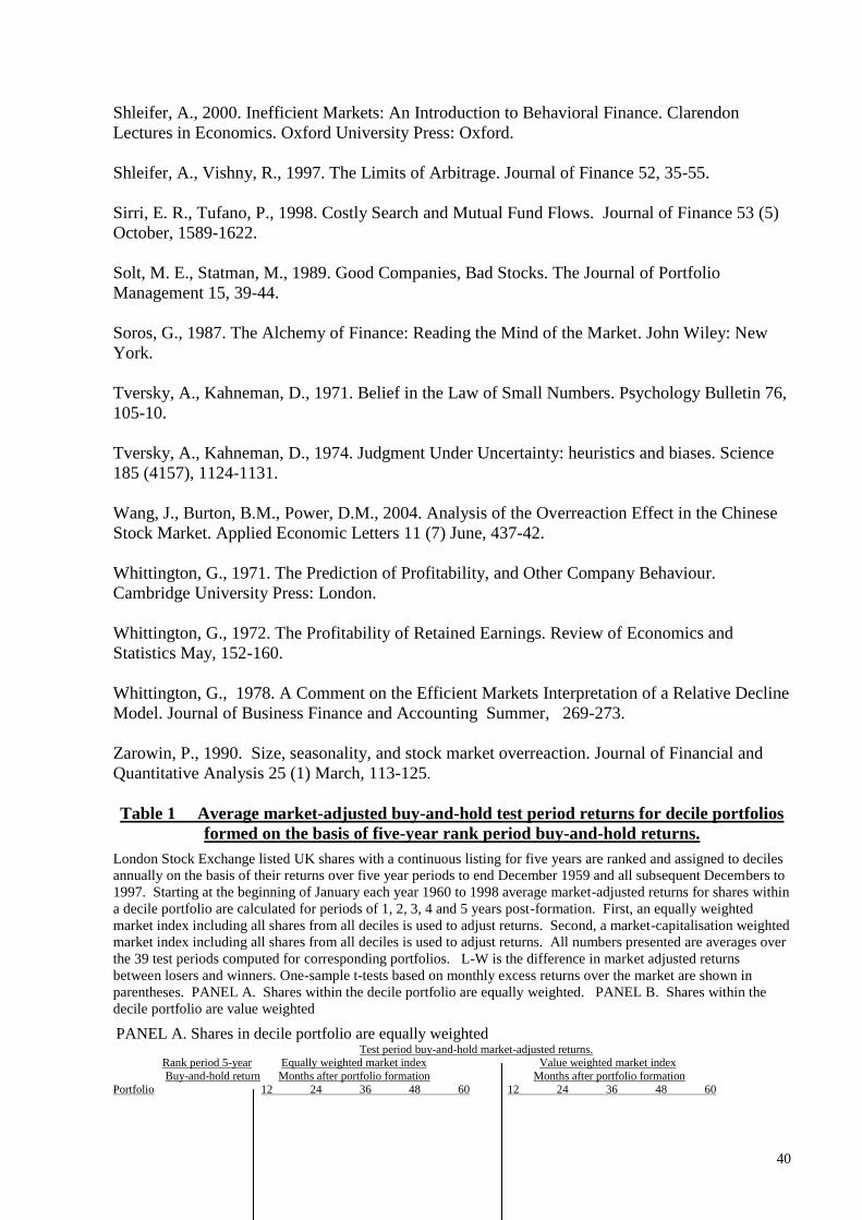
40
Shleifer, A., 2000. Inefficient Markets: An Introduction to Behavioral Finance. Clarendon
Lectures in Economics. Oxford University Press: Oxford.
Shleifer, A., Vishny, R., 1997. The Limits of Arbitrage. Journal of Finance 52, 35-55.
Sirri, E. R., Tufano, P., 1998. Costly Search and Mutual Fund Flows. Journal of Finance 53 (5)
October, 1589-1622.
Solt, M. E., Statman, M., 1989. Good Companies, Bad Stocks. The Journal of Portfolio
Management 15, 39-44.
Soros, G., 1987. The Alchemy of Finance: Reading the Mind of the Market. John Wiley: New
York.
Tversky, A., Kahneman, D., 1971. Belief in the Law of Small Numbers. Psychology Bulletin 76,
105-10.
Tversky, A., Kahneman, D., 1974. Judgment Under Uncertainty: heuristics and biases. Science
185 (4157), 1124-1131.
Wang, J., Burton, B.M., Power, D.M., 2004. Analysis of the Overreaction Effect in the Chinese
Stock Market. Applied Economic Letters 11 (7) June, 437-42.
Whittington, G., 1971. The Prediction of Profitability, and Other Company Behaviour.
Cambridge University Press: London.
Whittington, G., 1972. The Profitability of Retained Earnings. Review of Economics and
Statistics May, 152-160.
Whittington, G., 1978. A Comment on the Efficient Markets Interpretation of a Relative Decline
Model. Journal of Business Finance and Accounting Summer, 269-273.
Zarowin, P., 1990. Size, seasonality, and stock market overreaction. Journal of Financial and
Quantitative Analysis 25 (1) March, 113-125.
Table 1 Average market-adjusted buy-and-hold test period returns for decile portfolios
formed on the basis of five-year rank period buy-and-hold returns.
London Stock Exchange listed UK shares with a continuous listing for five years are ranked and assigned to deciles
annually on the basis of their returns over five year periods to end December 1959 and all subsequent Decembers to
1997. Starting at the beginning of January each year 1960 to 1998 average market-adjusted returns for shares within
a decile portfolio are calculated for periods of 1, 2, 3, 4 and 5 years post-formation. First, an equally weighted
market index including all shares from all deciles is used to adjust returns. Second, a market-capitalisation weighted
market index including all shares from all deciles is used to adjust returns. All numbers presented are averages over
the 39 test periods computed for corresponding portfolios. L-W is the difference in market adjusted returns
between losers and winners. One-sample t-tests based on monthly excess returns over the market are shown in
parentheses. PANEL A. Shares within the decile portfolio are equally weighted. PANEL B. Shares within the
decile portfolio are value weighted
PANEL A. Shares in decile portfolio are equally weighted Test period buy-and-hold market-adjusted returns. Rank period 5-year Equally weighted market index Value weighted market index
Buy-and-hold return Months after portfolio formation Months after portfolio formation
Portfolio 12 24 36 48 60 12 24 36 48 60
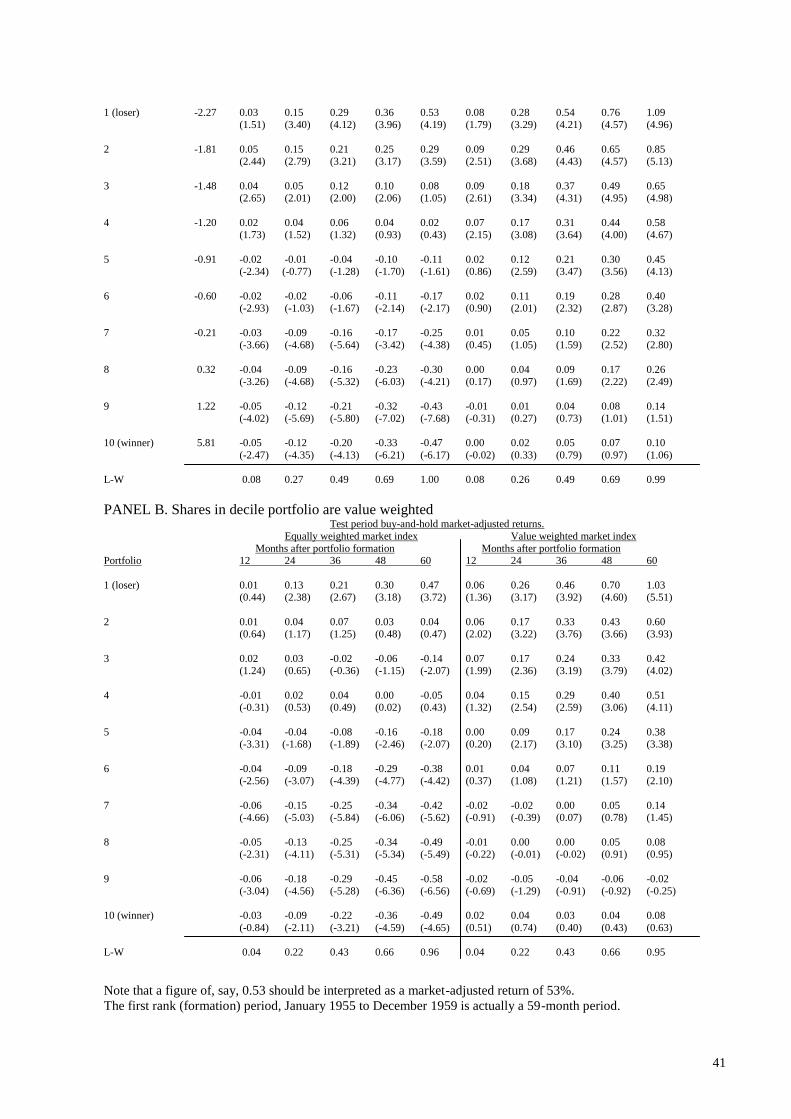
41
1 (loser) -2.27 0.03 0.15 0.29 0.36 0.53 0.08 0.28 0.54 0.76 1.09
(1.51) (3.40) (4.12) (3.96) (4.19) (1.79) (3.29) (4.21) (4.57) (4.96)
2 -1.81 0.05 0.15 0.21 0.25 0.29 0.09 0.29 0.46 0.65 0.85 (2.44) (2.79) (3.21) (3.17) (3.59) (2.51) (3.68) (4.43) (4.57) (5.13)
3 -1.48 0.04 0.05 0.12 0.10 0.08 0.09 0.18 0.37 0.49 0.65 (2.65) (2.01) (2.00) (2.06) (1.05) (2.61) (3.34) (4.31) (4.95) (4.98)
4 -1.20 0.02 0.04 0.06 0.04 0.02 0.07 0.17 0.31 0.44 0.58 (1.73) (1.52) (1.32) (0.93) (0.43) (2.15) (3.08) (3.64) (4.00) (4.67)
5 -0.91 -0.02 -0.01 -0.04 -0.10 -0.11 0.02 0.12 0.21 0.30 0.45 (-2.34) (-0.77) (-1.28) (-1.70) (-1.61) (0.86) (2.59) (3.47) (3.56) (4.13)
6 -0.60 -0.02 -0.02 -0.06 -0.11 -0.17 0.02 0.11 0.19 0.28 0.40 (-2.93) (-1.03) (-1.67) (-2.14) (-2.17) (0.90) (2.01) (2.32) (2.87) (3.28)
7 -0.21 -0.03 -0.09 -0.16 -0.17 -0.25 0.01 0.05 0.10 0.22 0.32 (-3.66) (-4.68) (-5.64) (-3.42) (-4.38) (0.45) (1.05) (1.59) (2.52) (2.80)
8 0.32 -0.04 -0.09 -0.16 -0.23 -0.30 0.00 0.04 0.09 0.17 0.26
(-3.26) (-4.68) (-5.32) (-6.03) (-4.21) (0.17) (0.97) (1.69) (2.22) (2.49)
9 1.22 -0.05 -0.12 -0.21 -0.32 -0.43 -0.01 0.01 0.04 0.08 0.14 (-4.02) (-5.69) (-5.80) (-7.02) (-7.68) (-0.31) (0.27) (0.73) (1.01) (1.51)
10 (winner) 5.81 -0.05 -0.12 -0.20 -0.33 -0.47 0.00 0.02 0.05 0.07 0.10
(-2.47) (-4.35) (-4.13) (-6.21) (-6.17) (-0.02) (0.33) (0.79) (0.97) (1.06)
L-W 0.08 0.27 0.49 0.69 1.00 0.08 0.26 0.49 0.69 0.99
PANEL B. Shares in decile portfolio are value weighted Test period buy-and-hold market-adjusted returns.
Equally weighted market index Value weighted market index
Months after portfolio formation Months after portfolio formation Portfolio 12 24 36 48 60 12 24 36 48 60
1 (loser) 0.01 0.13 0.21 0.30 0.47 0.06 0.26 0.46 0.70 1.03 (0.44) (2.38) (2.67) (3.18) (3.72) (1.36) (3.17) (3.92) (4.60) (5.51)
2 0.01 0.04 0.07 0.03 0.04 0.06 0.17 0.33 0.43 0.60
(0.64) (1.17) (1.25) (0.48) (0.47) (2.02) (3.22) (3.76) (3.66) (3.93)
3 0.02 0.03 -0.02 -0.06 -0.14 0.07 0.17 0.24 0.33 0.42 (1.24) (0.65) (-0.36) (-1.15) (-2.07) (1.99) (2.36) (3.19) (3.79) (4.02)
4 -0.01 0.02 0.04 0.00 -0.05 0.04 0.15 0.29 0.40 0.51 (-0.31) (0.53) (0.49) (0.02) (0.43) (1.32) (2.54) (2.59) (3.06) (4.11)
5 -0.04 -0.04 -0.08 -0.16 -0.18 0.00 0.09 0.17 0.24 0.38 (-3.31) (-1.68) (-1.89) (-2.46) (-2.07) (0.20) (2.17) (3.10) (3.25) (3.38)
6 -0.04 -0.09 -0.18 -0.29 -0.38 0.01 0.04 0.07 0.11 0.19 (-2.56) (-3.07) (-4.39) (-4.77) (-4.42) (0.37) (1.08) (1.21) (1.57) (2.10)
7 -0.06 -0.15 -0.25 -0.34 -0.42 -0.02 -0.02 0.00 0.05 0.14 (-4.66) (-5.03) (-5.84) (-6.06) (-5.62) (-0.91) (-0.39) (0.07) (0.78) (1.45)
8 -0.05 -0.13 -0.25 -0.34 -0.49 -0.01 0.00 0.00 0.05 0.08 (-2.31) (-4.11) (-5.31) (-5.34) (-5.49) (-0.22) (-0.01) (-0.02) (0.91) (0.95)
9 -0.06 -0.18 -0.29 -0.45 -0.58 -0.02 -0.05 -0.04 -0.06 -0.02 (-3.04) (-4.56) (-5.28) (-6.36) (-6.56) (-0.69) (-1.29) (-0.91) (-0.92) (-0.25)
10 (winner) -0.03 -0.09 -0.22 -0.36 -0.49 0.02 0.04 0.03 0.04 0.08
(-0.84) (-2.11) (-3.21) (-4.59) (-4.65) (0.51) (0.74) (0.40) (0.43) (0.63)
L-W 0.04 0.22 0.43 0.66 0.96 0.04 0.22 0.43 0.66 0.95
Note that a figure of, say, 0.53 should be interpreted as a market-adjusted return of 53%.
The first rank (formation) period, January 1955 to December 1959 is actually a 59-month period.

42
Table 2 Large capitalization company analysis.
Average market-adjusted buy-and-hold test period returns for decile portfolios formed on
the basis of five-year rank period buy-and-hold returns.
The largest 20% of firms in the sample with a continuous listing for five years are ranked and assigned to deciles
annually on the basis of their returns over five year periods to end December 1959 and all subsequent Decembers to
1997. At the beginning of January each year 1960 to 1998 average market-adjusted returns for shares within a
decile portfolio are calculated for periods of 1, 2, 3, 4 and 5 years post-formation. First, an equally weighted market
index including all shares (as in table 1) is used to adjust returns. Second, a market-capitalisation weighted market
index (as in table 1) is used to adjust returns. The market indices are constructed using all the companies in the
sample, not just the largest 20 per cent. All numbers presented are averages over the 39 rank periods computed for
corresponding portfolios. L-W is the difference in market-adjusted returns between losers and winners. One-
sample t-tests based on monthly excess returns over the market are shown in parentheses. PANEL A. Shares within
the decile portfolio are equally weighted. PANEL B. Shares within the decile portfolio are value weighted
PANEL A. Shares in decile portfolio are equally weighted
Test period buy-and-hold market-adjusted returns.
Rank period 5-year Equally weighted market index Value weighted market index
buy-and-hold return Months after portfolio formation Months after portfolio formation Portfolio 12 24 36 48 60 12 24 36 48 60
1 (loser) -0.30 -0.02 0.01 0.02 -0.02 0.04 0.02 0.15 0.27 0.38 0.61
(-0.69) (0.21) (0.28) (-0.18) (0.28) (0.62) (2.30) (3.02) (3.20) (3.22)
2 0.19 0.00 0.02 0.11 0.10 0.10 0.04 0.15 0.36 0.50 0.66
(-0.03) (0.33) (0.65) (0.65) (0.57) (1.34) (2.65) (2.05) (2.52) (2.88)
3 0.50 -0.01 -0.06 -0.14 -0.17 -0.18 0.03 0.07 0.11 0.23 0.38
(-0.31) (-1.16) (-2.30) (-2.31) (-1.51) (0.96) (1.60) (1.80) (3.06) (3.17)
4 0.70 -0.01 -0.06 -0.09 -0.17 -0.21 0.04 0.07 0.16 0.23 0.35
(-0.33) (-1.11) (-0.97) (-1.49) (-1.59) (1.39) (1.63) (1.71) (1.82) (2.57)
5 0.91 -0.03 -0.07 -0.17 -0.28 -0.38 0.01 0.06 0.08 0.11 0.18
(-1.22) (-1.54) (-3.04) (-3.22) (-3.15) (0.68) (1.66) (1.40) (1.52) (1.55)
6 1.14 -0.06 -0.13 -0.19 -0.35 -0.49 -0.01 0.00 0.06 0.05 0.07
(-2.12) (-2.72) (-2.86) (-3.86) (-5.16) (-0.70) (0.16) (1.19) (0.67) (0.88)
7 1.40 -0.05 -0.12 -0.21 -0.29 -0.36 -0.01 0.02 0.04 0.11 0.20
(-2.02) (-1.84) (-3.19) (-3.42) (-2.98) (-0.43) (0.30) (0.64) (1.37) (1.87)
8 1.73 -0.04 -0.15 -0.26 -0.38 -0.56 0.00 -0.02 0.00 0.02 0.00
(-1.79) (-3.63) (-3.71) (-3.17) (-3.79) (0.01) (-0.54) (-0.08) (0.23) (0.05)
9 2.27 -0.08 -0.20 -0.35 -0.56 -0.75 -0.04 -0.07 -0.09 -0.16 -0.19
(-2.70) (-3.94) (-5.21) (-6.60) (-6.40) (-2.23) (-2.11) (-2.62) (-3.56) (-3.37)

43
10 (winner) 3.91 -0.05 -0.15 -0.30 -0.47 -0.67 -0.01 -0.02 -0.05 -0.07 -0.11
(-1.88) (-2.66) (-3.40) (-3.74) (-4.30) (-0.37) (-0.50) (-1.01) (-1.01) (-1.19)
L-W 0.03 0.16 0.32 0.45 0.71 0.03 0.17 0.32 0.45 0.72
Table 2 (continued)
PANEL B. Shares in decile portfolio are value weighted
Test period buy-and-hold market-adjusted returns.
Equally weighted market index Value weighted market index
Months after portfolio formation Months after portfolio formation Portfolio 12 24 36 48 60 12 24 36 48 60
1 (loser) 0.02 0.07 0.14 0.15 0.33 0.06 0.20 0.39 0.54 0.89
(0.44) (0.82) (1.09) (1.06) (1.80) (1.81) (2.68) (3.21) (3.78) (4.13)
2 0.01 0.04 0.02 0.01 0.02 0.05 0.17 0.28 0.41 0.58
(0.27) (0.66) (0.26) (0.10) (0.13) (1.47) (2.83) (2.97) (3.07) (3.62)
3 -0.03 -0.08 -0.20 -0.17 -0.15 0.02 0.06 0.06 0.23 0.42
(-1.08) (-1.43) (-3.11) (-1.56) (-0.86) (0.85) (1.40) (1.03) (2.16) (2.42)
4 -0.00 -0.03 -0.08 -0.21 -0.28 0.05 0.11 0.17 0.18 0.29
(0.13) (-0.42) (-0.84) (-2.06) (-2.38) (1.71) (2.08) (1.84) (1.60) (2.26)
5 -0.02 -0.05 -0.16 -0.29 -0.40 0.03 0.08 0.10 0.10 0.17
(-0.68) (-1.25) (-2.85) (-3.32) (-3.08) (1.18) (2.12) (1.84) (1.38) (1.40)
6 -0.07 -0.16 -0.25 -0.39 -0.53 -0.02 -0.03 0.00 0.01 0.03
(-2.57) (-3.16) (-3.63) (-4.65) (-5.31) (-1.31) (-0.77) (0.09) (0.17) (0.37)
7 -0.07 -0.15 -0.25 -0.32 -0.42 -0.02 -0.02 0.00 0.07 0.14
(-2.33) (-2.85) (-3.72) (-3.43) (-2.93) (-1.15) (-0.49) (0.02) (1.01) (1.25)
8 -0.04 -0.15 -0.25 -0.36 -0.58 0.00 -0.01 0.00 0.04 -0.01
(-1.44) (-3.23) (-3.37) (-2.83) (-3.71) (0.19) (-0.45) (-0.01) (0.37) (-0.12)
9 -0.07 -0.17 -0.36 -0.56 -0.77 -0.03 -0.04 -0.10 -0.16 -0.20
(-1.73) (-2.59) (-4.64) (-5.31) (-5.66) (-0.87) (-0.72) (-2.18) (-2.68) (-2.88)
10 (winner) -0.04 -0.16 -0.30 -0.46 -0.59 0.01 -0.03 -0.05 -0.07 -0.03
(-1.19) (-2.43) (-3.24) (-3.45) (-3.35) (0.25) (-0.65) (-0.92) (-0.79) (-0.24)
L-W 0.06 0.23 0.44 0.61 0.92 0.05 0.23 0.44 0.61 0.92
Note that a figure of, say, -0.02 should be interpreted as a market-adjusted return of -2%.

44
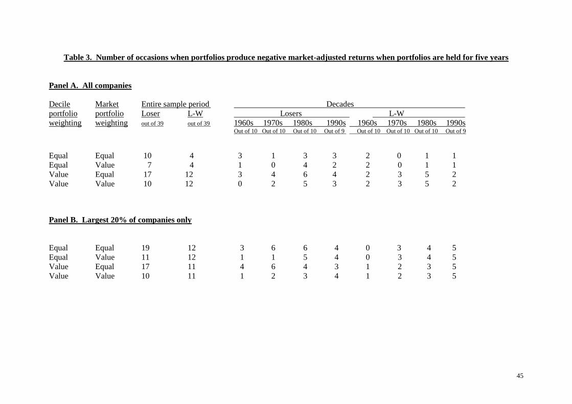
45
Table 3. Number of occasions when portfolios produce negative market-adjusted returns when portfolios are held for five years
Panel A. All companies
Decile Market Entire sample period Decades
portfolio portfolio Loser L-W Losers L-W
weighting weighting out of 39 out of 39 1960s 1970s 1980s 1990s 1960s 1970s 1980s 1990s Out of 10 Out of 10 Out of 10 Out of 9 Out of 10 Out of 10 Out of 10 Out of 9
Equal Equal 10 4 3 1 3 3 2 0 1 1
Equal Value 7 4 1 0 4 2 2 0 1 1
Value Equal 17 12 3 4 6 4 2 3 5 2
Value Value 10 12 0 2 5 3 2 3 5 2
Panel B. Largest 20% of companies only
Equal Equal 19 12 3 6 6 4 0 3 4 5
Equal Value 11 12 1 1 5 4 0 3 4 5
Value Equal 17 11 4 6 4 3 1 2 3 5
Value Value 10 11 1 2 3 4 1 2 3 5

46
Table 4
Average number of shares in each portfolio during the test period and number of
companies deleted in the test period – full sample.
PANEL A: The number of shares remaining in each portfolio after 1, 2, 3, 4 and 5 years
averaged for the 39 portfolio formations
Months after formation
0 12 24 36 48 60
Portfolio
1 (loser) 95.6 86.4 79.0 72.0 65.8 59.9
2 95.7 95.6 81.5 75.6 70.1 64.4
3 95.8 95.7 84.2 78.9 73.7 68.4
4 95.9 95.7 84.0 78.3 73.8 69.4
5 96.0 95.9 85.0 79.9 74.5 69.8
6 96.2 96.1 85.6 80.6 75.2 70.6
7 96.3 96.1 86.5 81.7 77.0 72.7
8 96.4 96.2 86.8 82.1 77.2 72.8
9 96.5 96.3 86.4 82.0 77.5 73.8
10 (winner) 96.6 96.4 87.0 81.6 76.7 71.7
PANEL B Number of companies deleted (cumulative) due to mergers, liquidations and other
reasons Li = number of companies deleted due to liquidation, M = number of companies deleted due to being acquired in
merger/takeover, O = number of companies deleted due to other reasons.
Months after
formation
12
24
36
48
60
Portfolio M Li O M Li O M Li O M Li O M Li O
1 (L) 5.0 3.7 0.4 9.5 6.1 1.1 14.1 8.0 1.6 18.2 9.6 2.1 21.9 11.3 2.6
2 5.7 1.0 0.4 11.3 2.2 0.7 16.0 3.4 0.9 20.0 4.5 1.3 24.2 5.5 1.6
3 4.6 0.6 0.3 9.4 1.7 0.5 14.1 2.3 0.7 18.5 2.8 1.0 22.3 3.8 1.3
4 4.9 0.5 0.3 10.1 1.3 0.6 15.0 1.8 0.9 18.7 2.4 1.3 22.2 2.8 1.5
5 4.8 0.5 0.1 9.7 0.9 0.4 14.2 1.5 0.6 18.7 2.0 0.8 22.4 2.6 1.1
6 4.8 0.4 0.1 9.7 0.7 0.2 14.1 1.3 0.4 18.8 1.8 0.5 22.4 2.3 0.8
7 4.5 0.3 0.2 8.7 0.7 0.4 12.9 1.2 0.6 16.8 1.8 0.8 20.3 2.3 0.9
8 4.0 0.2 0.3 8.4 0.7 0.5 12.5 1.1 0.8 16.6 1.6 1.0 20.5 1.9 1.1
9 4.3 0.2 0.3 8.7 0.7 0.7 12.3 1.2 1.1 15.9 1.7 1.4 18.9 2.0 1.7
10 (W) 3.8 0.5 0.4 7.6 1.1 0.9 12.0 1.8 1.4 16.0 2.4 1.8 19.9 2.9 2.1
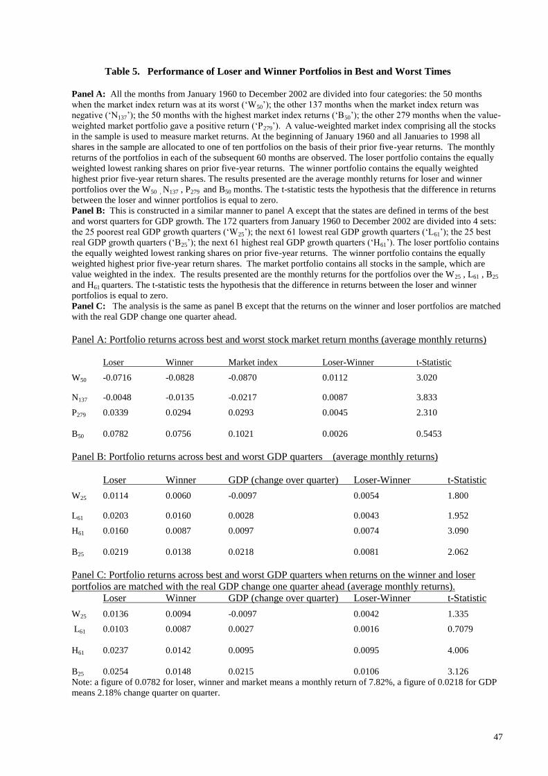
47
Table 5. Performance of Loser and Winner Portfolios in Best and Worst Times
Panel A: All the months from January 1960 to December 2002 are divided into four categories: the 50 months
when the market index return was at its worst („W50‟); the other 137 months when the market index return was
negative („N137‟); the 50 months with the highest market index returns („B50‟); the other 279 months when the value-
weighted market portfolio gave a positive return („P279‟). A value-weighted market index comprising all the stocks
in the sample is used to measure market returns. At the beginning of January 1960 and all Januaries to 1998 all
shares in the sample are allocated to one of ten portfolios on the basis of their prior five-year returns. The monthly
returns of the portfolios in each of the subsequent 60 months are observed. The loser portfolio contains the equally
weighted lowest ranking shares on prior five-year returns. The winner portfolio contains the equally weighted
highest prior five-year return shares. The results presented are the average monthly returns for loser and winner
portfolios over the W50 , N137 , P279 and B50 months. The t-statistic tests the hypothesis that the difference in returns
between the loser and winner portfolios is equal to zero.
Panel B: This is constructed in a similar manner to panel A except that the states are defined in terms of the best
and worst quarters for GDP growth. The 172 quarters from January 1960 to December 2002 are divided into 4 sets:
the 25 poorest real GDP growth quarters („W25‟); the next 61 lowest real GDP growth quarters („L61‟); the 25 best
real GDP growth quarters („B25‟); the next 61 highest real GDP growth quarters („H61‟). The loser portfolio contains
the equally weighted lowest ranking shares on prior five-year returns. The winner portfolio contains the equally
weighted highest prior five-year return shares. The market portfolio contains all stocks in the sample, which are
value weighted in the index. The results presented are the monthly returns for the portfolios over the W25 , L61 , B25
and H61 quarters. The t-statistic tests the hypothesis that the difference in returns between the loser and winner
portfolios is equal to zero.
Panel C: The analysis is the same as panel B except that the returns on the winner and loser portfolios are matched
with the real GDP change one quarter ahead.
Panel A: Portfolio returns across best and worst stock market return months (average monthly returns)
Loser Winner Market index Loser-Winner t-Statistic
W50 -0.0716 -0.0828 -0.0870 0.0112 3.020
N137 -0.0048 -0.0135 -0.0217 0.0087 3.833
P279 0.0339 0.0294 0.0293 0.0045 2.310
B50 0.0782 0.0756 0.1021 0.0026 0.5453
Panel B: Portfolio returns across best and worst GDP quarters (average monthly returns)
Loser Winner GDP (change over quarter) Loser-Winner t-Statistic
W25 0.0114 0.0060 -0.0097 0.0054 1.800
L61 0.0203 0.0160 0.0028 0.0043 1.952
H61 0.0160 0.0087 0.0097 0.0074 3.090
B25 0.0219 0.0138 0.0218 0.0081 2.062
Panel C: Portfolio returns across best and worst GDP quarters when returns on the winner and loser
portfolios are matched with the real GDP change one quarter ahead (average monthly returns).
Loser Winner GDP (change over quarter) Loser-Winner t-Statistic
W25 0.0136 0.0094 -0.0097 0.0042 1.335
L61 0.0103 0.0087 0.0027 0.0016 0.7079
H61 0.0237 0.0142 0.0095 0.0095 4.006
B25 0.0254 0.0148 0.0215 0.0106 3.126
Note: a figure of 0.0782 for loser, winner and market means a monthly return of 7.82%, a figure of 0.0218 for GDP
means 2.18% change quarter on quarter.

48
Table 6 Beta and Standard Deviation for Portfolios All LSE UK listed shares are ranked and allocated to rank period return deciles each January from 1960 to 1998.
For the first test period year following portfolio formation we observe the raw returns of the portfolio relative to the
Treasury Bill rate and the return on a value-weighted market portfolio relative to the Treasury Bill rate. The
regressions are based on all the annual observations for a portfolio, drawing on all 39 portfolio formations. The
analysis is repeated for each of the test years. Using the 39 formation periods, we also compute the standard
deviation of returns in the year after formation and in each of the other test years. An arbitrage portfolio (L-W) is
constructed by subtracting the test period annual return for the winner portfolio from the return on the loser portfolio
for that year.
rpt - rft = αp + βp (rmt – rft) + ℮t rLt - rWt = αL-W + βL-W (rmt – rft) + ℮t
Test year Decile Alpha Beta Standard deviation
after formation 1 1 (Loser) 0.0479 1.1196 0.2107 1 2 0.0505 1.2780 0.1799
1 3 0.0335 1.2521 0.1754
1 4 0.0348 1.2056 0.1627 1 5 0.0078 1.1827 0.1374
1 6 0.0019 1.1984 0.1384
1 7 -0.0013 1.1461 0.1305
1 8 0.0034 1.0396 0.1307
1 9 -0.0128 1.1110 0.1414
1 10 (Winner) -0.0114 1.1599 0.1433 1 L-W 0.0593 -0.0403 0.1555
2 1 (loser) 0.0953 1.0990 0.2339 2 2 0.0732 1.3719 0.1738
2 3 0.0444 1.1259 0.1418
2 4 0.0393 1.1090 0.1469 2 5 0.0490 1.1329 0.1490
2 6 0.0439 1.0556 0.1469
2 7 0.0024 1.1419 0.1441 2 8 0.0089 1.1094 0.1488
2 9 -0.0062 1.1922 0.1328
2 10 (Winner) -0.0219 1.1739 0.1866 2 L-W 0.1172 -0.0749 0.1812
3 1 (Loser) 0.0695 1.1478 0.2258
3 2 0.0430 1.0277 0.2094
3 3 0.0470 1.3087 0.1772 3 4 0.0377 1.0468 0.1506
3 5 0.0163 1.2381 0.1369
3 6 0.0125 1.1295 0.1433 3 7 0.0068 1.1567 0.1291
3 8 0.0082 1.1093 0.1494
3 9 -0.0010 1.1003 0.1415 3 10 (Winner) -0.0170 1.2897 0.1783
3 L-W 0.0865 -0.1418 0.1808
4 1 (Loser) 0.0498 1.0861 0.2085
4 2 0.0373 1.0807 0.1923
4 3 0.0266 0.9741 0.1866 4 4 0.0205 1.1246 0.1426
4 5 0.0017 1.2070 0.1597
4 6 0.0172 1.1809 0.1358 4 7 0.0328 1.1838 0.1744
4 8 0.0237 1.1267 0.1532
4 9 -0.0015 1.1744 0.1363 4 10 (Winner) -0.0098 1.1439 0.1639
4 L-W 0.0597 -0.0578 0.1312
5 1 (Loser) 0.0565 1.0910 0.1916
5 2 0.0413 1.1491 0.1717
5 3 0.0427 1.0195 0.1798 5 4 0.0280 1.0721 0.1593
5 5 0.0276 1.1403 0.1511
5 6 0.0225 1.0661 0.1377 5 7 0.0235 0.9388 0.1596
5 8 0.0217 1.1604 0.1605
5 9 0.0241 1.0995 0.1482 5 10 (Winner) 0.0045 1.0471 0.1604
5 L-W 0.0520 0.0439 0.1371
An alpha return of 0.0479 should be interpreted as 4.79% per year


50
Table 7 Three factor time series regressions for portfolios All LSE UK listed shares are ranked and allocated to rank period return deciles each January from 1960 to 1998. For the first test period year following portfolio formation
we observe the value-weighted returns of the portfolio relative to the Treasury Bill rate and the return on a value-weighted market portfolio relative to the Treasury Bill rate.
The difference in monthly return between small market capitalization firms and large firms (SMB) is taken from Dimson, Nagel and Quigley (2003) based on the method of
Fama and French (1993, 1996). The difference in monthly return for high book-to-market ratio companies and low book-to-market ratio companies (HML) is taken from
Dimson, Nagel and Quigley (2003). The regressions are based on all the monthly observations for a portfolio, drawing on all 39 portfolio formations. For the remaining four
regressions (for post-formation years 2 to 5), we regress monthly excess returns on the portfolio in the year on the contemporaneous excess return on the market factor and on
the HML and SMB factors created in the first test period year. An arbitrage portfolio (L-W) is constructed by subtracting the test period monthly return for the winner
portfolio from the return on the loser portfolio for that month.
rp – rf = p + bp (rm – rf) + sp(SMB) + hp(HML) + p
year 1-5 decile alpha se p-value bp sp hp sigma Rsq 1 1 (Loser) 0.0005 0.0016 0.381004 1.1460 1.0690 0.6407 0.0333 0.74
1 2 0.0034 0.0011 0.001146 1.0056 0.7330 0.3882 0.0229 0.82
1 9 -0.0005 0.0008 0.755975 0.9499 0.6741 -0.0151 0.0163 0.89
1 10(Winner) 0.0001 0.0010 0.473967 0.9519 0.6943 -0.0771 0.0199 0.84
1 L-W 0.0004 0.0019 0.411228 0.1941 0.3748 0.7179 0.0392 0.17
2 1(Loser) 0.0088 0.0021 0.000018 0.7757 0.0345 0.0915 0.0441 0.47
2 2 0.0087 0.0018 0.000001 0.8127 0.0915 -0.0528 0.0380 0.57
2 9 0.0013 0.0012 0.142589 0.7975 -0.0238 -0.0394 0.0255 0.74
2 10(Winner) 0.0002 0.0014 0.444854 0.8006 0.0334 -0.1116 0.0300 0.67
2 L-W 0.0086 0.0019 0.000004 -0.0249 0.0011 0.2031 0.0399 0.01
3 1(Loser) 0.0074 0.0021 0.000266 0.7474 0.0159 0.0729 0.0444 0.45
3 2 0.0041 0.0019 0.016055 0.7860 -0.0508 0.1640 0.0395 0.54
3 9 0.0020 0.0015 0.086217 0.7659 0.0116 -0.0917 0.0303 0.65
3 10(Winner) 0.0010 0.0015 0.266894 0.8726 0.0593 -0.0779 0.0323 0.68
3 L-W 0.0065 0.0018 0.000261 -0.1253 -0.0434 0.1508 0.0386 0.03
4 1(Loser) 0.0052 0.0020 0.005514 0.7620 -0.1039 0.0899 0.0424 0.49
4 2 0.0045 0.0017 0.004460 0.7518 -0.0741 -0.0002 0.0362 0.56
4 9 0.0014 0.0013 0.146630 0.8283 -0.0754 -0.0040 0.0277 0.72
4 10(Winner) -0.0004 0.0017 0.590565 0.8726 -0.0248 0.1580 0.0352 0.65
4 L-W 0.0056 0.0019 0.001934 -0.1106 -0.0791 -0.0681 0.0400 0.03
5 1(Loser) 0.0049 0.0021 0.008962 0.7732 -0.0420 0.2192 0.0431 0.49
5 2 0.0048 0.0017 0.003201 0.7679 -0.0180 0.0157 0.0364 0.57
5 9 0.0032 0.0014 0.009226 0.8176 -0.0066 -0.0388 0.0287 0.71
5 10(Winner) 0.0010 0.0018 0.293463 0.8714 -0.0146 0.0255 0.0368 0.63
5 L-W 0.0039 0.0019 0.019516 -0.0982 -0.0274 0.1936 0.0398 0.03
An alpha return of 0.0049 should be interpreted as 0.49% per month

51
Table 8
Percentage of firms within each size decile falling in each rank period return decile At each formation date, 1960-98, all LSE listed UK shares in the sample are sorted according to size and
allocated to one of ten portfolios. Shares are also sorted on the basis of the rank period buy-and-hold returns.
The numbers shown are the percentage of each size-based decile independently allocated to each rank period
buy-and-hold return decile when the 39 test periods are aggregated.
Size Decile
Deciles 1 2 3 4 5 6 7 8 9 10
defined by
rank period
returns
1 24.5 15.4 10.8 9.0 8.3 6.3 6.6 6.6 6.3 6.3
2 16.7 13.5 12.1 9.9 8.8 8.7 8.5 7.9 7.1 6.9
3 14.2 12.4 10.9 10.5 9.6 8.6 8.9 8.2 8.6 8.2
4 10.5 10.6 11.0 10.4 9.6 9.2 9.4 9.8 9.5 9.8
5 9.6 10.6 9.7 9.2 10.5 10.2 9.5 9.3 10.0 11.6
6 7.6 8.3 10.2 9.8 9.3 11.1 9.4 11.0 11.1 12.3
7 5.2 8.0 8.5 10.7 10.2 10.3 10.8 11.0 12.0 13.4
8 5.1 7.9 8.9 9.7 9.4 11.4 11.1 12.0 11.7 12.7
9 4.1 6.8 8.9 9.2 11.0 11.0 12.4 11.8 13.2 11.6
10 2.3 6.3 8.6 11.4 13.3 13.4 13.5 12.7 10.9 7.6
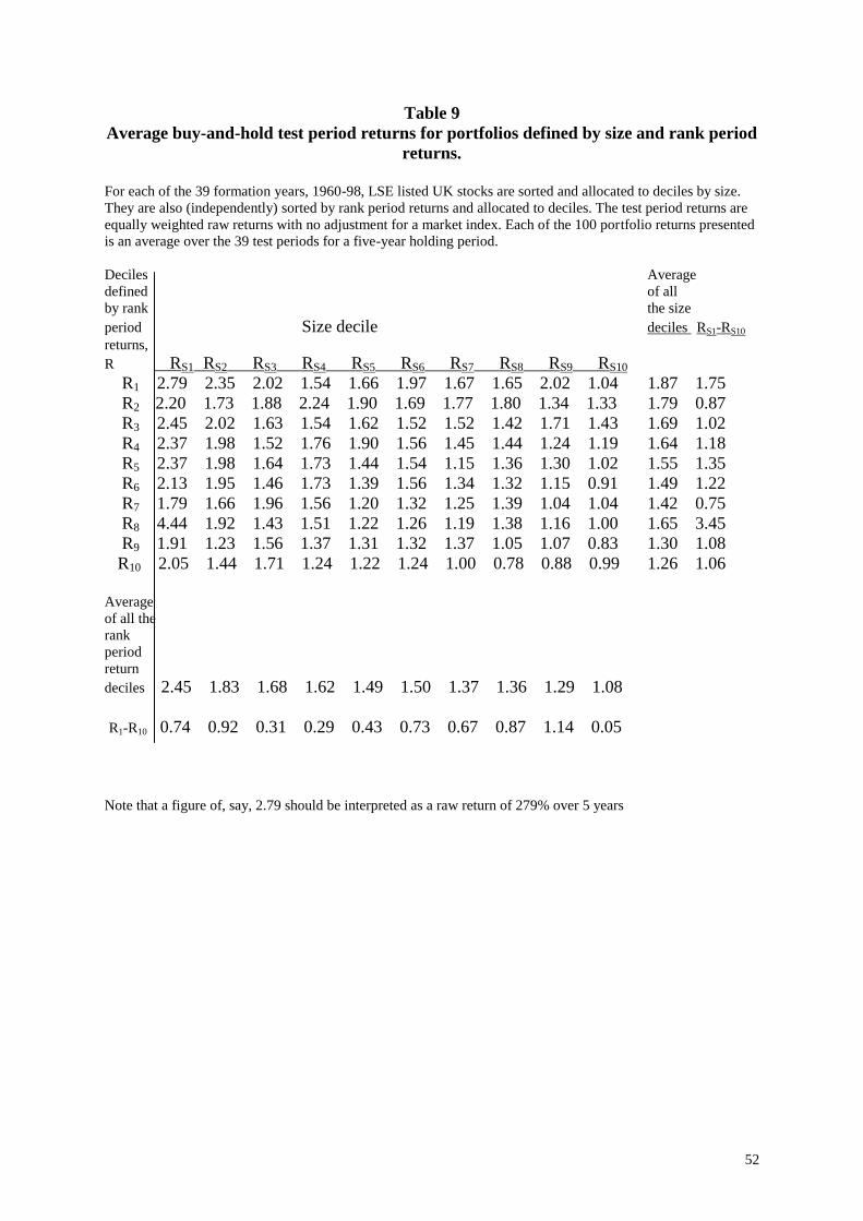
52
Table 9
Average buy-and-hold test period returns for portfolios defined by size and rank period
returns.
For each of the 39 formation years, 1960-98, LSE listed UK stocks are sorted and allocated to deciles by size.
They are also (independently) sorted by rank period returns and allocated to deciles. The test period returns are
equally weighted raw returns with no adjustment for a market index. Each of the 100 portfolio returns presented
is an average over the 39 test periods for a five-year holding period.
Deciles Average
defined of all
by rank the size
period Size decile deciles RS1-RS10
returns,
R RS1 RS2 RS3 RS4 RS5 RS6 RS7 RS8 RS9 RS10
R1 2.79 2.35 2.02 1.54 1.66 1.97 1.67 1.65 2.02 1.04 1.87 1.75
R2 2.20 1.73 1.88 2.24 1.90 1.69 1.77 1.80 1.34 1.33 1.79 0.87
R3 2.45 2.02 1.63 1.54 1.62 1.52 1.52 1.42 1.71 1.43 1.69 1.02
R4 2.37 1.98 1.52 1.76 1.90 1.56 1.45 1.44 1.24 1.19 1.64 1.18
R5 2.37 1.98 1.64 1.73 1.44 1.54 1.15 1.36 1.30 1.02 1.55 1.35
R6 2.13 1.95 1.46 1.73 1.39 1.56 1.34 1.32 1.15 0.91 1.49 1.22
R7 1.79 1.66 1.96 1.56 1.20 1.32 1.25 1.39 1.04 1.04 1.42 0.75
R8 4.44 1.92 1.43 1.51 1.22 1.26 1.19 1.38 1.16 1.00 1.65 3.45
R9 1.91 1.23 1.56 1.37 1.31 1.32 1.37 1.05 1.07 0.83 1.30 1.08
R10 2.05 1.44 1.71 1.24 1.22 1.24 1.00 0.78 0.88 0.99 1.26 1.06
Average of all the
rank
period
return
deciles 2.45 1.83 1.68 1.62 1.49 1.50 1.37 1.36 1.29 1.08
R1-R10 0.74 0.92 0.31 0.29 0.43 0.73 0.67 0.87 1.14 0.05
Note that a figure of, say, 2.79 should be interpreted as a raw return of 279% over 5 years

53
Table 10
Average five-year test period percentage returns for ten portfolios of firms ranked by
their five-year rank period returns, size control portfolios and size-adjusted returns.
For each formation date, 1960-1998, LSE listed UK shares are ranked and allocated to deciles on the basis of
five-year rank period returns. They are also ranked and allocated to deciles by market capitalization. Each share
in a rank period return decile is identified as also belonging to a size decile. The return in the five-year test
period is calculated for each rank period return decile and each size decile (equal weighting of shares within
portfolios). Then size control portfolio returns are calculated by substituting the actual test period return on a
share in a rank period return decile with the return on the size decile that the stock falls into. Size-adjusted
returns are calculated by subtracting the size-control portfolio returns from the actual returns on the rank period
return deciles. This procedure is carried out for each of the portfolio formations and the reported numbers are
averages over the 39 test periods. The tests are 1-sample t-tests, with 38 degrees of freedom. They are based on
the mean return and standard deviation over 39 years (any value whose absolute value exceeds 2.02 makes the t-
test significant at the 5% level).
Five-year test period returns
Portfolio Test period raw Size-control Size-adjusted t-test
returns for portfolios portfolio returns
defined by rank returns
period returns
(Rp) (RS) Rp - RS
1 2.09 1.82 0.28 3.59
2 1.97 1.68 0.28 4.35
3 1.74 1.60 0.14 2.23
4 1.66 1.56 0.10 2.09
5 1.52 1.52 0.00 0.07
6 1.45 1.49 -0.05 -0.83
7 1.39 1.49 -0.10 -2.30
8 1.39 1.50 -0.11 -1.99
9 1.24 1.48 -0.24 -5.41
10 1.18 1.49 -0.31 -4.60
R1 – R10 0.91 0.33 0.58 7.59
Note that a figure of, say, 0.28 in the size-adjusted return column should be interpreted as a 28 % return after
adjustment for size.

54
Fig. 1
Cumulative market-adjusted returns for each decile over a 60 month test period
LSE listed UK stocks are ranked and assigned to deciles annually on the basis of their returns over five year
periods to December 1959 and all subsequent Decembers to 1997. Cumulative equally weighted average
residual returns for stocks month-by-month in the post-formation period are calculated. An equally weighted
market index including all stocks from all deciles is used to adjust returns. All results presented are averages
over the 39 rank periods computed for corresponding portfolios.
Note that a figure of, say, 0.20 should be interpreted as a market-adjusted return of 20%

55
Figure 2. Market-adjusted buy-and-hold five-year test period returns for loser minus
winner strategies for each of the thirty nine portfolio formations.
The five-year test period returns for each loser-winner strategy are assigned to the year of formation.
A year of negative real GDP growth is indicated by and arrow (data sourced from Thompson Datastream)
A year of negative real return on equities is indicated by a square (data sourced from Barclays Capital
Equity Gilt Study 2003)
Figure 2 (a) All sample companies. Loser-winner sixty-month returns. Shares within
decile portfolios equally weighted. Market index constituents equally weighted.
-200
-100
0
100
200
300
400
500
60 62 64 66 68 70 72 74 76 78 80 82 84 86 88 90 92 94 96 98
Year
Perc
en
t re
turn
over
5 y
ears

56
Figure 2 (b) All sample companies. Loser-winner sixty-month returns. Shares within
decile portfolios value weighted. Market index constituents value weighted.
-300
-200
-100
0
100
200
300
400
500
600
700
800
60 62 64 66 68 70 72 74 76 78 80 82 84 86 88 90 92 94 96 98
Year
Perc
en
t re
turn
over
5 y
ears
Figure 2 (c) Largest 20% of companies. Loser-winner sixty-month returns. Shares
within decile portfolios value weighted. Market index constituents value weighted.
-400
-200
0
200
400
600
800
60 62 64 66 68 70 72 74 76 78 80 82 84 86 88 90 92 94 96 98
Year
Perc
en
t re
turn
over
5 y
ears

57
1 For example: Baytas and Cakici (1999) who found return reversal in six countries, Schiereck, De Bondt and
Weber (1999) and Külpman (2002) in German shares, Mun, Vasconcellos and Kish (2000) for Canada and the
US, Da Costa, (1994) for Brazil, Ahmad and Hussain (2001) for Malaysia, Fung (1999) for Hong Kong, Wang
et al. (2004) for Shanghai and Shenzhen. However, Brailsford (1992) failed to find return reversal and Gaunt
(2000) finds only a weak indication of return reversal in the Australian equity market.
2 The LSPD separately provides data on the 500 largest companies in 1955 and the 200 largest companies in
1972. However, to include these in addition to the one-third random sample would bias the results.
3 Earlier studies in this field (e.g De Bondt and Thaler, 1985) are restricted to examining non-overlapping test
periods. However the costs of this approach are loss of information and the possibility that the contrarian
strategy depends upon an economy-wide cyclical factor that coincides with the five-year formation period cycle.
4 All calculations were completed using a purpose-written programme in Fortran 95.
5 The buy-and-hold approach has an advantage over the cumulative abnormal return (CAR) approach because it
reflects a realistic strategy available to a long term investor who would suffer from the high transaction costs
implicitly assumed by the monthly rebalancing in the CAR method. It seems reasonable to judge the success of
the contrarian strategy on the basis of the one-off decision to buy or sell stocks on portfolio formation. The CAR
method biases the measurement of rank-period returns and thus affects the composition of the winner and loser
portfolios (Dissanaike, 1994). Conrad and Kaul (1993) show that CAR is flawed in that it spuriously inflates the
return to the arbitrage portfolio, “Apart from being conceptually consistent with the notion of long term
overreaction this measure [buy-and-hold] greatly reduces the statistical biases in previous cumulative
performance measures” (p. 40). Barber and Lyon (1997) and Schierick et. al. (1999) note that buy-and-hold
returns avoid biases in test statistics that result from the summation of monthly excess returns . Also, the buy-
and-hold method provides a sharper distinction between portfolios when classifying firms (Loughran and Ritter,
1996). It is less prone to the problems created by infrequent trading. However, one disadvantage with the buy-
and-hold method is that the weight accorded to securities that have risen by more than the average within the
portfolio will, over time, increase; this could reduce diversification. Note that we do not rebalance the portfolio
at the end of each test period year thus giving each share an equal weight within the portfolio at the start of each
of the five holding years. Rebalancing would incur significant transaction costs.
6 Share returns can show negative returns of more than 100% if each monthly return is measured relative to the
market. For example if the market index rose by 100% when the share (or portfolio) return is zero the market-
adjusted return is –100%. If in the next period again the share return is zero and the market rises by 100% the
cumulative market-adjusted return becomes –200%.
7 Using the term „return‟ for the loser minus winner (zero-investment or arbitrage portfolio) is a somewhat loose
use of language as the return is not actually defined. Perhaps the difference between going long one pound on
losers and short one pound on winners should be called profits. Since the profits are the difference in returns on
two (pound) portfolios they are measured in units of percent per unit of time.
8 The relatively poor performance of the loser-winner portfolio in the 1980s parallels the experience in the US as
described by Chen and Sauer (1997).
9 This argument assumes (i) a positive asset beta that does not decrease substantially (ii) the debt of the firm is
not changed to fully offset the equity value decline.
10
Both losers and winners out-perform the market index in most states of the market in this analysis. This is
largely because the market index used is value weighted, whereas the decile portfolio shares are equally
weighted, giving a greater proportional weight to small companies.
11
Index 3 in the LSPD database. We averaged the 90-day Treasury bill rate for the year.
12 Gregory, Harris and Michou (2001) conduct a similar analysis.