Response to the reviewer #1 This paper presents analyses the performance of three stochastic weather generators based on circulation analogs to simulate daily temperature and precipitation over the Aare river basin (Switzerland). The paper is overall interesting (comparison of three models of increasing complexity) and clearly written.

We thank the reviewer for this positive feedback.

Yet, I think that the experimental set up could be improved and some discussions do not seem to be supported by the results or the figures. Therefore, I feel that there is ample room for improvement of the manuscript to optimize its impact.

We appreciate these comments which helped us to improve the manuscript. C1.1: I do not think that stochastic weather generators (especially those based on analogs) are efficient or even useful to simulate long (i.e. multi-annual) sequences of climate variables, because they cannot take low-frequency variability (due to the ocean or global warming) into account. Instead, they can be very useful to simulate very large ensembles of short sequences in a stationary climate. The manuscript never compares long term variability of model simulations and observations, but focuses on seasonal probability distributions. Therefore, the introduction and interpretation should focus on the challenge of reproducing the probability distribution of climate variables, rather than a centennial reconstruction that is not even analyzed. This would also be more relevant for potential users (as claimed in the abstract and introduction), and would make room for comparisons of probability distributions (past vs. present vs. future).

We thank the reviewer for those comments. We partly agree with the reviewer’s statement. Yes, the majority of stochastic weather generators (WGEN) are not able to simulate the low – frequency variability of the weather. A number of papers have shown that they cannot simulate a relevant interannual variability of precipitation. The case of WGENs based on analogs is different. By construction, they are conditioned by a sequence of large-scale circulation patterns which presents variability at multiple scales, from daily to interannual and even multi-decadal scales. Thus, WGENs based on analogs are also able to generate long sequences (multiple decades) of weather with relevant multi-annual variability as it derives from the one contained in the large-scale forcing data available for the time period considered for the generation. This is obviously a strength of such WGENs.

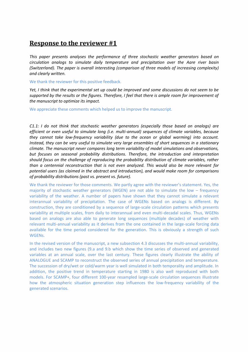
In the revised version of the manuscript, a new subsection 4.3 discusses the multi-annual variability, and includes two new figures (9.a and 9.b which show the time series of observed and generated variables at an annual scale, over the last century. These figures clearly illustrate the ability of ANALOGUE and SCAMP to reconstruct the observed series of annual precipitation and temperature. The succession of dry/wet or cold/warm year is well simulated in both temporality and amplitude. In addition, the positive trend in temperature starting in 1980 is also well reproduced with both models. For SCAMP+, four different 100-year resampled large-scale circulation sequences illustrate how the atmospheric situation generation step influences the low-frequency variability of the generated scenarios.

C1.2: Does the comparison of seasonal precipitations (Fig. 6) depend on choices of predictors to compute analogues, or even how the seasonality is taken into account?

In a preliminary work (not shown in the manuscript), we have considered many different versions of each WGEN based on different sets of predictors respectively. The set of predictors considered in our manuscript has been selected so as to maximize the skill of the WGEN for the prediction of the daily precipitation and temperature observations over the whole simulation period (Chardon et al. 2016, Raynaud et al. 2018). The skill is estimated with the Continuous Ranked Probability Skill Score (CRPSS), a probabilistic evaluation score typically used for the verification of probabilistic or ensemble weather forecasts. A comment has been added at l. 180-184.

These preliminary analyses showed that the results of the generations depend on the choice of predictors used for the analog selection. This could have been presented in our manuscript. However, results obtained with other predictor sets are not really relevant to consider. The lower skill of these other sets for the prediction of daily variables directly translates to a lower skill for the reproduction of observed seasonal probability distributions.

For the second part of the question, the seasonality is accounted for in different ways:

1. As indicated in Section 3.3.1 of the manuscript, the large-scale predictors are likely to differ from one season to the other. In our work, the first level analogy variables used to identify the candidate analog days are the same but the second level analogy variables differ according to the season. From September to May they are the vertical velocities at 600 hPa and the large scale temperature at 2 meters. In summer, the vertical velocities but also other predictors such as the Convective Available Potential Energy (CAPE) led to a rather poor prediction of precipitation due to the coarse resolution of the atmospheric reanalysis that prevent it from providing an accurate simulation of convective processes. Consequently, large scale precipitation from the reanalysis has been used instead, resulting in predictive skills similar to the ones obtained for the rest of the year.

2. The large-scale / small scale downscaling relationship is likely to differ from one season to the other. To account for this, the candidate analogs are identified within a 2 months calendar moving window centered on the target day (day of simulation). For instance, when the current simulation day is a 6th June, all days between the 6th of May and the 6th of July of each year are considered as candidate analogs. This calendar constraint for the selection of candidates was not indicated in the manuscript and this point has been added to the revised manuscript (l. 176-179).

3. A last calendar constraint is used for the first step of SCAMP+ (generation of large scale circulation sequences). This constraint is given at l. 285-287 of the present manuscript version: “To insure that two consecutive days of the generated sequences belong to the appropriate season, the five 2-day analogue sequences are identified within a +/-15-day moving window centered on the calendar day of the target simulation day (e.g. all June days if the target day is xxxx-06-15th).”

Different modifications have been made to section 3.3.1 in order to clarify these points. C1.3: I am surprised that the discussion of the results is so qualitative: the authors show boxplots or return value plots that yield rather small changes, but never compute actual scores of performance that would quantify the performance of the simulations. Continuous Rank Probability Scores (CRPS) or Tallagrand diagrams (or just quantile plots) would be more useful than a subjective appreciation of Fig. 7.

We could present the CRPSS or Tallagrand diagrams obtained for the ANALOG and the SCAMP models. Both models are indeed expected to reproduce the time variations of observed precipitation. This is not the case for SCAMP+. SCAMP+ produces its own trajectories of large-scale variables. These trajectories are by construction different from the observed one. As a result, the time series of weather variables generated with SCAMP+ are not expected to fit the observed ones.

Note in addition that the main interest of SCAMP+ is that it allows exploring a greater diversity of weather configurations and sequences. This is highlighted by the larger range obtained with SCAMP+ for different weather characteristics. A quantitative assessment of SCAMP+ via its ability to reproduce the observed sequence of some variables is thus not really relevant nor interesting. C1.4: I see no discussion of uncertainties of the results (e.g. with respect to model parameters).

It is true that a discussion on this issue should be incorporated. Among the model parameters that can have an impact on the results, we can stress the importance of:

1. the set of predictors used in the selection of analogs.

2. the number of analogs selected as potential candidates (100 for the first level of analogy and 30 for the second level).

3. the transition probability p between large scale trajectory in the first-generation step of SCAMP (p=1/7 in the manuscript).

A paragraph has been added at l. 450-455 in the section “Discussion”. C1.5: My bet for the strange performance of SCAMP+ to simulate a reasonable range of summer temperatures is that summer temperature follow a distribution that depends on the mean state (e.g. Parey, S., Dacunha-Castelle, D., & Hoang, T. H. (2010). Mean and variance evolutions of the hot and cold temperatures in Europe. Climate dynamics, 34(2-3), 345-359.). Just perturbing with a Gaussian distribution with a fixed variance lowers the variance, with respect to the true temperature variance.

Thanks for this comment. First, we would like to stress the fact that a Gaussian distribution is used only in both SCAMP and SCAMP+ models. As only SCAMP+ seems unable to generate extremely hot summers (i.e. mean summer temperature above 17°C), it cannot be attributed to this particular feature. It must also be noticed that the Gaussian distribution is applied to the 30 mean areal temperature values obtained from the analogues, for each prediction day. This setting is quite different from Parey, S., Dacunha-Castelle, D., & Hoang, T. H. (2010) who analyze directly temperature series.

Additional analyses have been made to investigate this particular issue for SCAMP+. One hypothesis is that the positive trend in temperature experienced over the 20th century would be responsible for this limitation. Indeed the new weather associations made by the random atmospheric trajectories are mixing days from the 1900s with other from the 2000s, their geopotential analogy being their only selection criteria. This could result in less chance to generate very hot summers (as observed in 2003) or very cold winters (as experienced in 1963). To verify the statement, the boxplot on winter and summer temperature have been regenerated using a modified observed series of temperature for which the trend have been removed (following the method proposed to Evin et al., 2018b, see their section 2.2.1). The results are presented on Fig. R1 below and should be compared to Fig. 7b in the manuscript. One can notice that very little improvement can be seen and that the global temperature increase is not responsible for the non-occurrence and of extremely cold winters and hot summers in SCAMP+ scenarios. Another hypothesis would consist in questioning the predictor used to generate the atmospheric trajectories in SCAMP+. In the approach presented in this study, we used the geopotential height at 1000hPa on two consecutive days. Such a choice guarantees similar positions of high/low pressure systems and comparable movements of these features for the target day and its analogues. However, no conditions on the air mass temperature have been included. In the observed archive of synoptic meteorology, two similar geopotential fields can have rather different air mass temperature. Thus, using only HGT1000 as predictor, only guarantees that the transition from one atmospheric trajectory to another is correct in terms of anticyclonic or unsettled weather. This might results in breaking series of hot/cold days. A possible improvement of

the method would be to explore more complex analogy models to generate the atmospheric trajectories in order to improve the simulation and heat and cold waves. A comment has been added at l. 470-478 to include this discussion.

Fig.10: Observed and simulated boxplots of mean seasonal temperature for models ANALOGUE, SCAMP and

SCAMP+. The temperature trend due to climate change has been removed in the daily observed time series

which is used thereafter to compute the OBS boxplot and to feed all three models. (Summer: June, July,

August. Winter: December, January, February).

Evin, Guillaume, Anne-Catherine Favre, and Benoit Hingray. 2018. “Stochastic Generators of Multi-Site Daily Temperature: Comparison of Performances in Various Applications.” Theoretical and Applied Climatology, February, 1–14. https://doi.org/10.1007/s00704-018-2404-x.

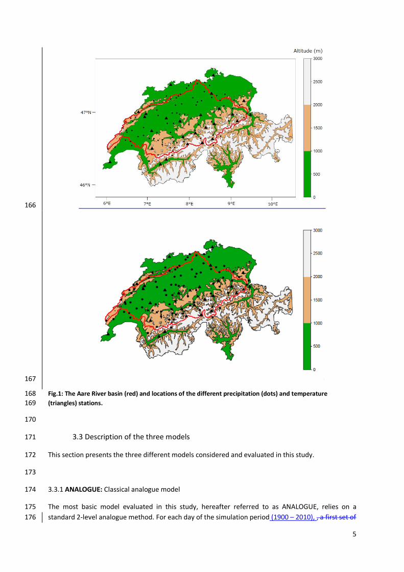
C1.6: My notions of Alpine geography are rather limited. Indications of longitude and latitude in Fig. 1 would be useful.

Longitudes and latitudes have been added in Fig. 1. C1.7: Using geopotential heights for analogs is certainly a good idea, but the authors should be aware of long term trends (due to temperature increase), which induce biases in analog computations, especially in ERA20C. The authors could consider removing such a trend.

This issue is indeed potentially critical. We use geopotential heights for the first analogy level in the analog selection. The Teweles–Wobus score (TWS) proposed by Teweles and Wobus (1954) is used there. This score has been found to lead to higher performances than a more classical Euclidian or Malahanobis distance (Kendall et al. 1983; Guilbault et Obled, 1998; Wetterhall et al., 2005). It quantifies the similarity between two geopotential fields by comparing their spatial gradients. It allows selecting dates that have the most similar spatial patterns in terms of atmospheric circulation at a given (or several) geopotential level(s). As a consequence, it does not compare the absolute values of the geopotential fields between 2 days. We are aware that the mean value of geopotential fields is expected to change with regional warming. The Teweless-Wobus has the great advantage to remove the influence of this long term trend, and should therefore avoid biases for the analog identification.

A paragraph has been added at l. 186-191 to indicate the use of this score in the description of the ANALOGUE model: “The analogy criterion used here is the Teweles–Wobus score (TWS) proposed by Teweles and Wobus (1954). This score has been found to lead to higher performances than a more

classical Euclidian or Malahanobis distance (Kendall et al. 1983; Guilbault et Obled, 1998; Wetterhall et al., 2005). It quantifies the similarity between two geopotential fields by comparing their spatial gradients. It allows selecting dates that have the most similar spatial patterns in terms of atmospheric circulation.”

In addition, a paragraph has been added to the discussion at l. 486-497 concerning potential long-term trends in the predictors: “Trends in observed predictors and predictands, as a result of global warming, could be an additional issue. For instance, the mean elevation of geopotential fields is often expected to increase with mean temperature. Such trends may be detrimental for the simulations, because the analogues identification process would be carried out in a non-homogenous data-set. In the present work for instance, trends in the second analogy level predictors (VV600, P and T) might result, to some extent, in selecting analogues preferentially within the same decade rather than distant ones. This could then reduce the reshuffling potential of the method. This issue is likely to be less critical for the first analogy level of SCAMP and for the generation of atmospheric trajectories in SCAMP+. In this case, analogues are selected according to the Teweles–Wobus score which compares the shapes of geopotential fields and not their absolute values. Quantifying the similarity between these geopotential fields, instead of differences in magnitude, removes the influence of a potential long term trend in this predictor.”

Kendall, M., Stuart, A., Ord, J.K., 1983. The Advanced Theory of Statistics. Design and Analysis, and Time-series, vol. 3. Oxford Univ Press, New York. 780 p.

Teweles J, Wobus H. 1954. Verification of prognosis charts. Bulletin of the American Meteorological Society 35: 2599–2617.

Guilbaud S, Obled C. 1998. Prévision quantitative des précipitations journalières par une technique de recherche de journées antérieures analogues: optimisation du critère d’analogie (Daily quantitative precipitation forecast by an analogue technique: optimisation of the analogy criterion). Comptes Rendus de l’Académie des Sciences – Series IIA, Earth and Planetary Science Letters 327: 181–188. doi:10.1016/S1251-8050(98)80006-2.

Wetterhall F, Halldin S, Xu CY. 2005. Statistical precipitation downscaling in central Sweden with the analogue method. Journal of Hydrology 306: 174–190. doi:10.1016/j.jhydrol.2004.09.008. C1.8: The authors compare (with two different visualizations) 1 day, 3 days, 5 days (Fig. 8) and 92 days (Fig. 7a) precipitation values. What is the cut-off duration for which the three weather generators give similar results (Fig. 7a)? If a generalized Pareto distribution was fitted to precipitation, would the ANALOGUE or SCAMP weather generators be within confidence intervals?

We thank the reviewer for this comment. In Fig.7, we assess some features of the climatology, i.e. the distribution of the precipitation amounts at the seasonal scale. We also present the seasonality and precipitation values at the monthly scale in Fig. 6. We could also present the same results at the weekly or daily scale, but it does not present so much interest since it will be very similar scaled results (i.e. the monthly mean is equal to the daily mean times the number of days in the month).

In Fig. 8, we have a look at the features of extreme values for different durations. When precipitation values are aggregated at higher temporal scales (e.g. at the monthly scale), annual maxima are not “extremes” in the sense of the extreme value theory (i.e. the maxima of samples of infinite size) and their distribution converges slowly to a Gaussian distribution and the highest intensities are tempered. In Fig. R2 below, we replicate Fig. 8 for higher aggregation durations (7 days, 15 days and 30 days). For 15-day annual maxima, differences between the ANALOGUE and SCAMP are less pronounced. For 30-day annual maxima, SCAMP+ still tends to simulate higher intensities than ANALOGUE and SCAMP models.

Concerning the last question, we show 90% - confidence intervals obtained from a GEV distribution fitted to precipitation observations in Fig. R3 below, along with the intervals obtained from the ANALOGUE and SCAMP simulations. Confidence intervals partly overlap but the confidence intervals from the GEV distribution does not recover entirely the bands obtained from the weather generators.

Fig. R2: Return level analysis of extreme precipitation values associated to model ANALOGUE, SCAMP and SCAMP+ for accumulation over 7, 15 and 30 days. The grey shadings present the inter-quantiles intervals at 50%, 90% and 99% levels (30 x 111-year scenarios for models ANALOGUE and SCAMP and 300 x 100-year scenarios for SCAMP+).

Fig. R3: Return level analysis of extreme precipitation values associated to model ANALOGUE, SCAMP and SCAMP+ for accumulation over 7, 15 and 30 days. The grey shadings present the inter-quantiles intervals at a 90%-level (30 x 111-year scenarios for models ANALOGUE and SCAMP and 300 x 100-year scenarios for SCAMP+) and the red shadings present the confidence intervals at a 90%-level obtained from the fit of a GEV distribution.

Response to the reviewer #2 This paper compares three different weather generators (WG) based on flow analogues and stochastic weather generators, including a new technique. They analyse the properties of the time series produced by these WG, with a focus on their ability to simulate extremes of precipitation and temperature. I find this paper very interesting and well written.

We thank the reviewer for this very positive feedback. I just have a few minor questions for the authors.

We appreciate these comments, the manuscript has been revised accordingly. C1: I am not sure I understand how you link the station data with the reanalyses data. If you use them to calculate daily MAP and MAT of your analogues, how do you calculate daily MAP and MAT for the 1900-1930 period for which you have ERA-20C data but no station data? Do you only use station data as your observation to which you compare the WG’s simulations?

For the period 1900-1930, it is true that only atmospheric reanalyses are available, as station data are available from 1930 to 2014. As a consequence, possible analogue candidates are only seeked during the period 1930 to 2014, for which reanalysis and station data are available. For the period 1900-1930, analogues are thus sampled among possible dates in the period 1930-2014. The statistical link between the large-scale atmospheric configuration and the small-scale weather is thus inferred from 84 years and used in a “temporal extrapolation mode” to simulate the weather of a period where we only have the large-scale information. This has been clarified in Section 3.3.1: “For each day of the simulation period (1900 – 2010), analogue days are identified from candidate days. The candidate days, extracted from the archive period, i.e. the period on which both predictors and local observations are available (1930 – 2010), are all days of the archive located within a 61-day calendar window centred on the target day.”

As a consequence, also, the results of our simulations are compared to observations that do not correspond to the same period. The simulations cover 110 years and the observations 84 years (for all figures from 4 to 8). The new figures Fig. 9a and 9b showing the time series of observed and simulated annual values should also help clarifying this point. C2: Could you specify the distance you use to calculate analogues?

Analogues are selected according to the Teweles–Wobus score (TWS) proposed by Teweles and Wobus (1954). This score has been found to lead to higher performances than a more classical Euclidian or Malahanobis distance (Kendall et al. 1983; Guilbault et Obled, 1998; Wetterhall et al., 2005). It quantifies the similarity between two geopotential fields comparing their spatial gradients. It allows selecting dates that have the most similar spatial patterns in terms of atmospheric circulation at a given (or several) geopotential level(s). As a consequence, it does not compare the absolute values of the geopotential fields between 2 days. A paragraph has been included in the revised version of the manuscript at l. 186-190. Furthermore, for the second level of analogy in models ANALOGUE and SCAMP, a sub-selection of 30 analogues within the 100 analogues identified in the first analogy level according to the Root Mean Square Error (RMSE). A comment has been added at l. 198-200.

Kendall, M., Stuart, A., Ord, J.K., 1983. The Advanced Theory of Statistics. Design and Analysis, and Time-series, vol. 3. Oxford Univ Press, New York. 780 p.

Teweles J, Wobus H. 1954. Verification of prognosis charts. Bulletin of the American Meteorological Society 35: 2599–2617.

Guilbaud S, Obled C. 1998. Prévision quantitative des précipitations journalières par une technique de recherche de journées antérieures analogues: optimisation du critère d’analogie (Daily quantitative precipitation forecast by an analogue technique: optimisation of the analogy criterion). Comptes Rendus de l’Académie des Sciences – Series IIA, Earth and Planetary Science Letters 327: 181–188. doi:10.1016/S1251-8050(98)80006-2.

Wetterhall F, Halldin S, Xu CY. 2005. Statistical precipitation downscaling in central Sweden with the analogue method. Journal of Hydrology 306: 174–190. doi:10.1016/j.jhydrol.2004.09.008. C3: Why do you use HGT1000 rather than SLP?

Raynaud et al. 2017 analysed the predictive skills of numerous atmospheric predictors and more particularly of geopotentials. They selected HGT1000 rather than SLP to compare the sensibility of the results to different geopotential levels (500, 700 or 1000hPa). However, when using the Teweles–Wobus distance SLP and HGT1000 would give very similar results as the positions of highs, of lows and the gradients are quite comparable between 1000hPa and ground level.

Raynaud, D., Hingray, B., Zin, I., Anquetin, S., Debionne, S., & Vautard, R. (2017). Atmospheric analogues for physically consistent scenarios of surface weather in Europe and Maghreb. International Journal of Climatology, 37(4), 2160-2176. C4: The first time you introduce the term "scenario", I would define what you mean by scenario right away. As you surely know this word has several different meanings in climate science so it can be a bit confusing if you do not define it clearly.

We thank the reviewer for this suggestion. In this paper, a scenario indicates a possible realization of the climate for the considered period. Indeed, it differs from climate projections which are also including prescribed projections of socioeconomic global changes. A comment has been added in the revised manuscript at l. 156-158: “a scenario is defined as a possible realization of the climate system under current climate conditions (i.e. the climate observed for the past few decades).”. C5: In the discussion, when you discuss the problem to produce temperature extremes because of climate change, you can expend this to extreme precipitations. There is an observed and projected trend on precipitation extremes related to anthropogenic climate change related to the Clausius-Clapeyron relationship.

We thank the reviewer for this comment. Concerning long-term trends, a more general discussion has been added at l. 480-485 “However, long-term fluctuations do not seem to be efficiently generated (at least for temperature). These types of variations are actually driven by very large scale or global phenomena such as the Atlantic Multi-decadal-Oscillation (AMO – Hurrell and al., 1997; Trigo et al., 2002 and Roger et al., 1997). In SCAMP+, we do not account for such driving phenomena. Introducing additional drivers such as the AMO index in the generation of atmospheric trajectories could improve the results in this respect.”

1

Assessment of meteorological extremes using a synoptic weather generator and a downscaling 1

model based on analoguesanalogs 2

Damien Raynaud1, Benoit Hingray2, Guillaume Evin3*, Anne-Catherine Favre1, Jérémy Chardon1 3

1: Univ. Grenoble Alpes, Grenoble-INP, IGE UMR 5001, Grenoble, F-38000, France 4

2: Univ. Grenoble Alpes, CNRS, IGE UMR 5001, Grenoble, F-38000, France 5

3: Univ. Grenoble Alpes, Irstea, UR ETNA, Grenoble, France. 6

*Correspondence to: Guillaume Evin (guillaume.evin@irstea.fr) 7

1. Abstract 8

Natural risk studies such as flood risk assessments require long series of weather variables. As an 9 alternative to observed series, which have a limited length, these data can be provided by weather 10 generators. Among the large variety of existing ones, resampling methods based on analogues have 11 the advantage of guaranteeing the physical consistency between local weather variables at each time 12 step. However, they cannot generate values of predictands exceeding the range of observed values. 13 Moreover, the length of the simulated series is typically limited to the length of the synoptic 14 meteorologicalmeteorology records used to characterize the large-scale atmospheric configuration 15 of the generation day. To overcome thesethose limitations, the stochastic weather generator 16 proposed in this study combines two sampling approaches based on atmospheric analogues: 1) a 17 synoptic weather generator in a first step, which recombines days ofin the 20th century to generate a 18 1,000-year sequence of new atmospheric trajectories and 2) a stochastic downscaling model in a 19 second step, applied to these atmospheric trajectories, in order to simulate long time series of daily 20 regional precipitation and temperature. The method is applied to daily time series of mean areal 21 precipitation and temperature in Switzerland. It is shown that the climatological characteristics of 22 observed precipitation and temperature are adequately reproduced. It also improves the 23 reproduction of extreme precipitation values, overcoming previous limitations of standard 24 analogueanalog-based weather generators. 25 26

2. Introduction 27

Increasing the resilience of socio-economic systems to natural hazards and identifying the required 28 adaptations is one of today’s challenges. To achieve such a goal, one must have an accurate 29 description of both past and current climate conditions. The climate system is a complex machine 30 which is known to fluctuate at very small time scales but also at large ones over multiple decades or 31 centuries (Beck et al. 2007). It is necessary to study meteorological series as long as possible in order 32 to catch all sources of variability and fully cover the large panel of possible meteorological situations. 33 Regarding weather extremes, the same need arises as estimating return levels associated to large 34 return periods cannot be successfully done without long climatic records (e.g. Moberg et al., 2006; 35 Van den Besserlaar et al., 2013). This comment also applies to all statistical analyses on any derived 36 variable, such as river discharge, for which multiple meteorological drivers come into play and for 37 which extreme events correspond to the combination of very specific and atypical hydro-38 meteorological conditions. 39

40

2

Using weather generators, long simulations of weather variables provide accurate descriptions of the 41 climate system and can be used for natural hazard assessments. Among the large panel of existing 42 weather generators, stochastic ones are used to construct, via a stochastic generation process, single 43 or multisite time series of predictands (e.g. precipitation, temperature) based on the distributional 44 properties of observed data. These characteristics, and consequently the weather generator 45 parametrisation, are usually determined on a monthly or seasonal basis to take seasonality into 46 account. They can also be estimated for different families of atmospheric circulation, often referred 47 to as weather types. A state of the art of the most common methods which have been used for the 48 downscaling of precipitation (single or multi-site) is presented in Wilks (2012) or in Maraun et al., 49 (2010). More recent publications gather detailed reviews of some sub-categories of weather 50 generators (e.g. Ailliot et al., 2015 for hierarchical models). An increasing number of studies focuses 51 on the generation of multivariate and/or multi-site series of predictands (e.g. Steinschneider and 52 Brown, 2013; Srivastav and Simonovic, 2015; Evin et al. 2018a; Evin et al. 2018b). Stochastic weather 53 generators are able to produce large ensembles of weather time series presenting a wide diversity of 54 multiscale weather events. For all these reasons, they have been used for a long time to enlighten 55 the sensitivity and possible vulnerabilities of socio-eco-systems to the climate variability (Orlowsky et 56 al. 2010) and to weather extremes. 57 58 OtherAnother family of models used for the generation of weather sequences are based onis the 59 analogue method. Since the description of the concept of analogy by Lorenz (1969), the analogue 60 method has gained popularity over time for climate or weather downscaling. This analogue model 61 strategy has been applied in many studies (Boe et al., 2007; Abatzoglou and Brown, 2012; 62 Steinschneider and Brown 2013) and has been used to address a wide range of questions from past 63 hydroclimatic variability (e.g. Kuentz et al, 2015; Caillouet et al., 2016) to future hydrometeorological 64 scenarios (e.g. Lafaysse et al., 2014; Dayon et al., 2015). The standard analogue approach 65 hypothesises that local weather parameters are steered by synoptic meteorology. A set of relevant 66 large scale atmospheric predictors is used to describe synoptic weather conditions. From the 67 atmospheric state vector, characterizing the synoptic weather of the target simulation day, 68 atmospheric analogues of the current simulation day are identified in the available climate archive. 69 Then, the analogue method makes the assumption that similar large scale atmospheric conditions 70 have the same effectseffect on local weather. The local or regional weather configuration of one of 71 the analogue days is then used as a weather scenario for the current simulation day. The key element 72 of the analogue method is that it does not require any assumption on the probability distributions of 73 predictands. This is a noteworthy advantage for predictands, such as precipitation, which have a non-74 normal distribution with a mass in zero. Most of the studies using analogues focused on precipitation 75 and temperature either for meteorological analysis (Chardon, 2014; Daoud, 2016), or as inputs for 76 hydrological simulations (Marty, 2012; Surmaini et al., 2015). Nevertheless, analogues are 77 increasingly used for other local variables such as wind, humidity (Casanueva et al., 2014) or even 78 more complex indices (e.g. for wild fire, Abatzoglou and Brown, 2012). When multiple variables are 79 to be downscaled simultaneously, another major advantage of the analogue method is that the 80 different predictands scenarios are physically consistent and the simulated weather variables are 81 bound to reproduce the correlations between the variables (e.g. Raynaud et al., 2017) and sites 82 (Chardon et al., 2014). Indeed, when analogue models use the same set of predictors (atmospheric 83 variables and analogy domains) for all predictands, all surface weather variables and sites are 84 sampled simultaneously from the historical records, thus preserving inter-site and inter-variable 85 dependency. 86 87 The two simulation approaches (stochastic weather generators and analogueanalog methods) 88 described above present some important advantages for the generation of long weather series but 89 also some sizeable drawbacks. Indeed, stochastic weather generators rely on strong assumptions 90 abouton the statistical distributions of predictands. Identifying the relevant mathematical 91 representations of the processes and achieving a robust estimation of their parameters can be 92

3

difficult, especially if the length of the meteorological records is short. Modelling the spatial-93 temporal dependency between variables/sites is often anotheran additional challenge. Conversely, 94 for the analogue-based approaches, the identification of relevant atmospheric variables providing 95 good prediction skills is not straightforward. The limited length of local weather records is also a 96 critical issue since resampling past observations restricts the range of predicted values. In particular, 97 the simulation of unobserved values of predictands is not possible. This can be problematic if one is 98 interested in estimating possible extreme values of the considered variable. Furthermore, the 99 information on synoptic atmospheric conditions required by analogueanalog methods are generally 100 coming from atmospheric reanalyses, which also have a limited temporal coverage (e.g. from the 101 beginning of the 20th century for ERA20C, Poli et al., 2013) and from the mid-19th century for 20cr 102 (Compo et al. 2011). The length of the generated time series is thus typically bounded by the length 103 of the reanalyses. 104 105 In this study we propose a weather generator (hereafter SCAMP+) building upon the SCAMP 106 approach presented by Chardon et al. (2018) and making use of reshuffled atmospheric trajectories, 107 following some of the developments by Buishand and Brandsma (2001) and Yiou et al. (2014). The 108 weather scenarios generated by SCAMP being limited by the coverage of the climate reanalyses, the 109 SCAMP+ model extends the pool of possible atmospheric trajectories. Using random transitions 110 between past atmospheric sequences, SCAMP+ generates unobserved atmospheric trajectories, on 111 which the 2-stage SCAMP approach can be applied. By exploring a wide variety of atmospheric 112 trajectories, SCAMP+ introduces some additional large-scale variability which improves the 113 exploration of possible weather sequences. In addition, as done in SCAMP (Chardon et al., 2018), the 114 SCAMP+ approach includes a simple stochastic weather generator which is estimated, for each 115 generation day, from the nearest atmospheric analoguesanalogs of this day. These two steps 116 (random atmospheric trajectories and random daily precipitation/temperature values) improve the 117 reproduction of extreme values, overcoming previous limitations of analogueanalog-based weather 118 generators, usually known to underestimate observed precipitation extremes. 119 120 These developments are carried out for the exploration of hydrological extremes (extreme floods) of 121 the Aare River basin in Switzerland (Andres et al. 2019a,b). Meteorological forcings, i.e. temperature 122 and precipitation, are thus simulated to be used as inputs of a hydrological model, for different sub-123 basins of the Aare river basin. Meteorological simulations from SCAMP+ have been used in the Swiss 124 EXAR project1 and have proven its ability to estimate the discharge values associated to very large 125 return periods on the Aare River. In section 2, we describe in details the test region, the data and 126 three simulation approaches (a classical analogue method, referred to as ANALOGUE, SCAMP and 127 SCAMP+). Section 3 presents the main results on both climatological characteristics and extreme 128 values. Section 4 sums up the main outputs of this study and proposes some further developments 129 and analysis. 130 131

132

3. Data and Method 133

3.1 Studied region 134

This study is carried out on the Aare River basin which covers almost half of Switzerland (17,700 135

km²). The topography varies greatly within the basin with, on one hand, high mountains on its 136

southern part (maximum altitude of 4270 m, Finsteraarhorn) and on the other hand, plains on the 137

1 https://www.wsl.ch/en/projects/exar.html

4

northern part (minimum altitude of 310 m). These different characteristics coupled with the basin 138

being located at the crossroads of several climatic European influences give a wide diversity of 139

possible weather situations across the year. 140

141

3.2 Atmospheric reanalysis and local weather data 142

The application of the analogue method requires a long archive providing an accurate description of 143

both past synoptic weather patterns and local atmospheric conditions. Indeed, a wide panel of 144

meteorological situations available for resampling is necessary in order to identify the best 145

analoguesanalogs for the simulation (e.g. Van Den Dool et al., 1994 ; Horton et al., 2017). In most 146

studies, synoptic situations are provided by atmospheric reanalyses. Here, we use the ERA-20C 147

atmospheric reanalysis (Poli et al., 2013) which provide information on large scale atmospheric 148

patterns on a 6 h basis from 1900 to 2010. Data are available at a 1.25° spatial resolution. More 149

specifically, the set of predictors used for the identification of atmospheric analogues is made of the 150

geopotential height at 500 and 1000 hPa, the vertical velocities at 600 hPa, large scale precipitation 151

and temperature. The justification of these choices will be given in section 3.3.1. 152

The local and surface weather parameters of interest are retrieved from 105 weather stations for 153

precipitation and 26 weather stations for temperature, which are spread out homogeneously over 154

our target region, as presented on Figure 1. These data are available at a daily time step from 1930 to 155

2014. They have been spatially aggregated in order to obtain daily time series of mean areal 156

precipitation (MAP) and temperature (MAT) for the Aare region. The three weather generators 157

considered in this study aims at producing scenarios of daily time series of MAP and MAT. In this 158

study, a scenario is defined as a possible realization of the climate system under current climate 159

conditions (i.e. the climate observed for the past few decades). It can be noticed that many 160

applications of analogue-based approaches produce simulations at specific weather stations. 161

However, as shown by Chardon et al. (2016) for France, the prediction skill is significantly improved 162

when the prediction is produced for areal averages, which motivates the generation of MAP and 163

MAT values in this study. 164

165

5

166

167

Fig.1: The Aare River basin (red) and locations of the different precipitation (dots) and temperature 168

(triangles) stations. 169

170

3.3 Description of the three models 171

This section presents the three different models considered and evaluated in this study. 172

173

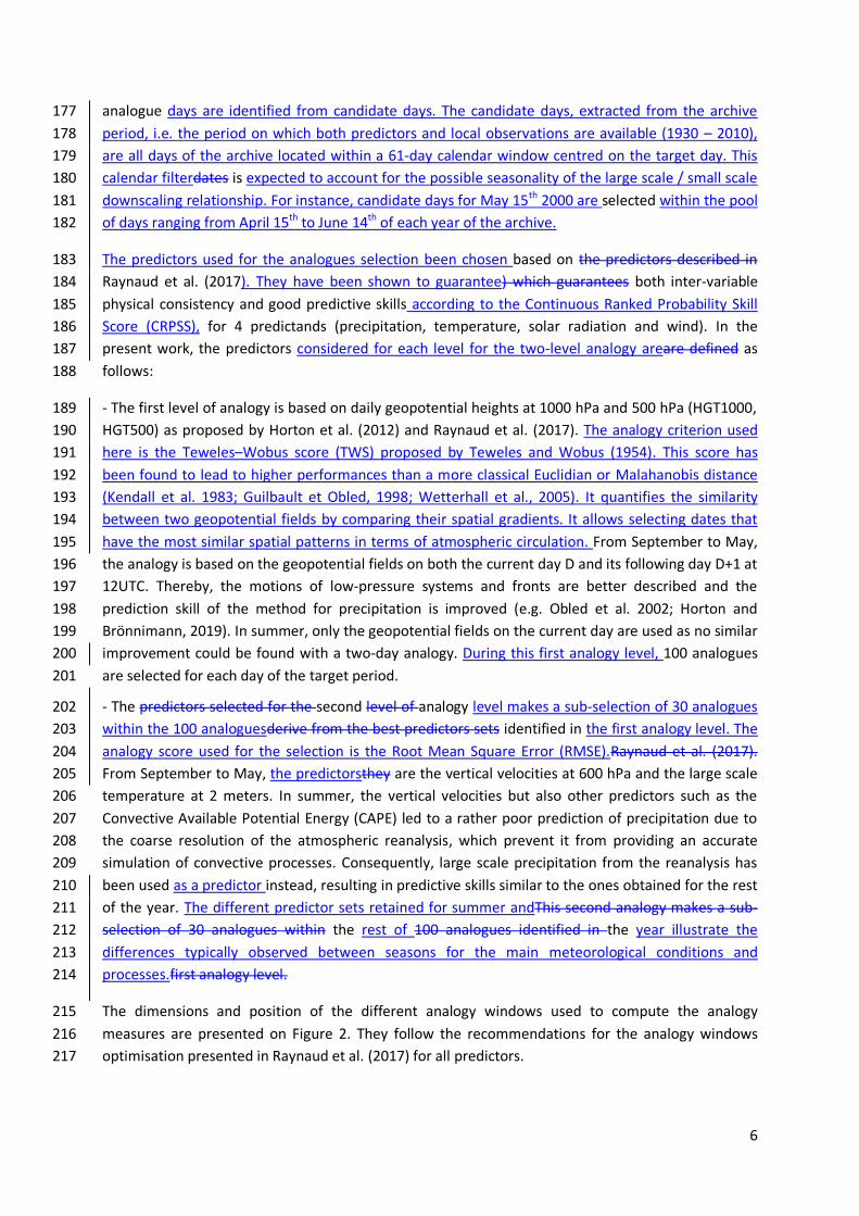
3.3.1 ANALOGUE: Classical analogue model 174

The most basic model evaluated in this study, hereafter referred to as ANALOGUE, relies on a 175

standard 2-level analogue method. For each day of the simulation period (1900 – 2010), , a first set of 176

6

analogue days are identified from candidate days. The candidate days, extracted from the archive 177

period, i.e. the period on which both predictors and local observations are available (1930 – 2010), 178

are all days of the archive located within a 61-day calendar window centred on the target day. This 179

calendar filterdates is expected to account for the possible seasonality of the large scale / small scale 180

downscaling relationship. For instance, candidate days for May 15th 2000 are selected within the pool 181

of days ranging from April 15th to June 14th of each year of the archive. 182

The predictors used for the analogues selection been chosen based on the predictors described in 183

Raynaud et al. (2017). They have been shown to guarantee) which guarantees both inter-variable 184

physical consistency and good predictive skills according to the Continuous Ranked Probability Skill 185

Score (CRPSS), for 4 predictands (precipitation, temperature, solar radiation and wind). In the 186

present work, the predictors considered for each level for the two-level analogy areare defined as 187

follows: 188

- The first level of analogy is based on daily geopotential heights at 1000 hPa and 500 hPa (HGT1000, 189

HGT500) as proposed by Horton et al. (2012) and Raynaud et al. (2017). The analogy criterion used 190

here is the Teweles–Wobus score (TWS) proposed by Teweles and Wobus (1954). This score has 191

been found to lead to higher performances than a more classical Euclidian or Malahanobis distance 192

(Kendall et al. 1983; Guilbault et Obled, 1998; Wetterhall et al., 2005). It quantifies the similarity 193

between two geopotential fields by comparing their spatial gradients. It allows selecting dates that 194

have the most similar spatial patterns in terms of atmospheric circulation. From September to May, 195

the analogy is based on the geopotential fields on both the current day D and its following day D+1 at 196

12UTC. Thereby, the motions of low-pressure systems and fronts are better described and the 197

prediction skill of the method for precipitation is improved (e.g. Obled et al. 2002; Horton and 198

Brönnimann, 2019). In summer, only the geopotential fields on the current day are used as no similar 199

improvement could be found with a two-day analogy. During this first analogy level, 100 analogues 200

are selected for each day of the target period. 201

- The predictors selected for the second level of analogy level makes a sub-selection of 30 analogues 202

within the 100 analoguesderive from the best predictors sets identified in the first analogy level. The 203

analogy score used for the selection is the Root Mean Square Error (RMSE).Raynaud et al. (2017). 204

From September to May, the predictorsthey are the vertical velocities at 600 hPa and the large scale 205

temperature at 2 meters. In summer, the vertical velocities but also other predictors such as the 206

Convective Available Potential Energy (CAPE) led to a rather poor prediction of precipitation due to 207

the coarse resolution of the atmospheric reanalysis, which prevent it from providing an accurate 208

simulation of convective processes. Consequently, large scale precipitation from the reanalysis has 209

been used as a predictor instead, resulting in predictive skills similar to the ones obtained for the rest 210

of the year. The different predictor sets retained for summer andThis second analogy makes a sub-211

selection of 30 analogues within the rest of 100 analogues identified in the year illustrate the 212

differences typically observed between seasons for the main meteorological conditions and 213

processes.first analogy level. 214

The dimensions and position of the different analogy windows used to compute the analogy 215

measures are presented on Figure 2. They follow the recommendations for the analogy windows 216

optimisation presented in Raynaud et al. (2017) for all predictors. 217

7

With this 2-step analogy, 30 scenarios of daily MAP and daily MAT are obtainedgenerated for each 218

day of the simulation period (1900-2010). Combined with the Schaake Shuffle method described in 219

section 3.3.4, the application of the ANALOGUE model leads to 30 scenarios of 110-year time series 220

of daily MAP and MAT. 221

222

Fig.2: Positions and dimensions of the analogy windows in the analogue model at both analogy levels. Z500, 223

geopotential at 500 hPa ; Z1000, geopotential at 1000 hPa ; VV600, vertical velocities at 600 hPa ; P, 224

precipitation ; T, temperature. 225

226

3.3.2 SCAMP: Combined analog / generation of MAP and MAT values 227

The SCAMP model enhances the previous approach ANALOGUE approach which is not able to 228

generate daily values exceeding the range of observed precipitation and temperature. SCAMP 229

combines the analogue method with a day-to-day adaptive and tailored downscaling method using 230

daily distributions adjustment (Chardon et al. 2018). 231

For each prediction day, the following discrete-continuous probability distribution proposed by Stern 232

and Coe (1984) is fitted to the 30 MAP values obtained from the atmospheric analogues of this day: 233

𝑭𝒀(𝒚) = (𝟏 − 𝝅) + 𝝅 ∙ 𝑭𝑮𝑨(𝒚|𝒚 > 𝟎, 𝜶, 𝜷), (1) 234

where π is the precipitation occurrence probability, 𝐹𝐺𝐴 is the gamma distribution parameterized 235

with a shape parameter 𝛼 > 0 and a rate parameter 𝛽 > 0. The π parameter is directly estimated by 236

the proportion of dry days, and the parameters 𝛼, 𝛽 of the gamma distribution are estimated by 237

8

applying the maximum likelihood method to the positive precipitation intensities among the 30 MAP 238

values. 30 MAP values are then sampled from the distribution model (1) in order to obtain 239

unobserved values of precipitation, possibly beyond past observations. When there are less than 5 240

positive MAP intensities in the analogues, we simply retrieve the MAP analog values. This distribution 241

model corresponds to a simplified version of the combined analogueanalog/regression model 242

described in Chardon et al. 2018 and we refer the reader to this paper for further information. 243

Similarly, for each prediction day, a Gaussian distribution 𝐹𝑁(𝜇, 𝜎) is fitted to the 30 MAT values 244

obtained from the analogues. A sample of 30 new MAT values is then generated from this fitted 245

Gaussian distribution. 246

As for the ANALOGUE approach, the Schaake Shuffle reordering method is applied to the daily 247

scenarios obtained from SCAMP. 30 scenarios of 110-year time series of daily MAP and MAT are 248

produced. 249

250

3.3.3 SCAMP+ 251

As mentioned previously, the first limitation of the analogue method is related to the length of the 252

synoptic weather information that is used to generate local predictands time series. In the present 253

case, the length of time series that can be produced with the models ANALOGUE and SCAMP is 254

limited to 110-year long weather scenarios. 255

256

In SCAMP+, we extend the archive of synoptic weather information by rearranging the synoptic 257

weather sequences, thus creating new atmospheric trajectories, used in turn as inputs to SCAMP. 258

This generation of new trajectories makes use of atmospheric analogues, following those of the 259

principles proposed in the weather generators described by Buishand and Brandsma (2001) and Yiou 260

et al. (2014). For any given day, the atmospheric synoptic weather is considered to have the 261

possibility to change its trajectory. The main hypothesis of this generation module is that if two days 262

J and K are close atmospheric analogues with atmospheric patterns heading in the same direction, 263

then their “future” are exchangeable and one could jump from one atmospheric trajectory to the 264

other. In other words, day J+1 is a possible future of day K and conversely day K+1 is a possible future 265

of day J. The probability p to jump from one trajectory to any other is considered as a parameter to 266

estimate. 267

268

The principle of a random atmospheric trajectory generation is sketched on Figure 3. In the present 269

work, the only predictor involved to compare the synoptic atmospheric configuration between 2 270

different days is the geopotential height field at 1000 hPa, for both the present day and its followers. 271

The spatial analogy domain is the one used in Philipp et al. (2010) for the identification of Swiss 272

weather types. The first line of Figure 3 presents an observed atmospheric trajectory in HGT1000 273

from February 8th to February 12th 1934. On the February 9th, we look for analogues of the current 274

day and its following day D+1. This is done to ensure that the two initial states are similar (high 275

pressure system located over France on February 9th 1934 and on its analogue, January 28th 1921) 276

and that the main features move in similar directions (high pressure system heading South-East on 277

both February 10th 1934 and January 29th 1921). 278

279

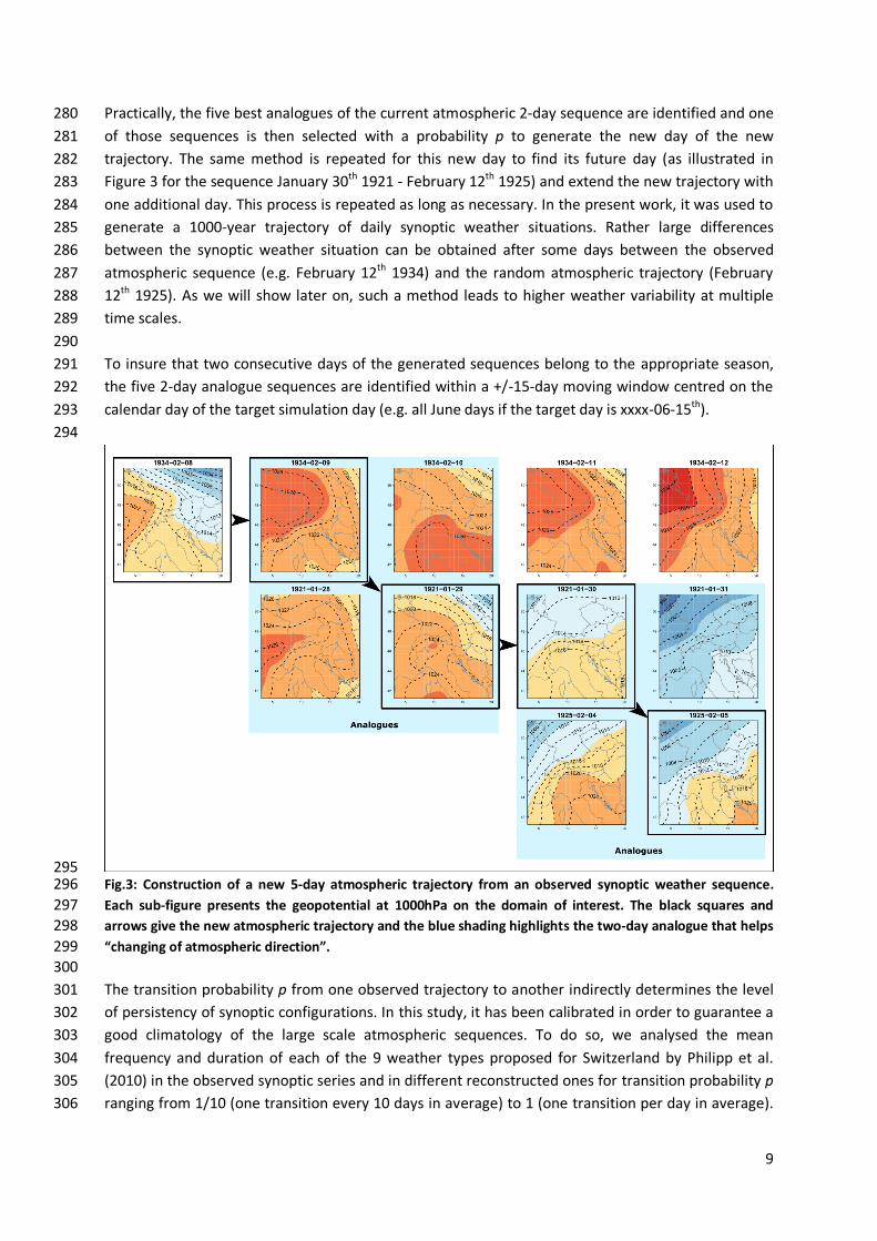
9

Practically, the five best analogues of the current atmospheric 2-day sequence are identified and one 280

of those sequences is then selected with a probability p to generate the new day of the new 281

trajectory. The same method is repeated for this new day to find its future day (as illustrated in 282

Figure 3 for the sequence January 30th 1921 - February 12th 1925) and extend the new trajectory with 283

one additional day. This process is repeated as long as necessary. In the present work, it was used to 284

generate a 1000-year trajectory of daily synoptic weather situations. Rather large differences 285

between the synoptic weather situation can be obtained after some days between the observed 286

atmospheric sequence (e.g. February 12th 1934) and the random atmospheric trajectory (February 287

12th 1925). As we will show later on, such a method leads to higher weather variability at multiple 288

time scales. 289

290

To insure that two consecutive days of the generated sequences belong to the appropriate season, 291

the five 2-day analogue sequences are identified within a +/-15-day moving window centred on the 292

calendar day of the target simulation day (e.g. all June days if the target day is xxxx-06-15th). 293

294

295 Fig.3: Construction of a new 5-day atmospheric trajectory from an observed synoptic weather sequence. 296

Each sub-figure presents the geopotential at 1000hPa on the domain of interest. The black squares and 297

arrows give the new atmospheric trajectory and the blue shading highlights the two-day analogue that helps 298

“changing of atmospheric direction”. 299

300

The transition probability p from one observed trajectory to another indirectly determines the level 301

of persistency of synoptic configurations. In this study, it has been calibrated in order to guarantee a 302

good climatology of the large scale atmospheric sequences. To do so, we analysed the mean 303

frequency and duration of each of the 9 weather types proposed for Switzerland by Philipp et al. 304

(2010) in the observed synoptic series and in different reconstructed ones for transition probability p 305

ranging from 1/10 (one transition every 10 days in average) to 1 (one transition per day in average). 306

10

The results presented on Figure 4 shows that a transition probability of 1/7 is necessary to generate 307

atmospheric trajectories that present a relevant persistency within each weather type. 308

309

Fig.4: Mean persistency of each of the 9 weather types (indicated by the different circles in each panel), as 310

defined by Philipp et al. (2010), in the observed time series and in the simulated ones for transition 311

probabilities ranging from 1 to 1/10 for the generation of atmospheric trajectories. 312

313

The long time series of synoptic weather generated with the above approach is further used as 314

inputs to the SCAMP generator described in the previous section. The SCAMP+ approach leads to 30 315

scenarios of daily MAP and MAT, each of these scenarios being based on the 1000-year random 316

atmospheric trajectories sequence. The output of this approach, combined with the Schaake Shuffle 317

method described in the next section, is thus composed of 30 scenarios of 1000-year time series of 318

daily MAP and MAT. 319

320

3.3.4 Temporal consistency: Application of the Schaake Shuffle 321

For each model (ANALOGUE, SCAMP and SCAMP+) and each day of the simulation period,+), 30 322

scenarios of daily MAP and MAT are produced. To improve the temporal/physical consistency 323

between two consecutive days or between the temperature and precipitation scenarios (partially 324

induced by the synoptic weather series), we use the Schaake Shuffle method initially proposed by 325

Clark et al. (2004). This method makes use of both the inter-variable physical and the intra-variable 326

temporal consistency in observations to combine, at best, the outputs of any weather generator and 327

reconstruct consistent predictands time series. It is particularly useful if one is interested in 328

11

generating relevant precipitation accumulation scenarios over several days. A full description of the 329

Schaake Shuffle method can be found in Clark et al. (2004) and some applications can be found in 330

Bellier et al. (2017) or in Schefzik (2017). Here, the Schaake Shuffle consists in modifying the 331

sequences of MAP and MAT values, preserving the association of the ranks of MAP and MAT and 332

rearranging sequences between days D and D+1. Shuffled MAP and MAT sequences between 333

consecutive days then have similar associations than what has been observed. In this study, we give 334

priority to the temporal consistency of precipitation first. Temperature scenarios are recombined in a 335

second step. 336

The different components of the models ANALOGUE, SCAMP and SCAMP+ are summarized in Figure 337

5. 338

339

340

Fig.5: Illustration of the different steps applied (grey boxes) with models ANALOGUE, SCAMP and SCAMP+. 341

Outputs obtained after each step are indicated in red. 342

343

4. Results 344

This section presents different statistical properties of the scenarios obtained with the 3 models and 345

discusses the performances of each model by comparison with observed statistical properties. For 346

the sake of consistency between the outputs, we compare the 30 scenarios of 111 years obtained 347

from ANALOGUE and SCAMP to 300 scenarios of 100 years from SCAMP+ (i.e. each scenario of 1,000 348

years is divided into 10 scenarios of 100 years). 349

4.1 Climatology 350

12

For both temperature and precipitation, the 3 models lead to an accurate simulation of their 351

seasonal fluctuations (Figure 6). However, one can notice the slight overestimation of winter 352

temperature and an underestimation of July and August precipitation. SCAMP also tends to have a 353

smaller inter-annual variability compared to ANALOGUE and SCAMP+. 354

355

Fig.6: Observed and simulated seasonal cycles of temperature and precipitation for ANALOGUE, SCAMP and 356

SCAMP+. The grey shadings present the inter-quantiles intervals at 50%, 90% and 99% levels.. Simulated 357

seasonal cycles are obtained using 30 scenarios of 111 years from ANALOGUE and SCAMP and 300 scenarios 358

of 100 years from SCAMP+. 359

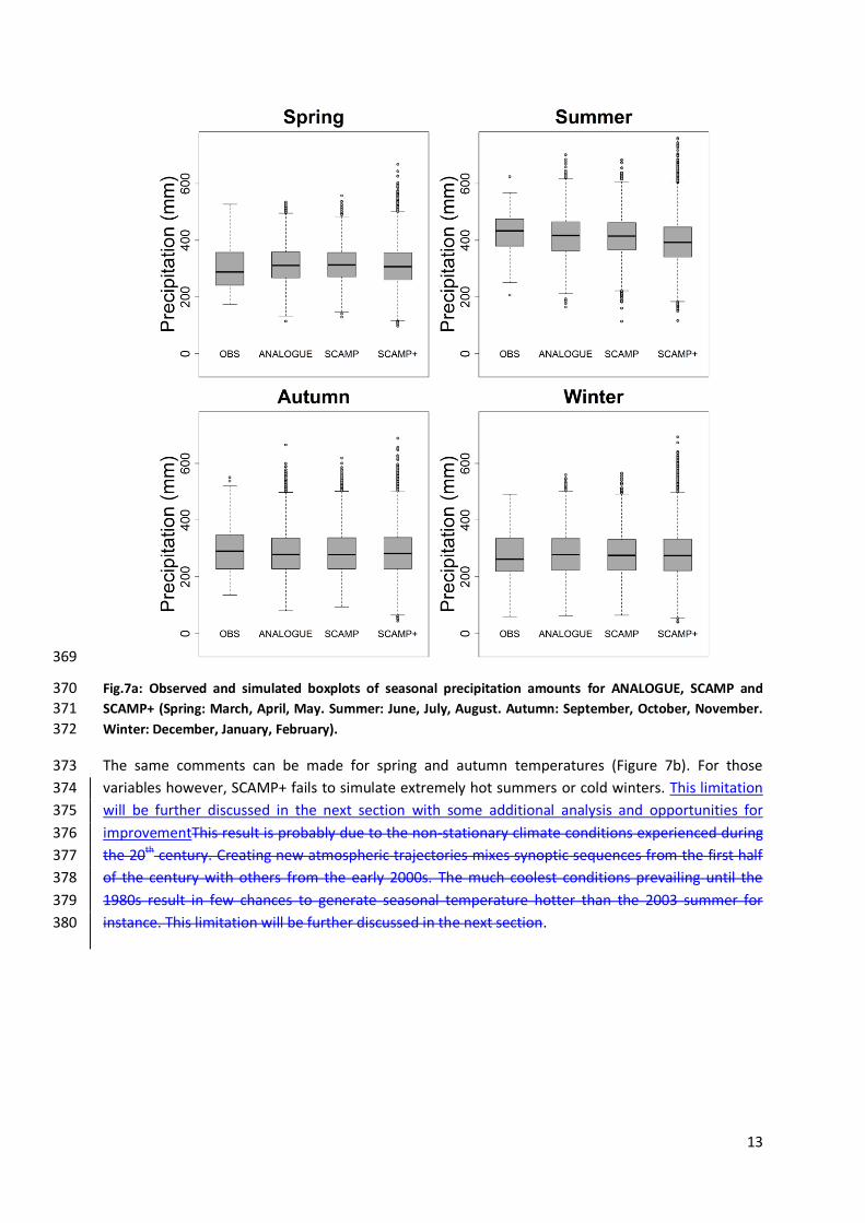
The distributions of seasonal precipitation amounts and seasonal temperature averages are 360

presented in Figure 7. Whatever the season, the three models are able to generate drier and wetter 361

seasons than the observed ones (Figure 7a). The very similar results obtained for ANALOGUE and 362

SCAMP suggest that the daily distribution adjustments used in SCAMP do not introduce more 363

variability at the seasonal scale. SCAMP+ is able to generate seasonal values that significantly exceed 364

the maximum values simulated by ANALOGUE and SCAMP (by 100 mm to 200 mm). This strongly 365

suggests that a large part of the seasonal variability comes from the variability of the synoptic 366

weather trajectories, the unobserved weather trajectories produced by SCAMP+ leading to a wider 367

exploration of extreme seasonal values. 368

13

369

Fig.7a: Observed and simulated boxplots of seasonal precipitation amounts for ANALOGUE, SCAMP and 370

SCAMP+ (Spring: March, April, May. Summer: June, July, August. Autumn: September, October, November. 371

Winter: December, January, February). 372

The same comments can be made for spring and autumn temperatures (Figure 7b). For those 373

variables however, SCAMP+ fails to simulate extremely hot summers or cold winters. This limitation 374

will be further discussed in the next section with some additional analysis and opportunities for 375

improvementThis result is probably due to the non-stationary climate conditions experienced during 376

the 20th century. Creating new atmospheric trajectories mixes synoptic sequences from the first half 377

of the century with others from the early 2000s. The much coolest conditions prevailing until the 378

1980s result in few chances to generate seasonal temperature hotter than the 2003 summer for 379

instance. This limitation will be further discussed in the next section. 380

14

381

Fig.7b: Observed and simulated boxplots of mean seasonal temperature for models ANALOGUE, SCAMP and 382

SCAMP+ (Spring: March, April, May. Summer: June, July, August. Autumn: September, October, November. 383

Winter: December, January, February). 384

385

4.2 Daily Precipitations Extremes 386

387

As mentioned in section 1, simple analogue methods cannot simulate unobserved precipitation 388

extremes at the temporal resolution of the simulation (here daily). Moreover, for higher aggregation 389

durations, they also tend to underestimate observed precipitation extremes. Figure 8 presents the 390

precipitation values obtained with the three models for different return periods (from 2 year to 200 391

years) and different aggregation durations (from 1 to 5 days). 392

393

Considering 1-day extreme events, ANALOGUE is obviously not able to generate precipitation 394

accumulations that exceed the maximum observed one. Combining the analogue method with daily 395

distribution adjustments (SCAMP) overcomes this issue with maximum values reaching 115 mm. 396

SCAMP+ leads to similar results. 397

398

15

The large underestimation of daily extremes obtained with ANALOGUE leads to an important 399

underestimation of 3-day and 5-day extremes. Despite a better simulation of daily values, SCAMP 400

does not improve significantly the reproduction of 3-day and 5-day extremes. SCAMP+ outperforms 401

both models for all durations, and generates precipitation extremes in agreement with observed 402

extremes. Whatever the return period, the variability between the different 100-year scenarios is 403

larger with SCAMP than with ANALOGUE and much larger with SCAMP+. This again suggests that 3 to 404

5-day extreme events can arise from atypical synoptic conditions, possibly not available in a 110-year 405

long weather archive. Thanks to the random atmospheric trajectories, SCAMP+ is able to generate 406

such conditions. 407

408

409

16

410

Fig.8: Return level analysis of extreme precipitation values associated to model ANALOGUE, SCAMP and 411

SCAMP+ for accumulation over 1, 3 and 5 days. The grey shadings present the inter-quantiles intervals at 412

50%, 90% and 99% levels (30 x 111-year scenarios for models ANALOGUE and SCAMP and 300 x 100-year 413

scenarios for SCAMP+). 414

4.3 Multi-annual variability 415

Figure 9.a and 9.b present examples of simulated time series of annual MAP and MAT obtained with 416

ANALOGUE and SCAMP models. Concerning SCAMP+, four (among the 10 possible scenarios) 417

illustrative time series associated to different 100-year atmospheric trajectories are shown. For all 418

models, we present the dispersion between the 30 annual values obtained from the 30 time series 419

associated to the different atmospheric trajectories. This dispersion is very small for temperature and 420

rather large in comparison for precipitation, illustrating the important uncertainty in the Large‐Scale 421

to Small‐Scale Relationship for this variable in this region. 422

For ANALOGUE and SCAMP, the simulated year-to-year variations of annual precipitation and 423

temperature are in agreement with the observed ones. The successions of dry/wet or cold/warm 424

years are well simulated in both temporality and amplitude and the positive trend in temperature 425

starting in 1980 is also adequately reproduced. Similar results are obtained for seasonal precipitation 426

17

and temperature (not shown). These results illustrate the determinant influence of the large-scale 427

conditions on local weather in this region and the relevance of a generation process based on 428

atmospheric analogues. 429

In contrast, the chronological year-to-year variations produced by the different runs of SCAMP+ 430

present different features. The annual precipitation and temperature time series obtained from 431

different runs of SCAMP+ resulting from different large-scale atmospheric trajectories, they cannot 432

be directly compared to the observed time series. This highlights the ability and interest of SCAMP+ 433

to explore non-observed sequences of precipitation and temperature at annual and multi-annual 434

scales. Finally, it must be noticed that SCAMP+ simulations are not expected to reproduce the 435

warming observed after 1980. Indeed, the different runs presented in Figure 9b are associated to 436

different 100-year subsets of the 1000-year atmospheric trajectories simulation and do not include 437

any trend (see discussion in Section 5). 438

18

439

Fig.9a: Time series of annual MAP for the ANALOGUE model (1900-2010), SCAMP (1900-2010) and 4 different 440

100-year atmospheric trajectories of SCAMP+. The observed annual MAP (1930-2014) is presented with the 441

black solid line in the plots associated to ANALOGUE and SCAMP models. The grey shadings present the 442

inter-quantiles intervals at 50%, 90% and 99% levels (30 x 111-year scenarios for models ANALOGUE and 443

SCAMP and 30 x 100-year scenarios for SCAMP+). 444

19

445

Fig.9b: Time series of annual MAT for the ANALOGUE model (1900-2010), SCAMP (1900-2010) and 4 different 446

100-year atmospheric trajectories of SCAMP+. The observed annual MAT (1930-2014) is presented with the 447

black solid line in the plots associated to ANALOGUE and SCAMP models. The grey shadings present the 448

inter-quantiles intervals at 50%, 90% and 99% levels (30 x 111-year scenarios for models ANALOGUE and 449

SCAMP and 30 x 100-year scenarios for SCAMP+). 450

20

451

452

5. Discussion and conclusions 453

The different extensions of the classical analogue method introduced in this study aims at generating 454

long regional weather time series without suffering from the main limitations of analogue models. 455

Indeed, due to the limited extent of the observed time series and the impossibility to simulate 456

unobserved daily scenarios, analogue models usually underestimate observed precipitation 457

extremes. These limitations are relaxed by SCAMP+, the weather generator proposed in this study. 458

SCAMP+ generates unobserved and plausible atmospheric trajectories, and, in addition, provides 459

unobserved samples of daily temperature and precipitation using daily distribution adjustments. 460

Such a generation process explores a larger weather variability at multiple time scales, which leads to 461

a better reproduction of precipitation extremes. 462

SCAMP+ is built upon a number of past studies carried out in the target region with Analogue-based 463

downscaling approaches. Different sensitivity analyses could be performed in order to ass the impact 464

of the different modelling choices, e.g. the set of predictors used for the analogues selection, the 465

number of analogues selected for the different analogy levels or the parameters related to the 466

generation of atmospheric trajectories (e.g. probability of transition between large scale 467

trajectories). 468

469

SCAMP+ is obviously not free of limitations. A first issue is relative to the quality of observations 470

used in the model, especially at the synoptic scale. ERA20C reanalyses used here are produced using 471

sea level pressure and wind measurements only. This guarantees a certain quality of the geopotential 472

at 1000 hPa. The quality of 500 hPa data and of the other predictors is conversely questionable 473

(namely large- scale temperature, precipitation and vertical velocities), as they do not beneficiate 474

from the assimilation of observed data. This may impact the quality of the downscaling method. For 475

instance, this could explain why the mean seasonal cycle of monthly precipitation is not well 476

reproduced in our results (see for instance the underestimation of the mean precipitation in August). 477

Using higher quality data is expected to partly address such limitations. Indeed, using ERA-Interim 478

reanalyses (Dee et al, 2011) instead of ERA20C removes the biases and mis-reproductions mentioned 479

above (not shown), a much larger panel of weather observations being assimilated in ERA-Interim. 480

However, ERA-Interim covers a much smaller time period than ERA20C (roughly 50 years). Using ERA-481

Interim for our simulations would make the panel of observed synoptic situations much less 482

representative of possible ones, and would impact the ability of our model to generate long-term 483

climate variability. Similarly, the regional predictands time series are based on 105 weather stations 484

for precipitation and 26 weather stations for temperature. The representativeness of this 485

information is also questionable, especially if one is interested in looking at precipitation and 486

temperature extreme events. However, this large number of stations leads to the best possible 487

estimations of these regional variables that can be achieved currently. 488

As highlighted previously, a noticeable limitation of SCAMP+ is its difficulty to generate very hot 489

summers or cold winters. The predictors used for the selection of the analogues may actually prevent 490

the simulation of very cold/hot seasons. Choosing the geopotential height at 1000hPa on two 491

21

consecutive days guarantees similar positions of high/low pressure systems and comparable 492

movements of these features for the target day and its analogues. This guarantees that the transition 493

from one atmospheric trajectory to another is correct in terms of anticyclonic or unsettled weather 494

but this cannot guarantee that the transition is correct in terms of air masses temperatures. This 495

might prevent the generation of long hot/cold sequences. A possible improvement of the method 496

would be to include some temperature predictor in the selection of analogue days. Similarly, 497

SCAMP+ is able to generate relevant inter-annual fluctuations of unobserved climate time series. 498

However, long-term fluctuations do not seem to be efficiently generated (at least for temperature). 499

These types of variations are actually driven by very large scale or global phenomena such as the 500

Atlantic Multi-decadal-Oscillation (AMO – Hurrell and al., 1997; Trigo et al., 2002 and Roger et al., 501

1997). In SCAMP+, we do not account for such driving phenomena. Introducing additional drivers 502

such as the AMO index in the generation of atmospheric trajectories could improve the results in this 503

respect. 504

Trends in observed predictors and predictands, as a result of global warming, could be an additional 505

issue. . For instance, the mean elevation of geopotential fields is often expected to increase with 506

mean temperature. Such trends may be detrimental for the simulations, because the analogues 507

identification process would be carried out in a non-homogenous data-set. In the present work for 508

instance, trends in the second analogy level predictors (VV600, P and T) might result, to some extent, 509

in selecting analogues preferentially within the same decade rather than distant ones. This could 510

then reduce the reshuffling potential of the method. This issue is likely to be less critical for the first 511

analogy level of SCAMP and for the generation of atmospheric trajectories in SCAMP+. In this case, 512

analogues are selected according to the Teweles–Wobus score which compares the shapes of 513

geopotential fields and not their absolute values. Quantifying the similarity between these 514

geopotential fields, instead of differences in magnitude, removes the influence of a potential long 515

term trend in this predictor. 516

Some other questions remain open, such as the difficulties encountered by SCAMP+ concerning the 517

generation of very hot summers or very cold winters. It is very likely related to the temperature 518

increase experienced over the 20th century, which appears clearly when looking at the hottest 519

summers and the coldest winters. The new weather associations made by the random atmospheric 520

trajectories are mixing days from the 1900s with other from the 2000s, their geopotential analogy 521

being their only selection criteria. This could result in less chance to generate very hot summers (as 522

observed in 2003) or very cold winters (as experienced in 1963). A possible improvement of the 523

method could be to detrend the temperature data and perform the analysis presented in this study 524

on "stationarized" temperature data (similarly to Evin et al., 2018b, see their section 2.2.1). 525

526

All in all, SCAMP+ weather generator paves the way for more developments and applications. As part 527

of the EXAR project (see acknowledgments), the model was coupled with a spatial and temporal 528

disaggregation model and fed a hydrological model in order to generate long series of discharge data 529

(Andres et al., 2019a,b). Additional evaluations on the inter-variable co-variability showed that the 530

physical consistency between temperature and precipitation is well reproduced in our simulations 531

and that the model thus efficiently simulates the precipitation phase and the statistical 532

characteristics of liquid/solid precipitation. SCAMP+ has a low computational cost and is able to 533

generate multiple weather sequences which are consistent with possible trajectories of large- scale 534

22

atmospheric conditions, which motivates future applications to other regions and other local 535

weather variables. 536

537

Data availability. 538

Precipitation and temperature data have been downloaded from Idaweb 539

(https://gate.meteoswiss.ch/idaweb/), a data portal which provides users in the field of teaching and 540

research with direct access to archive data of MeteoSwiss ground-level monitoring networks. 541

However, the acquired data may not be used for commercial purposes (e.g., by passing on the data 542

to third parties, by publishing them on the internet). As a consequence, we cannot offer direct access 543

to the data used in this study. Atmospheric predictors are taken from the European Centre for 544

Medium-Range Weather Forecasts (ECMWF) ERA20C atmospheric reanalysis (Poli et al., 2013), 545

available at the following address: https://www.ecmwf.int/en/forecasts/datasets/reanalysis-546

datasets/era-20c. 547

548

Author contributions. 549

J. Chardon and D. Raynaud developed the different models considered here. D. Raynaud carried out 550

the simulations, produced the analyses and the figures presented in this study. All authors 551

contributed to the analysis framework and to the redaction. 552

553

Competing interests. 554

The authors declare that they have no conflict of interest. 555

556

Financial support. We gratefully acknowledge financial support from the Swiss Federal Office for 557

Environment (FOEN), the Swiss Federal Nuclear Safety Inspectorate (ENSI), the Federal Office for Civil 558

Protection (FOCP), and the Federal Office of Meteorology and Climatology, MeteoSwiss, through the 559

project “Hazard information for extreme flood events on Aare River” (EXAR): 560 https://www.wsl.ch/en/projects/exar.html. 561 562

Bibliography 563

Abatzoglou, J. T., & Brown, T. J.: A comparison of statistical downscaling methods suited for wildfire 564 applications. International Journal of Climatology, 32(5), 772-780, doi:10.1002/joc.2312 , 2012. 565

Ailliot, P., Allard, D., Monbet, V., & Naveau, P.: Stochastic weather generators: an overview of weather 566 type models. Journal de la Société Française de Statistique, 156(1), 101-113, 2015. 567

Andres, N., A. Badoux, and C. Hegg. : EXAR – Grundlagen Extremhochwasser Aare-Rhein. 568 Hauptbericht Phase B. Eidg. Forschungsanstalt Für Wald, Schnee Und Landschaft WSL, 2019a. 569

Andres, N., Badoux, A., Steeb, N., Portmann, A., Hegg, C, Dang, V., Whealton, C, Sutter, A., Baer, P., 570 Schwab, S., Graf, K., Irniger, A., Pfäffli, M., Hunziker, R., Müller, M., Karrer, T., Billeter, P., Sikorska, 571 A., Staudinger, M., Viviroli, D., Seibert, J., Kauzlaric, M., Keller, L., Weingartner, R., Chardon, J., 572 Raynaud, D., Evin, G., Nicolet, G., Favre, A.C., Hingray, B., Lugrin, T., Asadi, P., Engelke, S., 573 Davison, A., Rajczak, J., Schär, C., Fischer, E.,: EXAR – Grundlagen Extremhochwasser Aare-Rhein. 574 Arbeitsbericht Phase B. Detailbericht A. Hydrometeorologische Grundlagen, WSL, Zurich, 2019b. 575

Beck, C. H., Jacobeit, J., & Jones, P. D.: Frequency and within‐type variations of large‐scale 576 circulation types and their effects on low‐frequency climate variability in central Europe since 577 1780. International Journal of Climatology, 27(4), 473-491, doi:10.1002/joc.1410, 2007. 578

23

Bellier, J., Bontron, G. and Isabella Zin.: Using Meteorological Analogues for Reordering 579 Postprocessed Precipitation Ensembles in Hydrological Forecasting. Water Resources Research, 53 580 (12): 10085–107, doi:10.1002/2017WR021245, 2017. 581

Boé, J., Terray, L., Habets, F., & Martin, E.: Statistical and dynamical downscaling of the Seine basin 582 climate for hydro‐meteorological studies. International Journal of Climatology: A Journal of the Royal 583 Meteorological Society, 27(12), 1643-1655, doi:10.1002/joc.1602, 2007. 584

Buishand, T. A., & Brandsma, T.: Multisite simulation of daily precipitation and temperature in the 585 Rhine basin by nearest‐neighbor resampling. Water Resources Research, 37(11), 2761-2776, 586 doi:10.1029/2001WR000291, 2001. 587

Caillouet, L., Vidal, J. P., Sauquet, E., & Graff, B.: Probabilistic precipitation and temperature 588 downscaling of the Twentieth Century Reanalysis over France. Climate of the Past, 12(3), 635-662, 589 doi:10.5194/cp-12-635-2016, 2016. 590

Casanueva, A., Frías, M. D., Herrera, S., San-Martín, D., Zaninovic, K., & Gutiérrez, J. M.: Statistical 591 downscaling of climate impact indices: testing the direct approach. Climatic change, 127(3-4), 547-592 560, doi:10.1007/s10584-014-1270-5 , 2014. 593

Chardon, J., Favre, A.C., Hingray, B.: Effects of spatial aggregation on the accuracy of statistically 594 downscaled precipitation estimates. J.HydroMeteorology 17: 156-1578. doi:10.1175/JHM-D-15-595 0031.1, 2016. 596

Chardon, J., Hingray, B., and Favre, A.-C.: An adaptive two-stage analog/regression model for 597 probabilistic prediction of small-scale precipitation in France, Hydrol. Earth Syst. Sci., 22, 265–286, 598 doi:10.5194/hess-22-265-2018, 2018. 599

Chardon, J., Hingray, B., Favre, A. C., Autin, P., Gailhard, J., Zin, I., & Obled, C.: Spatial similarity and 600 transferability of analog dates for precipitation downscaling over France. Journal of Climate, 27(13), 601 5056-5074, doi:10.1175/JCLI-D-13-00464.1, 2014. 602

Clark, M., Gangopadhyay, S., Hay, L., Rajagopalan, B., & Wilby, R.: The Schaake shuffle: A method 603 for reconstructing space–time variability in forecasted precipitation and temperature fields. Journal of 604 Hydrometeorology, 5(1), 243-262, doi:10.1175/1525-7541(2004)005<0243:TSSAMF>2.0.CO;2, 2004. 605

Compo, G. P., Whitaker, J. S., Sardeshmukh, P. D., Matsui, N., Allan, R. J., Yin, X., ... & Brönnimann, 606 S.: The twentieth century reanalysis project. Quarterly Journal of the Royal Meteorological Society, 607 137(654), 1-28, doi:10.1002/qj.776, 2011. 608

Daoud, A. B., Sauquet, E., Bontron, G., Obled, C., & Lang, M.: Daily quantitative precipitation 609 forecasts based on the analogue method: Improvements and application to a French large river basin. 610 Atmospheric Research, 169, 147-159, doi:10.1016/j.atmosres.2015.09.015, 2016. 611

Dayon, G., Boé, J., & Martin, E.: Transferability in the future climate of a statistical downscaling 612 method for precipitation in France. Journal of Geophysical Research: Atmospheres, 120(3), 1023-613 1043, doi:10.1002/2014JD022236, 2015. 614

Dee, D. P., Uppala, S. M., Simmons, A. J., Berrisford, P., Poli, P., Kobayashi, S., ... & Bechtold, P.: 615 The ERA‐Interim reanalysis: Configuration and performance of the data assimilation system. Quarterly 616 Journal of the royal meteorological society, 137(656), 553-597, doi:10.1002/qj.828, 2011. 617

Evin, G., Favre, A. C., & Hingray, B.: Stochastic generation of multi-site daily precipitation focusing on 618 extreme events. Hydrology and Earth System Sciences, 22(1), 655, doi:10.5194/hess-22-655-2018, 619 2018a. 620

24

Evin, G., Favre, A. C., & Hingray, B.: Stochastic Generators of Multi-Site Daily Temperature: 621 Comparison of Performances in Various Applications. Theoretical and Applied Climatology, 1‐14, 622 doi:10.1007/s00704-018-2404-x , 2018b. 623

Guilbaud S, Obled C. : Prévision quantitative des précipitations journalières par une technique de 624 recherche de journées antérieures analogues: optimisation du critère d’analogie (Daily quantitative 625 precipitation forecast by an analogue technique: optimisation of the analogy criterion). Comptes 626 Rendus de l’Académie des Sciences – Series IIA, Earth and Planetary Science Letters 327: 181–188. 627 doi:10.1016/S1251-8050(98)80006-2, 1998. 628

Horton, P. & Brönnimann, S.: Impact of Global Atmospheric Reanalyses on Statistical Precipitation 629 Downscaling. Climate Dynamics 52 (9): 5189–5211, doi:10.1007/s00382-018-4442-6, 2019. 630

Horton, P. Jaboyedoff, M., Metzger, R., Obled, C. and R. Marty: Spatial relationship between the 631 atmospheric circulation and the precipitation measured in the western Swiss Alps by means of the 632 analogue method. Nat. Hazards Earth Syst. Sci., 12, 777–784, 2012. 633

Horton, P.; Obled, C.; Jaboyedoff, M.: The Analogue Method for Precipitation Prediction: Finding 634 Better Analogue Situations at a Sub-Daily Time Step. Hydrol. Earth Syst. Sci. 21, 3307–3323. 635 doi:10.5194/hess-21-3307-2017, doi:10.5194/nhess-12-777-2012, 2017. 636

Hurrell, J. W. and Van Loon, H.: Decadal variations in climate associated with the North Atlantic 637 Oscillation. Climatic Change at High Elevation Sites. Springer, pp. 69-94, 1997. 638

Kendall, M., Stuart, A., Ord, J.K.: The Advanced Theory of Statistics. Design and Analysis, and Time-639 series, vol. 3. Oxford Univ Press, New York. 780 p., 1983. 640

Kuentz, A., Mathevet, T., Gailhard, J., Hingray, B.: Building long-term and high spatio-temporal 641 resolution precipitation and air temperature reanalyses by mixing local observations and global 642 atmospheric reanalyses: the ANATEM method. Hydrol. Earth Syst. Sci., 19, 2717-2736, 643 doi:10.5194/hess-19-2717-2015, 2015. 644

Lafaysse, M., Hingray, B., Mezghani, A., Gailhard, J., & Terray, L.: Internal variability and model 645 uncertainty components in future hydrometeorological projections: The Alpine Durance basin. Water 646 Resources Research, 50(4), 3317-3341, doi:10.1002/2013WR014897, 2014. 647

Lorenz, E. N.: Atmospheric predictability as revealed by naturally occurring analogues. Journal of the 648 Atmospheric sciences, 26(4), 636-646, doi:10.1175/1520-0469(1969)26<636:APARBN>2.0.CO;2, 649 1969. 650

Maraun, D., Wetterhall, F., Ireson, A. M., Chandler, R. E., Kendon, E. J., Widmann, M., ... & Venema, 651 V. K. C.: Precipitation downscaling under climate change: Recent developments to bridge the gap 652 between dynamical models and the end user. Reviews of Geophysics, 48(3), 653 doi:10.1029/2009RG000314, 2010. 654

Marty, R., Zin, I., & Obled, C.: Sensitivity of hydrological ensemble forecasts to different sources and 655 temporal resolutions of probabilistic quantitative precipitation forecasts: flash flood case studies in the 656 Cévennes‐Vivarais region (Southern France). Hydrological Processes, 27(1), 33-44, 657 doi:10.1002/hyp.9543, 2013. 658

Moberg, A., Jones, P. D., Lister, D., Walther, A., Brunet, M., Jacobeit, J., ... & Chen, D.: Indices for 659 daily temperature and precipitation extremes in Europe analyzed for the period 1901–2000. Journal of 660 Geophysical Research: Atmospheres, 111(D22), doi:10.1029/2006JD007103, 2006. 661

25

Obled, C., Bontron, G., and Garçon, R.: Quantitative precipitation forecasts: a statistical adaptation of 662 model outputs through an analogues sorting approach, Atmos. Res., 63, 303–324, 663 doi:10.1016/S0169-8095(02)00038-8, 2002. 664

Orlowsky, B., & Seneviratne, S. I.: Statistical analyses of land–atmosphere feedbacks and their 665 possible pitfalls. Journal of Climate, 23(14), 3918-3932, doi:10.1175/2010JCLI3366.1, 2010. 666

Philipp, A., Bartholy, J., Beck, C., Erpicum, M., Esteban, P., Fettweis, X., ... & Krennert, T.: 667 Cost733cat–A database of weather and circulation type classifications. Physics and Chemistry of the 668 Earth, Parts A/B/C, 35(9-12), 360-373, doi:10.1016/j.pce.2009.12.010, 2010. 669

Poli, P., Hersbach, H., Dee, D. P., Berrisford, P., Simmons, A. J., Vitart, F., ... & Trémolet, Y.: ERA-670 20C: An atmospheric reanalysis of the twentieth century. Journal of Climate, 29(11), 4083-4097, 671 doi:10.1175/JCLI-D-15-0556.1, 2016. 672

Raynaud, D., Hingray, B., Zin, I., Anquetin, S., Debionne, S., & Vautard, R.: Atmospheric analogues 673 for physically consistent scenarios of surface weather in Europe and Maghreb. International Journal of 674 Climatology, 37(4), 2160-2176, doi:10.1002/joc.4844, 2017. 675

Rogers, J. C.: North Atlantic storm track variability and its association to the North Atlantic Oscillation 676 and climate variability of northern Europe. Journal of Climate. Vol. 10. no. 7, pp. 1635-1647, 1997. 677 Scherrer, S. C., E. M. Fischer, R. Posselt, M. A. Liniger, M. Croci‐Maspoli, and R. Knutti. : Emerging 678 Trends in Heavy Precipitation and Hot Temperature Extremes in Switzerland. Journal of Geophysical 679 Research: Atmospheres 121 (6): 2626–37, doi:10.1002/2015JD024634, 2016. 680

Schefzik, R.: A Similarity-Based Implementation of the Schaake Shuffle. Monthly Weather Review 681 144 (5): 1909–21, doi:10.1175/MWR-D-15-0227.1, 2016. 682

Srivastav, R. K., & Simonovic, S. P.: Multi-site, multivariate weather generator using maximum entropy 683 bootstrap. Climate Dynamics, 44(11-12), 3431-3448, doi:10.1007/s00382-014-2157-x , 2015. 684

Steinschneider, S., & Brown, C.: A semiparametric multivariate, multisite weather generator with low‐685 frequency variability for use in climate risk assessments. Water resources research, 49(11), 7205-686 7220, doi:10.1002/wrcr.20528, 2013. 687

Stern, R. D., and R. Coe.: A Model Fitting Analysis of Daily Rainfall Data. Journal of the Royal 688 Statistical Society. Series A (General) 147 (1): 1–34, doi:10.2307/2981736, 1984. 689

Surmaini, E., Hadi, T. W., Subagyono, K., & Puspito, N. T.: Prediction of Drought Impact on Rice 690 Paddies in West Java Using Analogue Downscaling Method. Indonesian Journal of Agricultural 691 Science, 16(1), 21-30, doi:10.21082/ijas.v16n1.2015.p21-30, 2015. 692

Teweles J, Wobus H.: Verification of prognosis charts. Bulletin of the American Meteorological Society 693 35: 2599–2617, 1954. 694

Trigo, R. M., Osborn, T. J., and Corte-Real, J. M.: The North Atlantic Oscillation inuence on Europe: 695 climate impacts and associated physical mechanisms. Climate Research. Vol. 20. no. 1, pp. 9-17, 696 2002. 697

Van den Besselaar, E. J. M., Klein Tank, A. M. G., & Buishand, T. A.: Trends in European precipitation 698 extremes over 1951–2010. International Journal of Climatology, 33(12), 2682-2689, 699 doi:10.1002/joc.3619, 2013. 700

Van Den Dool, H. M.: Searching for Analogues, How Long Must We Wait? Tellus, 46A (3), 314–324, 701 doi:10.1034/j.1600-0870.1994.t01-2-00006.x, 1994. 702

26

Wetterhall F, Halldin S, Xu CY.: Statistical precipitation downscaling in central Sweden with the 703 analogue method. Journal of Hydrology 306: 174–190. doi:10.1016/j.jhydrol.2004.09.008., 2005 704

Wilks, D. S., & Wilby, R. L.: The weather generation game: a review of stochastic weather models. 705 Progress in physical geography, 23(3), 329-357, doi:10.1177/030913339902300302,1999. 706

Yiou, P.: Anawege: a weather generator based on analogues of atmospheric circulation. Geoscientific 707 Model Development, 7(2), 531-543, doi:10.5194/gmd-7-531-2014, 2014. 708