RESISTIVITY METHODS WITH APPLICATION

TO PLANILLAS GEOTHERMAL FIELD, MEXICO

Pablo Reyes Vermot

UNU Geothermal Training Programme

Reykjavik, Iceland

Report 9, 1989

Report 9, 1989

RESISTMlY METHODS WITH APPLICATION TO PIANILIAS GEOTHERMAL FIELD, MEXICO

Pablo Reyes Vermot UNU Geothermal Training Programme National Energy Authority Grensasvegur 9 108 Reykkjavlk ICELAND

Permanent Adress: Comision Federal de Electricidad Superintendencia General La Primavera Km. 21 +460 Periferico Norte Cd. Granja Zapopan, J alisco MEXICO

- ili-

ABSTRACf

The depth of penetration of SchJumberger soundings is controlled by the shortest

distance between the current electrode and the potential electrode (S-P). This

together with the application of the finite potential electrodes separation over a

resistivity distnbution with high contrasts between layers and lateral resistivity

variations near the surface at the sounding site, causes converging and constant shifts of the different segments of the apparent resistivity curve. These shifts, if not correctly

treated, will lead the interpretation astray. Therefore the theory of one-dimensional

interpretation of Scblumberger soundings is presented in this report in some details in order to understand the reasons for these shifts and to make an appropriate use of two computer programs for one-dimensional interpretation. A two-dimensional interpretation program, which takes the topography into account, is also discussed.

SchJumberger soundings from PlanilJas Geothermal Field, Mexico were interpreted

one- and two-dimensionally. This resulted in the delineation of a low resist ivity

anomaly (resistivity less than 40 Om). At 1.500 m a.s.1. the anomaly presents a NW-SE

trend. It continues at greater depths (1.000 m a.s.l.) with the same NW-SE trend

together with a mixed N-S trend having lower resistivity values (less than 20 Om).

The geothermal fluids associated with Primavera Geothermal Area are stored in

extensional strike slip faults with NW-SE orientation, within the lower Cordilleran

volcanics (andesites), reactivated and opened by a vertical stress field. Primavera

Geothermal Area is located 7 km north of PlanilJas Geothermal Field. The same

geological formations, i.e. lower Cordilleran volcanics are located beneath Planillas

Geothermal Field. Two-dimensional interpretation of a profile perpendicular to the

low resistivity anomaly is characterized by a less than 15 Om anomaly, 3.5 km wide in

the southwestern slopes of Cerros Las PlanilJas, flanked by two relatively resistive

structures, reaching towards the surface. At the NE flank there are steam vents and

near the SW flank hot springs are found, at a relatively low elevation. Inside this main anomaly there is a narrower anomaly, 1.2 km wide having a resistivity of 7 Om. This

suggests a possible vertical flow of geothermal fluids in the middle of the low

resistivity anomaly probably convecting along an open fault oriented NW-SE within

the lower Cordilleran volcanics and leaking laterally SW and NE into the upper

Cordilleran volcanics (lithic tuffs).

- iv-

- v-

TABLE OF CONfENTS

ABSTRACf iii

TABLE OF CON1ENTS v

UST OF FIGURES VlJ

UST OF TABLES vii

I. IN1RODUCTION 1

2. RESISTIVITY MElliODS 3

2. I Introduction 3

2.2 Resistivity 3 2.3 DC-methods 6

2.3.1 Schlumberger soundings 7

2.3.2 Head-on profiling 8

2.4 AC-methods 9

2.4.1 Introduction 9 2.4.2 Transient Electromagnetics (TEM) 10

2.4.3 Magnetotellurics (MT) 11

3. lliE THEORY OF ONE-DIMENSIONAL IN1ERPRETATION OF

SCHLUMBERGER SOUNDINGS 13 3.1 Laplace equation and its solution 13

3.2 Stefanescu's integral and the Kernel function. 21

3.3 The linear Filter Method 23

3.4 The Apparent Resistivity 24

3.5 The Gradient Approach 25 3.6 The Effect of Finite Electrode Separation 26

3.7 Sources of errors in Schlumberger soundings 27

4. COMPUTER PROGRAMS FOR IN1ERPRETATION OF

SCHLUMBERGER SOUNDINGS

4.1 One-dimensional interpretation 4.1.1 The gradient approach, the SUNV program 4.1.2 The finite electrode separation, the EUlPSE program

29 29 29 30

- vi -

4.2 Two-dimensional interpretation, the FEUX program

5. INlERPRETATION OF SCHLUMBERGER SOUNDINGS FROM

PLANILlAS GEOTHERMAL flEW, MEXICO

5.1 Introduction

5.2 Geological setting

5.3 Scblumberger soundings

5.3.1 Introduction

5.3.2 One-dimensional interpretation

5.3.3 Two-dimensional interpretation

5.4 Results

6. CONCLUSION

ACKNOWLEDGEMENT

REFERENCES

31

32 32 32 33

33 34

38

40

41

42

43

- vii -

LIST OF FIGURES

Figure 1 Schlumberger arrangement and Head-on configurations Figure 2 Head-on profiling over conductive vertical structure Figure 3 Primavera Geothermal Area, Mexico. Conceptual model Figure 4 Location map of Schlumberger soundings at Planillas Figure 5 Resistivity cross section A-A', I-D SUNV-inversion Figure 6 Resistivity cross section A -A " I-D ELUPSE-inversion Figure 7 Resistivity cross section B-B', J-D SUNV-inversion Figure 8 Resistivity cross sectionB-B', I-D ELUPSE-inversion Figure 9 Iso-resistivity map at 1.500 m a.s.l. Figure 10 Iso-resistivity map at 1.000 m a.s.!. Figure 11 Areas of different resistivity categories Figure 12 Two-dimensional resistivity model for profile A-A

LIST OF TABLES

Table 1 Inversion models for station 135, SLINV and ELLIPSE inversion Table 2 inversion models for station 185, SLlNV and ELLIPSE inversion

45 46 47 48 49 50 51 52 53 54 55 56

35 36

- 1 -

1_ INTRODUcnON

This report is a result of six months work under the United Nations University

Geothermal Training Programme at Orkustofnun (National Energy Authority, NEA)

in Iceland.

At the beginning of the training programme the author attended seminars and lectures

on geology, general explorational geophysics, horehole geophysics, geochemistry,

groundwater hydrology, reservoir engineering, drilling, wastes disposal and low/high

geothermal utilization.

As a specialized field the author received training in the advanced techniques of one­and two-dimensional computer aided interpretation of Schlumberger resistivity

soundings utilizing Orkustofnun's computer facilities, both PC-computer and a

Hewlett Packard-9000/840 mainframe running under UNIX operating system.

As an integral part of the author's training, Schlumberger resistivity soundings from

Planillas Geothermal Field in Mexico, previously collected with the author's

participation. were interpreted using one-and two-dimensional models.

With the aim of placing the Schlumberger method among other resistivity methods,

chapter 2 gives a brief description of the resistivity methods most commonly used in

geothermal exploration i.e. Head-on, Magnetotellurics and the more recently

developed Transient Electromagnetics.

In order to understand the mathematical algorithms utilized in the computer

programs, the theory of one-dimensional interpretation over a horizontally stratified

earth is presented in chapter 3. From the divergence theorem and the solution of

Laplace equation, the Stefanescu's integral is established. The integral is solved with

the help of the linear filter method using two different methods. The depth of

penetration in Schlumberger soundings is also discussed in order to understand the

shifting presented in soundings carried out over high resistivity vertical contrast using

a finite potential electrode separation.

- 2 -

Chapter 4 gives a description of the computer programs SLINV, ELLIPSE and

FELIX The first one is a one-dimensional interpretation program, assuming that the

distance between the potential electrodes is much smaller than the distance between

the current electrodes (gradient approach). ELLIPSE is a one-dimensional

interpretation program too, but it simulates the actual electrode position. Both SLlNV

and ELLIPSE are automatic inversion programs. The third one is a two-dimensional

finite element interpretation program, where the resistivity besides from changing

vertically, also Can change in one horizontal direction. The topography is also

modeled in FELIX SLlNV is run on a PC-computer, but ELLIPSE and FELlX on

the Hewlett Packard mainframe.

Finally, chapter 5 describes the results of the interpretation of Schlumberger resistivity

soundings from Planillas Geothermal Field applying and comparing all three

computer programs. Based on the results from the Schlumberger soundings, a

conceptual model for the geothermal field is put forward.

- 3 -

2. RESISTMTY METHODS

2.1 Introduction

Among all geophysical methods, resistivity methods are the only one's where the

measured parameter, i_e. RESISTMTY has a direct relationship with the physical

properties of a geothermal reservoir such as TEMPERATURE, EFFECTIVE

POROSITY and WATER CONTENT. It is therefore easy to understand the

importance of resistivity methods in geothermal exploration (see e.g. Hersir, 1989).

In chapter 2.2 a definition of the resistivity is presented together with its relation to

the important physical properties mentioned above. Chapter 2.3 discusses the

application of Direct Current metbods (DC-methods) and how different DC-methods

can be used for different purposes.

In chapter 2.4 two Alternate Current methods (AC-methods) are discussed with a

practical approach of the basic principles involved. These methods and their

application is compared with the DC-methods.

2.2 Resistivity

It is well known that the electrical resistance R of a body against the current flow, is

directly proportional to it's length L and inversely proportional to it's cross sectional

area A This can be expressed as:

where:

R : Electrical resistance [D]

L R" -

A

L: Longitudinal dimension of the body [m]

A: Area perpendicular to the current flow [m']

(2.1)

• ,

- 4-

Electrical resistivity, p, can be defined as the electrical resistance of a cylinder of unit

length [1 m] and unit cross sectional area [1 m']_

A p =R ­

L

The electrical resistivity, p, is measured in [flm].

(2.2)

The rocks found in nature present a bulk resistivity p, which is a rather complex one,

being a function of several variables. These variables are related to the rock

composition itself. Archie's law is often used to relate the porosity and the resistivity

of the water saturating in the rock. This relation (Archie, 1942) has the following form

for a completely saturated sample:

where:

F : Formation factor

p : Bulk resistivity [flm]

F=L=a·fm Pw

Pw : Resistivity of the pore fluid [flm]

~ : Porosity

(2.3)

a : An empirical parameter, varies from less than 1 for intergranular porosity to

over 1 for joint porosity, usually around 1

ID : Cementing factor, an empirical parameter, varies from 1.2 for unconsolidated sediments to 3.5 for crystalline rocks,

usually around 2

Equation (2.3) only applies when the fluid conduction dominates the interface

conduction (Fl6venz et aI., 1985). Archie's equation is valid if the resistivity of the pore

fluid is 2 Om or less, but doubts are raised if the resistivity is higher (Fl6venz et aI.,

1985).

- 5 -

Resistivity depends also on temperature. Equation (2.4) relates

resistivity to temperatures of up to 150"-200"C (Dakhnov, 1962). the pore fluid

where:

!'wo !'w = -:----c=-::;-.,-

1 + ,,(T - To)

!'w Pore fluid resistivity [Om]

!'wo Pore fluid resistivity at temperature To [Om]

To Temperature ['C]

(2.4)

" Temperature coefficient of resistivity, close to 0.023 reI] for To = 23 ' C,

and 0.025 re'] for To = 0 'C

Since equation (2.3) only applies for relatively low resistivity values of the pore fluid as

mentioned above, several relations have been developed where interface conduction

dominates both matrix and ionic conduction. Fl6venz et al. (1985) established the

following equation relating the bulk resistivity p, to the fracture porosity <Pr, the

temperature T and the pore fluid resistivity !'wo' for To = 23 'c. This equation applies

for the uppermost 1 kilometer of the Icelandic basaltic crust for temperatures of up to

at least lOO 'C.

1. = 0.22 [1- (1- <Pr)'/3 + p !'w

(1- <Pr)'/3 1 ~106 I + (1 - <Pr)'/3 + (I - </>r)'/3 4.9,10-3 + - b-

(2.5)

where:

!'w = !'w.l[1+0.023(T - 23)] and b = 8.7/(1 + O.023(T - 23)][1 + 0.018(T - 23)]

Equation (2.5) is an extension of a double-porosity model put forward by Stefansson et

al. (1982). Equation (2.5) demonstrates that interface conduction is the most

important conduction mechanism in the uppermost I km of the basaltic crust in

Iceland.

- 6-

Caldwell et al. (1986) made laboratory resistivity measurements on core samples from

several geothermal fields. Their experiments lead to the relation:

where:

p : Bulk resistivity of the rock [Om ]

Pw Pore fluid resistivity [ Om ]

c Clay content

.p : Total porosity

T : Temperature [ oK ]

k : Boltzman constant, 1.38x1O·"[JtK]

a, m, n, E and b : Empirical constants

(2.6)

In order to apply these relations, the interpreter must know which kind of conduction

he is dealing with; ionic, interface or even rock matrix conduction. This can be

achieved by means of additional information revealed from for instance, direct

conductivity measurements of fluid conductivity in geothermal wells or springs,

independent measurements of clay contents in the rock, etc.

None of the above mentioned relations for the bulk resistivity can be stated to be of

general validity. Which relation should be used in each particular case can be a matter

of dispute. Nevertheless, it can be said, that the resistivity of rocks, is a funct ion

strongly dependent on temperature, porosity, clay content and pore fluid resistivity. A

fact, that must be noticed when interpreting resistivity data.

2.3 DC-methods

Direct Current methods (DC-methods) make use of a constant current independent

of time, to build a potential field in the earth. Here, two types are discussed,

- 7-

Schlumberger soundings and Head-on profiling. The term sounding means that the

method searches for vertical resistivity changes, whereas the term profiling means searching for lateral resistivity changes.

2.3.1 Schlumberger soundings

In the Schlumberger array two potential and two current electrodes are placed along a

straight line. The array is symmetrical around the midpoint O. The set-up is shown in

figure 1, where the current electrodes are placed at A and B and the potential

electrodes are placed at Nand M. The distances are given as, AO = OB = Sand

NO =MO=P.

By applying Schlumberger soundings, it is possible to get a picture of the earth's

vertical resistivity distribution. Generally there are some lateral influences. They will

be discussed later, together with two-dimensional interpretation (chapter 4.2).

A current I is injected into the earth, through A for instance, and the circuit is closed at B. The resulting potential difference between M and N, I!o. V, is measured. The

measured values I and I!o. V together with the geometrical constants Sand P are used to

calculate the socalled apparent resistivity. Pa. according to the formula:

" 5' - p2 I!o. V P'=2 P I

The apparent resistivity is plotted on a bi-Iogarithmic paper as a function of S (see

chapter 3.4). Increasing stepwise the distance between the current electrodes while

keeping the distance between the potential electrodes fixed, information on resistivity

at greater depths is obtained. As S increases, the potential difference I!o. V becomes

lower. At a certain stage it is necessary to enlarge P in order to increase .6. v, and be

able to measure I!o. V within the particular equipment llmitations. Because of this, the

resulting curve is composed of segments, one for each different P value. It frequently

happens that the segments are shilted relative to each other. The reason for this shift

is discussed further in chapter 3.6.

- 8-

The different half-current electrode spacings, S, are usually taken to be evenly

distributed on a logarithmic scale, most frequently with 10 points per decade. There

should be at least three overlapping points for successive P segments. When the

measurement of the Schlumberger sounding is finished, the apparent resistivity curve

is interpreted into the resistivity distribution of the earth. This is either done one­

dimensionally, where the resistivity is a function of depth only (layered earth) or two­

dimensionally, where the resistivity also varies along one horizontal direction. Both methods are discussed in this report and examples given.

2.3.2 Head-on prof'ding

Schlumberger soundings cannot detect narrow vertical or subvertical resistiVIty

structures, such as faults, dykes or fractures. Instead the Head-on profiling method is

used. The geothermal fluids are often associated with this kind of structures.

Therefore this method is quite relevant in geothermal exploration. The Head-on

arrangement is similar to the Schlumberger array, but it has an extra current electrode, C, located at an "infinite" distance from A and B. An "infinite" distance

means that when current is injected through C and A (or B), then the potential

distribution in the vicinity of M (or N) is negligible influenced by C and can be

approximated by a monopole field. Keeping this distance AC ~ BC ~4'AB, the error

caused by this electrode is around 2.5% (Fl6venz, 1984). The set-up for the Head-on

arrangement is shown in figure 1.

A current I is injected into the earth in three different cases, closing the circuits AC,

BC and AB, and the resulting potential difference t;. V between M and N is measured

each time. Three resistivity values are calculated:

t;. V" 52 _ p2 t;. Vb< 52 _ p2 Pac = - I - X P and Pbc = -I- ~ P

for the circuits AC and BC, and the already known

- 9-

for circuit AB. Then all the 4 electrodes AMNB are moved stepwise a certain distance

along the profile and a new measurement is made. The three different resistivities

PAC, Psc and PAB, are calculated and plotted as a function of tbe central position of the

array. The profile is placed along a straight line, that preferably crosses more or less

perpendicularly the structure which is under observation.

If the array crosses a vertical or near-vertical conductive structure, the current density will be higher at positions where the potential electrodes are located between the

source current electrode and tbe conductive structure (see Fl6venz, 1984). It will be

lower everywhere else. Since the current density is proportional to the electric field (

1: uE ) and the electric field is proportional to the apparent resistivity (p,), the

apparent resistivity will be higher at those positions already mentioned. To take

advantage of this fact, the common procedure before plotting the field graphs, is to

subtract the apparent resistivities measured at AB, from those measured at AC and BC. The values PAC - PAD = PAC-An and PBC - PAB = PBcAB are calculated and plotted

together with the PAB curve.

In the case discussed above, in which the potential electrodes are between the current

electrode and the conductive structure, the corresponding difference will always be

positive, while the difference between PAD and the apparent resistivity measured with the other current electrode, will always be negative. As the complete array is moved

along the straight line, across the conductive structure, the situation reverses, and the

curves PAC-AB and PBc-AB will cross each other. This cross is above the vertical conductive structure. An example is given in figure 2.

2.4 AC-methods

2.4,1 Introduction

The Alternate Current methods (AC-methods) make use of an alternate current

· 10·

induced in the earth and the associated magnetic field. The alternate current may be

artificially induced as in TEM or natural as in MT.

2.4.2 1i'ansient Electromagnetics (TEM)

As stated before, TEM makes use of a magnetic field for inducing currents in the

earth. Here, a qualitative description of the central loop Transient Electromagnetic

Method is presented. For a complete description of TEM, see e.g. Arnason (1989).

A magnetic field of known strength is built by transmitting a current into a loop of

wire at the surface of the earth. The current is abruptly turned off and the decaying

magnetic field induces electrical current in the earth. This electrical current induces a secondary magnetic field also decaying with time. The decay rate is measured by

measuring the induced voltage in a small loop or coil placed at the center of the main

loop.

As the current distribution and the induced voltage depend on the resistivity structure beneath the coil, the decay rate of the induced voltage can be interpreted in terms of

the resistivity structure.

The TEM signal is usually presented as a late time apparent resistivity given by the

formula:

1'0 2I'OA,n,A,n, [ ]

'/3

P. (r,t) = 4n 5r'/'Y(r,t)

where:

t: Tinne elapsed, after the current in the transmitter loop is turned off

A, : Cross sectional area of the coil [rn' 1

n, : Number of windings

1'0 : Magnetic permeability in vacuum [ henry Im 1

- 11 -

As : Cross sectional area of the loop [ rn' J

n, : Number of windings in the loop

The central loop TEM has several advantages over the conventional DC sounding

methods such as.

- The transmitter couples inductively to tbe earth and no current has to be injected

into the earth. Most important where the surface is dry and resistive.

- The measured signal is a decaying magnetic field, not an electrical field at the

surface, making the results much less dependent on local resistivity conditions at the

receiver site. Distortions due to local resistivity inhomogeneities at the receiver site

can be a severe problem in DC soundings, as will be discussed in next chapter. This is

also a big problem in MT soundings.

- This method is much less sensitive to lateral TeslSUVlty vanatIons than the DC

methods. Therefore one-dimensional inversion is better justified in the interpretation

of central loop TEM soundings than in DC soundings. Results from Nesjavellir high­

temperature area in Iceland show that one-dimensional interpretation of central loop

TEM soundings can give basicly the same resolution as the much more time

consuming and expensive two-dimensional modelling of DC-data (Arnason and

Hersir, 1989).

- In DC soundings the monitored signal is low when the subsurface resistivity is low,

like in geothermal areas, whereas in mM soundings this situation reverses, the lower

the resistivity the stronger the signal.

2.4.3 Magnetotellurics (MT)

Magnetotellurics make use of a natural electromagnetic field generated by the

interaction of the geomagnetic field and solar winds in the upper atmosphere layers.

- 12-

The incident magnetic field H is measured on the ground with the help of coils for

instance, together with the associated electric field, E = t.LV'

These two fields are related through Faraday's induction law, curIE = VxE = _I' a: ' where I' is the magnetic permeability (henry Im). In the frequency domain this can be

expressed:

E(w) = Z(w)H(w)

Where Z is a filter depending on the resistivity structure in the earth and w is the

frequency (sec·1). H is an input in the filter and E is an output. The depth of

penetration (6) is a function of the resistivity (p) and the period (T) of the incident

magnetic field and is given as:

The apparent resistivity is:

Pa =

where:

1 Wl'

1 E, I' = O.2T 1 Z 1 '[Om) 1 Hy I'

E,(w) = Z(w)Hy(w)

The procedure for Magnetotellurics can he summarized as follows:

- Measurement of the naturally occurring magnetic field, H and the induced electric

field, E both as a function of time.

- Fourier transforming the time series from the time domain to the frequency domain,

they become a function of the period, T.

- One-dimensional interpretation, comparison with other results.

- Two-dimensional interpretation.

- 13-

3. TIIE TIIEORY OF ONE-DIMENSIONAL INTERPRETATION OF

SCHLUMBERGER SOUNDINGS

In this chapter it will be shown how it is possible, by starting with the Ohm's law T =uE, to arrive at the solution for the potential at the surface V(r) = ~ + ~ j~()\) Jo(.l.r)<U.

2n 1f 0

This equation is the key equation in interpreting the field data, obtained through

Pa = ; S' ~ p3 ~v. in tenns of the distribution of the subsurface resistivity. Also there is

a discussion on how the potential can be worked out by using the linear filter method

for both the gradient approach and the finite potential electrode separation.

Convergent shifts in the apparent resistivity curve are discussed chapter 3.6. In chapter

3.7 the facts that can adversely affect the adequate one-dimensional interpretation are

considered. These are mainly because of lateral resistivity changes and lateral

topographic variations. The constant shifts due to a two-dimensional bodies near the surface are discussed too.

3.1 Laplace equation and its solution

In order to get information on the resistivity distribution in the earth, the first step is

to use an elementary model, the simplest one. Therefore in this chapter only one­

dimensional models (layered earth) will be considered. It is assumed that the

resistivity only changes in Z direction but is invariant in both X and Y directions.

In this model there are n-layers, each separated layer has its own parameters i.e,

resistivity p; and thickness d;. The depth to each layer's lower boundary, h;, is given by i

hi = Edj and i = 1,2, ... , n-l. The bottom layer has resistivity p, and infinite thickness. j - t

All the layers have infinite lateral extent and they are homogeneous and isotropic. A

current source is placed at the surface of a halfspace and a current of intensity I is

injected into the earth. The current distribution and the electric field are related

through Ohm's law:

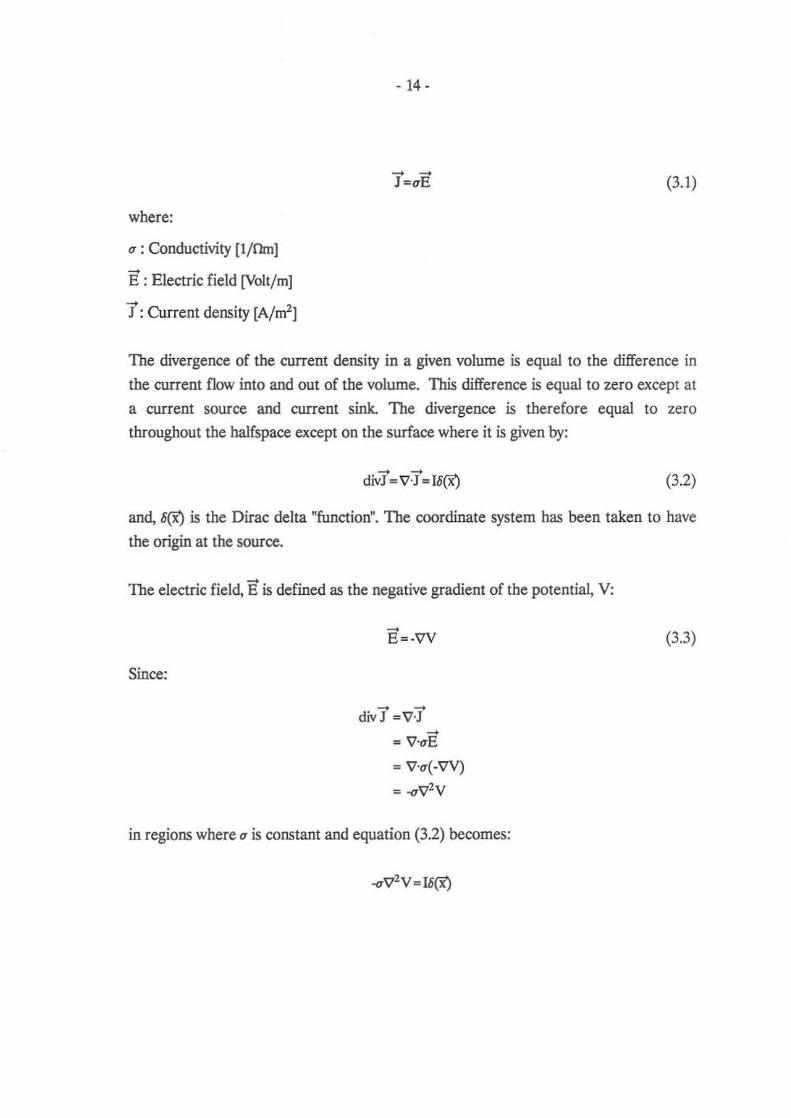
where:

u: Conductivity [l / rJrn]

E: Electric field [Volt/m]

J: Current density [A/m']

- 14-

- -}=uE (3.1)

The divergence of the current density in a given volume is equal to the difference in

the current flow into and out of the volume. 11ris difference is equal to zero except at

a current source and current sink. The divergence is therefore equal to zero

throughout the halfspace except on the surface where it is given by:

divJ= VJ= 1600 (3.2)

and, 600 is the Dirac deha "function". The coordinate system has been taken to have

the origin at the source.

The electric field, E is defined as the negative gradient of the potential, V:

Since:

-E =-VV

div1 =v1 -=V·uE

= V·u(-VV)

= ..qV2V

in regions where u is constant and equation (3.2) becomes:

(3.3)

- 15-

As u=l!p and in the uppermost layer, P=PI then:

(3.4)

Equation (3.4) is an inhomogeneous differential equation of second order. A special

solution for this equation is given by (see e.g. Hersir and Arnason, 1989):

(3.5)

where:

R= (x' +y' +z')'~

Changing from Cartesian to cylindrical coordinates, x = r·cas e, y = r·sin e and z = z

and using the identity cas'e + sin'e = 1 then:

R' = r'( cos'e+sin'e) + z' = (r' +z')

The special solution given by equation (3.5) can now be written as:

v = PI! (r' + z' )"'~ 2.-

It can be shown (see e.g. Hersir and Arnason, 1989) that:

where 10 is the Bessel function of order zero. Consequently:

PI I 00 -.\t V= - fe Io(>,r)d,\

2.- 0

(3.6)

(3.7)

This last equation is only valid for the uppermost layer where, div I = 1 6 (X'J. For all the

other layers div J = O. Therefore, for i > 1:

- 16-

or:

v'v = 0 (3.8)

Equation (3.8) is the LAPIACE equation, which can he written in Cartesian

coordinates as:

(3.9)

In cylindrical coordinates equation (3.9) becomes:

Because the layers are both homogeneous and isotropic, the potential is symmetrical

around the Z-axis, i.e. independent of O. Therefore:

a'V 1 av a'V - + - ·- + - =0 ar2 r ar az.'

(3.10)

Special solutions to this homogeneous differential equation of the second order are

found by separating the variables, i.e.:

V (r,z) = U (r) W (z) (3.11 )

Substituting (3.11) into (3.10):

Wiz) d'U(r) + WCz) dUCr) + U(r) d'WCz) = 0 d" r dr dz'

(3.12)

Dividing by U(r)W(z):

1 d'U(r) + _ 1_ dUCr) + 1 d'WCz) = 0 U(r) d" rU(r) dr WCz) dz'

(3.13)

Since U is only a function of r and W only a function of z, this can only be satisfied if:

and:

- 17 -

1 d'U(r) + _ 1_ dU(r) = _~, U(r) de' rU(r) dr

1 d'W(z) =~, W(z) dz'

(3.14)

(3.15)

Where ~ is an arbitrary constant. The general solution for equation (3.15) is given by:

W(z) = Ae!'- + Be-" (3.16)

Where A and B both are arbitrary constants. The solution for equation (3.14), which

is finite as f-O is:

U(r) = DJO(M) (3.17)

where, D is an arbitrary constant.

Since V(r,z) = U(r)-W(z) special solutions for equation (3.13) are given by the product

of equations (3.16) and (3.17), Le.:

(3.18)

Where >., ~(~) and w(~) are constants.

The general solution of the homogeneous equation within each layer is a linear

combination of the special solutions as ~ varies from 0 to 00:

~

V; = f[~;(~)e!'- + w;(~)e-1Jo(M)~ (3.19) o

for i = 1,2, ... ,n. The potential vanishes at infinity (r-->oo). The Bessel function of order

zero, JO(M) becomes zero if and only if M is a real number. Since the integrand in

equation (3.19) is symmetrical in ~ only positive values of ~ need to he considered.

The general solution for the inhomogeneous differential equation of second order in

the uppermost layer (equation 3.4» can he written as a sum of the general solution for

. 18·

the homogeneous equation (3.19) and the special solution for the inhomogeneous

equation (3.7):

(3.20)

where:

The solutions for the other layers (i > 1) can be written on the same form as equation

(3.20) by defining, for i > 1:

e,(~) = :aJ w,(~) · 1 and X;(~) = ..£..<I>,(~)

~ ~ J

The task is now to deterntine the functions e,(~) and X;(~). That is done by using the

boundary conditions for the potential, V, which are the following:

1) The potential is continuous across every boundary between layers, i.e.

V, (h,) = V," (h, ). This means that when z approaches h, from above and below the

boundary, the same potential value will be found.

2) The vertical component of the current density, 1z '" q a; is continuous across

. 1 aVj 1 aVi +1 every boundary between layers, I.e. - ~ = ----;;:- at z = h, .

Pi U£ Pi+l Vi.

3) At the surface (z=O) the vertical component of the current density (J,) is equal to

zero and consequently the electrical field also, except for a small neighbourhood

around the current source.

4) The potential vanishes at infinity, Le. V~O when Z-;oo and r..;oo.

In the lowermost layer (i =n) condition 4 requires that X.(~) = O. Hence equation

(3.20) for the lowerrnost layer becomes:

- 19-

(3.21)

Differentiating equation (3.20) with respect to z for the uppermost layer (i = 1) gives:

av, p,! 001[" " _"] - = - -Ae- -.\6,(A)e- + >.XI(A)e- Jo(Ar) eLl az 2l< 0

and on the surface z - 0 :

[aVI] p,! oo[ ] --;;;: = 2;" I -A -.\6, (A) + >.X, (A) Jo(Ar) eLl

z-o 0

For the uppermost layer condition 3 gives, J, = _1 [:] = O. Hence: PI z-o

00

I [-A -.\6, (A) + >.X,(A)] Jo(Ar) eLl = 0 o

(3.22)

Differentiating the special solution to the inhomogeneous equation, given by equations

(3.6) and (3.7), with respect to z gives:

-z (3.23)

letting z~O:

[av] p,! 00 &i = 2;" I -AIo(Ar) eLl = 0

z .. o 0

or:

00

I AJo(Ar) eLl = 0 o

Applying this result to equation (3.22) means that:

Hence for the first layer:

- 20-

00

f [XI(~) - el(~~ AJo()U) d.\ = 0 o

and equation (3.20) at the surface (z = 0) therefore becomes:

Conditions 1 and 2, at the boundaries between layers (z=h;, for i= 1,2, ... n-1), give:

and

(3.24)

(3.25)

(3.26)

(3.27)

Equations (3.26) and (3.27) constitute a system of 2(n-1) equations with 2(n-1)

unknown functions e;(~) and X;(~). Koefoed (1979) has shown how this system of

2( n-1) equations can be solved.

As an example of bow this system of equations can be solved, a simple case is taken,

the two layered model. By using equation (3.24), equation (3.20) for layer 1 at the

boundary (z=b) becomes:

For layer 2 at the boundary (z=h), remembering n=2 and using equation (3.21), the

potential is given by:

Boundary condition 1 gives:

· 21·

V1(h) = V,(h)

and therefore:

(3.28)

Taking the derivatives of the potential with respect to z, at z = h:

and:

Then the boundary condition 2 gives:

(3.29)

Solving equations (3.28) and (3.29) gives:

where:

3.2 Stefanescu's integral and the Kernel function.

The potential at the surface is given by equation (3.25). It can be rewritten as:

- 22-

(3.30)

It can be shown that for the Bessel function of order zero, Jo the following is valid (see

e.g. Hersir and Arnason, 1989):

and for z=O this becomes:

~ 1 J JO(M) eLl = -o r

Equation (3.30) can therefore be written as:

(3.31)

Equation (3.31) is a key equation, describing the potential VCr) at the surface of a

stratified medium, generated by a point current source at the surface. In equation

(3.31) the parameters involved are the following:

V : Potential at a point on the surface a distance r from the

point source

I : Current intensity at a point source

p, : Resistivity of the uppermost layer

A : Integral variable

r : Distance between the current source and potential point

JO(M): Bessel function of order zero

9, (A) : Stefanescu's Kernel function dependent on the layers parameters Pi and h;

- 23-

3.3 The Unear Filter Method

In order to evaluate the integral in equation (3.31), the socalled digital linear filter

method is used. The method is based on the theory of sampling, stating that it is

possible to reconstruct every function, F(y) completely with a finite number of

discretely sampled values taken at even intervals, fly as long as its Fourier spectrum

vanishes for frequencies higher than the Nyquist frequency, 1/2!ly. The function, F(y)

is written as a linear combination of the sample values. The coefficients in tbe linear

combination are called filter coefficients and their number the length of the filter.

The function F(y), can be written as an infinite sum:

~ sin[~(y-yo-jfly)/ fly] F(y) = jE, F(yo + jfly) w(y-yo-jfly)/ fly (3.32)

where F(y) is sampled at the points, Yo + jfly, I j I = 0.1,2, ....

By changing tbe variables y = -In(~), x = !n(r) and ~ = x - y and representing the

Kernel function, 9, (y) = 9, (~) as a linear combination according to equation (3.32), it

can be shown that equation (3.31) can be written in the following way (see e.g. Hersir

and Arnason, 1989):

(3.33)

where the filter coefficients, ~ are given as:

(3.34)

The filter coefficients depend only on x-yo-jfly i.e. the geometry of the array, but they

are independent of the layer parameters. They can therefore be calculated once and

for all and stored as numbers. VCr) is now found at points evenly distributed on a

logarithmic scale i.e. (x = X{! + ktJ.x) where ID is the interval between measured

points in a Schlumberger sounding. Choosing ID = fly and using equation (3.33):

- 24-

V(Xo + kl>y) (3.35)

Knowing the layer parameters, P;. <iJ, the Kernel function, eh can always be calculated

at the sample points by solving the system of 2(n-1) equations given in (3.26) and

(3.27). Using the result together with the filter coefficients, stored as numbers, the

potential described in equation (3.31) is easily calculated. The potential difference is

thereafter calculated by using:

!> V = 2[V(S-P)-V(S+ P)]

where:

!> V : Potential difference

S : Semidistance between current electrodes

P : Semidistance between potential electrodes

3.4 The Apparent Resistivity

(3.36)

The potential due to a point current source at the surface of an electrically

homogeneous and isotropic earth is governed by the relation:

V = A (3.37) P 211" r

Where:

Vp : Potential at point P [Volt]

P : Resistivity of the haIfspace [Om]

I : Injected current [A]

r : Distance from the point source to the point P where

the potential is considered [m]

·25·

Applying equation (3.37), it is easy to calculated the potential difference between the

potential electrodes at the surface for any combination of the current sources. In this case, Le. the tetra·electrode Scblumberger configuration, the potential difference, can

be evaluated for p, giving:

w p= -

2 S'·p2 c.v

P I (3.38)

In the reality the earth is not homogeneous and equation (3.38) no longer expresses

the true resistivity of the earth but a quantity called the APPARENT RESISTMTY,

defined as.

w P. = -

2 s'·p2 C.V

P I (3.39)

Equation (3.39) is a basic one, because it is the link between surface measurements

and subsurface resistivity distribution.

3.5 The Gradient Approach

When Scblumberger soundings are interpreted, it is often assumed that the distance

between the potential electrodes is infinitesimal compared to the distance between the

current electrodes. In this approach, often called the gradient approach, it is

furthermore assumed that the potential changes linearly between the potential

electrodes. The potential difference is found by differentiating V:

c.v = .2[aV] 2P Or ,os

This gives after some calculations (see e.g. Hersir and Amason, 1989):

~

p, = p, +2p,S' f9,(A)J,(>S)AcU o

(3.40)

- 26-

The integral is evaluated by using the filter method. The filter coefficients are though

different from those given in equation (3.34). In the gradient approach only one

integral has to be evaluated in order to calculate the apparent resistivity instead of two

for the finite electrode separation method, previously describes using equations (3.31), (3.36) and (3.39).

In fact this is the most common method for interpretation of Schlumberger soundings.

The method has the disadvantage that it does not simulate the real position of the

current and potential electrodes. This is rather cumbersome since, as will be seen in

next chapter, it brings the interpretation to an approximate solution. This is because

when p. is calculated using this approach, it always results in a continuous curve, since P is kept fixed (infinitesimal). The different segments of the P. curve will always tie in

each other, a case that hardly occurs in nature.

3.6 The Effect of Finite Electrode Separation

The depth of penetration of Schlumberger soundings, is not only a function of the

distance between the current electrodes, 2S. It is actually a function of the shortest

distance between the current electrode and the potential electrode, S-P (Arnason,

1984). For the same S and different P, different values of P. reflect different resistivity

at different depths. For instance, if the difference (S-P) in a two layer case, is of the

same order of magnitude as the depth to the layer boundary, the measured P. value

will be dominated by the resistivity of the first layer, Ph independent of the distance

between the current electrodes.

The usual procedure in carrying out a Schlumberger sounding, is to keep P as small as

possible. As S increases, I> V decreases and it becomes necessary to enlarge P. The

changes of S and P are reflected in the P. curve which is composed of shifted

segments. These shifts are convergent, because the larger (S-P) becomes, the more

the apparent resistivity values, measured with the same S, approach that of the

gradient approximation (Arnason, 1984).

- 27-

An example of a convergent shift can be seen in many of the interpreted soundings

from Planillas Geothermal Field, Mexico (see Reyes, 1989).

3.7 Sources of errors in Schlumberger soundings

In Scblumberger soundings, a current of a certain strength is injected into the earth

through a current circuit and the associated potential field is measured. It is necessary

to know the exact amount of both the current and the induced potential.

Besides the associated potential field, there are always present spurious potential

sources such as induced polarization, spontaneous polarization, telluric currents,

induction and all kinds of conductors acting as shortcut (e.g. the sea if the sounding is

close enough to the coast). It is possible to correct for the influence of the sea on the

measured P. curve (Hersir, 1988). These spurious potentials or "noise" can be handled

through statistical means. By taking many measurement values of t;. V and I, and

calculate their mean values and statistical deviations or under more difficult conditions it is possible to obtain a weighted mean-value from all the mean values were the

weighting is determined by the standard deviation in each case. Doing this the random

error will be to at least some extent averaged out.

There is another kind of effect that alIects the shape of the apparent resistivity curve

and keeps it different from a "well behaved one", which can easily be interpreted by

one dimensional interpretation. Two-dimensional resistivity distribution at the site or close to the potential electrodes can provoke a constant shift in the apparent resistivity

curve. It can easily lead the interpretation astray (Arnason, 1984). The way to handle

these shifts, is to fix the segment of the curve measured with the largest P, used in the

sounding, and correct the others by a factor that forces the segments to tie in. This is

done by assuming that the segment of the apparent resistivity curve which is measured

with the largest P, has the least local influence. This effect caused by resistivity

inhomogeneities can also be compensated for in two dimensional interpretation.

- 28-

Errors arise, when both topographic and two-dimensional effects, are erroneously

treated as being caused by a one-dimensional resistivity distribution.

Besides this, there still remains an uncertainty inherent in the method, called

equivalence. There are two types of equivalences. In both cases there is a layer whose

thickness and resistivity is undetermined. For both cases the depth to this layer's

interface, must be the same or less than the thickness of this undetermined layer, (see

e.g. Koefoed, 1979). The first one, is a bell type curve, i.e. a resistive layer which is

embedded between two conductive layers. In this case, the only known parameter for

the intermediate layer. is the transversal resistance, given by the product, Pi di "" T. The second one, is a bowl type curve, i.e. a conductive layer which is embedded

between two resistive layers. In this case, the only known parameter for the d·

intermediate layer, is the longitudinal conductance, given by the quotient - ' = SL' Pi

In tbe presence of equivalence layers in one-dimensional interpretation, it is advisable

to add some independent information from otber investigations. If they are not

available, correlations can be made utilizing other soundings in the neigbborbood.

- 29-

4. COMPUTER PROGRAMS FOR INTERPRETATION OF SCHLUMBERGER

SOUNDINGS

This chapter describes the programs applied for one- and two-dimensional

interpretation. In chapter 4.1.1 a description is given of how the gradient approach,

discussed in chapter 3.5, is applied in the PC-program SUNV. The program is a one­

dimensional automatic iterative program which evaluates tbe integral given in

equation (3.40) using the filter method. In chapter 4.1.2 the second program, named

ELUPSE is described. At Orkustofnun (NEA) it runs on either a VAX.- or HP­

mainframe. ELUPSE is also an automatic iterative program. It applies both

convergent and constant shifting, using the finite electrode separation described in

chapter 3.3 (see equations (3.31), (3.36) and (3.38». Finally, in chapter 4.2 the third

program, FEUX is introduced. FEUX is a two-dimensional finite element program

which takes the topography into account.

4.1 One·dimensional interpretation

The theory presented in chapter 3 is applied in one-dimensional interpretation. As

mentioned before, there are two methods for evaluating equation (3.31), the gradient

approach and tbe more exact one, tbe finite electrode separation method. The former

is less time consuming and was therefore implemented on a personal computer.

4.1.1 TIte gradient approach, the SUNV program

TIte SUNV program (SchLumberger INVersion) was written by Kn6tur Arnason for

tbe UNU Geothermal Training Programme. For a detailed description of the

program see Arnason and Hersir (1988). SUNV is a non-linear least-squares

inversion program using a Levenberg-Marquardt inversion algorithm together with a

fast forward routine based on the linear filter method. It automatically adjusts the

layer parameters in order to fit a calculated curve to the measured apparent resistivity

curve. In this chapter a qualitative description will be presented, to illustrate the

practical use of the program.

- 30-

In the field the potential difference, t;. V and the injected current, I are measured for

different current electrode spacing, 2S and different potential electrode spacing, 2P.

These quantities are used to construct an apparent resistivity curve. If the curve

present shifts, as commonly bappens, it must be "corrected". As already shown in

chapters 3.6 and 3.7, there are two kinds of shifts, tbe convergent and tbe constant

shift. The constant shift can be handled by fixing the segment of the curve measured

with the largest P, used in the sounding, and correct the others by a factor that forces

the segments to tie in (see chapter 3.7). This is accomplished by a manual procedure

prior to the automatic process, but there is no way to get extra information from the convergent shifts in tbis kind of interpretation. After tbis step, the corrected curve is

fed into the program. By inspection, an initial guess is made by the interpreter in order

to choose the initial layer parameters p; and d; together with the number of layers. It

is important to notice that the SUNV program although it changes the layer

parameters, does not vary the number of layers.

Using these layer parameters, the kernel function e,(A) is calculated and the

corresponding apparent resistivity values are determined by evaluating equation (3.40)

with the help of the linear filter method. The calculated curve is compared with the

measured one, and the computer changes the layer parameters until a good fit is

achieved. By inspection, the interpreter checks if the fit is good enough, if not, the

number of layers can be changed and the process reinitiated.

4.1.2 The rmite electrode separation, the ELLIPSE program

ElliPSE is a powerful mathematical program available only at Orkustofnun (NEA).

For a description of the program, see Hersir and Arnason (1989). It simulates the

actual position of the electrodes when evaluating t;. V in equation (3.36) by means of

equation (3.31). In tbis way the computer program is able to extract the information

contained in convergent type shifts, which are due to a finite potential electrode

separation and strong resistivity contrasts between layers. The constant shifts are

automatically corrected by fixing the segment of the curve measured with the largest P

and applying correction factors to the other segments so that they all tie together.

ElliPSE requires an initial guess model and by means of an iterative process the

- 31-

layer parameters are changed until a fit is achieved. The interpreter then decides if the

fit is good enough by displaying the calculated curve on the screen. The ElLIPSE

program was written by Ragnar Sigurdsson at Orkustofnun (NEA). The FOR1RAN

77 algorithm is hnplemented on a mainframe HP 9000/840, running under UNIX and

makes use of some routines from the International Mathematical Subroutines library

(IMSL). This program was used for one-dhnensional interpretation of most of the

Schlumberger soundings carried out in Planillas Geothermal Field, Mexico as is

described in cbapter 5.

4.2 'IWo-dimensional interpretation, the FELIX program

The FEUX program is a most powerful tool for two-dhnensional interpretation. It

was written by Ragnar Sigurdsson at Orkustofnun (NEA). The program makes use of

tbe finite element method to evaluate the potential distribution in a two-dimensional

resistivity distribution composed of triangular and rectangular resistivity blocks with

infinite extension in the third dhnension. The surface can be made irregular in order

to model the topography.

FEUX requires as an input, the two-dhnensional reslStlVlty distribution, the

topography and the locations of soundings along the measured profile. The program

calculates the potential distribution over all nodes in tbe net and the apparent

resistivity curves for up to ten Schlumberger soundings over the irregular landscape

along tbe profile. It 'takes into account tbe potential distortions caused by the

topography, and shnulates the actual electrode positions utilized in the field.

The calculated and measured curves are compared and the interpreter decides how to

change the block distribution, the resistivities, dhnensions or even add and eliminate

different blocks. Then tbe program is run again and the process repeated until a good

fit is obtained.

In Iceland FEUX is used for modelling resistivity data from head-on profiling and for

two-dimensional interpretation of DC-coaxial dipole soundings.

- 32-

5. INTERPRETATION OF SCHLUMBERGER SOUNDINGS FROM PLANILLAS

GEOTHERMAL FIELD, MEXICO

5.1 Introduction

A resistivity survey was carried out at Planillas rhyolitic dome and the associated area,

applying Scblumberger soundings. The purpose of this survey was to study the

subsurface resistivity distnbution, with the aim of correlating resistivity with geological

parameters, and thus get a better understanding of the rock water system connected

with the geothermal manifestations and the structural conditions in the area

As already mentioned, resistivity is directly related to effective porosity (Le. amount of

interconnected pores), temperature and water content. These parameters are of

interest in exploring gebthermai reservoirs. There are other variables that can obscure this relation, as for instance clay content, interface conduction and highly concentrated

brines.

This chapter presents a description of the results of the interpretation of the

Scblumberger soundings made during the author's training course. The facilities at

Orkustofnun (NEA) were utilized.

5.2 Geological setting

Planillas Geothermal Field is located 7 km south of Prirnavera Geothermal Area. A

regional geological survey of the Tertiary system has been executed to make clear the

structure and rock facies of the system surrounding the Prirnavera Caldera (see JICA,

1989, page 13-17). The results of this survey will be taken into account, in order to

understand the stress field causing the shallow and deep fractures and the fault system

in Planillas.

The rock formation beneath Primavera, and hence most likely in Planillas, is

composed of, in ascending order, basement granitic rocks, the Cordilleran volcanics, the Tala toff, rhyolitic domes and air fall pumice (see JICA, 1989).

- 33-

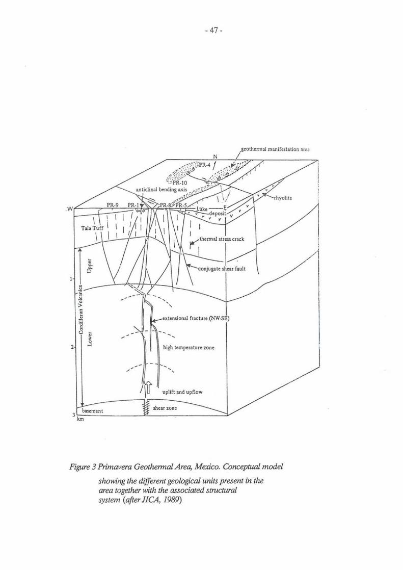
The geothermal fluids associated with Primavera Geothermal Area are mainly stored

in extensionai fractures developed within the lower Cordilleran volcanics (see figure

3). The system of extensionai fractures and strike slip faulting has a NW-SE trend.

The Tertiary formation, i.e. Cordilleran volcanics, must lie beneath the Tala tuff

formation and bave the same fracture trend below Planillas Geothermal Field as Primavera Geothermal Area

Moreover, Planillas together with Primavera is located in a point that can be

considered as "the hub of a wheel" (see nCA, 1989) with the NW-SE and E-W

trending portions of tbe Mexican Volcanic Belt, and the N-S trending Cordilleran­

Colima graben. The Colima graben seems to be a failed rift, and the Mexican

Volcanic Belt a failed transform fault. In this geological circumstance, the NW-SE or

the N-S trending fracture would be open (see figure 3).

5.3 SchJumberger soundings

5.3.1 Introduction

The Mexican Comision Federal de Electricidad, CFE, conducted a geophysical

survey, witb the author's participation, in which more than 200 Schlumherger

soundings were carried out. The location of the Sehlumberger soundings from

Planillas is shown in figure 4. They were interpreted as an integral part of the author's

training and the results are discussed in this chapter.

The Schlumberger soundings were performed using a Seintrex transmitter IPC-15,

delivering a power of IS KW nominal, 12 KW actual into the current circuit. An

analog high impedance null voltmeter Hewlett Packard was connected to the potential

circuit, with non-polarizahle potential electrodes using a CUSO, solution. The

spontaneous polarization was eliminated with an attached battery circuit and each

measurement was repeated five or six times. Thereafter the mean value was

calculated.

- 34-

The calculated apparent resistivity curves present shifting, having an overlap of five

points. These shifts were corrected manually by fixing the segment measured with the

largest P and multiplying the other segments with a multiplication factor, in order to

accomplish the input curve required for the SUNV program.

With the purpose of comparing the results from the interpretation of the SUNV

program, the soundings were also interpreted using the ElliPSE program, feeding

the computer with the actual apparent resistivity curves as obtained from the field

record. In chapter 5.3.2 the comparison is presented together with the interpretation

from the whole area, using ElliPSE. The two dimensional interpretation is presented

in chapter 5.3.3.

The measured apparent resistivity curves of all the Schlumberger soundings that were

interpreted from Planillas are published in a separate report, which is divided into

three parts (Reyes, 1989). The first two parts show the results of one-dimensional

interpretation (models, mean deviations and fits between measured and modeled

data) using the SUNV program and the ElliPSE program, respectively. The third

part shows how weU the calculated apparent resistivity curves from the two­

dimensional model fit with the measured curves.

5.3.2 One-dimensional interpretation

The Schlurnberger soundings from Planillas (for location see figure 4), were

interpreted one-dimensionally using the SUNV program and the ElliPSE program.

The mean deviations from the interpretation using ELLIPSE ranged from 3.7 for

sounding 007 and up to 19.7 for sounding 167. The average mean deviation was 10.3

(Reyes, 1989).

Two perpendicular resistivity cross sections, A-A' and B-B', oriented NE-SW and

NW-SE, respectively, were made using both SUNV and ElliPSE for comparing of

the results. The soundings interpreted with SUNV gave results close to that of

ElliPSE, a difference within 10% or less was noted between thickness and resistivity

values.

- 35-

As explained earlier in the report the difference between the models, originating from

SUNV and EUlPSE, is mostly due to high resistivity contrasts between layers. The

difference between these one-dimensional inversion techniques is demonstrated in the

next example. By looking at sounding 135 (see Reyes, 1989) it is possible to ponder,

that even though the inversion gives the same number of layers, the resulting layer

parameters are different (see table 1):

SOUNDING 13S

RESISI1VlTY [Om ] lHICKNESS [m]

SUNV EUlPSE SUNV EUlPSE

1204 1847 2.8 5.7

5556 4759 183.9 183.0

281 113 1835.2 221.0

11661 356

Table 1 Inversion models for sounding 135, SUNV and

ElliPSE inversion

Inspecting the shallow part of the curve, a shift is noticed between the segment of the

curve measured with P = 2.5 m and with P = 10.0 m. The latter segment has higher p,

values than the former segment, as expected, because of the ratio between layer

resistivities, />2 / PI = 2.5. The program SUNV can not handle the shift because it is not

fed into the program. The "corrected" continuous curve fed to SUNV, depends on the

interpreter criteria

Prior to interpretation of sounding 135 by SUNV, it was manually "corrected", by

lifting all the segment measured with P = 2.5 m, until it tied in with the segment

measured with P = 10.0 ffi.

In this case, the model from SUNV has higher resistivity values for the second layer

than ElliPSE. Sounding 135 is particularly troublesome in the deeper part. The

measured P. values spread a lot. Both programs take the best fitted curve, in the

least-squares sense, but EUlPSE is able to model the shifts.

- 36-

Table 2 shows the comparison for sounding 185, a curve almost without shifting (see

Reyes, 1989):

SOUNDING 185

RESISTIVI1Y [ Om ] lHICKNESS [m]

SUNV ElliPSE SUNV ElliPSE

823 997 1.6 1.9

238766 19332 2_6 2_8

3175 3666 121 102

263 356 332 291

15 14.5 705 587

110 71

Table 2 Inversion models for sounding 185, SUNV and

ElliPSE inversion

From table 2 it can be deduced, that the two resulting models are practically the same,

as could be expected, since sounding 185 presents almost no shifting_

Although there is a marked difference between the models originating from the

inversion using SUNV and ElliPSE, respectively, it is interesting to note that they

give very similar resistivity distribution_ This tells, that even in extreme cases (high

resistivity contrasts between layers, like sounding 135) SUNV gives sufficient results if

the data are treated "correctly" prior to the inversion_

Two resistivity cross sections were made. Their location is shown in figure 4. Cross section A-A' runs NE-SW along Cerros Las Planillas rhyolitic dome, from Agua

Caliente to La Cebada_ Section B-B' crosses A-A' almost perpendicularly close to the

steam vents, which are found at a relatively high elevation (2200 m a.s.!.). Two iso­

resistivity maps were made, showing resistivity distribution at two different levels,

1.500 and 1.000 m a.s.l. Here, resistivity cross sections and iso-resistivity maps will be

described.

- 37 -

Both cross sections were made using SUNV (see figure 5 and figure 7) and EUlPSE

(see figure 6 and 8), respectively. Each pair looks quite similar. Therefore for practical

purposes only the EUlPSE inversion will be discussed. The iso-resistivity maps were

drawn according to the results from the EUlPSE inversion.

Resistivity cross section A-I< (figure 6) crosses Cerros Las Planillas rhyolitic dome

from SW to NE. It includes 13 soundings with half the current electrode spacing (S)

ranging from 40 up to 3.000 m. The surface layers have a thickness around 150 m and

a resistivity of about 1.500 Om or higher. This must correspond to the rhyolites and the

dry part of the Tala Tuft.

Beneath the surface layers there is a layer with resistivity of 100-1.500 Om which must

correspond to partially saturated rocks, witb high resistivity water or low porosity

layers mainly belonging to the upper Cordilleran volcanics (lithic tuft). Below these

layers there is a resistivity low, stretching to the east and to the west as far as the cross

section has been drawn.

At both the western and the eastern branch of the profile tbere is a resistivity high

beneath the resistivity low. Between soundings 004 and 152, higher resistivity beneath

the resistivity low is not found. Below sounding 162 there is a structure characterized

by resistivity values of 100-1.500 Om. It might reflect an impermeable barrier.

Resistivity cross section B-B' (figure 8) runs from NW to SE. It includes 9 soundings

and presents the same high resistivity surface layers as cross section A-I<. They must

correspond to the surface rbyolites and the dry Tala tuft formations. The second series

of layers, of 100-1.500 Om resistivity values, must correspond mainly to the lithic tuff

(upper Cordilleran). The extension of the low resistivity is well defined by relatively

resistive structures at both sides, NW and SE.

The general picture of the resistivity structure at Planillas Geothermal Field, Mexico

is shown on two iso-resistivity maps. Figure 9 shows the resistivity at 1.500 m a.s.l. and

figure 10 shows the resistivity at 1.000 m a.s.l. The figures show the location of the hot

springs and the steam vents as well.

- 38-

Figure 9 shows a low resistivity, described by the 40 Om contour line. It presents a

NW-SE trend. The 30 and 20 Om contour lines have the same trend. Outside this

anomaly the resistivity increases. They are not well defined though. In figure 10, the

20 Om contour line presents the same trend, NW-SE. But it also has a mixed trend,

running N-S. Outside this anomaly the resistivity increases.

Figure 11 shows a division of PlanilIas Geothermal Field into resistivity zones,

depending on three different categories of soundings. These categories are: The

resistive or ascending type (resistivity higher than 40 Om at depth), the conductive or

descending type (resistivity less than 40 Om at depth) and the higher resistivity below

the low resistivity or bowl type.

The division shows the general resistivity distribution but more importantly it suggests

a probable flow mechanism of the geothermal fluids in the area.

The conductive zone is flanked to the east and to the west by resistive zones and at some parts there is a bowl type zone, at the intersection between the resistive and

conductive zones. This could be explained as being due to flow of geothermal fluids

ascending within the limits of the conductive zone and laterally leaking into the bowl

type zone. The resistive zone could be caused by low porosity or lower temperatures.

5.3.3 'l\ro-dimensional interpretation

Profile A-~ (for location see figure 4) was interpreted two-dimensionally, taking the

topography into account. In two-dimensional interpretation the resistivity is assumed

to change both with depth and in the direction of the profile but not perpendicular to

it. Two-dimensional interpretation is described in chapter 4.2.

The profile consists of 10 soundings, all of them laying parallel to the profile. The

resistivity cross section resulting from the one dimensional interpretation (see figure

6) was used as a starting model for the two-dimensional interpretation. After the

model had been changed several times, an acceptable model was found. It is is shown

in figure 12. The location of the soundings, the hot springs and the steam vents are

- 39-

shown as well. The curves for the calculated and measured apparent resistivity are

published in a separate report (Reyes. 1989). They show how well the model data fits

with the measured date for each sounding.

The general distribution of resistivity is different from the one-dimensional case in

many ways. For instance, the influence on neighbouring soundings is taken into

account in the two-dimensional program. The apparent resistivity curve of some

soundings shows a low resistivity mainly caused by their vicinity to low resistivity

rather than the resistivity structure beneath them. The resistivity values resulting from

one-dimensional interpretation seem in some cases to be overestimated and a

narrower low resistivity distribution better defined between soundings 158 and 161 is

revealed by the two-dimensional modelling.

The two-dimensional model is characterized by a resistivity low of resistivity less than

15 nm and 3.5 km wide in the southwestern slopes of Cerros Las Planillas. This main

anomaly is narrower and better defined than in the one-dimensional model. It is

bordered by a resistivity high on both sides. To the east and to the west of this anomaly

there is a low resistivity. having higher resistivity beneatb tbe low resistivity. Inside the

main low resistivity anomaly there is a narrower anomaly. 1.2 km wide and having a

resistivity of 7 Om.

At the eastern border of the main anomaly. there are steam vents at a relatively high

elevation suggesting that the ascending path of this steam is stretched by the border

between high and low resistivity values. At the western border of the main anomaly.

there are hot springs at a relatively low elevation suggesting a near vertical convection cell.

Application of the FEUX program for two-dimensional interpretation of profile A-N

results in a more clear picture of the resistivity distribution with both depth and

horizontal direction.

- 40-

5.4 Results

One-dimensional interpretation of Schlwnberger soundings from Planillas

Geothermal Field indicates a low subsurface resistivity anomaly (resistivity less than

40 Om). At 1.500 m a.s.!. the anomaly presents a NW-SE trend. It continues at greater

depths (1.000 m a.s.l.) with the same NW-SW trend together with an additional mixed

N-S trend having lower resistivity values (less than 20 Om).

The geothermal fluids associated with Primavera Geothermal Area are stored in

extensional strike slip faults with NW-SE orientation, within the lower Cordilleran

volcanics (andesites), reactivated and opened by a vertical stress field. Primavera

Geothermal Area is located 7 km north of Planillas Geothermal Field. The same

geological formations, i.e. lower Cordilleran volcanics are located beneath Planillas

Geothermal Field. Two-dimensional interpretation of a profile perpendicular to the

low resistivity anomaly suggests an over estimation of the resistivity values in the one­

dimensional interpretation, due to lateral and topographic effects. The two­

dimensional interpretation is characterized by a less than 15 Om anomaly, 3.5 km wide

in the southwestern slopes of Las Planillas flanked by two relatively resistive

structures, reaching towards the surface. At the NE flank there are steam vents and

near the SW flank hot springs are found, at a relatively low elevation. Inside this main anomaly there is a narrower anomaly. 1.2 km wide having a resistivity of 7 Om. This

suggests a possible vertical flow of geothermal fluids in the middle of the low

resistivity anomaly probably convecting along an open fault oriented NW-SE within

the lower Cordilleran volcanics and leaking laterally SW and NE into the upper

Cordilleran volcanics (lithic ruffs).

The interpretation of Schlwnberger soundings from Planillas Geothermal Field has

proved to be of great importance in the understanding of the geothermal field. It has

also showed that one-dimensional interpretation is not adequate. Two-dimensional interpretation is necessary where the rugged terrain of the area is taken into account.

For that purpose more Schlurnberger soundings are needed. They ought to be densely

spaced (of no more than 500 m between soundings) and oriented along profiles, both

parallel and perpendicular to the resistivity anomaly. It is quite possible that the much

less time consuming and less expensive Transient Electromagnetic Method (TEM)

could give the information needed on the resistivity distribution.

- 41-

6_ CONCLUSION

The depth of penetration of Schlumberger soundings is controlled by the shortest

distance between the current electrode and the potential electrode (S-P). This

together with the actual use of the finite potential electrodes separation over a

resistivity distribution with high contrasts between layers and lateral resistivity

variations near the surface at the sounding site, causes converging and constant shifts of the different segments of the apparent resistivity curve. These shifts, if not correctly

treated will lead the interpretation astray. The theory of one-dimensional

interpretation of Schlumberger soundings is presented in this report in some detail to

understand the reasons for these shifts and to make an appropriate use of two

computer programs for one·dimensional interpretation. A two-dimensional

interpretation program, which takes the topography into account, is also discussed.

One-dimensional interpretation of Schlumberger soundings from PlaniIlas

Geothermal Field indicates a low subsurface resistivity anomaly. Two-dimensional

interpretation of a profile perpendicular to the low resistivity anomaly is characterized

by a less than 15 Om anomaly, 3.5 km wide in the southwestern slopes of Las Planillas

flanked by two relatively resistive structures, reaching towards the surface. At the NE

flank there are steam vents and near the SW flank hot springs are found, at a relatively

low elevation. Inside this main anomaly there is a narrower anomaly, 1.2 km wide

having a resistivity of 7 Om. This suggests a possible vertical flow of geothermal fluids

in the middle of the low resistivity anomaly probably convecting along an open fault

oriented NW-SE within the lower Cordilleran volcanics and leaking laterally SW and

NE into the upper Cordilleran volcanics (lithic tuffs).

The interpretation of Schlumberger soundings from Planillas Geothermal Field has

proved to be of great importance in the understanding of the geothermal field. A

more detailed resistivity survey of the area is suggested. This could either be densely

spaced Schlumberger soundings, oriented along profiles and interpreted two­

dimensionally taking the rugged terrain into account. Or possibly the much less time

consuming and less expensive 11-ansient Electromagnetic Method (TEM).

- 42-

ACKNOWLEDGEMENT

The author wants to express his profound gratitude to his advisor Gylfi PaIl Hersir for

his unselfish and unwearied support during the whole training programme. Many

tbanks go also to Kniitur Arnason both for reviewing this manuscript and for writing

the SUNV program and for his donation to UNU fellows. Dr. Ingvar Birgir

Fridleifsson is thanked for organizing the programme. The author is indebted to Ing.

Miguel Ramirez G. and Ing. Antonio Razo M. for their intervention to allow him to

participate in this important training.

- 43-

REFERENCES

Archie, G.E., 1942: The Electrical Resistivity Log as an Aid in Determining some

Reservoir Characteristics. Tran. AIME, 146, pp 54-67.

Arnason, K, 1984: The Effect of Finite Potential Electrode Separation of

Schlumherger Soundings. 54th Annual International SEG Meeting, Atlanta, Extended

abstracts, pp 129-132.

Arnason, K , 1989: Central Loop Transient Electromagnetic Soundings Over a

Horizontally Layered Earth. National Energy Authority of Iceland. OS-89032/ JHD-

06, 129 p.

Arnason, K and Hersir, G.P., 1988: One Dimensional Inversion of Schlumberger

Resistivity Soundings. Computer Program Description and User's Guide. UNU

Geothermal Training Programme, Report 8, 59 p.

Arnason, K and Hersir, G.P., 1989: Geophysical survey at Nesjavellir high­

temperature area SW-Iceland. Manuscript.

Caldwell, G., Pearson, C. and Zayadi, H., 1986: Resistivity of Rocks in Geothermal

Systems: A Laboratory Study. Proc. 8th Geothermal Workshop, pp 227-231.

Dakhnov, V.N., 1962: Geophysical Well Logging, Q. Colo. Sch. Mines, 57 (2), 445 p.

Fl6venz, 6 .G., 1984: Application of the Head-on Resistivity Profiling Method in

Geothermal Exploration. Geothermal Resources Council, Transactions. VD!. 8, pp

493-498.

Fl6venz, 6.G., Georgsson, LS. and Arnason, K, 1985: Resistivity Structure of the

Upper Crust in Iceland. Journal of geophysical research. Vo!.9O, no.BI2, pp. 10,136-

10,150.

- 44-

Hersir, G.P., 1988: Correcting for the Coastal Effect on the Apparent Resistivity of

Schlumberger Soundings. Orkustofnun OS-88O 19/JHD-10 B, 13 p.

Hersir, G.P., 1989: Geophysical Methods in Geotherrnal Exploration. UNU

Geothermal Training Programme.

Hersir, G.P. and Arnason K, 1989: Schlumberger Soundings Over a Horizontally

Stratified Earth. Theory, instrumentation and user's guide to the computer program

EWPSE. UNU Geotherrnal Training Programme.

JICA, 1988: La Primavera Geotherrnal Development Project in Mex;can United

States, final report. Japan international cooperation agency.

Koefoed, 0., 1979: Geosounding Principles 1, Resistivity sounding measurements.

Elsevier Scientific Publishing Company.

Reyes, V.P., 1988: Resistivity, Induced Polarization, Gravimetry and Magnetometry

applied on Los Negritos, Mich. Geotermia, revista mexicana de geoenergia Vol 4 no.

3, 211 p. In Spanish.

Reyes, V.P., 1989: Appendices to the report: Resistivity methods with application to

Planillas Geothermal Field, Mexico. UNU Geothermal Training Programme.

Stefansson, V., G. Axelsson and O. Sigurdsson, 1982: Resistivity Logging of Fractured

Basalts. In: Proceedings of Eight Workshop Geothermal Reservoir Engineering,

Stanford University, Stanford Calif., pp 189-195.

- 45-

A M v

N

p

p

~C > 40A

Figure 1 Sch/umberger arrangement and Head-on configurations

The uppermost figure shows the Schlumberger configuration while the lowermost one shows the Head-on configuration

c

(rn) - 5OQ.. , , , , ... ---RhO IOhrnrn) ,

AB ,

'50

'00

-500

o

100

-500

- 500

, o

20

o

- 46 -

, , "-- -- -

100

, , ,

- - RhO Ae -AB

- - - Rho ae-AB

IOhmrn)

,0

, o

-,0

, ,.. Irn)

Figure 2 Head-on profiling over conductive vertical structure

- 47 -

N /seOthermll manifestation ~I ~a

basement 'km

conjupte shear fault

high temperature 'Zone

uplift and upnow

shear :tone

rhyollte

Figure 3 Primavera Geothermal Area, Mexico. ConceplUlll model

showing the different geological units present in the area together with the associaJed structural system (after JICA, 1989)

- 48-

Figure 4 Location map of Schlumberger soundings at Ploni/las

Geothermal Field, Mexico

i

i ! •

i

i f J

~

- 49 -

E W ~ Z

~

<t:~ § <::J -'" 0 .2 §I

(I) ~ 'i7i :;0' ....I :is !:: - 0 ,2 Z .... iij 5 r.l'ij Q. ~ a. • ~~ ._ c § 0·-

·0 , ~~

I • §

~ : !i I .§ ,-

0 i B 0 ~

I • • •

!ill

! I; i\ ~9 ., , I. , i i i i i , , i i ,

rE 1 ~ ~ ~ ~ ~ ~ ~ § § ~ ~ 0 ~ ~

Figure 5 Resistivity cross section A-A " l-D SLINV-inversion

- 50-

w ,

z ~

~

W

<'" ~ <~ c ~ OW • ;g>

:I ~" • 0

=~§ z e .-S 0 i5 ~ -

~ ~i ~

~~ ~ I ~ ~

• g • I .1 j -

i 10 0 8

~

11 !§

• ,

[J

I I' ~ i h ; , , , , , , , , , , , , , ,

0 ~~ ~ ~ ~ ~ ~ ~ § ~ ~ ~ • ~ ~

Figure 6 Resistivity cross section A-A; J-D ELliPSE-inversion

- 51-

•••

o

:-:

.. :: ,

I

j j j j j j j j j j j

~ ~ ~ ~ ~ ~ § ~ § o ~ ~

Figure 7 Resistivity cross sectionB-B; J-D SUNV-inversion

- 52 -

'I' ,

.1:

l ::: i

,

!i

, :-:

•• • ••

, , ,

:j ••• , ::

o

, :: ,

, , ,

,

::: ,

• . ~ ~~ ;;: .. z · 0 " ~2;

~~ I I I I I I I I I I •• ~ ~ ~ § ~ ~ ~ ~ § ~ ~ ~

0

E

Figure 8 Resistivity cross section B-B; J-D ELLIPSE-inversion

cS - 53 -

~ cS c ~ 2 E

- c -J~ j is m

;1 eo c

f! f i~ ~ .§' III liE .2~ ~ ~

0 H ~~ S2 ~ ~ Z W

§ 0 • ~ -W--.'

• •

•

Figure 9 Iso-resistivity map at 1.500 m a.s.I.

- 54-

Figure 10 Iso-resistivity map at 1.000 m as.L

LEGEND

t '" o Low resistivity, .V' less than 40 ()n

'" - fW H~her resistivity .... '\' ......... · be ow low resistivity :... 'V 01 .. 11 High resistivity, higher a ' . than 400m

.!;l, • Schlumberger "'- 'to 149 sounding nr. 149 :§i '" '" & Steam vents 01 'tI i'. '. :4f Hot spring 01 .. ..,

'" c;. "'.

1" ~ \ - 0 500 1DOOm ~ ~.

, , , V> '\' 'to V>

n ' to ' \' E\ & ~ &A" " 'I' ~. ~

'¥ 'to '¥

'¥

'¥ 'l' . '. '1' '," '.

t '" ..... '" ~ " "­§ ~ [ " ~ 1:; -

~­~-

'" & '" ~ ~ .g, ~ :.. :i..

~ JHD HSI> !lOO:) MA ~ 89.10.0545 OoIT

m.as.!. sw 2400

2100

1800

1500 1500

1200 -

900

600 200

300

• .JOO -,

500

...,.

'r I

15

20

400

PLANILLAS

Resistivity cross-section A-A' 2-D interpretation

Crossing section 8-B' Steam vents 1'61

:""~V~--l";" ,. '. l' 0' ~ 2500 9000 I ~ .i ~ ~ 800 1 4000

L-- 50 30 5500 350 .00---100 ~

V 1500 14 15 13 100 ,.

200 15 7 500 12 75

Q , 1spa , 500 2500 m

1500

•

100

NE

V> 0,

1989

APPENDICES TO THE REPORT: RESISTIVTIY METHODS WITH APPLICATION TO PLANILLAS GEOTHERMAL FIELD, MEXICO

Pablo Reyes Vermot UNU Geothermal Training Programme National Energy Authority Grensasvegur 9 108 Reykkjavfk ICElAND

Permanent Actress: Comision Federal de Eleetricidad Superintendeneia General La Primavera Km. 21 +460 Periferieo Norte Cd. Granja Zapopan, J aliseo MEXICO

- 3-

These are the appendices to the report: Resistivity methods with application to

Planillas Geothermal Field, Mexico: It was written by Pablo Reyes Vermot at the

UNU Geothermal Training Programme in 1989. It is divided into three parts. The

first two parts show the results of one dimensional interpretation (models, mean

deviations and fits between measured and modelled data) using the SUNV program

and the EUlPSE program, respectively. The third part shows how well the calculated

apparent resistivity curves from the two dimensional model (see figure 12 in the main

report) fit with the measured curves.

- 4-

- 5 -

APPENDIX I

One dimensional interpretation of Schlumberger soundings.

SLINV-program:

Models, corresponding calculated apparent resistivity curves (shown as continuous curves) and measured apparent resistivity curves (shown as points).

- 6-

~

E E .c o ~

o o .c 0:

10 •

10 •

10

10 •

O·

0'

.......,

10

I

STATION:

•

10

STATION:

004 4 LAYERED MODEL

029

Layer ",0 d 1 1318.2 25.' , 84.9 210.3 , 348.8 183.9 , 111.9

CIIiaq _ .0'90

\ "-

10' A3/2 (rn)

-

I~

, 10·

4 LAYERED MODEL ..,... ",0 d I 46.9 ., , 4033.8 1851.51 , 422.7 318.8

/ llq _ .014 ~8.1

(

10

L---\

I

\

10 ' AB/2 (m)

10'

I " 10

10

· 7·

~

E E .c o

10 •

10 •

........ '0 2

o o .c 0:

~

E E .c

10

10 •

10 '

o '-'10· o o .c 0:

10

STAnON: 01 5 LAYERED MODE!. ..,., ",0 d

I 117.0 1.0 , 900.7 , ... J 16:373.8 11.9 , 193.5 507.11 , 12.2

Q\l8q - . Hi2

• ,.....

'\ I 1\

'0 10 ' AB/2 (m)

10 '

STATION: 135

• V

, , 10

4 LAYERED MODEl. ..,... ",0

1 1203.8 Jr 2 5556.1 1 .9

~;'71' .. , ... 681.8.1

3< _ .1

\ • • .<

•

'0 • ta/2 (m)

'0 '

,0

'0

'0 •

, 0 '

1

10

'0 •

'0'

'0

STATION -r. 2 5 LAYERED ~ODEL Lo,,, "" d

...... , .5414.5 ,., 2 19004.5 13.5

\ l 2339.5 145.5 634.4 285.6

~ 37.2 DCh~ ... 141

\ 1\

\" •

' 0 10 ' AB/2 Cm)

'0 '

STATION:_157

'0

6 LAYERED MODEL

", .. "" d , 1470.4 7.2 2 14<t.6 2.0 J 13362.2 6.0 , 94.6 682.2 5 30.0 610.6 6 981.1

"" .. .0711

i\

'0 ' MJ!2 (m)

'0 '

'0

'0

- 8-

~

E E .c

'0 •

'0 '

o --10 2

o o .c

'" '0

'0 •

'0'

'0

STATION: 156 6 LAYERED MODEL

V •

' 0

STATION: 158

, '0

Loyo, "" d , "J '.0

2 9501.3 5.' J 10.7 41 .2 , 477.8 !lS,3 5 16.0 1342.5 6 oi'S.S

... 144

~

\ . •

;0:

, 0 ' AS/2 Cm)

'0'

5 LAYERED MODEL

Loyo' "', d

1 "202.5 2.0 pro 10' 6258.2 150.0

108.5 279.2 5 0 23.7

iaq .. . 088

\ 1\

, ' 0 '

A3/2 Cm ) ' 0 '

' 0

'0

~

E E " o

10 •

10'

"-" 1 0 • c o " 0:

~

E E " o

10

10 •

10 '

'-'10 • c o " 0:

10

STATION 159 5 LAYERED MODEL loyer "" d , 212.5 1.0

~ 2 32590.7 8.0

/ " 322.1 332.6 K '23'.4 99.' (

10

STATION:

10

21.6 OIl.'! .. . 102

\ 1\

1\. •

10 ' AB/2 (m)

10'

[TOT

V

-4 LAYERED MODEl

Coy~ "" d ~ 2447.1 12.7

8002.4 28.7

10 • "'/2 (m)

1~4 "" " 35.9 Chl ... 061

\

10 '

10

10

-9-

~

E E " o

10

10

~10

o o " 0:

STATION: •

,~ r

•

10

10

160 -4 LAYERED MODEL ...,., "', d , lJ~.l , .• , 3138.3 47.5 3 10~.8 339.9 4 17.7

I ~ CIIIaq" .070

f\ 1\

\

10 • MJ/2 (m)

10 '

STATION: 162 5 LAYERED MODEL

10 •

I.

10 '

10

10

Coy., 'h' d , 2367.7 •. , , 4733.5 ••• 3 3016.6 203.4 863.2 1111.S

~7 Ch ... 080

10 • A9/2 (m)

\ •

10 '

10

., 10

STATION: 164 10'

1

10 '

10 ~

1 10

4 LAYERED MODEL

Coy" "', , 1 2525.S 21,9 2 12454.5 ,., J 1792.2 24J.1 ... 24.9

"""'" CIlia<;" .064

10 • AS/2 Cm)

......

\ 1\

10'

! i I . ,I p,ATIO~ : 166

'~l ll~'= 6 L'WERED MOCEL

I Lcyer rho

- I ' I

I I 1i ' ~ 0 •

i O .:

, U I' -

llJ , ' I , ' , , I

I --

I I 1 I - I , , 1

I 1 I

• I I I

10 I

I 1 ~a4.2 "\J ~ !2740.~

~ 0 ' '' .•

lA a.~ 0 .0

aa.l 120.6

...

I -+ 67i .l;.5 ~~J5.2

0/5' · _~29.1 Ch';!!! ... 122

'I

l '--- I. , I I \ , ,

I

1 :eo ! ,

, "

•• 11 .. I . 10 . 10 ' AB/2 Cm)

10

, ,

1 . !

! j

I I 1 ,

.I

. 10·

10

J ~

E E

cS ~1

o o & ]

~

E E .c

1

10 •

10 '

o '"-'10 • o o .c 0:

10

J , J

1

I 1

1 1

I 3

1 1 ,

1 ,

STATI N: 165 4- LAYERED MODEL 19yer "', ,

1 327.7 .7 ~ 2 21228.1 •• S

•

10

STATION: 167

-

0

•

- ,

. ,. ... , 10

• .. ~J9.J 235.7 39.0

"'" .. . 1:38

\

10' A3/2 Cm)

\

\. I

10'

6 LAYERED MODEL l.o,u m. ,

1 115.5 ., 2 5090.9 J.' J 13.3.7 '.S 4 6933.J 18.3 5 278.6 401,0 . ' I ••

18.6 Ch;. .. .1gS

"'1 '\'\l

1\. I I

I

10

! I . I ...I , .. , , , ,,5,

10 ' ;'3/2 (~)

10 ' 10

~

E E .c

10

10

o ~10

o o .c

'"

~

E E .c

10

10

10

o ~10

o o .c

'"

•

,

,

,1

.

, l

1 .1 i j

10 1 1 j

STATION:

•

10

STATION:

168 4 LAYERED MODEL

""" "" d , 298.3 .. , I • , 6129.0 23.1 , 2521.3 23.5.2

• 21.7 O~_.I.Jl

\

J\. •

10 ' AB/2 (m)

10 '

170 4- LAYERED MODEL

"'~ "" d , 24.9 .. 0 2. 127JUl IS.4 , 466.7 516.9

• 194.4 Chisq _ .1l95

,y -;-"

/' "- .. ,v ~

... . , , 10 1 0 '

10

10

. 11·

, , ]lpS~T~A~T~IO~N~':f~l ~6:9:::t~'rL~,yriEiR~EO~'~'0;D~E"'L-10'. CD,.. "'. d

i I P 1 1068.0 2.! ? 7:;10.6 21.e

1 , 1'\'\l:i '''., i I c:~ - .m

10 ""l-L----j--_!-+I ----'\\--r-__ _

I 1 I 1 \1 2.

'0 ,,..J. __ -+1 __ +-+-_+\}\ __

c c .c

'"

I I "t

j 11 i\.· j !. •

lC~J---+---~---+--~ j

~

E E .c

10

10

o ~10

o o .c

'" 10

J

j

•

,

,

. , ..... , .. It ... , ,. ".11 , iO ' "ic' '0 10

STATION: 172

V •

, 10

.~./2 (m)

5 LAYERED MODEL

Layer "" d 1 50.4 .9 , 4981.6 13.15 , 1420.3 1711.1 • 26.1 1492.6

10 ' 1>3/2 (rn)

5 136.7 Chit'l- .077

\ ]\ V-

, 10 ' 10

~

E E

10

10

..c o ~10

o o

..c

'" 10

r-TArpN:

•

,

,

10

185 6' LAYERED MODEL

"'" "', , 1 822.9 L'

0 2 23876.8 2.' , 3175.3 121.0 1'\ 263.1 332.5

1S.0 705.1 110.5

Ch!. ... 050

10' /oS/2 (m)

~ ~

10 ' 10

- 12-

~

E E ..c

10

10

o ~10

o o

..c

'" 10

STATION: •

,

,

1

10

187 4 LAYERED MODEl

"'" "', ,

V

10 ' >3/2 (m)

1 269.1 17.e 2 1293.0 168.2 , i.O 1117.0 • 223.2

CI\'-q .. .0511

\ ~

, 10 ' 10

· 13·

APPENDIXII

One dimensional interpretation of Schlumberger soundings.

ELLIPSE-program:

Models, corresponding calculated apparent resistivity curves (shown as continuous curves) and measured apparent resistivity curves (shown as points).

· 14·

- 15-

'HI.

RESISTIVITY

~ ~ ~ ~ ~ ~

" > > ~ ~ • • • • ID ID

" " ~ ~

c C ID ID

" " • • "- 0. 0. 0. « «

. . • • . . A8/2 [m } A8/2 [m)

SOUNDING SOUNDING

E E c c

~ ~ ~ ~

> > " " ~ ~

• • • • ID ID L " ~ ~

c C ID ID

" " • • 0. 0. 0. 0. « "

" ... • • t! . . A8/2 (mJ A8/2 [m}

- 16-

RESISTIVITY

E c

~ w

w W

W ID L

C ID L • Q Q « , .

.. . . • I 'j . ..: . . . . A8/2 (m l A8/2 ImJ

i=lESISTIVITY

E E C C

~ ~ w w

> > w w • • • • ID ID L L

w w C C ID ID L L • • Q Q Q Q « «

. . . . • I 1I . . . . . . . . A8/2 Im) AB/2 (m)

- 17 -

'9lIi .

!VITY SOUNDING SOUNDING

, ,~ . 'i. .1.0 ... E E C C

> > ~ ~

" ~ ~

" " ." " " • ~ L

L 0 0. 0. ~

. . . . A8/2 [m] A8/2 [ml

,sal .

RES I STIVITY SOUNDING SOUND!NG

e c

. . • • . . . . AE/2 [mj A8/2 {m l

e oS ~ ~

» ~

m ." m • c ~

c • c • a a .,

> ~

. .

" .e. 17.1 ""

. . A8/2 Im)

SOUNDING

>.!i--+~~+=~~~

.. . . . . . . A8/2 [m)

- 18 -

.-SOUNDING

e c

> ~

> ~

m m • .. c ~

c • c • " a .,

.. • • . . A8/2 [m)

!VITY SOUNDING

.. . . . . • • A8/2 {m]

. 19·

, .. ,.,. I TY SOUNO I NG RESI STIVITY SOUNDING

E E

'" C

~ ~ ~ ~

~ ~

• • • • 0 0 C C

C C 0 0 C c ro ro a a a a

" .,

, .

. . . . . . • • AB/2 (mJ A9/2 101

RESIST

" E C

~ ~. ~ ~

> ~ ~ • • • • 0 0 c c

~,

c 0 c ro a a .,

.. . . •• . . , . AS/2 [m) ABle: [m]

- 20-

RESISTIVITY SOUNDING

E E 2- c

> > ~ ~

" " ~ ~

• • • • ID ID L L

~,

C C ID ID L L

• • Cl Cl Cl Cl

'" '"

" . . . . . . , .. AS/2 [m J A8/2 [m J

RESISTIVITY SOUNDING

E E 2- 2-> > ~ ~

> , > " ~ ~ • • • • ID ID L L

~ ~ c C ID ID L L • • Cl Cl a a

'" '"

. . .. . . . . • • • • 11 . . AS/2 (m) AB/2 [m]

RESISTIVITY

E C

~,

~

~

" " • C

C • c m a a ~

• ,. $ . . . . . . AB/2 Iml

RESISTIVITY SOUNDING

.••• 253".

~,,~-------+-------+---4---+~-----c • c m a a

~,,~----~~----+-----~----~

AB/2 Iml

- 21 -

RESISTIVITY "

E C

~ ~

~

"

. . . . • I.' . . A8/2 Iml

RESISTIVITY SOUNDING

A8/2 Iml

,M' SOUNDING

E c

f,;t====:f-----bb:H-~ ~

m

m • L

E C

~ ~

" ~ --" -• L

~

C • L 0

" " <

.. AB/2 (m)

,-RESISTIVITY SOUNDING

. . A8/2 (mJ

·22-

hESIST!VITY SOUNDING

11 109 , " . 0)1) '"

A9/2 [ml

RE5IST!V!iY

E C

~ ~

>

~

" m • L

A8/2 [m)

E E > ~

> ., " " • " ~

c • " • a a ~

c • " • a a ~

SOUNDING

, . , . A8/2 [m]

RESIST I VITY SOUNOI~~

A8/2 [m]

- 23-

.. c

>. ~

> ~

" " • " ~

c • " • a a <

, . . , . .

,A'. RESISTIVITY

.. • '" • >- H .O ....

, . , . , . . , . A8/2 [m]

SOUNDING

• 16\1 13 • ...

, . A8/2 [m ]

,., ~ESISTIVITY SOUNDING

6 >-~

> ~

0

" 0 • c ~

c • c ro n n 4

. . : AB/2 [mJ

108 ;,,,:~ ,-

• ,

r-

E • S · >-, '\ ~

" .'; : 0 . " ~ • , c

;:

f : ,

, , . • i,'o • , , • Iluf •

A8/2 ImJ

,,3~

"

\ ~

I I . " ,

. .

. ..

- 24-

E c

>-~

> ~

0

~ • c ~

c • c ro n n .,

E C

'lieD.

RESISTIVITY SOUNDING

• ' . . 11 • 7. 3 00

. . AB/2 {m]

' ,,"~ .

SOUNDING

. .., A8/2 Iml

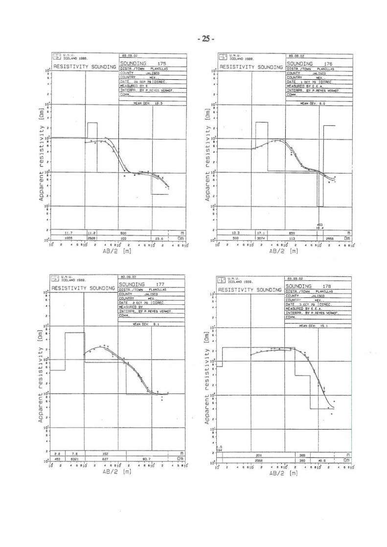
- 25-

SOUNDING RESISTIVITY

~ ~ > > ~ ~

> ~ ~

m m m m • • L L

~

C C • • L L m m Q Q Q Q ., .,

. . , . . .. . . .. . . .. . . Aa/2 [mj '8/2 [ml

,h' RESISTIVITY IVITY SOUNDING

e e c c

> > ~

~

> >-~

~ m m , m m • • L L ~ ~, c c • • L L m m Q a Q Q ., .,

. . . . . . . . . . A8/2 [ml ABI2 Im}

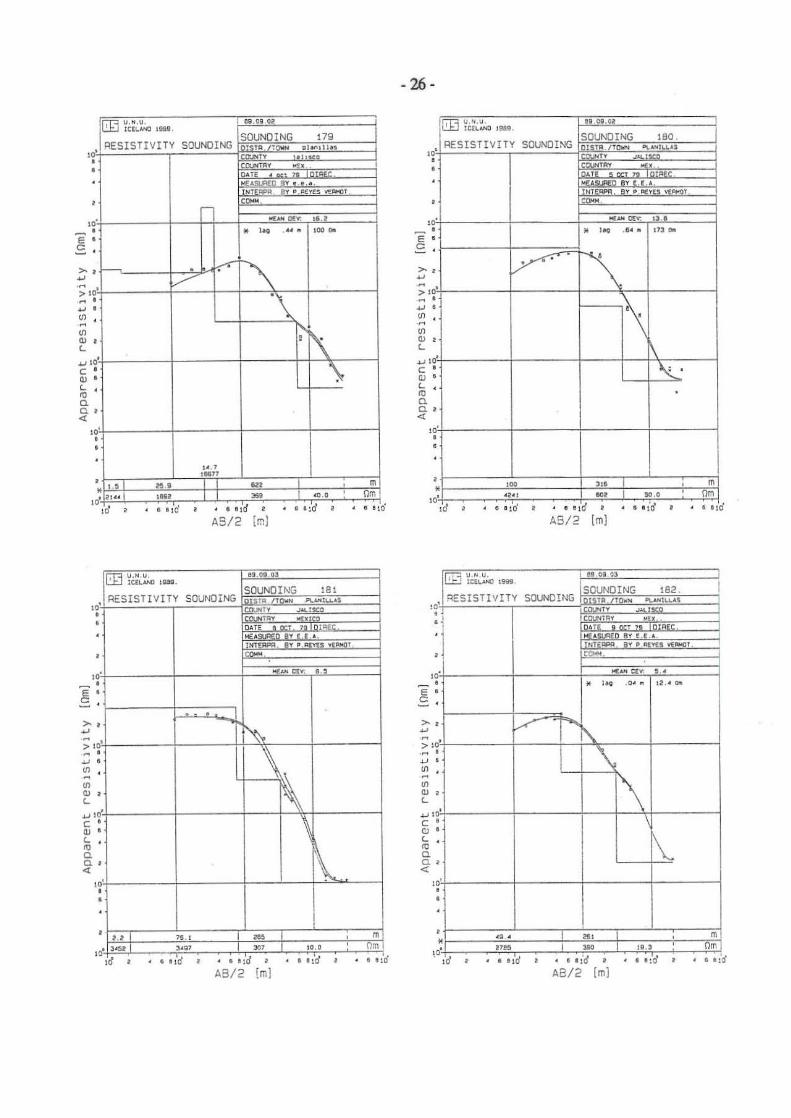
- 26-

RESISTIVITY

E , '" ," . ,~" , '" .s ... " e

oS oS ~ ~ ~ ~

>'

~ ~

0 0

" 0 ~

• • C C

~, ~

C C

• • C C

• • "- "-"- "-

" '"

. . .. . . . . . . A8/2 10] AS/2 [mJ

RESISTIVITY SOUNDiNG RESISTIVITY SOUNDING

~ • '" .0< .. !I, o "" , e c

~ ~,

~ ~

> > " ~ ~

0 0

0 • C

~

C • c ro Q a '"

. . , . . . . . , . . AB/2 [mJ A8/2 [mJ

- Z7-

,-!;ESIST

• • 0= c

> > ~ ~

> ~ ~

• • " • • L

C • L m

" " ~

. . . . . . . .. AB/2 (m)

,-IVITY SOUNDING RESISTIVITY

• ~ c

> > ~ ~

> " ." ~ ~ • • • • • • L L

~

C • L m " " ~

.. . . . . • • AB/2 iml A8/2 ImJ

- 28-

, ~,

~ESIST I vrTY SOUNDING SOUNDING

E E C C

> > ~ ~

" >. ~

~ • • • • • L • L ~,

~ C • C L • "

L 0. 0 0. n ., n .,

. . . . . . AB/2 [mJ

' .. ~ESIST I V I TY SOUNOING SOUNDING

E E c c

> > ~ ~

" > " ~ ~

• • • • W • C L

~ . ~

C C • W L L

" " 0. 0. 0. 0. ., .,

• • . . A3/2 ImJ AB/2 [m]

- 29-

RESIST IVI TY SOUNDING SOUNDI NG

, . , . AB/2 [mJ A8/2 Iml

" " c c

~ ~

~ ~

> >

~ ~

• • " • • • • L L

~ ~

c c • • L L m m

" " " " ~ ~

, . , . , . , .. '8/2 Iml Aa/2 (mJ

- 30-

- 31 -

APPENDIX ID

Two dimensional interpretation of Schlumberger soundings_

FELIX-program:

Measured apparent resIStIVIty curves (shown as points) and calculated apparent resistivity curves (shown as continuous curves). The two dimensional model is shown in figure 12 in the main report.

- 32-

·33·

~ESIST IVITY SOUNDING SOUNDING

E E C E > > ~ ~

. ; \ ' . • > " ~ ~

" " ." " " • • L L

~

C • L ro n n ~

• • ' I • " 1 . . .. • 6. ! .. " .. AB/2 [m ] AB/2 [m l

RESISTIVITY SOUNDING SOUNDING

.. . E

.. • E .. ' • c c . > . . > ~ ~

." " >' >'

~ ~

" " " " • • L L

~

C C

• • L L ro ro a a n n ~ ~

.. . . . . . ·'1 . . • • 11

A8/2 Iml A8/2 Iml

E EO

RESIST[VITY

•• .., J

>'!T------~----+-~~~------

~'!T------_f------_f------_f~------c • L ro n n .,

.. • • 11 .. AB / 2 [ml

.. .

~,4-----+----~--~--~ c • L ro n n ., '!~----+------~---~---~

. . . . .. •• AB/2 [ml

·34·

• • ! •

.. . . . . . . A8/2 Iml

RESISTIVITY SOUNDING

~'!~-----+------~---~---~ c • L ro n n .,

. . . . A8/2 Iml

.. . .

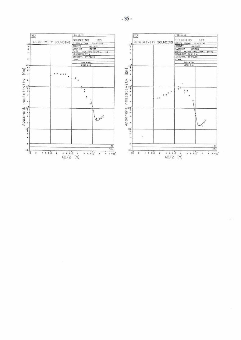
- 35 -

~ESISTrVITY SOUNDING

E E

'" .. . .. C

> > ~ ~

~ ~

m m m m • • L L

~

C • L ro

" " ~

. . .. . . . . AB/2 [mJ AB/2 Im l