reservoir modelling wabamun area co sequestration … simulations.pdf · 2010-02-02 · energy and...
TRANSCRIPT

Energy and Environmental Systems Group
Institute for Sustainable Energy, Environment and Economy (ISEEE)
Reservoir Modelling
Wabamun Area CO2 Sequestration Project (WASP)
Authors Seyyed Ghaderi
Yuri Leonenko
Rev. Date Description Prepared by
1 August 14, 2009 First draft Yuri Seyyed
2 August 19, 2009 Revision Yuri Seyyed

Wabamun Area CO2 Sequestration Project (WASP) Page 2 of 27
Reservoir Modelling
Table of Contents
INTRODUCTION ........................................................................................................................................... 5
DISCUSSION ................................................................................................................................................ 5
1. NUMERICAL RESERVOIR MODELLING .............................................................................................. 5 1.1. Preliminary Conceptual Model ......................................................................................................... 5 1.2. Detailed Model with Full Aquifer (Nisku) Extent ............................................................................... 9
2. LONG-TERM FATE OF CO2 ................................................................................................................ 17 2.1. Pressure Field Evolution During and After Injection Until Initial Reservoir Pressure Reached ..... 17 2.2. Effect of Aquifer Dip on Plume Movement and Size ...................................................................... 18 2.3. Estimation of Timescale for Free-Phase CO2 after Injection (onset and dissolution time for
natural convection scenario) .......................................................................................................... 18
3. INVESTIGATION OF THE PHASE BEHAVIOR OF H2S SATURATED BRINE IN CO2 SEQUESTRATION PROCESS ............................................................................................................ 19 3.1. Fluid Representation of CO2-Brine and CO2-H2S-Brine Systems .................................................. 19 3.2. Description of the Simulation Model .............................................................................................. 20 3.3. General Simulation Results ........................................................................................................... 20 3.4. Base Case Simulation Results and Observations ......................................................................... 22 3.5. Sensitivity Analysis ......................................................................................................................... 23
SUMMARY .................................................................................................................................................. 26
ACKNOWLEDGMENTS .............................................................................................................................. 26
REFERENCES ............................................................................................................................................ 27

Wabamun Area CO2 Sequestration Project (WASP) Page 3 of 27
Reservoir Modelling
List of Tables
Table 1: Reservoir properties. ....................................................................................................................... 6

Wabamun Area CO2 Sequestration Project (WASP) Page 4 of 27
Reservoir Modelling
List of Figures
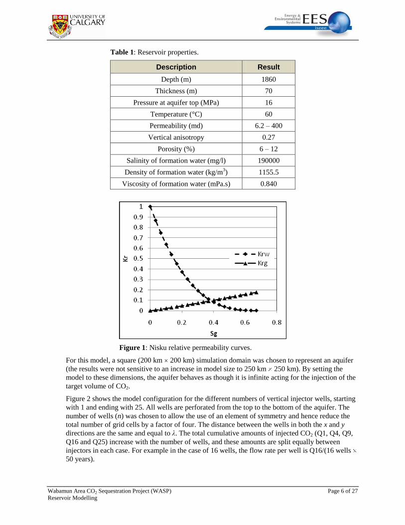
Figure 1: Nisku relative permeability curves. ................................................................................................ 6
Figure 2: Configuration of injection wells and element of symmetry (salmon area). .................................... 7
Figure 3: Effect of different parameters on storage capacity: a) effect of distance between wells, b) effect of compressibility, c) effect of permeability, d) effect of aquifer thickness. ..................................... 8
Figure 4: Top view of the Nisku formation in the Wabamun Lake area (left), study area is outlined in red and base formation/properties used are shown on the right. ............................................................... 10
Figure 5: Plume extension (top row) and pressure radius of investigation (bottom row) after 50 years of injection for different wells in the Nisku study area (within the red area in Figure 4) ............... 10
Figure 6: Pressure evolution: left, one well; right, 10 wells. ........................................................................ 11
Figure 7: Variation of Nisku capacity with respect to number of wells and formation properties (red curve represents base properties). ............................................................................................................. 12
Figure 8: Pressure at the end of injection. .................................................................................................. 12
Figure 9: Comparison of the effect of different well orientations and stimulation on the storage capacity of the model. ................................................................................................................................. 13
Figure 10: Five geo-statistical realizations for porosity and permeability. .................................................. 14
Figure 11: Object-based realization of porosity. ......................................................................................... 14
Figure 12: Saturation (left) and pressure (right) fields for stochastic modelling after 50 years of injection. ...................................................................................................................................................... 15
Figure 13: Injection capacity for five realizations. ....................................................................................... 15
Figure 14: Injection capacity for different fracture pressures. ..................................................................... 15
Figure 15: Saturation (left) and pressure (right) fields for object-based modelling after 50 years of injection. ...................................................................................................................................................... 16
Figure 16: Injection capacity for object-based modelling. ........................................................................... 16
Figure 17: Pressure evolution (each well injects 0.5 Mt/year for 50 years). ............................................... 17
Figure 19: Saturation field for a single injector: a) base properties; b) permeability is increased to 150 mD. ....................................................................................................................................................... 18
Figure 20: Short-term (a) and long-term (b) processes involved in geological storage. ............................ 19
Figure 21: Water-gas relative permeability curves. .................................................................................... 20
Figure 22: Variation of gas saturation around the injection well after 200 days. ........................................ 21

Wabamun Area CO2 Sequestration Project (WASP) Page 5 of 27
Reservoir Modelling
INTRODUCTION
Although it is recognized that deep aquifers offer the potential for very large storage capacities for
CO2 sequestration, it is not clear what the best method is to fill these aquifers with large volumes of
CO2 in a relatively short period of time within localized injection areas. The typical benchmark for
the rate of CO2 injection is 1 Mt/year when studying storage performance. This rate is very low
when compared to the scale needed for storage technology to play a significant role in managing
global emissions. In this report we study the feasibility of injecting large volumes of CO2 into the
Nisku aquifer, which is located in the Wabamun Lake area in Alberta, Canada [1]. In this area,
large CO2 emitters include four coal-fired power plants with emissions that range between 3 and
6 Mt/year each, which together emit ~ 20 Mt/y or ~ 1 Gt over 50 years. This number, 1 Gt, is
considered the target capacity for WASP. The Nisku aquifer is believed to be a suitable choice for
future sequestration projects. The main objectives of the WASP study are as follows.
i) Estimate storage capacity. Traditionally, storage capacity is determined by available pore
space. For this study a more practical aspect was used—the maximum amount that can be
injected within a short period of time ( ~ 50 years) within a localized injection area (~ 30
km × 90 km). The capacity of individual reservoirs to accommodate large injection
volumes should be evaluated by assessing the ability to inject CO2 without exceeding
formation fracture pressures. A number of options were also considered to increase storage
capacity.
ii) Determine CO2 plume movement and pressure distribution. These factors were determined
for the period during and after injection. The shape and dip of the aquifer, the number of
wells and their placement (among other parameters) would be considered.
iii) Estimate long-term fate of injected CO2. Estimate the timescale for the long-term fate of the
injected CO2 associated with free-phase CO2, aquifer pressurization, and the effect of dip
on plume shape and its migration.
iv) Investigate phase behaviour. Investigate the phase behaviour of H2S initially saturated in
brine in the CO2 sequestration process.
DISCUSSION
1. NUMERICAL RESERVOIR MODELLING
1.1. Preliminary Conceptual Model
To develop a benchmark at the beginning of the project, a simplified conceptual model was
developed based on homogeneous properties and an infinite acting aquifer. The properties for the
simulations were taken from Hitchon, 1996 [1] (Table 1). The table data was then revised using
WASP preliminary analysis data: permeability was changed to 30 md, porosity to 10%, aquifer
thickness to 70 m and PVT table for density and viscosity were generated based on Hassanzadek et
al, 2008 [2]. The relative permeability curves (Figure 1) were taken from literature (Bennion and
Bachu, 2005 [3]).
Wabamun Area CO2 Sequestration Project (WASP) Page 6 of 27
Reservoir Modelling
Table 1: Reservoir properties.
Description Result
Depth (m) 1860
Thickness (m) 70
Pressure at aquifer top (MPa) 16
Temperature (°C) 60
Permeability (md) 6.2 – 400
Vertical anisotropy 0.27
Porosity (%) 6 – 12
Salinity of formation water (mg/l) 190000
Density of formation water (kg/m3) 1155.5
Viscosity of formation water (mPa.s) 0.840
Figure 1: Nisku relative permeability curves.
For this model, a square (200 km 200 km) simulation domain was chosen to represent an aquifer
(the results were not sensitive to an increase in model size to 250 km 250 km). By setting the
model to these dimensions, the aquifer behaves as though it is infinite acting for the injection of the
target volume of CO2.
Figure 2 shows the model configuration for the different numbers of vertical injector wells, starting
with 1 and ending with 25. All wells are perforated from the top to the bottom of the aquifer. The
number of wells (n) was chosen to allow the use of an element of symmetry and hence reduce the
total number of grid cells by a factor of four. The distance between the wells in both the x and y
directions are the same and equal to λ. The total cumulative amounts of injected CO2 (Q1, Q4, Q9,
Q16 and Q25) increase with the number of wells, and these amounts are split equally between
injectors in each case. For example in the case of 16 wells, the flow rate per well is Q16/(16 wells
50 years).

Wabamun Area CO2 Sequestration Project (WASP) Page 7 of 27
Reservoir Modelling
Figure 2: Configuration of injection wells and element of symmetry (salmon area).
Single Injector (capacity and plume size)
The saturation and pressure fields for a single well, as well as for multiple injection scenarios, will
be shown in the following section (Section 1.2, Detailed Model with Full Aquifer Extent), since the
results are very similar. A brief summary for a single injector:
plume radius after 100 years of simulation is ~ 4.6 km; and
capacity of one vertical well is ~ 1 Mt/y (based on Pf = 40 MPa), horizontal well improves
capacity with a maximum rate of ~ 1.5 Mt/y. (The value for the fracture pressure will be
discussed later in this report.)
Multiple Injectors
For multiple (n>1) injection scenarios, CO2 saturation plumes have no interference and n individual
plumes have a radius of 4 to 5 km for each injector.
The pressure field behaves totally different than the saturation field. By the fiftieth (50th) year of
CO2 injection, there are no individual pressure plumes. Instead, most of the pressure plumes have
merged into a single large (scale of hundred km) pressure disturbance. Injection capacity increases
with the number of wells, but there is limited benefit to adding incremental wells after 15 to 20.
These phenomena will be discussed in detail in Section 1.2 when more advanced modelling for the
Nisku aquifer is considered.
Sensitivity of Injectivity to Different Reservoir Properties (permeability, rock compressibility, aquifer depth) and Well Placement (generic study)
The sensitivity study in this section was performed using generic variables. The properties of the
reservoir were chosen similarly to those used in the Berkeley Laboratory inter-comparison study
[4]. This study and its properties are well known, so they could be used as a benchmark for
representative aquifers for generic studies. The aquifer is considered to be homogenous, isotropic,
and isothermal with a thickness of 100 m and permeability of 1.0 × 10⁻¹³
m2 (100 mD), porosity is
12%, rock compressibility of 4.5 × 10⁻¹⁰
1/Pa, and fracture pressure equal to 30,000 kPa. In all runs,
the initial conditions include a temperature of 45°C, pressure of 12000 kPa, salinity of 15% of NaCl
by weight, brine saturation of 1, and gas saturation of zero. All simulation runs involve continuous
injection for 50 years. Bottom hole injection pressure is monitored and constrained to less than
27 MPa over the entire injection period. These parameters define a maximum CO2 storage capacity
over a period of 50 years.
Figure 3-a shows the storage capacity considering the number of vertical wells and the distance
between them. As this figure indicates, the required number of wells to achieve the target volume
(1 Gt of total injection) is 25 situated 8 km apart. For practical reasons it may be better to use a
smaller or larger number of wells covering a larger or smaller area. Extrapolating the green and red
curves, we can roughly estimate the number of wells required. For example, 18 wells that are 10 km
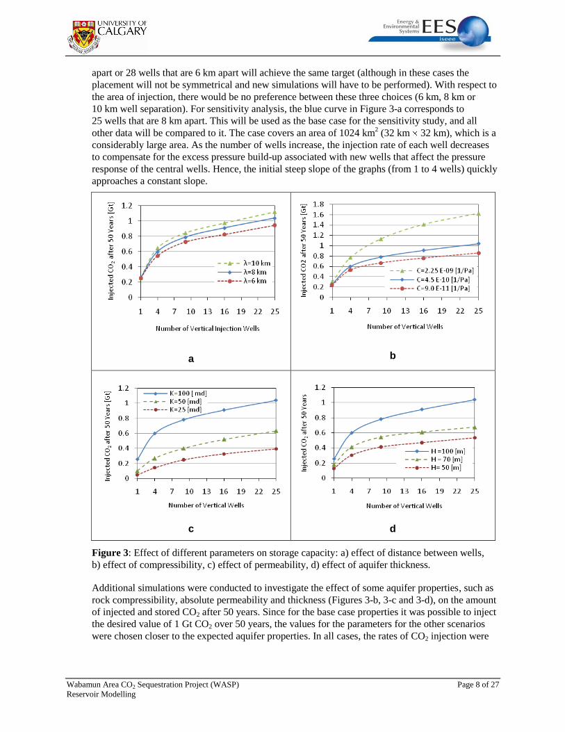
Wabamun Area CO2 Sequestration Project (WASP) Page 8 of 27
Reservoir Modelling
apart or 28 wells that are 6 km apart will achieve the same target (although in these cases the
placement will not be symmetrical and new simulations will have to be performed). With respect to
the area of injection, there would be no preference between these three choices (6 km, 8 km or
10 km well separation). For sensitivity analysis, the blue curve in Figure 3-a corresponds to
25 wells that are 8 km apart. This will be used as the base case for the sensitivity study, and all
other data will be compared to it. The case covers an area of 1024 km2 (32 km 32 km), which is a
considerably large area. As the number of wells increase, the injection rate of each well decreases
to compensate for the excess pressure build-up associated with new wells that affect the pressure
response of the central wells. Hence, the initial steep slope of the graphs (from 1 to 4 wells) quickly
approaches a constant slope.
a
b
c
d
Figure 3: Effect of different parameters on storage capacity: a) effect of distance between wells,
b) effect of compressibility, c) effect of permeability, d) effect of aquifer thickness.
Additional simulations were conducted to investigate the effect of some aquifer properties, such as
rock compressibility, absolute permeability and thickness (Figures 3-b, 3-c and 3-d), on the amount
of injected and stored CO2 after 50 years. Since for the base case properties it was possible to inject
the desired value of 1 Gt CO2 over 50 years, the values for the parameters for the other scenarios
were chosen closer to the expected aquifer properties. In all cases, the rates of CO2 injection were

Wabamun Area CO2 Sequestration Project (WASP) Page 9 of 27
Reservoir Modelling
adjusted such that at the end of injection period, the maximum bottom-hole pressure reached the
highest sustainable pressure.
Depending on the rock composition of the formations, the compressibility of the reservoirs varies
widely. Hence for sensitivity study, the value of compressibility was varied within one order of
magnitude by multiplying and dividing the base case value by five, respectively. Figure 3-b shows
the outcome. Higher values of compressibility cause significant differences on the results,
especially when the number of well increases.
The permeability of the formation controls both the pressure distribution over the system volume
and the propagation velocity of the pressure pulse away from the injection site. According to the
diffusivity equation, pressure will diffuse faster in formations with higher permeability or lower
compressibility. Although it is quite possible to find localized regions with high absolute
permeability within an aquifer (which are usually allocated to injection sites), generally the average
permeability of the formation may be low. Figure 3-c depicts the results of simulations for different
values of permeability. As the permeability is reduced by half, the amount of stored CO2 nearly
decreases by half. By reducing the permeability, the initial steep slope of the previous curves
decreases. This illustrates that increasing the number of wells does not contribute significantly to
capacity in low permeable formations.
The last parameter considered was the thickness of the formation. Reducing the thickness by 50%
of the initial value has almost the same effect as reducing the absolute permeability by half (as
would be anticipated). Figure 3-d indicates that for thinner reservoirs, more wells should be placed
in the injection zone or other methods for increasing injectivity should be considered.
1.2. Detailed Model with Full Aquifer (Nisku) Extent
In the following section, the simulation results for CO2 injection in the Nisku formation will be
presented. First, a homogenous model is used to investigate the performance of a semi-infinite
formation on injectivity. Then a heterogeneous model is populated with realistic permeability and
porosity fields in order to demonstrate the effect of heterogeneity and reservoir dip angle on the
evolution of a CO2 plume and the associated impact on reservoir pressure.
Development of Full Aquifer Extent Geometry
Figure 4 shows the top view of the Nisku aquifer. The region covers an area of about 450 km ×
640 km, while the bounded area by the red line shows the focus injection area. The majority of core
and log data are related to available wells in this area and the injection site will be confined within
this boundary. The area of this focus region is approximately 1500 km2. The thickness of the
numerical model is 70 m. Thirty layers with variable thickness are used to create the 3D model. The
base properties used are the same as for the conceptual model.

Wabamun Area CO2 Sequestration Project (WASP) Page 10 of 27
Reservoir Modelling
Properties Used as a Base
Depth 1860 m
Thickness 70 m
Temperature 60oC
Permeability 30 mD
Porosity 10%
Salinity 190,000 mg/l
Rock
Compressibility
4.5 10-7
1/KPa
Figure 4: Top view of the Nisku formation in the Wabamun Lake area (left), study area is outlined
in red and base formation/properties used are shown on the right.
Plume Size and Pressure Field Depending on Number of Injectors
Figure 5 presents the plume extension and pressure distribution after 50 years of injection using the
base case properties. For the case with one well, the plume radius at the top layer is about 4.6 km,
which is consistent with the conceptual model as well as the analytical solution radius [5]. It is
noticeable that the size of the ―pressure plume‖ is much larger at about 65 km, even for one well. In
the cases of n number of injectors, one can see n individual plumes for CO2 saturation. As the
number of wells increase, the individual injector flow rate decreases (fracture pressure constraint)
and consequently the plume radius decreases. However for pressure, one can see a very strong
interference between injectors that pressurizes the total area of injection. The pressure build-ups
and soon merges, and thereafter a cumulative pressure disturbance dissipates radially away from a
central position, which is the well position for one well model and is near the centre of the focus
area for the models.
Figure 5: Plume extension (top row) and pressure radius of investigation (bottom row) after
50 years of injection for different wells in the Nisku study area (within the red area in Figure 4)

Wabamun Area CO2 Sequestration Project (WASP) Page 11 of 27
Reservoir Modelling
It is very important to mention that the dynamics of the pressure field is very different for one
injection well, Figure 6 left, than for multiple injection wells, Figure 6 right.
Figure 6: Pressure evolution: left, one well; right, 10 wells.
One can see that the pressure fall-off after ending CO2 injection is much quicker for a single well.
The pressure fall-off for multiple wells is delayed because of the larger pressure influence area.
Injection Capacity (versus number of wells and its sensitivity to different properties)
Starting with one well, the maximum achievable rate was determined to be as high as 1.1 Mt
CO2/year (matching the results of the conceptual model), which is equivalent to 0.055 Gt after
50 years. This flow rate causes the bottomhole pressure to reach 40 MPa at the end of the injection
period. This value was assumed by the WASP team at the beginning of the project based on some
literature data for Alberta reservoirs. Midway through the project, the Geomechanical Simulation
Group estimated this value to be around 35 to 37 MPa. Since our original assumption was very
close to the new calculated value (which is not based on real field data), we decided to keep
40 MPa in our reservoir model. The sensitivity of capacity to different fracture pressure (within the
range 30 to 40 MPa) is presented later in this section. Also there is discussion (in the
Geomechanical Simulation Group Report) of the impact of pressure difference on fracture pressure
during injection.
When the next five wells are placed in the zone, the corresponding flow rate for each well is
reduced to 0.625 Mt/year per well with cumulative injection of 0.15 Gt. Increasing the number of
wells to 10 brings the flow rate to 0.418 Mt/year per well with total injected CO2 of 0.209 Gt.
Finally, the values for 20 wells are equal to 0.238 Mt/year and 0.238 Gt, respectively. These results
are shown in Figure 7, red curve. We also determined what reservoir properties we would need to
achieve the target of 1 Gt. The green curve on Figure 7 presents the injection capacity of the focus
area with the following aquifer properties: porosity 20% and horizontal permeability 90.0 (mD).
Although these values caused a significant difference in the outcome, the limitation in injectivity
improvement for more than 10 wells still existed. It could not be claimed that these values are the
maximum injectivity and storage of the formation because no optimization with respect to well
positioning and flow rate was performed.

Wabamun Area CO2 Sequestration Project (WASP) Page 12 of 27
Reservoir Modelling
Figure 7: Variation of Nisku capacity with respect to number of wells and formation properties
(red curve represents base properties).
Some Options to Increase Capacity (horizontal injection, fracturing)
In the storage process the term ―capacity‖ could have two meanings. The apparent capacity is the
available and accessible pore volume of the aquifer, and the injection capacity is the amount of CO2
that can be realistically injected into the formation and is a function of the number of wells and the
fracture pressure of the formation and the confining caprock [6]. As discussed earlier, for a
restricted injection area such as in the Nisku study, increasing the number wells beyond a certain
limit (which is controlled by formation properties and injection site area) has a minor effect on the
injection capacity. The focus of this section is to investigate methods that lead to an increase in
injection capacity in the aquifer.
The first method is to use horizontal wells instead of vertical wells. For vertical wells, it is
preferable to use fully penetrated wells over the entire thickness of the aquifer. To find the
minimum length for a horizontal well, the effective radius of pressure disturbance around the
vertical injection well, which is again a function of formation properties, should be determined. For
vertical wells, as the injection begins the pressure around the wellbore increases rapidly and causes
the development of locally narrow width pressure peaks in the vicinity of the well, Figure 8.
Figure 8: Pressure at the end of injection.

Wabamun Area CO2 Sequestration Project (WASP) Page 13 of 27
Reservoir Modelling
Using horizontal wells with total length greater than the scale of the vertical injection well’s
pressure peak ―L” (for the Nisku formation this minimum required well was estimated to be equal
to 3000 m) will diminish these peaks and increase injectivity, Figure 9 (H-Well Bar). The V-Well
Bar corresponds to vertical injectors.
*HF: Hydraulic Fracture
Figure 9: Comparison of the effect of different well orientations
and stimulation on the storage capacity of the model.
The application of stimulation techniques, such as hydraulic fracturing, can improve injectivity as
long as the caprock is not fractured. The technical feasibility of implementing these techniques
requires careful geomechanical characterization of the formation. Vertical wells with hydraulic
fractures were modelled by constructing thin grid blocks 400 m (fracture half length) from the well
grid toward the east and west. A porosity of 0.15 and permeability of 1500 mD were assigned to
these grid blocks to approximate a 400 m half-length fracture and associated damage zone. These
properties were also used to construct four 100 m half lengths of four staggered hydraulic fractures
for the horizontal wells. The V-Well (HF) and H-Well (HF) bars in Figure 9 shows the simulation
results for 10-wells cases (located as in Figure 8) in the Nisku aquifer (V = vertical wells, H =
horizontal). Another promising method of increasing CO2 capacity would be to produce the brine
[7] from the formation to prevent the reservoir pressure from building up excessively near the
injection wells. This method involves transporting produced brine through surface pipelines to a
location where the brine can be injected into another compatible formation or into a lower pressure
region of the Nisku aquifer itself.
Heterogeneity Sensitivity Study
Two kinds of heterogeneity were considered in this study: stochastic and object-based models.
The stochastic model was based on existing quantitative data (i.e., wireline log, acoustic
impedance) and geostatistical tools. It relies on resistivity-derived porosities and permeabilities
from nearly 60 wells. For this study, five equiprobable realizations of properties (porosity, %: max-
28.6, min-1.3, mean-4.9) and (permeability, mD: min-3.1; max-393; mean-22.37) were generated,
see Figure 10. All sets of realizations for this section (heterogeneity sensitivity study) were
developed by the geostatistics group and the detailed description of these realizations and the
methodology is presented in the Geomodelling Section of this report, which was written by Chris
Eisinger and Jerry Jensen.

Wabamun Area CO2 Sequestration Project (WASP) Page 14 of 27
Reservoir Modelling
Figure 10: Five geo-statistical realizations for porosity and permeability.
Object-based models define ―objects‖ (same sizes) as higher porosity and permeability zones, the
geometry and distribution which are constrained by dimensions of existing modern carbonate
analogs, conceptual understanding of Nisku carbonate in the Wabamun area, wireline log data and
seismic data.
Two kinds of objects: i) dark blue (Minor width-500 m, Major/Minor ratio -5 and Thickness -5 m)
and ii) light blue (Minor width-300 m, Major/Minor ratio -5 and Thickness -2 m) all oriented along
the dip were distributed in each zone (upper, middle, and lower, see Figure 11 left) of the Nisku
open marine. Figure 11 right (Upper third has 13 layers with average vertical grid size z = 1.72 m;
Middle third has 5 layers with z = 4.46 m and Lower third has 12 layers with average z = 1.86 m).
Figure 11: Object-based realization of porosity.

Wabamun Area CO2 Sequestration Project (WASP) Page 15 of 27
Reservoir Modelling
For the stochastic modelling examples (realizations 4 and 5), the saturation and pressure fields are
shown in Figure 12.
Figure 12: Saturation (left) and pressure (right) fields for stochastic modelling after 50 years of
injection.
Although one can see some differences on a small scale for both fields, the injection capacities for
all cases are almost identical (Figure 13), and very close to being homogeneous (Figure 7 for
10-well injection).
Figure 13: Injection capacity for five realizations.
The above results represent the storage capacity when the fracture pressure was set to 40 MPa.
Sensitivity of capacity to fracture pressure is shown in Figure 14.
Figure 14: Injection capacity for different fracture pressures.

Wabamun Area CO2 Sequestration Project (WASP) Page 16 of 27
Reservoir Modelling
For object-based modelling, the saturation and pressure fields are shown in Figure 15.
Figure 15: Saturation (left) and pressure (right) fields
for object-based modelling after 50 years of injection.
Injection capacity, as in the case of stochastic modelling, is very close to the homogeneous model,
see Figure 16.
Figure 16: Injection capacity for object-based modelling.
Based on this limited number of realizations, it is possible to suggest that the small (compared to
plume size) scale heterogeneity considered in this study does not play a strong role for pressure and
saturation fields and for overall capacity of the injection site. For layered systems and for objects
comparable to plume size it will be significant, especially by selective placement of injectors. Such
a study would require more detailed knowledge of the distribution properties within the aquifer.

Wabamun Area CO2 Sequestration Project (WASP) Page 17 of 27
Reservoir Modelling
2. LONG-TERM FATE OF CO2
In this section, we discuss the long-term fate associated with the following phenomenon:
Increased aquifer pressure during and after injection.
Migration of CO2 beyond injection area due to dip.
Buoyant phase of CO2 over long periods of time.
2.1. Pressure Field Evolution During and After Injection Until Initial Reservoir Pressure Reached
As discussed in previous sections, the pressure in the aquifer (within and around the injection area)
will increase during the injection period and then gradually decrease to the initial pressure
distribution, due to the very large volume in the Nisku aquifer. It is important to know how long it
will take for a substantial pressure disturbance to dissipate. The simulation results of a 10-well
scenario are presented in Figure 17.
Figure 17: Pressure evolution (each well injects 0.5 Mt/year for 50 years).
One can see that the pressure does not reach initial reservoir pressure (Pi = 16 MPa) even 650 years
after injection stops, although the difference in P is small compared to the maximum difference
( Pmax=24 MPa = Pf-Pi at the end of injection). The graph of P versus time is presented in
Figure 18, which allows for estimating the timescale of pressure decay.
0
5
10
15
20
25
30
0 200 400 600 800
Years
MP
a
Figure 18: P versus time.

Wabamun Area CO2 Sequestration Project (WASP) Page 18 of 27
Reservoir Modelling
From this graph (assuming exponential behavior), P falls e ( ~ 2.7) times at ~ 120 years, thereby
providing the timescale of high pressure fate for injection design.
2.2. Effect of Aquifer Dip on Plume Movement and Size
The effect of aquifer dip was evaluated by simulations using the base Nisku properties (Figure 4)
for single-well injection at a rate of 1 Mt/year for 50 years. Simulations run up to 1000 years after
injection started and two cases were considered for comparison: i) dip = 0 and ii) dip = 0.5o. The
results of CO2 saturation at the top layer versus time are shown in Figure 19. One can see that at
base conditions the effect of dip on the plume movement is marginal (Figure 19-a), although when
permeability was increased (while all other parameters remained the same) noticeable plume
migration along the dip was observed (Figure 19-b).
a)
b)
Figure 19: Saturation field for a single injector: a) base properties; b) permeability is increased to
150 mD.
What this means is if the plume reaches regions with higher permeability, it will migrate upwards
and this should be taken into consideration.
2.3. Estimation of Timescale for Free-Phase CO2 after Injection (onset and dissolution time for natural convection scenario)
The CO2 injected into a deep aquifer is typically 10 to 40% less dense than the resident brine.
Driven by density contrasts, CO2 will first flow vertically and then horizontally spread under the
caprock. If there are breaches in the caprock, leakage could occur through these high permeability
zones or through artificial penetrations, such as abandoned wells. It is very important to know how
long free-phase CO2 remains in the reservoir and how long complete dissolution of CO2 into the
brine takes because this determines the time that free-phase CO2 has to leak from the formation.
After injection, free-phase CO2 (gas or supercritical fluid) will be partially trapped as residual
saturation and the remainder will slowly dissolve in the brine [8]. Depending on reservoir
properties, different mechanisms may be responsible for dissolution. In this section we estimated
the dissolution mechanisms for the Nisku conditions and associated timescale of dissolution. The
analysis is based on Hassanzadeh et al, 2007 [9]. In the short term (Figure 20 a), during and after
injection, some amount of CO2 is residually trapped and the remainder may be dissolved by natural
convection (Figure 20 b). First, we found convective mechanisms in the Nisku aquifer or at Nisku
conditions, then we estimated the onset of natural convection and the corresponding timescale.

Wabamun Area CO2 Sequestration Project (WASP) Page 19 of 27
Reservoir Modelling
a) b)
Figure 20: Short-term (a) and long-term (b) processes involved in geological storage.
The important parameter to describe the stability of such a system is the porous medium Rayleigh
number. It is defined by
where
k is permeability,
is porosity,
g is acceleration due to gravity,
H is aquifer thickness,
is viscosity,
is the density difference (CO2 saturated and fresh brine), and
D is the molecular diffusion coefficient.
If Ra > 49 — natural convection occurs, Hassanzadeh et al, 2007 [9]. For the Nisku conditions, Ra
is ~ 400 from which we estimated the onset of convection at these conditions (tonset ~ 80 years) and
timescale of convective dissolution (Tdis ~ 3000 years). Estimations are made based on Hassanzadeh
et al, 2007 [9].
3. INVESTIGATION OF THE PHASE BEHAVIOR OF H2S SATURATED BRINE IN CO2 SEQUESTRATION PROCESS
It was found (see the Geochemistry section of this report) that the Nisku brine includes dissolved
H2S. The folloing section investigates the behavior of H2S during the CO2 sequestration process.
3.1. Fluid Representation of CO2-Brine and CO2-H2S-Brine Systems
The solubility of gaseous components in the aqueous phase in CMG-GEM [10] is modelled by
employing Henry’s law. The fugacity of components is calculated using the Peng-Robinson
Equation-of-State. GEM version 2008.12 uses accurate models for the Henry’s constants of CO2
and H2S taking into account pressure, temperature and salinity (salting-out coefficient) by Harvey
semi-empirical correlation [11]. At initial condition of the Nisku formation (pressure = 16 MPa,
temperature = 60°C, and salinity = 190,000 mg/litre), the CMG calculates the concentration of
dissolved H2S in a saturated brine equal to 0.023 by mole fraction in the aqueous phase, which
D
HkgRa
Wabamun Area CO2 Sequestration Project (WASP) Page 20 of 27
Reservoir Modelling
aligns with the value reported in the literature, Duan et al, 2007 [12]. For calculating the viscosity
and density of the aqueous phase, Kestin’s [13] and Rowe’s [14] correlation were used
respectively.
3.2. Description of the Simulation Model
Since the focus of this study was to investigate the fate of existing H2S in the Nisku formation
during CO2 injection, the simulation was limited to a single well located at the centre of a bounded
radial model with a production well at the boundary to mimic a constant pressure boundary
condition. Therefore, simulations were performed in a one-dimensional radial (r x z = 1) model
with the total extend: radius of 500 m and a net aquifer thickness of 5 m. The absolute permeability
and porosity of the model were equal to 2000 md and 0.3, respectively to allow proper propagation
of CO2 plume after a few days. With respect to initial concentration of dissolved H2S, two cases
were considered. In the first case the initial mole fraction of dissolved H2S was taken as 0.02; and
in the second case as 0.005 (the balance being water).
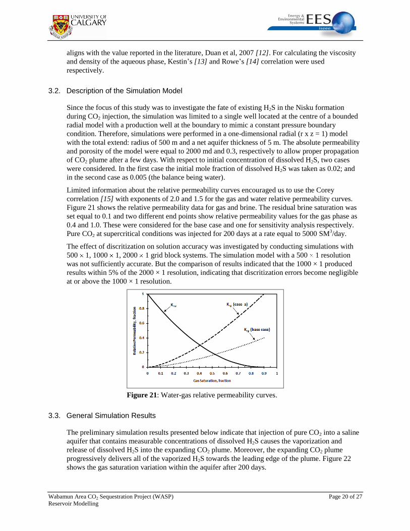
Limited information about the relative permeability curves encouraged us to use the Corey
correlation [15] with exponents of 2.0 and 1.5 for the gas and water relative permeability curves.
Figure 21 shows the relative permeability data for gas and brine. The residual brine saturation was
set equal to 0.1 and two different end points show relative permeability values for the gas phase as
0.4 and 1.0. These were considered for the base case and one for sensitivity analysis respectively.
Pure CO2 at supercritical conditions was injected for 200 days at a rate equal to 5000 SM3/day.
The effect of discritization on solution accuracy was investigated by conducting simulations with
500 1, 1000 1, 2000 1 grid block systems. The simulation model with a 500 1 resolution
was not sufficiently accurate. But the comparison of results indicated that the 1000 × 1 produced
results within 5% of the 2000 × 1 resolution, indicating that discritization errors become negligible
at or above the 1000 × 1 resolution.
Figure 21: Water-gas relative permeability curves.
3.3. General Simulation Results
The preliminary simulation results presented below indicate that injection of pure CO2 into a saline
aquifer that contains measurable concentrations of dissolved H2S causes the vaporization and
release of dissolved H2S into the expanding CO2 plume. Moreover, the expanding CO2 plume
progressively delivers all of the vaporized H2S towards the leading edge of the plume. Figure 22
shows the gas saturation variation within the aquifer after 200 days.

Wabamun Area CO2 Sequestration Project (WASP) Page 21 of 27
Reservoir Modelling
Figure 22: Variation of gas saturation around the injection well after 200 days.
As shown in Figure 23, the mole fraction of CO2 within this plume changes from 1.0 at the point of
injection and gradually decreases toward zero close to the outer boundary of the plume.
Figure 23: Variation of CO2 mole fraction ( vCO2
y ) in the gas phase after 200 days of CO2 injection.
Note that the mole fraction of H2S ( vH2
y S ) at any location is equal to vCO2
y1.0 .

Wabamun Area CO2 Sequestration Project (WASP) Page 22 of 27
Reservoir Modelling
Figure 24 illustrates the variation in the composition of the plume after 200 days as a side view.
Figure 24: Side view of the variation of CO2 mole fraction in the gas phase after 200 days. This
figure also shows the position of the production well.
Since the plume expansion is symmetrical in the radial models, it is reasonable to use 2D graphs to
better illustrate the development of gas saturation and H2S evolution as the vaporizing gas drive
progresses.
3.4. Base Case Simulation Results and Observations
As suggested by the above grid sensitivity results, a discretization of 1000 1 (r z) was chosen as
the base case and explored to investigate the consequences of injecting CO2 into a brine saturated
with (dissolved) H2S at initial conditions. For the base case scenario, pure CO2 is injected at a rate
of 5000 RSM3/day for 200 days into a vertical well located at the centre of the domain. As
previously described, when the injected CO2 comes into contact with the brine, H2S progressively
vaporizes out of the aqueous phase into the gas phase of the advancing CO2 plume. The CO2 plume
pushes the mobile portion of the brine, as well as the vaporized H2S, toward the outer boundary of
the domain while the CO2 continuously dissolves into the residual brine.
Therefore after the start of CO2 injection, the region swept by the plume consists of two sub-
regions. An inner radial sub-region extending from the injection well is characterized by the
absence of H2S in the aqueous phase. In fact, the dissolved H2S in this inner sub-region is nearly
completely removed from the brine via this vaporizing gas process. The second sub-region extends
from the outer edge of the inner sub-region to the leading edge of the plume. In this outer sub-
region, the concentration of H2S in the CO2 plume gradually increases toward an upper boundary
and sometimes reaches a significantly high concentration at the leading edge of the plume. From
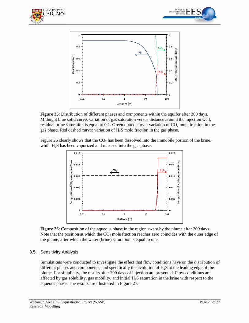
Figure 25, it is inferred that for the base case scenario and after 200 days, the plume radius will be
approximately 35.5 m, of which 27 m belong to first sub-region and the remaining 8.5 m is
considered to be the second sub-region.
Wabamun Area CO2 Sequestration Project (WASP) Page 23 of 27
Reservoir Modelling
Figure 25: Distribution of different phases and components within the aquifer after 200 days.
Midnight blue solid curve: variation of gas saturation versus distance around the injection well,
residual brine saturation is equal to 0.1. Green dotted curve: variation of CO2 mole fraction in the
gas phase. Red dashed curve: variation of H2S mole fraction in the gas phase.
Figure 26 clearly shows that the CO2 has been dissolved into the immobile portion of the brine,
while H2S has been vaporized and released into the gas phase.
Figure 26: Composition of the aqueous phase in the region swept by the plume after 200 days.
Note that the position at which the CO2 mole fraction reaches zero coincides with the outer edge of
the plume, after which the water (brine) saturation is equal to one.
3.5. Sensitivity Analysis
Simulations were conducted to investigate the effect that flow conditions have on the distribution of
different phases and components, and specifically the evolution of H2S at the leading edge of the
plume. For simplicity, the results after 200 days of injection are presented. Flow conditions are
affected by gas solubility, gas mobility, and initial H2S saturation in the brine with respect to the
aqueous phase. The results are illustrated in Figure 27.

Wabamun Area CO2 Sequestration Project (WASP) Page 24 of 27
Reservoir Modelling
(a) Effect of Gas Solubility
The effect of solubility was examined by considering pure water instead of brine. It was
assumed that the initial concentration of H2S was equal to the saturated brine base case.
The higher solubility of the non-hydrocarbon components into the pure water relative to the
brine case causes the ultimate radius of the CO2 plume to shrink, from 35.5 to 34.5 m in the
base case. This indicates less H2S was released from the (sour) pure water case (see
Figure 27-a).
(b) Effect of Gas Mobility
The effect of gas mobility was examined by changing the gas relative permeability and
increasing the end point of gas permeability from 0.4 to 1.0 (Figure 1, Krg [case a]). In the
case of a more adverse mobility ratio (higher gas mobility), the gas spread over a larger
contact area with the aqueous phase (larger radius of plume equalled 42 m), thereby more
effectively stripping H2S away from the brine when in contact with the advancing gas front
(see Figure 27-b).
(c) Effect of Initial Concentration of Dissolved H2S in Brine
Simulations were run for another case where the initial concentration of the dissolved H2S
in the brine was decreased by 25%. Hence, in this case the initial mole fraction of H2S in
the brine was equal to 0.005. The simulation results in Figures 27-c revealed that although
the cumulative mass of released H2S (determined by calculating the area under the graph of
H2S concentration versus distance) is reduced by decreasing the initial concentration of the
dissolved H2S in brine, the mole fraction of released H2S in the gas phase is still high.
These results also illustrate the fact that the initial concentration of H2S has a second-order
effect on the evolution of H2S during CO2 sequestration.
(a)

Wabamun Area CO2 Sequestration Project (WASP) Page 25 of 27
Reservoir Modelling
(b)
(c)
Figure 27: Effect of different parameters on the distribution of different phases and components
beneath the caprock after 200 days: (a) increased gas solubility, (b) increased gas mobility,
(c) decreased initial mole fraction of dissolved H2S in the brine by 25%.

Wabamun Area CO2 Sequestration Project (WASP) Page 26 of 27
Reservoir Modelling
SUMMARY
In this study, we performed numerical modelling of injecting large volumes of CO2 (1 Gt target
over 50 years) into the Nisku Formation. Injection was performed within localized injection areas
of 30 km 60 km. The main objectives of the study were to:
estimate the injection capacity and CO2 plume movement and pressure distribution during
and after injection;
estimate the timescales of the long-term fate of injection associated with free-phase CO2,
aquifer pressurization, and the effect of dip on plume shape and migration; and
assess possible H2S concentration (mole fraction) in the CO2 plume over time and space.
It was shown that the capacity of injection is limited not by available pore space, but by the ability
to inject without exceeding the fracture pressure of the formation. Although capacity increases with
the number of injectors, increasing the number of wells has a limit. Very strong interference
between pressure plumes was observed with no substantial benefit beyond 20 wells. Horizontal
injection wells and aquifer fracturing may be considered as options to increase capacity. Sensitivity
of capacity to reservoir permeability, rock compressibility and well placement was investigated.
The saturation and pressure field simulations show that for multiple injection scenarios (n wells),
CO2 saturation plumes have no interference; we see n individual plumes with a radius of 4 to 5 km
for each injector. The pressure field behaves completely different than the saturation field. There
are no individual pressure plumes, but a single large (scale of hundred km) pressure disturbance.
It was shown that the dip in the Nisku formation does not affect the results (i.e., no substantial
plume movement), although free-phase CO2 may migrate along the dip if it reaches a zone with
higher permeability (above 100 mD). We estimated that at the Nisku conditions, the timescale for
pressure decay is 120 years and the timescale for free-phase CO2 dissolution is ~ 3000 years where
the mechanism of dissolution is natural convection.
An assessment of the possible H2S concentrations in the CO2 plume over time and space was
performed. It showed that H2S dissolved in aquifer brine will be released into the CO2 plume during
injection and will reach a high mole fraction at the outer edge of the CO2 plume.
ACKNOWLEDGMENTS
Financial support for this work was provided by NSERC Strategic Grant and AERI, with additional
funding from industry partners through the Wabamun Area CO2 Sequestration Project (WASP) led
by the University of Calgary. Simulation software (GEM) was donated by the Computer Modelling
Group. This support is gratefully acknowledged. We also wish to thank Long Neighem and Vijay
Shrivastava for their help with the new version of GEM and for the useful discussions of its
applications to this study.

Wabamun Area CO2 Sequestration Project (WASP) Page 27 of 27
Reservoir Modelling
REFERENCES
[1] B. Hitchon, Aquifer Disposal of Carbon Dioxide, Hydrodynamic and Mineral Trapping –
Proof of Concept, 1996, Geoscience Publishing Ltd., Sherwood Park, Alberta, Canada.
[2] H. Hassanzadeh, M. Pooladi-Darvish, A. M. Elsharkawy, D. W. Keith, Y. Leonenko,
Predicting PVT data for CO2-brine mixtures for black-oil simulation of CO2 geological
storage. Int. J. Greenhouse Gas Control, 2008, 2, p. 65–77.
[3] B. Bennion, S. Bachu, Relative permeability characteristics for supercritical CO2 displacing
water in a variety of potential sequestration zones in the western Canada sedimentary basin,
Paper SPE 95547 at SPE Annual Technical Conference an Exhibition, Dallas, TX, p. 9–12
October, 2005.
[4] K. Pruess, J. Garcia, T. Kovscek, C. Oldenburg, J. Rutqvist, C. Steefel, T. F. Xu, Code
intercomparison builds confidence in numerical simulation models for geologic disposal of
CO2, Energy. 2004, 29, p. 1431–1444.
[5] J. M. Nordbotten, M. A. Celia, and S. Bachu, Injection and storage of CO2 in deep saline
aquifers: Analytical solution for CO2 plume evolution during injection. Transport in Porous
Media 2005, 58(3), p. 339–360.
[6] A. Lucier and M. Zoback, Assessing the economic feasibility of regional deep saline aquifer
CO2 injection and storage: A geomechanics-based workflow applied to the Rose Run
sandstone in Eastern Ohio, USA. Int. J. Greenhouse Gas Control, 2008, 2, p. 230–247.
[7] Y. Leonenko and D. W. Keith, Reservoir engineering to accelerate the dissolution of CO2
stored in aquifers, Environmental Science and Technology, 2008, 42(8), p. 2742–2747.
[8] Hassanzadeh, H.; Pooladi-Darvish, M.; Keith, D. W. Stability of a fluid in a horizontal
saturated porous layer: effect of non-linear concentration profile, initial, and boundary
conditions. Transport in Porous Media, 2006, 65, p. 193–211.
[9] Hassan Hassanzadeh, Mehran Pooladi-Darvish, and David W. Keith, Scaling Behavior of
Convective Mixing, with Application to Geological Storage of CO2, AIChE, 2007, Vol. 53,
No. 5, p. 1121–1131.
[10] Nghiem, L.; Sammon, P.; Grabenstetter, J.; Ohkuma, H. Modelling CO2 Storage in Aquifers
with a Fully-Coupled Geochemical EOS Compositional Simulator, SPE Paper No. 89474,
2004.
[11] Harvey, A.H. 1996. Semiempirical correlation for Henry’s constants over large temperature
ranges, AIChE J, Vol. 42, No. 5, p. 1491–1494.
[12] Duan, Z., Sun, R. Liu, R. and Zhu, C., 2007. Accurate thermodynamic model for the
calculation of H2S solubility in pure water and brine. Energy and Fuels, 21, p. 2056–2065.
[13] Kestin, J., Khalifa, H.E., Correia, R.J., 1981. Tables of the dynamic and kinematic viscosity of
aqueous NaCl solutions in the temperature range 20–150°C and pressure range 0.1−35 MPa.
J. Phys. Chem. Ref. Data, Vol. 10, p. 71–87.
[14] Rowe, A.M., Chou, J.C.S., 1970. Pressure-volume-temperature-concentration relation of
aqueous NaCl solutions. J. Chem. Eng. Data, Vol. 15, 1970, p. 61–66.
[15] Corey, A.T., 1954. The interrelation between gas and oil relative permeabilities. Producers
Monthly, November, p. 38–41.