reservoir characterization focus article - arcis.com in northwest louisiana and east texas, ... as...

Some current workflows in shale gas reservoir characterizationSatinder Chopra*, Ritesh K. Sharma* and Kurt J. Marfurt***Arcis Seismic Solutions, TGS, Calgary, Alberta, Canada; **The University of Oklahoma, Norman, Oklahoma, USA

42 CSEG RECORDER September 2013

Continued on Page 43

FOCU

S AR

TICL

E

Summary

With the emergence of the shale gas resources as an importantenergy source, the characterization of mudrocks has gainedsignificance. To be a good resource, mudrocks need to containsufficient organic content and respond effectively to hydraulicfracturing. Variations in total organic carbon, as well as brit-tleness which is a function of mineralogy, influence thecompressional velocity, shear velocity, density and anisotropyof the mud rock. It should therefore be possible to detectchanges in TOC and brittleness from the good quality surfaceseismic data. Besides TOC and brittleness, different shaleformations have different properties in terms of maturation,gas-in-place, and permeability, which with proper calibrationwith well measurements, may be estimated statistically usingsurface seismic data.

Introduction

In the last decade and more, shale gas resources haveemerged as not only a viable but also one of the more signif-icant new energy sources. This viability was first demon-strated using newly perfected methods of hydraulicfracturing and horizontal drilling on the MississippianBarnett Shale in the Fort Worth Basin. Given this initialsuccess, geoscientists began to look for other shale basins inthe US and soon the Devonian Antrim shale of the MichiganBasin, the Devonian Marcellus Shale of the AppalachianBasin, the Devonian New Albany Shale in the Illinois Basinand the Cretaceous Lewis Shale in San Juan Basin wereexplored and developed. Following these, the FayettevilleShale in Arkansas, the Woodford Shale in Oklahoma, theMuskwa Shale in the Horn River Basin, and the MontneyShale, both in British Columbia, Canada, the HaynesvilleShale in northwest Louisiana and east Texas, and the EagleFord Shale in south Texas were developed.

The development of these shales changed the traditionalapproach geologists had been following – that of the sequenceof gas first being generated in the source rock, followed by itsmigration into the reservoir rock in which it is trapped. Shale-gas formations are the source rock, reservoir and seal. There isno need for migration and since the permeability is near zero,it forms its own seal. The gas may be trapped as free gas innatural fractures and intergranular porosity, as gas sorbed intokerogen and clay-particle surfaces, or as gas dissolved inkerogen and bitumen (Curtis, 2002).

Such self-sourcing shale formations are commonly referred toas unconventional shale reservoirs. A more accurate word mightbe mudrock (Hart, 2013), since many shale source rocks do notrespond well to hydraulic fracturing, either because they aretoo ductile, or because they quickly deform about the prop-pant, closing any fractures due to completion. Indeed, theminearology of most commercial shale reservoirs contains

than 50% quartz and/or carbonate. The first thing that werealize in these unconventional shale reservoirs is that theyhave lower permeability than our conventional reservoirs. Itmay not be possible for the hydrocarbons to migrate withinthese formations, and would need stimulation in the form ofhydraulic fracturing so as to release the oil and gas. Secondly,we do not need to map discrete structural and/or stratigraphictraps; these unconventional reservoirs are regionally pervasiveaccumulations. Although pervasive, these reservoirs are notuniform. There are optimal levels in which to land a horizontalwell, TOC and brittleness varies laterally, and geohazards suchas small faults need to be avoided.

To assess the prospectivity of these reservoirs, a criterioncomprising the following elements could be followed:

1. Type of shale: i.e. whether it is a marine or a non-marineshale. Marine shales have low clay-content, are high inbrittle minerals such as quartz, feldspar and carbonatesand so respond better to hydraulic stimulation.

2. Depth: has a bearing on the generated hydrocarbon. Gasfor example, is generated as biogenic gas by the action ofanaerobic micro-organisms during the early burialphase, or as thermogenic breakdown of kerogen atgreater depths and temperatures. Generally, a usefuldepth criterion for shale gas would be between 1000-5000 m. Areas shallower than 1000 m would usuallyhave lower pressures and gas concentrations while areasbelow 5000m often have reduced permeability thattranslates into higher drilling and development costs.

3. Thermal maturity: refers to the degree of heat and the timein the “oven” to which the formation has been exposedresulting in the breakdown of kerogen into hydrocarbons.The indicator for this measure is called vitrinitereflectance and has typical values ranging from 1% to 3%.

4. Total organic carbon (TOC): refers to the organic richnessof the formation in terms of the organic material such asmicroorganism fossils and plant matter that provide thecarbon, oxygen and hydrogen for generating the oil andgas. Typical values are equal to or greater than 1%. TheTOC and thermal maturity of source rocks is assessed bymeans of lab analysis.

5. Permeability: refers to the fluid storage and transmissivitycharacteristics of a shale formation. Shale permeability islow and so artificial stimulation, e.g. hydraulic frac-turing, is required to facilitate the flow of hydrocarbonsinto the well bore. It is important to map the intensityand orientation of natural fractures if they exist in theformation of interest. If open or poorly cemented, stimu-lation will “pop open” these previously generated zonesof weakness. In some cases tightly cemented fracturescan form fracture barriers.

September 2013 CSEG RECORDER 43

Focus Article Cont’dSome current workflows…Continued from Page 42


6. Mineralogy: The mineral composition in shale rock forma-tions can be wide-ranging. In a new area, one shouldattempt to acquire some core for an initial analysis. Electroncapture spectroscopy (ECS) logs provide an initial estimateof mineralogy, but not of the form of the mineral (e.g. gran-ular vs. cryptocrystalline) which also plays a role in brittle-ness behavior. One best practice is to construct a ternarydiagrams of quartz, total clay and total carbonate, and mapit to elastic parameters such as E�(Young’s modulus) andPoisson’s ratio, resulting in a brittleness template. Suchtemplates can then be calibrated to microseismic event loca-tion, production logs, and production itself to assess the brit-tleness or the ductility of the formation and how efficientlythe induced fractures have stimulated it.

7. Fluid in place: is usually calculated from the pressure,temperature, porosity and the TOC for assessing theeconomics of the play.

An optimum combination of these elements leads to favorableproductivity.

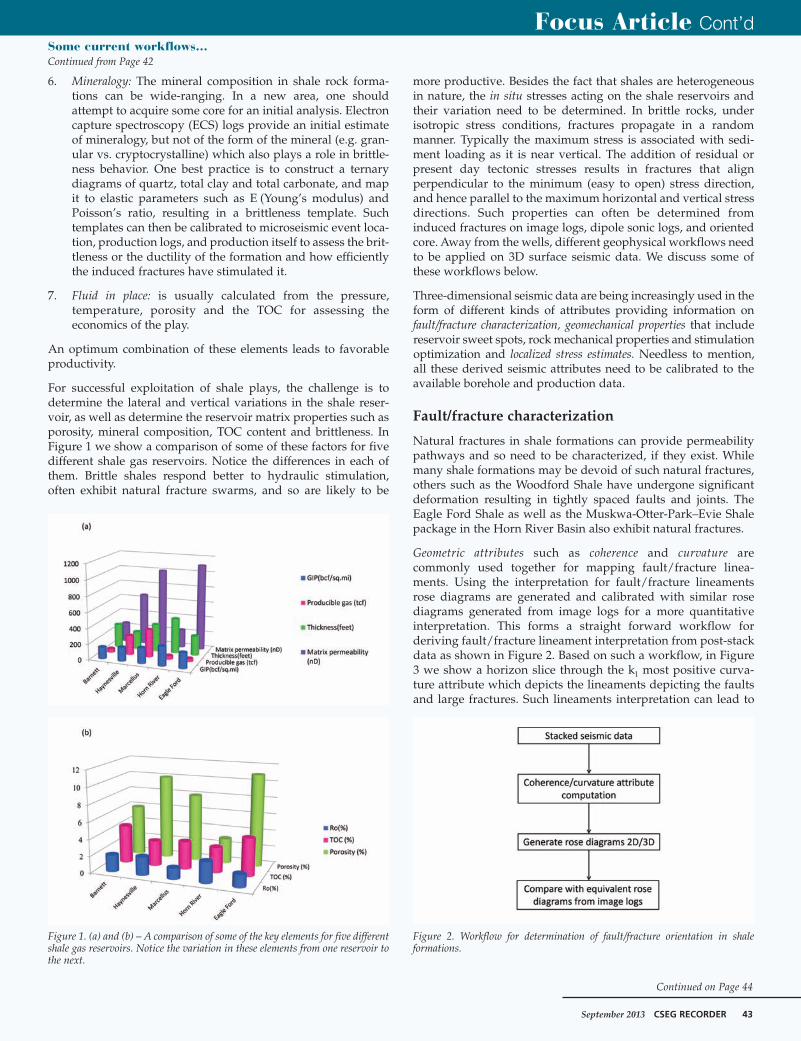
For successful exploitation of shale plays, the challenge is todetermine the lateral and vertical variations in the shale reser-voir, as well as determine the reservoir matrix properties such asporosity, mineral composition, TOC content and brittleness. InFigure 1 we show a comparison of some of these factors for fivedifferent shale gas reservoirs. Notice the differences in each ofthem. Brittle shales respond better to hydraulic stimulation,often exhibit natural fracture swarms, and so are likely to be

more productive. Besides the fact that shales are heterogeneousin nature, the in situ stresses acting on the shale reservoirs andtheir variation need to be determined. In brittle rocks, underisotropic stress conditions, fractures propagate in a randommanner. Typically the maximum stress is associated with sedi-ment loading as it is near vertical. The addition of residual orpresent day tectonic stresses results in fractures that alignperpendicular to the minimum (easy to open) stress direction,and hence parallel to the maximum horizontal and vertical stressdirections. Such properties can often be determined frominduced fractures on image logs, dipole sonic logs, and orientedcore. Away from the wells, different geophysical workflows needto be applied on 3D surface seismic data. We discuss some ofthese workflows below.

Three-dimensional seismic data are being increasingly used in theform of different kinds of attributes providing information onfault/fracture characterization, geomechanical properties that includereservoir sweet spots, rock mechanical properties and stimulationoptimization and localized stress estimates. Needless to mention, all these derived seismic attributes need to be calibrated to theavailable borehole and production data.

Fault/fracture characterization

Natural fractures in shale formations can provide permeabilitypathways and so need to be characterized, if they exist. Whilemany shale formations may be devoid of such natural fractures,others such as the Woodford Shale have undergone significantdeformation resulting in tightly spaced faults and joints. TheEagle Ford Shale as well as the Muskwa-Otter-Park–Evie Shalepackage in the Horn River Basin also exhibit natural fractures.

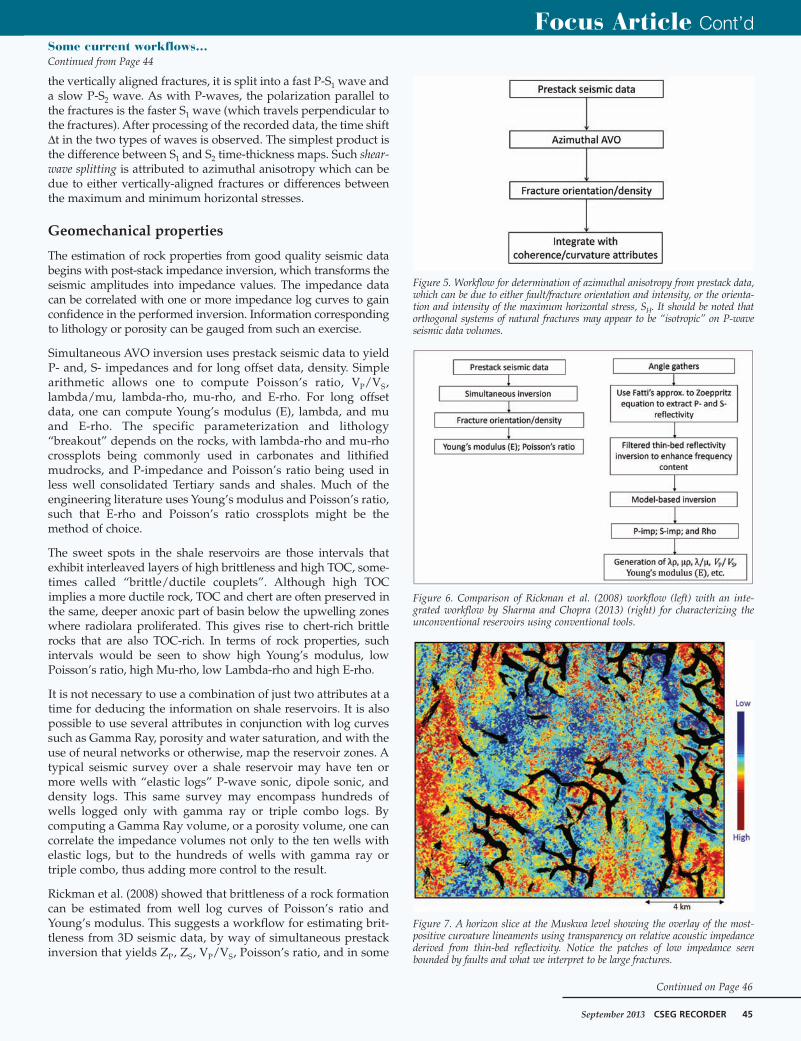
Geometric attributes such as coherence and curvature arecommonly used together for mapping fault/fracture linea-ments. Using the interpretation for fault/fracture lineamentsrose diagrams are generated and calibrated with similar rosediagrams generated from image logs for a more quantitativeinterpretation. This forms a straight forward workflow forderiving fault/fracture lineament interpretation from post-stackdata as shown in Figure 2. Based on such a workflow, in Figure3 we show a horizon slice through the k1 most positive curva-ture attribute which depicts the lineaments depicting the faultsand large fractures. Such lineaments interpretation can lead to

Figure 1. (a) and (b) – A comparison of some of the key elements for five differentshale gas reservoirs. Notice the variation in these elements from one reservoir tothe next.

Figure 2. Workflow for determination of fault/fracture orientation in shaleformations.


rose diagrams or 3D rose diagrams may be generated fromattributes such as the strike of the maximum curvature and theazimuth of minimum curvature (Chopra et al., 2009). In Figure4 we show chair diagrams through k1 most-positive curvature,k2 most-negative curvature, the structural shape-index modu-lated by curvedness and co-rendered with coherence, and the3D rose diagrams from a 3D volume from the Woodford Shale inthe Arkoma Basin of Oklahoma. Notice the different orientationof lineaments as indicated with the yellow arrow pockets ascompared with the background orientation of NE-SW.

Natural vertical fractures, a consequence of the vertical principalstresses or otherwise, gives rise to horizontal transverse isotropy(HTI). Longitudinally polarized P-waves travel faster parallel tothe fractures and slower perpendicular to the fractures, resultingin azimuthal anisotropy. The azimuthal variation in travel timevariation is referred to as velocity vs azimuth (VVAz), while theazimuthal variation in reflection coefficients (amplitude) isreferred to as amplitude variation with azimuth (AVAz). VVAzrequires accurate statics and velocity analysis, does not requireamplitude-preserving processing, and provides vertical resolutionon the formation by formation (velocity picking) scale. AVAzrequires relative amplitude preservation processing. While theoutput is sample by sample, the resolution is more appropriatelyapproximated by the size of the seismic wavelet. Both VVAz andAVAz yield estimates of the orientation (strike) and intensity ofanisotropy. At present, one cannot differentiate betweenanisotropy due to natural fractures and anisotropy due to lateralvariability in horizontal stress (which opens and closes micro frac-tures). In either case, such information comes in handy whenchoosing an optimal orientation for horizontal wells (Treadgold etal. , 2011; Zhang et al., 2010) mapped anisotropy in survey wherethe seismic data were acquired after hydraulic fracturing. Suchsurvey may be used in the future to guide infill drilling to exploitby-passed pay or to restimalate a previously stimulated reservoir.These attributes are derived from the conventional 3D seismicsurveys using only the vertical prestack P-wave componentseismic data and forms a separate workflow as shown in Figure 5.

With multicomponent seismic data, it is possible to add themode-converted P-S waves (downgoing P-wave converting to anupgoing S-wave) to the data mix. As a P-S wave passes through



Figure 4. Vertical slice through the seismic data along line AA’ and horizon slices through volumes of (a) k1 most-positive curvature, (b) k2 most-negative principalcurvature, (c) structural shape-index modulated by curvedness co-rendered with coherence, and (d) 3D rose diagrams. (After Zhang et al., 2010)

Figure 3. A horizon slice at the Muskwa level from the most-positive curvatureattribute. Notice the lineaments on this display which either an appropriate defor-mation model or statistical calibration can serve as a proxy for large fractures.


the vertically aligned fractures, it is split into a fast P-S1 wave anda slow P-S2 wave. As with P-waves, the polarization parallel tothe fractures is the faster S1 wave (which travels perpendicular tothe fractures). After processing of the recorded data, the time shiftDt in the two types of waves is observed. The simplest product isthe difference between S1 and S2 time-thickness maps. Such shear-wave splitting is attributed to azimuthal anisotropy which can bedue to either vertically-aligned fractures or differences betweenthe maximum and minimum horizontal stresses.

Geomechanical properties

The estimation of rock properties from good quality seismic databegins with post-stack impedance inversion, which transforms theseismic amplitudes into impedance values. The impedance datacan be correlated with one or more impedance log curves to gainconfidence in the performed inversion. Information correspondingto lithology or porosity can be gauged from such an exercise.

Simultaneous AVO inversion uses prestack seismic data to yieldP- and, S- impedances and for long offset data, density. Simplearithmetic allows one to compute Poisson’s ratio, VP/VS,lambda/mu, lambda-rho, mu-rho, and E-rho. For long offsetdata, one can compute Young’s modulus (E), lambda, and muand E-rho. The specific parameterization and lithology“breakout” depends on the rocks, with lambda-rho and mu-rhocrossplots being commonly used in carbonates and lithifiedmudrocks, and P-impedance and Poisson’s ratio being used inless well consolidated Tertiary sands and shales. Much of theengineering literature uses Young’s modulus and Poisson’s ratio,such that E-rho and Poisson’s ratio crossplots might be themethod of choice.

The sweet spots in the shale reservoirs are those intervals thatexhibit interleaved layers of high brittleness and high TOC, some-times called “brittle/ductile couplets”. Although high TOCimplies a more ductile rock, TOC and chert are often preserved inthe same, deeper anoxic part of basin below the upwelling zoneswhere radiolara proliferated. This gives rise to chert-rich brittlerocks that are also TOC-rich. In terms of rock properties, suchintervals would be seen to show high Young’s modulus, lowPoisson’s ratio, high Mu-rho, low Lambda-rho and high E-rho.

It is not necessary to use a combination of just two attributes at atime for deducing the information on shale reservoirs. It is alsopossible to use several attributes in conjunction with log curvessuch as Gamma Ray, porosity and water saturation, and with theuse of neural networks or otherwise, map the reservoir zones. Atypical seismic survey over a shale reservoir may have ten ormore wells with “elastic logs” P-wave sonic, dipole sonic, anddensity logs. This same survey may encompass hundreds ofwells logged only with gamma ray or triple combo logs. Bycomputing a Gamma Ray volume, or a porosity volume, one cancorrelate the impedance volumes not only to the ten wells withelastic logs, but to the hundreds of wells with gamma ray ortriple combo, thus adding more control to the result.

Rickman et al. (2008) showed that brittleness of a rock formationcan be estimated from well log curves of Poisson’s ratio andYoung’s modulus. This suggests a workflow for estimating brit-tleness from 3D seismic data, by way of simultaneous prestackinversion that yields ZP, ZS, VP/VS, Poisson’s ratio, and in some

Focus Article Cont’dSome current workflows…Continued from 4


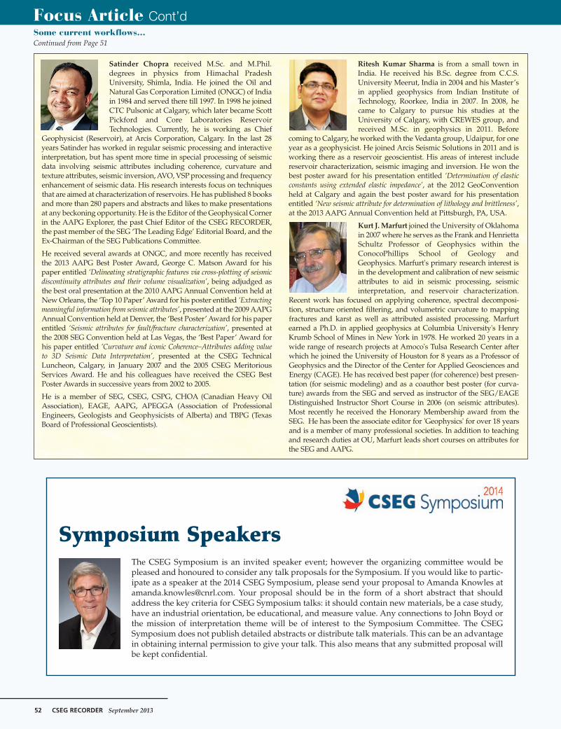
Figure 7. A horizon slice at the Muskwa level showing the overlay of the most-positive curvature lineaments using transparency on relative acoustic impedancederived from thin-bed reflectivity. Notice the patches of low impedance seenbounded by faults and what we interpret to be large fractures.

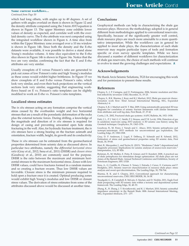
Figure 6. Comparison of Rickman et al. (2008) workflow (left) with an inte-grated workflow by Sharma and Chopra (2013) (right) for characterizing theunconventional reservoirs using conventional tools.

Figure 5. Workflow for determination of azimuthal anisotropy from prestack data,which can be due to either fault/fracture orientation and intensity, or the orienta-tion and intensity of the maximum horizontal stress, SH. It should be noted thatorthogonal systems of natural fractures may appear to be “isotropic” on P-waveseismic data volumes.


cases meaningful estimates of density. Zones with high Young’smodulus and low Poisson’s ratio are those that would be brittleas well as have better reservoir quality (higher TOC, higherporosity). Such a workflow works well for good quality data andis shown in Figure 6.

A somewhat different workflow was described by Sharma andChopra (2013), that results in enhanced resolution of the deriveddata attributes and hence the desired detail in terms of accuratesweet spot detection. This workflow begins with the anglegathers derived from conditioned offset gathers, from which theP- and S-reflectivity data is derived using Fatti’s approximationsto the Zoeppritz equations. A density attribute can also bederived but depends on the quality of the input data as well asthe presence of long offsets. Thin-bed reflectivity inversion(Chopra et al., 2006) is now utilized for enhancing the resolutionof the P- and S-reflectivity data wherein the effect of the wavelet

is removed from the data and the output of the inversion processcan be viewed as spectrally broadened seismic data, retrieved inthe form of broadband reflectivity data that can be filtered backto any bandwidth. This usually represents useful information forinterpretation purposes. Since thin-bed reflectivity removes theseismic wavelet and better estimates a suite of reflection spikes,it better honors the assumptions of “trace integration” relativeacoustic impedance. Furthermore, the absence of the seismicwavelet provides a relative acoustic impedance volume that hasa higher level of detail. In Figure 7 we show a horizon sliceoverlay of a k1 most-positive principal curvature volume seen asblack lineaments using transparency with an equivalent slicethrough the relative acoustic impedance derived from P-reflec-tivity volume. We notice some patches of low impedance seenbounded by faults and large fracture lineaments. In Figure 8 weshow an overlay of the fracture network lineaments using trans-

parency over the relativeimpedance derived fromreflectivity, (a) before, and (b)after frequency enhancement.Notice the different curvaturelineaments appear to fall intothe appropriate high imped-ance pockets separating themfrom low impedance pockets,which may be suggestingcemented fractures.

Similarly, the differencebetween the Rickman et al.(2008) workflow and theproposed workflow by Sharmaand Chopra (2013) is demon-strated in terms of a verticalsection comparison as well as atime slice comparison in Figures9 and 10. The data are takenfrom the lambda-rho volumesgenerated by both the work-flows. Notice the extra level ofdetail seen in the proposedworkflow.



Figure 8. Horizon slices through the acoustic impedance volumes (a) before, and (b) after frequency enhancement, at a levelwithin the Montney shale in NE British Columbia, Canada. Note, at places there is correlation between low-impedanceanomalies (blue) and the presence of curvature lineaments. At other places there is no correlation (highlighted in blue dottedellipses).

Figure 9. Segment of a lambda-rho section from the (a) Rickman et al. (2008) workflow, and (b) proposed workflow. Notice the increased level of detail seen in (b) due to theenhance resolution employed in the proposed workflow.


Next, the output of thin-bed inversion is considered as input forthe model based inversion to compute P-impedance, S-imped-ance and density, which in turn are used to compute other rele-vant attributes, such as the lr, mr and VP/VS. These can be usedto estimate the pore space properties and other informationabout the rock skeleton. Young’s modulus can be treated as abrittleness indicator and Poisson’s ratio as TOC indicator.

Sharma and Chopra (2013) have demonstrated the generation ofE-rho attribute following the integrated workflow shown inFigure 6, and demonstrated that the E-rho curve computed fromthe log data and compared with the Mu-rho curve shows ahigher level of detail. We elaborate on this attribute a little morehere. As shown in Figure 11, the computed E-rho curve looksvery similar to the E curve. One can cross-correlate these twocurves and study their similarity, which in this case showedmaximum correlation at zero lag and so high similarity. In anattempt to demonstrate this on real seismic data, we picked up adataset from the Montney area in NE British Columbia, Canada,



Figure 12. Angle information in colour overlaid on seismic gathers. The range ofangles selected for density inversion is up to 49 degrees.

Figure 11. Display of log curves as well as the derived curves E and E-rho for abroad zone of interest covering the Lower and Upper Montney Formation in BritishColumbia, Canada. As we notice, the E and E-rho curves are very similar.

Figure 10. Horizon slice at a level 30 ms below the Montney marker and averaged in a 10 ms window, from the lambda-rho volumes derived using (a) Rickman et al.(2008) workflow, and (b) proposed workflow.

Figure 13. A representative section from the density volume computed fromsimultaneous inversion. Low values of density are seen in the Upper MontneyFormation, and the overlaid density curve also shows good correlation.




Figure 14. Time slices from within the Upper Montney Formation averaged over a 10 ms window from (left) the Young’s modulus (E) volume, and (right) the E-rho volume.Apparently, the two are very similar.

Figure 15. Crossplots between (left) E and Poisson’s ratio and (right) E - rho over a zone that includes the Upper Montney Formation. Notice the similarity between thecluster points. Back projection of points selected by polygons in the figure above on the vertical seismic are show below. Again notice that the two patterns are very similar.


which had long offsets, with angles up to 49 degrees. A set ofgathers with angles overlaid on them is shown in Figure 12 andthe density attribute computed using the 3-term AVO equation isshown in Figure 13. The upper Montney zone exhibits lowervalues of density as expected, and correlate well with the over-laid density curve. The E-rho attribute was next computed usingthe integrated workflow shown in Figure 6. A time slice fromwithin the Upper Montney zone averaged over a 10 ms windowis shown in Figure 14b. Since both the density and the E-rhodatasets were available, it was possible to derive a stand aloneYoung’s modulus volume. A time slice equivalent to the E-rhoslice shown in Figure 14b is shown in Figure 14a. Notice that thetwo are very similar, confirming the fact that the E and E-rhoattributes are very similar.

Usually crossplots of E versus Poisson’s ratio are generated topick out zones of low Poisson’s ratio and high Young’s modulusas these zones would exhibit higher brittleness. In Figure 15 weshow crossplots of E and E-rho versus Poisson’s ratio, whichlook very similar, and even their back projections on the verticalsections look very similar, suggesting that engineering work-flows based on E vs. Poisson’s ratio templates can be slightlymodified to work on E-rho vs. Poisson’s ratio templates.

Localized stress estimates

The in situ stresses acting on any formation comprise the verticalstress caused by the overburden weight and two horizontalstresses that are a result of the poroelastic deformation of the rocksplus the external tectonic forces. During drilling, a knowledge ofthe magnitude and direction of in situ stresses is required fordesign of casing and preventing unwanted open hole strata fracturing in the well. Also, for hydraulic fracture treatment, the insitu stresses have a strong bearing on the fracture azimuth andorientation, fracture width, height, its growth and its conductivity.

These in situ stresses can be estimated from the geomechanicalproperties determined from seismic data as discussed above. Inparticular two attributes, namely the differential horizontal stressratio (Gray et al., 2012; Sena et al., 2011) (DHSR) and closure stress(Goodway et al., 2010) are commonly used for the purpose.DHSR is the ratio between the maximum and minimum hori-zontal stresses to the maximum horizontal stress. Zones with lowDHSR values, could have fractures formed in a random mannerand so creating a fracture swarm. Thus low DHSR values arefavorable. Closure stress is the minimum pressure required tohold open a fracture once it is created. Optimal producing zoneswould exhibit high Young’s modulus and low DHSR or closurestress values. The derivation of stress estimates from some of theattributes discussed above would be discussed at another time.

Conclusions

Geophysical methods can help in characterizing the shale gasresource plays. However, the methodology adopted is in generaldifferent from methodologies applied to conventional reservoirs.Specifically, because of the significantly greater well control,shale resource plays are much more amenable to a more quanti-tative interpretation. While the workflows can in general beapplied to most shale plays, the characterization of each shalereservoir may require particular types of tools and formationspecific or even survey specific templates. While we havediscussed a number of different workflows for characterizationof shale gas reservoirs, the choice of such methods will continueto evolve to meet the growing challenges and expectations. R

Acknowledgements

We thank Arcis Seismic Solutions, TGS for encouraging this workand for permission to present these results.

ReferencesChopra, S., J. P. Castagna, and O. Portniaguine, 2006, Seismic resolution and thin-bed reflectivity inversion: CSEG Recorder, 31, 19–25.

Chopra, S., R.K. Sharma, J. Keay and K.J. Marfurt, 2012, Shale gas reservoir charac-terization work flow: 82nd Annual International Meeting, SEG, ExpandedAbstracts,1-4.

Chopra, S, K. J. Marfurt and H. T. Mai, 2009, Using automatically generated 3D rosediagrams for correlation of seismic fracture lineaments with similar lineamentsfrom attributes and well log data, First Break, 27, 37-42

Curtis, J. B., 2002, Fractured shale gas systems: AAPG Bulletin, 86, 1921–1938.

Fatti, J. L., P. J. Vail, G. C. Smith, P. J. Strauss, and P. R. Levitt, 1994, Detection of gasin sandstone reservoirs using AVO analysis: A 3D seismic case history using theGeostack technique: Geophysics, 59, 1362–1376.

Goodway, B., M. Perez, J. Varsek and C. Abaco, 2010, Seismic petrophysics andisotropic-anisotropic AVO methods for unconventional gas exploration, TheLeading Edge, 29, 1500-1508.

Gray, D. P. Anderson, J. Logel, F. Delbecq, D. Schmidt and R. Schmid, 2012,Estimation of stress and geomechanical properties using 3D seismic data, FirstBreak, 30, 59-68.

Hart, B., Macquaker, J., and Taylor, K. (2013). “Mudstone (“shale”) depositional anddiagenetic processes: Implications for seismic analyses of source-rock reservoirs.”Interpretation, 1(1), B7-B26.

Rickman, R., M. Mullen, E. Petre, B. Grieser, and D. Kundert, 2008, A practical useof shale petrophysics for stimulation design optimization: All shale plays are notclones of the Barnett Shale: Annual Technical Conference and Exhibition, Society ofPetroleum Engineers, SPE 11528.

Sena, A., G. Castillo, K. Chesser, S. Voisey, J. Estrada, J. Caruz, E. Carmona and P.Hodgkins, 2011, Seismic reservoir characterization in resource shale plays: stressanalysis and sweet spot discrimination, The Leading Edge, 30, 758-764.

Sharma, R. K. and S. Chopra, 2013, Conventional approach for characterizingunconventional reservoirs, CSEG RECORDER, 38, 34-38.

Treadgold, G., B. Campbell, B. McLain, S. Sinclair, and D. Nicklin, 2011, Eagle Fordshale prospecting with 3D seismic data within a tectonic and depositional systemframework: The Leading Edge, 30, 48–53.

Zhang, K., B. Zhang, J. T. Kwiatkowski, and K. J. Marfurt, 2010, Seismic azimuthalimpedance anisotropy in the Barnett Shale: 80th Annual International Meeting,SEG, Expanded Abstracts, 273 – 277.





Satinder Chopra received M.Sc. and M.Phil.degrees in physics from Himachal PradeshUniversity, Shimla, India. He joined the Oil andNatural Gas Corporation Limited (ONGC) of Indiain 1984 and served there till 1997. In 1998 he joinedCTC Pulsonic at Calgary, which later became ScottPickford and Core Laboratories ReservoirTechnologies. Currently, he is working as Chief

Geophysicist (Reservoir), at Arcis Corporation, Calgary. In the last 28years Satinder has worked in regular seismic processing and interactiveinterpretation, but has spent more time in special processing of seismicdata involving seismic attributes including coherence, curvature andtexture attributes, seismic inversion, AVO, VSP processing and frequencyenhancement of seismic data. His research interests focus on techniquesthat are aimed at characterization of reservoirs. He has published 8 booksand more than 280 papers and abstracts and likes to make presentationsat any beckoning opportunity. He is the Editor of the Geophysical Cornerin the AAPG Explorer, the past Chief Editor of the CSEG RECORDER,the past member of the SEG ‘The Leading Edge’ Editorial Board, and theEx-Chairman of the SEG Publications Committee.

He received several awards at ONGC, and more recently has receivedthe 2013 AAPG Best Poster Award, George C. Matson Award for hispaper entitled ‘Delineating stratigraphic features via cross-plotting of seismicdiscontinuity attributes and their volume visualization’, being adjudged asthe best oral presentation at the 2010 AAPG Annual Convention held atNew Orleans, the ‘Top 10 Paper’ Award for his poster entitled ‘Extractingmeaningful information from seismic attributes’, presented at the 2009 AAPGAnnual Convention held at Denver, the ‘Best Poster’ Award for his paperentitled ‘Seismic attributes for fault/fracture characterization’, presented atthe 2008 SEG Convention held at Las Vegas, the ‘Best Paper’ Award forhis paper entitled ‘Curvature and iconic Coherence–Attributes adding valueto 3D Seismic Data Interpretation’, presented at the CSEG TechnicalLuncheon, Calgary, in January 2007 and the 2005 CSEG MeritoriousServices Award. He and his colleagues have received the CSEG BestPoster Awards in successive years from 2002 to 2005.

He is a member of SEG, CSEG, CSPG, CHOA (Canadian Heavy OilAssociation), EAGE, AAPG, APEGGA (Association of ProfessionalEngineers, Geologists and Geophysicists of Alberta) and TBPG (TexasBoard of Professional Geoscientists).

Ritesh Kumar Sharma is from a small town inIndia. He received his B.Sc. degree from C.C.S.University Meerut, India in 2004 and his Master’sin applied geophysics from Indian Institute ofTechnology, Roorkee, India in 2007. In 2008, hecame to Calgary to pursue his studies at theUniversity of Calgary, with CREWES group, andreceived M.Sc. in geophysics in 2011. Before

coming to Calgary, he worked with the Vedanta group, Udaipur, for oneyear as a geophysicist. He joined Arcis Seismic Solutions in 2011 and isworking there as a reservoir geoscientist. His areas of interest includereservoir characterization, seismic imaging and inversion. He won thebest poster award for his presentation entitled ‘Determination of elasticconstants using extended elastic impedance’, at the 2012 GeoConventionheld at Calgary and again the best poster award for his presentationentitled ‘New seismic attribute for determination of lithology and brittleness’,at the 2013 AAPG Annual Convention held at Pittsburgh, PA, USA.

Kurt J. Marfurt joined the University of Oklahomain 2007 where he serves as the Frank and HenriettaSchultz Professor of Geophysics within theConocoPhillips School of Geology andGeophysics. Marfurt's primary research interest isin the development and calibration of new seismicattributes to aid in seismic processing, seismicinterpretation, and reservoir characterization.

Recent work has focused on applying coherence, spectral decomposi-tion, structure oriented filtering, and volumetric curvature to mappingfractures and karst as well as attributed assisted processing. Marfurtearned a Ph.D. in applied geophysics at Columbia University's HenryKrumb School of Mines in New York in 1978. He worked 20 years in awide range of research projects at Amoco's Tulsa Research Center afterwhich he joined the University of Houston for 8 years as a Professor ofGeophysics and the Director of the Center for Applied Geosciences andEnergy (CAGE). He has received best paper (for coherence) best presen-tation (for seismic modeling) and as a coauthor best poster (for curva-ture) awards from the SEG and served as instructor of the SEG/EAGEDistinguished Instructor Short Course in 2006 (on seismic attributes).Most recently he received the Honorary Membership award from theSEG. He has been the associate editor for 'Geophysics' for over 18 yearsand is a member of many professional societies. In addition to teachingand research duties at OU, Marfurt leads short courses on attributes forthe SEG and AAPG.

Symposium SpeakersThe CSEG Symposium is an invited speaker event; however the organizing committee would bepleased and honoured to consider any talk proposals for the Symposium. If you would like to partic-ipate as a speaker at the 2014 CSEG Symposium, please send your proposal to Amanda Knowles [email protected]. Your proposal should be in the form of a short abstract that shouldaddress the key criteria for CSEG Symposium talks: it should contain new materials, be a case study,have an industrial orientation, be educational, and measure value. Any connections to John Boyd orthe mission of interpretation theme will be of interest to the Symposium Committee. The CSEGSymposium does not publish detailed abstracts or distribute talk materials. This can be an advantagein obtaining internal permission to give your talk. This also means that any submitted proposal willbe kept confidential.

reservoir characterization focus article - arcis.com in northwest louisiana and east texas, ... as...

Documents