research proposal: an experimental investigation of
TRANSCRIPT

Research Proposal:
An Experimental Investigation of Product Di↵erentiation and
Price Competition in the Presence of Network E↵ects
⇤
Fernando Pigeard de Almeida Prado,† Guilherme Valle Moura‡, and Israel Waichman§
19 de fevereiro de 2014
Abstract
Keywords: Product di↵erentiation, network e↵ect, social interactions.
JEL Classification codes: D11, D4, M30
⇤This research was supported by the Sao Paulo Research Foundation (FAPESP) University de SaoPaulo, DCM/FFCLRP, Brazil.
†Departamento de Computacao e Matematica, FFCLRP, Universidade de Sao Paulo, Av. Bandeiran-tes, 3900, CEP 14040-901, Brazil. E-mail: [email protected].
‡Departmento de Economia, Universidade Federal de Santa Catarina, Campus Universit ario TrindadeFlorian opolis/SC, 88049-970 , Brazil. E-mail: [email protected]
§Department of Economics, University of Heidelberg, Bergheimerstrasse 20, 69115, Heidelberg, Ger-many. Email: [email protected]
1

1 Introduction
This proposed research project deals with oligopoly under network e↵ects. Such a
situation was demonstrated by Becker (1991, p.1109): “A popular seafood restaurant in
Palo Alto, California, does not take reservations, and every day it has long queues for
tables during prime hours. Almost directly across the street is another seafood restaurant
with comparable food, slightly higher prices, and similar service and other amenities. Yet
this restaurant has many empty seats most of the time.” In this example consumers have
satisfaction from eating in a popular place where many others are eating. In other words,
the market demand is not determined solely by the prices of the food but also by the size
of the group entering one restaurant or another (i.e., aggregate demands).
Inspired by this case, de Almeida Prado et al. (2011) and de Almeida Prado (2013)
developed a model where they suggest that the polarization of demands discussed for
example by Becker (1991) is a consequence of the proximity of restaurants which in its
turn follows from strong network e↵ects on consumers’ decisions. The explanation for
such a behavior goes as follows: when firms do not di↵erentiate products, the only factors
determining individual choices are di↵erences in aggregate demands. In this case, network
e↵ects lead to herd behavior and a polarization of demand is expected to happen. Further
result of the model is that the market leader (i.e., the firm with the largest market
share) can take advantage of its position and charge a higher price than it’s markets
follower while still maintaining to keep all their consumers (this is also consistent with
Mitchell and Skrzypacz, 2006). If the network e↵ect is su�ciently strong, the market
leader’s price turn to be much higher than the equilibrium price, which is predicted
in case where players separate and share the market symmetrically. Since each firm is
equally likely to become the market leader, their expected profits may be higher when
they agglomerate and fight for the market leadership rather than separate and share
the market symmetrically. Conversely, firms tend to separate and engage in a standard
2

Hotelling price competition when their network e↵ects are su�ciently weak. That may
explain the agglomeration of firms where consumers put high value in socializing with
other consumers (e.g., bars, restaurants, night clubs); and the dispersion of firms in which
consumers are primarily interested in accessing the product (e.g., drug stores, bakeries).
It is very di�cult to find situations in the business world that corresponds exactly to
the theoretical model. Even in the restaurant case that inspired the research some of the
assumptions may not be varied or fulfilled. In this respect, laboratory experiments allow
to specify an environment and define the institutions to be used. Thus, they provide an
opportunity to test descriptiveness of models even under “strong” theoretical assumpti-
ons that are hardly observed in the business world. It is, therefore, hardly surprising
that models of oligopoly were among the first experiments conducted in economics (e.g.,
Sauermann and Selten, 1959; Hoggatt, 1959; Fouraker and Siegel, 1963).
The aim of this research project is to test the prediction of price completion models in
the presence of network e↵ects (see Cabral, 2011 for a review) as well the location/price-
setting model by de Almeida Prado (2013). Moreover, there are several additional reasons
why we want to investigate location- and price-setting dynamics under network e↵ects:
First, although price competition is an issue of major interest in economics and has been
subject to large experimental research (see, for example, Engel, 2007 and Potters and
Suetens, 2013), there is very limited experimental evidence on price competition under
network e↵ects or demand inertia (Keser, 1993, 2000; Bayer and Chan, 2007). We plan
to complement the previous work by (i) testing the isolated e↵ect of network on firms’
collusion, and also (ii) the impact of non binding communication between the firms on
collusion. Second, previous experimental findings are not in line with equilibrium predic-
tions, and the results by Bayer and Chan (2007) are qualitatively di↵erent from Keser
(2000). However, results from a pre-test experiment that we have recently conducted
(see section 5) indicate that our results are much closer to the theoretical prediction than
3

previous studies. Thus, our contribution may be especially important as it may shed light
on topic with ambiguous evidence and also show that theory may be good predictor of
behavior even under competition with network e↵ect (or demand inertia). Third, we in-
troduced a computational tool that may be especially suitable in such experiments where
optimal pricing strategy could vary over time. Thus, we intend to contribute methodo-
logically to the design of further experiment on network externalities. Finally, we intend
to contribute to the literature by being the first to test the e↵ect of network (or demand
inertia) in a location-setting model.
The paper is organized as follows: In Section 2 we describe the theoretical location-
price model with network e↵ect that is the basis for our experimental investigation. In
Section 3 we describe the previous related literature. In Section 4 we portray the pro-
posed experimental design, and Section 5 presents results from a pre-test conducted in
September 2013.
2 Theoretical Model
This section portrays the theoretical model and results by de Almeida Prado (2013)
to be tested experimentally. We introduce a location-price game between two firms (e.g.,
restaurants), which compete for socially interacting consumers distributed along a mea-
surable spatial space (conveniently, a circle of circumference 1). The firms di↵erentiate
their products as they choose their geographic locations along the address space of con-
sumers. Consumers decide simultaneously on the firm they consume from according to
a Hotelling-type utility function, in which individual utility increases in the number of
consumers of the firm under consideration. In equilibrium the distance between firms
depends on the strength of positive network e↵ect in consumers’ decisions and on the
transportation costs of consumers. Assuming quadratic transportation costs as in D’ As-
4

premont et al. (1979), we derive the following results. On the one hand, if the strength of
network e↵ect among consumers is larger than a critical value, then the distance between
firms is zero. On the other hand, if it is lower than this critical value, then the distance
between firms is maximal in Nash equilibrium. The latter corresponds to the standard
result of D’ Aspremont et al. (1979), who does not assume social interactions among
consumers.
2.1 Model
Consumers’ interactions. We consider a model in which consumers are uniformly
distributed along a circular address space1 N of circumference 1. There are two firms, 1
and 2, located at circle points l(1) and l(2). Both firms sell the same physical good. As
in d’Appremont et al. (1979) we assume that transportation costs are quadratic, i.e., a
consumer living at x 2 N incurs a quadratic transportation cost ⌫d2(x, l(i)) to go to firm
i (i 2 {1, 2}), where ⌫ is a positive model parameter, and d(x, l(i)) denotes the shortest
distance between x and l(i) along the circle.
For simplicity in exposition we assume that each consumer purchases one unit of the
good either from firm 1 or firm 2. We denote by N (i) the set of consumers that buy the
good from firm i 2 {1, 2}. Since N = N (1) [ N (2), N (1) describes the configuration of
consumers’ decisions.
We now assume that consumers’ x gross utility from consumption depends on other
consumers’ decisions. If x buys the good from firm i, then x’s gross utility is
J |N (i)| (i 2 {1, 2}) (1)
1Circular address spaces, originally due to Salop (1979), are very common in the literature (Novshek(1980), Eaton and Wooders (1985), Kats (1995), Pal (1998) and Gupta et. all (2006)). We choose acircular address space for simplicity in exposition. Analogous results can be derived by considering theinterval [0, 1].
5

where J is a positive parameter, and |N (i)| denotes the normalized one-dimensional Lebes-
gue measure of N (i) along the circle, where we suppose that N (i), i 2 {1, 2} are Lebesgue
measurable subsets of N . (If N (i) is path connected, then N (i) is an arc on the circle N ,
and |N (i)| is the length of the arc divided by the total circumference 2Dmax
).
If consumer x chooses firm i 2 {1, 2}, his/her net utility is
U (x)(i, |N (i)|) = J |N (i)|� P (i) � ⌫h
d�
x, l(i)�
i2
(2)
where P (i) denotes the price charged by firm i.
We introduce below a location-price game of firms under positive externalities of con-
sumers, that is, under J > 0. Although consumers’ utility depends on other consumers
decisions, it is worth stressing that only the firms 1 and 2 are players of the location-price
game. Consumers just react simultaneously to prices and other consumers’ decisions in
accordance to (2).
Each firm’s i strategy is composed by an initial location l(i), which is chosen at time
t = 0, and a sequence of non-negative prices, which are played on the subsequent times
t = 1, 2, . . . Each price at time t, denoted by P(i)t
(i = 1, 2) is a function of the game
history Ht
(defined below).
The payo↵ of firm i, denoted by ⇧(i)�
(l(1), P (1)); (l(2), P (2))�
, is the expected average
profit over time, where the firm costs are zero:
⇧(i)�
(l(1), P (1)); (l(2), P (2))�
= E(⇡(i)), ⇡(i) = limT!1
1
T
T
X
t=1
�
�N(i)t
�
� ·P (i)t
(i = 1, 2) (3)
Above, E denotes the mathematical expectation operator, and N(1)t
and N(2)t
denote the
sets of consumers that choose firms 1 and 2 at time t, respectively.
The game history Ht
available for both players to choose their prices P (1)t
and P(2)t
at
time t = 1, 2, . . ., is
6

Ht
= l when t = 1, and Ht
= (l, P1, N1, P2, N2, . . . Pt�1, Nt�1) when t > 1
where l = (l(1), l(2)), Pt
= (P (1)t
, P(2)t
) and Nt
= (N (1)t
, N(2)t
).
In order to specify completely the payo↵ functions ⇧(i), we define below how consumers
decisions (determined by sets N (1)t
and N(2)t
) evolve in time.
Dynamics of consumers’ decisions. First of all, we assume that (|N (1)0 |, |N (2)
0 |) is
random. More specifically, we assume that
|N (1)0 | is uniformly distributed over the interval [0, 1] (4)
and |N (2)0 | = 1� |N (1)
0 |.
The vector (|N (1)0 |, |N (2)
0 |) stands for the consumers initial expectation about the real
demand to be formed at time t = 1. This initial market share (expectation) is not observed
by the two players (the firms) when they choose their initial prices P (i)1 , i = 1, 2.
For t = 1, 2, . . ., we assume that consumers are “myopic” rather than fully rational in
the sense that they choose simultaneously best individual responses to other consumers’
expected decisions E(|N (1)t
|) and E(|N (2)t
|) (where |N (1)t
| and |N (2)t
| are not observed by
the consumers at time t) and the observed prices P (1)t
, P(2)t
. As a simple rule of common
expectation, we assume that E(|N (1)t
|), E(|N (2)t
|) = (|N (1)t�1|, |N
(2)t�1|).
Let us denote by i(x)t
(2 {1, 2}) the decision of consumer x at time t � 1. In light of
the consumers’ utility function (2), we set i(x)t
= argmaxi2{1,2} U
(x)t
(i, |N (i)t�1|),2 where
U(x)t
(i, |N (i)t�1|) = J |N (i)
t�1|� P(i)t
� ⌫h
d�
x, l(i)�
i2
(5)
It is straightforward to show recursively that N (i)t
, i = 1, 2, t = 1, 2, . . . are Lebesgue
measurable sets. Indeed, the numbers |N (1)0 |, |N (2)
0 | are well defined. Now, once we have
2When argmaxi2{1,2} U (x)
t
(i, |N (i)t�1|) is multivalued, we set i(x)
t
= 1 without loss of generality.
7

that |N (1)t�1| and |N (2)
t�1| are well defined, it is easy to see that N (i)t
= {x | i(x)t
= i} is an arc
on the circle N , and thus Lebesgue measurable (i = 1, 2). Since |N (1)t
| + |N (2)t
| = 1, the
dynamics of |N (1)t
| and |N (2)t
| are uniquely determined by that of mt
def= |N (1)
t
|� |N (2)t
|.
Dynamics of (mt). Let D be the distance between firms on the address space of
consumers. Tanking into account that the consumers are uniformly distributed over the
circle N , a straightforward calculation shows that
mt
= (mt�1, ht
), where (m,h) =
8
>
>
>
>
>
>
>
>
>
>
<
>
>
>
>
>
>
>
>
>
>
:
�1, if m h��
J
,
J
�
m� h
�
, if h��
J
< m < h+�
J
,
1, if m � h+�
J
,
(6)
and
ht
= P(1)t
� P(2)t
and � = ⌫D(1�D) with 0 D 1/2.3 (7)
Remark. Since |N (1)t
| = (1 +mt
)/2, |N (2)t
| = (1 �mt
)/2 for t > 0, equations (3), (4),
(6), and (7) defines the game. These equations could be used to test the model for finite
time horizon T .
2.2 Results
Below we present some Nash equilibria of the price competition that occurs after
location are fixed. We also solved the overall game applying a backward induction on
the location of firms based on the presented outcomes of the price competition. Under
some technical conditions, the presented outcomes of the price subgame is unique. These
3Since N (the adress space of consumers) is a circle of circunference 1, D is the shortest arc betweenthe firm locations in N , where 0 D 1/2.
8

conditions essentially ensures that players play a convergent price sequence and stop
monitoring the game history after some strategic time.
2.2.1 Nash equilibria of the price competition
Let us assume that the firms have already fixed their locations along the circle. The
proposition below presents a set of Nash equilibria, of which limit prices and payo↵s are
uniquely determined by the distance between firms.
Proposition 1. Let � = ⌫D(1 � D), where D denotes the minimal distance between
firms along the circle. Let us consider the price game of firms 1 and 2 with payo↵ func-
tions ⇧(i)�
(l(1), P (1)); (l(2), P (2))�
, i = 1, 2, defined in (3). The price game (for fixed firm
locations l(1) and l(2)) always has a Nash equilibrium.
Moreover, if (P (1), P (2)) is a Nash equilibrium of the price subgame and |N (i)t
| and
⇧
(i)t
are the values of |N (i)t
| and ⇧(i) in ( P (1), P (2)), then the following conditions hold:
(Duopoly equilibrium) If 0 < J < �, then the following three conditions are satisfied:
1. The firms play the same long run price, and it is
limt!1
P (i)t
= � � J, i = 1, 2 (8)
2. The market is shared symmetrically in the long run, i.e.,
limt!1
| N (i)t
| = 1/2, i = 1, 2 (9)
3. Both players receive the same payo↵, i.e.,
⇧
(i) = (� � J)/2, i = 1, 2 (10)
9

(Monopoly equilibrium) If 0 � J , then the following conditions are satisfied:
1. Firms play the minimum price to attract demand. As soon as one firm monopolizes
the market, it increases its price up to J � �:
P (i)t�1 =
8
>
>
>
>
<
>
>
>
>
:
0 if | N (i)t
| < 1
J � � if | N (i)t�1| = 1
(11)
2. If [0 � < J ] then
Prob⇣
limt!1
|N (i)t
| = 1⌘
=1
2, i 2 {1, 2} (12)
(Each player polarizes the market with probability 12).
3. Both players receive the same (expected) payo↵
⇧
(i) = (J � �)/2, i = 1, 2 (13)
where (13) follows immediately from (11) and (12).
2.2.2 Backward induction on the distance between firms
We now solve the overall game by applying a backward induction on �, which is an
increasing function of the distance between firms D. (The bijection between D and � is
presented in equation (7)). Taking into account Equations (10) and (13), the payo↵s of
players (as a function of �) is ⇧
(i)(�) = |J � �|/2 for 0 � �max
, where �max
= ⌫/4
and |J � �| denotes the absolute value J � �. Maximizing ⇧
(i)(�) yields the equilibrium
values of � (and D). The next proposition present the overall solution of the game.
10

Proposition 2. Set �max
= ⌫/4. Let�
l(1), P (1)); (l(2),P (2))�
be a Nash equilibrium of
the location-price game with payo↵ functions (3). Let � depend on the distance between
locations l(1) and l(2) as defined in (7)). Then � 2 �(J), where
�(J) =
8
>
>
>
>
>
>
>
>
>
>
>
>
>
>
<
>
>
>
>
>
>
>
>
>
>
>
>
>
>
:
n
�max
o
if J < �
max
2
n
�max
, 0o
if J = �
max
2
n
0o
if J > �
max
2
(14)
Moreover, the price sequences produced by the interaction of price strategies P (1) and
P (2) satisfy the the conditions of Proposition 1 for � = �.
Proposition 2 indicates that the distance between firms is maximal or minimal depen-
ding on whether the network e↵ect is su�ciently week (J < �
max
2 ) or su�ciently strong
(J > �
max
2 ), in which cases, in price subgame, a duopoly or a monopoly equilibrium takes
place, respectively. If the network e↵ect is intermediary (J = �
max
2 ), then both distances
may take place (maximal and minimal), and duopoly or monopoly equilibria will take
place, depending on whether firms are far or close from each other.
3 Related Experimental Literature
The proposed project is related to two strands of experimental literature: oligopoly
engaging in (i) price competition, and (ii) spatial (location-setting) competition. In such
experiments network e↵ects were models so far in the form of demand inertia which
“refers to a dynamic relationship between present and past sales” (Keser, 1993, p.134).
Moreover, the behavior of oligopolies under demand inertia was investigated only in price-
11

setting, but not in a location-setting contexts. Finally, although the e↵ect of non-binding
communication between firms on collusion have received attention in the literature, the
e↵ect of such communication on oligopolies with network e↵ects (or demand inertia) was
not yet investigated. In the following we provide a short review of the related experimental
literature.
3.1 Price competition experiments
During the years numerous price competition experiments have been conducted. The
survey and meta-analysis by Potters and Suetens (2013) and Engel (2007) indicate that
in these experiments prices are usually above the Nash equilibrium (i.e., marginal cost).
In a recent study Fonseca and Normann (2012) find strong evidence that non binding
communication (using a chat window) helps to obtain higher profits for any number of
firms, however, the gain from communicating is non-monotonic in the number of firms,
with medium-sized industries (four and six firms) having the largest additional profit
from talking. The authors also find that firms continue to collude successfully after
communication is disabled.
As of today we know of only three experimental papers on price setting oligopoly with
network e↵ects (by Keser, 1993, 2000 and Bayer and Chan, 2007). These studies aim
at testing the oligopoly model with demand inertia introduced by Selten (1965). Keser
(1993) conducted an experiment with asymmetric duopolies (i.e. di↵ering in their constant
marginal cost per unit of production). The market demand depends on both firms’ prices,
but also on the previous round’s market demand. In her design subjects (representing
firms) played two sequences of 25 rounds. In each sequence firm were matched with
di↵erent firms (but the firms’ matching were fixed across each sequence of rounds). In
every round, each firm made a price decision and then the computer program calculated
the sales, profits, and new demand potentials of the two firms. Keser finds that prices
12

of both low and high cost firms are above the subgame perfect equilibrium prediction
(although they are significantly bellow the myopic monopoly benchmark). This result
is especially pronounced in the second sequence of rounds. In a follow-up, Keser (2000)
conducted a similar experiment, but with symmetric duopolies (having the same constant
marginal cost per unit of production). As in the previous study, she find that prices
are higher than the subgame perfect equilibrium prediction, but they are lower than the
the myopic monopoly prediction. When she compares these results with the asymmetric
case (Keser, 1993), she finds that the degree of cooperation is higher under symmetry.
Finally, Bayer and Chan (2007) conducted an additional experiment comparing between
a treatment with demand inertia and a treatment without it. In their design, firms played
two sequences of 10 rounds, both sequences with the same firm. The authors find that the
average prices are lower under demand inertia than in the absence of it. Moreover, except
for the last rounds in the second sequence, prices are decreasing over time under demand
inertia (also under no inertia) rather than increasing as predicted by the equilibrium.
3.2 Spatial competition experiments
Few experimental studies have tested the spatial competition model a la Hotteling.
These studies, with the exception of Camacho-Cuena et al. (2005) and Barreda-Tarrazona
et al. (2011), focused on the location decision (imposing best reply price setting strate-
gies). More precisely, Brown-Kruse et al. (1993), and Brown Kruse and Schenk (2000)
tested behavior in duopoly markets, while Collins and Sherstyuk (2000) and Huck et al.
(2002) tested behavior in triopoly and quadropoly markets, respectively. Brown-Kruse
et al. (1993) observe that firms tend to clustered around the center (close to the Nash
equilibrium), but when non-binding communication is allowed, firms locate around the
13

collusive equilibrium.4 In a follow-up, Brown Kruse and Schenk (2000) find that sym-
metry is a criteria for a focal equilibrium, and that non-binding communication leads to
the collusive equilibrium. Collins and Sherstyuk (2000) test a triopoly market. Unlike
Brown-Kruse et al. (1993) and Brown Kruse and Schenk (2000) in their design there is
no pure-strategy Nash equilibrium. The authors observe location decisions that could be
considered in line with the mixed-strategy equilibrium. Finally, Huck et al. (2002) tested
a location-setting oligopoly with four firms in a design that includes a pure strategy Nash
equilibrium. They observe that behavior is generally inconsistent with equilibrium.
Camacho-Cuena et al. (2005) and Barreda-Tarrazona et al. (2011) conducted experi-
ments in which firms played two stages. In the first stage firms choose locations and in
the second stage they they decide on the market prices. Camacho-Cuena et al. (2005)
find that di↵erentiation between firms is less than predicted by the equilibrium. The
study by Barreda-Tarrazona et al. (2011) was particularly designated to test for the two-
stage (location and price setting) behavior. In this study the authors observe that the
levels of product di↵erentiation are systematically lower than predicted in equilibrium
under risk neutrality, but it is compatible under risk aversion. They also find that pri-
ces are consistent with collusion attempts. Finally, Orzen and Sefton (2008) investigated
price competition in a segmented market. They observe that mixed strategy equilibrium
predictions perform better than alternative benchmarks in organizing the data.
4 Proposed experimental design
In the following we portray the design that aims at testing the model by de Al-
meida Prado (2013). Following Keser (1993, 2000) and Bayer and Chan (2007), each
session is consisted of two sequences of rounds (called “runs”), each lasting exactly 20
4It seems that communication was implemented through a chat window (Brown-Kruse et al., 1993,p.146).
14

rounds. Our design aims at testing (a) price competition under demand inertia (where
the location decision, “close” or “far”, is determined by the experimenter). (b) the full
two-stage model including first a location decision (“close” or “far”) and then a price
decision. The parameters chosen for the “close” (firms are relatively close to each other
compared to the strength of network e↵ect J) and “far” locations are � = 5, and � = 15,
respectively. Additionally, we set J = 10.
Each game (of two participants (“firms”)) starts with m0 = 0, that is, both firms
starts with equal market shares. In each period t, each player i is asked to set a price P (i)t
.
The first prices P (i)1 of each pair of firms, i = 1, 2, produces the market share di↵erence m1
between player 1 and 2 of period 1. The value of m1 is automatically calculated according
to equation (6), where h1 = P(1)1 � P
(2)1 :
m1 =
8
>
>
>
>
>
>
>
>
>
>
<
>
>
>
>
>
>
>
>
>
>
:
�1, if m0 h1��
J
,
J
�
m0 � h1�
, if h1��
J
< m0 <h+�
J
,
1, if m0 � h1+�
J
,
(15)
Based on the value of the market share di↵erence m1, the market shares |N (i)1 | and
profits |N (i)1 | ⇤ P
(i)1 of players i = 1, 2 at period t = 1 are calculated, where |N (1)
1 | =
(1+m1)/2, |N (2)1 | = (1�m1)/2. In the next period, each player i, of each pair of players,
i = 1, 2, set a price P(i)2 . Since m1 in already available at period 2, m2 is automatically
15

calculated according to equation (6), where h2 = P(1)2 � P
(2)2 :
m2 =
8
>
>
>
>
>
>
>
>
>
>
<
>
>
>
>
>
>
>
>
>
>
:
�1, if m1 h2��
J
,
J
�
m1 � h2�
, if h2��
J
< m0 <h+�
J
,
1, if m1 � h2+�
J
,
(16)
As before, market share and profits of periode 2 were calculated: |N (1)2 | = (1 + m2)/2,
|N (2)2 | = (1�m2)/2 and |N (i)
2 | ⇤ P (i)2 , i = 1, 2, and so on.
The game ends when t = 20. Each player then receives a number of points equal to
the sum of the profits in each round:P
T
t=1
�
�N(i)t
�
� · P (i)t
. This aggregate profit will be
exchanged to the relevant currency (e.g., Euro, Brazilian Real) and paid to the firms at
the end of the experiment.
We plan to conduct several treatments. We will run treatment where communication
between firms is not allowed, and also treatments in which firms are able to engage in non-
binding communication before making their location or price decisions. Investigating the
e↵ect of non-binding communication in our experiment is especially interesting because
although in theory such communication should have no e↵ect on behavior (it is often
referred to as “cheap talk”), in practice it has a considerable e↵ect on collusion (e.g.,
see Fonseca and Normann, 2012; Waichman et al., 2014; Brown-Kruse et al., 1993, and
Brown Kruse and Schenk, 2000 in oligopoly experiments a la Bertrand, Cournot, and
Hotteling, respectively). Our proposed series of treatments deal with symmetric firms,
but we plan to extend the research also to cases where firms are heterogeneous with
respect to one or some parameters. The proposed experimental design is portrayed in
Table 1
We designed the treatments in Table 1 in order to answer the following blocks of
16

Location decision: Exogenous Endogenous(close) (far) (close or far)
Without network externality and no communication 1a 2a 3a
With network externality and no communication 1b* 2b* 3b
Without network externality and communication 1c 2c 3c
With network externality and communication 1d 2d 3d
The values within each cell denotes the treatment name for further reference, whereas * denotes treatmentswhich were already tested and pre-test have been achieved.
Tabela 1: The experimental design
research questions:
RQ1: What is the e↵ect of network on collusion
(a) in a price competition game where products are roughly homogeneous (located close to
each other)? [Comparing treatments 1a-1b]
(b) in a price competition game where products are roughly heterogeneous (located far to
each other)? [Comparing treatments 2a-2b]
(c) in a location and price competition game? [Comparing treatments 3a-3b]
RQ2: What is the e↵ect of non binding communication on collusion
(a) in a price competition game where products are roughly homogeneous (located close to
each other)? [Comparing treatments 1a-1c]
(b) in a price competition game where products are roughly heterogeneous (located far to
each other)? [Comparing treatments 2a-2c]
(c) in a location and price competition game? [Comparing treatments 3a-3c]
RQ3: What is the e↵ect of non binding communication on collusion under network e↵ects
17

(a) in a price competition game where products are roughly homogeneous (located close to
each other)? [Comparing treatments 1b-1d]
(b) in a price competition game where products are roughly heterogeneous (located far to
each other)? [Comparing treatments 2b-2d]
(c) in a location and price competition game? [Comparing treatments 3b-3d]
RQ4: What is the e↵ect of network when communication is allowed
(a) in a price competition game where products are roughly homogeneous (located close to
each other)? [Comparing treatments 1c-1d]
(b) in a price competition game where products are roughly heterogeneous (located far to
each other)? [Comparing treatments 2c-2d]
(c) in a location and price competition game? [Comparing treatments 3c-3d]
4.1 Experimental procedure and program
The suggested experiment is computerized, it was programmed using the z-Tree expe-
rimental software (Fischbacher, 2007). Subjects (each representing a firm) play two runs
(sequences of rounds) where in the first stage of each run (in treatments 3a,b,c,d where
it is played) each firm choose either to be located close to or far from their matched firm.
During the consequences rounds firms are informed where they are located (in relation to
their matched firms).5 In each of following rounds (a total of 20 rounds) firms make price
decisions. After each round, each firms learn about its price, the price of its matched firm,
5If both players choose “far” than � = 15, otherwise � = 5.
18
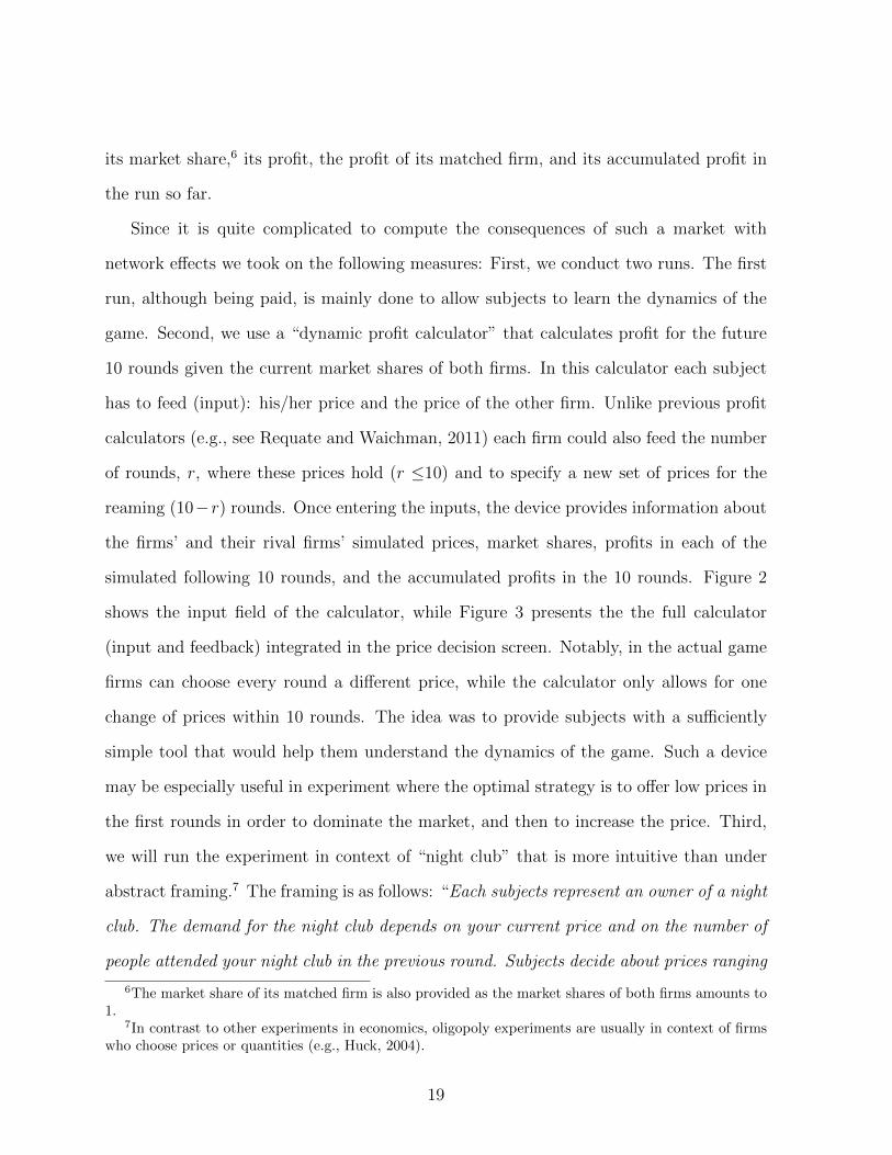
its market share,6 its profit, the profit of its matched firm, and its accumulated profit in
the run so far.
Since it is quite complicated to compute the consequences of such a market with
network e↵ects we took on the following measures: First, we conduct two runs. The first
run, although being paid, is mainly done to allow subjects to learn the dynamics of the
game. Second, we use a “dynamic profit calculator” that calculates profit for the future
10 rounds given the current market shares of both firms. In this calculator each subject
has to feed (input): his/her price and the price of the other firm. Unlike previous profit
calculators (e.g., see Requate and Waichman, 2011) each firm could also feed the number
of rounds, r, where these prices hold (r 10) and to specify a new set of prices for the
reaming (10�r) rounds. Once entering the inputs, the device provides information about
the firms’ and their rival firms’ simulated prices, market shares, profits in each of the
simulated following 10 rounds, and the accumulated profits in the 10 rounds. Figure 2
shows the input field of the calculator, while Figure 3 presents the the full calculator
(input and feedback) integrated in the price decision screen. Notably, in the actual game
firms can choose every round a di↵erent price, while the calculator only allows for one
change of prices within 10 rounds. The idea was to provide subjects with a su�ciently
simple tool that would help them understand the dynamics of the game. Such a device
may be especially useful in experiment where the optimal strategy is to o↵er low prices in
the first rounds in order to dominate the market, and then to increase the price. Third,
we will run the experiment in context of “night club” that is more intuitive than under
abstract framing.7 The framing is as follows: “Each subjects represent an owner of a night
club. The demand for the night club depends on your current price and on the number of
people attended your night club in the previous round. Subjects decide about prices ranging
6The market share of its matched firm is also provided as the market shares of both firms amounts to1.
7In contrast to other experiments in economics, oligopoly experiments are usually in context of firmswho choose prices or quantities (e.g., Huck, 2004).
19

between 0 an 10”
The following figures shows the computer screens. Figure 1 present the location deci-
sion “close” or “far” for the cases it is endogenously determined by the firms. Figure 2
shows the input field of the profit calculator, while Figure 3 shows the decision screen in
a given round.
5 Pre-test results
In September 2013 we conducted some sessions at campus Ribeirao Preto of the Uni-
versity of Sao Paolo, Brazil. We have conducted two treatments with network externality
but when location was either su�ciently close or su�ciently far (these treatments cor-
respond to Treatments 1b and 2b in Table 1). The result we presents in this section
are of the second run of each treatment where subjects are assumed to understood the
environment and the dynamics of the game.
Our preliminary results seems to be quite in line with theory. In the treatment where
firms were located close to each other (e.g. products are roughly homogeneous) the average
price is very low (which corresponds to the subgame perfect equilibrium of the game in
which the market leader choose a price of 5 and the follower choose a price of 0). The
results on average price setting are presented in Figure 4. Moreover, Figure 5 presents
the evolution of markets prices and market shares (demand) of two pairs of firms. In this
cases one can see that once one firm dominated the market, it chose a price of about 5
ECU, where it still have all the market share (because choosing a too high price in relation
with its matched firm may result in loosing market shares). At this point the matched
firms chose minimum price but in vain (the gap between prices of the two firms was not
large enough to attract consumers).
In the treatments where firms are located far from each other (e.g. products are
20

roughly heterogeneous) the average price is about 5 ECU (which corresponds to the
subgame perfect equilibrium of the game in which both players choose a price of 5).
Figure 5 illustrates the evolution of markets prices and market shares (demand) of two
pairs of firms. In these cases since products are di↵erentiated, when the di↵erences in
prices between the firms are not too large there is hardly gain of market shares.
6 Budget
Referencias
Barreda-Tarrazona, I., Garcıa-Gallego, A., Georgantzıs, N., Andaluz-Funcia, J., and Gil-
Sanz, A. (2011). An experiment on spatial competition with endogenous pricing. In-
ternational Journal of Industrial Organization, 29:74–83.
Bayer, R.-C. and Chan, M. (2007). Network externalities, demand inertia and dynamic
pricing in an experimental oligopoly market. Economic Record, 83:405–415.
Becker, G. S. (1991). A note on restaurant pricing and other examples of social influences
on price. Journal of Political Economy, 99:1109–16.
Brown-Kruse, J., Cronshaw, M. B., and Schenk, D. J. (1993). Theory and experiments
on spatial competition. Economic Inquiry, 31:139–65.
Brown Kruse, J. and Schenk, D. J. (2000). Location, cooperation and communication: An
experimental examination. International Journal of Industrial Organization, 18:59–80.
Cabral, L. (2011). Dynamic price competition with network e↵ects. Review of Economic
Studies, 78:83–111.
21

Camacho-Cuena, E., Garcia-Gallego, A., Georgantzis, N., and Sabater-Grande, G. (2005).
Buyer-seller interaction in experimental spatial markets. Regional Science and Urban
Economics, 35:89–108.
Collins, R. and Sherstyuk, K. (2000). Spatial competition with three firms: An experi-
mental study. Economic Inquiry, 38:73–94.
de Almeida Prado, F. P. (2013). Network e↵ects, coalitions of consumers and product
di↵erentiation. Mimeo, University de Sao Paulo.
de Almeida Prado, F. P., Belitsky, V., and Ferreira, A. L. (2011). Social interactions, pro-
duct di↵erentiation and discontinuity of demand. Journal of Mathematical Economics,
47:642–653.
Engel, C. (2007). How much collusion? a meta-analysis of oligopoly experiments. Journal
of Competition Law and Economics, 3:491–549.
Fischbacher, U. (2007). z-Tree: Zurich toolbox for ready-made economic experiments.
Experimental Economics, 10:171–178.
Fonseca, M. A. and Normann, H.-T. (2012). Explicit vs. tacit collusionthe impact of
communication in oligopoly experiments. European Economic Review, 56:1759–1772.
Fouraker, L. E. and Siegel, S. (1963). Bargaining Behavior. McGrawHill, New York.
Hoggatt, A. C. (1959). An experimental business game. Behavioral Science, 4:192–203.
Huck, S. (2004). Oligopoly. In Friedman, D. and Cassar, A., editors, Economics Lab: An
Intensive Course in Experimental Economics, pages 105–114. Routledge, London.
Huck, S., Muller, W., and Vriend, N. J. (2002). The east end, the west end, and king’s
cross: on clustering in the four-player hotelling game. Economic Inquiry, 40:231–240.
22

Keser, C. (1993). Some results of experimental duopoly markets with demand intertia.
Journal of Industrial Economics, 41:133–51.
Keser, C. (2000). Cooperation in symmetric duopolies with demand inertia. International
Journal of Industrial Organization, 18:23–38.
Mitchell, M. and Skrzypacz, A. (2006). Network externalities and long-run market shares.
Economic Theory, 29:621–648.
Orzen, H. and Sefton, M. (2008). An experiment on spatial price competition. Internati-
onal Journal of Industrial Organization, 26:716–729.
Potters, J. and Suetens, S. (2013). Oligopoly experiments in the current millennium.
Journal of Economic Surveys, 27:439–460.
Requate, T. and Waichman, I. (2011). a profit table or a profit calculator? a note on the
design of cournot oligopoly experiments. Experimental Economics, 14:36–46.
Sauermann, H. and Selten, R. (1959). Ein oligopolexperimen. Zeitschrift fur die gesamte
Staatswissenschaft (JITE), 115:427471.
Selten, R. (1965). Spieltheoretische behandlung eines oligopolmodells mit nachfra-
getragheit. Zeitschrift fur die gesamte Staatswissenschaft (JITE), 121:301–324.
Waichman, I., Reqaute, T., and Siang, C. K. (2014). Communication in cournot compe-
tition: An experimental study. Mimeo, University of Kiel.
23

The first stage in treatments where it is displayed. Subjects choose whether to be located close to or farfrom the other firm
Figura 1: The location-decision screen.
In this example a subjects calculates the profits under the following condition in the first 6 rounds hisprice is 1 the other firm price is 5. The the remaining 4 rounds he increases his price to 10, while theother firm price is 5.
Figura 2: The input of the profit calculator
24

The profit calculator is located on the left-hand side of the screen. The results of the previous roundare shown on the upper right-hand side of the screen, while the price decision is made on the bottomright-hand side. Given the input inserted to the profit calculator (see Figure 2) the calculator indicatethat the firm will have the whole market share already in the next second round. which lead to a profitof 45.90 ECU after 10 rounds. The history of actual play indicate that both firms chose a price of 5 inthe previous round and share the market equally (each receiving a profit of 2.5 ECU so far).
Figura 3: The price-decision screen (round 2 of 20).
25

1 2 3 4 5 6 7 8 9 10 11 12 13 14 15 16 17 18 19 200
1
2
3
4
5
6
7
8
9
10
Periods
Price
Group close20
1st and 3rd quartilesMedian
(a) Firms are located close to each other
1 2 3 4 5 6 7 8 9 10 11 12 13 14 15 16 17 18 19 200
1
2
3
4
5
6
7
8
9
10
Periods
Price
Group Far
1st and 3rd quartilesMedian
(b) Firms are located far from each other
Figura 4: Median prices across di↵erent markets in Treatments 1b (above) and 2b (below).
26

1 2 3 4 5 6 7 8 9 10 11 12 13 14 15 16 17 18 19 200
1
2
3
4
5
6
7
8
9
10
Price
1 2 3 4 5 6 7 8 9 10 11 12 13 14 15 16 17 18 19 200
0.1
0.2
0.3
0.4
0.5
0.6
0.7
0.8
0.9
1
Dem
and
(a) Pair 1
1 2 3 4 5 6 7 8 9 10 11 12 13 14 15 16 17 18 19 200
1
2
3
4
5
6
7
8
9
10
Price
1 2 3 4 5 6 7 8 9 10 11 12 13 14 15 16 17 18 19 200
0.1
0.2
0.3
0.4
0.5
0.6
0.7
0.8
0.9
1
Dem
and
(b) Pair 2
Figura 5: Dynamics of price and market shares (demands) of two pairs of firms locatedclose to each other (Treatment 1b)
27

1 2 3 4 5 6 7 8 9 10 11 12 13 14 15 16 17 18 19 200
1
2
3
4
5
6
7
8
9
10
Price
1 2 3 4 5 6 7 8 9 10 11 12 13 14 15 16 17 18 19 200
0.1
0.2
0.3
0.4
0.5
0.6
0.7
0.8
0.9
1
Dem
and
(a) Pair 1
1 2 3 4 5 6 7 8 9 10 11 12 13 14 15 16 17 18 19 200
1
2
3
4
5
6
7
8
9
10
Price
1 2 3 4 5 6 7 8 9 10 11 12 13 14 15 16 17 18 19 200
0.1
0.2
0.3
0.4
0.5
0.6
0.7
0.8
0.9
1
Dem
and
(b) Pair 2
Figura 6: Dynamics of price and market shares (demands) of two pairs of firms locatedfar to each other (Treatment 2b)
28