research article one-step-ahead predictive control for

Research ArticleOne-Step-Ahead Predictive Control for Hydroturbine Governor

Zhihuai Xiao,1 Suili Meng,1 Na Lu,2 and O. P. Malik3

1School of Power and Mechanical Engineering, Wuhan University, Wuhan, Hubei 430072, China2School of Water Resources and Architectural Engineering, Northwest A&F University, Xi’an, Shaanxi 712100, China3Department of Electrical and Computer Engineering, University of Calgary, Calgary, AB, Canada T2N 1N4

Correspondence should be addressed to Zhihuai Xiao; [email protected]

Received 24 December 2014; Accepted 23 January 2015

Academic Editor: Yun-Bo Zhao

Copyright © 2015 Zhihuai Xiao et al. This is an open access article distributed under the Creative Commons Attribution License,which permits unrestricted use, distribution, and reproduction in any medium, provided the original work is properly cited.

The hydroturbine generator regulating system can be considered as one system synthetically integrating water, machine, andelectricity. It is a complex and nonlinear system, and its configuration and parameters are time-dependent. A one-step-aheadpredictive control based on on-line trained neural networks (NNs) for hydroturbine governor with variation in gate positionis described in this paper. The proposed control algorithm consists of a one-step-ahead neuropredictor that tracks the dynamiccharacteristics of the plant and predicts its output and a neurocontroller to generate the optimal control signal. The weights of twoNNs, initially trained off-line, are updated on-line according to the scalar error. The proposed controller can thus track operatingconditions in real-time and produce the optimal control signal over the wide operating range. Only the inputs and outputs of thegenerator are measured and there is no need to determine the other states of the generator. Simulations have been performed withvarying operating conditions and different disturbances to compare the performance of the proposed controller with that of aconventional PID controller and validate the feasibility of the proposed approach.

1. Introduction

Hydroturbine governor (HTG) provides the basic controlin hydropower stations to ensure the reliability and thequality of electricity supply. The conventional hydroturbinegovernor adopted by most utilities is a proportional, integral,and derivative (PID) type controller based on linear controltheory. It has simple structure with flexibility and is easy forimplementation, and thus it has made a great contribution inenhancing the quality of electrical supply [1].

The hydroturbine generator regulating system can beconsidered as one system synthetically integrating water,machine, and electricity. It is a complex andnonlinear system,and its configuration and parameters are time-dependent[2]. Nonlinear models are required when speed and powerchanges are large during an islanding, load rejection, andsystem restoration conditions. A nonlinear model shouldinclude the effect of water compressibility, that is, inclusion oftransmission-line-like reflections which occur in the elastic-walled pipe carrying compressible fluid [3, 4].

This creates discrepancies between the mathematicallinear model of the hydroturbine generator regulating sys-tem and the physical nonlinear plant. Therefore, with theconventional linear control theory based PID controller, itis difficult to realize the desired control performance overwide operating conditions of the power plant [5]. To yieldsatisfactory control performance, it is desirable to develop acontroller that considers the nonlinear nature of the plant andhas the ability to adjust its parameters on-line according to theenvironment in which it is working, that is, track the plantoperating conditions [6].

To meet this requirement, a large amount of researchhas been conducted on the hydroturbine generator regulat-ing system. Numerous methods for PID tuning have beenreported in the literature [7]. For example, to realize theparameter optimization of PID controller, an orthogonaltest strategy is adopted in [8, 9] for hydroturbine controlapplication. In this approach, a control performance indexthat depends on control parameters KP, Ki, and Kd is defined.Each of these parameters is considered under various levels as

Hindawi Publishing CorporationMathematical Problems in EngineeringVolume 2015, Article ID 382954, 10 pageshttp://dx.doi.org/10.1155/2015/382954

2 Mathematical Problems in Engineering

a discrete variable. An optimization algorithm is developedto search for better control parameters in the neighbouringspace of the present one. However, many of these approacheslack one or more of the three basic and important featuresthat a controller should have, that is, simplicity of structure,fast acting (low computation time), and adaptability.

Neural networks (NNs) have been applied very success-fully in the identification and control of dynamic systems.Theuniversal approximation capabilities of themultilayer percep-tronmake it a popular choice formodeling nonlinear systemsand implementing general-purpose nonlinear controllers[10–13]. The concept of intelligent tuning of PID controlleris presented in [14, 15]. The use of adaptive learning controlschemes is discussed in [14] and the improved dynamic per-formance of the intelligent PID controller over the conven-tional PID is presented in [15]. The developed intelligent PIDcontroller is based on anthropomorphic intelligence. Amongvarious types of NNs used in the hydroturbine generator reg-ulating system, the feed-forward multilayer NN is the mostcommonly used. This is mainly due to the computationalefficiency of the back propagation algorithm [12] and the ver-satility of the three-layer feed-forward NN in approximatingan arbitrary static nonlinear function [16]. However, littlework has been reported on the use of NNs for hydroturbinegenerator regulating system for real-time control.

The theory and algorithm of predictive control haveachieved great development in the industrial process controlafter thirty years’ application and study. It has been intro-duced to the optimal control of hydroturbines by lots ofexperts. Jones andMansoor [17], for example, applied predic-tive feed-forward control to the power target signal trackingin part load condition, and the result shows that predictivefeed-forward control can achieve a substantial improvementin tracking a power target when a hydroelectric station oper-ates in part load conditionmode. However, the power stationthey used is modeled using linearized transfer function. Forsystems with strong nonlinear and frequent turbulence orwide range of operating point, the predictive control adoptinglinear model near operating point can no longer satisfy therequirements of control quality. Therefore, the nonlinearmodeled predictive control has aroused wide concern.

A predictive control scheme for hydroturbine governorbased on NNs is introduced in this paper. The controlarchitecture consists of two NNs: an adaptive neuroidentifier(ANI) to track the plant and predict its output one-step-aheadand an adaptive neurocontroller (ANC) to produce the con-trol signal. A scalar error is used in each sampling period toupdate the identifier and controller weights continuously inreal-time.With a similar architecture, called indirect adaptivecontrol [12], the use of a reference model is suggested. Thatis avoided in this work owing to the difficulties in choosinga proper reference model for the complex hydroturbinegenerator regulating system.

The effect of different amplitude step disturbances andtrapezoidal shape reference signal (turbine power) are inves-tigated in this paper. Also, a number of studies are performedto compare the performance of the proposed controllerwith that of the conventional PID controller under differentoperating conditions.

2. Basic Plant Equations

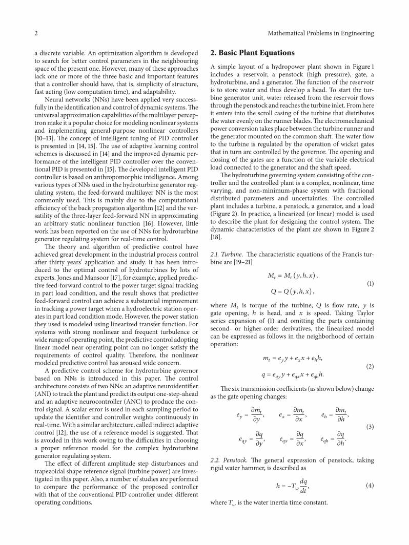
A simple layout of a hydropower plant shown in Figure 1includes a reservoir, a penstock (high pressure), gate, ahydroturbine, and a generator. The function of the reservoiris to store water and thus develop a head. To start the tur-bine generator unit, water released from the reservoir flowsthrough the penstock and reaches the turbine inlet. Fromhereit enters into the scroll casing of the turbine that distributesthe water evenly on the runner blades.The electromechanicalpower conversion takes place between the turbine runner andthe generator mounted on the common shaft.The water flowto the turbine is regulated by the operation of wicket gatesthat in turn are controlled by the governor. The opening andclosing of the gates are a function of the variable electricalload connected to the generator and the shaft speed.

Thehydroturbine governing system consisting of the con-troller and the controlled plant is a complex, nonlinear, timevarying, and non-minimum-phase system with fractionaldistributed parameters and uncertainties. The controlledplant includes a turbine, a penstock, a generator, and a load(Figure 2). In practice, a linearized (or linear) model is usedto describe the plant for designing the control system. Thedynamic characteristics of the plant are shown in Figure 2[18].

2.1. Turbine. The characteristic equations of the Francis tur-bine are [19–21]

𝑀𝑡= 𝑀𝑡(𝑦, ℎ, 𝑥) ,

𝑄 = 𝑄 (𝑦, ℎ, 𝑥) ,

(1)

where 𝑀𝑡is torque of the turbine, 𝑄 is flow rate, 𝑦 is

gate opening, ℎ is head, and 𝑥 is speed. Taking Taylorseries expansion of (1) and omitting the parts containingsecond- or higher-order derivatives, the linearized modelcan be expressed as follows in the neighborhood of certainoperation:

𝑚𝑡= 𝑒𝑦𝑦 + 𝑒𝑥𝑥 + 𝑒ℎℎ,

𝑞 = 𝑒𝑞𝑦𝑦 + 𝑒𝑞𝑥𝑥 + 𝑒𝑞ℎℎ.

(2)

The six transmission coefficients (as shownbelow) changeas the gate opening changes:

𝑒𝑦=𝜕𝑚𝑡

𝜕𝑦, 𝑒

𝑥=𝜕𝑚𝑡

𝜕𝑥, 𝑒

ℎ=𝜕𝑚𝑡

𝜕ℎ,

𝑒𝑞𝑦=𝜕𝑞

𝜕𝑦, 𝑒

𝑞𝑥=𝜕𝑞

𝜕𝑥, 𝑒

𝑞ℎ=𝜕𝑞

𝜕ℎ.

(3)

2.2. Penstock. The general expression of penstock, takingrigid water hammer, is described as

ℎ = −𝑇𝑤

𝑑𝑞

𝑑𝑡, (4)

where 𝑇𝑤is the water inertia time constant.

Mathematical Problems in Engineering 3

ReservoirPenstock

Gate

Hydroturbine

Draft tube

Generator

Figure 1: General layout of hydropower plant.

Servomechanism

Penstock system

Turbine

Load

Generatoryu

q h

xMt−

+

Mg

Figure 2: Hydroturbine generator regulating system.

2.3. Generator and Load. The characteristic equation of thegenerator and the load can be written as

𝑇𝑎

𝑑𝑥

𝑑𝑡= 𝑚𝑡− 𝑚𝑔− 𝑒𝑔𝑥, (5)

where 𝑇𝑎is the unit inertia time constant, 𝑚

𝑔is the load

torque, and 𝑒𝑔is the load self-regulation factor, regarding the

fluctuation caused by the change of the system frequency.

2.4. Servomechanism. Neglecting small time constants, theservomechanism can be expressed with a first-order equa-tion:

𝑇𝑦

𝑑𝑦

𝑑𝑡+ 𝑦 = 𝑢, (6)

where𝑇𝑦is the servomotor response time and 𝑢 is the control

signal.

3. Controller Structure

The structure of the controller is shown in Figure 3. It consistsof two subnetworks. The first subnetwork is an adaptive one-step-ahead neuroidentifier that tracks the dynamic behaviourof the plant and identifies the plant in terms of its internalweights and the second one is an adaptive neurocontrollerto provide the necessary control action in order to minimizecertain cost function.

3.1. Adaptive Neuroidentifier. Amultilayer perceptron neuralnetwork (MLPNN) structure is developed to model thenonlinear dynamic relationship between the gate positionand the turbine mechanical power. Considering it is difficultto measure the turbine mechanical power, generator output

power is measured instead to obtain the turbine mechanicalpower by

𝑃𝑒=

𝑃𝑔

𝜂, (7)

where 𝑃𝑒is turbine mechanical power, 𝑃

𝑔is generator output

power, and 𝜂 is generator efficiency.The network transforms 𝑛 inputs to 𝑚 outputs through a

nonlinear function 𝑓 : 𝑅𝑛 → 𝑅𝑚. It is shown in [15] that an

MLPNN with single hidden layer activated with sigmoid orhyperbolic tangent function can approximate any continuousfunction. Considering the nature of the dependence of theplant output on a finite number of past inputs, 𝑢(𝑡), andoutputs, 𝑦(𝑡), the nonlinear relationship between the gateposition and the turbine power can be represented in the formof predictor/identifier as

𝑦(𝑘+1)

= 𝑓 [𝑦(𝑘), 𝑦(𝑘−1)

, . . . , 𝑦(𝑘−𝑛+1)

, 𝑢(𝑘), 𝑢(𝑘−1)

, . . . , 𝑢(𝑘−𝑚+1)

] .

(8)

In this case a popular MLPNN with single hidden layeractivated with sigmoid function and back propagation learn-ing has been used to develop the predictor of nonlinearrelationship model (8). The input vector to the ANI is

[𝑝(𝑘), 𝑝(𝑘−1)

, . . . , 𝑝(𝑘−𝑛+1)

,

𝑢(𝑘), 𝑢(𝑘−1)

, . . . , 𝑢(𝑘−𝑚+1)

] ,

(9)

where 𝑝(𝑘) is the turbine mechanical power and 𝑢(𝑘) isthe gate position at the time step 𝑘. The output is thepredicted turbinemechanical power𝑝

(𝑘+1), at time step (𝑘+1).

For a finite number of past inputs, 𝑢(𝑡), and outputs, 𝑝(𝑡),the nonlinear relationship between the control output (gateposition) and turbine power can be represented in the formof an identifier as shown in Figure 4.

The input vector to the ANI is scaled in the rangeof [−1, +1] before being applied to the network. The costfunction used for the ANI is

𝐽𝑖(𝑘) =

1

2𝑒𝑖(𝑘)2=1

2[𝑝 (𝑘) − 𝑝(𝑘)]

2

. (10)

The weights are updated as

𝑤𝑖(𝑘) = 𝑤

𝑖(𝑘 − 1) − 𝜂

𝑖

𝜕𝐽𝑖(𝑘)

𝜕𝑤𝑖(𝑘), (11)

where 𝑤𝑖is the matrix of identifier weights at time step 𝑘

and 𝜂𝑖is the learning rate for the ANI. This cost function

is minimized by back propagating the scalar error. In eachsampling period, the input and the output of the plant aresampled and the input vector to the identifier is formed as in(9). Then the error between the actual and predicted outputsof the plant, a scalar value, is back propagated through theidentifier to update the weights of the network (𝑤

𝑖(𝑘)). This

process is repeated every sampling period that in turn resultsin an adaptive approach to predict one-step-ahead of theoutput of the plant. The use of just one error value for backpropagation simplifies the training algorithm by reducingcomputation time.


Plant

Neuroidentifier

D

D

D

D

D

D

Reference signalPe

Pe

−

+

u

ep

ec

−

+

Neuroidentifier

Figure 3: Schematic of control structure.

Feed-forward multilayer

neural network

p(k)

p(k−n)

u(k)

u(k−m)

p(k+1)

...

...

Figure 4: Neuroidentifier.

3.2. Adaptive Neurocontroller. Taking advantage of the recog-nized universal approximation properties of NN, a nonlinearplant in the MLPNN form is obtained as discussed before.Based on the neural model, a predictive control strategyis implemented by an adaptive neurocontroller. The inputvector to the ANC is

[𝑝(𝑘), 𝑝(𝑘−1)

, . . . , 𝑝(𝑘−𝑝+1)

,

𝑟(𝑘), 𝑟(𝑘−1)

, . . . , 𝑟(𝑘−𝑞+1)

] ,

(12)

where 𝑟(𝑘) is the reference input signal at time step 𝑘. Theoutput of the ANC is the control action 𝑢(𝑘) at time step 𝑘.The inputs to the ANC are also scaled in the range of [−𝑙, +𝑙].The cost function for the ANC is considered as

𝐽𝑐(𝑘) =

1

2[𝑒𝑐(𝑘)2+ ℎ𝑢 (𝑘)]

2

=1

2[𝑟 (𝑘) − 𝑝(𝑘)]

2

+ℎ

2𝑢 (𝑘)2,

(13)

where 𝑟(𝑘) is the reference input signal at time step 𝑘 andℎ is a tuning parameter that is used to improve the plantoutput dynamic characteristics. By taking ℎ larger than zero,a penalty factor is applied to the control operation that helpsthe tuning of the dynamic trajectory and optimizing theovershoot and the settling time of the response curve. Theweights of the controller 𝑤

𝑐(𝑘) are updated as

𝑤𝑐(𝑘) = 𝑤

𝑐(𝑘 − 1) − 𝜂

𝑐

𝜕𝐽𝑐(𝑘)

𝜕𝑤𝑐(𝑘). (14)

Using (13) and (14) 𝐽𝑐(𝑘) is minimized in each sampling

period. As depicted in (9) and (12), the states of the plant arenot required for the implementation of the ANI and ANC,and only input-output data are needed.This greatly simplifiesthe implementation of the control process.

4. Training Process

The success implementation of the control algorithm pre-sented in Section 3 highly depends on the accuracy of theidentifier in tracking dynamic plant. For this reason, theANI is initially trained off-line before being used in the finalconfiguration.The training is performed over a wide range ofoperating conditions for the generating unit. After the off-linetraining stage, the ANI is employed in the system. Furtherupdating of the weights of ANI and ANC is performed ineach sampling period by employing the on-line version ofthe back propagation method. This enables the controller totrack the plant variations as they occur to yield the optimumperformance. The main steps of the adaptive predictivecontrol algorithm are listed as follows, and the algorithmflowchart is shown in Figure 5.

(1) At time step 𝑘, 𝑝(𝑘) is sampled.(2) Compute 𝑝

(𝑘)using ANI and its input vector (9).

(3) Calculate the error between 𝑝(𝑘) and 𝑝(𝑘); then

update the weights of the ANI to minimize 𝐽𝑖(𝑘) uti-

lizing the back propagation method and the gradientdescent algorithm.

(4) The output of the controller 𝑢(𝑘) is computed.(5) Using input vector (9), the predicted 𝑝

(𝑘+1)is com-

puted by the ANI with weights updated in step (3).(6) Based on 𝑝

(𝑘+1)and reference signal, weights of the

ANC are updated, minimizing 𝐽𝑐(𝑘) by utilizing the

back propagation method and the gradient descentalgorithm.

In step (3) above, the training is straightforward sincethe error at the output of the ANI is obtained. However, in


Update the weights of ANI

Update the weights of ANC

Sample p(k)

p(k) = f[p(k−1), p(k−2), . . . , p(k−n), u(k−1), u(k−2), . . . , u(k−m)], by ANI

p(k+1) = f[p(k), p(k−1), . . . , p(k−n+1), u(k), u(k−1), . . . , u(k−m+1)], by ANI

u(k) = f([p(k), p(k−1), . . . , p(k−p+1), r(k), r(k−1), . . . , r(k−q+1)]), by ANC

Ji(k) =1

2[p(k) − p(k)]

2

Jc(k) =1

2[r(k) − p(k)]

2+h

2u(k)2

Figure 5:Theflowchart of the adaptive predictive control algorithm.

step (6) the training is difficult since the error at the outputof the ANC is not provided. In this case, first, the weightsof the ANI are frozen and the error between the desired andpredicted plant output is back propagated through the ANI.Then, the back propagated signal at the input of the ANIis further propagated through the ANC, making necessarychanges to the controllerweights. In otherwords, for adaptingweights of the controller, the identifier acts as a channel toconvey the error from the output of the identifier to the outputof the controller.This evaluates the need to have the identifier.The error is used to train the ANI and the ANC.

5. Simulation Results

The plant model is simulated using the mathematical modelgiven in Section 2. The values of plant parameters used are

𝑇𝑎= 9.06 s, 𝑇

𝑤= 1.27 s, 𝑇

𝑟= 0.15 s,

𝜉 = 0.2, 𝑇1= 0.02 s, 𝑇 = 0.04 s,

𝑠1= 0.00167, 𝑖

𝑥= 0.04%,

(15)

where 𝑇𝑟is penstock reflection time, 𝜉 is damping constant-

infinite bus tie, 𝑇1is servomotor response time, 𝑇 is the

sampling period, 𝑠1is speed limit on control in a governor,

and 𝑖𝑥is dead band. The transmission coefficients (except

𝑒𝑞𝑥

which is usually equal to 0) have different values for thedifferent gate openings. A set of transmission coefficientscorresponding to the gate opening for a turbine located inOuyanghai hydropower plant in China is given in Table 1.Thedesign water head of Ouyanghai hydropower station is 37.6meters, and design flow is 38.4m3/s. Turbinemodel is chosenasHL123-LJ-225, and rated capacity and voltage of the turbineare 1200 kw and 10.5 kv, respectively.

Table 1: Transmission coefficients as a function of gate opening.

Operatingpointnumber

Gateopening % 𝑒

𝑦𝑒ℎ

𝑒𝑥

𝑒𝑞𝑦

𝑒𝑞ℎ

1 43.74 2.867 0.526 −0.353 1.674 0.2322 47.52 2.562 0.679 −0.455 1.541 0.2623 51.26 2.278 0.814 −0.545 1.416 0.2904 55 2.016 0.934 −0.626 1.300 0.3155 58.74 1.766 1.039 −0.696 1.191 0.3386 62.52 1.654 1.132 −0.759 1.090 0.3607 66.26 1.333 1.212 −0.813 0.997 0.3808 70 1.146 1.281 −0.859 0.913 0.3979 73.74 0.974 1.340 −0.898 0.837 0.41410 77.52 0.822 1.391 −0.932 0.768 0.42911 81.26 0.691 1.433 −0.961 0.708 0.44312 85 0.578 1.468 −0.984 0.655 0.45513 88.74 0.484 1.498 −1.000 0.611 0.46714 92.52 0.409 1.523 −1.020 0.574 0.47815 96.26 0.353 1.544 −1.030 0.546 0.48916 100 0.317 1.563 −1.047 0.526 0.499

The Simulation Toolbox SIMULINK of MATLAB is uti-lized to develop plant model and generate data. The absolutevalue of pseudorandombinary signal is applied to the input torepresent the variation of gate position, and the correspond-ing turbine mechanical power is obtained. The data collected(input and output) are divided into two sets: one set is fortraining the NN and the other set is for validation.

An input-output identifier model and control strategy isestablished and its parameters are set as follows. The numberof time delays used for the input of ANI and ANC is set to 3;that is,𝑚, 𝑛, 𝑝, and 𝑞 in (8), (9), and (12) are all set to 3. Thismeans that both the ANI and the ANC have 6 inputs. Thereis one hidden layer of 8 neurons with sigmoid nonlinearityand an output layer with one linear neuron, for both the ANIand the ANC. Initial weights of the ANC lie in [−0.1, +0.1],chosen randomly at the beginning of the process. The initialweights of the ANI are set to those obtained from off-linetraining stage of the ANI as discussed before. The learningrate for the ANI and the ANC is 0.01 and 0.03, respectively.The value of the penalty factor ℎ is set between 0.1 and 2.0.

The quadratic programming problem in (13) is solved byusing the quadprog function in the Optimization Toolbox ofMATLAB. The MLP network algorithm is realized by usingthe functions of Train, Init, and Sim in the Neural NetworkToolbox of MATLAB.

As the control parameters have been determined asdiscussed before, the performance of the proposed adaptiveneural predictive control is simulated on a large amplitudestep and trapezoidal wave-shape reference signals. Thesereference signals may represent the nature of load changes.The turbine gate opening and power output are shown inFigures 6–9 on different reference signals and various valuesof penalty factor ℎ.


0 10 20 30 40 50 60 70 80 90 1000

0.2

0.4

0.6

0.8

1

1.2

Time (s)

Turb

ine p

ower

(pu)

ReferenceOutput

(a) Turbine power output response

0 10 20 30 40 50 60 70 80 90 1000

0.2

0.4

0.6

0.8

1

Time (s)

Gat

e pos

ition

(b) Turbine gate opening response

Figure 6: Response to large amplitude step in turbine power reference, ℎ = 2.0.

0 20 40 60 80 1000

0.2

0.4

0.6

0.8

1

1.2

1.4

Time (s)

Turb

ine p

ower

(pu)

ReferenceOutput


0 10 20 30 40 50 60 70 80 90 1000

0.2

0.4

0.6

0.8

1

Time (s)

Gat

e pos

ition


Figure 7: Response to large amplitude step in turbine power reference, ℎ = 0.18.

The response shows a non-minimum-phase characteris-tic. The turbine power response on the large amplitude stepsignal follows more or less closely. It is evident that despitea large change in the operating conditions the controllerstill provides good results because of the adaptation process.However, the gate position is observed to exhibit largefluctuation on step change with ℎ = 0.18. This wouldcause undue actuator wear. The optimization seems to beinsensitive to variations in control penalty factor. In the case

of trapezoidal wave signal, the controlled variable reachesits steady-state value extremely fast with a little offset (i.e.,output power overlaps the reference signal) and gate positionvariation within limits is demonstrated.

A number of studies have been performed to compare thequality of the proposed adaptive predictive controller withthose of the conventional PID controller.

Generally, the conventional governors adopt a PI or PIDcontrol law. Figure 10 is the illustration of the conventional


0 20 40 60 80 1000

0.2

0.4

0.6

0.8

1

Time (s)

Turb

ine p

ower

(pu)

ReferenceOutput


0 20 40 60 80 1000

0.2

0.4

0.6

0.8

1

Time (s)

Gat

e pos

ition


Figure 8: Response to trapezoidal wave reference, ℎ = 2.0.

0 20 40 60 80 1000

0.2

1.2

0.4

0.6

0.8

1

Time (s)

Turb

ine p

ower

(pu)

ReferenceOutput


0 20 40 60 80 1000

0.2

0.4

0.6

0.8

1

Time (s)

Gat

e pos

ition


Figure 9: Response to trapezoidal wave reference, ℎ = 0.18.

Turbinepenstock

and generatorServomotor

P

I

D

Load reference

Speed reference

Speed

Power

++

+

+

+

−

−

−

bp

Figure 10: Illustration of the conventional load-change method.


load changing process, where bp is permanent speed droop.It plays an important role in adjusting the load of the unit andthe load distribution among all units in the power system.

Regarding the adjustments of PID parameters, the follow-ing formulas are often used by experienced engineers.

For PI controller,

𝑇𝑛= 0, 𝑏

𝑡=2.6𝑇𝑤

𝑇𝑎

, 𝑇𝑑= 6𝑇𝑤; (16)

for PID controller,

𝑇𝑛= 0.5𝑇

𝑤, 𝑏

𝑡=1.5𝑇𝑤

𝑇𝑎

, 𝑇𝑑= 3𝑇𝑤, (17)

where 𝑇𝑛is the derivative time constant, 𝑏

𝑡is the transient

speed droop, and 𝑇𝑑is the damping time constant. Their

relation with proportional, integral, and differential gaincoefficients of a continuous PID controller is

𝑘𝑝=𝑇𝑑+ 𝑇𝑛

𝑏𝑡𝑇𝑑

, 𝑘𝑖=

1

𝑏𝑡𝑇𝑑

, 𝑘𝑑=𝑇𝑛

𝑏𝑡

. (18)

According to these empirical formulae, the parameters ofthe conventional PID controller are chosen as below:

𝑘𝑝= 5.56, 𝑘

𝑖= 1.25, 𝑘

𝑑= 3.03, 𝑏

𝑝= 0.

(19)

The proposed adaptive neuropredictive controller adoptsthe parameters determined as discussed above and the valueof the penalty factor ℎ is set to 2.0.

Step increases of 10% and 80% in power reference areintroduced and the system responses with the conventionalPID controller (CPID) and the proposed adaptive neuropre-dictive controller (PAPC) are shown in Figures 11–14. Thedashed curves represent the response of CPID, and the solidlines represent the response of PAPC.

It is observed from Figure 11 that, with the conventionalPID controller, the settling time, defined as themomentwhenthe system error is less than 5% of the input reference signal,is 8.9 s and the overshoot is 18.3%, but, with the adaptivepredictive controller, the setting time is 7.2 s and overshoot is13.1%. It can be seen from Figure 12 that the settling time withthe conventional PID controller is 28.3 s and the overshoot is37.4%, but, with the adaptive predictive controller, the settingtime is 7.4 s and overshoot is 13.5%.

From the responses for 10% and 80% step changesin power reference, it can be seen that the conventionalPID controller only provides acceptable performance for asmall disturbance rather than the large disturbance. Evenfor a small disturbance, the proposed adaptive predictivecontroller is better than the conventional one regarding thespeed and the overshoot of response of the process.

This is logically correct because of the existence ofnonlinearities in a hydroturbine governing system. Thesenonlinearities can be divided into two parts. The first comesfrom the turbine’s nonlinear characteristics that depend onthe operating point. It can be clearly seen from (2) ofthe turbine that the six transmission coefficients change

CPIDPAPC

0 10 20 30 40 500

0.02

0.04

0.06

0.08

0.1

0.12

0.14

Time (s)

Turb

ine p

ower

(pu)

Figure 11: Turbine power output response to a 10% step in reference.

CPIDPAPC

0 10 20 30 40 500

0.2

0.4

0.6

0.8

1

1.2

Time (s)

Turb

ine p

ower

(pu)

Figure 12: Turbine power output response to an 80% step in refer-ence.

as the gate opening changes. The second part is due tothe nonlinear factors such as magnitude limit on control,dead band, and speed limit on control. Therefore, in theconventional PID controller, the regulation parameters thatgive good performance for small disturbance are no longeroptimal for the large disturbance. In the case of a smalldisturbance, the effect of nonlinearity is negligible and theconventional controller is designed based on the linearcontrol theory, but, in the case of a large disturbance, theeffect of nonlinearity cannot be neglected. The plant haschanged; however the control parameters of the conventionalPID controller have not changed. Therefore, it is unable tomaintain adequate performance levels. In contrast, it can be


CPIDPAPC

0 10 20 30 40 500

0.02

0.04

0.06

0.08

0.1

0.12

0.14

Time (s)

Turb

ine p

ower

(pu)

Figure 13: Gate opening response to a 10% step in reference.

CPIDPAPC

0 10 20 30 40 500

0.2

0.4

0.6

0.8

1

1.2

Time (s)

Turb

ine p

ower

(pu)

Figure 14: Gate opening response to an 80% step in reference.

seen that the proposed adaptive predictive controller has agood response for both small and large disturbances, becauseit considers the nonlinear nature of the plant and has theability to adjust its own parameters on-line according tothe working environment. Even for the small disturbance,the proposed adaptive predictive controller considers theplant nonlinearity as well, while it is usually ignored inthe conventional PID controller. Therefore, the proposedadaptive predictive controller has better control performancethan the conventional one in regard to the speed and theovershoot of the process response.

6. Conclusions

An adaptive neuropredictive control for hydroturbine gov-ernor is presented in this paper. The back propagation net-work with on-line learning is used in the proposed method.The controller introduced in this work inherits the generaladvantages of neural networks such as high speed, general-ization capability, and fault tolerance as well as adaptation(learning) property. This method features the simple struc-ture and the nonrequirement for a large number of neuronsin the implementation. The learning algorithm is simplifiedby employing a single element error vector. The controllerweights are updated directly in an on-line mode from theinputs and the outputs of the generator, and the statesof the system are not necessarily determined. Simulationresults for the large amplitude step and trapezoidal wave-shape reference signals show that the proposed adaptivepredictive controller can adaptively improve the dynamicperformance of the system. By comparing the performanceof the proposed adaptive predictive controller with that ofthe conventional PID controller, it is found that the proposedadaptive predictive controller is not only simple but alsorobust, and it features strong adaptivity as well.

Conflict of Interests

The authors declare that there is no conflict of interestsregarding the publication of this paper.

Acknowledgment

The authors acknowledge the financial supports from theNational Natural Science Foundation of China under Grantno. 51379160.

References

[1] N. Kishor, R. P. Saini, and S. P. Singh, “A review on hydropowerplant models and control,” Renewable and Sustainable EnergyReviews, vol. 11, no. 5, pp. 776–796, 2007.

[2] H. Fang, L. Chen, and Z. Shen, “Application of an improvedPSO algorithm to optimal tuning of PID gains for water turbinegovernor,” Energy Conversion and Management, vol. 52, no. 4,pp. 1763–1770, 2011.

[3] D. G. Ramey and J. W. Skooglund, “Detailed hydro governorrepresentation for system stability studies,” IEEE Transactionson Power Apparatus and Systems, vol. 89, no. 1, pp. 106–112, 1970.

[4] Q. Chen and Z. Xiao, “Dynamic modeling of hydroturbine gen-erating set,” in Proceedings of the IEEE International Conferenceon Systems,Man and Cybernetics, pp. 3427–3430, October 2000.

[5] C. Jiang, Y. Ma, and C. Wang, “PID controller parameters opti-mization of hydro-turbine governing systems using determin-istic-chaotic-mutation evolutionary programming (DCMEP),”Energy Conversion and Management, vol. 47, no. 9-10, pp. 1222–1230, 2006.

[6] D. Zhang and L. Yu, “Exponential state estimation for Marko-vian jumping neural networks with time-varying discrete anddistributed delays,” Neural Networks, vol. 35, pp. 103–111, 2012.


[7] P. Husek, “PID controller design for hydraulic turbine basedon sensitivity margin specifications,” International Journal ofElectrical Power and Energy Systems, vol. 55, pp. 460–466, 2014.

[8] Z. Li and O. P. Malik, “An orthogonal test approach basedcontrol parameter optimization and its application to a hydro-turbine governor,” IEEE Transactions on Energy Conversion, vol.12, no. 4, pp. 388–393, 1997.

[9] A. Soos and O. P. Malik, “An H2optimal adaptive power system

stabilizer,” IEEE Transactions on Energy Conversion, vol. 17, no.1, pp. 143–149, 2002.

[10] H. Fang, L. Chen,N.Dlakavu, andZ. Shen, “Basicmodeling andsimulation tool for analysis of hydraulic transients in hydroelec-tric power plants,” IEEE Transactions on Energy Conversion, vol.23, no. 3, pp. 834–841, 2008.

[11] M. Mahmoud, K. Dutton, and M. Denman, “Dynamical mod-elling and simulation of a cascaded reserevoirs hydropowerplant,” Electric Power Systems Research, vol. 70, no. 2, pp. 129–139, 2004.

[12] P. Shamsollahi andO. P.Malik, “An adaptive power system stabi-lizer using on-line trained neural networks,” IEEE Transactionson Energy Conversion, vol. 12, no. 4, pp. 382–387, 1997.

[13] I. Eker, “Governors for hydro-turbine speed control in powergeneration: a SIMO robust design approach,”Energy Conversionand Management, vol. 45, no. 13-14, pp. 2207–2221, 2004.

[14] Y.-C. Cheng, L.-Q. Ye, F. Chuang, and W.-Y. Cai, “Anthropo-morphic intelligent PID control and its application in the hydroturbine governor,” in Proceedings of the International Conferenceon Machine Learning and Cybernetics, pp. 391–395, November2002.

[15] G. Cybenko, “Approximation by superpositions of a sigmoidalfunction,” Mathematics of Control, Signals, and Systems, vol. 2,no. 4, pp. 303–314, 1989.

[16] Z. Shen, Governing of Hydroturbine, China Water PublishingPress, Beijing, China, 3rd edition, 1998.

[17] D. Jones and S. Mansoor, “Predictive feedforward control fora hydroelectric plant,” IEEE Transactions on Control SystemsTechnology, vol. 12, no. 6, pp. 956–965, 2004.

[18] K.-I. Funahashi, “On the approximate realization of continuousmappings by neural networks,” Neural Networks, vol. 2, no. 3,pp. 183–192, 1989.

[19] C. D. Vournas and A. Zaharakis, “Hydro turbine transfer func-tions with hydraulic coupling,” IEEE Transactions on EnergyConversion, vol. 8, no. 3, pp. 527–532, 1993.

[20] Z. Xiao, S. Wang, H. Zeng, and X. Yuan, “Identifying ofhydraulic turbine generating unit model based on neuralnetwork,” in Proceedings of the 6th International Conference onIntelligent Systems Design and Applications (ISDA ’06), vol. 1, pp.113–117, October 2006.

[21] J. Chang, B. Liu, andW.Cai, “Nonlinear simulation of hydrotur-bine governing system based on neural network,” in Proceedingsof the IEEE International Conference on Systems, Man andCybernetics, pp. 784–787, October 1996.

Submit your manuscripts athttp://www.hindawi.com

Hindawi Publishing Corporationhttp://www.hindawi.com Volume 2014

MathematicsJournal of


Mathematical Problems in Engineering

Hindawi Publishing Corporationhttp://www.hindawi.com

Differential EquationsInternational Journal of

Volume 2014

Applied MathematicsJournal of


Probability and StatisticsHindawi Publishing Corporationhttp://www.hindawi.com Volume 2014

Journal of


Mathematical PhysicsAdvances in

Complex AnalysisJournal of


OptimizationJournal of


CombinatoricsHindawi Publishing Corporationhttp://www.hindawi.com Volume 2014

International Journal of


Operations ResearchAdvances in

Journal of


Function Spaces

Abstract and Applied AnalysisHindawi Publishing Corporationhttp://www.hindawi.com Volume 2014

International Journal of Mathematics and Mathematical Sciences


The Scientific World JournalHindawi Publishing Corporation http://www.hindawi.com Volume 2014


Algebra

Discrete Dynamics in Nature and Society



Decision SciencesAdvances in

Discrete MathematicsJournal of

Hindawi Publishing Corporationhttp://www.hindawi.com

Volume 2014 Hindawi Publishing Corporationhttp://www.hindawi.com Volume 2014

Stochastic AnalysisInternational Journal of

research article one-step-ahead predictive control for

Documents