research article calibration of the volatility in option...
TRANSCRIPT

Research ArticleCalibration of the Volatility in Option Pricing Using the TotalVariation Regularization
Yu-Hua Zeng12 Shou-Lei Wang12 and Yu-Fei Yang3
1 College of Mathematics and Econometrics Hunan University Changsha 410082 China2Department of Mathematics Hunan First Normal University Changsha 410205 China3Department of Information and Computing Science Changsha University Changsha 410003 China
Correspondence should be addressed to Yu-Hua Zeng cszyhhnueducn
Received 6 November 2013 Revised 27 January 2014 Accepted 24 February 2014 Published 25 March 2014
Academic Editor Roberto Reno
Copyright copy 2014 Yu-Hua Zeng et al This is an open access article distributed under the Creative Commons Attribution Licensewhich permits unrestricted use distribution and reproduction in any medium provided the original work is properly cited
In market transactions volatility which is a very important risk measurement in financial economics has significantly intimateconnection with the future risk of the underlying assets Identifying the implied volatility is a typical PDE inverse problem Inthis paper based on the total variation regularization strategy a bivariate total variation regularization model is proposed toestimate the implied volatility We not only prove the existence of the solution but also provide the necessary condition of theoptimal control problemmdashEuler-Lagrange equation The stability and convergence analyses for the proposed approach are alsogiven Finally numerical experiments have been carried out to show the effectiveness of the method
1 Introduction
Volatility is a very important risk measurement in financialeconomics The estimation of it is critical for option pricingand management of the derivative positions In order to esti-mate the volatility effectively two main classes of parametricapproaches have been developed discrete-time models andcontinuous-time models
There are numerous literatures on the discrete-timemodels and here we provide only a partial overview relatedto our studies The ARCH model developed by Engle [1]is the first model that provided a systematic framework forvolatilitymodeling Based on theARCHmodel Bollerslev [2]proposed the GARCH model and Nelson [3] and Glosten etal [4] argued that the GARCHmodel provides more flexibil-ity There are many popular extensions including EGARCH[3] GJR-GARCH [4] QGARCH [5] TGARCH [6] andGARCH-M [7] Moreover a multifactors volatility structurehas been studied in Engel and Lee [8] Christoffersen et al[9] Li and Zhang [10] and Adrian and Rosenbery [11] Onthe other hand models for asset pricing under risk-neutralmeasure have been dominated traditionally by continuous-time processes Heston [12] proposed an option pricing
model with stochastic volatility Duan [13] and Heston andNandi [14] developed an option pricing model based on theGARCH process However those models fail to address thesmile and the smirk quantitatively Existing literatures haveattempted to cope with this by combining stochastic volatilityspecifications with jump process or by using nonnormalinnovations in GARCH models see for example Bates [1516] Pan [17] Duan et al [18 19] Eraker [20] Broadie et al[21] Christoffersen et al [22ndash24] and so forth
However those models generally suffer from a curse ofdimension that severely constrains their practice and thecoming of high frequency financial data makes it worseNowadays the availability of intraday data has facilitatedthe use of the so-called Realized Volatility (RV) which wasintroduced in the literature by Taylor and Xu [25] andAnderson and Bollerslev [26] and which is grounded in theframework of continuous time finance with the notion ofquadratic variation of a martingale The literature on RVmodels has grown remarkably over the last decade seefor example Andersen et al [27] Andersen et al [28 29]Barndorff-Nielsen and Shephard [30 31] Bandi et al [32]and references therein The RV model has the clear advan-tage of providing a precise nonparametric measure of daily
Hindawi Publishing CorporationJournal of Applied MathematicsVolume 2014 Article ID 510819 9 pageshttpdxdoiorg1011552014510819
2 Journal of Applied Mathematics
volatility which leads to simplicity in model estimation andsuperior forecasting performance Corsi et al [33] followeda similar approach by jointly modeling returns and thetwo-scale realized volatility [34] Christoffersen et al [35]developed a new class of affine discrete-time models thatallow for closed-form option valuation formulas using theconditional moment generation function and modeled dailyreturns as well as realized volatility
There is also a common practice to infer the volatilityfrom quoted option prices based on the Black-Scholes the-oretical framework [36] called implied volatility see forexample Dupier [37] Lagnado and Osher [38] Chiarella etal [39] Jiang and Tao [40] Crepey [41] Isakov [42] Eggerand Engl [43] Ngnepieba [44] Deng et al [45] and so forthThe volatility value implied by an observed market optionprice (implied volatility) indicates a consensual view aboutthe volatility level determined by the market This paper isdevoted to studying the regularization method of identifyingthe implied volatility
The stochastic process of the asset price 119878119905is modeled to
satisfy the Geometric Brownian motion
119889119878119905= 120583119878
119905119889119905 + 120590119878
119905119889120596 (119905) (1)
where 120583 is the expected rate of return 120590 is the volatility and120596(119905) is the standard Brownian process here 119864[120596(119905)2] = 119905
An option is classified either as a call option or a putoption A call (put) option is a contract which gives the buyer(the owner) the right but not the obligation to buy (or sell)an underlying asset or instrument at a specified strike priceon or before a specified date
Suppose 119881(119878119905 119905) is the price of a European option the
differential of which is given by
119889119881 = (120597119881
120597119878120583119878 +
120597119881
120597119905+1
212059021198782 120597
2119881
1205971198782)119889119905 +
120597119881
120597119878120590119878119889119908 (119905) (2)
Consider a portfolio that involves short selling of one unitof a European call option and long holding of Δ
119905units of the
underlying assetThe portfolio valueΠ(119878119905 119905) at time 119905 is given
by
Π = minus119881 + Δ119905119878 (3)
By virtue of the no-arbitrage principle we have
120597119881
120597119905+ 119903119878
120597119881
120597119878+1
212059021198782 120597
2119881
1205971198782= 119903119881 (4)
119881119879= (119878
119879minus 119870)
+
= max (119878119879minus 119870 0) call option (5)
119881119879= (119870 minus 119878
119879)+
= max (119870 minus 119878119879 0) put option (6)
where 119903 is the riskless interest rate 119879 is the maturity and119870 is the strike price The above parabolic partial differentialequation is the famous Black-Scholes equation With theboundary condition 119881(0 119905) = 0 that is the option isworthless if the stock is valued at nothing the analyticalsolution of the European call option is given by
119881 (119878 119905) = 119878119873 (1198891) minus 119870119890
minus119903(119879minus119905)119873(119889
2) (7)
where
119873(119909) =1
radic2120587int
119909
minusinfin
119890minus12059622119889120596
1198891=
ln (119878119870) + (119903 + (12059022)) (119879 minus 119905)
120590radic(119879 minus 119905)
1198892= 119889
1minus 120590radic(119879 minus 119905)
(8)
The option prices obtained from the Black-Scholes pric-ing model are functions of five parameters 119878 119870 119903 119879 and 120590Except for the volatility parameter the other four parameters119879119870 119902 and 119903 are observable quantitiesThere is evidence thatthe volatility is time varying [46 47] in actual markets Forany fixed maturity implied volatility varies with the strikeprice in a parabolic shape that is often called the volatilitysmile The pattern of implied volatilities across maturitiesis known as the volatility term structure One possibility toexplain the volatility smiles in the Black-Scholes model is touse a deterministic function of underlying asset price 119878
119905and
time 119905 that is 120590 = 120590(119878 119905)A natural question then arises how canwe get the implied
volatility of the future underlying asset by option quotesThisis the typical IPOP (inverse problem of option pricing)
The PDE inverse problem of option pricing was firstconsidered by Dupire in [37] where he obtained a formulaof the local volatility with all possible strike prices andmaturities However the formula was instable and could notbe used in practice The inverse problem which consists inusing the results of actual measurements to infer the values ofthe parameters is usually ill-posed The fact that the solutionfails to depend continuously upon the given data is thesource of many difficulties inherently in solving the inverseproblem Ill-posed problems require the use of regularizationtechniques for any practical application The most widelyknown and applicable regularization methods is Tikhonovregularization [48] where regular items play a critical role ofstability Over the past decades the inverse problem of deter-mining the implied volatility has already obtainedwidespreaddevelopment see for example [38ndash45 49] and referencestherein However the traditional Tikhonov regularizationstrategymay oversmooth the solution so that the regularizedsolution cannot effectively approximate the exact solution ofthe original problem when the exact solution is nonsmoothor even has some singularities This shortcoming will blurthe edge of the restored image in image processing Toovercome the shortcoming Rudin et al [50] proposed thetotal variation regularization strategy (TV-1198712 model)
min119906isinΩ
120582
2
1003817100381710038171003817119906 minus 1198911003817100381710038171003817
2
1198712(Ω)
+ |nabla119906|1198711(Ω) (9)
The total variation regularization might be able to char-acterize the properties (the jump overnight weekend effectetc) of the volatility better So whether the total variation reg-ularization strategy could be applied to identify the impliedvolatility is a question worth pondering
This paper is organized as follows Section 2 introducesthe total variation regularization item in the inverse problem
Journal of Applied Mathematics 3
of option pricing and puts forward a newmodelwith terminalobservations In Section 3 we give mathematical analysis ofthe existence of the solution and the necessary condition ofthe optimal control problemThe stability and convergence ofthe proposed regularized approach are analyzed in Section 4Section 5 presents a selection of numerical experimentsSection 6 concludes the paper
2 Total Variation Regularization Model
In [38] Lagnado and Osher determined this inverse problemby using Tikhonov regularization strategy that is attemptingto minimize
119866 (120590) =1
2
119873
sum
119894=1
119872119894
sum
119895=1
(119881 (1198780 0 119870
119894119895 119879
119894 120590) minus 119881
119894119895)2
+ nabla1205902
2 (10)
where nabla denotes the gradient operator This regularizationstrategy is just for one fixed value of underlying asset 119878
0 at
one fixed point at time 119905 = 0 There is no guarantee that thevalue of120590 calculated by this approachwill be correct either forother underlying assets or at future times and the estimatedvolatility may be negative in some cases
Based on their work Chiarella et al [39] modified theobjective functional as follow
119866 (120590) =1
2
119873
sum
119894=1
119872119894
sum
119895=1
int
infin
0
int
119879cur
0
[119881 (119878 119905 119870119894119895 119879
119894 120590) minus 119881
119894119895]2
119889119878 119889119905 + nabla1205902
2
(11)
where 119879cur is the current timeTikhonov regularization strategy may oversmooth the
solution so it may not preserve the singularities of thesolution well We adopt total variation regularization strategyproposed by Rudin et al [50] to maintain the singularity (thejump overnight weekend effect etc) of volatility In facttotal variation regularization strategy can preserve the edgeof the restored image and has become a standard approachfor the computation of discontinuous solutions of inverseproblems
Set119881(119878 119905 120590(119878 119905)) (hereafter denote119881(119878 119905 120590(119878 119905)) by119881(120590)for convenience sake) to be the solution of the Black-Scholesequations (4) and (5) then we regard 119881(120590) as a nonlinearoperator with respect to 120590
1198712(Ω) supe D ni 120590
119881
997888rarr 119881 (120590) isin 1198712(Ω) (12)
Consider the following bivariate total variation regular-ization problem
min120590isinD
119869 (120590) =1
2119881 (120590) minus V2 + 120572119869 (120590) (13)
where 119869(120590) is the seminorm
119869 (120590) = intΩ
|nabla120590| 119889119878 119889119905 (14)
120572 denotes the regularization parameter and V is the vector ofmarket observed prices at the calibration timeD D(119869) = 0
for ldquooperatorrdquo 119881(120590) Ω (0 119878max) times (0 119879cur] and
D (119869) = 120590 isin Λ 119869 (120590) =infin
Λ = 120590 equiv 120590 (119878 119905) | 0 le 120590min le 120590 le 120590max 120590 isin 1198712(Ω)
(15)
where 120590min 120590max are given constantsThe term |nabla120590|
minus1 will appear in later necessary optimalitycondition To avoid |nabla120590| asymp 0 in the flat area as is done in theimage processing the problem (13) is usually approximatedby
min120590isin119863
119869 (120590) =1
2119881 (120590) minus V2 + 120572119869
120573(120590) (16)
where
119869120573(120590) = int
Ω
radic|nabla120590|2+ 1205732119889119878 119889119905 (17)
120573 is a (typically small) positive parameter which usually canbe taken as a constant for example 120573 = 10
minus6Our total variation regularization strategy has two advan-
tages compared with Tikhonov regularization strategy pro-posed by Lagnado and Osher one is that it contains noterms involving the Dirac delta function [51] the other is thatthe total variation regularization strategy may maintain thesingularities of the solution better Next we will investigatemathematical properties of the solution such as the existencenecessary condition stability and convergence
3 Existence and NecessaryOptimality Condition
The minimization problem (16) is quite different from thestandard Tikhonov regularization strategy since the regular-ization item involves 119869
120573(120590)
Lemma 1 Under the constraints of the total variation regular-ization problem (16) if 120590
119899 120590
lowast then 119881(120590119899) 119881(120590
lowast)
where 119881(120590119899) is the solution to (4) when 120590 = 120590
119899
This lemma can easily be similarly proved like propositionA3 in [43]
Theorem 2 The total variation minimization problem (16) atleast attains a minimizer isin D
Proof The weak lower semicontinuity of the norm andweakly continuity of the operator 119881(120590) imply the lowersemicontinuity of the functionals 119881(120590) minus V2 and 119869
120573(120590)
Moreover the level sets of the functional 119869120573(120590) are compact
in 1198712(Ω) So the total variation minimization problem (16)
has a compact set of minimizers byTheorem 2 in [48]
4 Journal of Applied Mathematics
We can calculate approximate solutions by solving theEuler-Lagrange equation Generally speaking the total vari-ational regularization problem (16) is not strictly convex oreven nonconvex Next we deduce the necessary conditionEuler-Lagrange equation which has to be satisfied by eachoptimal control minimum
Set
119865 =1
2[119881 (120590) minus V]2 + 120572 |nabla120590 (119878 119905)| (18)
and further assume that 119865 is the third-order differentiablefunction and 120590 = 120590(119878 119905) is the second-order differentiablefunction
Theorem 3 Necessary optimality condition let 120590 be a solutionof the total variation regularization problem (16) then 120590
satisfies
120597119881
120597120590(119878 119905 120590) [119881 (120590) minus V] minus 120572nabla sdot (
nabla120590
radic|nabla120590|2+ 1205732
) = 0 (19)
Proof By using the variational method the correspondingEuler-Lagrange partial differential equation is
119865120590minus
120597
120597119878119865
119901 minus
120597
120597119905119865
119902 = 0 (20)
where
119901 =120597120590 (119878 119905)
120597119878 119902 =
120597120590 (119878 119905)
120597119905 (21)
Combining (18) and (20) we have
119865120590=120597119881
120597120590(119878 119905 120590) [119881 (120590) minus V]
119865119901=120597120590120597119878
|nabla120590| 119865
119902=120597120590120597119905
|nabla120590|
(22)
Therefore120597119881
120597120590(119878 119905 120590) [119881 (120590) minus V]
minus 120572120597
120597119878(
120597120590120597119878
|nabla120590|) +
120597
120597119905(
120597120590120597119905
|nabla120590|) = 0
997904rArr120597119881
120597120590(119878 119905 120590) [119881 (120590) minus V]
minus 120572(120597
120597119878120597
120597119905) sdot
120597120590120597119878
|nabla120590|120597120590120597119905
|nabla120590| = 0
997904rArr120597119881
120597120590(119878 119905 120590) [119881 (120590) minus V]
minus 120572(120597
120597119878120597
120597119905) sdot
1
|nabla120590|(120597120590
120597119878120597120590
120597119905) = 0
997904rArr120597119881
120597120590(119878 119905 120590) [119881 (120590) minus V] minus 120572nabla sdot (
nabla120590
|nabla120590|) = 0
(23)
The corresponding Euler-Lagrange equation related to thetotal variation model with |nabla120590| replaced by |nabla120590|
120573is given by
120597119881
120597120590(119878 119905 120590) [119881 (120590) minus V] minus 120572nabla sdot (
nabla120590
radic|nabla120590|2+ 1205732
) = 0 (24)
This completes the proof
The next theorem states well posedness of the regularizedproblem
Theorem 4 Under the constraints of the total variationregularization problem (16) the minimization of
119869120575
120573(120590) =
1
2
10038171003817100381710038171003817119881 (120590) minus V120575
10038171003817100381710038171003817
2
+ 120572119869120573(120590) (25)
is stable with respect to perturbations in the data that is 120572 gt
0 if V119896 rarr V120575 in 1198712(Ω) and 120590
119896denotes the solution to the
problem (25) with V120575 replaced by V119896 then
120590119896 997888rarr 120590 119869
120573(120590
119896) 997888rarr 119869
120573(120590) (26)
Proof V119896 rarr V120575 in 1198712(Ω) implies that 120590119896 119881
119896(120590119896) satisfies
1
2
10038171003817100381710038171003817119881119896(120590
119896) minus V119896
10038171003817100381710038171003817
2
+ 120572119869120573(120590
119896)
le1
2
10038171003817100381710038171003817119881 (120590) minus V119896
10038171003817100381710038171003817
2
+ 120572119869120573(120590)
(27)
for every 120590 isin D Thus 120590119896 is bounded in D and therefore
has a weakly convergent subsequence 120590119898 Similarly
there exists a subsequence 119881119898 corresponding to 120590
119898 such
that 119881119898 where is the solution to (4) when 120590 = By
the weak lower semicontinuity of 119869120573(120590119898) and sdot we have
119869120573() le lim sup 119869
120573(120590
119898)
1
2
10038171003817100381710038171003817 minus V120575
10038171003817100381710038171003817
2
le lim sup 12
1003817100381710038171003817119881119898 minus V11989810038171003817100381710038172
(28)
and therefore by (27)1
2
10038171003817100381710038171003817 minus V120575
10038171003817100381710038171003817+ 120572119869
120573()
le lim inf 12
1003817100381710038171003817119881119898 minus V11989810038171003817100381710038172
+ 120572119869120573(120590
119898)
le lim sup 12
1003817100381710038171003817119881119898 minus V11989810038171003817100381710038172
+ 120572119869120573(120590
119898)
le lim119898rarrinfin
1
2
1003817100381710038171003817119881 minus V11989810038171003817100381710038172
+ 120572119869120573(120590)
=1
2
10038171003817100381710038171003817119881 minus V120575
10038171003817100381710038171003817
2
+ 120572119869120573(120590)
(29)
for all 120590 isin D This implies that is a minimizer of the totalvariation regularization problem (25) and that
lim119898rarrinfin
1
2
1003817100381710038171003817119881119898 minus V11989810038171003817100381710038172
+ 120572119869120573(120590
119898)
=1
2
10038171003817100381710038171003817 minus V120575
10038171003817100381710038171003817
2
+ 120572119869120573()
(30)
Journal of Applied Mathematics 5
If 120590119898 119881
119898 does not converge strongly to then
119862 = lim sup 12
10038171003817100381710038171003817119881119898minus V120575
10038171003817100381710038171003817
2
gt1
2
10038171003817100381710038171003817 minus V120575
10038171003817100381710038171003817
2
(31)
and there exists a subsequence 120590119899 119881
119899 of 120590
119898 119881
119898 satisfying
120590119899 119881
119899 119869
120573() le lim
119899rarrinfin119869120573(120590
119899)
1
2
10038171003817100381710038171003817119881119899minus V120575
10038171003817100381710038171003817
2
997888rarr 119862
(32)
This combined with (30) implies
120572 lim119899rarrinfin
119869120573(120590
119899) = 120572119869
120573() +
1
2
10038171003817100381710038171003817 minus V120575
10038171003817100381710038171003817
2
minus 119862 lt 120572119869120573() (33)
which is a contradiction to (32) so we have
120590119899 997888rarr 119869
120573(120590
119899) 997888rarr 119869
120573() (34)
This completes the proof
In the next theorem we show that under the same condi-tions on120572(120575) as in the linear case solutions of (25) converge toa minimum-norm-solution that is a least squares solution
Theorem 5 Under the constraints of the total variation reg-ularization problem (16) there exists at least one minimizingsolution of (25) Assume that the sequence 120575
119896 converges
monotonically to 0 and V119896 = V120575119896 satisfies V minus V119896 le 120575119896 here V
denotes the solution of the Black-Scholes model with respect tothe minimum solution
Moreover assume that 120572(120575) satisfies
120572 (120575) 997888rarr 01205752
120572 (120575)997888rarr 0 as 120575 997888rarr 0 (35)
and 120572(sdot) is monotonically increasing Then every sequence120590
120575119896
120572119896
where 120575119896rarr 0 120572
119896= 120572(120575
119896)
120590120575119896
120572119896
isin argmin 10038171003817100381710038171003817119881 (120590) minus V11989610038171003817100381710038171003817
2
+ 120572119869 (120590) 120590 isin D (36)
has a convergent subsequence The limit of every convergentsubsequence is a minimum solution If in addition the min-imum solution 120590+ is unique then
lim120575rarr0
120590120575
120572(120575)= 120590
+ (37)
Proof Let 120572119896and 120590120575119896
120572119896
be as above and let 120590+ be a minimumsolution Then by the definition of 120590120575119896
120572119896
we have
10038171003817100381710038171003817119881 (120590
120575119896
120572119896
) minus V11989610038171003817100381710038171003817
2
+ 120572119896119869 (120590
120575119896
120572119896
)
le10038171003817100381710038171003817119881 (120590
+) minus V119896
10038171003817100381710038171003817
2
+ 120572119896119869 (120590
+)
= 1205752
119896+ 120572
119896119869 (120590
+)
(38)
W(m minus 1 n)
S(m n minus 1)
N(rr n + 1)
E(m + 1 n)
n
w
s
eO(m n)
Figure 1 Gridding
which shows that
lim119896rarrinfin
119881(120590120575119896
120572119896
) = V (39)
lim sup119896rarrinfin
119869 (120590120575119896
120572119896
) le 119869 (120590+) (40)
This combinedwith (15) implies that 120590120575119896120572119896
is boundedHencethere exist an element isin D and a subsequence againdenoted by 120590120575119896
120572119896
such that
120590120575119896
120572119896
as 119896 997888rarr infin (41)
Using the assumption that 119881(120590) is continuous with respectto 120590 and that the norm convergence on 119871
2(Ω) is stronger it
follows from (40) that 119881() = VFrom the lower semicontinuity of 119869(120590) it follows that
119869 () le lim inf119896rarrinfin
119869 (120590120575119896
120572119896
) le lim sup119896rarrinfin
119869 (120590120575119896
120572119896
) le 119869 (120590+) le 119869 (120590)
(42)
for all 120590 isin D satisfying 119881(120590) = V Taking 120590 = shows that119869() = 119869(120590
+) That means is a minimizing solution of the
total variation regularization problemUsing this and (42) it follows that 119869(120590120575119896
120572119896
) rarr 119869(120590+)
If the minimizing solution of (25) is unique denoted by120590+ it follows that every sequence 120590120575119896
120572119896
has a subsequenceand the limit of any subsequence of 120590120575119896
120572119896
has to be equal to120590+ This completes the proof
4 Discretization and Algorithm
Next we will discretize the term nabla sdot (nabla120590radic|nabla120590|2 + 1205732) LetΔ119878 Δ119905 denote the grid size and construct an approximationfor 120590(119878 119905) at a set of points (119898Δ119878 119899Δ119905) onΩ
As in Figure 1 at a given target pixel 119874(119898 119899) (we denote119874(119898Δ119878119898Δ119905) by 119874(119898 119899) for convenience sake) let 119864119873119882and 119878 denote its four adjoint pixels and let 119890 119899 119908 and 119904 bethe corresponding four midway points (not directly availablefrom the gridding)
6 Journal of Applied Mathematics
Let V = (V1 V2) = nabla120590|nabla120590|120573 then
nabla sdot V =120597V1
120597119878+120597V2
120597119905asympV1119890minus V1
119908
Δ119878+V2119899minus V2
119904
Δ119905 (43)
Next we give further approximations at the midway points
V1119890=
1
1003816100381610038161003816nabla1205901198901003816100381610038161003816120573
[120597120590
120597119878]
119890
asymp1
1003816100381610038161003816nabla1205901198901003816100381610038161003816120573
120590119864minus 120590
119874
Δ119878
1003816100381610038161003816nabla1205901198901003816100381610038161003816120573 asymp
radic(120590119864minus 120590
119874
Δ119878)
2
+ (120590119873119864
+ 120590119873minus 120590
119878minus 120590
119878119864
4Δ119905)
2
+ 1205732
(44)
Namely we approximate [120597120590120597119878]119890by the central difference
scheme and [120597120590120597119905]119890by the average of (120590
119873119864minus 120590
119878119864)2Δ119905 and
(120590119873minus 120590
119878)2Δ119905 Similar discussion applies to the other three
directions119873119882 and 119878
V1119908=
1
1003816100381610038161003816nabla1205901199081003816100381610038161003816120573
[120597120590
120597119878]
119908
asymp1
1003816100381610038161003816nabla1205901199081003816100381610038161003816120573
120590119882minus 120590
119874
Δ119878
1003816100381610038161003816nabla1205901199081003816100381610038161003816120573 asymp
radic(120590119882minus 120590
119874
Δ119878)
2
+ (120590119873119882
+ 120590119873minus 120590
119878minus 120590
119878119882
4Δ119905)
2
+ 1205732
V2119899=
1
1003816100381610038161003816nabla1205901198991003816100381610038161003816120573
[120597120590
120597119905]
119899
asymp1
1003816100381610038161003816nabla1205901198991003816100381610038161003816120573
120590119873minus 120590
119874
Δ119905
1003816100381610038161003816nabla1205901198991003816100381610038161003816120573 asymp
radic(120590119873minus 120590
119874
Δ119905)
2
+ (120590119873119864
+ 120590119864minus 120590
119882minus 120590
119882119873
4Δ119878)
2
+ 1205732
V2119904=
1
1003816100381610038161003816nabla1205901199041003816100381610038161003816120573
[120597120590
120597119905]
119904
asymp1
1003816100381610038161003816nabla1205901199041003816100381610038161003816120573
120590119878minus 120590
119874
Δ119905
1003816100381610038161003816nabla1205901199041003816100381610038161003816120573 asymp
radic(120590119878minus 120590
119874
Δ119905)
2
+ (120590119864119878+ 120590
119864minus 120590
119882minus 120590
119882119878
4Δ119878)
2
+ 1205732
(45)
and then we have
minusnabla sdot (nabla120590
|nabla120590|120573
) = minus nabla sdot V = (V1119908minus V1
119890
Δ119878) + (
V2119904minus V2
119899
Δ119905)
= sum
119901isin119882119864
1
10038161003816100381610038161003816nabla120590
119901
10038161003816100381610038161003816120573
[120590 (119874) minus 120590 (119901)
(Δ119878)2
]
+ sum
119901isin119873119878
1
10038161003816100381610038161003816nabla120590
119901
10038161003816100381610038161003816120573
[120590 (119874) minus 120590 (119901)
(Δ119905)2
]
(46)
At a pixel 119874(119898 119899) (19) is discretized to
0 =
119868
sum
119894=1
119869
sum
119895=1
120597119881
120597120590(119898Δ119878 119899Δ119905 119870
119894 119879
119895 120590 (119898Δ119878 119899Δ119905))
times [119881 (119898Δ119878 119899Δ119905 119870119894 119879
119895 120590 (119898Δ119878 119899Δ119905)) minus V
119894119895]
+ 120572 sum
119901isin119882119864
1
10038161003816100381610038161003816nabla120590
119901
10038161003816100381610038161003816120573
[120590 (119898Δ119878 119899Δ119905) minus 120590 (119901)
(Δ119878)2
]
+ 120572 sum
119901isin119873119878
1
10038161003816100381610038161003816nabla120590
119901
10038161003816100381610038161003816120573
[120590 (119898Δ119878 119899Δ119905) minus 120590 (119901)
(Δ119905)2
]
(47)
To obtain the local optimal solution we have to handlethe problem of calculating the partial derivative 120597119881120597120590 inthe Euler-Lagrange equation By the Black-Scholes formulathe option price 119881 and partial derivative 120597119881120597120590 can beapproximated respectively as follows
119862 (119878 119905) = 119878119873 (1198891) minus 119870119890
minus119903(119879minus119905)119873(119889
2)
120597119862
120597120590= 119878119873
1015840(119889
1)120597119889
1
120597120590minus 119870119890
minus119903(119879minus119905)1198731015840(119889
2)120597119889
2
120597120590
=119878radic119879 minus 119905119890
minus1198892
12
radic2120587
(48)
Let
119860 = 119882 119864 119861 = 119873 119878
1198601199011= 120572sum
119901isin119860
1
10038161003816100381610038161003816nabla119901
10038161003816100381610038161003816120573(Δ119878)
2 119861
1199012= 120572sum
119901isin119861
1
10038161003816100381610038161003816nabla120590
119901
10038161003816100381610038161003816120573(Δ119905)
2
119862 =
119868
sum
119894=1
119869
sum
119895=1
120597119881
120597120590(119898Δ119878 119899Δ119905 119870
119894 119879
119895 120590 (119898Δ119878 119899Δ119905))
times [119881 (119898Δ119878 119899Δ119905 119870119894 119879
119895 120590 (119898Δ119878 119899Δ119905)) minus V
119894119895]
(49)
and then we have
120590 (119898Δ119878 119899Δ119905) =1198601199011120590 (1199011) + 119861
1199012120590 (1199012) minus 119862
1198601199011+ 119861
1199012
(50)
We adopt the Gauss-Jacobi iteration scheme At each step 119896we update 120590119896minus1 to 120590119896 by
120590119896(119898Δ119878 119899Δ119905) =
119860119896minus1
1199011120590119896minus1
(1199011) + 119861119896minus1
1199012120590119896minus1
(1199012) minus 119862119896minus1
119860119896minus1
1199011+ 119861
119896minus1
1199012
(51)
An important issue in practice is the choice of theregularization parameter 120572 which determines the balancebetween accuracy and regularity in the method In generalthe smaller the 120572 the preciser the solutionWhen 120572 rarr 0 theoptimal control functional can reach the exact solution but isunstable So regularization parameter 120572 should not be too big
Journal of Applied Mathematics 7
so that the process of seeking 120590120572is stableThere are two main
approaches to set 120572 One is a priori methods in which thechoice of 120572 only depends on 120575 the level on noise on the datasuch as the size of bid-ask spread the other is a posteriorimethods in which 120572may depend on the data in a less specificway In financial literatures themost commonly usedmethodfor choosing 120572 is the a posteriori methods based on the so-called discrepancy principle (such as Morozov discrepancyprinciple [52]) which consists in choosing the greatest levelof 120572 for which the data fidelity item does not exceed the levelof noise 120575 on the observations
120572 = sup 120572 gt 010038171003817100381710038171003817119881 (120590) minus V120575
10038171003817100381710038171003817lt 119889120575 (52)
Algorithm 6 Total variation for solving the implied volatility
(1) Choose a function 1205900(119878 119905) This will be the initial
approximation to the true volatility(2) Determine 120590
0(119898Δ119878 119899Δ119905)
(3) Compute 119881(119898Δ119878 119899Δ119905 119870119894 119879
119895 120590
119896(119898Δ119878 119899Δ119905)) and
(120597119881120597120590)(119898Δ119878 119899Δ119905 119870119894 119879
119895 120590
119896(119898Δ119878 119899Δ119905)) by using
the Black-Scholes formula
119862 (119878 119905) = 119878119873 (1198891) minus 119870119890
minus119903(119879minus119905)119873(119889
2)
120597119862
120597120590= 119878119873
1015840(119889
1)120597119889
1
120597120590minus 119870119890
minus119903(119879minus119905)1198731015840(119889
2)120597119889
2
120597120590
=119878radic119879 minus 119905119890
minus1198892
12
radic2120587
(53)
(4) Compute 119860119896
1199011 119861
119896
1199012 119862
119896 120590
119896(1199011) and 120590119896(1199012)
(5) Adopt the Gauss-Jacobi iteration scheme
120590119896+1
(119898Δ119878 119899Δ119905) =
119860119896
1199011120590119896(1199011) + 119861
119896
1199012120590119896(1199012) minus 119862
119896
119860119896
1199011+ 119861
119896
1199012
(54)
(6) If 120590119896+1
minus 120590119896infin
lt tol the iteration is stoppedotherwise 119896 = 119896 + 1 and go to step 3
5 Numerical Experiments
In this section we present numerical experiments to illustratethe theory and algorithm presented in above sections Firstwe assume that the true volatility function120590
119890119909(119878 119905) is defined
as
120590119890119909(119878 119905) =
02 + 001119890minus001119878
+cos (3119905)100
019 + 001119890minus001119878
+cos (3119905)100
(55)
In numerical experiments the interest rate 119903 = 005119878max = 100 we consider only one time to option maturity119879 = 1 We take Δ119878 = 1 Δ119905 = 001 and 119870
1= 40 119870
2=
41 11987021= 60 Figure 2 displays the true volatility function
We solve the volatility by using Algorithm 6 and Figure 3shows the error between 120590
119890119909(119878 119905) and the estimated 12059050TV(119878 119905)
005
2040
6080
018
019
02
021
022
023
1
Figure 2 Volatility function 120590119890119909(119878 119905)
005
2040
6080
0
2
4
6
minus2
minus4
minus6
minus8
times10minus3
1
Figure 3 The error between 120590119890119909(119878 119905) and 12059050TV(119878 119905)
where 12059050TV(119878 119905) denotes the 50 iterations of total variationalgorithm Almost all errors fell in the region [minus0002 0002]and 12059050TV(119878 119905) minus 120590119890119909(119878 119905)infin = 00069
If we fix 119878 = 119878lowast for example 119878lowast = 40 Figure 4
shows the comparison between 120590119890119909(40 119905) (continuous line)
and 12059050
TV(40 119905) Figure 5 shows the comparison between the120590119890119909(40 119905) and 12059050TIK(40 119905) (by using the classical Tikhonov reg-
ularization strategy) and 12059050TIK(119878 119905) minus 120590119890119909(119878 119905)infin = 00161According to Figures 4 and 5 the estimation of implied
volatility using total variation regularization has two advan-tages compared with the classical Tikhonov regularizationone is that the total variation regularization maintains thesingularities of the solution better (when 119879 = 05) andthe Tikhonov regularization oversmooths the discontinuitypoint the other is that the error (120590(119878 119905) minus 120590
119890119909(119878 119905)
infin)
obtained by total variation regularization is smaller
6 Conclusion
A lot of research works have been made to determine theimplied volatility by regularization strategies Based on the
8 Journal of Applied Mathematics
0 02 04 06 08 10185
019
0195
02
0205
021
0215
022
True valueTV value
Figure 4 120590119890119909(40 119905) and 12059050TV(40 119905)
0 02 04 06 08 10185
019
0195
02
0205
021
0215
022
0225
023
True valueTikhonov value
Figure 5 120590119890119909(40 119905) and 12059050TIK(40 119905)
advantages and great success of the total variation regulariza-tion strategy in image processing we propose the total varia-tion regularization strategy to estimate the implied volatilityunder the framework of the Black-ScholesmodelWe identifythe implied volatility by solving an optimal control problemand investigate a rigorousmathematical analysis Not only theexistence is discussed but also the stability and convergencefor this regularized approach are given We also deducethe Euler-Lagrange equation Furthermore the results ofnumerical experiments are presented
Conflict of Interests
The authors declare that there is no conflict of interestsregarding the publication of this paper
Acknowledgments
This work was supported by the NNSF of China (nos60872129 11271117) and Science and Technology Project ofChangsha City of China (no K1207023-31)
References
[1] R F Engle ldquoAutoregressive conditional heteroscedasticity withestimates of the variance of United Kingdom inflationrdquo Econo-metrica vol 50 no 4 pp 987ndash1007 1982
[2] T Bollerslev ldquoGeneralized autoregressive conditional het-eroskedasticityrdquo Journal of Econometrics vol 31 no 3 pp 307ndash327 1986
[3] D B Nelson ldquoConditional heteroskedasticity in asset returns anew approachrdquo Econometrica vol 59 no 2 pp 347ndash370 1991
[4] L R Glosten R Jagannathan and D Runkle ldquoOn the relationbetween the expected value and the volatility of the nominalexcess return on stocksrdquo The Journal of Finance vol 48 pp1779ndash1801 1993
[5] E Sentana ldquoQuadratic ARCH modelsrdquo Review of EconomicStudies vol 62 pp 639ndash661 1995
[6] J-M Zakoian ldquoThreshold heteroskedastic modelsrdquo Journal ofEconomicDynamics andControl vol 18 no 5 pp 931ndash955 1994
[7] R F Engle D M Lilien and R P Robins ldquoEstimating time-varying risk premia in the term structure the ARCH-MmodelrdquoEconometrica vol 55 pp 391ndash407 1987
[8] R F Engle and G G J Lee ldquoA permanent and transitorycomponent model of stock return volatilityrdquo in CointegrationCausality and Forecasting A Festschrift in Honor of Clive WJ Granger R Engle and H White Eds pp 475ndash497 OxfordUniversity Press 1999
[9] P Christoffersen R Elkamhi B Feunou andK Jacobs ldquoOptionvaluation with conditional heteroskedasticity and nonnormal-ityrdquo Review of Financial Studies vol 23 no 5 pp 2139ndash21832010
[10] G Li andC Zhang ldquoOn the number of state variables in optionspricingrdquo Management Science vol 56 no 11 pp 2058ndash20752010
[11] T Adrian and J Rosenberg ldquoStock returns and volatilitypricing the short-run and long-run components ofmarket riskrdquoJournal of Finance vol 63 no 6 pp 2997ndash3030 2008
[12] S L Heston ldquoA closed-form solution for options with stochasticvolatility with applications to bond and currency optionsrdquoReview of Financial Studies vol 6 pp 327ndash343 1993
[13] J-C Duan ldquoThe GARCH option pricing modelrdquoMathematicalFinance vol 5 no 1 pp 13ndash32 1995
[14] S L Heston and S Nandi ldquoA closed-form GARCH optionvaluation modelrdquo Review of Financial Studies vol 13 no 3 pp585ndash625 2000
[15] D S Bates ldquoPost-87 crash fears in the SampP 500 futures optionmarketrdquo Journal of Econometrics vol 94 no 1-2 pp 181ndash2382000
[16] D S Bates ldquoMaximum likelihood estimation of latent affineprocessesrdquo Review of Financial Studies vol 19 no 3 pp 909ndash965 2006
[17] J Pan ldquoThe jump-risk premia implicit in options evidence froman integrated time-series studyrdquo Journal of Financial Economicsvol 63 no 1 pp 3ndash50 2002
[18] J C Duan ldquoConditionally fat-tailed distributions and thevolatility smile in optionsrdquo Working Paper Department of
Journal of Applied Mathematics 9
FinanceTheHong KongUniversity of Science and Technology1999
[19] J-C Duan P Ritchken and Z Sun ldquoApproximating GARCH-jump models jump-diffusion processes and option pricingrdquoMathematical Finance vol 16 no 1 pp 21ndash52 2006
[20] B Eraker ldquoDo stock prices and volatility jump Reconcilingevidence from spot and option pricesrdquo Journal of Finance vol59 no 3 pp 1367ndash1403 2004
[21] M BroadieMChernov andM Johannes ldquoModel specificationand risk premia evidence from futures optionsrdquo Journal ofFinance vol 62 no 3 pp 1453ndash1490 2007
[22] P Christoffersen C Dorion K Jacobs and Y Wang ldquoVolatilitycomponents affine restrictions and nonnormal innovationsrdquoJournal of Business amp Economic Statistics vol 28 no 4 pp 483ndash502 2010
[23] P Christoffersen S Heston and K Jacobs ldquoOption valuationwith conditional skewnessrdquo Journal of Econometrics vol 131 no1-2 pp 253ndash284 2006
[24] P Christoffersen K Jacobs C Ornthanalai and Y WangldquoOption valuation with long-run and short-run volatility com-ponentsrdquo Journal of Financial Economics vol 90 no 3 pp 272ndash297 2008
[25] S J Taylor and X Xinzhong ldquoThe incremental volatility infor-mation in one million foreign exchange quotationsrdquo Journal ofEmpirical Finance vol 4 no 4 pp 317ndash340 1997
[26] T G Andersen and T Bollerslev ldquoAnswering the skepticsyes standard volatility models do provide accurate forecastsrdquoInternational Economic Review vol 39 no 4 pp 885ndash905 1998
[27] T G Andersen T Bollerslev F X Diebold and H EbensldquoThe distribution of realized stock return volatilityrdquo Journal ofFinancial Economics vol 61 no 1 pp 43ndash76 2001
[28] T G Andersen T Bollerslev F X Diebold and P Labys ldquoThedistribution of realized exchange rate volatilityrdquo Journal of theAmerican Statistical Association vol 96 no 453 pp 42ndash552001
[29] T G Andersen T Bollerslev F X Diebold and P LabysldquoModeling and forecasting realized volatilityrdquo Econometricavol 71 no 2 pp 579ndash625 2003
[30] O E Barndorff-Nielsen and N Shephard ldquoEconometric anal-ysis of realized volatility and its use in estimating stochasticvolatility modelsrdquo Journal of the Royal Statistical Society SeriesB Statistical Methodology vol 64 no 2 pp 253ndash280 2002
[31] O E Barndorff-Nielsen and N Shephard ldquoEconometric anal-ysis of realized covariation high frequency based covarianceregression and correlation in financial economicsrdquo Economet-rica vol 72 no 3 pp 885ndash925 2004
[32] F M Bandi J R Russell and C Yang ldquoRealized volatilityforecasting in the presence of time-varying noiserdquo Journal ofBusiness amp Economic Statistics vol 31 no 3 pp 331ndash345 2013
[33] F Corsi N Fusari andD LaVecchia ldquoRealizing smiles optionspricing with realized volatilityrdquo Journal of Financial Economicsvol 107 pp 284ndash304 2013
[34] L Zhang P A Mykland and Y Aıt-Sahalia ldquoA tale of twotime scales determining integrated volatility with noisy high-frequency datardquo Journal of the American Statistical Associationvol 100 no 472 pp 1394ndash1411 2005
[35] P Christoffersen B Feunou K Jacobs and N Meddahi ldquoTheeconomic value of realized volatility Using high-frequencyreturns for option valuationrdquo Working Paper 2012
[36] F Black and M Scholes ldquoThe pricing of options and corporateliabilitiesrdquoThe Journal of Political Economy vol 81 pp 637ndash6541973
[37] B Dupire ldquoPricing with a smilerdquo Risk vol 7 pp 18ndash20 1994[38] R Lagnado and S Osher ldquoA technique for calibrating derivative
security pricing models numerical solution of an inverseproblemrdquo Journal of Computational Finance vol 1 pp 13ndash251997
[39] C Chiarella M Craddock and N El-Hassan ldquoThe calibrationof stock option pricing models using inverse problem method-ologyrdquo QFRQ Research Papers University of Technology Syd-ney Sydney Australia 2000
[40] L Jiang and Y Tao ldquoIdentifying the volatility of underlyingassets from option pricesrdquo Inverse Problems vol 17 no 1 pp137ndash155 2001
[41] S Crepey ldquoCalibration of the local volatility in a trinomial treeusing Tikhonov regularizationrdquo Inverse Problems vol 19 no 1pp 91ndash127 2003
[42] V Isakov ldquoThe inverse problem of option pricingrdquo in RecentDevelopment in Theories amp Numerics International Conferenceon Inverse Problems pp 47ndash55 World Scientific Singapore2003
[43] H Egger and H W Engl ldquoTikhonov regularization applied tothe inverse problem of option pricing convergence analysis andratesrdquo Inverse Problems vol 21 no 3 pp 1027ndash1045 2005
[44] P Ngnepieba ldquoThe adjoint method formulation for an inverseproblem in the generalized Black-Scholes modelrdquo Journal ofSystemics Cybernetics and Informatics vol 4 pp 69ndash77 2006
[45] Z-C Deng J-N Yu and L Yang ldquoAn inverse problem ofdetermining the implied volatility in option pricingrdquo Journal ofMathematical Analysis and Applications vol 340 no 1 pp 16ndash31 2008
[46] J R Franks and E S Schwartz ldquoThe stochastic behaviorof market variance implied in the price of index optionsrdquoEconomics Journal vol 101 pp 1460ndash1475 1991
[47] R Heynen ldquoAn empirical investigation of observed smilepatternsrdquo Review Futures Markets vol 13 pp 317ndash353 1994
[48] A N Tikhonov A S Leonov and A G Yagola Nonlinear Ill-Posed Problems vol 14 Chapman amp Hall London UK 1998
[49] H E Leland ldquoOption pricing and replication with transactioncostsrdquoThe Journal of Finance vol 40 pp 1283ndash1301 1985
[50] L I Rudin S Osher and E Fatemi ldquoNonlinear total variationbased noise removal algorithmsrdquo Physica D Nonlinear Phenom-ena vol 60 no 1-4 pp 259ndash268 1992
[51] G E Andrews R Askey and R Roy Special Functions vol 71Cambridge University Press Cambridge UK 1999
[52] V A Morozov ldquoOn the solution of functional equations by themethod of regularizationrdquo Soviet Mathematics Doklady vol 7pp 414ndash417 1966
Submit your manuscripts athttpwwwhindawicom
Hindawi Publishing Corporationhttpwwwhindawicom Volume 2014
MathematicsJournal of
Hindawi Publishing Corporationhttpwwwhindawicom Volume 2014
Mathematical Problems in Engineering
Hindawi Publishing Corporationhttpwwwhindawicom
Differential EquationsInternational Journal of
Volume 2014
Applied MathematicsJournal of
Hindawi Publishing Corporationhttpwwwhindawicom Volume 2014
Probability and StatisticsHindawi Publishing Corporationhttpwwwhindawicom Volume 2014
Journal of
Hindawi Publishing Corporationhttpwwwhindawicom Volume 2014
Mathematical PhysicsAdvances in
Complex AnalysisJournal of
Hindawi Publishing Corporationhttpwwwhindawicom Volume 2014
OptimizationJournal of
Hindawi Publishing Corporationhttpwwwhindawicom Volume 2014
CombinatoricsHindawi Publishing Corporationhttpwwwhindawicom Volume 2014
International Journal of
Hindawi Publishing Corporationhttpwwwhindawicom Volume 2014
Operations ResearchAdvances in
Journal of
Hindawi Publishing Corporationhttpwwwhindawicom Volume 2014
Function Spaces
Abstract and Applied AnalysisHindawi Publishing Corporationhttpwwwhindawicom Volume 2014
International Journal of Mathematics and Mathematical Sciences
Hindawi Publishing Corporationhttpwwwhindawicom Volume 2014
The Scientific World JournalHindawi Publishing Corporation httpwwwhindawicom Volume 2014
Hindawi Publishing Corporationhttpwwwhindawicom Volume 2014
Algebra
Discrete Dynamics in Nature and Society
Hindawi Publishing Corporationhttpwwwhindawicom Volume 2014
Hindawi Publishing Corporationhttpwwwhindawicom Volume 2014
Decision SciencesAdvances in
Discrete MathematicsJournal of
Hindawi Publishing Corporationhttpwwwhindawicom
Volume 2014 Hindawi Publishing Corporationhttpwwwhindawicom Volume 2014
Stochastic AnalysisInternational Journal of
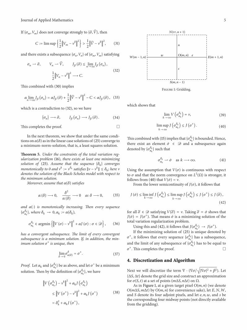
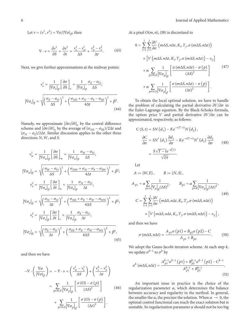
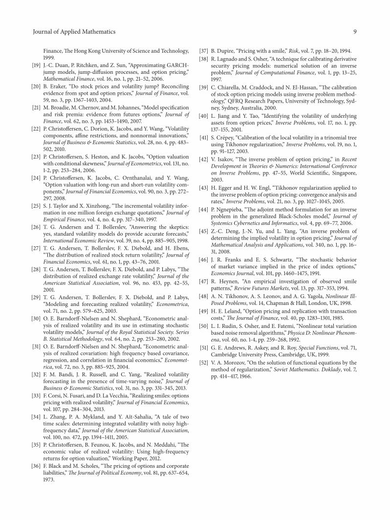