HAL Id: hal-02876965https://hal-normandie-univ.archives-ouvertes.fr/hal-02876965

Submitted on 10 Feb 2021

HAL is a multi-disciplinary open accessarchive for the deposit and dissemination of sci-entific research documents, whether they are pub-lished or not. The documents may come fromteaching and research institutions in France orabroad, or from public or private research centers.

L’archive ouverte pluridisciplinaire HAL, estdestinée au dépôt et à la diffusion de documentsscientifiques de niveau recherche, publiés ou non,émanant des établissements d’enseignement et derecherche français ou étrangers, des laboratoirespublics ou privés.

Reproductive health, fairness, and optimal policiesJohanna Etner, Natacha Raffin, Thomas Seegmuller

To cite this version:Johanna Etner, Natacha Raffin, Thomas Seegmuller. Reproductive health, fairness, and optimalpolicies. Journal of Public Economic Theory, Wiley, 2020, 22 (5), pp.1213-1244. �10.1111/jpet.12436�.�hal-02876965�

Reproductive health, fairness, and optimal policies

Johanna Etner1, Natacha Raffin1,2, Thomas Seegmuller3

1EconomiX, Université Paris Nanterre,CNRS, Nanterre, France2CREAM, Université Rouen Normandie,Rouen, France3CNRS, EHESS, Centrale Marseille, AMSE,Aix‐Marseille University, Marseille, France

CorrespondenceNatacha Raffin, CREAM, Université RouenNormandie, Rouen 76000, France.Email: natacha.raffin@univ-rouen.fr

Abstract

We consider an overlapping generations economy in which agents differ through their ability to procreate. Ex‐ante infertile households may incur health ex-penditure to increase their chances of parenthood. This health heterogeneity generates welfare inequal-ities that deserve to be ruled out. We explore three different criteria of social evaluation in the long‐run: the utilitarian approach, the ex‐ante egalitarian cri-terion and the ex‐post egalitarian one. We propose a set of economic instruments to decentralize each solution. To correct for the externalities and health inequalities, both a preventive (a taxation of capital) and a redistributive policy are required. We show that a more egalitarian allocation is associated with higher productive investment but reduced health expenditure and thus, lower population growth.

1 | INTRODUCTION

The state of human reproductive health has been one important debate in medical sciences inrecent years. The issue raised by a bench of papers concerns the natural ability for a couple tohave a child since it has been observed that infertility affects around 9% of procreating‐agedcouples worldwide (Inhorn & Patrizio, 2015).

Regarding this question, we draw the reader's attention that it differs from fertility issuesgenerally addressed in the economic literature. Indeed, following the Barro‐Becker analysis(1989), a huge literature has developed on the economic determinants of fertility, that is thenumber of children a household chooses to have. Some papers, among others, have focused onthe quality‐quantity trade‐off to justify the negative relationship between fertility and economicgrowth; others dealt with the development of a unified growth theory that allows to understand

1

the demographic transition (Galor & Weil, 2000); others are more interested in fertility dif-ferentials to better figure out economic inequalities (De la Croix & Doepke, 2003). In this paper,we study equity in a model with undesired infertility.

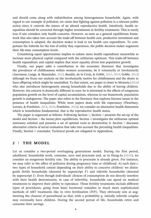
Our concern focuses on biological impairments that prevent couples to reproduce, based onrelevant measures of human fertility, independently from individual choices. The deteriorationof human reproductive health has been widely documented from a functional perspective in theepidemiological literature. Many studies point out the decline in men semen quality since thebeginning of the 20th century, the expanding Time To Pregnancy or the prevalence of newfemale complex reproductive disorders (like endometriosis, ovarian quality, etc.), independentof the age‐related natural decline in women fertility. For instance, following the seminal paperby Carlsen, Giwercman, Keiding, and Skakkebk (1992) that gave birth to the famous “fallingsperm counts” story, many studies have established a global declining quality of the sperma-togenis. Figure 1 illustrates some trends established in the literature, using one specific bio‐marker for male fertility. As for women reproductive health, there are ongoing research withrespect to the use of bio‐markers like antral follicular count and antimuëllerian hormone(Nelson, 2013). Meanwhile, a recent epidemiological literature has studied the prevalence ofendocrine disorders like polycystic ovarian symptoms (PCOs) or diagnosed endometriosiswhich are among the main causes of infertility. For instance, March et al. (2010) show thatPCOs are diagnosed for around 15% or more of reproductive‐aged women.

All these compelling evidence raise concerns that the reproductive health at a couple levelcould fall below some threshold levels that could impact fecundity, since those bio‐markers anddiseases are suitable indicators of chances to parenthood. In addition and crucial to our ana-lysis, these studies that point out a rapid change in human reproductive health cover periods offast economic development. Hence, we argue that postindustrial societies have created thepotential for increasing the exposure to specific lifestyle factors that might impair reproductivehealth. Among them, one can identify pollution or diet that might contribute to explainthe current worldwide infertility and came along with the development process. We may find inthe epidemiological literature many studies to support our view and that have long suggested

FIGURE 1 Evolution of sperm concentration. Data from Borges et al. (2015), Carlsen et al. (1992), Huanget al. (2017), Lackner et al. (2005), Levine et al. (2017), Rolland et al. (2013), Romero‐Otero et al. (2015)

2

adverse effects of exposure to environmental contaminants, such as persistent organic pollu-tants, on men and women reproductive health.1

Moreover, parenthood is a source of well‐being and we should be concerned that somecouples can not reproduce.2 To satisfy their desire of parenthood, some agents may becompelled to use costly medical services like Assisted Reproductive Technology (ART). Forinstance, since 2000, ART cycles annually grows by 5%–10% in developed countries (Kupkaet al., 2016). This reduced ability to conceive children may be also costly to overcome for thesociety. As shown by Chambers, Sullivan, Ishihara, Chapman, and Adamson (2009), the useof ARTs represents substantial out‐of‐pocket health expenses. The estimated cost of astandard in vitro fecundation (IVF) cycle ranges from 28% of Gross National Income (GNI)per capita in the United States to 10% of GNI per capita in Japan. Also before any publicpolicy, the gross cost of a standard IVF cycle ranges from 50% of an individual's annualdisposable income in the United States, approximately 20% in the UK, Scandinavian coun-tries and Australia, to 12% in Japan.

In our paper, we propose to explore the welfare inequalities induced by a health het-erogeneity since infertility entails a loss of utility. What matters to us is the unfair feature ofsuch a health heterogeneity because agents are not totally responsible for their reproductivehealth status. This is true if we think, for instance, to intra‐utero pollution exposure or livingconditions during childhood. We consider an overlapping generations model in which thedevelopment process generates an externality as a form of a health heterogeneity: two typesof households coexist within one generation, the fertile and infertile households. Moreover,ex‐ante infertile couples incur health treatments to increase their chances of parenthood.Hence, the laissez‐faire economy is characterized by several externalities: beyond theoligodendrocytes (OLG)‐induced inefficiency, the accumulation of capital slackenspopulation growth meanwhile health care spending create positive external effects on thedemographic dynamics.

We aim at discussing the efficient way to correct these externalities in the long term. At first,we consider the usual utilitarian social objective, but in contrast to Renström and Spataro(2019), we do not restrict our attention to a welfarist approach, even though they enrich it witha critical level of utility. Indeed, in the utilitarian case, health inequalities still prevail and wecan be concerned that the utility of the fertile is larger than the utility of the ex‐ante infertile.Because heterogeneity is not the result of any actions held by agents but rather due to cir-cumstances (let us refer for instance to pollution exposure), we also explore alternative criteriaof social evaluation according to Fleurbaey (2008), Ponthière (2016), or Fleurbaey, Leroux,Pestieau, Ponthière, and Zuber (2018). More precisely, we consider an inequality averse socialplanner who either maximizes the expected long‐run well‐being of the worst‐off (ex‐ante ega-litarian social criteria) or maximizes the long‐run realized well‐being of the worst‐off (ex‐postegalitarian social criteria).

Our results drive us to formulate some policy recommendations. To rule out inefficiencies,capital accumulation should be taxed. We argue that this preventive policy should be favored

1See for instance Mendola, Messer, and Rappazzo (2008), Recio‐Vega, Ocampo‐Gomez, Borja‐Aburto, Moran‐Martinez,and Cebrian‐Garcia (2008), Perry et al. (2011), Martenies and Perry (2013), Slama et al. (2013), Mehrpour, Karrari,Zamani, Tsatsakis, and Abdollahi (2014), Zhou et al. (2014), Chiu et al. (2015), Bolden, Rochester, Schultz, andKwiatkowski (2017), or Sifakis, Androutsopoulos, Tsatsakis, and Spandidos (2017).2The distress associated with subfertility or treatments of infertility causes induces substantial sociopsychological costs,like a severe degradation of self‐esteem, syndromes of depression, loss of gender identity, self‐assessed social pressurefrom families, friendships, and so forth (Greil, 1997; Moura‐Ramos, Gameiro, Canavarro, & Soares, 2012).

3

and should come along with redistribution among heterogeneous households. Again, withregard to our example of pollution, we claim that fighting against pollution is a relevant publicaction since it controls the source of an altered reproductive health. Intuitively, health in-equalities should be corrected through higher investments in fertility treatments. This is surelytrue if one considers only health concerns. However, as soon as a general equilibrium frame-work that also takes into account the trade‐off between health care, productive investment andconsumption is adopted, the decision maker is lead to tax health care expenditure. To com-pensate the Infertile for the loss of utility they experience, the public decision maker augmentstheir life‐time consumption levels.

Considering equal opportunities implies to reduce more health expenditure meanwhile toincrease more physical capital compared with the utilitarian optimum. This trade‐off betweenhealth expenditure and capital implies that more equality drives less population growth.

Finally, our paper adds a contribution to the economic literature that investigatesthe prevalence of childlessness within western economies, be it voluntarily or involuntarily(Aaronson, Lange, & Mazumder, 2014; Baudin, de la Croix, & Gobbi, 2015, 2019; Gobbi, 2013)although we focus our analysis on the involuntarily motive for childlessness and the desire tohave offspring which might be unsatisfied. To that extent, our paper is closer to Momota (2016)who also introduces heterogeneity among households due to the ability of having children.However, his concern is drastically different to ours: he is interested in the effects of exogenouspopulation growth on the level of capital accumulation, whereas in our framework, populationgrowth is endogenous. The paper also refers to the literature that explores fairness issues in thepresence of health inequalities. While most papers deals with life expectancy (Fleurbaey,Leroux, & Ponthière, 2014, 2016; Ponthière, 2016), we consider an alternative health dimensionwhich is nonetheless fundamental, that is the reproductive health status.

The paper is organized as follows: Following Section 1, Section 2 presents the set‐up of themodel and Section 3 the laissez‐faire equilibrium. Section 4 investigates the utilitarian optimalstationary solution and presents a set of optimal tools to decentralize it. Section 5 discussesalternative criteria of social evaluation that take into account the prevailing health inequalities.Finally, Section 6 concludes. Technical proofs are relegated to Appendices.

2 | THE MODEL

Let us consider a two‐period overlapping generations model. During the first period,adulthood, households work, consume, save and procreate and, as in Hung‐Ju (2018), weconsider an exogenous fertility rate. The ability to procreate is already given. For instance,we may refer to the effect of pollution during pregnancy time or childhood. At each date t ,two types of household coexist depending on their ability to conceive children: we distin-guish fertile households (denoted by superscript F) and infertile households (denotedby superscript I ). Even though individuals' choices of consumption do not directly interferewith their health determinants, in case of infertility, households can spend on medicaltreatments to improve their ability to reproduce. These fertility treatments include differenttypes of procedures, going from basic hormonal remedies to much more sophisticatedmethods of ART treatments like in vitro fertilization (IVF). They obviously aim at aug-menting the chances of parenthood so that, with a probability q, initially infertile couplesmay eventually have children. During the second period of life, households retire andconsume their savings.

4

2.1 | Demography

The proportion of fertile households within the population is denoted by πt (the proportion ofinfertile ones equals π(1 − )t ). This probability to be fertile is randomly distributed among thepopulation. The total number of children born at date t equals the number of children of fertilehouseholds (N nπt t) plus the number of children of successfully treated infertile households(N n π q(1 − )t t t), where n denotes the exogenous number of children each couple may have andNt is the size of the adult generation at date t . Hence, the adult population, that is, the laborforce evolves overtime according to

N N n π π q= × × [ + (1 − ) ].t t t t t+1(1)

2.2 | Households

During the first period of life, households i derive utility from current consumption (cti) as well

as parenthood (v) :U c v( , ˜)ti . When old, they derive utility from future consumption

d u d( ) : ( )ti

ti

+1 +1 . They do not choose the number of children they have, fertility is exogenous,although they might suffer from not being able to procreate. We consider a state‐dependentutility function since households face a health risk linked to their ability to conceive, v can taketwo values: v with probability qt and 0 with probability q1 − t. Their preferences are representedby an expected utility function:

( )( ) ( )

( ) ( ) ( )EU c d v

U c v δu d i F

q U c v q U c δu d i I, , =

, + , if = ,

, + (1 − ) , 0 + , if = .

iti

ti

tF

tF

t tI

t tI

tI

+1

+1

⎧⎨⎪⎩⎪

(2)

Following Aaronson et al. (2014), Baudin et al. (2015, 2019), we consider the followingspecifications. On the one hand, the utility function is given by U c v u c v( , ˜) = ( ) + ˜t t , withu z z( ) = lnt t.

3 On the other hand, the probability for a treatment to be successful writes:q x( ) =t

ax

x1 +t

t, with a 1⩽ and xt denotes the level of health care expenditure. The parameter a

merely accounts for the efficiency of the available medical technology or, equivalently, the levelof scientific medical knowledge.

Let us now present the budget constraints faced by households. For ease of presentation, weright now introduce a set of policy instruments that will be useful in the following. Duringadulthood, each household is endowed with one unit of labor inelastically offered to firms forwhich it receives the prevailing competitive wage, wt.

4 In addition, it might benefit from adifferentiated lump‐sum transfer, Tt

i. The net total income can be shared among current con-sumption, saving, st

i, and possibly for infertile households, health care. During retirement, eachcouple consumes the net income which equals the revenue from saving minus a transfer, θt+1.For both types of household, the first period budget constraint can be expressed as follows:

3We assume so far that parenthood does not impact the marginal utility of consumption. We discuss this assumption inSection 4.4Notice that here the health status does not affect productivity at work. Also, to keep the analysis as simple as possible,we do not introduce rearing cost of children. Since the number of offspring is assumed to be constant, enriching theanalysis with such a cost will not drastically alter our analysis.

5

c s w T+ = + ,tF

tF

t tF (3)

c s σ x w T+ + (1 − ) = + ,tI

tI

t t t tI (4)

where σt is the health policy instrument. The second period budget constraints write:

d R s θ i F I= − , for = , ,ti

t ti

t+1 +1 +1(5)

where we assume a complete depreciation of capital and we define R ρ r(1 − )t t t+1 +1 +1≡ , with ρta proportional tax on capital income.

2.3 | Government

At each date t , the government provides transfers to the young generation and can subsidyhealth expenditure thanks to a tax on capital and a lump‐sum tax on the old. The balancedbudget constraint of the government is given by:

( ) ( )N θ ρ r π s π s N π T π T N σ π x+ + (1 − ) = + (1 − ) + (1 − ) .t t t t t tF

t tI

t t tF

t tI

t t t t−1 −1 −1 −1 −1⎡⎣ ⎤⎦ (6)

2.4 | Firms

One good is produced using both physical capital, Kt, and labor, Lt. We can immediately defineper capita variables: y Y L= /t t t, k K L= /t t t. Again, to obtain tractable results, we assume a fairlystandard Cobb–Douglas production function:

y k=t tα (7)

with α0 < < 1/2. Being given the price of capital (rt) and the competitive wage (wt), theoptimization program of firms yields:

r αk= ,t tα−1 (8)

w α k= (1 − ) .t tα (9)

2.5 | Reproductive health

As documented in Section 1, the development process generates a harmful externality thatnegatively affects the probability of being fertile. Since GDP per capita is a well‐establishedmeasure of development and it increases with capital per capita, we state that π π k= ( )t t andπ k′( ) 0⩽ so that, as one economy develops, the natural reproductive health declines. Weexplicit in further details our hypothesis about this endogenous probability of being fertile inAssumption 1:

Assumption 1. We assume that π is sufficiently close to 1 and ϵππ k k

π k

′( )

( )≡ is close to 0

with π k π k π π π′( ) 0 ″( ), (0) = > (+ ) > 00⩽ ⩽ ∞ .

6

This assumption means that the chances of parenthood are weakly decreasing with thestock of capital and sufficiently close to 1. If we interpret the relationship between π and k asthe effect of pollution on couples reproductive health, Assumption 1 seems in accordance withthe empirical literature.

Within this framework, we can now analyze the static choices made by households and theninvestigate the long‐run behavior of this economy.

3 | THE LAISSEZ ‐FAIRE ECONOMY

This section defines the inter‐temporal equilibrium in the laissez‐faire economy, the levels ofpolicy instruments, T σ θ, ,t

it t+1, and ρt+1, being set to zero. The equilibrium, given the variables

from the previous period, can be defined by a wage rate wt and a gross rate of return Rt,aggregate variables K L,t t, and Yt and individuals variables, c s c s, , ,t

FtF

tI

tI , and xt.

3.1 | Households' choices

Households maximize their expected utility (2) under the budget constraints (3)–(5) and a positivityconstraint, x 0t ⩾ . We derive from the first‐order conditions, the trade‐off between young and oldconsumptions and the trade‐off between health and consumption for the Infertile:

c

δR

di F I

1= , for = , ,

ti

t

ti

+1

+1

(10)

c

av

xx

1

(1 + ), with an equality if > 0.

tI

tt2

⩾ (11)

Fertile households do not spend on health care and we can easily deduce their optimal levelof saving, which is increasing with labor income:

sδ

δw s k=

1 +( ),t

Ft

Ft≡ (12)

with s k( ) > 0Ft

′ . As for the Infertile, let us note that if x = 0t , then

sδ

av.t

F ⩽ (13)

This inequality implies that the loss of utility from a low level of consumption dominates thepotential welfare gain associated with an improved reproductive health. Hence, since the utilityfunction defined over consumption is concave, this inequality is verified all the more thatconsumption levels are initially low. We can state that for low incomes, it is more likely thathouseholds do not invest in fertility treatments. In that configuration, s s=t

ItF . On the contrary,

if Equation (13) is not satisfied, x > 0t and, using Equation (12), we get the optimal saving andhealth expenditure for infertile households:

7

s s kδ

δx= ( ) −

1 +,t

I Ft t

(14)

xav

δs(1 + ) = .t tI2 (15)

Solving the system (14)–(15), we deduce the expression of xt and stI as functions of kt:

x x kav α

δk A A A

av

δ( ) =

(1 − )

1 +− 1 + − , with 1 +

2(1 + ),t t t

α 2≡ ≡ (16)

and

s s kδ x k

av( ) =

(1 + ( )),t

I It

t2

≡ (17)

where x k′( ) > 0t and s k( ) > 0It

′ .

3.2 | Labor market

On the labor market at date t , the supply of labor Nt being inelastic and the demand Lt being thesolution to Equation (9), we get that:

L N N n π k π k q x k= = × × [ ( ) + (1 − ( )) ( ( ))].t t t t t t−1 −1 −1 −1(18)

3.3 | Capital market

The clearing condition on the capital market entails that the supply of saving by the youngequals the capital used by firms:

K N π k s k π k s k= [ ( ) ( ) + (1 − ( )) ( )].t t tF

t tI

t+1(19)

Using Equation (18), we derive the dynamics of capital–labor ratio:

kπ k s k π k s k

n x k k=

( ) ( ) + (1 − ( )) ( )

Γ( ( ), ),t

tF

t tI

t

t t+1

(20)

where x k k π k π k q x kΓ( ( ), ) = [ ( ) + (1 − ( )) ( ( ))]t t t t t and n x k kΓ( ( ), )t t is the endogenous growthfactor of the population size of generations. The accumulation of physical capital induces twoopposite effects on population growth: a negative direct effect through the increase in thenumber of infertile households and a positive indirect effect through health expenditure. Whenthe negative effect dominates, physical capital accumulation entails a negative dilution effect5,otherwise a positive one. In addition, physical capital accumulation impacts global saving,through three channels: (a) it affects the distribution of infertile and fertile households withinthe population; (b) it increases savings for each type of household; (c) it triggers more health

5Recall that the dilution effect corresponds to a decrease of per capita variables following an increase in the labor forceor, equivalently, in the population growth.

8

expenditure and thus involves an eviction effect on the Infertile's saving. The global dynamics ofthe economy depends on the magnitude of each mechanism.

Given k K L= / 00 0 0 ⩾ , the inter‐temporal equilibrium is a sequence k{ }t that satisfies con-dition (20) for all t 0⩾ . A steady state with x > 0, if it exists, is a solution k that solves the abovedynamic Equation (20) evaluated at the steady state, so that k k k= =t t+1 . The existence anduniqueness of such a steady state is characterized in the following proposition.

Proposition 1. Under Assumption 1 and if v sufficiently large, so that

v vδ

a α

α δ

δ nπ> ˜

1 +

(1 − )×

(1 − )

(1 + ) (0),

αα

−1−⎡

⎣⎢⎤⎦⎥

⎡⎣⎢

⎤⎦⎥≡

there exists a unique steady state, k, such that health expenditure is strictly positive (x > 0).

Proof. See Appendix A. □

We show that, in the long term, the economy reaches a stationary state in which infertilehouseholds do spend on fertility treatments if the benefit of parenthood is large enough. Indeed,investing in ARTs to augment the chances of parenthood is costly and induces an eviction effecton saving. Nevertheless, by increasing the share of procreating households, the demographicgrowth is boosted.

4 | THE CLASSICAL UTILITARIAN WELFARE ANALYSIS

Our model is characterized by several inefficiencies that we identify now. First, accumulatingphysical capital induces a negative externality as it increases the probability to be infertile anddecreases the one to be fertile. This implies a lower utility for each generation. But beyond this,physical capital creates an additional externality because more physical capital means less populationgrowth. Simultaneously, since households may spend on health care, there exists a third externality,because health expenditure also influence the population growth factor. Finally, because of theoverlapping generations, the intergenerational allocation at the equilibrium can be suboptimal. Ofcourse, all these externalities are relevant at an inter‐temporal equilibrium as well as at a steady state.In this set‐up, we aim at exploring what would be a first‐best optimal allocation. To that end, wepropose a welfare analysis using a classical utilitarian criterion of social evaluation and we char-acterize the optimal solution. Then, we provide some policy recommendations to correct the in-efficiencies and discuss the nature of the economic policy.

4.1 | The utilitarian social optimum

The utilitarian social planner maximizes a Millian social welfare objective that takes into account theaverage expected utility,6 SWU . In this context of endogenous population, we assume that she doesnot grant any particular weight to the overall size of the population but rather the average level of

6See Blackorby, Bossert, and Donaldson (2005) for a discussion of the social welfare criteria when the population isendogenous.

9

utility is maximized. To derive clear cut results and compare them with the laissez‐faire economy, wefocus our analysis on the stationary solution. To comply with her goal, the social planner chooses theoptimal levels of consumption c c d d( , , , )F I F I , health expenditures x( ), and physical capital k( ),under the two constraints of resources and positivity for health care expenditure. The program of theutilitarian central planner can thus be written as follows:

SW π k c δ d v

π k c δ dax

xv

s t k π k c π k c x

π k d π k d

n x knk x k

x

max ( )[ln + ln + ]

+ (1 − ( )) ln + ln +1 +

,

. . ( ) + (1 − ( ))( + )

+( ) + (1 − ( ))

Γ( , )+ Γ( , )

0.

c c d d x k

U F F

I I

α F I

F I

, , , , , ,F I F I

⎧

⎨

⎪⎪⎪⎪

⎩

⎪⎪⎪⎪

⎡⎣⎢

⎤⎦⎥

≡

⩾

⩾

First of all, at the optimum, expected marginal utilities of consumption are equalized and thusconsumption levels should be equalized among heterogeneous agents, c c c d d d= = , = =* *F I F I .7

Then we already depart from the laissez‐faire choices of consumption and we confirm that a policyshould be implemented to reach the optimal utilitarian solution. Second, we derive the optimaltrade‐off between young and old consumption over the life‐cycle:

δcd

n x k=

Γ( , ).*

*

* *(21)

The marginal rate of substitution between young and old consumption is equal to theoptimal population growth factor, n x kΓ( , )* * .8 Third, we consider the trade‐off between con-sumption and health:

av

x

δa

x x k c

nk a

c x

μ

π k(1 + )+

(1 + ) Γ( , )=

1+

(1 + )−

1 − ( ),

* * * * *

*

* *

*

*2 2 2(22)

where μ is the Lagrange multiplier associated to the positivity constraint on x . There exists aninterior optimal solution for health expenditure when the marginal social welfare gain from in-vesting in health equals the marginal social welfare loss. On the one hand, the marginal socialwelfare gain consists in a pure utility gain from parenthood plus a reallocation of resources withingenerations, through the reduced weight granted to old households' consumption. On the otherhand, the marginal social welfare loss is the foregone consumption added to the required increase inthe productive investment. Finally, we deduce the trade‐off between generations, which is given by

α k n x k π k x

c π kax

x

nk

c

δ

x kv

( ) = Γ( , ) − ′( )

+ ′( ) 1 −1 +

−Γ( , )

− .

* * * * *

* **

*

*

* * *

α−1

⎜ ⎟⎡⎣⎢

⎛⎝

⎞⎠

⎛⎝⎜

⎞⎠⎟

⎤⎦⎥

(23)

7Superscripts * indicate the utilitarian optimal solution. See Appendix B for more details.8Notice that our results are robust to alternative specification of separable utility functions, like CES between young and

old consumption: U c d v v δ( , , ) = + + .t tc

ϵ

d

ϵ

( )

1−

( )

1−t

ϵt

ϵ1−+1

1−

10

This condition is in fact a modified golden rule. If the probability to be fertile were constant,then we would have obtained a standard golden rule, except for the presence of the growthfactor. As soon as the capital externality occurs, additional and potentially opposite effects arise.Keeping in mind that investment and production are related, more capital means less popu-lation, lowering the cost of productive investment. Nevertheless, more capital induces moreinfertile households and thus lowers the social welfare. This last negative effect mitigates theformer incentives to accumulate physical capital.

Using these arbitrages, we can also study the existence and the properties of the utilitarianoptimal allocation. In particular, although we do not know whether the optimal level of healthexpenditure is higher than the laissez‐faire one, we can show that it should be strictly positive.This is stated in Proposition 2 below:

Proposition 2. Under Assumption 1 and v sufficiently large, there exists a uniqueoptimal allocation x k( , )* * with x > 0* .

Proof. See Appendix C. □

As discussed previously, we could consider the case where parenthood affects the marginalutility of consumption. Let us now consider the utility function for a fertile and infertile agentrespectively, as follows:

( )( ) ( )

( ) ( ) ( )EU c d v

U c v δu d i F

q U c v q U c δu d i I, , =

, + , if = ,

, + (1 − ) , 0 + , if = ,

iti

ti

tF

tF

t tI

t tI

tI

+1

+1

⎧⎨⎪⎩⎪

(24)

where U c v U c v( , ) > 0, ( , ) 0ti

ti

1 11 ⩽ and u d( )ti is increasing and concave in dt . We deduce from

Appendix D that, at the optimum, d d d= =* * *I F . We also show that

q x U c v q x U c U c v( ) ( , ) + (1 − ( )) ( , 0) = ( , )I I F1 1 1

(25)

Consequently, we have

U c v U c v U c U c v( , ) − ( , ) 0 ( , 0) − ( , ) 0F I I I1 1 1 1⪌ ⇔ ⪌ (26)

Or,

c c U 0F I12⪌ ⇔ ⪌

In the case of a state‐dependent utility, the role played by correlation aversion/loving (firstintroduced by Richard, 1975; see also Eeckhoudt, Rey, & Schlesinger, 2007, for multivariate riskpreferences) is crucial. Correlation loving corresponds, in health economics, to the com-plementarity between wealth and health while correlation aversion refers to a subsitutabilitybetween the two.9 In our set‐up, ifU < 012 , the marginal utility of consumption is higher in the

9Correlation aversion implies that an individual prefers to disaggregate fixed reductions in health and consumption.Notice that correlation aversion—that is an individual prefers to disaggregate harms—in the case of one attribute meansthat she is risk averse.

11

case of no parenthood: individuals are correlation averse. In that case, the central planner givesmore to the Infertile to obtain a higher level of welfare. If U > 012 , the marginal utility ofconsumption is higher in the case of parenthood: individuals are correlation prone. To increasewelfare, the central planner gives more to the Fertile. Of course, if U = 012 , levels of con-sumption are identical for both types of household. To our knowledge, there is no empiricalsupport and/or theoretical justification for one particular assumption. Nevertheless, Attema,L'haridon, and van de Kuilen (2019) recently find empirical evidence of correlation aversion forgains in health and wealth. Following their work, our results would not change significantly.

Once we have described the optimal utilitarian solution, we naturally wonder how to reachit in the market economy. To do so, we derive again the decentralized optimal choices for bothtypes of household once policy instruments are enforced and we compare them with theutilitarian optimal solution. We can then discuss the optimal design of the public policy to beimplemented, according to the preferences of the social planner.

4.2 | The utilitarian optimal policy

In an OLG framework, we need first to correct the inefficient level of capital. To reach thegolden rule, a proportional tax on capital, ρ, is implemented. Moreover, to ensure the budget isbalanced at each period, lump‐sum transfers to the old, θ, are enforced. Second, considering areproductive health issue introduces heterogeneity among households and displays an externaleffect on population growth. Therefore, two adding instruments are required to restore op-timality: a distortionary subsidy on health expenditure (σ) and a lump‐sum transfer toward theyoung (Ti). Notice that the capital externality that shapes the distribution of the Fertile and theInfertile within the population is corrected through the appropriate distortionary tax on capital.The following proposition summarizes our results.

Proposition 3. Consider that Assumption 1 holds, δ small and v sufficiently large, theutilitarian social optimum can be decentralized by means of the following instruments:

(i) A tax on capital income, ρ = 1 − (0, 1)*n

α k

Γ

( )

*

* α−1 ∈ ;(ii) A tax on health expenditure, σ < 0* , such that ( )= − < 0

σ

σ v

δ nk

c1 −

1

Γ

*

* *

*

*;

(iii) Differentiated lump‐sum transfers between the Fertile and the Infertile, T *F and T *I ,satisfying T = 0*F and T σ x= (1 − ) > 0* * *I ;

(iv) A positive lump‐sum tax on the old, θ > 0* , to balance the government's budget.

Proof. See Appendix E. □

The positiveness of θ* involves a taxation of old households' consumption. This generatesfiscal resources meanwhile it incites young households to save more. This capital accumulationis the source of the externality that should be corrected. Hence, the government implements aproportional tax on capital income to ensure the achievement of the “adjusted” golden rule (seeEquation (23)). In addition, this capital accumulation generates more consumption and allowsinfertile households to afford for more and more fertility treatments. It reinforces the hetero-geneity between the two groups. To enforce the optimal level of health expenditure, we showthat a tax on health care is required. Nevertheless, to guarantee that consumption are identicalamong the two types of households, positive transfers toward the young should be

12

differentiated. This result might be at first sight surprising and counter‐intuitive; However, letus re‐examine the infertile households' budget constraint: c σ T x x s w+ (1 − − ) + =I I I∕ .Taking into account the redistribution effect through TI , the health policy design can besummarized by a unique variable t x σ T x( ) + /I≡ . At the utilitarian optimum, we easily seethat t x( ) > 0.10 Overall, infertile couples are well subsidized by the government.

To sum‐up, the optimal public policy design includes redistribution and a tax on physicalcapital that should be interpreted as a preventive policy tool. But a public health policy thatreduces the cost of ARTs is not relevant to reach the optimum. For instance, if we follow‐upwith our example of pollution, the authorities should favor the reduction of polluting emissionsthat alter couples reproductive health and ensure that infertile households can derive suffi-ciently high expected utility all over their life‐cycle, through both consumption and parenthood.

4.3 | Discussion

Using a classical utilitarian criterion, the instruments to decentralize the social optimum allow toreduce inequalities among the two social groups—the Fertile and the Infertile—through theequalization of consumptions and the reduction of the capital externality. Nonetheless, the optimalpolicy does not eradicate the source of health inequality but may compensate for it by subsidizingthe Infertile and enforcing an identical level of consumption. We can still be concerned with suchan approach since the utility of the Fertile is larger than the expected utility of the Infertile. Inaddition, if we consider that the risk of fertility agents are exposed to is not the consequence of anyaction, but rather due to circumstances, then this health heterogeneity appears to be unfair. It istypically the case of pollution exposure for which agents can not be blamed a priori. In thefollowing sections, we explore alternative criteria of social evaluation for which the social plannerexhibits inequality aversion. We then assess the optimal design of the public policy that should beimplemented, in comparison with the utilitarian solution.

5 | INEQUALITY AVERSION CRITERIA

The capital externality generates a distribution on the two types of households and this createsdifferent outcome prospects. Even if, for the social observer, the ability to reproduce is viewed asrandom, the fact that it is antecedent to the decision process suggests that it should be consideredas circumstances. According to the “compensation principle” (see Fleurbaey, 2008; Pon-thière, 2016), such type of inequalities, due to circumstances, should be eliminated as much aspossible. In addition, in our set‐up, the random consequence of fertility treatments generates another type of heterogeneity among the Infertile. Then, we distinguish two sources of healthinequalities that deserve to be handled. To do so, we rely on two approaches developed in theeconomic literature: the ex‐ante inequality aversion and the ex‐post inequality aversion. In the firstcase, the social planner focuses on the differences between social groups defined by the same set ofcircumstances (here, the Fertile and the Infertile) while, in the second case, she considers theunequal outcome among individuals who exert the same effort (here the Infertile). These twoapproaches seem to be relevant in the case of this twofold dimension of health inequality.

10Since σ < 0 and T t x> 0, ( )I is strictly decreasing and there exists x T σ= − / > 0I such that t x( ) > 0 for x x< andt x( ) < 0 for x x> .

13

5.1 | Ex‐ante egalitarian criterion

Let us first consider a social planner who adopts an ex‐ante egalitarian criterion of the socialwelfare evaluation. This social objective implies to select the allocation that maximizes theexpected lifetime well‐being of the worst‐off social group, the ex‐ante infertile households. Thesocial welfare function is:

SW EU c d v EU c d vmin{ ( , , ), ( , , )},E F F F I I I≡

where EU c d v c δ d v( , , ) = ln + ln +F F F F F and EU c d v c δ d v( , , ) = ln + ln +I I I I I ax

x1 +.

It is possible to rewrite this problem as the maximization of the expected utility of the ex‐ante Infertile, conditionally on the resource constraint of the economy, the positivity constrainton x and, conditionally on the egalitarian constraint so that ex‐ante infertile households are notworse‐off than fertile households.

c δ dax

xv

s t k π k c π k c x

π k d π k d

n x knk x k

x

c δ d v c δ dax

xv

max ln + ln +1 +

,

. . ( ) + (1 − ( ))( + )

+( ) + (1 − ( ))

Γ( , )+ Γ( , )

0,

ln + ln + = ln + ln +1 +

.

c c d d x k

I I

α F I

F I

F F I I

, , , , ,F I F I

⎧

⎨

⎪⎪⎪⎪

⎩

⎪⎪⎪⎪

⩾

⩾

As usual, at the optimum,11 we can write the trade‐off between young and old consumptionover the life‐cycle:

δcd

n x ki F I=

Γ( , )for = , .iE

iE

E E(27)

Like in the utilitarian solution, the marginal rate of substitution between life‐time con-sumptions is equal to the optimal population growth factor, n x kΓ( , )E E . Nevertheless, contraryto the utilitarian optimal solution, consumption levels are not equalized among heterogeneoushouseholds. Indeed, we can show that:

cξ

ξ

π k

π kc d

ξ

ξ

π k

π kd=

1 −

1 − ( )

( )and =

1 −

1 − ( )

( ),FE

E

E

E

EIE FE

E

E

E

EIE (28)

with ξ E the Lagrange multiplier associated to the egalitarian constraint and ξ π k< ( )E E .Consequently, we deduce that c c<FE IE and d d<FE IE and thus the situation is indeed reversedcompared to the laissez‐faire economy.

Second, we obtain a similar trade‐off between consumption and health compared with theutilitarian one:

av

x

δa

x x k

π k

ξ c

nk a

c x

μ

ξ(1 + )+

(1 + ) Γ( , )

1 − ( )

1 −=

1+

(1 + )−

1 −,

E E E E

E

E IE

E

IE E

E

E2 2 2(29)

11Superscripts E indicate the ex‐ante egalitarian solution. See Appendix F for more details.

14

with μE the Lagrange multiplier associated to the positivity constraint on x . Finally, the trade‐off between generations yields an alternative modified golden rule

α k n x k π k x

c π kax

x

nk

c

δ

x k

π k

ξ

c π k δξ

ξ

π k

π k

( ) = Γ( , ) − ′( )

+ ′( ) 1 −1 +

−Γ( , )

1 − ( )

1 −

+ ′( )(1 + )1 −

1 − ( )

( )− 1 .

E α E E E E

IE EE

E

E

IE E E

E

E

IE EE

E

E

E

−1

⎛⎝⎜

⎞⎠⎟

⎡⎣⎢

⎛⎝⎜

⎞⎠⎟

⎤⎦⎥

⎛⎝⎜

⎞⎠⎟

(30)

Under this criterion, the weight granted to the Fertile (ξ E) is lower compared to the utili-tarian case (π k( )E ). By adapting the proof of Proposition 2, we can easily show that μ = 0E andthus an interior solution exists, x > 0E . Therefore, like in the utilitarian case, there is a uniquepair x k( , )E E that characterizes the ex‐ante egalitarian equilibrium. The consequences on theoptimal level of health expenditure and physical capital are given in the following proposition.

Proposition 4. Consider that Assumption 1 holds and v sufficiently large. Under theex‐ante egalitarian social criterion, the optimal level of health expenditure satisfies

x x0 < < *E and the optimal stock of capital k k> *E .

Proof. See Appendix F. □

A risk of fertility treatment still prevails because q x( ) is strictly lower than one. Thus, theexpected utility of parenthood is always smaller for infertile couples, q x v v( ) < . Therefore, toensure the equality of welfare for all households, the social planner allocates more life‐cycleconsumption to the Infertile and less to the Fertile. If ξ E were equal to π k( )E , consumptionlevels would be identical. Since ξ π k< ( )E E , it comes that the solutions differ so that c c> *IE

and d d> *IE . Moreover, since the weight granted to the Infertile is larger, it comes that theaggregate consumption is larger compared to the utilitarian case. To finance this augmentedaggregate consumption, the social planner invests more in productive capital, detrimental tohealth expenditure.

We can now discuss the design of the public policy required to decentralize the ex‐anteegalitarian social optimum.12 The expression of the proportional tax on capital is similar to theutilitarian one and one can also implement a positive lump‐sum transfer to the infertile youngonly, T = 0FE and T > 0IE . From the previous analysis, we can directly deduce that the tax onhealth expenditures is larger: σ x k σ x k− ( , ) < − ( , )* * E E . Since fertility treatments are not en-tirely efficient, the most relevant public action consists in a more generous redistributive policy,besides the taxation of the capital, that is the source of infertility.

5.2 | Ex‐post egalitarian criterion

Let us now consider an ex‐post egalitarian social planner who allocates the resources according tothe level of the realized well‐being of the worst‐off. Recall that in our framework, having children

12See Appendix G.

15

does not entail any cost since we focus on the loss of utility induced by infertility and fertility isexogenous. We assume that v is sufficiently large to ensure that the worst‐off group is composed ofagents who have invested in fertility treatment but for whom it was unsuccessful. Say differently, thecost of child bearing is relatively not significant compared with the benefit of having children(Moura‐Ramos et al., 2012). Ex‐ante Infertile households are identical before the success of fertilitytreatments is revealed and make similar decisions (c s x, ,I I ). Once the treatment is realized, there aretwo types of infertile households because some of them succeed (i IF= ) while some others do not(i II= ). The social planner corrects the treatment‐induced inequality between the two types ofinfertile households in terms of well‐being, focusing on the second period consumption (dIF and dII).Ex‐post, there are a priori three types of household in the economy. The realized utility of fertilehouseholds writes:U c d v c δ d v( , , ) = ln + ln +F F F F F ; the one of lucky InfertileU c d v( , , ) =IF I IF

c δ d vln + ln +I IF ; and, the one of unlucky InfertileU c d c δ d( , ) = ln + lnII I II I II .Taking into account the realized utilities of the three types of household, the social welfare

function writes:

SW U c d v U c d v U c d vmin{ ( , , ), ( , , ), ( , , )}.P F F F IF I IF II I II≡

Following the ex‐post egalitarian criterion, the objective of the social planner is to maximize theutility of ex‐post infertile households who have invested in health but for whom the treatment wasunsuccessful. We can write the optimization program conditionally on the resource constraint ofthe economy, the positivity constraint on x and the egalitarian constraints such that unluckyinfertile households are not worse‐off than lucky infertile and fertile households:

c δ d

s t k π k c π k c x

π k d π k q x d q x d

n x knk x k

x

c δ d v c δ d

c δ d v c δ d

max ln + ln ,

. . ( ) + (1 − ( ))[ + ]

+( ) + (1 − ( ))[ ( ) + (1 − ( )) ]

Γ( , )+ Γ( , )

0,

ln + ln + = ln + ln ,

ln + ln + = ln + ln ,

c c d d d x k

I II

α F I

F IF II

F F I II

I IF I II

, , , , , ,F I F IF II

⎧

⎨

⎪⎪⎪⎪

⎩

⎪⎪⎪⎪

⩾

⩾

As usual, at the ex‐post egalitarian optimum, we obtain the trade‐off between consumptionsover the life‐cycle:13

δcd

n x k=

Γ( , ),FP

FP

P P(31)

δcq x d q x d

n x k=

( ) + (1 − ( ))

Γ( , ).IP

P IFP P IIP

P P(32)

In addition, when the social planner is averse to ex‐post inequalities, we can establish thatconsumption levels for old unlucky infertile households are larger than the ones of fertile andfurther on old lucky infertile couples: d d d> >IIP FP IFP. We also find that c c>IP FP.

13Superscripts P indicate the ex‐post egalitarian solution. See Appendix H for more details.

16

Second, we derive the trade‐off between consumption and health expenditure

λ a π k

x

d

n x k

d

n x kδ

a π k

x x k

nk λ a π k

xλ π k μ

(1 − ( ))

(1 + ) Γ( , )−

Γ( , )+

(1 − ( ))

(1 + ) Γ( , )

=(1 − ( ))

(1 + )+ (1 − ( )) − .

P P

P

IIP

P P

IFP

P P

P

P P P

P P P

PP P P

2 2

2

⎛⎝⎜

⎞⎠⎟ (33)

where λP and μP are the Lagrange multipliers associated to the resources and positivity constraints.Finally, we obtain the trade‐off between generations

α k n x k π k c c x nk π kax

x

π k c π k c π kax

x

δ

x k

δ c c π kax

x

( ) = Γ( , ) + ′( )[ − − ] + ′( ) 1 −1 +

− ( ( ) + (1 − ( )) ) ′( ) 1 −1 + Γ( , )

− ( − ) ′( ) 1 −1 +

.

P α P P P FP IP P P PP

P

P FP P IP PP

P P P

IP FP PP

P

−1⎛⎝⎜

⎞⎠⎟

⎛⎝⎜

⎞⎠⎟

⎛⎝⎜

⎞⎠⎟

(34)

Proposition 5. Consider that Assumption 1 holds, v sufficiently large and δ sufficientlysmall. Under the ex‐post egalitarian social criterion, the optimal level of health expendituresatisfies x x x= 0 < < *P E and the optimal stock of capital k k k> > *P E .

Proof. See Appendix H. □

This criterion involves that the social planner rules out ex‐post inequalities among infertilehouseholds. Because the treatment is not perfectly efficient, the social planner chooses no treatmentin fertility (x = 0P ). Hence, ex‐post, there is only one type of infertile households, i II= . There isno longer households of type i IF= because q (0) = 0. In addition, to reduce inequalities betweenfertile and infertile households, the social planner distributes resources toward the Infertile'sconsumption all over the life‐cycle. To finance this increased consumption, she needs to investmore in physical capital. Since there is no health expenditure, she invests more in productivecapital compared to the previous criteria. Notice that if the worst‐off group would be the luckyInfertile (for instance due to costs of child bearing), it does not drastically modify our analysis, sincethe utility of the three types of household is equalized at the ex‐post egalitarian optimum.

Let us turn now to the design of the public policy to decentralize the ex‐post egalitarian socialoptimum.14 We can state that the tax on fertility treatment is sufficiently large to incite householdsnot to spend on health care. The expression of the other instruments are similar to the previous cases.

5.3 | Discussion

At the laissez‐faire, households do not enjoy the same level of utility. This social situation can beviewed as unfair. As seen in the previous section, at the utilitarian optimum, these inequalitiesare not considered, even if consumptions are equalized among households.

14See Appendix I.

17

As far as the social planner is concerned with the reduction of inequalities, we adoptwelfare criteria that aim to reduce these utility differentials. In the ex‐ante approach, the twosocial groups—the Fertile and the ex‐ante Infertile—have the same expected utility beforeone knows whether the treatment is successful. After the realization of the risk, three typesof households with three different realized levels of utility prevail. In the ex‐post approach,we take into account the realization of the utilities of the three types of household. Only twosocial groups—the Fertile and the ex‐post Infertile—persist in the second period, but theyhave the same realized utility. Even though we do not discuss the choice of the egalitariancriteria to be adopted, one can be interested in considering equal opportunities and comparethem with the utilitarian optimum. We have established that whatever the egalitarian cri-terion we use, health expenditure are reduced and investment in physical capital is increasedcompared with the utilitarian optimum. This also means that more equality implies lesspopulation growth and that there exists a trade‐off between egalitarism among individualsand population growth.

Intuitively, health inequalities should be corrected through higher investments in fertilitytreatments. This could be true if one considers only health concerns. We show that this is nomore true as soon as general equilibrium framework that also takes into account the trade‐offbetween health expenditure, productive investment, and consumption is adopted.

6 | CONCLUDING REMARKS

Based on epidemiological evidence, we assume that the development process impacts ne-gatively fertility. We analyze the implications of such a feature considering an OLG economywhere ex‐ante infertile households may incur health expenditure to increase their chances ofparenthood. We compare three long‐run optimal allocations, depending on the criteria ofsocial evaluation adopted by the planner. We claim that when the social planner does notexhibit any aversion to inequality, the optimal level of health expenditure is the highest one.When she displays inequality aversion, optimal health expenditure diminishes and is equalto zero when she focuses on the realized well‐being of the worst‐off social group. On thecontrary, the utilitarian optimal level of capital is the lowest one and the ex‐post egalitarianone is the largest. Then, we determine the optimal policy to decentralize each allocation. Weunderscore that to correct for the prevailing externality and the health inequality it induces,it is necessary to implement both preventive and redistributive policies, to globally subsidymostly harmed agents within the economy. More precisely, the tax on health expenditure is acrucial tool to reduce the heterogeneity and to rule out inequalities. Opposite to publicpolicies implemented in many countries which consist in subsidizing ARTs, we argue that toreduce inequalities, it is more appropriate to enforce redistribution and prevention. Forinstance, if infertility comes from pollution exposure, a fair health policy could be a taxationof polluting emissions. Our strong conclusions could be mitigated if we consider incomeheterogeneity besides health heterogeneity. In this case, we may justify a positive subsidizeto health expenditure that comes along with a preventive and redistributive policy. Thispaves the way to future research.

ACKNOWLEDGMENTSWe would like to thank participants to the Conferences Dyniper 2016, SURED 2016, PET 2018,and EAERE 2018 and ASSET 2018 for their helpful comments. This paper benefits from the

18

financial support of the French National Research Agency ANR‐17‐EURE‐0020, ANR‐15‐CE33‐0001‐01, and ANR‐16‐CE03‐0005. J. Etner thanks support from the Labex MME‐DII program.

ORCIDNatacha Raffin http://orcid.org/0000-0001-7279-4119

REFERENCESAaronson, D., Lange, F., & Mazumder, B. (2014). Fertility transition along the extensive and the intensive

margins? American Economic Review, 104, 1–25.Attema, A., L'haridon, O., & van de Kuilen, G. (2019). Measuring multivariate risk preferences in the health

domain. Journal of Health Economics, 64, 15–24.Barro, R., & Becker, G. (1989). Fertility choice in a model of economic growth. Econometrica, 57, 481–501.Baudin, T., de la Croix, D., & Gobbi, P. E. (2015). Fertility and childlessness in the United States. American

Economic Review, 105, 1852–1882.Baudin, T., de la Croix, D., & Gobbi, P. (2019). Endogenous childlessness and stages of development. Journal of

the European Economic Association, 18, 83–133.Blackorby, C., Bossert, W., & Donaldson, D. (2005). Population issues in social choice theory, welfare economics,

and ethics. Cambridge: Cambridge University Press.Bolden, A. L., Rochester, J. R., Schultz, K., & Kwiatkowski, C. F. (2017). Polycyclic aromatic hydrocarbons and

female reproductive health: A scoping review. Reproductive Toxicology, 73, 61–74.Borges, E., SouzaSetti, A., Paes de Almeida Ferreira Braga, D., de Cassia Savio Figueira, R., & Laconelli, A.

(2015). Decline in semen quality among infertile men in Brazil during the past 10 years. InternationalBrazilian Journal of Urology, 41, 757–763.

Carlsen, E., Giwercman, A., Keiding, N., & Skakkebk, N. (1992). Evidence for decreasing quality of semen qualityduring past 50 years. British Medical Journal, 305, 609–613.

Chambers, G. M., Sullivan, E. A., Ishihara, O., Chapman, M. G., & Adamson, G. D. (2009). The economic impact ofassisted reproductive technology: A review of selected developed countries. Fertility and Sterility, 91, 2281–2294.

Chiu, Y. H., Afeiche, M. C., Gaskins, A. J., Williams, P. L., Tanrikut, C., Hauser, R., & Chavarro, J. E. (2015).Fruit and vegetable intake and their pesticide residues in relation to semen quality among men from afertility clinic. Human Reproduction, 30, 1352–1341.

De la Croix, D., & Doepke, M. (2003). Inequality and growth: Why differential fertility matters. AmericanEconomic Review, 93, 1091–1113.

Eeckhoudt, L., Rey, B., & Schlesinger, H. (2007). A good sign for multivariate risk taking. Management Science,53, 117–124.

Fleurbaey, M. (2008). Fairness, responsibility and welfare. New York, NY: Oxford University Press.Fleurbaey, M., Leroux, M. L., & Ponthière, G. (2014). Compensating the dead. Journal of Mathematical

Economics, 51, 28–41.Fleurbaey, M., Leroux, M. L., Pestieau, P., & Ponthière, G. (2016). Fair retirement under risky lifetime.

International Economic Review, 57, 177–210.Fleurbaey, M., Leroux, M. L., Pestieau, P., Ponthière, G., & Zuber, S. (2018). Premature deaths, accidental

bequests and fairness (Mimeo).Galor, O., & Weil, D. (2000). Population, technology and growth: From Malthusian stagnation to the

demographic transition and beyond. American Economic Review, 90, 806–828.Gobbi, P. E. (2013). A model of voluntary childlessness. Journal of Population Economics, 26, 963–982.Greil, A. (1997). Infertility and psychological distress: A critical review of the literature. Social Science and

Medicine, 45, 1697–1704.Huang, C., Li, B., Xu, K., Liu, D., Hu, J., Yang, Y., & Zhu, W. (2017). Decline in semen quality among 30,636

young Chinese men from 2001 to 2015. Fertility and sterility, 107, 83–88.Hung‐Ju, C. (2018). Fertility, retirement age, and pay‐as‐you‐go pensions. Journal of Public Economic Theory, 20,

944–961.Inhorn, M., & Patrizio, P. (2015). Infertility around the globe: New thinking on gender, reproductive technologies

and global movements in the 21st century. Human Reproduction Update, 21, 411–426.

19

Kupka, M., D'Hooghe, T., Ferraretti, A., de Mouzon, J., Erb, K., Castilla, J., & Goossens, V. (2016). Assistedreproductive technology in Europe, 2011: Results generated from European registers by ESHRE. HumanReproduction, 31, 233–248.

Lackner, J., Schatzl, G., Waldhör, T., Resch, K., Kratzik, C., & Marberger, M. (2005). Constant decline in spermconcentration in infertile males in an urban population: Experience over 18 years. Fertility and Sterility, 84,1657–1661.

Levine, H., Jørgensen, N., Martino‐Andrade, A., Mendiola, J., Weksler‐Derri, D., Mindlis, I., & Swan, S. (2017).Temporal trends in sperm count: A systematic review and meta‐regression analysis. Human ReproductionUpdate, 23, 646–659.

March, W. A., Moore, V. M., Willson, K. J., Phillips, D. I., Norman, R. J., & Davies, M. J. (2010). The prevalenceof polycystic ovary syndrome in a community sample assessed under contrasting diagnostic criteria. HumanReproduction, 25, 544–551.

Martenies, S. E., & Perry, M. J. (2013). Environmental and occupational pesticide exposure and human spermparameters: A systematic review. Toxicology, 307, 66–73.

Mehrpour, O., Karrari, P., Zamani, N., Tsatsakis, A., & Abdollahi, M. (2014). Occupational exposure to pesticidesand consequences on male semen and fertility: A review. Toxicology Letters, 230, 146–156.

Mendola, P., Messer, L. C., & Rappazzo, K. (2008). Science linking environmental contaminant exposures withfertility and reproductive health impacts in the adult female. Fertility and Sterility, 89, 81–94.

Momota, A. (2016). Intensive and extensive margins of fertility, capital accumulation, and economic welfare.Journal of Public Economics, 133, 90–110.

Moura‐Ramos, M., Gameiro, S., Canavarro, M. C., & Soares, I. (2012). Assessing infertility stress: Re‐examiningthe factor structure of the fertility problem inventory. Human Reproduction, 27, 496–505.

Nelson, S. (2013). Biomarkers of ovarian response: Current and future applications. Fertility and Sterility, 99, 963–969.Perry, M., Venners, S. A., Chen, X., Liu, X., Tang, G., Xing, H., & Xu, X. (2011). Organophosphorous pesticide

exposures and sperm quality. Reproductive Toxicology, 31, 75–79.Ponthière, G. (2016). Pollution, unequal lifetimes and fairness. Mathematical Social Sciences, 82, 49–64.Recio‐Vega, R., Ocampo‐Gomez, G., Borja‐Aburto, V. H., Moran‐Martinez, J., & Cebrian‐Garcia, M. E. (2008).

Organophosphorus pesticide exposure decreases sperm quality: Association between sperm parameters andurinary pesticide levels. Journal of Applied Toxicology, 28, 674–680.

Renström, T., & Spataro, L. (2019). Population growth: A pure welfarist approach. Journal of Public EconomicTheory, 21, 135–166.

Richard, S. (1975). Multivariate risk aversion, utility independence and separable utility functions. ManagementScience, 22(1), 12–21.

Rolland, M., LeMoal, J., Wagner, V., Royère, D., & De Mouzon, J. (2013). Decline in semen concentration andmorphology in a sample of 26 609 men close to general population between 1989 and 2005 in France.Human Reproduction, 28, 462–470.

Romero‐Otero, J., Medina‐Polo, J., Garcia‐Gomez, B., Lora‐Pablos, D., Duarte‐Ojeda, J., Garcia‐Gonzalez, L., &Rodiguez‐Antolin, A. (2015). Semen quality assessment in fertile men in madrid during the last 3 decades.Urology, 85, 1333–1338.

Sifakis, S., Androutsopoulos, V. P., Tsatsakis, A. M., & Spandidos, D. A. (2017). Human exposure to endocrinedisrupting chemicals: Effects on the male and female reproductive systems. Environmental Toxicology andPharmacology, 51, 56–70.

Slama, R., Bottagisi, S., Solansky, I., Lepeule, J., Giorgis‐Allemand, L., & Sram, R. (2013). Short‐term impact ofatmospheric pollution on fecundability. Epidemiology, 24, 871–879.

Zhou, N., Cui, Z., Yang, S., Han, X., Chen, G., Zhou, Z., & Cao, J. (2014). Air pollution and decreased semenquality: A comparative study of Chongqing urban and rural areas. Environmental Pollution, 187, 145–152.

20

APPENDIX A: PROOF OF PROPOSITION 1Let us consider the regime in which x = 0t . If a solution exists, then condition (13) should besatisfied. This implies that:

kδ

av αk

1 +

(1 − )˜.t

α1⎡

⎣⎢⎤⎦⎥⩽ ≡ (A1)

When x = 0t and using (20), total saving are given by

kα δk

δ nπ k=

(1 − )

(1 + ) ( ).t

tα

t+1

(A2)

The steady state is defined as a fixed point such that k k k= =t t+1 and is a solution if:

kα δk

δ nπ k=

(1 − )

(1 + ) ( ).

α(A3)

We can easily see that the RHS k( ) of the Equation (A3) has the following properties:RHS (0) = 0 and RHS klim ( ) = +k + ∞→ ∞ . Then, k cannot be a solution if RHS k k( ˜) > ˜. Since, πis a decreasing function of k, this is satisfied under the following sufficient condition:

α δ

δ nπ

δ

av α

(1 − )

(1 + )> (0)

1 +

(1 − ).

αα

1−⎡⎣⎢

⎤⎦⎥

(A4)

This is true for a sufficiently large value of v:

v vδ

a α

α δ

δ nπ> ˜

1 +

(1 − )×

(1 − )

(1 + ) (0).

αα

−1−⎡

⎣⎢⎤⎦⎥

⎡⎣⎢

⎤⎦⎥≡ (A5)

Let us now consider the regime in which x > 0t . Putting (12), (16), and (17) into (20),we have

kα k π k x k

n π k π k q x kg k=

(1 − ) − (1 − ( )) ( )

[ ( ) + (1 − ( ) ( ( )))]( ).t

δ

δ tα

tδ

δ t

t t tt+1

1 + 1 + ≡ (A6)

It immediately comes that

k g kα k

nπ k= ( ) <

(1 − )

( ).t t

δ

δ tα

t+1

1 + (A7)

Since <g k

k

α k

nπ k

( ) (1 − )

( )

t

t

δ

δ tα

t

1 +−1

, we deduce that lim = 0kg k

k+( )

t

t

t→ ∞ and there exists a steady state, k,

such that x > 0. We can easily show that this steady state is unique.

21

APPENDIX B: THE OPTIMAL PROGRAMTo solve the optimal program, let us write the Lagrangian as:

π k c δ d v π k c δ dax

xv

λ k π k c π k c xπ k d π k d

n x knk x k

μx

= ( )[ln + ln + ] + (1 − ( )) ln + ln +1 +

+ − ( ) − (1 − ( ))( + ) −( ) + (1 − ( ))

Γ( , )− Γ( , )

+ .

F F I I

α F IF I

⎡⎣⎢

⎤⎦⎥

⎡⎣⎢

⎤⎦⎥

We obtain the following first‐order conditions:

c cλ i F I= 0

1= , = , ,

i i

∂

∂⇔ (B1)

d

δn x k

dλ i F I= 0

Γ( , )= , = , ,

i i

∂

∂⇔ (B2)

x

π k av

xλ x k

π k d π k d

n x knk

λ π k μ

=(1 − ( ))

(1 + )+ Γ ( , )

[ ( ) + (1 − ( )) ]

Γ( , )−

− (1 − ( )) + = 0,

x

F I

2 2

⎧⎨⎩⎫⎬⎭

∂

∂ (B3)

kπ k c δ d v c δ d

ax

xv

λ αk n x k nk x k λπ k c c x

λπ k d d x k x k π k d π k d

n x k

= ′( ) ln + ln + − ln − ln −1 +

+ [ − Γ( , ) − Γ ( , )] − ′( )( − ( + ))

−′( )( − )Γ( , ) − Γ ( , )[ ( ) + (1 − ( )) ]

Γ( , )= 0,

F F I I

αk

F I

F Ik

F I

−1

2

⎡⎣⎢

⎤⎦⎥

⎡⎣⎢

⎤⎦⎥

∂

∂(B4)

where

x k π ka

xΓ ( , ) = (1 − ( ))

(1 + )> 0,x 2

(B5)

x k π kax

xΓ ( , ) = ′( ) 1 −

1 +< 0k ⎜ ⎟⎛

⎝⎞⎠ (B6)

and with complementary slackness:

k π k c π k c xπ k d π k d

n x k

nk x k λ

( ) + 1 − ( )( + ) +( ) + (1 − ( ) )

Γ( , )

+ Γ( , ), 0,

α F IF I⎛

⎝⎜⎞⎠⎟⩾

⩾

(B7)

μx μ= 0, 0.⩾ (B8)

22

APPENDIX C: PROOF OF PROPOSITION 2

C1 ExistenceIf x = 0* , we have k π k k a π kΓ(0, ) = ( ), Γ (0, ) = (1 − ( ))x and k π kΓ (0, ) = ′( )k . Using (21)–(23),an allocation with x* = 0 is defined by:

αk nπ k c π k vδ

π k

nk

c− ( ) = ′( ) − −

( )+ ,*

*α−1

⎡⎣⎢

⎤⎦⎥

(C1)

k δ c nkπ k= (1 + ) + ( ),*α (C2)

avc

aδ

π k

nak

c

μ

π k−

1+

( )− +

1 − ( )= 0.

* *(C3)

From (C2), we define c* as a function of k, such that c c k= ( )*k π k nk

δ

− ( )

(1 + )

α

≡ . Then using (C1)and (C3), we obtain the following system:

αk nπ k π k nk c k π k vδ

π k− ( ) − ′( ) = − ( ) ′( ) +

( ),α−1

⎡⎣⎢

⎤⎦⎥

(C4)

μ

π k c k

a

c k

αk nπ k

π k1 − ( )=

1

( )+

( )

− ( )

′( ).

α−1⎡⎣⎢

⎤⎦⎥

(C5)

Let us consider Equation (C5). We see that μ > 0* if and only if:

ϵ akαk nπ k

π k< −

[ − ( )]

( ).π

α−1(C6)

We also notice that (C4) rewrites:

αk nπ k k

π kc k ϵ

nk

c kv

δ

π k

[ − ( )]

( )= ( )

( )− −

( ).

α

π

−1 ⎡⎣⎢

⎤⎦⎥

(C7)

Using (C7), the inequality (C6) reduces to:

vac k

nk

c k

δ

π k<

1

( )+

( )−

( ). (C8)

From (C7), we also deduce that αkα−1 is close to nπ k( ) when ϵπ is close to 0. This impliesthat both k and c k( ) have positive and finite values. Therefore, the inequality (C8) is violated forv high enough, which means that x = 0* is not possible.

Using (21), the system of Equations (22), (23), and (B7) with x > 0* and μ = 0* , satisfied bysuch an allocation, can be written:

c π kax

x

nk

c

δ

x kv π k x αk n x k′( ) 1 −

1 +−Γ( , )

− − ′( ) = − Γ( , ),**

α−1⎜ ⎟⎡⎣⎢

⎛⎝

⎞⎠

⎛⎝⎜

⎞⎠⎟

⎤⎦⎥

(C9)

23

δ

x k

nk

cv

x

acΓ( , )− + =

(1 + ),

* *

2(C10)

δ c π k x n x k k k(1 + ) + (1 − ( )) + Γ( , ) = .* α (C11)

From (C9), we deduce:

cδk π k x n x k k c x k=

1

1 +[ − (1 − ( )) − Γ( , ) ] ( , ).* α ≡ (C12)

Using this equation, the system becomes:

c x k π kax

x

nk

c x k

δ

x kv

x

c x kαk n x k( , ) ′( ) 1 −

1 + ( , )−Γ( , )

− −( , )

= − Γ( , )α−1⎜ ⎟⎡⎣⎢

⎛⎝

⎞⎠

⎛⎝⎜

⎞⎠⎟

⎤⎦⎥

(C13)

and

c x kδ

x kv

nk

c x k

x

a( , )

Γ( , )+ −

( , )=

(1 + ).

2⎡⎣⎢

⎤⎦⎥

(C14)

An optimal allocation is a solution x k( , )* * to the system (C13) and (C14). Now, substituting(C14) into (C13), we get:

G x k αk n x kπ k

ax x a( , ) − Γ( , ) +

′( )[1 + 2 + (1 − )] = 0.α−1 2≡ (C15)

It implicitly defines x as a function of k, that is x x k= ( ), if G G x/ 0x ≡ ∂ ∂ ≠ . Differentiating(C15) with respect to x , we obtain:

Gna π k

x

π k x a

a=− (1 − ( ))

(1 + )+

2 ′( )(1 + (1 − )).x 2

(C16)

We can immediately see that G < 0x meaning that (C16) implicitly defines x x k= ( ). Hence,an optimal allocation is a solution k > 0* to Equation (C14) with x x k= ( )* * .

From (C13), we also have αk n x k k> Γ( ( ), )α−1 , where x k k π k πΓ( ( ), ) ( ) > (+ )⩾ ∞ .

Therefore, there exists k > 0 defined by αk n x k k= Γ( ( ), )α−1 such that αk n x k> Γ( , )α−1 for all

k k< . Hence, k* belongs to k(0, ).

Let us note LHS k( ) the left‐hand side and RHS k( ) the right‐hand side of (C14), respectively.When k tends to 0, we deduce, using (C11), that x k( ) tends to 0 too. We getRHS a LHS(0) = 1/ > 0 = (0). Moreover,

LHS kα k π k x k

δ

δ

x k kv nk

RHS kx k

a

( ) =(1 − ) − (1 − ( )) ( )

(1 + ) Γ( ( ), )+ − ,

( ) =(1 + ( ))

,

α

2

⎡⎣⎢

⎤⎦⎥

24

with α k π p k x k(1 − ) > (1 − ( ( ))) ( )α . Since k has a bounded value and (C11) is satisfied, x k( )

is bounded above. This implies that LHS k RHS k( ) > ( ) if v is sufficiently large. Then, thereexists a solution k k(0, )* ∈ to Equation (C14).

C2 Unicity and second‐order conditionsLet us consider that π k π( ) = is constant, that is ϵ = 0π . Since x > 0, the social planner solves

π c δ d v π c δ dax

xv

s t k πc π c xπd π d

n xnk x

max (ln + ln + ) + (1 − ) ln + ln +1 +

,

. . = + (1 − )( + ) ++ (1 − )

Γ( )+ Γ( ),

c c d d x k

F F I I

α F IF I

, , , , ,F I F I

⎜ ⎟⎧⎨⎪⎪

⎩⎪⎪

⎛⎝

⎞⎠

with x π πΓ( ) + (1 − )ax

x1 +≡ . Maximizing this objective function is equivalent to maximize

c c δ d d πax

xvln( ) ( ) + ln( ) ( ) + (1 − )

1 +.F π I π F π I π1− 1− (C17)

This program can be solved in two steps. In a second step, we maximise

C c cln = ln( ) ( )F π I π1− under the constraint πc π c P C+ (1 − ) =F I c with respect to cF and cI ,taking the level of consumption expenditures P Cc as given. We perform the same exercise for

D d dln = ln( ) ( )F π I π1− under the constraint πd π d P D+ (1 − ) =F I d with respect to dF and dI ,

taking the level of consumption expenditures P Dd as given. Using the first order conditions, we

deduce that P = 1c and P = 1d .

Therefore, in a first step, we have to solve:

C δ D πax

xv

s t k CD

n xπ x nk x

max , ln + ln + (1 − )1 +

,

. ., = +Γ( )

+ (1 − ) + Γ( ).

C D x k

α

, , ,

⎧⎨⎪⎪

⎩⎪⎪

Note that this program above, using the constraint, can be rewritten VmaxD x k, , , with

V kD

n xπ x nk x δ D π

ax

xvln −

Γ( )− (1 − ) − Γ( ) + ln + (1 − )

1 +,α

⎡⎣⎢

⎤⎦⎥≡ (C18)

where C k π x nk x= − − (1 − ) − Γ( )α D

n xΓ( ). We can then derive the following first‐order

conditions:15

Vn x C

δ

D= −

1

Γ( )+ = 0,D

(C19)

VD x n x π nk x

C

π av

x=

Γ′( )/[ Γ( ) ] − (1 − ) − Γ′( )+

(1 − )

(1 + )= 0,x

2

2(C20)

15In the following, we note V V u/u ≡ ∂ ∂ and V V v u/uv2≡ ∂ ∂ ∂ , with u v D x k{ , } = { , , }.

25

Vαk n x

C=

− Γ( )= 0.k

α−1(C21)

We easily deduce that:

D δn x C= Γ( ) , (C22)

D x n x π nk x Cπ av

xΓ′( )/[ Γ( ) ] − (1 − ) − Γ′( ) = −

(1 − )

(1 + ),2

2(C23)

αk n x= Γ( ).α−1 (C24)

Establishing the second‐order conditions for this last program gives us the secondorder conditions for the program (C17). Hence, we differentiate (C19)–(C21) and use

(C22)–(C24), x πΓ′( ) = (1 − )a

x(1 + )2 and x πΓ″( ) = −2(1 − )a

x(1 + )3 to compute the following

Hessian matrix:

H

V V V

V V V

V V V

DD Dx Dk

xD xx xk

kD kx kk

⎡

⎣⎢⎢

⎤

⎦⎥⎥≡

with

Vδ

n x C δ= −

1 +

Γ( )< 0,DD 2 2 2

(C25)

Vx

nC xx v V=

Γ′( )

Γ( )[1 − Γ( ) ] = ,Dx xD2

(C26)

V V= 0 = ,Dk kD(C27)

Vπ

C x

δ x

xx v= −

2(1 − )

(1 + )−

2 Γ′( )

Γ( )− Γ′( ) < 0,xx

2

22 2 (C28)

Vn x

CV= −

Γ′( )= ,xk kx

(C29)

Vα n x

Ck=

( − 1) Γ( )< 0.kk

(C30)

To prove that an optimal allocation is a maximum, we have to show thatV V V V V< 0, − > 0DD DD xx Dx xD1 2 ≡ ≡ , and detH < 03 ≡ .< 01 is obvious. Let us now determine the sign of 2 . Using (C25), (C26), and (C28),

we get:

n C xδ

δx

π

C xx δ

x x v xδ

δx v

Γ( ) =1 +

Γ( )2(1 − )

(1 + )+ 2Γ′( )

+ 2Γ( )Γ′( ) + Γ′( )1 +

− Γ( ) .

22 2 4 2 2

2 2 2 2

⎡⎣⎢

⎤⎦⎥

(C31)

26

We observe that > 02 because xΓ( ) 1⩽ . Finally, let us investigate the properties of 3 . Using(C27), we have V V V V V V V= − −DD xx kk xD kk xk DD3

2 2 . Then, using (C25), (C26), and (C28)–(C30),we obtain after some computations:

n C k x n xδ

δ

π

C

α x

xx

n x x α δ α

n x x αδv

α n x x

δv

Γ( ) =− Γ( )1 + 1 − 2(1 − )Γ( )

1 ++ Γ′( )

− Γ′( ) Γ( )[1 − + (1 − 2 )]

− Γ′( ) Γ( ) 1 − 2 −1

−(1 − ) Γ′( ) Γ( )

.

32 3 4 2

2

2 22 3

2

⎡⎣⎢

⎤⎦⎥

⎡⎣⎢

⎤⎦⎥

We deduce that < 03 if v is sufficiently large.By a continuity argument, our result still holds if π weakly depends on k, that is ϵπ is close to

0. Therefore, any optimal allocation is a maximum if v sufficiently large and ϵπ close to 0. Notealso that since this last result holds for any optimal allocation, such an allocation is unique.

APPENDIX D: UTILITARIAN SOCIAL OPTIMUM WITH ANONSEPARABLE UTILITYThe utilitarian criterion, at the steady state, can now be rewritten as follows:

π k U c v δu d π k q x U c v q x U c δu d

λ k π k c π k c xπ k d π k d

n x knk x k μx

= ( )[ ( , ) + ( )] + (1 − ( ))[ ( ) ( , ) + (1 − ( )) ( , 0) + ( )]

+ − ( ) − (1 − ( ))( + ) −( ) + (1 − ( ))

Γ( , )− Γ( , ) + .

F F I I I

α F IF I

⎡⎣⎢

⎤⎦⎥

We obtain the following first‐order conditions about consumption choices:

cU c v λ= 0 ( , ) = ,

FF

1∂

∂⇔ (D1)

cq x U c v q x U c λ= 0 ( ) ( , ) + (1 − ( )) ( , 0) = ,

II I

1 1∂

∂⇔ (D2)

dδn x k u d λ i F I= 0 Γ( , ) ′( ) = , = , .

ii∂

∂⇔ (D3)

APPENDIX E: PROOF OF PROPOSITION 3Each household maximises the utility (2) under the budget constraints (3)–(4). The first‐orderconditions and the budget constraints allow us to derive the stationary levels of consumption,saving for both types of household and health expenditure

cδ

w Tθ

R=

1

1 ++ − ,F F⎜ ⎟⎛

⎝⎞⎠ (E1)

dRδ

δw T

θ

R=

1 ++ − ,F F⎜ ⎟⎛

⎝⎞⎠ (E2)

sδ

δw T

θ

R δ=

1 +( + ) +

(1 + ),F F (E3)

27

and

cδ

w Tθ

Rσ x=

1

1 ++ − − (1 − ) ,I I

⎡⎣⎢

⎤⎦⎥ (E4)

dRδ

δw T

θ

Rσ x=

1 ++ − − (1 − ) ,I I

⎡⎣⎢

⎤⎦⎥ (E5)

sδ

δw T σ x

θ

R δ=

1 +[ + − (1 − ) ] +

(1 + ),I I (E6)

xav

σ δs

θ

R(1 + ) =

(1 − )− .I2 ⎜ ⎟⎛

⎝⎞⎠ (E7)

Finally, the government that perceives the taxes balances its budget at each period of time.Taking into account the population size, this means that16

θ

nραk πT π T σ π x

Γ+ = + (1 − ) + (1 − ) .α F I (E8)

Using the previous section, we recall that an optimal allocation is characterised byEquations (21), (C9), (C10), and (C11).

We are now able to derive the appropriate policy design that allows for decentralising thestationary optimal allocation. Using (E1), (E2), (E4), and (E5), the condition (21) is, partly,satisfied for

T T σ x= − (1 − ) .*F I (E9)

Obviously, we can set TF to zero and thus, T σ x= (1 − ) *I . Then, the heterogeneity inconsumption among the two types of household is eliminated.

Comparing (21) with the FOCs of the decentralized economy, we should have thatR ρ αk n x k= (1 − ) = Γ( , )α−1 , that is

ρn x k

α k= 1 −

Γ( , )

( )(0, 1).

* *

* α1−∈ (E10)

Using (C10), we obtain

σ

σ v

nk

c

δ

x k−

1 −=

1−Γ( , )

.*

* * *

⎛⎝⎜

⎞⎠⎟

(E11)

It is straightforward that σ < 1. As we have seen in the proof of Proposition 3, k* has a finitevalue. Moreover, the consumption is bounded above, c k δ< ( ) /(1 + )* * α and x k πΓ( , ) > (+ )* * ∞ .We deduce that for δ low enough, we have σ < 0.

Note that this last inequality requires that nk δcΓ >* * *. Using the FOCs of the decentralizedeconomy and the optimality condition (21), we deduce that s s s= = *F I . Hence, the

16When this is not a source of confusion, we skip the arguments of the functions.

28

equilibrium on the capital market writes nk sΓ =* * *. We deduce s δc>* *. Using (E1) and (E3),we obtain that θ > 0.

APPENDIX F: PROOF OF PROPOSITION 4Let us begin by showing that ξ π k< ( )E E . By using the egalitarian constraint and (28), we obtain

ξ

ξ

π k

π kc δ

ξ

ξ

π k

π kd v c δ d

ax

xv

δξ

ξ

π k

π k

ax

xv

ln1 −

1 − ( )

( )+ ln

1 −

1 − ( )

( )+ = ln + ln +

1 +

(1 + )ln1 −

1 − ( )

( )=

1 +− 1 ,

E

E

E

EIE

E

E

E

EIE IE IE

E

E

E

E

E

E

E

E

⎛⎝⎜

⎞⎠⎟

⎛⎝⎜

⎞⎠⎟

⎛⎝⎜

⎞⎠⎟

⎛⎝⎜

⎞⎠⎟⇔

which is negative. Consequently, < 1ξ

ξ

π k

π k1−

1− ( )

( )

E

E

E

E and thus ξ π k< ( )E E .Now, we turn to Proposition 4. Using (22) and (23), an optimal utilitarian allocation is

defined by the following two equations:

H x k π kav

x

aδ

x k x

ank

c x k x c x k

J x kc x k

αk n x k π kax

xv

nk

c x k

δ

x k

π k x

c x k

( , ) (1 − ( ))(1 + )

+Γ( , )(1 + )

−( , )(1 + )

−1

( , )= 0,

( , )1

( , )[ − Γ( , )] + ′( ) 1 −

1 +−

( , )+Γ( , )

+′( )

( , )= 0,α

2 2 2

−1 ⎜ ⎟

⎡⎣⎢

⎤⎦⎥

⎛⎝

⎞⎠

⎡⎣⎢

⎤⎦⎥

≡

≡

whereas using (29) and (30), the egalitarian ex‐ante criterion satisfies:

H x k ξav

x

aδ

x k x

π k

ξ

ank

c x k x c x k

J x kc x k

αk n x k π kax

x

nk

c x k

δ

x k

π k

ξ

π k x

c x kπ k δ

ξ

ξ

π k

π k

( , ) (1 − )(1 + )

+Γ( , )(1 + )

1 − ( )

1 −−

( , )(1 + )−

1

( , )= 0,

( , )1

( , )[ − Γ( , )] + ′( ) 1 −

1 +−

( , )+Γ( , )

1 − ( )

1 −

+′( )

( , )− ′( )(1 + )

1 −

1 − ( )

( )− 1 = 0,

EI I

EI

αI

I

2 2 2

−1 ⎜ ⎟

⎡⎣⎢

⎤⎦⎥

⎛⎝

⎞⎠

⎡⎣⎢

⎛⎝⎜

⎞⎠⎟

⎤⎦⎥

⎛⎝⎜

⎞⎠⎟

≡

≡

where using (27), the constraint on the good market and (C12), we havec c x k c x k= ( , ) ( , )IE ξ

π kI1−

1− ( )

E

≡ .

Let us consider that π is constant, thus J x k( , ) = 0 and J x k( , ) = 0E are both equivalent to

αk n x= Γ( )α−1 , with x π πΓ( ) = + (1 − )ax

x(1 + ). We deduce a negative relationship k x( ) between

k and x , that is k x′( ) < 0. This still holds when π weakly depends on k.

Before comparing H x k( , ) and H x k( , )E , let us derive the following result. Substituting theexpressions of the consumption in the equality c δ dln + lnFE FE v c δ d v+ = ln + ln +IE IE ax

x1 +

E

E ,we obtain

δξ

ξ

π k x

π k x

ax

xv(1 + )ln

1 −

1 − ( ( ))

( ( ))=

1 +− 1 .

E

E

E

E

E

E

⎡⎣⎢

⎤⎦⎥

⎛⎝⎜

⎞⎠⎟

29

Since π is decreasing in k and k decreasing in xE, this equation defines a positive relationshipbetween xE and ξ E.

Now, using the expression of c x k( , )I , we get:

H x k π kξ

π k

av

x

aδ

x k x

ank

c x k x c x k( , ) (1 − ( ))

1 −

(1 − ( )) (1 + )+Γ( , )(1 + )

−( , )(1 + )

−1

( , ).E

E

2 2 2

⎡⎣⎢

⎤⎦⎥≡

Since ξ π k< ( )E , we deduce that H x k x H x k x( , ( )) > ( , ( ))E for all x > 0. We also see that

H x k x( , ( ))E is decreasing in ξ E and tends to H x k x( , ( )) when ξ E tends to π k( ). Therefore, to be

consistent with the fact that xE increases with respect to ξ E, the unique solutions xE and x*

solving respectively H x k x( , ( )) = 0E and H x k x( , ( )) = 0 are such that these two functions of x

are increasing in x . Therefore, we deduce that x x< *E . Since k x′( ) < 0, we also have k k<* E.

Finally, at the optimum, c c x k c x k= ( , ) > ( , )* *IE ξ

π kE E ξ

π k

1−

1− ( )

1−

1− ( )

E

E

E

E since c x k( , ) is an in-

creasing function of k and decreasing in x . So that, c c x k c> ( , ) =* * *IE .

APPENDIX G: OPTIMAL POLICY IN THE CASE OF AN EX‐ANTEEGALITARIAN CRITERIONWe are able to derive the appropriate policy design that allows for decentralising the stationaryoptimal allocation. Using (E1), (E2), (E4), and (E5), the egalitarian constraint is, partly,satisfied for

( )( ) ( )w Tθ

Rσ x w T

θ

R

ax

x

v

δln + − − (1 − ) = ln + − + 1 −

1 + 1 +.IE E FE

E

E

As c c>IE FE, we have T T σ x< − (1 − )FE IE E. Obviously, we can set TFE to zero and thus

( )( ) ( )T σ x wθ

Re= (1 − ) + − − 1 .IE E

axx

vδ

1−1+ 1+

E

E (G1)

Comparing (27) with the FOCs of the decentralized economy, we should have thatR ρ αk n x k= (1 − ) = Γ( , )α−1 , that is

ρn x k

α k= 1 −

Γ( , )

( )(0, 1).E

E E

E α1−∈ (G2)

Using (29), we obtain:

σavc

x1 − =

(1 + ).E

IE

E 2(G3)

Since c c> *IE and x x< *E , we have σ σ< < 0*E .

30

APPENDIX H: PROOF OF PROPOSITION 5First, let us show that d d d> >IIP FP IFP and c c>IP FP.

Using δ d v δ dln + = lnIF II , we have

d d expv

δ/ = > 1.IIP IFP ⎜ ⎟

⎛⎝

⎞⎠ (H1)

Using (32) and (H1), we deduce that

dδn x k

x vc=

Γ( , )

Ψ( , )IFP

P P

PIP (H2)

with x v q x q x exp v δΨ( , ) ( ) + (1 − ( )) ( / ) > 1≡ .Substituting this expression and Equation (31) in the equality of utilities, we get

c x v c c= Ψ( , ) > .IP P FP FPδδ1+ (H3)

Note that using again (31) and (H3), we deduce that d x v d d= Ψ( , ) >FP IFP IFPδ

11+ . Using (31)

and (32), c c>IP FP and d d>FP IFP, we also have d d<FP IIP.Let us now turn to the Proposition 5. Substituting (31)–(H3) into (33), the choice of xP is given by

μ

λ π k

a

xnk exp

v

δx v δc

δ

x kπ k π k x v c

(1 − ( ))= 1 +

(1 + )− − 1 Ψ( , )

−Γ( , )

( ( ) + (1 − ( ))Ψ( , ) ) .

P

P P PP P δ FP

P PP P P FP

2

− 11+

δδ1+

⎜ ⎟⎡⎣⎢

⎛⎝⎜

⎛⎝

⎞⎠

⎞⎠⎟

⎤⎦⎥

(H4)

The resource constraint on the good market can also be rewritten

c π k π k x v c x k( ) + (1 − ( ))Ψ( , ) = ( , ),FP P P P P Pδδ1+

⎡⎣ ⎤⎦ (H5)

where c x k( , )P P has a finite value. In addition,

( )( )

( )

expv

δx v δc

δc x k exp

π k x v π k x v

δc x k exp

π k x v

δc x k

π k q x

− 1 Ψ( , ) =( , ) − 1

( )Ψ( , ) + (1 − ( ))Ψ( , )

<( , )

(1 − ( ))Ψ( , )

<( , )

(1 − ( ))(1 − ( )).

P δ FP

P P v

δ

P P P P

P P v

δ

P P

P P

P P

− 11+

δδ1+

⎜ ⎟⎛⎝⎜

⎛⎝

⎞⎠

⎞⎠⎟

This implies that

31

expv

δx v δc

δc

x kπ k π k x v

δc x k

π k q x x k

− 1 Ψ( , ) +Γ( , )

( ( ) + (1 − ( ))Ψ( , ) )

<( , )

(1 − ( ))(1 − ( ))Γ( , ).

P δ FPFP

P PP P P

P P

P P P P

− 11+

δδ1+⎜ ⎟

⎛⎝⎜

⎛⎝

⎞⎠

⎞⎠⎟

We deduce that for δ low enough, μ > 0P and therefore x = 0P . Using Proposition 4,

x x x> >* E P. When π is constant, Equation (34) writes αk n x= Γ( )α−1 , where

x π πΓ( ) = + (1 − )ax

x(1 + ). This equality implicitly defines a negative relationship k x( ) between

k and x, that is k x′( ) < 0. Since x πΓ( ) ( (+ ), 1)∈ ∞ , we also deduce that kP has a finite and

strictly positive value. This still holds when π weakly depends on k. We deduce k k k< <* E P.

APPENDIX I: OPTIMAL POLICY IN THE CASE OF AN EX ‐POSTEGALITARIAN CRITERIONWe are able to derive the appropriate policy design that allows for decentralising the stationaryoptimal allocation. Recall that x = 0P , and thus dIF is not relevant anymore. Using (E1), (E2),(E4), and (E5), the only prevailing egalitarian constraint is satisfied for:

w Tθ

Rw T

θ

R

v

δln + − = ln + − +

1 +.IP FP⎜ ⎟ ⎜ ⎟⎛

⎝⎞⎠

⎛⎝

⎞⎠

We can set TFP to zero and thus

T wθ

Re= − ( − 1).IP v

δ1+⎜ ⎟⎛⎝

⎞⎠ (I1)

Comparing (27) with the FOCs of the decentralized economy, we should have thatR ρ αk n x k= (1 − ) = Γ( , )α−1 , that is

ρn k

α k= 1 −

Γ(0, )

( )(0, 1).P

P

P α1−∈ (I2)

Finally, since households choose x = 0, we easily obtain

σ avc1 − = .P IP (I3)

Because c c> *IP and x > 0* , we have σ σ< < 0*P .

32