on the choice of fairness: finding representative fairness
TRANSCRIPT

On the Choice of Fairness: Finding Representative Fairness Metrics for a GivenContext
Hadis Anahideh ,1 Nazanin Nezami, 1 Abolfazl Asudeh 1
1 University of Illinois at [email protected], [email protected], [email protected]
AbstractIt is of critical importance to be aware of the historical dis-crimination embedded in the data and to consider a fair-ness measure to reduce bias throughout the predictive mod-eling pipeline. Various notions of fairness have been de-fined, though choosing an appropriate metric is cumbersome.Trade-offs and impossibility theorems make such selectioneven more complicated and controversial. In practice, users(perhaps regular data scientists) should understand each ofthe measures and (if possible) manually explore the combi-natorial space of different measures before they can decidewhich combination is preferred based on the context, the usecase, and regulations.To alleviate the burden of selecting fairness notions for con-sideration, we propose a framework that automatically dis-covers the correlations and trade-offs between different pairsof measures for a given context. Our framework dramaticallyreduces the exploration space by finding a small subset ofmeasures that represent others and highlighting the trade-offsbetween them. This allows users to view unfairness from var-ious perspectives that might otherwise be ignored due to thesheer size of the exploration space. We showcase the valid-ity of the proposal using comprehensive experiments on real-world benchmark data sets.
IntroductionMachine learning (ML) has become one the most ap-plicable and influential tools to support critical decisionmakings such as college admission, job hiring, loan deci-sions, criminal risk assessment, etc. (Makhlouf, Zhioua, andPalamidessi 2021). Widespread applications of ML-basedpredictive modeling have induced growing concerns regard-ing social inequities and unfairness in decision-making pro-cesses. With fairness being critical in practicing responsiblemachine learning, fairness-aware learning has been the pri-mary goal in many recent machine learning developments.
fairness-aware learning can be achieved by interven-tion at pre-processing, in-processing(algorithms), or post-processing strategies (Friedler et al. 2019). Pre-processingstrategies involve the fairness measure in the data prepa-ration step to mitigate the potential bias in the input dataand produce fair outcomes (Kamiran and Calders 2012;Feldman et al. 2015; Calmon et al. 2017). In-process ap-proaches (Agarwal et al. 2018; Celis et al. 2019; Zafar et al.
Copyright © 2022, Association for the Advancement of ArtificialIntelligence (www.aaai.org). All rights reserved.
2015) incorporate fairness in the design of the algorithm togenerate a fair outcome. Post-process methods (Hardt, Price,and Srebro 2016; Kamiran, Calders, and Pechenizkiy 2010),manipulate the model outcometo mitigate unfairness.
Fairness is an abstract term with many definitions. Theliterature on Fairness in ML encompasses more than 21 fair-ness metrics (Narayanan 2018; Verma and Rubin 2018) thatcould be utilized to mitigate the bias in a given model. Yet,one could face a situation of not being able to choose amongvarious notions of fairness. For one, choosing the properfairness notion could depend on the context. More impor-tantly, even if chosen properly, there is no evidence to sup-port that ensuring the selected fairness notion enables to de-scribe the overall unfairness and is adequate to address thechallenge in a given problem. On the other hand, improv-ing algorithms to satisfy a given notion of fairness, does notguarantee the lack of unfairness in another notion. In fact,the potential intractability of various notions has not beenstudied in the literature and is the main focus of this paper.
For example, the choice of fairness may depend on theusers’ knowledge about the type of disparities influencingthe outcome of interest and its corresponding independentvariables in a specific application domain. However, formal-izing and evaluating the appropriate notion is often inacces-sible to practitioners due to the limited awareness of the ap-plicability of fairness notions within a given problem.
While recent literature aims to answer questions such ashow to measure fairness and mitigate the algorithmic bias,little is known about the sufficiency of different fairness no-tions and how one should choose among them. In this paper,we aim to elaborate on the sufficiency of different fairnessmetrics in a given problem by considering their potential in-teractions and overlaps. We develop an automated tool tohelp users decide on the choice of fairness.
Choosing appropriate fairness metrics for auditing andbias mitigation within a specific context is part of the re-sponsibilities of practitioners (who are applying existing ap-proaches) or researchers (who are developing methodolo-gies). However, this is a troublesome task and it requiresa rigorous exploration of the combinatorial space of fair-ness notions. The Impossibility theorem (Kleinberg, Mul-lainathan, and Raghavan 2016) and the trade-offs betweenfairness notions exacerbate the difficulty of the task, increasethe chance of impulsiveness, and may introduce additional
arX
iv:2
109.
0569
7v1
[cs
.LG
] 1
3 Se
p 20
21

bias as a result of a wrong choice.In order to help data scientists to specify the fairness
metrics to consider, in this paper we propose an automaticframework for identifying a small subset of fairness met-rics that are representative of other metrics. In summary, wemake the following contributions:
• We propose the problem of using the correlations be-tween different fairness metrics, for a given context(specified by training data and a model type), to find asmall subset of metrics that represent other fairness met-rics. To the best of our knowledge, we are the first topropose this problem.
• We design a sampling-based Monte-Carlo method to es-timate the correlations between the fairness metrics.
• We develop an efficient approach for sampling modelswith different fairness metric values, which enables esti-mating the correlation between the fairness metrics.
• We adapt and extend the existing work in order to spec-ify the small subset of representative metrics, using thecorrelations between fairness metrics.
• In order to evaluate our findings, we conduct comprehen-sive experiments, using real-world benchmark datasets,multiple types of classifiers, and a comprehensive set offairness metrics. Our experiment results, verify the effec-tiveness of our approach for choosing fairness metrics.
In the following, we first provide a brief explanation ofthe fairness metrics and then propose our technical solution.
Fairness ModelConsider a training dataset D consisting of n data pointsdenoted by vectors of (X,S, Y ). Let X be the set of non-sensitive attributes of dimension d, S be the set of sensitiveattributes, and Y be the response variable. In a classificationsetting Y = 1, . . . ,K with K being the total number ofdistinct classes. Let h be the classifier function where h :(X,S) −→ Y . Let F denotes the set of m (group) fairnessmetrics, F = {f1, f2, . . . , fm}. Since fairness metrics aredefined for each sensitive group, let fsj be the fairness metricj defined for sensitive group s.
Let Y and Y denote the true and predicted labels in agiven test problem, respectively. Most of the existing fair-ness notions are defined based on the joint distribution ofthe S, Y and Y variables, and fall into one of three well-known categories of Independence(f ⊥S), Separation(f ⊥S|Y ), Sufficiency(Y ⊥S|f ) (Barocas, Hardt, and Narayanan2017). Various fairness metrics have been proposed in theliterature, each based on one of the aforementioned ideas.Following the literature on defining the fairness metrics andfor the ease of explanation let us consider a binary classifi-cation h and a binary sensitive attribute S1. For the purpose
1Please note that techniques provided in this paper are agnosticto the choice of fairness metrics and machine learning tasks. Ex-tensions to higher numbers and carnality of the sensitive attributesand class labels are straightforward as we shall explain in the dis-cussion section
Fairness Notion Label Formulation
Equalized Odds f1 12 ∗ (| FP0
FP0+TN0− FP1
FP1+TN1|+ | TP0
TP0+FN0− TP1
TP1+FN1|)
Error difference f2 FP0+FN0
N1+N0− FP1+FN1
N1+N0
Error ratio f3FP0+FN0N1+N0
FP1+FN0N1+N0
Discovery difference f4 FP0
TP0+FP0− FP1
TP1+FP1
Discovery ratio f5FP0
TP0+FP0FP1
TP1+FP1
Predictive Equality f6 FP0
FP0+TN0− FP1
FP1+TN1
FPR ratio f7FP0
FP0+TN0FP1
FP1+TN1
False Omission rate (FOR) difference f8 FN0
TN0+FN0− FN1
TN1+FN1
False Omission rate (FOR) ratio f9FN0
TN0+FN0FN1
TN1+FN1
Disparate Impact f10TP0+FP0
N0TP1+FP1
N1
Statistical Parity f11 TP0+FP0
N0− TP1+FP1
N1
Equal Opportunity f12 TP0
TP0+FN0− TP1
TP1+FN1
FNR difference f13 FN0
FN0+TP0− FN1
FN1+TP1
FNR ratio f14FN0
FN0+TP0FN1
FN1+TP1
Average odd difference f15 12 ∗ ( FP0
FP0+TN0− FP1
FP1+TN1+ TP0
TP0+FN0− TP1
TP1+FN1)
Predictive Parity f16 TP0
TP0+FP0− TP1
TP1+FP1
Table 1: Fairness notions
of our analysis, we assume S = 1 and S = 0 to repre-sent the Privileged and Unprivileged sensitive groups, re-spectively. The fairness metrics can be derived by expand-ing the confusion matrix on the outcome of h split accord-ing to each sensitive attribute value (Kim, Chen, and Tal-walkar 2020). Let TP (True Positive), FN (False Nega-tive), FP (False Positive), and TN (True Negative) be theelements of a confusion matrix. Given the binary sensitiveattribute S = {0, 1}, a split of the confusion matrix onPrivileged group is denoted by TP1, FN1, FP1, and TN1,and total observations of Privileged group is denoted byN1. Thus, for instance, Statistical parity would be equiva-lent to TP1+FP1
N1= TP0+FP0
N0which measures positive pre-
diction outcome (Y = 1) among different sensitive groupswithout considering their true Y label. Similarly, Equal-ized odds can be expressed as FP0
FP0+TN0= FP1
FP1+TN1and
TP0
TP0+FN0= TP1
TP1+FN1which emphasizes on positive pre-
diction outcome and measures false positive and true posi-tive rates among sensitive groups.
Note that when K > 2, the fairness metrics can be de-fined upon multiple confusion matrices split according to acombination of class labels.
Having briefly discussed the fairness metrics next we pro-pose our framework for identifying a small subset of repre-sentative metrics for a given context.
Identifying Representative Fairness MetricsFairness is an abstract metric with many definitions fromdifferent perspectives and in different contexts. This vari-ety of definitions, coupled with the Impossibility Theoremsand the trade-off between definitions make it overwhelm-ingly complicated for ordinary users and data scientists toselect a subset of those to consider. After providing the pre-liminaries and the set of well-known fairness metrics, inthis section, we focus on identifying a subset of represen-tative fairness metrics to facilitate the choice of fairness fora given context. In particular, we use the correlation betweenthe fairness metric as the measure to identify their similari-

ties. given a universe F of fairness definitions of interest, wewould like to find a subset RF , with a significantly smallersize that represents all metrics in F . That is, ∀fi ∈ F , thereexists a fairness metric fj ∈ RF such that the correlationbetween fi and fj is “high”.
To this end, we first need to be able to calculate the corre-lations between metrics of fairness for a given context. Es-timating these correlations is one of the major challengeswe shall resolve in this section. While the general ideas pro-posed in this section are not limited to a specific ML task,without loss of generality, we will focus on classificationfor developing our techniques. First, we note that given aclassifier, one can audit it and compute its (un)fairness withregard to different metrics. It, however, does not providethe relation between the metrics. In other words, it is notclear how trying to resolve unfairness on one metric will im-pact the other metrics. Next, using the existing systems forachieving fairness does not seem to provide a promising ap-proach: (i) existing fairML learning approaches (includingthe benchmark methods in AIF360 (Bellamy et al. 2018))are designed for a subset of fairness metric; (ii) the ones,including (Zhang et al. 2021), that claim to cover differentmetrics are inefficient when multiple metrics are consideredsimultaneously – due to the exponentially large search spacethey consider. In summary, the FairML approaches are de-signed to, build fair models, given a set of metrics, in opposeto finding the relation between different fairness metrics.
Therefore, in the following, we design a Monte-Carlo (Robert 2004; Hickernell et al. 2013) method for es-timating the underlying correlation and trade-offs betweenfairness metrics. Monte-Carlo methods turn out to be bothefficient and accurate for such approximations.
After identifying the correlations, we use them to find theset RF of the representative metrics.
Estimating Between Fairness CorrelationsMonte-Carlo methods use repeated sampling and the cen-tral limit theorem for solving deterministic problems (Dur-rett 2010). At a high level, the Monte-Carlo methods workas follows: first, they generate a large enough set of randomsamples; then they use these inputs to estimate aggregate re-sults. We use Monte-Carlo methods to estimate correlationsbetween the fairness metrics. The major challenge towardsdeveloping the Monte-Carlo method is being able to gener-ate a large pool of samples. Every sample is a classifier thatprovides different values for every fairness metric. We use asampling oracle that upon calling it, returns the fairness val-ues for a sampled classifier. We shall provide the details ofthe oracle in the next subsection.
Correlation is a measure of linear association between twovariables fi and fj . When both variables are random it isreferred to as Coefficient of Correlation r. The correlationmodel most widely employed to calculate r is the normalcorrelation model. The normal correlation model for the caseof two variables is based on the bivariate normal distribu-tion, (Neter et al. 1996). Having enough repeated sampling(N > 30), we can assume the variables fi and fj followsthe Normal distribution (central limit theorem) with meansµi and µj , and standard deviations of σi and σj , respec-
tively. In a bivariate normal model, the parameter ρij pro-vides information about the degree of the linear relationshipbetween the two variables fi and fj , which is calculated asρij =
σij
σiσj. The correlation coefficient takes values between
-1 and 1. Note that if two variables are independent σij = 0and subsequently ρij = 0. When ρij > 0, f1 tends to belarge when f2 is large, or small when f2 is small. In contrast,when ρij < 0 (i.e. two variables are negatively correlated),f1 tends to be large when f2 is small, or vice versa. ρij = 1indicates a perfect direct linear relation and -1 denotes a per-fect inverse relation. Since σi is unknown, a point estimatorof ρ is required. The estimator is often called thePearsonCorrelation Coefficient.
In order to estimate the correlations, we use the samplingoracle to sample N classifiers hk,∀k = 1, . . . , N , and tocalculate fairness values for each. Let fi,k be fairness metrici of classifier hk, thus the Pearson Correlation Coefficient isdefined as follow ∀i, j = 1, . . . ,m:
rij =
∑Kk=1(fsi,k − fsi )(fsj,k − fj)∑K
k=1(fsi,k − fi)2∑Kk=1(fsj,k − fj)2
In order to reduce the variance of our estimation, we re-peat the estimation L times (we use the rule of thumb num-ber L = 30 in our experiments), where every iteration ` re-turns the correlation estimation r`ij ,∀i, j = 1, . . . ,m. Then,the correlation r∗ij is computed as the average of estimationsin each round. That is,
∀i, j = 1, . . . ,m : r∗ij =1
L
L∑`=1
r`ij (1)
Using the central limit theorem, ρij follows the Normaldistribution N
(ρij ,
σij√L
). Given a confidence level α, the
confidence error e identifies the range [r∗ij−e, r∗ij+e] where
p(r∗ij − e ≤ ρij ≤ r∗ij + e) = 1− α
Using the Z-table, while using the sample variance s2ij toestimate σ2
ij , the confidence error is computed as
e = Z(1− α
2)sij√L
(2)
Developing the Sampling OracleHaving discussed the estimation of the correlations betweenthe fairness metrics, next we discuss the development detailsof the sampling oracle. Upon calling the oracle, it shoulddraw an iid sample classifier and evaluate it for differentfairness metrics. Considering the set of fairness metrics ofinterest F = {f1 · · · fm}, the output of the sampling ora-cle for the ith sample can be viewed as a vector of values{f1i · · · fmi}, where fji is the fairness of sampled classifierfor metric fj . Calling the oracle by the correlation estimatorN times forms a table of N samples where each row are thefairness values for a sampled classifier (Figure 1).
There are two requirements that are important in the de-velopment of the sampling oracle. First, since our objectiveis to find the correlations between the fairness metrics, wewould like the samples to provide different values for thefairness metrics. In other words, the samples should provide

Sample ID f1 f2 · · · fmh1 f11 f21 · · · fm1
h2 f12 f22 · · · fm2
......
... · · ·...
hN f1N f2N · · · fmN
Figure 1: Table of fairness values for the N sampled modelsGroup 1 Group 2
Y=1
Y=0
Sample Data
Figure 2: Bootstrap Sampling
randomness over fairness values space. Besides, since thecorrelation estimator calls the oracle many times before itcomputes the correlations, we want the oracle to be efficient.
Our strategies to satisfy the design requirement for thesampling oracle are based on two simple observations. First,we note that the performance of a model for a protectedgroup depends on the ratio of samples from that protectedgroup and the distribution of their label values. To betterexplain this, let us consider a binary classifier h and twogroups g1 and g2. Clearly, if all samples in the training databelong to g1 then the model is only trained for g1, totallyignoring the other group. As the ratio of samples from g2increases in the training data, the model trains better forthis group. Specifically, since the training error – the aver-age error across training samples – is minimized during thetraining process, the ratio of g1 to g2 in the training data di-rectly impacts the performance of the model for each of thegroups. Besides, the other factor that impacts the predictionof the model for a protected group is the ratio of positive tonegative samples. Therefore, as an indirect method to con-trol variation over the space of fairness values, we considervariation over the ratios of the samples from each protectedgroup and label values in the training data. The next obser-vation is that when sampling to estimate the correlations be-tween the fairness metrics, we are not concerned with theaccuracy of the model. This gives the opportunity to use sub-sampling to train the model on small subsets of the trainingdata in order to gain efficiency. Using these observations, wepropose a Bootstrap resampling approach to generate differ-ent subsamples from the dataset for the training purpose.
Bootstrapping is a data-driven statistical inference (stan-dard error and bias estimates, confidence intervals, and hy-pothesis tests) methodology that could be categorized un-der the broader class of resampling techniques (Efron andTibshirani 1994; Hesterberg 2011). The core idea of Boot-strapping is similar to random sampling with replacementwithout further assumptions. Let K be the number of drawnBootstraps samples. Given the training dataset D, we aim toconstruct smaller representative subsets of D we use to trainthe sampled model.
Consider a binary classification problem (Y ∈ {0, 1})
with two protected groups (g1: Group1, g2: Group2) to de-scribe our sampling procedure. In order to (indirectly) con-trol the fairness values, we bootstrap different samples ratiosfrom each of the protected groups and label values as shownin Figure 2. Let w = {w1, w2, w3, w4} be the ratios for eachof the cells of the table. To generate each sample, we needto draw the vector w uniformly from the space of possiblevalues for w. Given that w represents the ratios from eachcell,
∑4i=1 wi = 1. To make sure values in w are drawn
uniformly at random, we first generate four random num-bers, each drawn uniformly at random from the range [0, 1].Then, we normalize the weights aswi = wi/
∑4i=1 wi. Hav-
ing sampled the ratios, we bootstrap wi ∗ K samples fromthe samples ofD that belong to cell i of the table to form thebootstrapped datasetBj . Next, the oracle uses the datasetBjto train the sampled classifier hj . Having trained the classi-fier hj , it next evaluates the model to compute the valuesfkj , for each fairness metric fk ∈ F , and return the vector{fk1 , · · · , fkm}. The set of samples collected from the sam-pling oracle then form the table of fairness values shown inFigure 1, which is used to estimate the correlations betweenthe fairness metrics. The Pseudocode of our proposed sam-pling approach is provided in the Appendix.
Finding the Representative Fairness Metrics usingCorrelations
To discover the RF representative subset of fairness met-rics that are highly correlated, we utilize the correlation esti-mation from our proposed Monte-Carlo sampling approachdescribed in the previous sections.
Consider a complete graph of m vertices (denoting eachfairness metric fi ∈ F), where the weight of an edge (fi, fj)between the nodes fi and fj is equal to their correlations rij .The goal is to identify the subsets of vertices such that thewithin subset positive correlations and between subsets neg-ative correlations are maximized. This problem is proven tobe NP-complete. The well-known approximation algorithmis proposed in (Bansal, Blum, and Chawla 2004) provides aconstant approximation ratio for this problem.
Considering the complete graph of correlations where theedge weights are in {+,−}, the algorithm first selects oneof the nodes as the pivot, uniformly at random. Next, all thenodes that are connected to the pivot with a + edge are con-nected to the cluster of the pivot. Next, the algorithm re-moves the already clustered node from the graph and repeatsthe same process by selecting the next pivot until all pointsare clustered.
In order to adapt this algorithm for finding the representa-tive fairness metrics, we consider a threshold τ . Then, afterselecting the pivot (a fairness metric fi ∈ F), we connecteach fairness metric fj ∈ F to the cluster of fi, if rij ≥ τ .
Moreover, in order to find a small subset RF , we repeatthe algorithm multiple times and return the smallest numberof subsets. For every cluster of metrics, the pivot fi is addedto the set of representative metricsRF .

ExperimentsDatasetsOur empirical results are based on the benchmark datasetsin fair-ML literature2 toolkit (Bellamy et al. 2018):
COMPAS3: published by ProPublica (Angwin et al.2016), this dataset contains information of juvenile feloniessuch as marriage status, race, age, prior convictions, etc.We normalized data so that it has zero mean and unit vari-ance. We consider race as the sensitive attribute and filtereddataset to black and white defendants. The dataset contains5,875 records, after filtering. We use two-year violent recidi-vism record as the true label of recidivism: Y = 1 if therecidivism is greater than zero and Y = 0 otherwise. Weconsider race as the sensitive attribute.
Adult4: contains 45,222 individuals income extractedfrom the 1994 census data with attributes such as age, occu-pation, education, race, sex, marital-status, native-country,hours-per-week etc. We use income (a binary attribute withvalues≥ $50k and≤ $50k) as the true label Y . The attributesex is considered as the sensitive attribute.
German Credit Data 5: includes 1000 individuals creditrecords containing attributes such as marital status, sex,credit history, employment, and housing status. We considerboth sex and age as the sensitive attributes, and credit rating(0 for bad customers and 1 for good customers) as the truelabel, Y , for each individual.
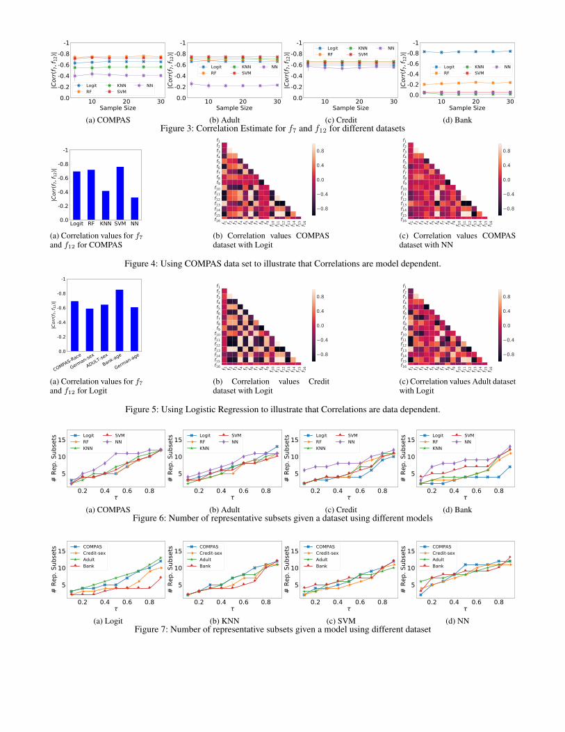
Bank marketing6: Published by (Moro, Cortez, and Rita2014) the data is related to direct marketing campaigns num-ber of phone calls of a Portuguese banking institution. Theclassification goal is to predict if a client will subscribe to aterm deposit (variable Y ). The Dataset contains 41188 and20 attributes that are collected from May 2008 to November2010. We consider age as the sensitive attribute.Performance EvaluationIn order to estimate between-fairness correlations using ourproposed Monte-Carlo method, we use 1000 sampled mod-els for each round and repeat the estimation process 30times. Our proposed approaches are evaluated using a set ofcommon classifiers; Logistic Regression (Logit), RandomForest (RF), K-nearest Neighbor (KNN) , Support VectorMachines (SVM) with linear kernel, and Neural Networks(NN) with one dense layer. Our findings are transferable toother classifiers.Correlation estimation quality: We begin our experimentsby evaluating the performance of our correlation estimationmethod. Recall that we designed Monte-carlo method. Inevery iteration, the algorithm uses the sampling oracle andsamples classifiers to evaluate correlations between pairs offairness notions, for which we use 1K samples. To see theimpact of number of estimation iteration in the estimationvariance and confidence error, we varied the number of it-erations from 2 to 30 times. Since the number of estimation
2https://aif360.readthedocs.io/en/latest/3ProPublica, https://bit.ly/35pzGFj4CI repository, https://bit.ly/2GTWz9Z5UCI repository, https://bit.ly/36x9t8o6UCI repository, https://archive.ics.uci.edu/ml/datasets/Bank+
Marketing
pairs are quadratic to |F|, we decided to (arbitrarily) picka par of notions and provide the results for it. To be con-sistent across the experiments, we fixed the pair f7 and f12for all data sets/models/settings. We confirm that the resultsand findings for other pairs of notions are consistent to whatpresented.7 Figure 3 provides the results for f7 and f12 forCOMPAS (a), Adult (b), Credit (c), Bank (d) datasets. Look-ing at the figure, one can confirm the stable estimation andsmall confidence error bars which demonstrate the high ac-curacy of our estimation. Also, as the number of iterationsincrease the estimation variance and confidence error signif-icantly decreases.Impact of data/model on correlation values: In this pa-per, we proposed to identify representative fairness metricsfor a given context (data and model). The underlying as-sumption behind this proposal is that correlations are dataand model dependent. Having evaluated our correlation es-timation quality, in this experiment we verify that the data/-model dependent assumptions for the correlations are valid.To do so, we first fix the data set to see if the correlationsare model dependent (Figure 4) and then fix the model tosee if the correlations are model dependent (Figure 5). First,we confirm that the results for other data sets/models areconsistent with what presented here. Looking at Figure 4, itis clear that correlations are model dependent. In particular,generally speaking, the complex boundary of the non-linearmodels (e.g. NN) reduce the correlation between fairnessmetrics, compared to linear models (e.g. Logit). Similarly,Figure 5 verifies that correlations are data dependent. Thisis because different data sets represent different underlyingdistributions with different properties impacting the fairnessvalues.Number of representative metrics: Next, we evaluate theimpact of the parameter parameter τ , used for identify-ing the representative metrics, in the number of represen-tatives RF . Figure 6 present the results for various valuesof the threshold τ for each ML model for COMPAS, Adult,Credit, Bank datasets. The thresholds values are selected asτ ∈ {0.1, 0.2, · · · , 0.9}. We can observe that as τ increasesthe number of subsets increases. For non-linear classifierssuch as NN, the number of subsets is relatively larger due tothe sensitivity of the non-linear decision boundaries to thesubset of samples in the training set. In such situation, thefairness metrics would be less correlated. In general, fair-ness metrics of linear decision boundaries are more corre-lated. Although similar overall pattern can be observed fromone dataset to another, the number of subset of representa-tives are different. The results indicates that the proposedapproach for estimation of correlation is model dependent.
In our next experiments, Figure 7, represents the numberof representative subsets of fairness metrics, RF , for differ-ent datasets fixing the ML model. We demonstrate that givena model as τ increases the size of RF increases. The non-linear models as expected, require more subsets The resultsindicates that the proposed approach for estimation of corre-lation is data dependent.
To provide an example of representative subsets of fair-
7Complimentary results are provided in the appendix.
10 20 30Sample Size
0.0-0.2-0.4-0.6-0.8
-1|C
orr(f
7,f 1
2)|
LogitRF
KNNSVM
NN
(a) COMPAS
10 20 30Sample Size
0.0-0.2-0.4-0.6-0.8
-1
|Cor
r(f7,
f 12)
|
LogitRF
KNNSVM
NN
(b) Adult
10 20 30Sample Size
0.0-0.2-0.4-0.6-0.8
-1
|Cor
r(f7,
f 12)
| LogitRF
KNNSVM
NN
(c) Credit
10 20 30Sample Size
0.0-0.2-0.4-0.6-0.8
-1
|Cor
r(f7,
f 12)
|
LogitRF
KNNSVM
NN
(d) BankFigure 3: Correlation Estimate for f7 and f12 for different datasets
Logit RF KNN SVM NN0.0
-0.2
-0.4
-0.6
-0.8
-1
|Cor
r(f7,
f 12)
|
(a) Correlation values for f7and f12 for COMPAS
f 1 f 2 f 3 f 4 f 5 f 6 f 7 f 8 f 9 f 10
f 11
f 12
f 13
f 14
f 15
f 16
f1f2f3f4f5f6f7f8f9
f10f11f12f13f14f15f16
0.8
0.4
0.0
0.4
0.8
(b) Correlation values COMPASdataset with Logit
f 1 f 2 f 3 f 4 f 5 f 6 f 7 f 8 f 9 f 10
f 11
f 12
f 13
f 14
f 15
f 16
f1f2f3f4f5f6f7f8f9
f10f11f12f13f14f15f16
0.8
0.4
0.0
0.4
0.8
(c) Correlation values COMPASdataset with NN
Figure 4: Using COMPAS data set to illustrate that Correlations are model dependent.
COMPAS-Race
German-sex
ADULT-sexBank-age
German-age0.0
-0.2
-0.4
-0.6
-0.8
-1
|Cor
r(f7,
f 12)
|
(a) Correlation values for f7and f12 for Logit
f 1 f 2 f 3 f 4 f 5 f 6 f 7 f 8 f 9 f 10
f 11
f 12
f 13
f 14
f 15
f 16
f1f2f3f4f5f6f7f8f9
f10f11f12f13f14f15f16
0.8
0.4
0.0
0.4
0.8
(b) Correlation values Creditdataset with Logit
f 1 f 2 f 3 f 4 f 5 f 6 f 7 f 8 f 9 f 10
f 11
f 12
f 13
f 14
f 15
f 16
f1f2f3f4f5f6f7f8f9
f10f11f12f13f14f15f16
0.8
0.4
0.0
0.4
0.8
(c) Correlation values Adult datasetwith Logit
Figure 5: Using Logistic Regression to illustrate that Correlations are data dependent.
0.2 0.4 0.6 0.8
5
10
15
# Re
p. S
ubse
ts LogitRFKNN
SVMNN
(a) COMPAS
0.2 0.4 0.6 0.8
5
10
15
# Re
p. S
ubse
ts LogitRFKNN
SVMNN
(b) Adult
0.2 0.4 0.6 0.8
5
10
15
# Re
p. S
ubse
ts LogitRFKNN
SVMNN
(c) Credit
0.2 0.4 0.6 0.8
5
10
15
# Re
p. S
ubse
ts LogitRFKNN
SVMNN
(d) BankFigure 6: Number of representative subsets given a dataset using different models
0.2 0.4 0.6 0.8
5
10
15
# Re
p. S
ubse
ts COMPASCredit-sexAdultBank
(a) Logit
0.2 0.4 0.6 0.8
5
10
15
# Re
p. S
ubse
ts COMPASCredit-sexAdultBank
(b) KNN
0.2 0.4 0.6 0.8
5
10
15
# Re
p. S
ubse
ts COMPASCredit-sexAdultBank
(c) SVM
0.2 0.4 0.6 0.8
5
10
15
# Re
p. S
ubse
ts COMPASCredit-sexAdultBank
(d) NNFigure 7: Number of representative subsets given a model using different dataset

FPR_rat
abs_odd_dif
dis_rat
DI
FNR_dif
PP
odd_dif
Pred_Eq
SP
E_Opp
FNR_raterr_rat
err_dif
dis_dif
FOR_dif
FOR_rat
(a) COMPAS-Logit
err_diferr_rat
DI
FPR_rat
odd_dif
Pred_EqSP E_Opp
FNR_rat
FOR_rat dis_dif
FOR_dif
FNR_dif
PP
dis_rat
abs_odd_dif
(b) COMPAS-NNFigure 8: Graph illustration of identified subset of fairness representatives–COMPAS
E_Opp
dis_dif
Pred_Eq
FOR_rat
SP
FNR_rat
odd_dif
dis_rat
err_dif
err_ratFPR_rat
FOR_dif
DI
FNR_dif
abs_odd_dif
PP
(a) Credit-Logit
dis_rat
PP
Pred_Eq
dis_difSP
E_Opp
odd_dif
err_dif
err_ratFPR_rat
DI
FOR_rat
abs_odd_difFOR_dif
FNR_rat
FNR_dif
(b) Credit-NNFigure 9: Graph illustration of identified subset of fairness representatives–Credit
ness metrics, Figure 8, we illustrate a graph with nodes rep-resenting the fairness metrics, orange nodes indicating therepresentative metrics of each subset, and edges showingthe subsets of metrics that are highly correlated. We usedτ = 0.5 for this plot. The graph confirms that the number ofsubsets are smaller using Logit model than that using NN,as previously discussed. Similarly, Figure 9 shows the rep-resentative metrics for Credit dataset using Logit and NNmodels. Discovery Ratio, Predictive Parity, Equality of Op-portunity, and Average Odd Difference are selected as repre-sentative metrics for Credit dataset when we use Logit clas-sifier.
Related workAlgorithmic fairness have been studied extensively in recentyears (Corbett-Davies et al. 2017; Kleinberg et al. 2018).Various fairness metrics have been defined in the literature toaddress the inequalities of the algorithmic decision makingfrom different perspectives. (Barocas, Hardt, and Narayanan2017) and (Verma and Rubin 2018) define different fairnessnotions in details. Majority of works focus on the fairnessconsideration in different stages of predictive modeling in-cluding pre-processing (Feldman et al. 2015; Kamiran andCalders 2012; Calmon et al. 2017), in-processing (Caldersand Verwer 2010; Zafar et al. 2015; Asudeh et al. 2019),and post-processing (Pleiss et al. 2017; Feldman et al. 2015;Stoyanovich, Yang, and Jagadish 2018; Hardt, Price, andSrebro 2016) to mitigate bias of the outcome. Furthermore,the proposed interventions are tied to a specific notion offairness; statistical parity (Calders and Verwer 2010), equal-ity of opportunity (Hardt, Price, and Srebro 2016), disparate
impact (Feldman et al. 2015), etc. A few recent work, dis-cuss the challenge of choosing the appropriate fairness met-ric for bias mitigation considerations. (Makhlouf, Zhioua,and Palamidessi 2021) surveys notions of fairness and dis-cusses the subjectivity of different notions for a set of real-world scenarios. The challenges about a growing pool offairness metrics for unfairness mitigation and some aspectsof the relationships between fairness metrics are highlightedin (Castelnovo et al. 2021) with respect to the distinctions in-dividual vs. group and observational vs. causality-based. Asa result, the authors highly promotes quantitative researchfor fairness metric assessment for bias mitigation. Buildingon previous works (Kleinberg, Mullainathan, and Raghavan2016; Chouldechova 2017), (Garg, Villasenor, and Foggo2020) provides a comparative using mathematical represen-tations to discuss the trade-off between some of the commonnotions of fairness.
Final Remarks
The abundance, trade-offs, and details of fairness metricsis a major challenge towards responsible practices of ma-chine learning for the ordinary data scientists. To alleviatethe overwhelming task of selecting a subset of fairness mea-sures to consider for a context (a data set and a model type),we proposed a framework that, given a set of fairness no-tions of interest, estimates the correlations between them andidentifies a subset of notions that represent others. Our com-prehensive experiments on benchmark data sets and differ-ent classification models verify the validity of out proposaland effectiveness of our approach.

ReferencesAgarwal, A.; Beygelzimer, A.; Dudık, M.; Langford, J.; andWallach, H. 2018. A reductions approach to fair classifica-tion. In ICML, 60–69.Angwin, J.; Larson, J.; Mattu, S.; and Kirchner, L. 2016.Machine Bias: Risk Assessments in Criminal Sentencing.ProPublica.Asudeh, A.; Jagadish, H.; Stoyanovich, J.; and Das, G. 2019.Designing Fair Ranking Schemes. In SIGMOD. ACM.Bansal, N.; Blum, A.; and Chawla, S. 2004. Correlationclustering. Machine learning, 56(1): 89–113.Barocas, S.; Hardt, M.; and Narayanan, A. 2017. Fairness inmachine learning. Nips tutorial, 1: 2017.Bellamy, R. K. E.; Dey, K.; Hind, M.; Hoffman, S. C.;Houde, S.; Kannan, K.; Lohia, P.; Martino, J.; Mehta, S.;Mojsilovic, A.; Nagar, S.; Ramamurthy, K. N.; Richards,J.; Saha, D.; Sattigeri, P.; Singh, M.; Varshney, K. R.; andZhang, Y. 2018. AI Fairness 360: An Extensible Toolkit forDetecting, Understanding, and Mitigating Unwanted Algo-rithmic Bias.Calders, T.; and Verwer, S. 2010. Three naive Bayes ap-proaches for discrimination-free classification. Data Miningand Knowledge Discovery, 21(2): 277–292.Calmon, F.; Wei, D.; Vinzamuri, B.; Ramamurthy, K. N.;and Varshney, K. R. 2017. Optimized pre-processing for dis-crimination prevention. In Advances in Neural InformationProcessing Systems, 3992–4001.Castelnovo, A.; Crupi, R.; Greco, G.; and Regoli, D. 2021.The zoo of Fairness metrics in Machine Learning. arXivpreprint arXiv:2106.00467.Celis, L. E.; Huang, L.; Keswani, V.; and Vishnoi, N. K.2019. Classification with fairness constraints: A meta-algorithm with provable guarantees. In Proceedings of theconference on fairness, accountability, and transparency,319–328.Chouldechova, A. 2017. Fair prediction with disparate im-pact: A study of bias in recidivism prediction instruments.Big data, 5(2): 153–163.Corbett-Davies, S.; Pierson, E.; Feller, A.; Goel, S.; andHuq, A. 2017. Algorithmic decision making and the costof fairness. In Proceedings of the 23rd acm sigkdd interna-tional conference on knowledge discovery and data mining,797–806.Durrett, R. 2010. Probability: theory and examples. Cam-bridge university press.Efron, B.; and Tibshirani, R. J. 1994. An introduction to thebootstrap. CRC press.Feldman, M.; Friedler, S. A.; Moeller, J.; Scheidegger, C.;and Venkatasubramanian, S. 2015. Certifying and removingdisparate impact. In SIGKDD, 259–268. ACM.Friedler, S. A.; Scheidegger, C.; Venkatasubramanian, S.;Choudhary, S.; Hamilton, E. P.; and Roth, D. 2019. A com-parative study of fairness-enhancing interventions in ma-chine learning. In FAT*.
Garg, P.; Villasenor, J.; and Foggo, V. 2020. Fairness met-rics: A comparative analysis. In Big Data, 3662–3666.IEEE.Hardt, M.; Price, E.; and Srebro, N. 2016. Equality of op-portunity in supervised learning. Advances in neural infor-mation processing systems, 29: 3315–3323.Hesterberg, T. 2011. Bootstrap. Wiley Interdisciplinary Re-views: Computational Statistics, 3(6): 497–526.Hickernell, F. J.; Jiang, L.; Liu, Y.; and Owen, A. B. 2013.Guaranteed conservative fixed width confidence intervalsvia Monte Carlo sampling. In Monte Carlo and Quasi-Monte Carlo Methods 2012, 105–128. Springer.Kamiran, F.; and Calders, T. 2012. Data preprocessing tech-niques for classification without discrimination. Knowledgeand Information Systems, 33(1): 1–33.Kamiran, F.; Calders, T.; and Pechenizkiy, M. 2010. Dis-crimination aware decision tree learning. In ICDM, 869–874. IEEE.Kim, J. S.; Chen, J.; and Talwalkar, A. 2020. Fact: A diag-nostic for group fairness trade-offs. In ICML, 5264–5274.PMLR.Kleinberg, J.; Ludwig, J.; Mullainathan, S.; and Rambachan,A. 2018. Algorithmic fairness. In Aea papers and proceed-ings, volume 108, 22–27.Kleinberg, J.; Mullainathan, S.; and Raghavan, M. 2016.Inherent trade-offs in the fair determination of risk scores.arXiv preprint arXiv:1609.05807.Makhlouf, K.; Zhioua, S.; and Palamidessi, C. 2021. Onthe applicability of machine learning fairness notions. ACMSIGKDD Explorations Newsletter, 23(1): 14–23.Moro, S.; Cortez, P.; and Rita, P. 2014. A data-driven ap-proach to predict the success of bank telemarketing. Deci-sion Support Systems, 62: 22–31.Narayanan, A. 2018. Translation tutorial: 21 fairness defi-nitions and their politics. In Proc. Conf. Fairness Account-ability Transp., New York, USA, volume 1170.Neter, J.; Kutner, M. H.; Nachtsheim, C. J.; Wasserman, W.;et al. 1996. Applied linear statistical models.Pleiss, G.; Raghavan, M.; Wu, F.; Kleinberg, J.; and Wein-berger, K. Q. 2017. On fairness and calibration. In Advancesin Neural Information Processing Systems, 5680–5689.Robert, C. P. 2004. Monte carlo methods. Wiley OnlineLibrary.Stoyanovich, J.; Yang, K.; and Jagadish, H. 2018. Online SetSelection with Fairness and Diversity Constraints. In EDBT.Verma, S.; and Rubin, J. 2018. Fairness definitions ex-plained. In 2018 ieee/acm international workshop on soft-ware fairness (fairware), 1–7. IEEE.Zafar, M. B.; Valera, I.; Rodriguez, M. G.; and Gummadi,K. P. 2015. Fairness constraints: Mechanisms for fair classi-fication. arXiv preprint arXiv:1507.05259.Zhang, H.; Chu, X.; Asudeh, A.; and Navathe, S. B. 2021.OmniFair: A Declarative System for Model-Agnostic GroupFairness in Machine Learning. In SIGMOD, 2076–2088.

Pseudocodes
Algorithm 1: CorrEstimate
Input: Data set D, Fairness notions of interest F = {f1 · · · fm}Output: O, target data set1: for `← 1 to L do // number of iterations2: (T ,test-set)←split(D)// T is training set3: 〈G0,G1,G2,G3〉 ← 〈T [S = 0, Y = 0], T [S = 0, Y =
1], T [S = 1, Y = 0], T [S = 1, Y = 1]〉4: F ← [] // Table of fairness values5: for i← 1 to n do6: Fi1 · · ·Fim ←SamplingOracle(〈G0,G1,G2,G3〉,F)7: corr` ←corr(F ) // Pearson correlations
8: for i, j ← 1 to m do9: corr[i, j]←avg(corr1[i, j] · · · corrL[i, j])
10: e[i, j]← Z(1, α2) stdev(corr1[i, j] · · · corrK [i, j])/
√L
11: return (corr, e)
Algorithm 2: SamplingOracle
Input: 〈G0,G1,Gr,G3〉,F , model-type, t-sizeOutput: F1 · · ·Fm1: for i← 1 to r do2: wi ← uniform(0, 1)// random uniform in
range [0,1]3: w1 · · ·wr ← w1
|w| · · ·wr|w| // normalize
4: t-set← [] // training set5: for i = 1 to r do6: for j = 1 to wi×t-size do7: rand-index←random(1, |Gi|)8: add Gi[rand-index] to t-set9: model←train(t-set, model-type)
10: for i = 1 to m do11: Fi ←audit(model, fi)12: return F1 · · ·Fm
Complimentary Experiment ResultsFigure 10 (a) and (b) show similar results for the correla-tion estimates, using Credit dataset with S=age referred toas ”Credit-age”.
Figures 11 and 12 demonstrate a comprehensive compar-ison on the number of representative subsets between differ-ent models using all of datasets (including credit-age). Aswe can observer and discussed before, the number of repre-sentative subsets are model-dependent.
Figure 13 illustrate the correlation estimations for Credit-age dataset. Note that in (c) the correlation estimates forcertain pairs are missing, when we use NN. The reason formissing correlations is the NA values for f9 which indicatethat FN1 is zero for this case. Similarly for f14, since FN1
is zero it yiels NA for FNR ratio which is f14. In addition,f8 is always zero for any sampled model (FOR disparity rateis zero). Similarly for f13 the disparity is zero.
10 20 30Sample Size
0.0-0.2-0.4-0.6-0.8
-1
|Cor
r(f7,
f 12)
| LogitRF
KNNSVM
NN
(a) Correlation Estimate for f7 and f12 for Credit-age
0.2 0.4 0.6 0.8
5
10
15
# Re
p. S
ubse
ts LogitRFKNN
SVMNN
(b) Number of representative subsets for Credit-age
Figure 10: Results for Credit-age dataset

0.2 0.4 0.6 0.8
5
10
15
# Re
p. S
ubse
ts COMPASCredit-sexAdultBankCredit-age
(a) Logit
0.2 0.4 0.6 0.8
5
10
15
# Re
p. S
ubse
ts COMPASCredit-sexAdultBankCredit-age
(b) RF
0.2 0.4 0.6 0.8
5
10
15
# Re
p. S
ubse
ts COMPASCredit-sexAdultBankCredit-age
(c) KNN
Figure 11: Number of representative subsets given a model using different datasets (Logit, RF, KNN)
0.2 0.4 0.6 0.8
5
10
15
# Re
p. S
ubse
ts COMPASCredit-sexAdultBankCredit-age
(a) SVM
0.2 0.4 0.6 0.8
5
10
15#
Rep.
Sub
sets COMPAS
Credit-sexAdultBankCredit-age
(b) NN
Figure 12: Number of representative subsets given a model using different datasets (SVM, NN)
Logit RF KNN SVM NN0.0
-0.2
-0.4
-0.6
-0.8
-1
|Cor
r(f7,
f 12)
|
(a) Correlation values for f7and f12 for Credit-age
f 1 f 2 f 3 f 4 f 5 f 6 f 7 f 8 f 9 f 10
f 11
f 12
f 13
f 14
f 15
f 16
f1f2f3f4f5f6f7f8f9
f10f11f12f13f14f15f16
0.8
0.4
0.0
0.4
0.8
(b) Correlation values Credit-agedataset with Logit
f 1 f 2 f 3 f 4 f 5 f 6 f 7 f 8 f 9 f 10
f 11
f 12
f 13
f 14
f 15
f 16
f1f2f3f4f5f6f7f8f9
f10f11f12f13f14f15f16
0.8
0.4
0.0
0.4
0.8
(c) Correlation values Credit-agedataset with NN
Figure 13: Using Credit-age data set to illustrate that Correlations are model dependent.

E_Opp
dis_dif
Pred_Eq
FOR_rat
SP
FNR_rat
odd_dif
dis_rat
err_dif
err_ratFPR_rat
FOR_dif
DI
FNR_dif
abs_odd_dif
PP
(a) Credit-age5
PP
dis_rat
err_dif
err_ratFPR_rat
DI E_Opp
Pred_Eq
SP
odd_dif
dis_difabs_odd_dif
FOR_rat
FOR_difFNR_rat
FNR_dif
(b) Credit-age-NNFigure 14: Graph illustration of identified subset of fairness representatives–Credit-age
Logit RF KNN SVM NN0.0
-0.2
-0.4
-0.6
-0.8
-1
|Cor
r(f6,
f 7)|
(a) Correlation values for f6 and f7for Logit
Logit RF KNN SVM NN0.0
-0.2
-0.4
-0.6
-0.8
-1
|Cor
r(f2,
f 8)|
(b) Correlation values for f2 and f8for Logit
Logit RF KNN SVM NN0.0
-0.2
-0.4
-0.6
-0.8
-1
|Cor
r(f10
,f12
)|
(c) Correlation values for f11 andf13 for Logit
Logit RF KNN SVM NN0.0
-0.2
-0.4
-0.6
-0.8
-1
|Cor
r(f4,
f 15)
|
(d) Correlation values for f5 andf16 for Logit
Figure 15: Correlation Estimates for different pairs on COMPAS dataset using different models.
Logit RF KNN SVM NN0.0
-0.2
-0.4
-0.6
-0.8
-1
|Cor
r(f7,
f 12)
|
(a) Correlation values for f7and f12 for Bank
f 1 f 2 f 3 f 4 f 5 f 6 f 7 f 8 f 9 f 10
f 11
f 12
f 13
f 14
f 15
f 16
f1f2f3f4f5f6f7f8f9
f10f11f12f13f14f15f16
0.8
0.4
0.0
0.4
0.8
(b) Correlation values Bank datasetwith Logit
f 1 f 2 f 3 f 4 f 5 f 6 f 7 f 8 f 9 f 10
f 11
f 12
f 13
f 14
f 15
f 16
f1f2f3f4f5f6f7f8f9
f10f11f12f13f14f15f16
0.8
0.4
0.0
0.4
0.8
(c) Correlation values Credit-agedataset with NN
Figure 16: Using Bank data set to illustrate that Correlations are model dependent.
f 1 f 2 f 3 f 4 f 5 f 6 f 7 f 8 f 9 f 10
f 11
f 12
f 13
f 14
f 15
f 16
f1f2f3f4f5f6f7f8f9
f10f11f12f13f14f15f16
0.8
0.4
0.0
0.4
0.8
(a) Correlation values Bank datasetwith RF
f 1 f 2 f 3 f 4 f 5 f 6 f 7 f 8 f 9 f 10
f 11
f 12
f 13
f 14
f 15
f 16
f1f2f3f4f5f6f7f8f9
f10f11f12f13f14f15f16
0.8
0.4
0.0
0.4
0.8
(b) Correlation values Bank datasetwith KNN
f 1 f 2 f 3 f 4 f 5 f 6 f 7 f 8 f 9 f 10
f 11
f 12
f 13
f 14
f 15
f 16
f1f2f3f4f5f6f7f8f9
f10f11f12f13f14f15f16
0.8
0.4
0.0
0.4
0.8
(c) Correlation values Bank datasetwith SVM
Figure 17: Using Bank dataset to illustrate that Correlations are model dependent.