representation of a smooth isometric deformation of a · pdf filerepresentation of a smooth...
TRANSCRIPT

J Elast (2018) 130:145–195DOI 10.1007/s10659-017-9637-2
Representation of a Smooth Isometric Deformationof a Planar Material Region into a Curved Surface
Yi-Chao Chen1 · Roger Fosdick2 · Eliot Fried3
Received: 7 January 2017 / Published online: 10 April 2017© The Author(s) 2017. This article is published with open access at Springerlink.com
Abstract We consider the problem of characterizing the smooth, isometric deformationsof a planar material region identified with an open, connected subset D of two-dimensionalEuclidean point space E
2 into a surface S in three-dimensional Euclidean point space E3.
To be isometric, such a deformation must preserve the length of every possible arc of ma-terial points on D. Characterizing the curves of zero principal curvature of S is of majorimportance. After establishing this characterization, we introduce a special curvilinear co-ordinate system in E
2, based upon an à priori chosen pre-image form of the curves of zeroprincipal curvature in D, and use that coordinate system to construct the most general iso-metric deformation of D to a smooth surface S. A necessary and sufficient condition for thedeformation to be isometric is noted and alternative representations are given. Expressionsfor the curvature tensor and potentially nonvanishing principal curvature of S are derived.A general cylindrical deformation is developed and two examples of circular cylindrical andspiral cylindrical form are constructed. A strategy for determining any smooth isometricdeformation is outlined and that strategy is employed to determine the general isometric de-formation of a rectangular material strip to a ribbon on a conical surface. Finally, it is shownthat the representation established here is equivalent to an alternative previously establishedby Chen, Fosdick and Fried (J. Elast. 119:335–350, 2015).
Mathematics Subject Classification 53A05 · 74K15 · 74K35 · 57R40 · 53A45
B E. [email protected]
Y.-C. [email protected]
1 Department of Mechanical Engineering, University of Houston, Houston, TX 77204-4006, USA
2 Department of Aerospace Engineering and Mechanics, University of Minnesota, Minneapolis,MN 55455-0153, USA
3 Mathematical Soft Matter Unit, Okinawa Institute of Science and Technology Graduate University,Okinawa 904-0495, Japan
146 Y.-C. Chen et al.
Keywords Isometry · Unstretchable · Inextensional · Ruled · Developable · Embedding
Contents
1 Introduction . . . . . . . . . . . . . . . . . . . . . . . . . . . . . . . . . . . . . . . 1462 Notion of an Isometric Deformation . . . . . . . . . . . . . . . . . . . . . . . . . 1483 General Analysis and Set-up: Isometric Deformation of D ⊂ E
2 to S ⊂ E3 . . . . 151
4 Coordinate Representation of an Isometric Deformation: Necessary andSufficient Condition . . . . . . . . . . . . . . . . . . . . . . . . . . . . . . . . . . 156
5 Alternative Representative Forms of an Isometric Deformation . . . . . . . . . . 1596 Curvature Tensor of S . . . . . . . . . . . . . . . . . . . . . . . . . . . . . . . . . 1627 General Cylindrical Bending . . . . . . . . . . . . . . . . . . . . . . . . . . . . . 164
7.1 Example 1: Circular Cylindrical Bending. Helical Forms . . . . . . . . . . . 1667.2 Example 2: Spiral Cylindrical Bending. Helical Forms . . . . . . . . . . . . 167
8 Summary: Strategy for Determining an Isometric Deformation of D ⊂ E2 to
S ⊂ E3 . . . . . . . . . . . . . . . . . . . . . . . . . . . . . . . . . . . . . . . . . 170
9 Isometric Deformation of a Rectangular Material Strip D ⊂ E2 to Portion S of a
Conical Surface K ⊂ E3 . . . . . . . . . . . . . . . . . . . . . . . . . . . . . . . . 172
9.1 General Case . . . . . . . . . . . . . . . . . . . . . . . . . . . . . . . . . . . 1739.2 Particular Example . . . . . . . . . . . . . . . . . . . . . . . . . . . . . . . . 181
10 Orthogonal Coordinate Representation of an Isometric Deformation: Necessaryand Sufficient Form . . . . . . . . . . . . . . . . . . . . . . . . . . . . . . . . . . 18210.1 The Isometric Deformation y in Terms of the Curve C ∈ S and Its
Coordinate Pre-image Curve C0 ∈ D . . . . . . . . . . . . . . . . . . . . . . 18610.2 Recovery of the Component y, or Its Equivalent y, of the Parametric
Representation of an Isometric Deformation y . . . . . . . . . . . . . . . . 19010.3 Curvature Tensor of S . . . . . . . . . . . . . . . . . . . . . . . . . . . . . . 192
11 Discussion . . . . . . . . . . . . . . . . . . . . . . . . . . . . . . . . . . . . . . . 193Acknowledgements . . . . . . . . . . . . . . . . . . . . . . . . . . . . . . . . . . . . 195References . . . . . . . . . . . . . . . . . . . . . . . . . . . . . . . . . . . . . . . . . 195
1 Introduction
Recently, we [1] established an explicit necessary and sufficient representation for a three-times continuously differentiable, isometric deformation of a planar material region identi-fied with an open, connected region D in two-dimensional Euclidean point space E
2 into asurface S in three-dimensional Euclidean point space E
3. Each such deformation is deter-mined by a sufficiently smooth space curve C, the directrix, and a family of straight lines,the generators. A condition necessary, but not sufficient, for the deformation to be isometricis that the generator at each point of C lies in the plane orthogonal to C at that point, withits precise orientation within that plane being determined by the cumulative torsion of C.Additionally, however, each ordered combination (u, v) of arclength u along the directrixand distance v along the generators must correspond isometrically to a unique material pointx in D. That correspondence takes the form of an implicit relation, involving convoluted de-pendence on the curvature and torsion of C, and admits a closed-form solution only in verysimple examples, encountered for instance in the construction of the isometric deformationthat bends a half disk into a conical surface.

Isometric Deformation of a Planar Material Region into a Curved. . . 147
In the present paper, we describe an alternative strategy designed to mitigate the afore-mentioned difficulties. This strategy produces a different, but equivalent, necessary and suf-ficient representation for the class of isometric deformations of planar material regions andit corrects a fundamental misunderstanding concerning an interpretation of the coordinaterepresentation that has circulated in the mainstream literature on the subject. We consideronly kinematical issues, leaving questions surrounding the variational characterization ofequilibrium configurations for future consideration.
Our primary objective is to determine a representation for the most general smooth iso-metric deformation y that takes each point x in an open, connected subset D of E2 to a pointy on a surface S in E
3:
y = y(x). (1.1)
Our approach hinges on a characterization, provided in Sect. 3, of the generators of anysurface S determined by such a deformation. This characterization leads naturally to theintroduction, in Sect. 4, of curvilinear coordinates (η1, η2) for D that correspond to an àpriori chosen form for the pre-images of the generators. Relative to a fixed orthonormalbasis {ı1, ı2} for the translation space V
2 of E2, each generator of S is the rotated and
translated ‘rigid image’ of a straight line in D with orientation
b2(η1
) = cos θ(η1
)ı1 + sin θ
(η1
)ı2, (1.2)
where θ(η1) is the angle that the η2-coordinate line passing through the point x = η1ı1
makes with a line parallel to ı1. The (η1, η2)-coordinate system is of central importance toour construction. In particular, defining a parametrization y that maps D to S , but dependson position in D through the curvilinear coordinates (η1, η2), by
y(η1, η2
) = y(η1ı1 + η2b2
(η1
)), (1.3)
we establish the representation
y = y(η1, η2
) = y0
(η1
) + η2Q(η1
)b2
(η1
), (1.4)
where y0—which is defined such that y0(η1) = y(η1ı1) parametrizes the image of the
η2 = 0 coordinate line, namely the directrix C of S—is determined by integrating ˙y0 = Qı1
with y0(0) prescribed, where a superposed dot denotes differentiation with respect to η1,and Q(η1) is an element of the collection Orth+ of proper orthogonal linear transformationsfrom V
3, the translation space of E3, into itself. We then prove that the condition
Qb2 = 0 (1.5)
is both necessary and sufficient to ensure that y defined via (1.3)–(1.4) in conjunction witha ruled parametrization of D in terms of the curvilinear coordinates (η1, η2) is an isometricdeformation. The representation (1.4) for the component y of the isometric deformation y
admits various alternative forms described in Sect. 5. Suppose, in particular, that the directrixparametrized by y0 has nonvanishing curvature κ and, thus, possesses a well-defined Frenetframe with unit tangent t = ˙y0, unit binormal b, and torsion τ . The mapping y can then beexpressed as
y(η1, η2
) = y0
(η1
) + η2 sin θ(η1
)(
sgn(λ(η1
))b(η1
) + τ(η1)
κ(η1)t(η1
))
, (1.6)

148 Y.-C. Chen et al.
where λ is a scalar field related to the curvature and orientation of S and satisfies
|λ| = ∣∣ax
(QQ�)∣∣, (1.7)
with ax(QQ�) being the axial vector of the skew linear transformation QQ�. If, without re-gard for the overall consequences that are considered in Sect. 5, we naively set θ(η1) ≡ π/2,so that the generators of S must be orthogonal to its directrix, and additionally stipulate thatλ > 0, then the right-hand side of (1.6) can be recognized as the parametric form of the recti-fying developable of the directrix parametrized by y0. Hangan [3], Sabitov [4], Starostin andvan der Heijden [2], Kurono and Umehara [5], Chubelaschwili and Pinkall [6], Naokawa [7],Kirby and Fried [8], Shen et al. [9], and others have used rectifying developable mappingsto describe nominally isometric deformations of planar rectangular material material stripsinto ribbons and Möbius bands. These workers do not explain how to identify material pointsin the reference rectangle with the curvilinear coordinates (η1, η2). Nor do they provide acondition such as (1.5) which ensures that the parametric representation of the underlyingdeformation is indeed isometric to the extent that it preserves the length of every possiblearc of material points on the reference retangle. Importantly, these omissions undermine adimensional reduction argument that is used to ostensibly obtain the bending energy of arectangular strip that is isometrically deformed into a curved ribbon in terms of an integralover its midline. Moreover, they lead to variational strategies that involve comparing theenergies of differently shaped, generally nonrectangular, planar reference regions that aremapped, with stretching, into developable surfaces instead of with the isometric deforma-tions of a single rectangular material strip that cannot withstand stretching. See, also, thediscussion of Chen and Fried [10].
Expressions for the curvature tensor and potentially nonvanishing principal curvature of ageneral smooth surface S determined by an isometric deformation of a rectangular materialstrip are derived on the basis of our representation in Sect. 6. In Sect. 7, we specialize ourresults to obtain the most general smooth isometric deformation of a planar material regionto a cylindrical form and provide two elementary examples involving isometric deforma-tions of rectangular material strips. A summary of our strategy for determining any smoothisometric deformation of a planar material region is provided in Sect. 8. This strategy is thenused, in Sect. 9, to determine the isometric deformation of a rectangular material strip to aconical form. Next, in Sect. 10, we show the equivalence of the representation given in our[1] previous work and that obtained here. In particular, that equivalence rests on workingwith orthogonal curvilinear coordinates (ζ 1, ζ 2). Finally, in Sect. 11, we briefly review theconceptual position we have taken in this work regarding the isometric mappings of planarmaterial regions. We contrast our position with a few other notable works that do not regardthe surfaces as material entities and, rather, apply the concept of isometry as it is defined indifferential geometry.
2 Notion of an Isometric Deformation
Consider a three times continuously differentiable, deformation y that maps each point x
in a planar material region identified with an open, connected subset D of two-dimensionalpoint space E
2 to a point
y = y(x) (2.1)

Isometric Deformation of a Planar Material Region into a Curved. . . 149
on a surface S in three-dimensional Euclidean point space E3. We say that such a deforma-
tion is isometric if in taking D to S it preserves the length of every possible arc of materialpoints on D. This is the case if and only if the gradient
F = ∇y (2.2)
of y on D, the values of which are linear mappings from the translation space V2 of E2 to
the translation space V3 of E3, preserves the lengths of vectors in V
2 in the sense that
|Fu| = |u| (2.3)
for each u ∈V2. On this basis, we see that
Fu · Fv = 1
2
(∣∣F (u + v)∣∣2 − |Fu|2 − |Fv|2)
= 1
2
(|u + v|2 − |u|2 − |v|2)
= u · v (2.4)
for all u ∈V2 and v ∈V
2. Equivalently, F must obey
F �F = I , (2.5)
where I denotes the identity linear transformation on V2. The requirement that (2.3) holds
for all u ∈ V2 is also sufficient for y to be an isometric deformation, as is the requirement
that the gradient F of y satisfies (2.5).It is important to distinguish between our notion of an isometric deformation and an al-
ternative notion that is encountered in differential geometry—a notion that has been appliednaively when dealing with deformations of two-dimensional bodies which cannot withstandstretching. Such bodies are referred to as “inextensional” in the classical theories of plates(see, for example, Simmonds and Libai [11, 12]) and shells (see, for example, Libai andSimmonds [13, 14]) but are often referred to as “inextensible” in recent works on ribbon-like forms.
In differential geometry, it is commonly understood that a mapping of a part D of asurface A ⊂ E
3 onto a part S of a surface B ⊂ E3 is isometric, or length-preserving, if
the length of any arc on S is the same as the length of the inverse image of the arc onD. If such a mapping exists, then the surfaces D and S are said to be isometric. In thedifferential geometric concept of isometry, the surfaces A and B are considered as givenand the objective is to determine conditions which ensure that a length-preserving mappingexists between the corresponding parts D ⊂ A and S ⊂ B. Statements to the effect that“isometric surfaces must have the same Gaussian curvature at corresponding points of sucha mapping” and “if the Gaussian curvatures of D and S are constant and equal to one anotherthen the surfaces are isometric” are commonplace.1 So also is the statement “correspondingcurves on isometric surfaces have the same geodesic curvature at corresponding points”.Furthermore, it is well-known that if D and S are developable then the Gaussian curvaturesof both are zero and thus, in particular, D and S are isometric to one another from thedifferential geometric point of view.
1See, for example, Kreyszig [15, p. 164].
150 Y.-C. Chen et al.
In the kinematics of continuous two-dimensional material bodies, as is the concern ofthis paper, it is commonly understood that a mapping considered as a deformation of agiven material surface D ⊂ E
3 into a surface S ⊂ E3 is isometric (i.e., length-preserving,
unstretchable, or inextensional), if the length of any arc of material points on D is the sameas the length of the image of this material arc on the surface S ⊂ E
3 under the deformation.Any such mapping is considered to be a deformation of the surface D ⊂ E
3, which is iden-tified as a given reference configuration, and the objective is to determine conditions on thedeformation necessary and sufficient to ensure that it is length-preserving. If, for example,the material surface D is planar and its mapping, considered as a deformation of D �→ S ,produces a developable image S , then the Gaussian curvatures of both D and S are zerobut the mapping is not necessarily an isometric deformation. To illustrate, D ⊂ E
2 could bean undistorted, rectangular material ribbon which is mapped to S ⊂ Tc, where Tc ⊂ E
3 isa circular cylindrical surface. In this case, both D and S have zero Gaussian curvature, butthe mapping need not be an isometric deformation because stretching of material filamentsmay have taken place. To be an isometric deformation, the developability of the referencesurface D and its target image S is not sufficient, as we show later in Sect. 4 of this paper.
The notions of isometry that arise in differential geometry and in the kinematics ofcontinuous two-dimensional material bodies are fundamentally different. Importantly, how-ever, only the second of these notions is relevant when studying the deformation of a two-dimensional body that cannot withstand stretching.
In the setting of differential geometry, the surfaces A and B in E3 are preconceived
and given a priori without regard for how one is obtained from the other, and the centralquestion concerns whether lengths measured on a part D ⊂ A can be made to correspond to(i.e., be equal to) lengths measured on a part S ⊂ B for any mapping in the collection of allmappings of D �→ S . When such a mapping exists then the surfaces D and correspondingS are said to be geometrically isometric. From this standpoint, no surface is consideredto be a two-dimensional continuous material region and no mapping is considered to bethe deformation of such a body. Suppose, for example, that A and B are planar surfacesin E
3. Then, it is clear that a square part D ⊂ A and a square part of equal size S ⊂ B areisometric in the differential geometric sense. However, from the standpoint of the kinematicsof two-dimensional continuous material regions, if D ⊂ A is considered to be an undistortedmaterial reference configuration and if S ⊂ B is a distorted (i.e., stretched) image of D,then no square parts of equal size in D and S , respectively, are related by an isometricdeformation.
If A and B are developable surfaces in E3, then in the differential geometric sense there
generally exists an isometric image S ⊂ B of a part D of A. But, in the kinematics oftwo-dimensional continuous material regions there need not exist an isometric deformationwhich maps the same part D ⊂ A to S ⊂ B. The differential geometric isometric image of Ddoes not necessarily represent a deformation of the relevant points of A into the part S ⊂ B.In general, it is simply an image or overlay that defines a region S on B in which lengthscan be measured in the same way that they were measured in D ⊂ A. From the standpointof the kinematics of two-dimensional continuous material region, if A is developable thenan isometric deformation of a part D ⊂ A in E
3 will produce a developable surface S whichhas the additional property that the length between material points on D and the length be-tween corresponding material points on S under the deformation mapping are equal. Fromthis point of view, the requirement that a deformation maps a developable surface to a de-velopable surface is necessary for the underlying mapping to be an isometric deformationbut it does not suffice to ensure that material lengths are preserved. Thus, when consideringthe characterization of the deformation (i.e., bending and twisting) of a rectangular material
Isometric Deformation of a Planar Material Region into a Curved. . . 151
ribbon under the constraint that material lengths cannot be changed—which, for example,is the common hypothesis in deforming a rectangular strip of paper into a Möbius band—deformations are the only physically relevant class of mappings.
3 General Analysis and Set-up: Isometric Deformation of D ⊂ E2 to
S ⊂ E3
Let {ı1, ı2} denote a fixed orthonormal basis in the translation space V2 of E2, let xi denote
the component of x relative to ıi , i = 1,2, so that x = xiıi ,2 and define ı3 := ı1 × ı2, so that{ı1, ı2, ı3} provides a fixed positively-oriented orthonormal basis for the translation spaceV
3 of E3. With a slight abuse of notation, we may then write y(x) = y(x1, x2) and define abasis {ei , e2} at each point y = y(x) of S by
ei
(y(x)
) := y,i (x) (3.1)
for each material point x of D. The base vectors e1(x) and e2(x) are of course tangent to Sat y. With reference to (2.4), the requirement that y is an isometric deformation may thenbe expressed as
ei · ej = ıi · ıj = δij . (3.2)
By differentiating we thus have
y,ik ·y,j +y,i ·y,jk = 0 (3.3)
along with two similar equations obtained by cyclically permuting the indicies {i, j, k}. Byadding two of these equations and subtracting the other we easily arrive at
y,i ·y,jk = 0. (3.4)
Now, on introducing the oriented unit vector normal
n := e1 × e2 (3.5)
to S , we infer from (3.4) that, for each x ∈ D,
y,ij (x) = Aij (x)n(y(x)
), Aij (x) = Aji(x). (3.6)
Observing that y,ijk = y,ikj by the assumed smoothness of the mapping y, we readilysee from (3.6) that
Aij ,k n + Aijn,k = Aik,j n + Aikn,j . (3.7)
Thus, because n,i is orthogonal to n, we find from (3.7) that
Aij ,k = Aik,j =⇒ Aij = ai,j , (3.8)
which, with the symmetry condition (3.6)2, yields
ai,j = aj ,i =⇒ aj = φ,i . (3.9)
2Throughout this work, Roman indicies range over {1,2}, with summation over twice repeated indices beingimplicit, and a subscripted comma denotes partial differentiation.
152 Y.-C. Chen et al.
This shows that at points where the mapping y is smooth we may introduce a scalar field φ
satisfying
φ,ij = Aij . (3.10)
Consequently, (3.6) becomes
y,ij (x) = φ,ij (x)n(y(x)
). (3.11)
Moreover, (3.7) reduces to
φ,ij n,k = φ,ik n,j , (3.12)
which is equivalent to
εjkφ,ij n,k = 0, (3.13)
where εij is the usual alternator symbol for E2. Thus,
εjkφ,ij n,k ·em = 0. (3.14)
Now, because n,k ·em = −n · em,k and because (3.1) and (3.11) imply that em,k = y,mk =φ,mk n, this last relation may be written as
εjkφ,ij φ,mk = 0. (3.15)
Recognizing that the expression on the left-hand side of the above relation is skew in theindices i and m, we have equivalently
εimεjkφ,ij φ,mk = 0, (3.16)
which gives
det(φ,ij ) := φ,11 φ,22 −φ,212 = 0. (3.17)
Now let us recall some elementary differential geometry. Consider a smooth curve
L0 = {x ∈ D : x = x(β) = xi (β)ıi ,0 < β < β∗
}(3.18)
in D. The image L of this curve in S is then given by
L = {y ∈ S : y = y(β),0 < β < β∗
}, (3.19)
with y(β) := y(x(β)) for 0 < β < β∗, and, because y is an isometric deformation, we seethat the natural tangent vector e to L given by
e(β) := dy(β)
dβ, 0 < β < β∗, (3.20)
satisfies∣∣e(β)
∣∣ =∣∣∣∣dx(β)
dβ
∣∣∣∣, 0 < β < β∗. (3.21)
Also, the arclength parameter s is common to both L0 and L, and we have
ds = |e|dβ. (3.22)

Isometric Deformation of a Planar Material Region into a Curved. . . 153
Clearly, σ := e/|e| is a unit tangent vector to L ⊂ S . Finally, we record for later use that thechain rule gives
e = dy
dβ= y,i
(x(β)
)dxi (β)
dβ= ei
(y(β)
)dxi (β)
dβ, (3.23)
from which it follows that
dxi (β)
dβ= e(β) · ei
(y(β)
), 0 < β < β∗. (3.24)
The Frenet formula for L may be written as
dσ
ds= κm, (3.25)
where κ and m denote the curvature of L and the unit normal of L, respectively. The normalcurvature of S at y in the direction of σ on L is thus given by
κm · n = dσ
ds· n = −σ · dn
ds= −σ · (gradsn)σ , (3.26)
where gradsn = (gradsn)� denotes the surface gradient of the unit normal field in S and itsnegative represents the “curvature tensor” of S .3
In passing, if we let L0 be, respectively, an x1 or an x2 coordinate line in D, and associate,alternatively, the orthonormal base vectors e1 or e2 with σ then, because ei · n = 0 we haveei ,j ·n + ei · n,j = 0 and similar to (3.26) we may write
ei ,j ·n = −ei · (gradsn)ej . (3.27)
Thus, because of (3.1) and (3.11) we have for an isometric deformation the special result
φ,ij (x) = −ei (y) · (gradsn(y))ej (y)|y=y(x) (3.28)
for all x in D, which implies that
gradsn(y)|y=y(x) = −φ,ij (x)ei
(y(x)
) ⊗ ej
(y(x)
). (3.29)
Now, if we couple (3.29) with (3.17) we may conclude that, for an isometric deformation y
with n given by (3.1) and (3.5),
det(gradsn) = 0 (3.30)
at all points of S where the mapping y is smooth. This, of course, implies that a principalcurvature of S must vanish at all such points.
Now, let us associate the curve L ⊂ S with a curve of zero principal curvature of S . Thatis, let us suppose the natural tangent vector e = dy/dβ is an eigenvector of gradsn on Lwith zero eigenvalue. Thus, along L we have
(gradsn)e = 0. (3.31)
3The linear transformation −gradsn is also called the “Weingarten mapping” or the “shape operator” and itssymmetry property is a fundamental theorem of differential geometry. The principal values of −gradsn arethe principal curvatures of S at y.

154 Y.-C. Chen et al.
Further, the chain rule gives
dei (y(β))
dβ= dyi (x(β))
dβ= y,ij
(x(β)
)dxj (β)
dβ, 0 < β < β∗, (3.32)
which, with (3.11), yields
dei (y(β))
dβ= φ,ij
(x(β)
)dxj (β)
dβn(y(β)
), 0 < β < β∗. (3.33)
But, (3.29) and (3.23) show that
e(β) · (gradsn(x))ei (x)|x=y(β) = −φ,ij
(x(β)
)dxj (β)
dβ, 0 < β < β∗, (3.34)
and so, using the symmetry of gradsn, we see that
dei (y(β))
dβ= −(
e(β) · (gradsn(x))ei (x)
)n(x)|x=y(β)
= −(ei (x) · (gradsn(x)
)e(β)
)n(x)|x=y(β) = 0 (3.35)
for 0 < β < β∗. This means that
ei = constant along L, (3.36)
wherever L is smooth. As a consequence, the unit normal field n is also constant along Lwherever L is smooth, from which we infer that if L is smooth then it must lie on a fixedplane and the space curve L must consequently be planar. Moreover, from (3.23), we have
dy(β)
dβ= ei
dxi (β)
dβ, 0 < β < β∗, (3.37)
where we emphasize that ei is constant along L. Thus, on integrating with respect to β wefind that, for smooth L,
y(β) = ei xi (β) + c, 0 < β < β∗, (3.38)
where c is a constant vector in V3. Finally, we observe that for smooth L there is an element
Q of the collection Orth+ of proper orthogonal linear transformations from V3 to V
3 suchthat ei = Qıi , i = 1,2, at each point on L. This then gives
n = e1 × e2 = Qı1 × Qı2 = Qı3 on S (3.39)
and
y(β) = Qx(β) + c, 0 < β < β∗, (3.40)
the latter of which shows that L ⊂ S is a rotated and translated “rigid image” of L0 ⊂ D.Since L is planar, then if it is straight in S its pre-image, L0, is straight in D and is of thesame length; if it is curved in S its pre-image, L0, being an exact copy in D, must havechord lengths that are equal to those of L for points which correspond under the isometricdeformation y. Moreover, because all points on a chord of L0 must lie in D and L is planar,
Isometric Deformation of a Planar Material Region into a Curved. . . 155
then due to the isometry of y all points on the corresponding chord of L must lie in S andbe governed by y. This shows that the plane region defined by the closure of the interior ofthe convex hull of the planar curve L must be part of S .
Now, if two smooth curves, L(1) ⊂ S and L(2) ⊂ S , of zero principal curvature of Sintersect then they intersect at a point on S where the (oriented) surface unit normal iseither uniquely defined or the (oriented) surface has multiple unit normals. If the surfacenormal is unique then, arguing as above using the fact that in general the unit normal ofS must be constant along both L(1) and L(2), we see that because of the common normalat the intersection point the two curves must then lie in a common plane and all points inthe closure of the interior of the convex hull of these two curves must lie in a commonplanar part of S . If the surface unit normal is not unique at the point of intersection thenit has at least the two unit surface normals that are constant and propagated along L(1) andL(2), respectively; in this case the point of intersection is a “non-regular point” of S . Weshall not allow such situations in this work and consider only smooth surfaces S consistingsolely of regular points. In this case, an elementary argument based on the conclusions justestablished shows that S is composed of only two categories of subregions:
• Strips of S each of which contains a single one-parameter family of straight lines thatdo not intersect in S but run through S . These families describe the bent regions of S inwhich only one principal curvature of S vanishes.
• Planar strips of S each of which are bounded by straight lines of zero principal curvatureof S that do not intersect in S . Clearly, all continuous curves in such regions are curvesof zero principal curvature of S .
Even for the class of surfaces containing only regular points, as noted in the second ofthe above bullet items there may be continuous, non-differentiable curves of zero principlecurvature of S that lie on S . However, in this case such curves must again lie in a commonplanar part of S and the closure of the interior of its convex hull must also be in S . Of course,on planar parts of S all curves are curves of zero principal curvature of S .
To determine the form of the isometric deformation y, we must go further than simplythe partial characterization (3.40). This requires the introduction of another parameter α,say, and a study of a one-parameter family L(α) of straight lines of zero principal curvaturein S with corresponding pre-image lines L0(α) in D. Having taken this step, we may thenreplace the form (3.40) by
y(α,β) = Q(α)x(α,β) + c(α), (3.41)
where c(α) is a constant vector in V3 and x(α, ·) is given by
x(α,β) = xi (α,β)ıi = x0(α) + βb(α), (3.42)
with x0(α) parametrizing a specified curve in D and b(α) a unit vector along the straightline L0(α). Alternatively, we may write (3.41) as
y(α,β) = βQ(α)b(α) + y0(α), (3.43)
where y0(α) := y(α,0) = y(x0(α)) is the image in S of the curve x0(α) in D. The remain-ing difficulty at this stage lies with guaranteeing that (3.43) is, indeed, an isometric mappingof D to S ⊂ E
3. Moreover, having achieved this, we must also transform from the parame-ters (α,β) to the coordinates (x1, x2) and use (3.43) to determine the deformation y in theform y = y(x1, x2).

156 Y.-C. Chen et al.
Fig. 1 Coordinates for x = xi ıi in terms of (η1, η2)
4 Coordinate Representation of an Isometric Deformation: Necessaryand Sufficient Condition
For convenience, let us introduce the curvilinear coordinates (η1, η2) := (α,β) in E2 and
define the transformation (x1, x2) ←→ (η1, η2) by
x = xiıi = xi
(η1, η2
)ıi = x
(η1, η2
), (4.1a)
where
x1 = x1
(η1, η2
) = η1 + η2 cos θ(η1
),
x2 = x2
(η1, η2
) = η2 sin θ(η1
).
}
(4.1b)
The η1-coordinate line is coincident with the x1-coordinate line at η2 = 0 and the η2-coordinate lines run along straight lines in D that correspond to pre-images of the straightlines of zero principal curvature in S . The η2-coordinate line passing through (η1,0) formsan angle θ(η1) ∈ (0,π) with the x1-axis as shown in Fig. 1.
Clearly, the η1-coordinate lines corresponding to η2 = constant are not straight unless θ
is constant, except for η2 = 0, which then corresponds to the x1-axis. The base vectors ofV
2 through each x ∈ D ⊂ E2 for the curvilinear system are given by
bi = ∂x
∂ηi= ∂xm
∂ηi
∂x
∂xm
= ∂xm
∂ηiım, i = 1,2, (4.2a)

Isometric Deformation of a Planar Material Region into a Curved. . . 157
so that
b1 = ∂x
∂η1= (
1 − η2θ sin θ)ı1 + (
η2θ cos θ)ı2,
b2 = ∂x
∂η2= cos θ ı1 + sin θ ı2,
⎫⎪⎪⎪⎬
⎪⎪⎪⎭
(4.2b)
where a superposed dot is used to denote differentiation with respect to η1 and the depen-dencies of b1, b2, and θ on η1 are suppressed for brevity. Note, from (4.2b), that |b2| = 1and that (4.1a) takes the explicit form
x = x(η1, η2
) = η1ı1 + η2b2
(η1
). (4.3)
To ensure that {b1,b2} is an acceptable basis for representing the points of D ⊂ E2, we
restrict θ and η2 so that
det(bi · bj ) := |b1|2|b2|2 − (b1 · b2)2 = (
sin θ − η2θ)2 = 0 (4.4)
on D.4
Now, setting α = η1, β = η2, b(α) = b2(η1), and Q(α) = Q(η1) in (3.43), defining a
mapping y of (η1, η2) to S such that
y(η1, η2
) := y(x(η1, η2
)), (4.5)
and writing y0 = y(·,0) for the parametrization of the image in S of the η2 = 0 coordinateline (i.e., the x1-axis) in D, we arrive at the representation
y = y(η1, η2
) = y0
(η1
) + η2Q(η1
)b2
(η1
). (4.6)
From here we easily see that
ai := ∂y
∂ηi= ∂xm
∂ηiy,m = ∂xm
∂ηiem, i = 1,2. (4.7)
Thus, because (4.2a) implies that
∂xm
∂ηi= bi · ım, i = 1,2, (4.8)
and, because ei = Qıi , i = 1,2, we obtain the relations
ai = (bi · ım)em = (em ⊗ ım)bi = (Qım ⊗ ım)bi = Qbi , i = 1,2, (4.9)
which yield |ai | = |bi | for i = 1,2. In particular, we see that a2 = Qb2 is a unit vector fieldwhich defines the straight lines of zero curvature in S that are associated with the straightlines given by b2 in D. Note that (4.6) implies that
a1 = ∂y
∂η1= ˙y0 + η2(Qb2 + Qb2), (4.10)
4We shall see in (6.12) that the restriction (4.4) is related to the possible unboundedness of the curvature of S .

158 Y.-C. Chen et al.
where
˙y0
(η1
) = ∂y(η1,0)
∂η1= a1
(η1,0
) = Q(η1
)b1
(η1,0
) = Q(η1
)ı1, (4.11)
and that from (4.2b) we have
η2b2 = b1 − ı1. (4.12)
Thus, recalling from (4.9) that a1 = Qb1 we see from (4.10) that Q must satisfy
Qb2 = 0, (4.13)
which is a necessary condition on how the proper orthogonal transformation field Q may bechosen so that the deformation y of D ⊂ E
2 to S ⊂ E3 defined implicitly through (4.3) and
(4.6) is isometric. It readily follows that (4.13) is equivalent to QQ�a2 = 0 which meansthat the “angular velocity” corresponding to Q, namely the axial vector ax(QQ�) of theskew linear transformation field QQ�, must be parallel to a2.5 There thus exist a scalar fieldλ and a skew linear transformation A with axial unit vector a2, both generally dependentonly on η1 but independent of η2, such that
ax(QQ�) = λa2 and QQ� = λA. (4.14)
Of course, |λ| = |ax(QQ�)|.The condition (4.13) or, equivalently, (4.14) is not only necessary for the deformation y
of D ⊂ E2 to S ⊂ E
3 defined implicitly through (4.3) and (4.6) to be isometric, but it is alsosufficient. To verify this assertion, we first observe from (4.6) that
∇y := ∂y
∂ηi⊗ bi = ( ˙y0 + η2(Qb2 + Qb2)
) ⊗ b1 + Qb2 ⊗ b2, (4.15)
where {b1,b2}, with
b1 := sin θ ı1 − cos θ ı2
sin θ − η2θand b2 := −η2θ cos θ ı1 + (1 − η2θ sin θ)ı2
sin θ − η2θ, (4.16)
is the basis of V2 dual to {b1,b2}. Next, we observe that (4.11) and (4.12) allow us to write
∇y = (Qı1 + η2Qb2 + Qb1 − Qı1
) ⊗ b1 + Qb2 ⊗ b2, (4.17)
and, because of (4.13), we arrive at
∇y = Qb1 ⊗ b1 + Qb2 ⊗ b2 = Q(b1 ⊗ b1 + b2 ⊗ b2), (4.18)
which is equivalent to
∇y = Q(ı1 ⊗ ı1 + ı2 ⊗ ı2). (4.19)
Thus, because Q ∈ Orth+,
(∇y)�∇y = (ı1 ⊗ ı1 + ı2 ⊗ ı2)Q�Q(ı1 ⊗ ı1 + ı2 ⊗ ı2) = ı1 ⊗ ı1 + ı2 ⊗ ı2, (4.20)
5In this regard, note that a2(η1) is the orientation of the line L(η1) of zero curvature in S which corresponds
to the line L0(η1) that passes through the x1-axis at (η1,0) with orientation b2(η1) in D.
Isometric Deformation of a Planar Material Region into a Curved. . . 159
and this ensures that the length between any two points in D is preserved under the defor-mation y of x ∈ D to y ∈ S provided (4.13) holds.
5 Alternative Representative Forms of an Isometric Deformation
Note, from (4.11), that the unit tangent vector to the space curve parametrized by y0 is givenby
t := ˙y0 = Qı1 = e1, (5.1)
and, granted that t = 0, recall that the Frenet triad {t,p,b} of tangent, normal, and binormalunit vectors, respectively, for this curve are related according to
p := t
|t | and b := t × p. (5.2)
Moreover, this triad satisfies the Frenet–Serret relations
t = κp, p = −κt + τb, b = −τp, (5.3)
where κ := −p · t and τ := p · b denote, respectively, the curvature and torsion of the curveparametrized by y0.
From (4.14)2, we see that Q = λAQ, which yields
t = Qı1 = λAQı1 = λa2 × Qı1 = λQb2 × Qı1 = λQ(b2 × ı1), (5.4)
and with the second of (4.2b) we find, recalling that θ ∈ (0,π), that
t = −λ sin θQı3, with |t | = |λ| sin θ. (5.5)
In view of (3.39) we thus have
p = −sgn(λ)Qı3 = −sgn(λ)n, (5.6)
which yields
b = −sgn(λ)Qı1 × Qı3 = sgn(λ)Qı2 (5.7)
and
p = −sgn(λ)Qı3 = −sgn(λ)λAQı3 = −|λ|AQı3, (5.8)
from which we find that
p · t = −|λ|AQı3 · Qı1 = −|λ|(a2 × Qı3) · Qı1 = −|λ|a2 · Qı2 = −|λ|Qb2 · Qı2
= −|λ|b2 · ı2 = −|λ| sin θ (5.9)
and that
p · b = −|λ|AQı3 · Qı2 = −|λ|(a2 × Qı3) · Qı2 = |λ|a2 · Qı1 = |λ|Qb2 · Qı1
= |λ|b2 · ı1 = |λ| cos θ. (5.10)

160 Y.-C. Chen et al.
Thus, the curvature κ and torsion τ of the curve parametrized by y0 are determined by
κ = |λ| sin θ and τ = |λ| cos θ. (5.11)
With these developments, it follows, with the aid of the second of (4.2b), that the compo-nent y of the parametric representation of the isometric deformation y of D ⊂ E
2 to S ⊂ E3
defined implicitly through (4.3) and (4.6) can be written in the following equivalent para-metric forms:
y = y(η1, η2
) = y0
(η1
) + η2Q(η1
)(cos θ
(η1
)ı1 + sin θ
(η1
)ı2
)
= y0
(η1
) + η2(t(η1
)cos θ
(η1
) + sgn(λ) sin θ(η1
)b(η1
))
= y0
(η1
) + η2 sin θ(η1
)(sgn
(λ(η1
))b(η1
) + cot θ(η1
)t(η1
))
= y0
(η1
) + η2 sin θ(η1
)(sgn
(λ(η1
))b(η1
) + τ(η1)
κ(η1)t(η1
))
= y0
(η1
) + η2a2
(η1
). (5.12)
The relationship between the point x ∈ D and the rectangular (x1, x2) and curvilinear(η1, η2) coordinates used here is recorded in (4.1a)–(4.1b). The fourth form above, (5.12)4,is similar to a parametric representation often posited in the literature to represent the iso-metric deformation of a flat rectangular strip.6 However, it is important to emphasize thatin addition to (5.12)4 the necessary and sufficient condition (4.13) is an essential require-ment that the representation describe an isometric deformation and it must be satisfied. Aswe have seen above, this condition places restrictions on the forms taken by the fields y0,t , b, κ , and τ . Moreover, while it is clear from (4.1a), (4.1b) that η2 sin θ(η1) = x2 is therectangular x2 coordinate of the point x ∈ D, it is equally clear that η1 is not the rectangularx1 coordinate of that point. This distinction is not clearly described in the literature (see, forexample, Hangan [3], Sabitov [4], Starostin and van der Heijden [2], Kurono and Umehara[5], Chubelaschwili and Pinkall [6], Naokawa [7], Kirby and Fried [8], and Shen et al. [9])in which similar-looking representations are used, leading not only to confusion and errorin interpreting the representation as an isometric deformation but also undermining an ar-gument that is used to reduce the bending energy of the surface to a line integral over themidline of the surface.
Specializing the work of Dias and Audoly [16] to the case of a deformation of a flatrectangular strip of length L and width w to a deformed target surface, and with a change of
6For example, Starostin and van der Heijden [2] consider a parametrization
y(s, t) = r(s) + t(b(s) + η(s)t(s)
), s ∈ [0,L], t ∈ [−w,w], (∗)
of a strip of length L and width 2w, where r is the centerline of the strip, s denotes the arc length alongthe centerline and t , b, κ , τ and η := τ/κ are as above in this section. They take this to be a representationthat preserves all intrinsic distance. While this parametrization is similar to (5.12)4, Starostin and van derHeijden [2] do not explain how to correlate s and t with the corresponding material points of the flat referencerectangle. Since L and 2w are designated as the length and width of the rectangular strip and the domainsfor s and t are given as [0,L] and [−w,w], respectively. it is natural to take s as x1 and t as x2. However,this would be incorrect, and this is what defines the ‘confusion’ noted in the text of the paragraph containingthis footnote. Such a correlation is obtained in the present work through the use of (4.1) in (5.1)4. Moreover,Starostin and van der Heijden [2] make no mention of any condition such as (4.13) which would ensure thattheir parametric representation is indeed isometric in the sense that it preserves distances between all pairs ofmaterial points. Without further restriction the parametrization does not represent an isometric deformation.See, also, the discussion of Chen and Fried [10].
Isometric Deformation of a Planar Material Region into a Curved. . . 161
notation from (S,V ) to (s, v), we may rewrite their equation (5)2 as the ruled surface
y(s, v) = x(s) + v(d1(s) + η(s)d3(s)
), (5.13)
where, here, x denotes the parametrized directrix on the target surface whose pre-image isthe reference straight midline through the flat rectangular strip, {d1,d2,d3} is a positivelyoriented orthonormal frame attached to x, d3 := x ′ is the unit tangent vector along thedirectrix on the target surface, d2 is a normal to the target surface, d1 := d2 × d3, η is thetangent of the angle between d1 and the generators spanned by d1 + ηd3, s ∈ [0,L] is thelength along the midline of the reference rectangular strip, and v is the coordinate along thegenerators measured from the directrix. Clearly, the length along x and s are equivalent andin equation (8) of Dias and Audoly [16] it is noted that for the case of a rectangular ribbonv ∈ [−w/2,w/2], though this may be an oversight and needs some clarification.
In addition, Dias and Audoly [16] introduce the Darboux vector ω = ω1d1 +ω2d2 +ω3d3
and write d ′i = ω × d i , (i = 1,2,3), where a prime denotes differentiation with respect to s,
and they show, by applying a classical theorem from differential geometry, that for the targetsurface in (5.13) to be developable and be associated with a flat rectangular pre-image thedirectors must satisfy
d ′1 · d2 = ηd ′
2 · d3 and d ′3 · d1 = 0, (5.14)
the latter of which follows from the fact that the geodesic curvature of x in the target sur-face must equal the curvature of its straight pre-image. Accordingly, (5.14) is equivalent toω2 = 0 and ω3 = ηω1, and we see that (5.14) holds if and only if the directors satisfy
d ′1 = ηω1d2, d ′
2 = ω1(d3 − ηd1), and d ′3 = −ω1d2. (5.15)
Now, the representation (5.13) restricted by (5.14) is interpreted by Dias and Audoly [16]as an isometric deformation, but no strategy for constructing the deformation from the rect-angular strip to the target (5.13) is given and the condition ensuing from the requirementthat the distance between all pairs of material points is preserved is not checked. Further,while the representation appears to be distinct from those mentioned in (5.12) or (∗) ofFootnote 6, we emphasize below, in agreement with a briefly noted observation of Dias andAudoly [16], that (5.13) restricted by (5.15) (the equivalent of (5.14)) amounts to a Frenetframe representation similar to that of (5.12)4 or (∗) of Footnote 6. To see this, let {t,p,b}be the Frenet frame associated with space curve x, so that t = x ′, p = t ′/|t ′| and b = t × p.It is then clear that
d3 = t, (5.16)
and we infer from (5.15)3 and the Frenet–Serret relation t ′ = κp, where κ = |t ′| is thecurvature of the directrix x, that
κp = −ω1d2 =⇒ ω1 = sgn(ω1)κ, d2 = −sgn(ω1)p. (5.17)
We therefore have
d1 = d2 × d3 = −sgn(ω1)p × t = sgn(ω1)b, (5.18)
and we see that, apart from a change of sign, the frame {d1,d2,d3} and the Frenet frame{t,p,b} are identical.

162 Y.-C. Chen et al.
We next observe that (5.15)1 may be written as
sgn(ω1)b′ = −sgn(ω1)ηω1p, (5.19)
which represents the second Frenet–Serret relation b′ = −τp, with
ηω1 = τ =⇒ η = sgn(ω1)τ
κ, (5.20)
where τ is the torsion of the directrix parametrized by x. With what has been shown above,it is in addition straightforward to see that (5.15)2 is equivalent to the third Frenet–Serretrelation p′ = −κt + τb.
Finally, we observe that (5.13) may readily be transformed to the form
y(s, v) = x(s) + sgn(ω1)v
(b(s) + τ(s)
κ(s)t(s)
), (5.21)
which, modulo an unambiguous interpretation of v and the multiplying sign sgn(ω1), issimilar to our (5.12)4 and (∗) of Footnote 6.
6 Curvature Tensor of S
To obtain an explicit expression for the curvature tensor −gradsn of S , we first observe that,on using the curvilinear coordinates (η1, η2) to locate points on S and recalling that Q isindependent of η2, the representation (3.39) for the unit normal n of S yields
n(y(η1, η2
)) = Q(η1
)ı3 =: n(
η1). (6.1)
We also observe that {a1,a2} provides a basis in the plane tangent to S which follows bynoting, from (4.2b) and (4.9), that
a1 × a2 = Qb1 × Qb2 = Q(b1 × b2) = (sin θ − η2θ
)Qı3 = (
sin θ − η2θ)n, (6.2)
and recalling, from (4.4), that sin θ − η2θ = 0 on D.Using the structure of the coordinate system (η1, η2) for locating the points x on S , we
therefore find that
∂n
∂ηj= δj1Qı3 = (gradsn)
∂y
∂ηj= (gradsn)aj , j = 1,2, (6.3)
and determine the covariant components of gradsn as
ai · (gradsn)aj = ai · (δj1Qı3). (6.4)
Thus, we have
gradsn = (ai · (δj1Qı3)
)ai ⊗ aj , (6.5)
where {a1,a2} is the basis dual to {a1,a2} and ai · ai = δij . In addition, we see that

Isometric Deformation of a Planar Material Region into a Curved. . . 163
ai · (δj1Qı3) = (δj1Qbi ) · Qı3
= (δj1Q
�Qbi
) · ı3
= −(δj1Q�Qbi · ı3
= −(δi1δj1Q
�Qb1
) · ı3, (6.6)
the last being due to (4.13). Relative to the basis {a1,a2} the covariant components of gradsn
are thus given by
ai · (gradsn)aj = ai · (δj1Qı3) = −(δi1δj1Q
�Qb1
) · ı3, (6.7)
and this then yields
gradsn = −((δi1δj1Q
�Qb1
) · ı3
)ai ⊗ aj = −((
Q�Qb1
) · ı3
)a1 ⊗ a1. (6.8)
Then, because a1 is perpendicular to a2 and lies in the plane tangent to S , and a2 is a unitvector along a line of zero principal curvature of S , the unit vector ν ≡ a1/|a1| defines thesecond principal direction of curvature on S and we may write
gradsn = −|a1|2((Q�Qb1
) · ı3
)ν ⊗ ν. (6.9)
This last result is consistent with the intuitive expectation that the non-zero principal curva-ture of S should depend directly upon the angular ‘rate’ Q�Q associated with Q at whichS is being mapped out as a local rotation about the axis a2 of zero principal curvature.
To simplify (6.9) further, let us next note that
Q�Qb1 · ı3 = Qb1 · Qı3 = Qb1 · n = QQ�a1 · n= (
ax(QQ�) × a1
) · n = λ(a2 × a1) · n= λ
(η2θ − sin θ
), (6.10)
where, in accord with (4.14), we have used that ax(QQ�) = λa2. Finally, recalling ai ·aj =bi · bj , it is not difficult to show that
|a1|2 = 1
|η2θ − sin θ |2 . (6.11)
Thus, using (6.9), we find that the curvature tensor has the form
−gradsn = λ
η2θ − sin θν ⊗ ν (6.12)
and, thus, surmise that
k := λ
η2θ − sin θ(6.13)
is the second (possibly nonzero) principal curvature of S . Of course, (4.4) ensures that thedenominator common to (6.12) and (6.13) does not vanish due to the condition (4.4).

164 Y.-C. Chen et al.
7 General Cylindrical Bending
Suppose that θ = θ0 ∈ (0,π) is an assigned constant. Then according to (4.2b) the curvi-linear coordinates (η1, η2) correspond to a Cartesian coordinate system with constant basevectors b1 = ı1 and b2 = b0 := cos θ0ı1 + sin θ0ı2. The base vector b0 defines a family ofparallel lines cutting through D ⊂ E
2 at an angle of θ0 with ı1, as depicted in Fig. 1. We thensee from (4.9) that a2 = Qb0 and with (4.13) we find that a2 is a constant unit vector fieldin V
3 which, without loss of generality and for convenience, we may take as
a2 = ı3. (7.1)
Thus, S is of cylindrical form with generators parallel to ı3. Returning to (4.9), we have
ı3 = Qb0. (7.2)
Now, choose
Q(η1
) = R(η1
)Q0 (7.3)
where Q0 ∈ Orth+ is such that Q0b0 = ı3 and, thus, corresponds to a rotation, by the angleπ/2, of b0 �→ ı3 about the axis
m := b0 × ı3 = (cos θ0ı1 + sin θ0ı2) × ı3 = sin θ0ı1 − cos θ0ı2, (7.4)
and where R ∈ Orth+ satisfies R(η1)ı3 = ı3. With this condition, it follows that (7.2) holdsautomatically. Specifically, note that Q0 has the form
Q0 = m ⊗ m − b0 ⊗ ı3 + ı3 ⊗ b0, (7.5)
and, because of (4.14)2, that R must obey the ordinary differential equation RR� = λA0 or,equivalently,
R = λA0R, (7.6)
where A0 ∈ Skew is constant with a2 = ı3 = ax(A0) being its axial vector.The solution of (7.6) which satisfies R(b) = 1 , where 1 denotes the identity linear trans-
formation on V3, is
R(η1
) = eω(η1)A0 = 1 + sinω(η1
)A0 + (
1 − cosω(η1
))A2
0, (7.7a)
with ω given by
ω(η1
) :=∫ η1
b
λ(u)du, (7.7b)
where b and η1 are arbitrary to the extent that for a given λ the integral exists. For eachη1, (7.7a) clearly represents a rotation of angle ω(η1) about the ı3-axis. Thus, Rı3 = ı3
and (7.2) is, indeed, satisfied. With this, we see from the last of (5.12) and (4.11) that thecomponent y of the corresponding parametric representation of the isometric deformationy of D ⊂ E
2 to S ⊂ E3 is of the form
y(η1, η1
) = y0
(η1
) + η2ı3, (7.8)
Isometric Deformation of a Planar Material Region into a Curved. . . 165
where the space curve parametrized by y0 is to be determined by integrating
˙y0
(η1
) = Q(η1
)ı1 subject to y0(0) = y0, (7.9)
once the point y0 ∈ E3 is specified.7
Thus, from (7.3), (7.5), and (7.7a), we see that
Q(η1
)ı1 = R
(η1
)Q0ı1 = (
1 + sinω(η1
)A0 + (
1 − cosω(η1
))A2
0
)Q0ı1, (7.10)
with
Q0ı1 = (m · ı1)m + (b0 · ı1)ı3 = sin θ0(sin θ0ı1 − cos θ0ı2) + cos θ0ı3,
A0Q0ı1 = ı3 × Q0ı1 = sin θ0(cos θ0ı1 + sin θ0ı2), (7.11)
A20Q0ı1 = ı3 × A0Q0ı1 = − sin θ0(sin θ0ı1 − cos θ0ı2).
Finally, after integration and simplification we arrive at
y0
(η1
) = y0 + η1 cos θ0ı3 + sin θ0(cos θ0ı1 + sin θ0ı2)
∫ η1
0sinω(u)du
+ sin θ0(sin θ0ı1 − cos θ0ı2)
∫ η1
0cosω(u)du, (7.12)
which, with (7.8), gives the general form of the component y of the parametric representa-tion of the isometric deformation y corresponding to the special case of θ = θ0 = constantconsidered in this section. Note, from (6.13), that the novanishing principal curvature k ofthe deformed surface S is given by
k(η1
) = −λ(η1
)csc θ0, (7.13)
and, because a2 = ı3, the surface S lies on a surface T of cylindrical form, the generatorsof which are parallel to ı3.
In the following two examples, it suffices, and is representative, to restrict θ0 so that
0 < θ0 ≤ π
2(7.14)
and, moreover, to suppose that D ⊂ E2 is a rectangle of length l and width w located such
that the rectilinear coordinates x1 and x2 of each point x = xiıi belonging to D satisfy,
0 < x1 < l and − w
2< x2 <
w
2, (7.15)
as depicted in Fig. 2.
7The point y0 may be chosen as a matter of convenience in orienting the mapped domain S in E3, as is
illustrated in specific examples provided in Sects. 7.1 and 7.2.

166 Y.-C. Chen et al.
Fig. 2 Coordinates of the rectangular material strip D
7.1 Example 1: Circular Cylindrical Bending. Helical Forms
For the case λ = λ0 > 0 with λ0 constant we see from (7.13) that the nonvanishing principalcurvature k of the deformed surface S is constant and given by
k = −λ0 csc θ0. (7.16)
Thus, S lies on a circular cylindrical surface Tc of radius
r0 := sin θ0
λ0. (7.17)
From (7.7b) it follows that ω(η1) = λ0(η1 − b). For this example, it is convenient to take
b = 0, in which case, with the aid of (7.12) we find that
y0
(η1
) = y0 + η1 cos θ0ı3 + r0
(1 − cos
(λ0η
1))
(cos θ0ı1 + sin θ0ı2)
+ r0 sin(λ0η
1)(sin θ0ı1 − cos θ0ı2). (7.18)
Clearly, y0(0) = y0.To describe this curve, it is convenient to introduce the right-handed basis {j 1, j 2, ı3}
with j i , i = 1,2, defined by
j 1 := − cos θ0ı1 − sin θ0ı2 and j 2 := sin θ0ı1 − cos θ0ı2, (7.19)
and to take
y0 := r0j 1. (7.20)
Then, it follows that
y0
(η1
) = r0
(cos
(λ0η
1)j 1 + sin
(λ0η
1)j 2
) + η1 cos θ0ı3, (7.21)
which, for θ0 < π/2, is the graph of a helix on the circular cylindrical surface Tc with gen-erators parallel to ı3 and radius r0. In accord with (7.8), the flat planar domain D is thus

Isometric Deformation of a Planar Material Region into a Curved. . . 167
deformed isometrically to the form S which lies on Tc such that the parallel straight linesoriginally through D at angle θ0 with the base vector ı1 coincide with the generators of Tc ,which are, of course, parallel to ı3. The helical space curve (7.21) is the image of the η2 = 0coordinate line on Tc .
From (4.1b) and (7.14), we see that η1 and η2 are related to x1 and x2 by
η1 = x1 − x2 cot θ0 and η2 = x2 csc θ0. (7.22)
To cover all the points of D η1 and η2 must, consistent with (7.15), also satisfy
−w cot θ0
2< η1 < l + w cot θ0
2and − w csc θ0
2< η2 <
w csc θ0
2, (7.23)
as is best seen in Fig. 2. With reference to (7.8) and (7.21), the isometric deformation y fromD ⊂ E
2 to S ⊂ Tc ⊂ E3 is thus given by
y(x) = y0(x1 − x2 cot θ0) + x2 csc θ0ı3. (7.24)
Note that the centerline x2 → 0 is mapped to the helix on Tc parametrized by y0 and the endx1 → 0 is mapped to the curve on Tc given by
y(x2ı2) = y0(−x2 cot θ0) + x2 csc θ0ı3. (7.25)
If, in particular, θ0 < π/2, then the rectangle D is wrapped isometrically onto the circularcylindrical surface Tc into a right-handed helical ribbon S according to the direction of ı3.If θ0 = π/2, the centerline x2 = 0 is mapped to a circle and the form of S is right circularcylindrical. In Fig. 3, we show S for the case θ0 = π/4, r0 = 1 (λ0 = sin θ0/r0 = 1/
√2),
w = 1/2 and l = 10.
7.2 Example 2: Spiral Cylindrical Bending. Helical Forms
For this example, we take D to be the rectangle defined in (7.15) and shown in Fig. 2, and,again, for convenience assume that θ0 is fixed in the interval (0,π/2]. Moreover, we chooseλ to be of the form
λ(η1
) = 1
η1 + a, with a := w cot θ0
2, (7.26)
where η1 obeys the restriction
η1 > −a. (7.27)
Then, we see from (7.13) that the nonvanishing principal curvature k of the deformed surfaceS is given by
k(η1
) = − csc θ0
a + η1, (7.28)
which is negative but not constant for each η1 > −a. Thus, S lies on a spiral cylindricalsurface Ts whose generators are parallel to ı3. Recalling, from (4.1b) and (7.14), that
η1 = x1 − x2 cot θ0 and η2 = x2 csc θ0, (7.29)
it follows from (7.15) that for each x ∈ D, we must have η1 > −w cot θ0/2 = −a andthat x1 → 0 and that x2 → w/2 as η1 → −w cot θ0/2 = −a, from which we infer that

168 Y.-C. Chen et al.
Fig. 3 Circular helical form ofS ⊂ Tc for θ0 = π/4, r0 = 1(λ0 = sin θ0/r0 = 1/
√2),
w = 1/2, and l = 10
η2 → w csc θ0/2. Thus, the top left corner of the rectangle D will have a infinitely nega-tive nonvanishing principal curvature in its isometrically mapped configuration S and allother points of S will have a bounded, strictly negative nonzero principal curvature.
From (7.7a,b) and granted that η1 > −a, it follows that
ω(η1
) = lna + η1
a + b, (7.30)
where, to be meaninful, b is a constant satisying b > −a. To obtain a concise expression fory0, we introduce the right-handed basis {l1, l2, ı3}, with
l1 := 1√2(j 1 + j 2) and l2 := 1√
2(−j 1 + j 2). (7.31)
Direct calculations using (7.12) and (7.14) then yield
y0
(η1
) = y0 + η1 cos θ0ı3 − a sin θ0√2
[sin
(ln
a
a + b
)l2 + cos
(ln
a
a + b
)l1
]
+ sin θ0√2
[(a + η1
)(
sin
(ln
a + η1
a + b
)l2 + cos
(ln
a + η1
a + b
)l1
)]. (7.32)

Isometric Deformation of a Planar Material Region into a Curved. . . 169
Thus, choosing y0 such that
y0 := a sin θ0√2
[sin
(ln
a
a + b
)l2 + cos
(ln
a
a + b
)l1
], (7.33)
we find that
y0
(η1
) = (a + η1) sin θ0√2
[cos
(ln
a + η1
a + b
)l1 + sin
(ln
a + η1
a + b
)l2
]+ η1 cos θ0ı3, (7.34)
where η1 must satisfy η1 > −a.For θ0 < π/2, y0 defined by (7.34) parametrizes a helical spiral on the spiral cylindrical
surface Ts with generators parallel to ı3. For θ0 = π/2, we see from (7.26) that a = 0 inwhich case (7.34) corresponds to a logarithmic spiral lying in the plane spanned by l1 andl2 and, of course, y0(0) = 0.
To explain further, we first observe that, on using (7.29)1 to express η1 in terms of x1 andx2, (7.34) can be written as
y0(x1 − x2 cot θ0) = (a + x1 − x2 cot θ0) sin θ0√2
[cos
(ln
a + x1 − x2 cot θ0
a + b
)l1
+ sin
(ln
a + x1 − x2 cot θ0
a + b
)l2
]
+ (x1 − x2 cot θ0) cos θ0ı3. (7.35)
With reference to (7.8) and (7.35) we thus see that the isometric deformation y of D ⊂ E2
to S ⊂ Ts ⊂ E3 is given by
y(x) = y0(x1 − x2 cot θ0) + x2 csc θ0ı3. (7.36)
Note that the nonvanishing principal curvature k of S can now be expressed in terms of x1
and x2 by
k(x1, x2) := − csc θ0
a + x1 − x2 cot θ0. (7.37)
In particular, the centerline of D at x2 = 0 is mapped to the helical spiral determined by
y(x1ı1) = y0(x1), 0 < x1 < l, (7.38)
which lies on Ts and has the specific form of (7.34) with η1 replaced by x1, as also is seenin (7.35) with x2 = 0, and the nonzero curvature of S on the midline parametrized by y0 is
k(x1,0) := − csc θ0
a + x1. (7.39)
Recall that y0(0) = y0, as defined in (7.33).According to (7.36), the edge of D corresponding to x1 → 0 is mapped to the curve
determined by
y(x2ı2) = y0(−x2 cot θ0) + x2 csc θ0ı3, −w
2< x2 <
w
2, (7.40)
170 Y.-C. Chen et al.
which lies on Ts and, for which y0 has the specific form (7.34), with η1 replaced by−x2 cot θ0, as seen also in (7.35) with x1 → 0. The nonvanishing principal curvature ofS on this curve is given in terms of x1 and x2 by
k(0, x2) = − csc θ0
a − x2 cot θ0, −w
2< x2 <
w
2. (7.41)
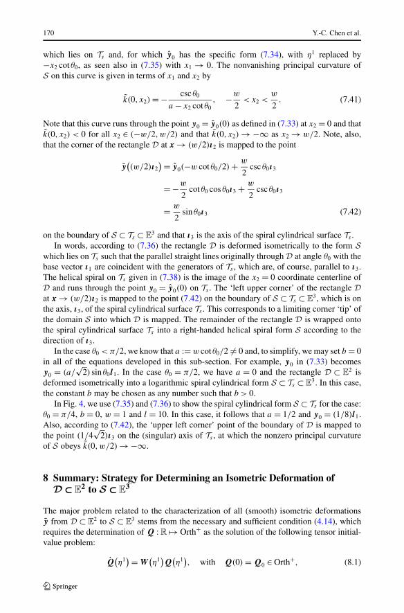
Note that this curve runs through the point y0 = y0(0) as defined in (7.33) at x2 = 0 and thatk(0, x2) < 0 for all x2 ∈ (−w/2,w/2) and that k(0, x2) → −∞ as x2 → w/2. Note, also,that the corner of the rectangle D at x → (w/2)ı2 is mapped to the point
y((w/2)ı2
) = y0(−w cot θ0/2) + w
2csc θ0ı3
= −w
2cot θ0 cos θ0ı3 + w
2csc θ0ı3
= w
2sin θ0ı3 (7.42)
on the boundary of S ⊂ Ts ⊂ E3 and that ı3 is the axis of the spiral cylindrical surface Ts .
In words, according to (7.36) the rectangle D is deformed isometrically to the form Swhich lies on Ts such that the parallel straight lines originally through D at angle θ0 with thebase vector ı1 are coincident with the generators of Ts , which are, of course, parallel to ı3.The helical spiral on Ts given in (7.38) is the image of the x2 = 0 coordinate centerline ofD and runs through the point y0 = y0(0) on Ts . The ‘left upper corner’ of the rectangle Dat x → (w/2)ı2 is mapped to the point (7.42) on the boundary of S ⊂ Ts ⊂ E
3, which is onthe axis, ı3, of the spiral cylindrical surface Ts . This corresponds to a limiting corner ‘tip’ ofthe domain S into which D is mapped. The remainder of the rectangle D is wrapped ontothe spiral cylindrical surface Ts into a right-handed helical spiral form S according to thedirection of ı3.
In the case θ0 < π/2, we know that a := w cot θ0/2 = 0 and, to simplify, we may set b = 0in all of the equations developed in this sub-section. For example, y0 in (7.33) becomesy0 = (a/
√2) sin θ0l1. In the case θ0 = π/2, we have a = 0 and the rectangle D ⊂ E
2 isdeformed isometrically into a logarithmic spiral cylindrical form S ⊂ Ts ⊂ E
3. In this case,the constant b may be chosen as any number such that b > 0.
In Fig. 4, we use (7.35) and (7.36) to show the spiral cylindrical form S ⊂ Ts for the case:θ0 = π/4, b = 0, w = 1 and l = 10. In this case, it follows that a = 1/2 and y0 = (1/8)l1.Also, according to (7.42), the ‘upper left corner’ point of the boundary of D is mapped tothe point (1/4
√2)ı3 on the (singular) axis of Ts , at which the nonzero principal curvature
of S obeys k(0,w/2) → −∞.
8 Summary: Strategy for Determining an Isometric Deformation ofD ⊂ E
2 to S ⊂ E3
The major problem related to the characterization of all (smooth) isometric deformationsy from D ⊂ E
2 to S ⊂ E3 stems from the necessary and sufficient condition (4.14), which
requires the determination of Q : R �→ Orth+ as the solution of the following tensor initial-value problem:
Q(η1
) = W(η1
)Q
(η1
), with Q(0) = Q0 ∈ Orth+, (8.1)

Isometric Deformation of a Planar Material Region into a Curved. . . 171
Fig. 4 Spiral cylindrical helical form of S ⊂ Ts for θ0 = π/4, b = 0, w = 1, and l = 10. The projection ofthe spiral onto the plane spanned by l1 and l2 is also depicted
where W : R �→ Skew is a given field for each η1 ∈ R and a superposed dot denotes dif-ferentiation. Unfortunately, this problem has only been solved in closed form for specialchoices of the skew linear transformation W . If η1 is interpreted as time, (8.1) is a problemwell-known in the field of rigid-body dynamics, in which case W and Q are the angularvelocity tensor and the rotation tensor of the body.
Identifying the importance of problem (8.1) is one of the main conclusions of Sect. 4.Here, we shall summarize in six steps a strategy for the characterization of every isometricdeformation from a region in E
2 to a surfaces in E3 and illustrate how the solution to problem
(8.1) is the key element:
1. Recall from (4.14) that the fundamental proper orthogonal linear transformation Q,which is at the basis for constructing any isometric deformation, must satisfy
ax(QQ�) = λa2,
where λ is scalar-valued and where the unit vector-valued field a2 defines the directionof the straight lines of zero principal curvature on the deformed surface S .
2. Choose λ and a2, and define w by
w(η1
) := λ(η1
)a2
(η1
).
In addition, let W be the skew linear transformation whose axial vector is ax(W ) := w
and note from Step 1 that Q must satisfy
Q(η1
) = W(η1
)Q
(η1
),
in which the field W is now considered to be known. Clearly, if A is the skew lineartransformation whose axial vector is ax(A) := a2, then we may make the following re-placement above: W = λA. Now, the initial condition Q(0) = Q0 ∈ Orth+ must be cho-sen and the now-formulated tensor initial value problem for Q ∈ Orth+ must be solved.Note that this problem is equivalent to (8.1).
3. Determine the unit vector-valued field b2 using (4.9) according to
b2(η1
) = Q�(η1
)a2
(η1
)

172 Y.-C. Chen et al.
and use (4.2b) to determine θ with values in (0,π) according to
b2 = cos θ ı1 + sin θ ı2.
4. Interpret the two parameters η1 and η2 such that all points x ∈ D are located accordingto (4.3), that is
x = x(η1, η2
) = η1ı1 + η2b2
(η1
).
Note, in particular, that this provides a definitive interpretation of the parameter η1 as theη1 (not x1) coordinate of any point x ∈ D.
5. Determine y0 according to (4.11) by integrating
˙y0
(η1
) = Q(η1
)ı1 subject to y0(0) = y0 ∈ E
3.
Here, η1 = 0 is the origin of the midline of the region D in E2 and y0 = y0(0) is specified
as the limit point in E3 where x → x(0,0) = 0 is to be transformed under the isometric
deformation y from D to S .8
6. Determine the component y of the parametric representation of the isometric deformationy defined implicitly through (4.3) and (4.6), in accord with
y(η1, η2
) = y0
(η1
) + η2Q(η1
)b2
(η1
)
= y0
(η1
) + η2a2(η1
).
Finally, after determining the form of the isometric deformation y by replacing (η1, η2)
in Step 6 with (x1, x2) using Step 4, observe that the curvature tensor for S is given by(6.12).
9 Isometric Deformation of a Rectangular Material Strip D ⊂ E2 to
Portion S of a Conical Surface K ⊂ E3
Suppose that D is the rectangle of length l and width w consisting of all points x = xiıi
with rectilinear coordinates x1 and x2 restricted as in (7.15) and shown in Fig. 2. Let K ⊂ E3
denote a right conical surface with circular base of radius R in the plane spanned by ı1 andı2 and tip located at H ı3. The tip angle of K is then equal to 2ϕ, where ϕ ∈ (0,π/2) satisfies
tanϕ = R
H. (9.1)
The cone K is allowed to extend without limit in the −ı3 direction but, for convenience andwith a slight abuse of terminology, we continue to refer to its base as the plane spanned by ı1
and ı2. The objective of this section is to identify a general isometric deformation of D ⊂ E2
to S ⊂ K ⊂ E3 using the strategy outlined above in Sect. 8.
8Convenient appropriate choices for y0 are shown the examples in Sects. 7.1 and 7.2.

Isometric Deformation of a Planar Material Region into a Curved. . . 173
9.1 General Case
To begin, following Steps 1 and 2 in Sect. 8, we suppose that there is a smooth family ofdistinct straight lines that foliate and intersect with D, as generally illustrated in Fig. 1. Theunit vector field b2 that characterizes these straight lines was introduced in (4.2b) as
b2
(η1
) = cos θ(η1
)ı1 + sin θ
(η1
)ı2, (9.2)
where η1ı1 the point where each straight line cuts through the x1-coordinate line and θ(η1) ∈(0,π) is the angle of b2(η
1) measured from ı1. These lines are the pre-images in D of thestraight lines of zero curvature in S ⊂ K to which D is isometrically deformed. Accordingto (4.7) and (4.9), these lines are related to b2 by
a2
(η1
) = Q(η1
)b2
(η1
), (9.3)
and we are to determine Q ∈ Orth+ such that
Q(η1
) = λ(η1
)A
(η1
)Q
(η1
), with Q(0) = Q0, (9.4)
where Q0 ∈ Orth+ is prescribed, A ∈ Skew is given with a2 = ax(A) and the scalar-valuedfield λ is assumed known, but is to be determined later.
To analyze (9.4), we first need to characterize the skew tensor A whose axial vector is a2.Toward this end, note that since the straight line generators of the conical surface K are thelines of zero curvature on S ⊂ K and that a2 is parallel to these lines, we may write
a2
(η1
) = Q1
(η1
)a, (9.5)
where
a := −Rı1 + H ı3√R2 + H 2
= − sinϕı1 + cosϕı3 (9.6)
is the direction of the specific generator from the point Rı1 on the base of K to the pointH ı3 at its tip, and
Q1
(η1
) := eω(η1)A1 , A1 := −ı1 ⊗ ı2 + ı2 ⊗ ı1, (9.7)
represents a right-handed rotation of angle ω about the ı3 = ax(A1) axis. We set ω(0) = 0,so that Q1(0) = 1 and a2(0) = a. An alternative representation for Q1 is
Q1
(η1
) = cosω(η1
)(ı1 ⊗ ı1 + ı2 ⊗ ı2) − sinω
(η1
)(ı1 ⊗ ı2 − ı2 ⊗ ı1) + ı3 ⊗ ı3 (9.8)
and we find, using (9.5), (9.6), and (9.8), that
a2
(η1
) = − sinϕ(cosω
(η1
)ı1 + sinω
(η1
)ı2
) + cosϕı3. (9.9)
Since a2 is the axial vector of A, we see that
A(η1
) = cosϕ(−ı1 ⊗ ı2 + ı2 ⊗ ı1)
+ sinω(η1
)sinϕ(−ı1 ⊗ ı3 + ı3 ⊗ ı1)
+ cosω(η1
)sinϕ(ı2 ⊗ ı3 − ı3 ⊗ ı2). (9.10)
174 Y.-C. Chen et al.
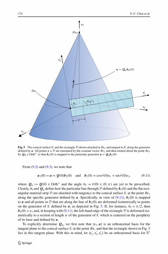
Fig. 5 The conical surface K and the rectangle D shown attached at Rı1 and tangent to K along the generatordefined by a. All points x ∈ D are translated by the constant vector Rı1 and then rotated about the point Rı1by Q0 ∈ Orth+ so that b2(0) is mapped to the particular generator a = Q0b2(0)
From (9.2) and (9.3), we note that
a2(0) = a = Q(0)b2(0) and b2(0) = cos θ(0)ı1 + sin θ(0)ı2, (9.11)
where Q0 := Q(0) ∈ Orth+ and the angle θ0 := θ(0) ∈ (0,π) are yet to be prescribed.Clearly, θ0 and Q0 define how the particular line through D defined by b2(0) and the flat rect-angular material strip D are attached with tangency to the conical surface K at the point Rı1
along the specific generator defined by a. Specifically, in view of (9.11), b2(0) is mappedto a and all points in D that are along the line of b2(0) are deformed isometrically to pointson the generator of K defined by a, as depicted in Fig. 5. If, for instance, θ0 = π/2, thenb2(0) = ı2 and, in keeping with (9.11), the left-hand edge of the rectangle D is deformed iso-metrically to a section of length w of the generator of K which is centered on the peripheryof its base and defined by a.
To explicitly determine Q0, we first note that {ı2,a} is an orthonormal basis for thetangent plane to the conical surface K at the point Rı1 and that the rectangle shown in Fig. 5lies in this tangent plane. With this in mind, let {ı ′
1, ı′2, ı
′3} be an orthonormal basis for E3
Isometric Deformation of a Planar Material Region into a Curved. . . 175
such that the basis {ı ′1, ı
′2} with
ı ′1 := sin θ0ı2 + cos θ0a and ı ′
2 := − cos θ0ı2 + sin θ0a (9.12)
lies in the tangent plane to K at Rı1, as indicated in Fig. 5. Of course,
ı ′3 := ı ′
1 × ı ′2 = ı2 × a. (9.13)
Also, observe that ı ′i = Q0ıi for i = 1,2, that ı ′
3 = Q0ı3, that Q0 = ı ′i ⊗ ıi + ı ′
3 ⊗ ı3 ∈ Orth+,and that (9.11) holds. Specifically, we find that
Q0 = − cos θ0 sinϕı1 ⊗ ı1 − sin θ0 sinϕı1 ⊗ ı2 + cosϕı1 ⊗ ı3
+ sin θ0ı2 ⊗ ı1 − cos θ0ı2 ⊗ ı2 + cos θ0 cosϕı3 ⊗ ı1
+ sin θ0 cosϕı3 ⊗ ı2 + sinϕı3 ⊗ ı3. (9.14)
On applying Q0 to the rectangular material strip D and translating the origin of the stripat x = 0 to the point Rı1, the strip remains flat, the left-hand end becomes tangent to theconical surface K at the point Rı1, and the midline of the strip becomes coincident with ı ′
1.The next step is to find Q such that the strip is wrapped isometrically onto the conicalsurface K, in agreement with the ‘initial condition’ Q(0) = Q0.
For convenience, we suppress dependence on the independent variable η1 whenever pos-sible in the following development and rewrite (9.4), using (9.7)2 and (9.10), as
QQ� = λ(cosϕA1 − sinϕ sinω(ı1 ⊗ ı3 − ı3 ⊗ ı1)− sinϕ cosω(ı3 ⊗ ı2 − ı2 ⊗ ı3)
). (9.15)
After some consideration, the structure of the right-hand side of (9.15) and the conditionQ(0) = Q0 suggest that we look for Q in the form
Q = Q1Q0Q2, (9.16)
where Q1 is as defined in (9.7) (see also (9.8)) and Q2 is defined as
Q2
(η1
) := eξ(η1)A1 , A1 := −ı1 ⊗ ı2 + ı2 ⊗ ı1, (9.17)
with ξ to be determined such that ξ(0) = 0 and, thus, that Q2(0) = 1 . Following this propo-sition, we then see that
QQ� = Q1Q�1 + Q1Q0Q2Q
�2 Q�
0 Q�1 = ωA1 + ξQ1Q0A1Q
�0 Q�
1 , (9.18)
and a short calculation using (9.6) and (9.14) yields
Q0A1Q�0 = a ⊗ ı2 − ı2 ⊗ a. (9.19)
With the aid of (9.5), (9.8), and (9.9), it then follows that
Q1Q0A1Q�0 Q�
1 = Q1(a ⊗ ı2 − ı2 ⊗ a)Q�1 = a2 ⊗ Q1ı2 − Q1ı2 ⊗ a2
= sinϕ(−ı1 ⊗ ı2 + ı2 ⊗ ı1) + sinω cosϕ(ı1 ⊗ ı3 − ı3 ⊗ ı1)
+ cosω cosϕ(ı3 ⊗ ı2 − ı2 ⊗ ı3)
= sinϕA1 + sinω cosϕ(ı1 ⊗ ı3 − ı3 ⊗ ı1)
+ cosω cosϕ(ı3 ⊗ ı2 − ı2 ⊗ ı3). (9.20)

176 Y.-C. Chen et al.
Thus, with (9.15), (9.18), and (9.20) we find that
ω + ξ sinϕ = λ cosϕ and ξ cosϕ = −λ sinϕ, (9.21)
and, thus, that λ takes the form
λ(η1
) = ω(η1
)cosϕ, (9.22)
and, moreover, that ξ = −ω sinϕ which, when integrated subject to the requirement ω(0) =ξ(0) = 0, gives
ξ(η1
) = −ω(η1
)sinϕ. (9.23)
Finally, with the conclusions of (9.22), (9.23), and (9.14) we have found that Q determinedaccording to (9.16) with Q1 and Q2 given by
Q1 = eωA1 , Q2 = e−ω sinϕA1 , A1 = −ı1 ⊗ ı2 + ı2 ⊗ ı1, (9.24)
solves the tensor initial value problem (9.4), namely
QQ� = λA, with Q(0) = Q0, (9.25)
with λ given by (9.22).We now turn to Step 3 of Sect. 8 to determine the scalar field θ and return to (9.3) and
(9.5) to see that
Q1a = Qb2 = Q1Q0Q2b2, (9.26)
from which it follows that we must have a = Q0Q2b2. Then, since (9.11) gives a =Q0b2(0), we readily arrive at b2(0) = Q2b2, or the equivalent relation
cos θ0ı1 + sin θ0ı2 = Q2(cos θ ı1 + sin θ ı2). (9.27)
Now, observing from (9.24) that Q2 corresponds to a rotation about −ı3 of angle ω sinϕ, iteasily follows that
cos θ0ı1 + sin θ0ı2 = cos(θ − ω sinϕ)ı1 + sin(θ − ω sinϕ)ı2, (9.28)
with the consequence that
θ(η1
) − θ0 = ω(η1
)sinϕ. (9.29)
This relationship (9.29) between θ and ω has a natural and clear interpretation. To expressthis, recall that the straight lines which intersect D ⊂ E
2 at the angle θ0 = θ(0) at the ori-gin point η1ı1 = 0 and at the angle θ(η1) at the point η1ı1 are supposed to correspond totwo straight lines of zero curvature on S ⊂ K ⊂ E
3. These, of course, are two straight linegenerators of the conical surface K on which S lies. Recall, also, that R is the radius of thebase of K and H is its height. Thus, the length of the generator from the base of K to its tipis L := √
R2 + H 2 and the tip angle 2ϕ satisfies sinϕ = R/L. Accordingly, (9.29) may bewritten as
L(θ(η1
) − θ0
) = Rω(η1
), (9.30)
which implies that, for each choice of η1, the arc length of the sector of a circle of radiusL in E
2 that spans the angle θ(η1) − θ0 is equal to the arc length of the sector of the circle
Isometric Deformation of a Planar Material Region into a Curved. . . 177
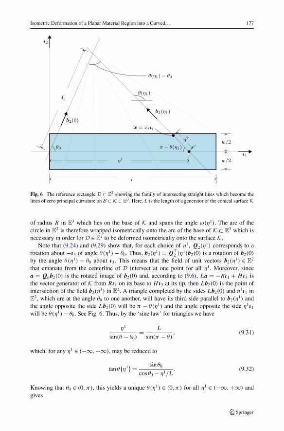
Fig. 6 The reference rectangle D ⊂ E2 showing the family of intersecting straight lines which become the
lines of zero principal curvature on S ⊂K ⊂ E3. Here, L is the length of a generator of the conical surface K
of radius R in E3 which lies on the base of K and spans the angle ω(η1). The arc of the
circle in E2 is therefore wrapped isometrically onto the arc of the base of K ⊂ E
3 which isnecessary in order for D ∈ E
2 to be deformed isometrically onto the surface K.Note that (9.24) and (9.29) show that, for each choice of η1, Q2(η
1) corresponds to arotation about −ı3 of angle θ(η1) − θ0. Thus, b2(η
1) = Q�2 (η1)b2(0) is a rotation of b2(0)
by the angle θ(η1) − θ0 about ı3. This means that the field of unit vectors b2(η1) ∈ E
2
that emanate from the centerline of D intersect at one point for all η1. Moreover, sincea = Q0b2(0) is the rotated image of b2(0) and, according to (9.6), La = −Rı1 + H ı3 isthe vector generator of K from Rı1 on its base to H ı3 at its tip, then Lb2(0) is the point ofintersection of the field b2(η
1) in E2. A triangle completed by the sides Lb2(0) and η1ı1 in
E2, which are at the angle θ0 to one another, will have its third side parallel to b2(η
1) andthe angle opposite the side Lb2(0) will be π − θ(η1) and the angle opposite the side η1ı1
will be θ(η1) − θ0. See Fig. 6. Thus, by the ‘sine law’ for triangles we have
η1
sin(θ − θ0)= L
sin(π − θ), (9.31)
which, for any η1 ∈ (−∞,+∞), may be reduced to
tan θ(η1
) = sin θ0
cos θ0 − η1/L. (9.32)
Knowing that θ0 ∈ (0,π), this yields a unique θ(η1) ∈ (0,π) for all η1 ∈ (−∞,+∞) andgives

178 Y.-C. Chen et al.
θ(η1
) = sin2 θ(η1)
L sin θ0> 0. (9.33)
Following Step 4 in Sect. 8, we recall that each point x of the rectangular material stripD is to be located by the coordinates (η1, η2) by
x = x(η1, η2
) = η1ı1 + η2b2
(η1
), (9.34)
with b2 given by
b2(η1
) = cos θ(η1
)ı1 + sin θ
(η1
)ı2, (9.35)
as illustrated in Fig. 6. It is an exercise in trigonometry, using (9.32), to show that the(η1, η2) coordinates of the bottom and top left corners on the boundary of D are (d+
l , k+l )
and (d−l , k−
l ), respectively, with
d±l := ±w
2
cos θ0
sin θ0 ± w/2L, k±
l := ∓√
(d±
l
)2 +(
w
2
)2
, (9.36)
while, by (9.35), b2 has corresponding values
b2
(d±
l
) := |d±l |ı1 + wı2/2
k±l
. (9.37)
Clearly, the values of η1 determined above make sense only if the width w of the rectangleis not too large compared to the length L of the generator of the conical surface K—that is,only if w < 2L sin θ0. Otherwise, the apex of K is involved with the isometric deformationof D to S and the nonvanishing principal curvature of S is unbounded.9
Similarly, the (η1, η2) coordinates of the bottom and top right corners on the boundaryof D are (l + d+
r , k+r ) and (l + d−
r , k−r ), respectively, with
d±r := ∓w
2
l/L − cos θ0
sin θ0 ± w/2L, k±
r := ∓√
(d±
r
)2 +(
w
2
)2
, (9.38)
while, by (9.35), b2 has corresponding values
b2
(l + d±
r
) := −|d±r |ı1 + wı2/2
k±r
. (9.39)
Referring to Step 5 in Sect. 8, we next determine the curve on the conical surface K thatdefines the midline of the rectangular material strip D under the isometric deformation of Dto S ⊂ K. This is given by the field y0 determined by integrating
˙y0
(η1
) = Q(η1
)ı1, with y0(0) = Rı1, (9.40)
where Q = Q1Q0Q2 is given through (9.14) and (9.24)–(9.32).
9We calculate the nonzero principal curvature of S in (9.58) and show how the inequality w < 2L sin θ0arises from the condition that the curvature of S is bounded. Due to this inequality, the nonvanishing principalcurvature is, in fact, everywhere negative on S .
Isometric Deformation of a Planar Material Region into a Curved. . . 179
Using Q0 from (9.14) and the alternative form
Q2 = cos(ω sinϕ)(ı1 ⊗ ı1 + ı2 ⊗ ı2) + sin(ω sinϕ)(ı1 ⊗ ı2 − ı2 ⊗ ı1) + ı3 ⊗ ı3 (9.41)
of Q2 from (9.24), we find, upon using (9.29), that
Q0Q2 = − sinϕ cos θ ı1 ⊗ ı1 − sinϕ sin θ ı1 ⊗ ı2 + cosϕı1 ⊗ ı3 + sin θ ı2 ⊗ ı1
− cos θ ı2 ⊗ ı2 + cosϕ cos θ ı3 ⊗ ı1 + cosϕ sin θ ı3 ⊗ ı2
+ sinϕı3 ⊗ ı3. (9.42)
Thus,
Q0Q2ı1 = − sinϕ cos θ ı1 + sin θ ı2 + cosϕ cos θ ı3, (9.43)
and, with the alternative form (9.8) of Q1, we have
Q(η1
)ı1 = Q1
(η1
)Q0Q2
(η1
)ı1
= −(cosω
(η1
)sinϕ cos θ
(η1
) + sinω(η1
)sin θ
(η1
))ı1
− (sinω
(η1
)sinϕ cos θ
(η1
) − cosω(η1
)sin θ
(η1
))ı2
+ cosϕ cos θ(η1
)ı3. (9.44)
Thus, integrating (9.40) yields
y0
(η1
) =(
R −∫ η1
0
(cosω(x) sinϕ cos θ(x) + sinω(x) sin θ(x)
)dx
)ı1
−(∫ η1
0
(sinω(x) sinϕ cos θ(x) − cosω(x) sin θ(x)
)dx
)ı2
+(∫ η1
0cosϕ cos θ(x)dx
)ı3, (9.45)
where, according to (9.29),
ω(x) = θ(x) − θ0
sinϕ, (9.46)
and, from (9.32),
tan θ(x) = sin θ0
cos θ0 − x/L, −∞ < x < +∞. (9.47)
In view of (9.33), we may change the variable of integration from x to θ , giving
y0
(η1
) =(
R − L sin θ0
∫ θ(η1)
θ0
(cos
(θ − θ0
sinϕ
)sinϕ cot θ + sin
(θ − θ0
sinϕ
))csc θ dθ
)ı1
−(∫ θ(η1)
θ0
(sin
(θ − θ0
sinϕ
)sinϕ cot θ − cos
(θ − θ0
sinϕ
))csc θ dθ
)ı2
+(∫ θ(η1)
θ0
cosϕ cot θ csc θ dθ
)ı3. (9.48)

180 Y.-C. Chen et al.
However, it does not appear possible to integrate (9.48) in closed form for general choicesof θ0 ∈ (0,π) and ϕ ∈ (0,π/2).
Turning to Step 6 in Sect. 8, we next determine the component y of the isometric defor-mation y of D ⊂ E
2 to S ⊂ K ⊂ E3 defined implicitly through (4.3) and (4.6), i.e.,
y(η1, η2
) = y0
(η1
) + η2Q(η1
)b2
(η1
), (9.49)
where y0 is given in (9.48) and, by (9.3), (9.9), and (9.29),
Q(η1
)b2
(η1
) = a2
(η1
) = − sinϕ(cosω
(η1
)ı1 + sinω
(η1
)ı2
) + cosϕı3, (9.50)
with
ω(η1
) = θ(η1) − θ0
sinϕ. (9.51)
The angle θ is determined from (9.32) and the monotonically increasing condition (9.33),from which we may write
sin θ(η1
) = sin θ0√sin2 θ0 + (cos θ0 − η1/L)2
,
cos θ(η1
) = cos θ0 − η1/L√
sin2 θ0 + (cos θ0 − η1/L)2.
⎫⎪⎪⎪⎪⎬
⎪⎪⎪⎪⎭
(9.52)
Finally, to completely characterize the isometric deformation y, we need only to evaluate
y = y(η1, η2
) = y0
(η1
) − η2(sinϕ
(cosω
(η1
)ı1 + sinω
(η1
)ı2
) − cosϕı3
), (9.53)
for all (η1, η2) that correspond to the points x ∈ D through (4.1b), which can be expressedas
η1 = x1 − x2 cot θ(η1
)and η2 = x2 csc θ
(η1
). (9.54)
With (9.32), the first of (9.54) gives
η1 = x1 − x2 cot θ0
1 − x2 csc θ0/L, (9.55)
for all (x1, x2) ∈ (0, l)× (−w/2,w/2). Then, observing that (9.54) implies that (η1 −x1)2 +
(x2)2 = (η2)2 and knowing that 0 < θ < π , the second of (9.54) gives
η2 = sgn(x2)
√(η1 − x1
)2 + x22 , (9.56)
for all (x1, x2) ∈ (0, l) × (−w/2,w/2), which, with (9.55), yields
η2 = x2
√
1 +(
cos θ0 − x1/L
sin θ0 − x2/L
)2
, (9.57)
for all (x1, x2) ∈ (0, l) × (−w/2,w/2). Clearly, (9.55) and (9.57) make sense only if w <
2L sin θ0, confirming what we reported earlier in the discussion following (9.34) concerningthe location of the bottom and top corners on the boundary of D in terms of the coordinates(η1, η2).10
10See also the interpretation of (9.58), below.

Isometric Deformation of a Planar Material Region into a Curved. . . 181
The nonvanishing principal curvature k of the deformed surface S is obtained from(6.13), (9.22), (9.29), and (9.33) as
k(η1, η2
) = − cotϕ sin θ(η1)
L sin θ0(1 − η2 sin θ(η1)/L sin θ0). (9.58)
Thus, because (9.33) readily yields
η2θ(η1
) − sin θ(η1
) = − sin θ(η1
)(
1 − η2 sin θ(η1)
L sin θ0
), (9.59)
it follows from (4.4) that the denominator in (9.58) is restricted away from zero. Since x2 isin the interval (−w/2,w/2), it follows from (9.54)2 that this restriction is equivalent to w <
2L sin θ0. Consequently, k is strictly negative for all points x ∈ D. With the additional use of(9.52)1, (9.55), and (9.58) we may represent k in terms of (x1, x2) ∈ (0, l) × (−w/2,w/2)
in the form
k(x1, x2) := − cotϕ
L√
(cos θ0 − x1/L)2 + (sin θ0 − x2/L)2, (9.60)
from which it is clear that the restriction w < 2L sin θ0 keeps k bounded and negative for allx ∈ D.
9.2 Particular Example
For illustrative purposes, we choose
θ0 = π
4and ϕ = π
6, (9.61)
in which case, the dimensions L and R of the conical surface K satisfy
L = 2R (9.62)
and from (9.29) we have
ω = 2θ − π
2. (9.63)
With (9.63) and the aid of common trigonometric identities we find that (9.48) yields
y0
(η1
) = √2R
(cos θ
(η1
)ı1 +
(sin θ
(η1
) − csc θ(η1)
2
)ı2 +
√3
2
(1 − csc θ(η1)√
2
)ı3
).
(9.64)In addition, (9.53) reduces to
y = y(η1, η2
) = y0
(η1
) − η2
2
(sin 2θ
(η1
)ı1 + cos 2θ
(η1
)ı2 − √
3ı3). (9.65)
In these equations we need to substitute for the field θ from (9.32), which in view of (9.61)and (9.62) reduces to
tan θ(η1
) = 1
1 − η1/√
2R. (9.66)
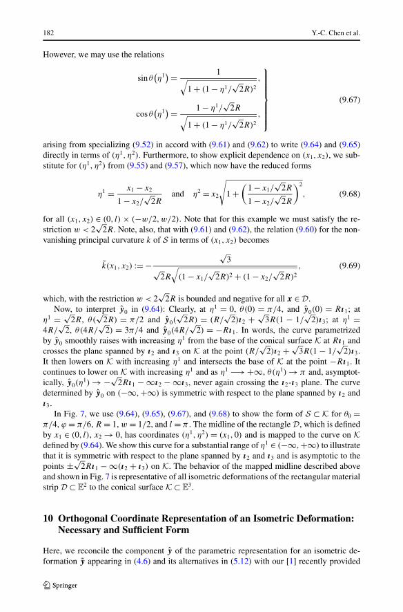
182 Y.-C. Chen et al.
However, we may use the relations
sin θ(η1
) = 1√
1 + (1 − η1/√
2R)2
,
cos θ(η1
) = 1 − η1/√
2R√
1 + (1 − η1/√
2R)2
,
⎫⎪⎪⎪⎪⎪⎪⎬
⎪⎪⎪⎪⎪⎪⎭
(9.67)
arising from specializing (9.52) in accord with (9.61) and (9.62) to write (9.64) and (9.65)directly in terms of (η1, η2). Furthermore, to show explicit dependence on (x1, x2), we sub-stitute for (η1, η2) from (9.55) and (9.57), which now have the reduced forms
η1 = x1 − x2
1 − x2/√
2Rand η2 = x2
√
1 +(
1 − x1/√
2R
1 − x2/√
2R
)2
, (9.68)
for all (x1, x2) ∈ (0, l) × (−w/2,w/2). Note that for this example we must satisfy the re-striction w < 2
√2R. Note, also, that with (9.61) and (9.62), the relation (9.60) for the non-
vanishing principal curvature k of S in terms of (x1, x2) becomes
k(x1, x2) := −√
3√
2R
√(1 − x1/
√2R)2 + (1 − x2/
√2R)2
, (9.69)
which, with the restriction w < 2√
2R is bounded and negative for all x ∈ D.Now, to interpret y0 in (9.64): Clearly, at η1 = 0, θ(0) = π/4, and y0(0) = Rı1; at
η1 = √2R, θ(
√2R) = π/2 and y0(
√2R) = (R/
√2)ı2 + √
3R(1 − 1/√
2)ı3; at η1 =4R/
√2, θ(4R/
√2) = 3π/4 and y0(4R/
√2) = −Rı1. In words, the curve parametrized
by y0 smoothly raises with increasing η1 from the base of the conical surface K at Rı1 andcrosses the plane spanned by ı2 and ı3 on K at the point (R/
√2)ı2 + √
3R(1 − 1/√
2)ı3.It then lowers on K with increasing η1 and intersects the base of K at the point −Rı1. Itcontinues to lower on K with increasing η1 and as η1 −→ +∞, θ(η1) → π and, asymptot-ically, y0(η
1) → −√2Rı1 − ∞ı2 − ∞ı3, never again crossing the ı2-ı3 plane. The curve
determined by y0 on (−∞,+∞) is symmetric with respect to the plane spanned by ı2 andı3.
In Fig. 7, we use (9.64), (9.65), (9.67), and (9.68) to show the form of S ⊂ K for θ0 =π/4, ϕ = π/6, R = 1, w = 1/2, and l = π . The midline of the rectangle D, which is definedby x1 ∈ (0, l), x2 → 0, has coordinates (η1, η2) = (x1,0) and is mapped to the curve on Kdefined by (9.64). We show this curve for a substantial range of η1 ∈ (−∞,+∞) to illustratethat it is symmetric with respect to the plane spanned by ı2 and ı3 and is asymptotic to thepoints ±√
2Rı1 − ∞(ı2 + ı3) on K. The behavior of the mapped midline described aboveand shown in Fig. 7 is representative of all isometric deformations of the rectangular materialstrip D ⊂ E
2 to the conical surface K ⊂ E3.
10 Orthogonal Coordinate Representation of an Isometric Deformation:Necessary and Sufficient Form
Here, we reconcile the component y of the parametric representation for an isometric de-formation y appearing in (4.6) and its alternatives in (5.12) with our [1] recently provided

Isometric Deformation of a Planar Material Region into a Curved. . . 183
Fig. 7 Conical form of S ⊂ K for θ0 = π/4, ϕ = π/6, R = 1, w = 1/2, and l = π
representation. To achieve that, we identify the curvilinear coordinates (ζ 1, ζ 2) with the co-ordinate curves (α,β) introduced in Sect. 3, where the transformation (x1, x2) ←→ (ζ 1, ζ 2)
is defined by
x = xiıi = xi
(ζ 1, ζ 2
)ıi
= x(ζ 1, ζ 2
) := x0(ζ 1
) + ζ 2(cos θ
(ζ 1
)ı1 + sin θ
(ζ 1
)ı2
), (10.1a)
with
x0(ζ 1
) :=∫ ζ 1
0
(sin θ (u)ı1 − cos θ (u)ı2
)du. (10.1b)

184 Y.-C. Chen et al.
Fig. 8 Coordinates for x ∈ D in terms of (ζ 1, ζ 2). The curve C0 is indicated in red and the arclength betweenthe two red points on C0 is given by ζ 1
Here, x0 parametrizes a curve C0 that passes through the origin x = 0 and has unit tangentvector x ′
0 given by
x ′0
(ζ 1
) = sin θ(ζ 1
)ı1 − cos θ
(ζ 1
)ı2, (10.2)
where a prime is used to denote differentiation with respect to ζ 1. The ζ 1-coordinate line iscoincident with the curve C0 at ζ 2 = 0 and the ζ 2-coordinate lines run along straight lines inD that correspond to pre-images of the straight lines of zero principal curvature in S . Theζ 2-coordinate line passing through (ζ 1,0) forms an angle θ (ζ 1) ∈ (0,π) with the x1-axis asshown in Fig. 8.
The curve C0 is clearly orthogonal to the ζ 2-coordinate lines and the ζ 1-coordinate linescorresponding to ζ 2 = constant are not straight unless θ is constant. The base vectors of V2
through each x ∈ D ⊂ E2 for the curvilinear system are given by
gi = ∂x
∂ζ i= ∂xm
∂ζ i
∂x
∂xm
= ∂xm
∂ζ iım, i = 1,2, (10.3a)
so that
g1 = ∂x
∂ζ 1= (
1 − ζ 2θ ′)(sin θ ı1 − cos θ ı2),
g2 = ∂x
∂ζ 2= cos θı1 + sin θ ı2,
⎫⎪⎪⎬
⎪⎪⎭(10.3b)
Isometric Deformation of a Planar Material Region into a Curved. . . 185
where the dependencies of g1, g2, and θ on ζ 1 are suppressed for brevity. Note, from(10.3b), that |g1| = |1 − ζ 2θ ′|, |g2| = 1, and g1 · g2 = 0, whereby {g1,g2} is an orthog-onal basis. Moreover, (10.1a) takes the explicit form
x = x(ζ 1, ζ 2
) = x0
(ζ 1
) + ζ 2g2
(ζ 1
). (10.4)
To ensure that {g1,g2} is an acceptable basis for representing the points of D ⊂ E2, we
restrict θ and ζ 2 so that
det(gi · gj ) := |g1|2|g2|2 − (g1 · g2)2 = |g1|2 = (
1 − ζ 2θ ′)2 = 0 (10.5)
on D.11
Now, setting α = ζ 1, β = ζ 2, b(α) = g2(ζ1), and Q(α) = Q(ζ 1) in (3.43), defining a
mapping y of (ζ 1, ζ 2) to S such that
y(ζ 1, ζ 2
) = y(x(ζ 1, ζ 2
)), (10.6)
and writing y0 = y(·,0) for the parametrization of the image in S of the ζ 2 = 0 coordinateline C0 in D, we arrive at the representation
y = y(ζ 1, ζ 2
) = y0
(ζ 1
) + ζ 2Q(ζ 1
)g2
(ζ 1
). (10.7)
From here we easily see that
ai := ∂y
∂ζ i= ∂xm
∂ζ iy,m = ∂xm
∂ζ iem. (10.8)
Thus, because (10.3a) implies that
∂xm
∂ζ i= ım · gi (10.9)
and because em = Qım, we obtain
ai = em(ım · gi ) = (Qım ⊗ ım)gi = Qgi , i = 1,2, (10.10)
which yields a1 · a2 = 0 and |ai | = |gi |. In particular, we see that |a1| = |1 − ζ 2θ ′|, |a2| = 1and that a2 defines the field of straight lines of zero curvature in S that associate with thestraight lines given by g2 in D. Note that (10.7) implies that
a1 = ∂y
∂ζ 1= y ′
0 + ζ 2(Q
′g2 + Qg′
2
), (10.11)
where
y ′0
(ζ 1
) = ∂y(ζ 1,0)
∂ζ 1= a1
(ζ 1,0
) = Q(ζ 1
)g1
(ζ 1,0
) = Q(sin θı1 − cos θ ı2), (10.12)
and that from (10.3b) we have
ζ 2g′2 = −ζ 2(− sin θ ı1 − cos θ ı2)θ
′ = g1 − sin θ ı1 + cos θ ı2. (10.13)
11We shall see in (10.69) that the restriction (10.5) is related to the possible unboundedness of the curvatureof S .

186 Y.-C. Chen et al.
Thus, recalling from (10.10) that a1 = Qg1, we see from (10.11) that Q must satisfy
Q′g2 = 0, (10.14)
which is a necessary condition on how the proper orthogonal transformation field Q must bechosen to ensure that, in conjunction with (10.4), (10.7) provides a parametric representationof an isometric deformation y. It readily follows from (10.10) that (10.14) is equivalent to
Q′Q
�a2 = 0, which means that the “angular velocity” corresponding to Q, namely the
axial vector ax(Q′Q
�) of the skew linear transformation Q
′Q
�, must be parallel to a2,
the lines L of zero principal curvature in S . There thus exist a scalar field λ and a skewlinear transformation A with axial unit vector a2, both generally dependent only on ζ 1 butindependent of ζ 2, such that
ax(Q
′Q
�) = λa2 and Q′Q
� = λA. (10.15)
Of course, |λ| = |ax(Q′Q
�)|.
The condition (10.14) is not only necessary for the parametric representation of the de-formation y of D ⊂ E
2 to S ⊂ E3 as defined implicitly by (10.4) and (10.7) to be an isometricdeformation, but it is also sufficient. To see this, first observe from (10.6), (10.7), and (10.11)that
∇y := ∂y
∂ζ i⊗ gi = (
y ′0 + ζ 2
(Q
′g2 + ζ 2Qg′
2
)) ⊗ g1 + Qg2 ⊗ g2, (10.16)
where {g1,g2}, with
g1 := sin θ ı1 − cos θ ı2
1 − ζ 2θ ′ and g2 := cos θı1 + sin θ ı2 (10.17)
is the basis of V2 dual to {g1,g2}.Next, we observe that (10.12)–(10.14) allow us to write
∇y = Qg1 ⊗ g1 + Qg2 ⊗ g2 = Q(g1 ⊗ g1 + g2 ⊗ g2
), (10.18)
which is equivalent to
∇y = Q(ı1 ⊗ ı1 + ı2 ⊗ ı2). (10.19)
Thus, because Q ∈ Orth+,
(∇y)�∇y = (ı1 ⊗ ı1 + ı2 ⊗ ı2)Q�Q(ı1 ⊗ ı1 + ı2 ⊗ ı2) = ı1 ⊗ ı1 + ı2 ⊗ ı2, (10.20)
and this ensures that the length between any two points in D is preserved under the defor-mation y provided (10.14) holds.
10.1 The Isometric Deformation y in Terms of the Curve C ∈ S and ItsCoordinate Pre-image Curve C0 ∈ D
Note, from (10.12), that the unit tangent vector to the space curve C parametrized by y0 isgiven by
t := y ′0 = Q(sin θ ı1 − cos θ ı2), (10.21)

Isometric Deformation of a Planar Material Region into a Curved. . . 187
and recall that the Frenet triad {t, p, b} of tangent, normal and bi-normal unit vectors, re-spectively, for this curve are related according to
p := t′
|t ′| and b := t × p, (10.22)
for t′ = 0. Moreover, this triad satisfies the Frenet–Serret relations
t′ = κp, p′ = −κ t + τ b, b
′ = −τ p, (10.23)
where κ := −p′ · t and τ := p′ · b denote, respectively, the curvature and torsion of the curveC parametrized by y0.
Now, using Q′ = λAQ from (10.15)2 and employing (10.3b)2, (10.10), and the relation
n = Qı3 =: n, (10.24)
which follows from (3.39) and our earlier replacement of Q by Q in (3.43) to arrive at(10.7), we see that
t′ = Q
′(sin θ ı1 − cos θ ı2) + θ ′Q(cos θ ı1 + sin θ ı2)
= λAQ(sin θ ı1 − cos θı2) + θ ′Qg2
= λa2 × Q(sin θ ı1 − cos θ ı2) + θ ′Qg2
= λQ(g2 × (sin θ ı1 − cos θ ı2)
) + θ ′Qg2
= Q(−λı3 + θ ′g2
)
= −λn + θ ′a2. (10.25)
Thus, it follows that |t ′| =√
λ2 + (θ ′)2 and by introducing a field ϕ, with values in [0,2π),defined such that
sin ϕ = λ√
λ2 + (θ ′)2and cos ϕ = θ ′
√λ2 + (θ ′)2
, (10.26)
we may write
p = − sin ϕn + cos ϕa2. (10.27)
Also, because
t × a2 = Q(sin θ ı1 − cos θ ı2) × Qg2
= Q((sin θ ı1 − cos θ ı2) × g2
) = Qı3 = n (10.28)
and
t × n = Q(sin θ ı1 − cos θ ı2) × Qı3
= Q(− sin θı2 − cos θ ı1) = −Qg2 = −a2, (10.29)
188 Y.-C. Chen et al.
we see that {t, a2, n} provides a positively-oriented orthonormal basis for V3 and, moreover,that the Frenet binormal of the curve parametrized by y0 is given by
b = sin ϕa2 + cos ϕn. (10.30)
As an immediate consequence of (10.27) and (10.30), we find that
a2 = cos ϕp + sin ϕb. (10.31)
Moreover, differentiating (10.27) and using (10.30), we obtain
p′ = (− cos ϕn − sin ϕa2)ϕ′ − sin ϕn′ + cos ϕa′
2
= −ϕ′b − sin ϕn′ + cos ϕa′2. (10.32)
Thus, as a consequence of the identities
n′ = Q′ı3 = λAQı3 = λa2 × n = λt (10.33a)
and
a′2 = Q
′g2 + Qg′
2 = Qg′2 = Q(− sin θ ı1 + cos θ ı2)θ
′ = −θ ′ t, (10.33b)
it follows, using (10.26), that
p′ = −ϕ′b − (λ sin ϕ + θ ′ cos ϕ
)t = −ϕ′b −
√λ2 + (
θ ′)2t, (10.34)
from which we see that the curvature and torsion of the curve parametrized by y0 are givenby
κ = −p′ · t =√
λ2 + (θ ′)2
and τ = p′ · b = −ϕ′. (10.35)
Then, again referring to (10.26), we see that
θ ′ = κ cos ϕ and λ = κ sin ϕ. (10.36)
With these developments, it follows from (10.10) and (10.31) that the component y ofthe isometric deformation y parametrized implicitly by (10.4) and (10.7) may be written as
y(ζ 1, ζ 2
) = y0
(ζ 1
) + ζ 2a2
(ζ 1
)
= y0
(ζ 1
) + ζ 2(cos ϕ
(ζ 1
)p
(ζ 1
) + sin ϕ(ζ 1
)b(ζ 1
)). (10.37)
In addition to the representation (10.37), we may use (10.1b) and (10.3b) to express therelationship (10.4) determining each point x ∈ D in terms of the curvilinear coordinates(ζ 1, ζ 2) as
x = x(ζ 1, ζ 2
) =∫ ζ 1
0e(θ (u)
)du + ζ 2e⊥
(θ(ζ 1
)), (10.38)
where {e, e⊥} is an orthonormal basis for V2 with
e(θ) := sin θ ı1 − cos θ ı2 and e⊥(θ) := cos θ ı1 + sin θ ı2. (10.39)

Isometric Deformation of a Planar Material Region into a Curved. . . 189
We thus see that the representation (10.37), along with (10.35) and the alternative relation-ship between x ∈ D and (ζ 1, ζ 2) given in (10.38) and (10.39), with θ defined up to an addedconstant in (10.36)1, is that proven recently by Chen, Fosdick and Fried [1] as a necessaryand sufficient isometric smooth deformation of a planar region in E
2 to E3.12
It is noteworthy that while the representation (10.37) was derived assuming the existenceof a Q ∈ Orth+ that satisfies (10.14) or, equivalently (10.15), no remnant of this appears in(10.37). We now use the curvilinear coordinate system (ζ 1, ζ 2) to identify Q in terms of theproperties of C and C0. First, recall (10.17) and note that
∇y = ∂y
∂ζ i⊗ gi , (10.40)
where∂y
∂ζ 1= a1 = y ′
0 + ζ 2a′2 = (
1 − ζ 2θ ′)t,
∂y
∂ζ 2= a2 = cos ϕp + sin ϕb,
⎫⎪⎪⎬
⎪⎪⎭(10.41)
the first of which follows from (10.33b) and the second of which follows from (10.27) and(10.30). Thus,
∇y = (1 − ζ 2θ ′)t ⊗ g1 + a2 ⊗ g2
= t ⊗ (sin θ ı1 − cos θ ı2) + a2 ⊗ (cos θ ı1 + sin θ ı2), (10.42)
which confirms that ∇y depends only upon the coordinate ζ 1, and it follows that
∇y(∇y)� = t ⊗ t + a2 ⊗ a2. (10.43)
Making use of (10.27) and (10.30), we now define
Q := ∇y + n ⊗ ı3 = ∇y − (sin ϕp − cos ϕb) ⊗ ı3. (10.44)
Clearly, det Q = 1 and
QQ� = t ⊗ t + a2 ⊗ a2 + n ⊗ n = 1 . (10.45)
In the above, we have identified Q ∈ Orth+ in terms of C and C0 and now we showthat this field satisfies (10.14) or, equivalently (10.15). First, we observe that because ofa′
2 = −θ t from (10.33b) we have
(∇y)′ = (t′ − θ ′a2
) ⊗ (sin θ ı1 − cos θ ı2),
which, upon using the Frenet–Serret relation t′ = κp in conjunction with (10.27) and
(10.36)1, we may write as
(∇y)′ = −κ sin ϕn ⊗ (sin θ ı1 − cos θ ı2) = −λn ⊗ (sin θ ı1 − cos θ ı2), (10.46)
12To recover exactly the relations (6) of Chen, Fosdick and Fried [1] from (10.39), it is only necessary toreplace θ with θ + π/2, which is acceptable since θ in (10.36)1 is defined up to an added constant.

190 Y.-C. Chen et al.
the latter being a consequence of (10.36)2. Thus, using the identity n′ = λt from (10.33a)we find that
Q′ = (∇y)′ + n′ ⊗ ı3 = −λn ⊗ (sin θ ı1 − cos θ ı2) + λt ⊗ ı3, (10.47)
and we see that Q′g2 = Q
′(cos θ ı1 + sin θı2) ≡ 0, i.e., (10.14) is identically satisfied. It is
now easy to conclude that
Q′Q
� = λ(t ⊗ n − n ⊗ t), (10.48)
with λ = κ sin ϕ, and, because {t, a2, n} is a positively-oriented orthonormal basis for V3, weknow that a2 = ax(t ⊗ n − n ⊗ t) and, so, the tensor ordinary-differential equation (10.15)2
is satisfied by Q ∈ Orth+ as defined in (10.42) and (10.44), with A := t ⊗ n − n ⊗ t .13
10.2 Recovery of the Component y, or Its Equivalent y, of the ParametricRepresentation of an Isometric Deformation y
With reference to (4.1a), (4.1b), (10.1a), and (10.1b), we find that the curvilinear coordinates(η1, η2) and (ζ 1, ζ 2) are related by
η1 =∫ ζ 1
0sin θ (u)du + cot θ
(ζ 1
)∫ ζ 1
0cos θ (u)du := η1
(ζ 1
)(10.50a)
and
η2 = ζ 2 − csc θ(ζ 1
)∫ ζ 1
0cos θ (u)du := η2
(ζ 1, ζ 2
). (10.50b)
Thus, the representation (10.37) may be written in the form
y = y(ζ 1, ζ 2
) = f(ζ 1
) + η2(ζ 1, ζ 2
)a2
(ζ 1
), (10.51)
where f is defined according to
f(ζ 1
) := y0
(ζ 1
) +(
csc θ(ζ 1
)∫ ζ 1
0cos θ (u)du
)a2
(ζ 1
). (10.52)
Our aim is to show that the last of the representations (5.12) for the component y of theimplicit parametric representation of an isometric deformation y in terms of the curvilinearcoordinates (η1, η2), namely
y(η1, η2
) = y0
(η1
) + η2a2
(η1
), (10.53)
follows from (10.51). Establishing this result amounts to using the coordinate transformation(10.50a) to show that, for η1 = η1(ζ 1),
f(ζ 1
) = y0
(η1
)and a2
(ζ 1
) = a2
(η1
), (10.54)
13Of course, the initial value for (10.15)2 is Q0 := Q(0), which, according to (10.42) and (10.44), can
be shown to depend upon the initial values of C through t(0), t ′(0), and ϕ(0), and the initial value of C0
through θ0. Note, as an alternative, that R := QQ�0 ∈ Orth+ satisfies
R′ = λAR subject to R(0) = 1 , (10.49)
where, with reference to (10.36)2, λ = κ sin ϕ.
Isometric Deformation of a Planar Material Region into a Curved. . . 191
where, recalling (4.11), y0 satisfies ˙y0 = Qı1 with Q being related to Q of (10.44) byQ(η1) = Q(ζ 1) for η1 = η1(ζ 1). To this end, we first define a field f by
f(ζ 1
) =: f (η1
), η1 = η1
(ζ 1
), (10.55)
and apply the chain rule to yield
f′ = dη1
dζ 1f , (10.56)
where, as in Sect. 4, a superposed dot denotes differentiation with respect to η1. Alterna-tively, since y ′
0 = t and, by (10.33b), a′2 = −θ ′ t , computing the derivative of f with respect
to ζ 1 directly from (10.52) and using the identity
dη1
dζ 1= csc θ
(1 − csc θJ θ ′), (10.57)
where J is defined by J (ζ 1) := ∫ ζ 1
0 cos θ (u)du, we obtain
f′ = dη1
dζ 1(sin θ t + cos θ a2). (10.58)
To proceed further, we use (10.50a,b) to transform (10.57) to
dη1
dζ 1= csc θ
(1 − (
ζ 2 − η2)θ ′), (10.59)
which, since θ (ζ 1) = θ(η1) for η1 = η1(ζ 1) and, consequently, θ ′ = (dη1/dζ 1)θ , can bewritten as
dη1
dζ 1
(sin θ − η2θ
) = 1 − ζ 2θ ′. (10.60)
Recalling (10.5) and assuming that sin θ − η2θ = 0, which is (4.4), we thus find that
dη1
dζ 1 = 0. (10.61)
With (10.61), we infer from (10.56) and (10.58) that
f(η1
) = sin θ(ζ 1
)t(ζ 1
) + cos θ(ζ 1
)a2
(ζ 1
), η1 = η1
(ζ 1
).
Since Qı1 = sin θ t + cos θ a2 by (10.44) and since Q(η1) = Q(ζ 1) for η1 = η1(ζ 1), it fol-lows that f = Qı1, or, equivalently, that
f(η1
) =∫ η1
0f (u)du =
(∫ η1
0Q(u)du
)ı1, (10.62)
which, because of (4.11), shows that f = y0 and that ˙y0 = Qı1. Finally, we know from(10.10) that a2 = Qg2 and from (10.3b)2, (4.2b)2, and the correspondence θ (ζ 1) = θ(η1),for η1 = η1(ζ 1), that g2(ζ
1) = b2(η1) for η1 = η1(ζ 1). In addition, we know that Q(ζ 1) =

192 Y.-C. Chen et al.
Q(η1) and, from (4.9), that a2 = Qb2. Thus, a2(ζ1) = a2(η
1) for η1 = η1(ζ 1) and thisfinalizes the argument showing that (5.12)5 follows from (10.51).
In passing, to be complete, we need to determine the fields λ and A that satisfy the tensorordinary-differential equation (4.14). Clearly, since Q(η1) = Q(ζ 1) for η1 = η1(ζ 1),
Q′ = dη1
dζ 1Q, (10.63)
so with the aid of (10.48) we may write
Q′Q
�(ζ 1
) = λA = dη1
dζ 1QQ�. (10.64)
But, we know that a2 is the axial vector of A ∈ Skew and we have shown that a2(ζ1) =
a2(η1) for η1 = η1(ζ 1). Thus, A(η1) = A(ζ 1) for η1 = η1(ζ 1), is Skew and has a2 as its
axial vector. With this, we see from the above that (4.14)1, namely QQ� = λA, holds withλ given by
λ(η1
) := λ(ζ 1
)(
dη1(ζ 1)
dζ 1
)−1
, η1 = η1(ζ 1
). (10.65)
10.3 Curvature Tensor of S
Following the approach in Sect. 6, but now using the structure of the coordinate system(ζ 1, ζ 2) for locating the points y on S and for evaluating the associated normal field n, wefind, by using n = n := Qı3 in the steps leading to (6.9), that
gradsn = −(Q
�Q
′g1 · ı3
)a1 ⊗ a1, (10.66)
where {a1, a2} is the basis dual to {a1, a2} in V2. Since {a1, a2} is orthogonal and a2 lies
along the straight lines of zero curvature on S , {a1, a2} is orthogonal, with a1 being collinearwith a1 but orthogonal to a2 and, moreover, that |a1| = 1/|a1|. But, because {t, a2, n} is anorthonormal basis for V3, we may write a1 ⊗ a1 = |a1|2 t ⊗ t . Thus, since |a1| = |1 − ζ 2θ ′|,(10.66) becomes
gradsn = −Q�Q
′g1 · ı3
|1 − ζ 2θ ′|2 t ⊗ t . (10.67)
To go further, using (10.48) and (10.41), we may rewrite the numerator of (10.67) as
Q�Q
′g1 · ı3 = Q
′g1 · Qı3 = Q
′g1 · n = Q
′Q
�a1 · n
= λ(1 − ζ 2θ ′)(t ⊗ n − n ⊗ t)t · n
= λ(ζ 2θ ′ − 1
), (10.68)
and obtain the curvature tensor of S in the form
−gradsn = λ
ζ 2θ ′ − 1t ⊗ t = κ sin ϕ
ζ 2κ cos ϕ − 1t ⊗ t, (10.69)

Isometric Deformation of a Planar Material Region into a Curved. . . 193
the latter step following from (10.36). Hence, the second possibly nonvanishing principalcurvature k of S is given by
k(ζ 1, ζ 2
) := − κ(ζ 1) sin ϕ(ζ 1)
1 − ζ 2κ(ζ 1) cos ϕ(ζ 1), (10.70)
which is equivalent to (80) of Chen, Fosdick and Fried [1].Finally, note that by substituting (10.65) into (10.69)1 and using (10.60), we obtain
−gradsn = λ
η2θ − sin θt ⊗ t, (10.71)
which is equivalent to the form derived earlier in (6.12) once it is recalled that ν in (6.12) andt are both unit vector fields in the tangent plane to S that are perpendicular to the straightlines of zero curvature on S and thus that t is collinear with ν.
11 Discussion
It is common to find in the literature works in which two-dimensional continuous materialregions in three-dimensional Euclidean point space E
3 are considered within the generalclass of surfaces that are related by being developable, namely the class of surfaces that areisometrically related in the differential geometric sense described in Sect. 3. For examplesof this approach, see Hangan [3], Sabitov [4], Starostin and van der Heijden [2], Kurono andUmehara [5], Chubelaschwili and Pinkall [6], Naokawa [7], Kirby and Fried [8], and Shenet al. [9]. A somewhat different but related approach is taken by Dias and Audoly [16], whoconsider smooth mappings between flat reference surfaces and ruled target surfaces. It canbe shown that a reference surface and a ruled target surface are related by an isometric defor-mation if arclength is measured identically along the directrix of the reference surface andthe directrix of the target surface and the ruled target surface is assumed to be developable.Dias and Audoly [16] concentrate on developability but do not, however, provide a strategyfor constructing such deformations. Nor do they explain how to identify material points inthe reference surface and their coordinates, which measure distance along the directricesand the generators. We postpone further discussion of these issues and their bearing on thevariational strategy proposed by Dias and Audoly [16] for future work. To ensure that thearc length of every curve of material points on an unstretchable material surface is preservedunder a deformation, we have found in the present work that the generators, the curvature,and the rotation field of the deformed surface must satisfy a specific non-trivial relationship.Incompleteness in characterizing the isometric deformation is a common oversight in theliterature concerned with the forms of ribbons in E
3.Throughout this paper we have considered the kinematics related to the isomeric defor-
mation of an unstretchable planar material region identified with an open, connected subsetD of E2 to a surface S in E
3. Such a deformation is a mapping which is restricted so thatall material fibers of D remain unchanged in length. From this vantage point, a surface isa two-dimensional material object that is embedded in E
3 and the corresponding notion ofisometry is fundamentally different from the differential geometric counterpart in which asurface is considered purely as two-dimensional non-Euclidean manifold that may be em-bedded in E
3 without regard to the identification of material points.In differential geometry, surfaces are parametrically represented by coordinate systems
and are endowed with first and second fundamental forms which describe their metric and
194 Y.-C. Chen et al.
curvature properties, respectively. The coordinate systems for different surfaces may, butare not required to, be taken as the ‘same’ in the sense that the values of the coordinatesof an image point are the same as those of the corresponding inverse image point. Accord-ing to Kreyszig [15, p. 161], given two surfaces, a portion of one is isometrically mappedonto a portion of the other if and only if at corresponding points of the two surfaces—whenreferred to the same coordinate systems on the two surfaces—the coefficients of the firstfundamental forms for the two surfaces are the same. This has the consequence that for theisometric mapping of a portion of one surface onto a portion of another surface, the lengthof any arc on one surface must be the same as that of its inverse image. It is well-knownin differential geometry that two surfaces which have the same constant Gaussian curvaturemay be isometrically mapped, one onto the other. It is also well-known in the kinematics ofdeformable two-dimensional continuous material regions that the isometric deformation of aplanar, undistorted reference configuration must produce a surface with the same, vanishing,Gaussian curvature. However, it does not generally follow that a reference and a target sur-face that have the same constant Gaussian curvature from the differential geometric pointof view represent the isometric deformation of a material reference configuration into itsdeformed image.
The first fundamental form of a deformed two-dimensional continuous material regioncharacterizes its metric properties and is generated by the deformation itself. The deforma-tion from a given reference configuration of the body is said to be isometric if the length ofany arc of material fibers in the reference configuration and the length of the image of thatarc in the deformed configurations is identical.
In differential geometry, an isometric mapping of a portion of one surface onto a por-tion of another surface requires that the length of any arc on one must be the same asthat of its inverse image on the other. Since lengths on a surface are determined by thefirst fundamental form on that surface, and this depends on its parametrization, then thereexists an isometric mapping if and only if when the same coordinates are used to param-eterize the surfaces the coefficients of their first fundamental forms are equal. A test forthis draws upon the important theorem that isometric surfaces necessarily have the sameGaussian curvature at corresponding points. This test is also sufficient if the surfaces havethe same constant Gaussian curvature. Since developable surfaces are ruled surfaces of zeroGaussian curvature that characterize the class of all surfaces that are geometrically iso-metric to a plane, and since an isometric deformation of planar, undistorted material sur-faces produces a developable image, the two distinct concepts of isometry from the dif-ferential geometric and the deformation points of view have become fuzzy and are some-times mistaken to be equivalent. The characterization of an isometric deformation of aplanar material region involves more than the geometric restriction of developability. Allfibers of the material region must remain unchanged in length and this yields an addi-tional restriction on the changing rotation field that is responsible for the bending thattakes place around the generators of the ruled and developable deformed material sur-face.
In this paper, we have established several equivalent necessary and sufficient representa-tions of a smooth, isometric deformation of a planar material region into a curved surfaceand we have emphasized the essential nature of the non-trivial tensorial ordinary-differentialinitial-value-problem that must be solved to properly relate the generators, the curvature, andthe rotation field of the isometrically deformed material surface. For illustrative purposes,we have also provided examples involving isometric deformations of rectangular materialstrips into cylindrical and conical surfaces.

Isometric Deformation of a Planar Material Region into a Curved. . . 195
Acknowledgements The work of Eliot Fried was supported by the Okinawa Institute of Science and Tech-nology Graduate University with subsidy funding from the Cabinet Office, Government of Japan. Yi-chaoChen thanks the Okinawa Institute of Science and Technology for hospitality and generous support during asabbatical and several subsequent visits.
Open Access This article is distributed under the terms of the Creative Commons Attribution 4.0 Inter-national License (http://creativecommons.org/licenses/by/4.0/), which permits unrestricted use, distribution,and reproduction in any medium, provided you give appropriate credit to the original author(s) and the source,provide a link to the Creative Commons license, and indicate if changes were made.
References
1. Chen, Y.-C., Fosdick, R., Fried, E.: Representation for a smooth isometric mapping from a connectedplanar domain to a surface. J. Elast. 119, 335–350 (2015)
2. Starostin, E.L., van der Heijden, G.H.M.: The shape of a Möbius strip. Nat. Mater. 6, 563–567 (2007)3. Hangan, T.: Elastic strips and differential geometry. Rend. Semin. Mat. (Torino) 63, 179–186 (2005)4. Sabitov, I.K.: Isometric immersions and embeddings of a flat Möbius strip in Euclidean spaces. Izv.
Math. 71, 1049–1078 (2007)5. Kurono, Y., Umehara, M.: Flat Möbius strips of given isotopy type in R3 whose midlines are geodesics
or lines of curvature. Geom. Dedic. 134, 109–130 (2008)6. Chubelaschwili, D., Pinkall, U.: Elastic strips. Manuscr. Math. 133, 307–326 (2010)7. Naokawa, K.: Extrinsically flat Möbius strips on given knots in 3-dimensional spaceforms. Tohoku Math.
J. 65, 341–356 (2013)8. Kirby, N., Fried, E.: Γ -limit of a model for the elastic energy of an inextensible ribbon. J. Elast. 119,
35–47 (2015)9. Shen, Z., Huang, J., Chen, W., Bao, H.: Geometrically exact simulation of inextensible ribbon. Comput.
Graph. Forum 34, 145–154 (2015)10. Chen, Y.-C., Fried, E.: Möbius bands, unstretchable material sheets, and developable surfaces. Proc. R.
Soc. Lond., Ser. A, Math. Phys. Eng. Sci. 472, 20150760 (2016)11. Simmonds, J.G., Libai, A.: Exact equations for the inextensional deformation of cantilevered plates.
J. Appl. Mech. 46, 631–636 (1979)12. Simmonds, J.G., Libai, A.: Alternate exact equations for the inextensional deformation of arbitrary,
quadrilateral, and triangular plates. J. Appl. Mech. 46, 895–900 (1979)13. Libai, A., Simmonds, J.G.: Nonlinear elastic shell theory. Adv. Appl. Mech. 23, 271–371 (1983)14. Libai, A., Simmonds, J.G.: The Nonlinear Theory of Elastic Shells, 2nd edn. Cambridge University
Press, Cambridge (1998)15. Kreyszig, E.: Introduction to Differential Geometry and Riemannian Geometry. Mathematical Exposi-
tions, vol. 16. University of Toronto Press, Toronto (1968). Reprinted, 197516. Dias, M.A., Audoly, B.: “Wunderlich, meet Kirchhoff”: A general and unified description of elastic
ribbons and thin rods. J. Elast. 119, 49–66 (2015)