REPORT ABOUT SUITABILITY TESTS FOR PILOT AREAS 5/2019 UHEL

1

Table of contents

1. Introduction ................................................................................................... 2

2. Electrokinetic remediation ................................................................................ 3

2.1. Column tests with artificial dense soil in laboratory conditions ......................... 3

2.2. Tests using soil from Motala ........................................................................ 6

2.3. Tests using an artificial soil ........................................................................11

3. Chemical oxidation .........................................................................................15

3.1. Lab-scale tests .........................................................................................15

3.1.1. Laboratory scale tests with natural waters received from Nastola and Motala.

....................................................................................................................16

3.1.2. Results .................................................................................................16

3.2.1. VOC composition test .............................................................................17

3.2.2. Results .................................................................................................18

3.3.1 MTBE spiked water lysimeter test .............................................................20

3.3.2 Results ..................................................................................................21

3.4.1. Aged diesel contaminated soil lysimeter test .............................................23

3.4.2 Results ..................................................................................................24

4. Bioflushing ....................................................................................................26

4.1. Methyl-β-cyclodextrin laboratory scale test ..................................................26

4.2. Results ....................................................................................................27

2

1. INTRODUCTION

Currently, the most commonly used treatment for contaminated areas is excavation, where

contaminated masses are excavated and transported into landfills. Today there is a

growing need to decrease the use of landfills. To minimize the transport of contaminated

masses and to decrease costs and process-bound CO2 emissions, sustainable in situ

remediation alternatives have been developed.

The difficulty in analyzing the results from a field treatment is, that even if a control study

has been conducted at similar conditions, and preferably still, at the same exact location,

it is often difficult to determine whether the achieved effect can be attributed to the

treatment alone. For a clearer perspective on the benefits, some key parameters can be

modelled in laboratory or lycimeter scale test with sufficient amounts of replica and control

treatments, in controlled environments. With these the effects of chosen parameters can

in some cases be verified as being statistically significant, giving more credibility to

phenomena seen on sites.

On the other hand, these test alone rarely give an exact picture of the situation in a pristine

soil, since for example, carbon and oxygen availability are often greatly enhanced by the

act of removing the soil from the source location. Similarly the scale itself is one parameter

affecting the outcome of several phenomena, for example the Fenton’s reaction, utilized in

INSURE as a form of chemical oxidation. Generally, when an in situ application is studied,

the technology itself can be tested only in proper scale, even when it is based on micro-

scale phenomena. In optimal situation, a field study is therefore connected to piloting

activity in different scales.

In project INSURE the methods studied by UHEL were

• Electrokinetic dispersal of biostimulation additives

• Hydrogen peroxide as a chemical and/or chemico-physical remediation method for

volatile and non-volatile oil hydrocarbonds

• Methyl-β-cyclodextrin as a bioavailability enhancing product in biostimulation

applications

3

2. ELECTROKINETIC REMEDIATION

Electrokinetic biostimulation was applied at three different INSURE sites, Villähde, Motala

and Valmiera in different conditions in regards to the soil type and ground water level.

During the later stages of these treatments, some of the phenomena seen at the site

treatments were hoped to be accomplished also in the more controlled laboratory

environment. These phenomena mostly concern movements of water and oil both in the

non-saturated zone and below ground water level when electricity is applied.

2.1. Column tests with artificial dense

soil in laboratory conditions

The intention of the tests was to simulate the situation underground and below the

groundwater level in a situation similar to that of the Motala field test. The first simulation

studies were executed by Johan Niemelä of the Lahti University of Applied Studies. The

simulation was repeated during UHEL lab course in environmental biotechnology with

modified procedure. Soil mixture containing 50% natural fine sand (0–4 mm) and 50%

superfine clay type quartz sand was used. This sand was tested in short (ca. 20 cm) upright

column and found to have a sufficiently low water permeability. The water level was found

to ascend to the top of the sand column due to capillary forces when left standing in the

water overnight. When a water column was added on top of the soil column, the water

level sank by only 12 mm overnight.

4

Such dense soil mixture was used in tests, where elektrokinetic forces created by direct

current (DC) electric field in the soil were used to pump water horizontally towards the

cathode after adding water at the anode. Due to the low permeability of the soil, virtually

no water movement takes place without elektrokinetic forces, but with DC electricity

applied, the water readily travels towards the anode. In field conditions, the intention with

this technique is to introduce nutrient rich water into the contaminated soil, but in Motala

also movement of oil was observed. The working hypothesis with lab tests was that the

water flow mobilized the oil adsorbed to the soil and pushed it in the direction of the water

flow, that is, towards the cathode, while also moving towards the water surface. The

hypohtesis was tested by comparing horizontal tubes with fluorescently labelled oil

adsorbed to saw dust. DC was applied to one of these tubes while the other served as a

control.

A 60 cm tube with an inner diameter of 54 mm was filled with the same soil mixture. The

tube was capped with a fine membrane fabric attached to one end of the tube. The filled

tube was left to stand in water to soak up water by capillary forces for two nights. The grey

90° bends were attached to the tube ends and these bends were filled with same soil

mixture. Water was added to the bends and the tube was applied vertically. The left grey

bend was filled with water and the other was partly drained, and the setup was left standing

over night. During that time no water had been moving through the column.

Saw dust with oil and fluorescent oil stain was added through a hole in the middle of the

tube. The same was done with saw dust stained with water soluble, non-fluorescent Sudan

IV stain, and the setup was left to settle overnight. The tube was applied with the hole

facing sideways, leaving the upper side of the tube free for inspection.

An electric field was then introduced: A 300 V (ca 5 V/cm) voltage resulted in a 4–6 mA

current. Pictures were taken with and without UV light for showing the fluorescent and

non-fluorescent dyes, respectively. Water motion was from left to right, towards the

cathode. The overflow from the right grey bend was collected in a decanter, and more

water was added to the left-side bend.

5

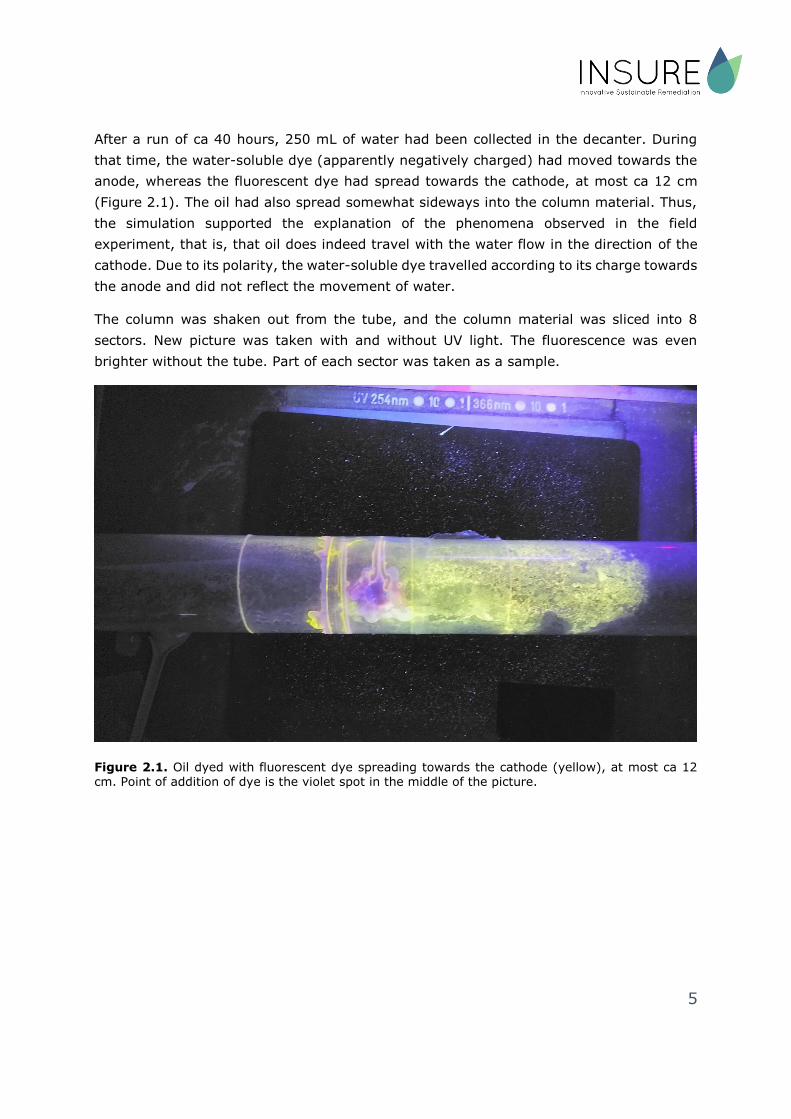
After a run of ca 40 hours, 250 mL of water had been collected in the decanter. During

that time, the water-soluble dye (apparently negatively charged) had moved towards the

anode, whereas the fluorescent dye had spread towards the cathode, at most ca 12 cm

(Figure 2.1). The oil had also spread somewhat sideways into the column material. Thus,

the simulation supported the explanation of the phenomena observed in the field

experiment, that is, that oil does indeed travel with the water flow in the direction of the

cathode. Due to its polarity, the water-soluble dye travelled according to its charge towards

the anode and did not reflect the movement of water.

The column was shaken out from the tube, and the column material was sliced into 8

sectors. New picture was taken with and without UV light. The fluorescence was even

brighter without the tube. Part of each sector was taken as a sample.

Figure 2.1. Oil dyed with fluorescent dye spreading towards the cathode (yellow), at most ca 12 cm. Point of addition of dye is the violet spot in the middle of the picture.

6

2.2. Tests using soil from Motala

A rectangular box was filled with oil-contaminated soil samples from the Motala site. Thin

plastic hoses were attached to the holes at the both ends of the vessel, near the soil

surface, to collect any water accumulated on the cathode side. The anode side was used

as a control.

Fluorescein (1 g of dye, 15 ml of water) and diesel dyed with oil-soluble dye were absorbed

into sawdust, which was added a few centimeters below the soil, in the middle of the vessel

(25 cm from the ends). The soil was then irrigated with 2 mM phosphate buffer, with a

volume of about 900 ml. The system was left to become soaked with water for a weekend.

The experimental setup (electricity connected) is shown in Figure 2.2.

After the weekend, the soil had sunk a few centimeters, resulting in the holes in the top

being exposed. Thus, new holes were drilled below the surface. Then the soil was examined

under UV light. Fluorescein had slightly spread while the oil dye was approximately in the

same shape and size as it was in the start of the experiment (Figure 2.3). The height of

the contamination was about 5 cm and its length was 10 cm; 4 cm towards the anode and

six cm towards the cathode. Less movement occurred vertically, however, dyed oil could

be observed to move downwards and slightly upwards.

In addition, about 100 ml of water was accumulated in a beaker on the cathode side. This

water was poured out and the test vessel was straightened with a spirit level. Electricity

was connected in the afternoon, and with 20 V, five mA electric current was formed. One

hour later, the electric current had remained unchanged, and about 50 ml of water had

accumulated in a beaker on the cathode side. The next day, about 50 ml of water was still

on the cathode side. Artificial pollution had spread in both directions; about 7 cm towards

the anode and about 10 cm towards the cathode. In addition, small amounts of dyed oil

were detected on top of the soil (Figure 2.4). 50 ml of water was added to the vessel evenly

using a pipette to compensate the loss of water.

During the next three days, no significant changes in location of the contaminant were

detected. Water was still accumulating on the cathode side and a total 100 ml of water

was added. The experiment was finished after four days. At the end of the experiment, pH

was measured using pH strips. On the anode side, pH was decreased to 3 while on the

cathode pH was 9. Fluorescein was observed to have disappeared almost completely from

the soil; small amounts were observed in water layer on the soil. Larger amounts of were

found in beakers, particularly on the cathode side (Figure 2.5).

7

About 1.5 weeks later, the test was re-started. 900 ml of water was added to the vessel

to soak the dry parts of the soil. When the soil was completely soaked, electricity was

turned on. At 20 V, five mA electric current was again produced. Before reconnecting the

electricity, the dimensions of the contamination were 19 cm at its widest and 12 cm at its

highest (ca 3 cm up, 9 cm downwards). Over the next two days, there was no significant

change in these dimensions. As in the previous experiment, water was accumulated on the

cathode side, this time in volume of only about 5 ml. The extent of the contamination at

the end of the experiment is shown in Figure 2.6.

Figure 2.2. An experimental setup of laboratory modeling. On the left is the anode side and on the

right is the cathode side.

8

Figure 2.3. Situation before switching on the electric current - the greenish water-soluble color

had started to spread, whereas the oil color had mainly remained in place. The injection spot is marked with the red circle.

9

Figure 2.4. A day after the connection of electricity, the artificial pollution was found to have spread in both directions; about 7 cm towards the anode and about 10 cm towards the cathode. The injection spot is marked with the red circle. Small amounts of dyed oil can be seen on top of the soil.

10

Figure 2.5. During the experiment, more water was accumulated on the cathode side (on the

right) and the color of it was more fluorescent than the color of water accumulated on the anode

side (left).

11

Figure 2.6. The situation after the end of experiment. The maximum width of the contaminated zone was 19 cm and the height was 12 cm. The injection spot is marked with the red circle.

2.3. Tests utilizing artificial soil

The experiment was performed in a smaller vessel (length 18 cm, height 19 cm, width 0.7

cm). A mixture of superfine clay type quartz sand and natural sand, in 50:50 ratio, was

used as the soil. Water was added to the vessel with a pipette so that the soil was wet

throughout. In the center of the vessel, over 5 cm below the surface, dyed sawdust was

added. The same dyes were used as in the previous experiment.

12

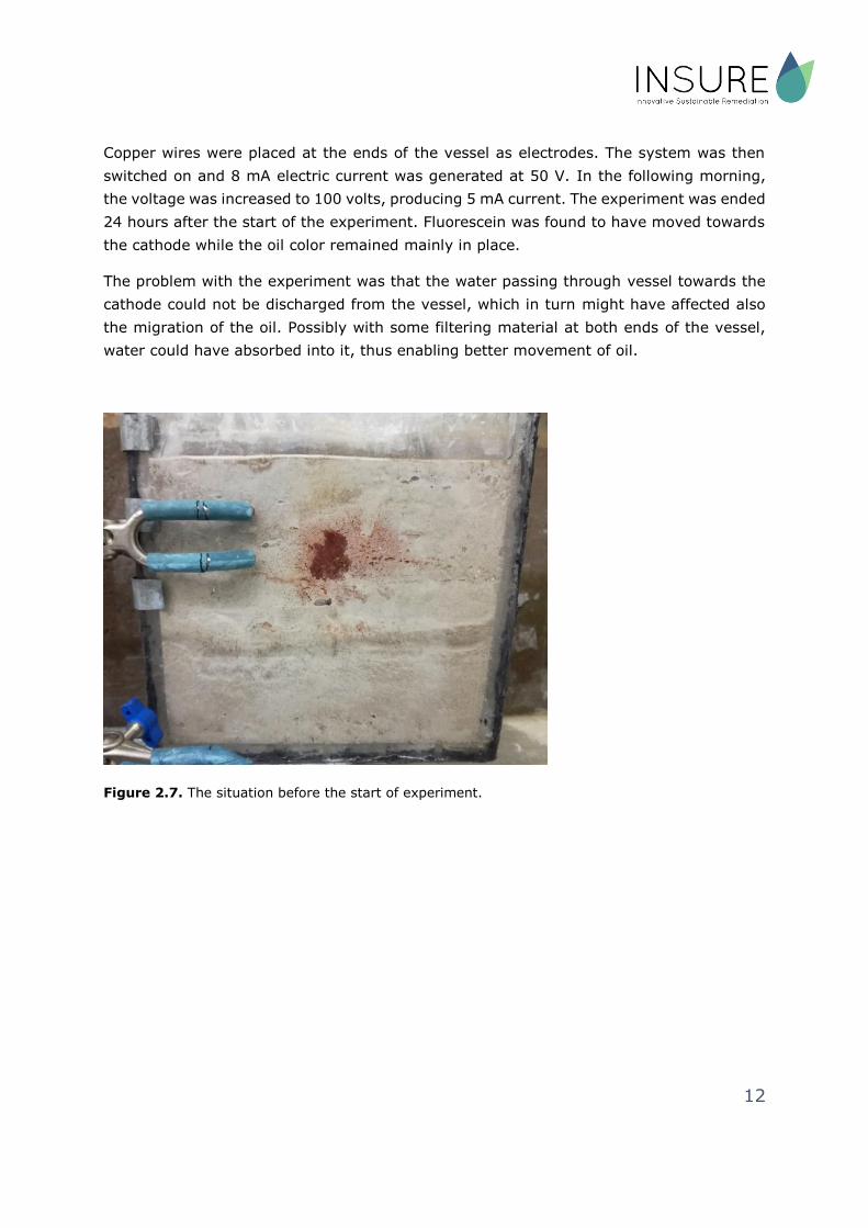
Copper wires were placed at the ends of the vessel as electrodes. The system was then

switched on and 8 mA electric current was generated at 50 V. In the following morning,

the voltage was increased to 100 volts, producing 5 mA current. The experiment was ended

24 hours after the start of the experiment. Fluorescein was found to have moved towards

the cathode while the oil color remained mainly in place.

The problem with the experiment was that the water passing through vessel towards the

cathode could not be discharged from the vessel, which in turn might have affected also

the migration of the oil. Possibly with some filtering material at both ends of the vessel,

water could have absorbed into it, thus enabling better movement of oil.

Figure 2.7. The situation before the start of experiment.

13

Figure 2.8. The situation immediately after switching on the electricity. The water-soluble

fluorescein (yellow color) had migrated towards the surface. The spreading before electricity has been marked with a black dashed line.

Figure 2.9. The situation about an hour after switching on the electricity. Fluorescein had moved towards the cathode, while the oil (red) had remained mainly in place, except for the right (anode) end, where the red color is slightly reduced.

14

Figure 2.10. Situation after about 24 hours. Fluorescein has clearly moved towards the cathode, while the oil contamination has still remained in place.

15

3. CHEMICAL OXIDATION

3.1. Lab-scale tests

In remediation hydrogen peroxide (H2O2) can be utilized as a chemical oxidant that

degrades organic compounds through the so-called Fenton’s reaction or rather, string of

reactions. In this reaction the breakdown of hydrogen peroxide is catalyzed by iron salt or

mineral iron in the soil, and reactive radicals are formed. For the radical producing reaction

to happen in sufficient efficiency, iron needs to be dissolved in the aqueous phase, and this

condition is only met in acidic pH. The pH range in which the catalytic iron in soluble in

water can however be expanded by adding chelating agents such as citrate into the soil.

Regardless of the reaction route, breakdown of H2O2 in water or soil may increase

volatilization of volatile contaminants, which should mean that H2O2 could be utilized as a

physical form of remediation for these particular compounds. Whether the primary reaction

mechanism is chemical or physical may play a minor role in cases when vapors are able to

exit the non-saturated soil, and when only volatile compounds are present. On the other

hand, if also non-volatile fractions are present, which is often the case, treatment through

the physical mechanism cannot be seen as the optimal solution.

In several laboratory and lysimeter scale studies, it was determined whether chemico-

physical H2O2 treatment would be a sufficient method for removal of VOCs from the

groundwater, and how non-volatile fractions of diesel would react in similar circumstances.

In addition, the effect of chelating citrate on chemical oxidation of aged diesel

contaminated soil was studied in the lysimeter scale.

16

3.1.1. Laboratory scale tests with

natural waters received from Nastola

and Motala.

A water sample from Nastola from an area contaminated with gasoline and a sample from

Motala from underneath a chemical cleaning facility, with high concentration of tri-chloro

ethylene, were used for testing the applicability of the H2O2 method on VOCs in the aqueous

media trapped in the pore space of soil.

Dry quartz sand was weighed into decanter glasses with 20 M of Fe(III)sulfate added as

the catalyst and the water was then added. The ratio between water and solid phases was

the same in both tests, whereas the volumes themselves differed (2 l / 10 l in the gasoline

test 1.2 l to 6 l in the TCE test). The effect of a 2 M dose of H2O2 on contaminant removal

was compared to that in a control treatment with only the water added. With the gasoline

contaminated water, also H2O2 concentrations of 0.5 M and 1 M were tested, and the water

also when appearing as a free water phase. In each case samples were withdrawn after

20+ hours since the H2O2 addition, when the reaction had waned and no gas was being

produced.

All samples were analysed at Eurofins according to the standard methods mod. ISO 11423-

1 and mod. EN ISO 10301 utilizing HS/GC/MS.

3.1.2. Results

Results indicated a successful removal of the contaminant for all gasoline components

already with a 0.4 M dose of H2O2 (Table 3.1). Due to the higher contamination level in the

Motala water, end concentrations for trichloroethylene were still above LOQ-level with the

full 2 M dose of peroxide. In general, it was found that the method was applicable for a

wide range of VOCs, regardless of their molecular weight. According to these results,

similar method would in principle be applicable for both sites in question.

17

Table 3.1 Results from the tests with natural water samples from Nastola and Motala.

Trichloroethylene was the sole component present in the Motala samples, listed last under

the category of halogenated compounds.

3.2.1. VOC composition test

The validity of the PID-method was tested with methyl tetra butyl ether (MTBE) spiked

pore water,. MTBE was chosen as the target compound because of its environmental

relevance but also because of its high water solubility and therefore, low amount of the

contaminant appearing as non-aqueous phase liquid (NAPL).

To detect whether contaminant removal was primarily happening through volatilization

rather than chemical oxidation, concentrations of MTBE, as well as its possible chemical

breakdown products, both in the gaseous and the aqueous phases were monitored.

original

0 M 0,4 M 1 M 2 M 0 M 2 M

compound

Aromatic benzene 2 4 <0,1 <0,1 <0,1 1 <0,1

toluene 130 250 <1 <1 <1 69 <1

Ethylbenzene 79 120 <0,1 <0,1 <0,1 3 <0,1

m+p-xylene 130 230 <0,1 <0,1 <0,1 170 <0,1

o-xyleeni 120 200 <0,1 <0,1 <0,1 140 <0,1

n-propylbenzene <0,1 0,3 <0,1 <0,1 <0,1 <0,1 <0,1

isopropylbenzene 0,2 0,2 <0,1 <0,1 <0,1 <0,1 <0,1

2-ethyltoluene 10 14 <0,1 <0,1 <0,1 10 <0,1

3-ethyltoluene 10 15 <0,1 <0,1 <0,1 12 <0,1

4-ethyltoluene 7 11 <0,1 <0,1 <0,1 7 <0,1

1,2,3-trimethylbenzene 8 12 <0,1 <0,1 <0,1 10 <0,1

1,3,5-trimethylbenzene 1 13 <0,1 <0,1 <0,1 8 <0,1

1,2,3,5-tetramethylbenzene 2 3 <0,1 <0,1 <0,1 2 <0,1

1,2,4,5-tetramethylbenzene 1 2 <0,1 <0,1 <0,1 1 <0,1

naphtalene 2 3 <0,5 <0,5 <0,5 5 <0,5

Ethers

MTBE 2 3 <0,1 <0,1 <0,1 3 <0,1

TAME 1 1 <0,1 <0,1 <0,1 0,6 <0,1

Aliphatic

2-methylpentane 4 4 <1 <1 <1 2 <1

3-methylpentane 3 3 <1 <1 <1 <1 <1

methyl-cyklopentane 2 3 <0,5 <0,5 <0,5 1 <0,5

cyclohexane 1 2 <0,5 <0,5 <0,5 0,7 <0,5

Halogenated 1,2-dibromoethane 1 1 <0,1 <0,1 <0,1 1 <0,1

original

0M 1 M

trichloroethylene 3700 310 2

c (µg/l)

c(H2O2) seperate water phase water in pore space

c(H2O2) seperate water phase water in pore space

c (µg/l )

18

The treatment with 5 M concentration of H2O2, both with and without the 20 mM

Fe(III)sulfate catalyst was compared with plain water control. Gaseous samples were

withdrawn 15 minutes, 60 minutes and 240 minutes after the peroxide injection. Absorbent

collector Anasorb 747, SKC 226-81A coupled with a Markes Acti-Voc pump was used for

this sampling. A different 20 liter PVP bucket was used for each measurement to limit the

transport of vapors. Water samples were withdrawn 20+ hours after the injection, due to

gas producing reactions still taking place after 240 minutes.

The absorbent sample and the water were analyzed at the accredited laboratory Eurofinns

according to standard methods ISO11423-1 and ISO20595. The absorbent collector was

analyzed gas chromatographically at the Finnish Institute of Occupational Health, with the

accredited method KEMIA-TY-006.

3.2.2. Results

The results indicated that the balance between reaction mechanisms was altered by

addition of catalyst in regards to breakdown products of MTBE, aceton and Tetra butyl

formate (TBF). This was likely because of the pH lowering effect of the catalyst addition.

With added catalyst, no peak in volatilization was detected, which would suggest that

reductions were related to the chemical mineralization occurring. These breakdown

products were also detected in higher doses than in the soil mineral catalysed treatment.

In the latter case volatilization couldn’t be ruled out either, but its role in the total removal

of MTBE was by comparison only moderate, as without the added catalyst heightened

volatilization was documented and found adding to the removal efficiency during the initial

stages (Table 3.2).

19

Table 3.2. Concentrations of MTBE and its breakdown products in the gaseous and

aqueous phases in the tested treatments. The percentage corresponding with MTBE

concentration in headspace relates to the mass added in the beginning.

ambient headspace water

C9-C11

time cyclical MTBE TBF Acetone MTBE Acetone

mg/m3 mg/m3 mg/m3 (μg/l) (mg/l)

5 M H2O2+ 15 min <0.3 120 (5%) 10 <1

20 mM Fe(III)SO4 60 min <0.3 94 (4%) 14 <1

240 min <0.3 1,8 (0,1%) 1.9 <1

>20 h <0.5 1.0

5 M H2O2 15 min <0.3 430 (18%) <0.6 <1

60 min <0.3 320 (13%) <0.6 <1

240 min <0.3 160 (7%) 1.6 <1

>20 h <0.3 7,6 (0,3%) 2.8 1,9 8.8 1.8

Control 15 min 0 160 (7%) <0.6 <1

60 min 0 240 (10%) <0.6 <1

240 min 2.9 290 (12%) <0.6 <1

>20 h 7700 <0.05

These results indicate that in the previous test, chemical mineralization had been the

primary reduction mechanism. The situation would therefore be somewhat different on

field, where additional catalysts would not be added and the soil pH would in most cases

be closer to neutral. With positive results also from the test without added catalyst, natural

soil pH treatment would still allow for considerable reductions of volatile contaminants, and

in these cases the total effect would be achieved by combination of both the chemical and

physical removal mechanisms.

20

3.3.1 MTBE spiked water lysimeter

test

Pilot-scale tests for MTBE contaminated water was performed in 2m2 metal lysimeters at

SOILIA field research station. Water spiked with MTBE (750 mg/l) was treated as a

separate water phase and also as pore water withheld in a 1m3 column of soil (Figure 3.1.).

In the free water phase test water was poured into the lysimeters, after which the MTBE,

and then the H2O2 and was added in 1 M H2O2 concentration. In the control study, the

volume of peroxide was compensated by a corresponding volume of water. The total

volume of the aqueous phase was 400 l. Fe(III) in concentration 2 mM to total volume was

used as the catalyst.

Samples were taken by bucket every 24 hours until peroxide concentration was measured

to have fell below 0.0%. PID values and temperatures were recorded at the time of each

sampling. During the first hours after the addition, the on-going reaction prevented

samples from being analyzed. H2O2H2O2

Citrate

1) H2O2 (1M)

2) H2O2 (2M)

3) H2O2 (2M)

1) control

2) control

3) H2O2 (2M)

Fe(II) (0,02 M)

H2O2

Citrate

Fe(II)Control

ControlH2O2 (1M)

Fe(III) (2 mM)

MTBE-spiked water in pore space

MTBE-spiked water

Aged diesel contaminated soil in water

Figure 3.1. The test setup for the MTBE spiked water treatment in free water and pore

water phases.

In the soil experiment MTBE spiked water was poured into the soil columns, with or without

peroxide. Water samples were withdrawn from the bottom valves of the lysimeters and

PID values and soil temperature were measured from 0.5-1 m deep holes in the soil

column. As with the water experiment, samples with viable gas forming were not analyzed.

21

The experiment consisted of three steps (Figure 3.1). During the first step H2O2 was added

in concentration 1 M per total aqueous phase volume, of which 50 % was in the soil

originally, the concentration thus corresponding with that in the free water phase

experiment. During the next two steps peroxide concentration was doubled to 2 M to total

volume. The total aqueous phase volume increased after each step by 40 liters of further

peroxide and corresponding H2O2 additions and also new MTBE was therefore added. After

two steps the addition of H2O2 in concentration of 2 M to total volume was repeated, while

the control treatment was replaced with a test with similar peroxide addition but with an

additional iron(II) catalyst added in dose 20 mM . At the closure of these experiments,

after the water phase had been removed, the soil column was sampled in four vertical sub-

samples for VOC analysis for verifying that the system was in balance.

3.3.2 Results

Results from both the free water phase experiment and pore water experiment in lysimeter

scale indicated successful removal of the contaminant, but also significant differences

across the two medias (Figure 3.2 a & b.). Lower efficiency for soil bound contaminant was

to be expected according to both literature and technology providers. Also, since additional

catalyst was used in the water experiment, pH was adjusted to a level more optimal for

chemical mineralization.

In the lysimeter experiment H2O2 addition of 2 M led to 31% reduction in MTBE

concentration compared with the concentration in the control treatment at same date. Only

50% of the added MTBE could be detected in the aqueous phase of the control lysimeter,

which means that large portion of the MTBE was volatized already during injection.

Repeated injection with 4 M dose resulted in further 90% reduction in MTBE concentrations,

totaling now 98% reduction from the concentrations in the control treatment. Another

injection in similar 4 M dose led to further 66 % reduction after a follow up period.

Addition of chelate was found successful in the sense that the resulting 88% drop in MTBE

concentrations during the day was the highest recorder decline during the experiment. In

this case reaction intensity was still found to have been too high as no peroxide was

detected at the bottom of the lysimeter.

Initial drops in concentrations were in all cases followed by rebounds in concentration.

Their relative size was found to increase with the concentrations in the aqueous phase

decreasing. Similar type of rebounds are associated with air sparging techniques, and are

caused by the returning concentration balance between the two medias, air and water. The

effect of the rebounds on the total reductions was still relatively low.

22

Figure 3.2 a & b. Results from the free water phase experiment (a) and pore water

experiment (b). Non-continuous x-axis in figure 3.2 b. LOG10 transformed Y-axis in both

cases.

1

10

100

1000

10000

100000

1000000

0 1 2

c(MTBE)

log10(mg/l)

t (d)

1 mol H2O2+ 0,002 molFe(III)

control

23

3.4.1. Aged diesel contaminated soil

lysimeter test

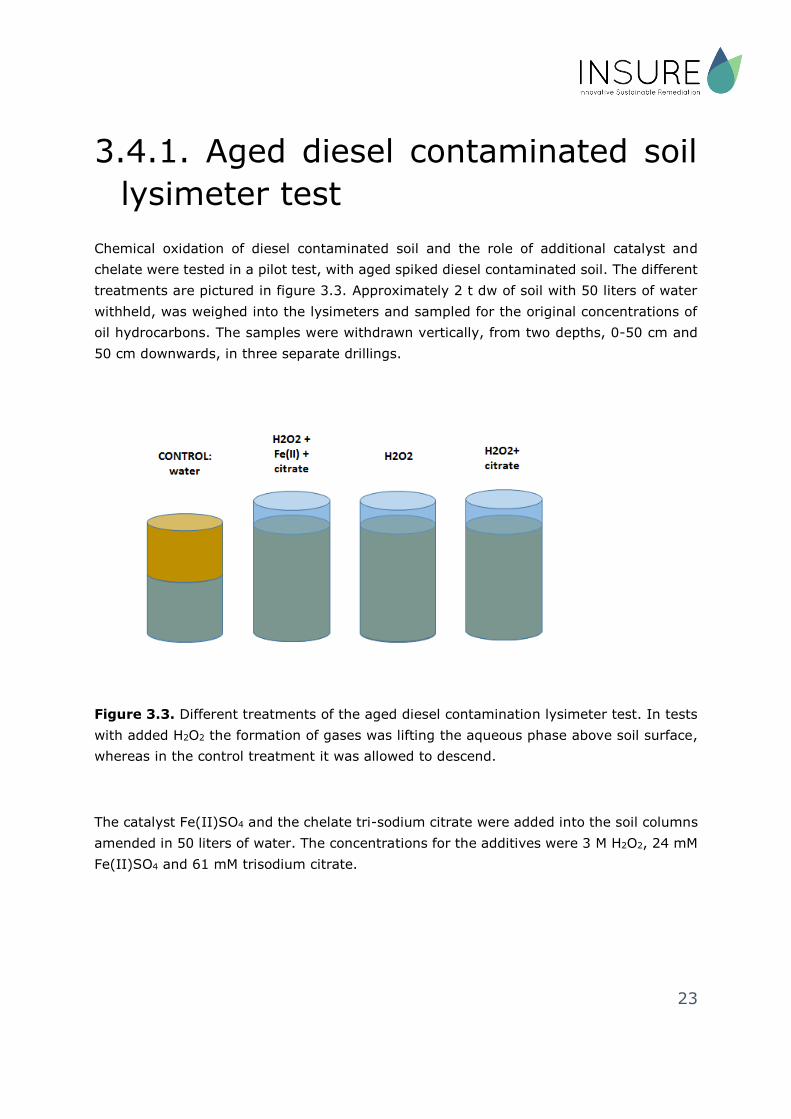
Chemical oxidation of diesel contaminated soil and the role of additional catalyst and

chelate were tested in a pilot test, with aged spiked diesel contaminated soil. The different

treatments are pictured in figure 3.3. Approximately 2 t dw of soil with 50 liters of water

withheld, was weighed into the lysimeters and sampled for the original concentrations of

oil hydrocarbons. The samples were withdrawn vertically, from two depths, 0-50 cm and

50 cm downwards, in three separate drillings.

Figure 3.3. Different treatments of the aged diesel contamination lysimeter test. In tests

with added H2O2 the formation of gases was lifting the aqueous phase above soil surface,

whereas in the control treatment it was allowed to descend.

The catalyst Fe(II)SO4 and the chelate tri-sodium citrate were added into the soil columns

amended in 50 liters of water. The concentrations for the additives were 3 M H2O2, 24 mM

Fe(II)SO4 and 61 mM trisodium citrate.

24

H2O2 additions were performed twice with a three week interval, once the peroxide

concentrations were under detection limits as measured with peroxide strips (Merck

peroxide test). Peroxide was added to the original total 3.1 M concentration, whereas

citrate and Fe(II)SO4 were diluted through this addition to a lower level.

While the H2O2 breakdown reaction was still ongoing, the sampling of both soil and water

could only be performed from the surface. Temperature was measured during each site

visit.

After the experiment was concluded, the soil column was sampled from depths 0-5 cm, 5-

50 cm, 50-100 cm and 100-150 cm, with three individual samples from each depth. Oil

hydrocarbons in soil were analyzed according to standard ISO 16703:2005 with HP 6890

Gas chromatography device with FI-Detector. Oil in water was analyzed according to

standard method SFS-EN ISO 9377-2 by Eurofins.

3.4.2 Results

For aged diesel contaminated soil, reductions in the 10% range were achieved for all

treatments with added H2O2, with no significant difference between the three test with

differing amounts of catalyst of chelate (Figure 3.3). The performance level for diesel

appeared hence relatively low, whereas the total mass of the contaminant in the soil far

exceeded the amount of MTBE in the corresponding test. This would mean that in terms

of H2O2: contaminant mass ratios, the differences to the MTBE tests were less critical.

Figure 3.3. Diesel contaminated soil lysimeter scale test results, average reductions ±

standard deviation. Reductions per original level are shown in numbers percent.

100

300

500

700

900

1100

1300

control H2O2 +Fe(II)+citrate

H2O2 H2O2 +citrate

c(C10-C40)

(mg/kg dw)reduction end concentration

0,5% 13,5% 12,7% 15,4%

25

Both in the lysimeter test and small scale tests modelling the same phenomena, oil was

found to accumulate to the soil surface as a result of the sparging effect. This

phenomenon is pictured in figure 3.4. Because of this vertical transport, the soil samples

withdrawn from the top soil during the treatment were not representative of the total oil

concentrations.

Figure 3.4. Addition of H2O2 into quartz sand spiked with red-dyed diesel. The reaction is

mobilizing the oil towards the soil surface.

The results indicate that chemical treatment of aged diesel contaminated soil would lead

to temporal mobilization of the contaminant, whereas with VOCs, this effect could be in

principle benefitted from. Due to the high total mass of the contaminant in soil in most

cases of diesel contamination, in comparison to water soluble VOCs, the former is more

difficult to treat as it would require higher amounts of H2O2. When the aforementioned

consequences of the physical mechanisms are taken into account, the two contaminants

are prone to act differently.

Both the suitability tests for areas contaminated with VOCs and the related field treatment

of site Loppi have been reported in a more thorough manner in the Master’s thesis of M.Sc.

Niina Lallukka, “VOC-yhdisteiden poistaminen pohjavedestä vetyperoksidin kuplitus –

menetelmällä” (In Finnish, with an abstract written in English) reported as a deliverable.

26

Both the laboratory and the lysimeter scale studies with MTBE contaminated water and

aged diesel contaminated soil have been used as a material for the article “Fenton’s

reaction based chemical oxidation in suboptimal pH conditions can lead to mobilization of

oil hydrocarbons but also contribute to the total removal of volatile compounds” submitted

to the Journal “Environmental Science and Pollution Research” in June 6th 2019. This article

will be made available through open-access once accepted for publication.

4. BIOFLUSHING

4.1. Methyl-β-cyclodextrin laboratory

scale test

In some biostimulation treatments, the primary bottleneck for biological degradation is the

low bioavailability of the contaminant hydrocarbons. Low bioavailability is the desired state

when only environmental risks are being considered, but without removing this bottleneck,

biostimulation efforts can be ineffective. In these cases soaps can be introduced to help

dissolve the compounds with low bioavailability. Biodegradable soaps are preferred

whereas products with high biodegradability tend to inhibit the degradation of the

contaminant by acting as more readily available carbon sources than the contaminant

itself. Also the total dose of the soap need to regulated, so that the oil hydrocarbons are

being released into the aqueous phase in sufficient doses for them to be degraded before

being spread into groundwater or outside the contaminated zone.

Methyl-β-cyclodextrin (CD) has been chosen as the optimal surfactant based on results

from former studies. Cyclodextrin is procuded from a raw material containing strach. It is

a cyclical sugar that binds the hydrophobic target compound in its hydrophobic inner

circumference with Van der Waals interaction and thus dissolves it in water due to the

hydrofilic outer circumference of the forming complex. CD itself is biodegradable but not

to the extent where is would act as a more readily available source of organic carbon.

27

The effect of CD on the removal of oil hydrocarbons was tested in a laboratory scale test

with soil withdrawn from site Karjaa. At the site the contaminated zone had been treated

with bioflushing for several years, the most recent results suggesting that the water soluble

fractions had successfully degraded. After the remediation steps already performed, the

highest measured C10-C40 concentration detected has been 1500 mg/kg, found to consist

almost entirely of aliphatic compounds in the C12-C15 and C16-C21 ranges.

In the laboratory test, soil samples taken from the site were mixed with the treatment

solution (200 g of soil, 300 ml of solution). Three different treatments were tested: 5 %

and 1 % (v:v) (CD) and water control. During the first step, bottles were shaken in 1-hour

cycles, five times altogether. Phases were allowed to separate between each shaking.

During the second time, the experiment was repeated in a similar manner but with 5-hour

shaking periods. The water phase was sampled after each step. Since the soil was

completely water saturated, the results are not reflective of a situation where the solvent

is merely filtrated through the soil column. With the tests it was however possible to see

to which degree the solubility of a particular fraction range can be increased in an optimal

situation. All treatments were performed as three replicas, with one of these per treatment

randomly selected for fraction analysis. The two remaining replicas were tested only for

fraction sums C10-C40, C10-C21 and C21-C40.

4.2. Results

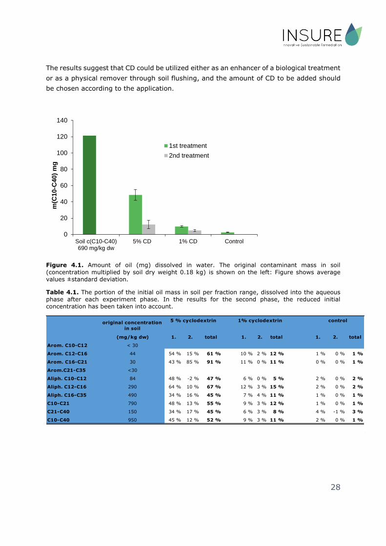
Based on the results, the amount of CD positively affected the hydrocarbon concentrations

in the aqueous phase. The mean concentrations from the different treatments differed at

both sampling times for all measured oil hydrocarbon groups (C10-C40, C10-C21 and C21-

C40) (Figure 4.1). The added benefits concern specific fractions differently, as the

efficiency remained particularly high for the C16-C21 range aromatic compounds (Table

4.1). For C10-C12 aliphatic compounds, the final removal rate (48%) was achieved already

during the initial shakings. In addition, it was found that the efficiency was dependent on

the CD concentration rather than the total dose as by using 1% CD concentration, final

results were achieved within similar period as when 5 % CD concentration was used,

whereas the efficiency itself was still weaker. The same phenomenon appeared to concern

other fractions as well, but to a lesser extent.

28

The results suggest that CD could be utilized either as an enhancer of a biological treatment

or as a physical remover through soil flushing, and the amount of CD to be added should

be chosen according to the application.

Figure 4.1. Amount of oil (mg) dissolved in water. The original contaminant mass in soil

(concentration multiplied by soil dry weight 0.18 kg) is shown on the left: Figure shows average values ±standard deviation.

Table 4.1. The portion of the initial oil mass in soil per fraction range, dissolved into the aqueous phase after each experiment phase. In the results for the second phase, the reduced initial concentration has been taken into account.

0

20

40

60

80

100

120

140

Soil c(C10-C40)690 mg/kg dw

5% CD 1% CD Control

m(C

10-C

40)

mg

1st treatment

2nd treatment

(mg/kg dw) 1. 2. total 1. 2. total 1. 2. total

Arom. C10-C12 < 30

Arom. C12-C16 44 54 % 15 % 61 % 10 % 2 % 12 % 1 % 0 % 1 %

Arom. C16-C21 30 43 % 85 % 91 % 11 % 0 % 11 % 0 % 0 % 1 %

Arom.C21-C35 <30

Aliph. C10-C12 84 48 % -2 % 47 % 6 % 0 % 5 % 2 % 0 % 2 %

Aliph. C12-C16 290 64 % 10 % 67 % 12 % 3 % 15 % 2 % 0 % 2 %

Aliph. C16-C35 490 34 % 16 % 45 % 7 % 4 % 11 % 1 % 0 % 1 %

C10-C21 790 48 % 13 % 55 % 9 % 3 % 12 % 1 % 0 % 1 %

C21-C40 150 34 % 17 % 45 % 6 % 3 % 8 % 4 % -1 % 3 %

C10-C40 950 45 % 12 % 52 % 9 % 3 % 11 % 2 % 0 % 1 %

original concentration

in soil

5 % cyclodextrin 1% cyclodextrin control