REPLACEM ENT INVESTM ENT: OPTIM AL ECONOM IC LIFE UNDER UNCERTAINTY

by

Ian M . Dobbs*

Department of Accounting and Finance, and Newcastle School of Management University of Newcastle upon Tyne, NE1 7RU, England.

K EYWORDS: Capital Budgeting, Economic L ife, I tô processes, Option Value. JEL CLASSIFICATION: G31

4

ABSTRACT

Replacement investment is essentially a regenerative optimal stopping problem; that

is, the key decision concerns when to terminate the life of existing plant – and hence

when to start over again. This paper examines this optimisation problem within a

continuous time framework and studies the qualitative and quantitative impact of

uncertainty on the timing of new investment (and the criteria that should be used for

terminating the life of existing plant).

1

1. INTRODUCTION

A large part of all investment activity is in fact replacement investment; indeed in a

non-growing, stationary state, economy, effectively all investment is replacement

investment. The key decision concerning such replacement investment is that of

timing – of deciding how long to keep existing plant and machinery. As an

optimisation problem, the decision of when to renew capacity naturally depends on

expectations regarding how existing and new plant operating costs change over time,

and of course, on expectations regarding future capital costs and resale/salvage

values. A standard approach is to envisage a replacement chain for investment in

which the economic life of the first plant is determined by a trade off between

expected benefits and costs associated with extending the economic life of existing

plant. Keeping plant for an additional period involves incurring additional operating

costs and suffering possible loss of second hand or salvage value, but reduces the

present value costs associated with the chain of investments that subsequently follow.

The analysis of replacement investment in this framework has been around for a

considerable time and is well understood (for early examples, see e.g. Hotelling

[1925], Terborgh [1949], McDowell [1960], Smith [1961], Merrett and Sykes

[1965]).

Replacement investment under uncertainty has also been examined, notably in the

Operational Research literature (for reviews, see Pierskalla and Voelker [1976],

Sherif and Smith [1981]). This literature primarily focuses on uncertainty over the

physical life of individual components, with the problem being viewed as one of

determining a replacement policy, where such a policy will typically involve

2

replacing at least some units before the end of their physical life.1 Optimal economic

life may also depend on second hand (or salvage) values, and so a natural extension to

the study of investment policy is to look at replacement investment within the context

of equilibrium in the associated second hand markets (Rust [1985]). More recent

work has tended to focus on other aspects of the replacement problem, notably how

asymmetric information affects equilibrium values in second hand markets (following

the seminal work of Akerlof [1960], see Kim [1985], Genesove [1995]).

The above literature has generally modelled the replacement investment decision

within a discrete time framework; by contrast, the present paper begins by modelling

the optimisation problem in a continuous time framework (and focusing on the

‘option value’ characteristics of the solution). Following this, the paper examines in

some detail the qualitative and quantitative impact of uncertainty (and other

parameters) on the replacement decision and on the average economic life of plant.

Previous work does not seem to have examined this type of comparative statics

analysis of the investment decision; broadly speaking, the OR literature has tended to

feature rather case specific models, with the focus on establishing the existence of a

‘solution’ , whilst the economics literature has tended to focus on the issue of

characterising ‘equilibria’ in second hand markets without pursuing the further

question of how such equilibria are perturbed by variation in the underlying parameter

values. The equations that characterise the solution to the replacement investment

decision are used in this paper as the basis for undertaking sensitivity analysis and the

study of alternative ‘scenarios’ .

1 Rust [1987] is perhaps one of the best examples of this type of analysis – that paper examined the optimal replacement policy for replacing/rebuilding Bus engines, given the probability that such engines break down is a function of mileage.

3

In the context of the replacement chain investment, uncertainty creates option value.

If the objective is to minimise expected present value costs, the decision to terminate

the life of existing plant should take account of the possibility that operating and

maintenance costs can go down as well as up. Dixit [1989] has shown that

competitive firms, when faced with uncertainty over market price, do not exit the

industry immediately price falls below average variable cost; price has to fall

somewhat further; the same type of effect can be expected in the present context,

namely that uncertainty can be expected to extend the economic life of plant (and

within the context of the present model, it is possible to prove this result).

The present paper assumes there is a fixed and time invariant salvage value. The

assumption regarding second-hand markets is either that (a) they do not exist, such

that the decision is always one of replacing the old plant with new, or (b) that there is

no information asymmetry and no transactions costs, such that the market price of

second hand equipment represents a fair and competitive value. This latter

assumption is often reasonable in quite a range of applications; asymmetric

information may be of importance in used car markets, but such severe forms of

asymmetric information are far from endemic.

If there is no second-hand market, clearly the firm must take the decision on when to

replace existing with new plant. By contrast, with competitive second-hand markets,

whilst the economic life of the plant remains the same as in the case where there is no

second hand market, the decision of the individual firm (as to what age of plant to

buy, and of when to sell) becomes a matter of indifference (it makes no difference

4

how old the plant bought is, or indeed when it is sold, so long as it is not kept beyond

the time at which it would have been better to scrap it). In this latter case, it is also of

interest to study the time profile for second-hand values.

The structure of the paper is as follows: Section 2 first establishes the basic model.

Following this, section 3 focuses on economic life and second hand values whilst

section 4 discusses alternative measures of economic life. Section 5 establishes some

comparative statics results and conducts a (numerical) sensitivity analysis; section 6

then offers some concluding comments on the relevance of the work and direction for

further research.

2. REPLACEM ENT CHAINS UNDER UNCERTAINTY

In what follows, the solution for the deterministic case is outlined as a preliminary

benchmark, prior to extending the analysis to incorporate uncertainty regarding

operating costs and resale values. As explained in section 1, whether or not there are

competitive second-hand markets, it suffices to analyse the economic life of plant per

se. In the case where there are (competitive) second hand markets, equilibrium

second hand values for plant can then be computed.

The Deterministic Case

The initial capital outlay is denoted K, operating/maintenance costs at time t are tc

and are assumed to increase at a constant growth rate θ whilst salvage value S is

assumed constant. Let V denote the present value of all costs associated with a

replacement chain, and assume that the first plant is terminated at some time T. The

big assumption in replacement chain analysis is that the initial outlay and operating

5

cost profiles for the second and subsequent plant do not change. Under this

‘stationarity’ assumption, it follows that T is the optimal economic life for each and

every plant in the replacement chain. Thus, V also represents the present value at time

T of all future costs from T onward. Hence

( ) ( )0

Trt rT

tV K c e dt V S e− −= + + −�

, (1)

where r denotes the risk free discount rate (assumed constant over time). The first

term on the right hand side is the initial capital outlay, the second term represents the

present value of operating costs for the first plant whilst the third term represents the

present value of selling the old plant for its salvage value S and then starting the chain

anew (with present value cost V at that time). Rearranging (1), the present value of

costs can be represented as the function

( )( )00

1( , , , , , ) 1

1r T rT

rT

cV T r c K S e K Se

e rθθ

θ− −

− � �= − + −� �

− −� � . (2)

Optimal economic life, certT is thus given as

, 0 0Argmin ( , , , , , )cert T TT V T r c K Sθ>= , (3)

whilst the associated level of operating cost, denoted certc , at which replacement

investment is triggered is

0certT

certc c eθ= (4)

(this proves of interest when making comparisons with the uncertainty case). The

function (2) is non-linear but the optimisation can easily be conducted using

numerical methods.2 The quantitative sensitivity of the above certainty solution to

2 It is possible to compute a first order condition associated with (2), but this in turn does not admit an

explicit solution for certT ; the only gain from computing such a first order condition is that it is then

possible to conduct a comparative statics exercise. This is in fact a special case of the more general comparative statics exercise presented for the uncertainty case in section 4 below.

6

changes in parameter values is examined at the same time as that for the uncertainty

case in section 4 below.

Optimal Economic L ife under Uncertainty

Terborgh [1949] was one of the first to model operating costs (under certainty) as

increasing by a constant percentage increment; this type of assumption is both

empirically plausible and also analytically fairly tractable. The natural extension is to

assume that uncertainty affects the level of operating costs, tc through a geometric

Brownian motion (GBM) of the form3

/t t tdc c dt dθ σ ϖ= + . . (5)

Here θ (>0) is the trend rate of growth in operating cost and σ (>0) denotes its

associated volatility. When σ =0, of course, this is the original ‘Terborghian’

operating cost process. The expected present value of operating costs at time τ , if the

operating cost at this time is cτ , for the case where the plant is never replaced is given

as

( ){ }( ) r ttPV c E c e dtτ

τ τ τ τ

∞ − −= � , (6)

where (.)Eτ denotes the expectations operator for expectation formed at time τ .

When operating costs rise sufficiently, it becomes economic for plant to be replaced.

Let c denote the level of cost at which replacement is triggered. Given the structure

of the problem and the assumptions regarding the cost process, c is a fixed

deterministic value. The optimisation problem is simply that of finding the value c

3 GBM is a common assumption in the literature. For a discussion of its pros and cons, see McDonald and Siegel [1986] and Dixit and Pindyck [1994].

7

which minimises expected present value costs for the replacement chain (clearly, c

will be a deterministic function of the parameters 20, , , , ,K S c rθ σ ). By contrast, since

the evolution of cost over time is governed by an Itô process, the time at which

replacement is triggered is a random variable, ( )t c�

(to denote its dependence on c ).

The present value of future costs, for the existing plant, thus depends on the current

operating cost level, such that, at time τ during the life of the first plant, the expected

present value of future operating costs for the chain can be written as

( )( ) ( ) ( ( ) )( ) ( )t c

r t r t ctV c E c e dt e W c

τ

τ ττ τ

− − − −= +��� �

, (7)

where ( )W c represents the present value at time ( )t c�

of all costs from that time

onward; that is

0( ) ( )W c V c K S= + − . (8)

In what follows, for notational compactness, subscripts and arguments are dropped

wherever this does not affect intelligibility. The arbitrage condition for this problem

is that4

( )rVdt cdt E dV= + . (9)

The term ( )E dV is evaluated in the appendix. It can be written as5

2 212( )E dV V cdt V c dtθ σ′ ′′= + , (10)

and so (9) simplifies to give (cancelling through by dt)

2 212 0c V cV rV cσ θ′′ ′+ − + = , (11)

a second order differential equation which governs the evolution of value. The

general solution to this equation involves finding a particular solution to it along with

4 See e.g. Dixit and Pindyck [1994] for a clear exposition of stochastic dynamic programming optimality conditions. 5 Using the notation 2 2/ , /V dV dc V d V dc′ ′′≡ ≡ .

8

a general solution to the associated homogenous equation. A particular solution,

(assuming r θ≠ ) is /( )V c r θ= − as can be easily verified.6 The general solution to

the homogenous equation can be written as 1 21 2( )V c Ac A cλ λ= + (see appendix) and so

the general solution to (11) can be written as

( )( ) 1 21 2( ) /V c c r Ac A cλ λθ= − + + , (12)

where the roots are defined as

( ) 21 1 2 /R Rλ σ= − + , (13)

( ) 22 1 2 /R Rλ σ= − − , (14)

and where

( )211 2R θ σ≡ − , (15)

( )1 22 22 1 2R R rσ≡ + . (16)

Notice that 22 0rσ > if 2 0σ > , so 2 10λ λ< < ; the roots are real and of opposite sign

when uncertainty is present. The two arbitrary constants 1 2,A A are determined by

boundary conditions. As 0c → , since 2 0λ < and since value must be finite, this

implies 2 0A = (Dixit [1993] discusses this sort of boundary condition in more

detail). Thus (12) simplifies to

( )( ) 11( ) /V c c r Acλθ= − + , (17)

where 1A is determined by an analysis of smooth pasting conditions at the boundary

where replacement investment takes place; these smooth pasting conditions require

6 To see this, note that if /( )V c r θ= − , then 1/( )V r θ′ = − and 0V ′′ = ; substitute these into (11).

9

equality of value and equality of the first derivatives (with respect to tc ) of the value

functions from regimes 1 and 2 (Dumas [1991]). Thus, at a hitting time t� , this entails

( ) ( )V c W c= , (18)

and

( ) / ( ) /V c c W c c∂ ∂ = ∂ ∂ . (19)

From (17), condition (18) becomes

( )( ) ( )( )1 11 0 0 1 0( ) / ( ) /V c c r Ac V c K c r Ac K Sλ λθ θ= − + = + = − + + − , (20)

whilst ( )( ) 1 11 1( ) / 1/V c c r A cλθ λ −∂ ∂ = − + , [ ]0( ) / ( ) / 0W c c V c K S c∂ ∂ = ∂ + − ∂ = , so

(19) gives

( )( ) 1 11 11/ 0r A cλθ λ −− + = . (21)

After some rearrangement, (20) and (21) give the solution

( ) ( )( ) ( )( )1

1 0 0 11 / 0c c c c K S rλλ θ λ

� �− − + + − − =� �

. (22)

This non-linear equation defines the level of operating cost c at which replacement

investment is triggered. In view of (13), (15), (16), the value of c is a function of

the parameters 0, , , , ,r c K Sθ σ . As in the deterministic case, an explicit analytic

expression for c cannot be obtained, although it is possible to obtain some qualitative

comparative statics result for the effects of parameters on the value of c and on

expected economic life. It is also straightforward to solve (22) numerically, and the

quantitative impact of parameter variations can be studied numerically. Section 4

presents these results. However, prior to this, section 3 examines economic life under

uncertainty.

10

3. ECONOM IC LIFE AND SECOND HAND VALUES

Under uncertainty, the economic life of a plant ( )t c�

is a random variable, and as a

consequence, economic life may turn out to be longer or shorter than in the

deterministic case. In what follows, we focus on the average or expected life of a

plant, ( )0 ( )E t c�

. An analytic expression for this expected life is extremely difficult to

obtain,7 but it is straightforward to derive a numerical approximation for it by running

a simple simulation model. The simulation model repeatedly generates paths for tc ;

for the thi run, it is possible to compute the time iT taken for tc to reach the trigger

level c . An estimator for ( )0 ( )E t c�

is thus given as

1

n

iiT T n

==

� (23)

if the simulation is run n times. In conducting this simulation, the operating cost

process can be approximated as a discrete process using the stochastic difference

equation8

( ) ( ) ( )211 2ln lnt t m m m tc c θ σ σ ε−= + − + (24)

where ~ (0,1)t Nε . Here, if σ represents an annualised value for volatility of the cost

process, then setting periods to months, such that 2 2 /12mσ σ= , and /12 1m eθθ = − ,

then ,m mσ θ represent the equivalent monthly rates for the variables ,σ θ .

7 Cox and Miller [1965, pp. 220-222] discuss the form of calculation required for a special case involving simple Brownian motion. In the more complex case involved in this paper, a closed form explicit solution cannot be obtained – getting a solution thus requires numerical methods at some point. 8 A Fortran program which runs this simulation is available from the author on request. The average economic life was computed for each case reported in the sensitivity analysis in section 4 below using

10,000N = runs.

11

An alternative and much simpler to calculate proxy measure for economic life,

denoted T̂ , involves calculating the time it takes for expected operating cost to reach

the level c . Thus, given that 0 0( ) ttE c c eθ= , this proxy measure is computed by

setting

ˆ

0 0ˆ (1/ ) ln( / )Tc e c T c cθ θ= � = (25)

This proxy under-estimates average economic life because the distribution for ( )t c�

is

skewed to the left. For low levels of volatility, the proxy is quite close to the estimate

of 0( ( ))E t c�

established using simulation but the quality of the approximation

deteriorates at higher volatilities (see next section).

In the case where there is secondary trading, it is possible to relate the selling price tp

of used equipment to the current level of operating cost it manifests, tc using the

value function (17). As previously remarked, given the competitive price, there is no

reason per se for a firm to wish to sell such equipment on such a market (since it is a

matter of indifference as to whether to sell or not, and for ongoing business, if plant is

sold, another plant of some age must also be bought). In a market with zero sunk

costs and no information asymmetries, the prime source of such equipment would

presumably be ‘distress’ stock; that is, equipment coming to market because firms

have ceased trading, or where there has been a fall in demand for their products. So

long as there is always some positive demand for replacement investment, second

hand prices will not be affected by product market fluctuations, and will be

determined solely by cost characteristics. From (17), using (21) to replace the

constant 1A , value can be written as

12

( )( )( )1 1

1( ) 1/ / 1c

V c c cr

λλθ

−���

= −���

−��� (26)

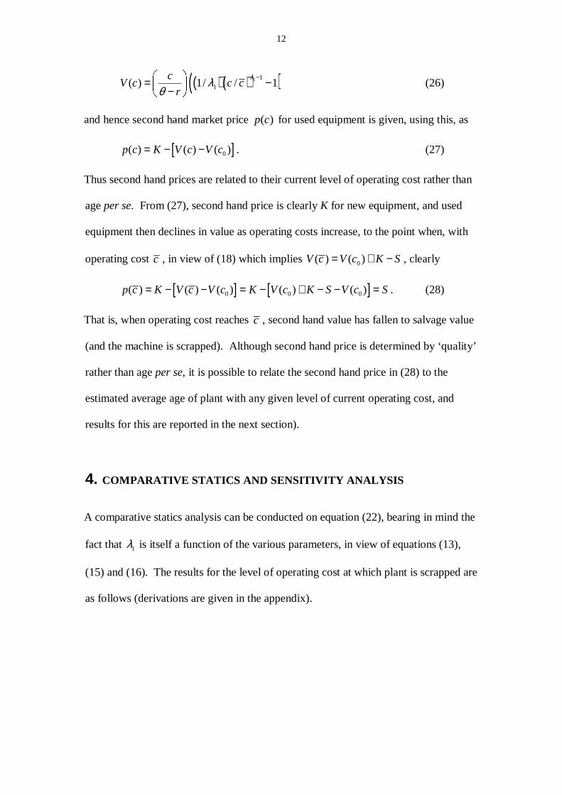
and hence second hand market price ( )p c for used equipment is given, using this, as

[ ]0( ) ( ) ( )p c K V c V c= − − . (27)

Thus second hand prices are related to their current level of operating cost rather than

age per se. From (27), second hand price is clearly K for new equipment, and used

equipment then declines in value as operating costs increase, to the point when, with

operating cost c , in view of (18) which implies 0( ) ( )V c V c K S= + − , clearly

[ ] [ ]0 0 0( ) ( ) ( ) ( ) ( )p c K V c V c K V c K S V c S= − − = − + − − = . (28)

That is, when operating cost reaches c , second hand value has fallen to salvage value

(and the machine is scrapped). Although second hand price is determined by ‘quality’

rather than age per se, it is possible to relate the second hand price in (28) to the

estimated average age of plant with any given level of current operating cost, and

results for this are reported in the next section).

4. COM PARATIVE STATICS AND SENSITIVITY ANALYSIS

A comparative statics analysis can be conducted on equation (22), bearing in mind the

fact that 1λ is itself a function of the various parameters, in view of equations (13),

(15) and (16). The results for the level of operating cost at which plant is scrapped are

as follows (derivations are given in the appendix).

13

Table 1: Comparative Statics Results

Parameter ψ /dc dψ

Capital Cost K +

Scrap Value S −

Initial operating cost 0c +

Volatility σ +

Discount rate r ?

Growth rate in operating cost θ ?

Increases in capital costs or decreases in scrap value tend to increase c , the level of

operating cost at which replacement is triggered as one would expect. Increases in the

initial operating cost of new plant also tend to increase it. Volatility has the expected

effect - increases in volatility tend to increase c because of the option value effect.

That is, relative to the certainty case, it pays to hang on a little longer, and wait for a

higher level of operating cost before scrapping plant - simply because there is the

possibility that costs may also fall. This is the same type of argument as, when

considering the competitive firm under uncertainty, it is not optimal to shut down

when price falls to average variable cost; price must fall a bit more before it is optimal

to shut down (as in Dixit [1989]). It is not possible to sign the impact of the discount

rate, nor, more curiously, of the growth rate in operating cost – at least not without

making further assumptions regarding the relative magnitude of various parameters

(the relative values of θ and r are naturally of some importance here). However, it is

fair to say that, for a plausible range of parameter values, an increase in θ tends to

increase the operating cost c at which replacement is triggered – and this is also true

for an increase in the discount rate r. These observations are illustrated in the

numerical results reported in the sensitivity analysis below (Table 2).

14

The effects on expected economic life are less easy to establish. Notice that changes

in capital cost, or salvage value, have no impact on the operating cost process. An

increase in the value for c thus necessarily means that on any realisation of the cost

trajectory, it will take longer to reach this value. Hence an increase in c is associated

with an increase in ( )0 ( )E t c�

. Hence from table 1, clearly ( )0 ( ) / 0dE t c dK >�

and

( )0 ( ) / 0dE t c dS <�

. Changing the discount rate r also involves no impact on the cost

process, but the effect on c was ambiguous in Table 1, and hence so too is the sign

for ( )0 ( ) /dE t c dr�

. Likewise from table 1, ( )0 ( ) /dE t c dθ�

is ambiguous. An

increase in initial operating cost, 0c increases c which ceteris paribus would

increase expected economic life. However, the change in 0c also affects the operating

cost process, and by raising operating cost, tends to lead to earlier hitting times.

Around the benchmark values used in Table 2, the tendency is for this latter effect to

more than offset the raising of the threshold, such that the average economic life

declines when 0c is increased. Raising volatility also raises c , so ceteris paribus

tending to increase economic life; however, again, volatility also affects the operating

cost process, although in this case the effect tends to be in the same direction. That is,

if c was kept fixed whilst volatility was increased, this would also tend to increase

expected economic life. Overall then, the increase in volatility tends to increase

average economic life.

Table 2 illustrates the quantitative impact of varying parameter values on the level for

c , the level of operating cost at which replacement investment is triggered, the

economic life under certainty certT , the proxy for economic life under uncertainty T̂ ,

15

and the estimate of average economic life T (based on the simulation). The final

column reports the estimated standard deviation for T (given that the number of

simulations on which T is calculated is 10,000, the confidence interval for T is

1.96 Ts± ). The quantitative results confirm the comparative statics analysis reported

in table 1, of course. It is worth noting the significant impact of volatility on average

economic life, particularly for volatility in excess of 20% . The first two panels in

Table 2 illustrate the impact of varying the average rate of growth in cost, θ and the

level of volatility, σ . Panel (c ) then examines the impact of unilaterally varying

each parameter from its benchmark value by 10%. These results are used in the

computation of elasticities for ˆ, , ,certc T T T which are then reported in Table 3. Thus

for example, ( )( )ˆ / / 0.04dT dS S K = − . In general, all these elasticities are fairly

inelastic. Notice also that uncertainty has relatively little impact on these elasticities;

that is, the elasticities reported for the certainty case (column 3) are fairly close to

those estimated under uncertainty (columns 4, 5 when σ is 20%). Finally, to

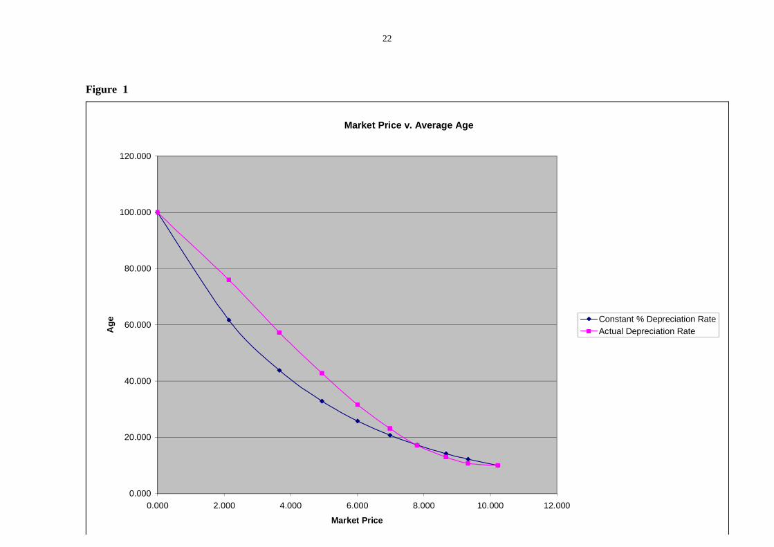
illustrate how uncertainty impacts on depreciation, table 4 shows how value, expected

economic life and second hand price vary with the current level of operating cost.

Clearly, as current operating cost rises toward the level at which replacement is

activated, average life falls to zero, as does the second hand value. Although the

determinant of second value is the current level of operating cost, it is of some interest

to consider the implied relationship between the second hand value and the average

life expectancy. Interestingly, the rate of depreciation under uncertainty, for the

benchmark values, shows a more linear rate of depreciation than would occur if

depreciation was exponential (a constant rate depreciation curve is included - in

column 4 of table 4 - for comparison purposes).

16

5. CONCLUDING COM M ENTS

It was probably George Terborgh [1949] who first advanced the assumption, when

examining the replacement investment decision, that operating expenses tend to

increase at a constant rate over time. This paper extends this type of analysis to the

case where the evolution of operating cost is uncertain. The impact of uncertainty has

been treated before in the literature, but generally in different ways (usually in a

discrete time framework, and usually featuring components which have a risk of

catastrophic failure) and there has been relatively little (if any) study of comparative

statics properties of such models. This paper extends Terborgh’s ‘exponential model’

to the uncertainty case, and then conducts a systematic study of both qualitative and

quantitative properties of the model.

The aim in undertaking this analysis was to provide a model which is relatively easy

to work with numerically (the basic equation which determines the replacement

decision can be readily solved using standard spreadsheet functions (such as

SOLVER in EXCEL). Furthermore, it was shown that the proxy for average

economic life (equation (25)) was usually a fairly good approximation,9 and again, this

was readily computable using a simple spreadsheet. For applications where the

underlying assumptions are reasonably plausible, it could be used as a basis for

assessing the timing of replacement investment. Naturally, there are many other

considerations outwith those considered here which might affect such decisions; in

such circumstances it may be possible to use the model to put an opportunity cost on

9 Table 2 indicates that the proxy only starts to seriously underestimate average economic life when there is high volatility and/or very low rates of increase in operating cost.

17

those considerations. For example, consider a fleet of company cars (or a bus

company); it is possible to assess not only the trigger points at which replacement

should be undertaken, but it is also possible to estimate the costs of varying from

these choices. For example, if the company does not wish to see its sales force in cars

older than a certain age, it is possible, using this model, to quantify the cost of

shortening the age at which such company cars are replaced.

Apart from the intrinsic importance of the decision itself, replacement investment is

of course important from a macro-economic perspective, in that if might cast some

light of the relationship between interest rates and levels of investment (how steep the

marginal efficiency of capital schedule is). In thinking about such issues, it is useful

to recognise the importance of uncertainty. In the above model, an increase in the

steady state rate of interest not only affects costs directly; it also has an effect in that

firms will choose to extend the economic life of the plant and equipment they operate;

at the benchmark values for example, the elasticity of (average) economic life to

changes in the rate of interest was in the region of 0.1 under certainty, and in the same

ball park under uncertainty. This is not only fairly inelastic, but is also a fairly

typically value, given plausible values for volatility and the other parameters

involved. Thus, the model is also suggestive that changes in the rate of interest do not

have great impacts on replacement timing. Such observations are supportive of the

case that, if there is a relationship at all, the marginal efficiency of capital schedule

may be fairly steep (and hence so too the IS curve, in an ISLM framework).10

10 An increase in interest rates naturally raises financing costs and so there could be longer run output consequences which would also need to be considered; the above discussion presumes the ‘quantity’ of plant in service at a point in time is unaffected by the change in the level of interest. In such

18

REFERENCES Dixit A.K., 1989, Entry and exit decisions under uncertainty, Journal of Political Economy, 97, 620-638. Dixit A.K., 1993, The art of smooth pasting, Harwood Academic publishers, Chur, Switzerland. Dixit A. and Pindyck R., 1994, Investment under uncertainty, Princeton University press, Princeton, New Jersey. Dumas B., 1991, Super contact and related optimality conditions, Journal of Economic Dynamics and Control, 15, 675-685. Genesove D, 1993, Adverse selection in the wholesale used car market, Journal of Political Economy, 101, 644-665. Hotelling H., 1925, A general mathematical theory of depreciation, Journal of the American Statistical Society, 20, 340-353. Kim J-C, 1985, The market for “Lemons” reconsidered: A model of the used car market with asymmetric information, American Economic Review, 75, 836-843. McDonald R. and Siegel D., 1986, The value of waiting to invest, Quarterly Journal of Economics, 101, 707-728. Merrett A.J. and Sykes A., 1965, The finance and analysis of capital projects, Longmans, London. Pierskalla W.P. and Voelker J.A., 1976, A survey of maintenance models: the control and surveillance of deteriorating systems, Naval Research Logistics Quarterly, 23, 353-388. Pindyck R.S., 1988, Irreversible investment, capacity choice and the value of the firm, American Economic Review, 78, 969-985. Rust J., 1985, Stationary equilibrium in a market for durable assets, Econometrica, 53, 783-805. Rust J., 1987, Optimal replacement of GMC bus engines: an empirical model of Harold Zurcher, Econometrica, 55, 999-1033. Sherif Y.S. and Smith M.L., 1981, Optimal maintenance models for systems subject to failure – A review, Naval Research Logistics Quarterly, 32, 47-74.

circumstances, a rise in interest rates tends to raise economic life (albeit only slightly); in a steady state, that would mean less per period investment in new equipment.

19

Smith V., 1961, Investment and Production, Harvard University Press, Cambridge M.A. Terborgh G., 1949, Dynamic Equipment Policy, McGraw-Hill, New York.

20

Table 2: Economic Life as a function of various parameters

Parameter Value c certT T̂ T Ts

Bench 35.870 8.197 8.515 10.09 0.048

Panel (a) Mark

θ 0.05 29.888 18.326 21.897 37.445 0.411 0.1 31.382 10.979 11.437 14.723 0.096 0.15 35.870 8.197 8.515 10.09 0.048 0.25 42.344 5.688 5.773 6.383 0.022 0.5 56.713 3.457 3.471 3.665 0.008 1 80.639 2.085 2.087 2.149 0.003

Panel (b) σ 0.000001 34.198 8.197 8.197 8.197 0.000

0.01 34.202 8.197 8.198 8.199 0.002 0.1 34.606 8.197 8.276 8.649 0.020 0.2 35.870 8.197 8.515 10.100 0.049 0.5 45.781 8.197 10.142 55.753 1.000

Panel (c ) θ 0.165 36.860 7.656 7.906 9.168 0.041r 0.11 36.454 8.280 8.623 10.112 0.049K 110 37.782 8.533 8.862 10.417 0.050S 11 35.676 8.162 8.479 10.054 0.049

0c 11 37.695 7.902 8.211 9.685 0.047σ 0.22 36.234 8.197 8.583 10.479 0.057

Benchmark Parameter values: 00.1, 0.15, 100, 10, 10, 0.2r K S cθ σ= = = = = =

Table 3: Elasticities at benchmark values

Parameter c certT T̂ T #

θ 0.28 -0.66 -0.72 -0.91 r 0.16 0.10 0.13 0.02 K 0.53 0.41 0.41 0.32 S -0.05 -0.04 -0.04 -0.04

0c 0.51 -0.36 -0.36 -0.40 σ 0.10 0.00 0.08 0.39

# The elasticities calculated here are subject only to machine error in numerical computations of

solutions – except for those for T . Given that T is estimated by simulation and manifests a standard error of around 0.05, the estimates of elasticity in the final column are significantly less robust.

21

Table 4: Example of Depreciation under Uncertainty

0c T Average age Second hand Price if constant (exponential) depreciation

Theoretical second hand price

( )p c

10.000 10.230 0.000 100.000 100.000 12.875 8.084 2.146 61.687 75.928 15.749 6.567 3.664 43.842 57.278 18.623 5.289 4.941 32.886 42.776 21.498 4.215 6.015 25.827 31.602 24.372 3.242 6.988 20.745 23.180 27.247 2.428 7.802 17.271 17.095 30.121 1.557 8.673 14.198 13.027 32.996 0.896 9.334 12.235 10.728 35.870 0.000 10.230 10.000 10.000

22

Figure 1

Market Price v. Average Age

0.000

20.000

40.000

60.000

80.000

100.000

120.000

0.000 2.000 4.000 6.000 8.000 10.000 12.000

Market Price

Ag

e Constant % Depreciation RateActual Depreciation Rate

23

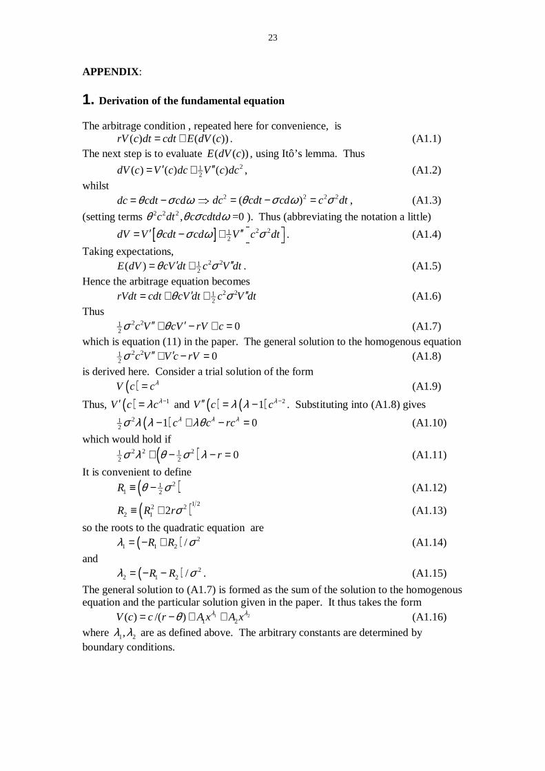
APPENDIX:

1. Derivation of the fundamental equation

The arbitrage condition , repeated here for convenience, is ( ) ( ( ))rV c dt cdt E dV c= + . (A1.1)

The next step is to evaluate ( ( ))E dV c , using Itô’s lemma. Thus

212( ) ( ) ( )dV c V c dc V c dc′ ′′= + , (A1.2)

whilst dc cdt cdθ σ ϖ= − � 2 2 2 2( )dc cdt cd c dtθ σ ϖ σ= − = , (A1.3)

(setting terms 2 2 2,c dt c cdtdθ θ σ ϖ =0 ). Thus (abbreviating the notation a little)

[ ] 2 212dV V cdt cd V c dtθ σ ϖ σ′ ′′

� �= − + � � . (A1.4)

Taking expectations, 2 21

2( )E dV cV dt c V dtθ σ′ ′′= + . (A1.5) Hence the arbitrage equation becomes

2 212rVdt cdt cV dt c V dtθ σ′ ′′= + + (A1.6)

Thus 2 21

2 0c V cV rV cσ θ′′ ′+ − + = (A1.7) which is equation (11) in the paper. The general solution to the homogenous equation

2 212 0c V V c rVσ ′′ ′+ − = (A1.8)

is derived here. Consider a trial solution of the form ( )V c cλ= (A1.9)

Thus, ( ) 1V c cλλ −′ = and ( ) ( ) 21V c cλλ λ −′′ = − . Substituting into (A1.8) gives

( )212 1 0c c rcλ λ λσ λ λ λθ− + − = (A1.10)

which would hold if

( )2 2 21 12 2 0rσ λ θ σ λ+ − − = (A1.11)

It is convenient to define

( )211 2R θ σ≡ − (A1.12)

( )1 22 22 1 2R R rσ≡ + (A1.13)

so the roots to the quadratic equation are

( ) 21 1 2 /R Rλ σ= − + (A1.14)

and ( ) 2

2 1 2 /R Rλ σ= − − . (A1.15)

The general solution to (A1.7) is formed as the sum of the solution to the homogenous equation and the particular solution given in the paper. It thus takes the form 1 2

1 2( ) /( )V c c r A x A xλ λθ= − + + (A1.16)

where 1 2,λ λ are as defined above. The arbitrary constants are determined by boundary conditions.

24

2. Comparative Statics Analysis

There are two equations determining c and 1λ ; the latter is the positive root of the

fundamental equation (A11). Defining 2v σ≡ and the function

( )21 12 2( )f v v rλ λ θ λ≡ + − − (A2.1)

then 1λ satisfies 1( ) 0f λ = (A2.2)

Note that 1λ is defined as the positive root of the equation (A2.2), such that

( ) ( )1 1/ 222 1

1 2

12

vv vr

v v

θλ θ

− � �= − + − +� � . (A2.3)

Note also that 1λ is strictly increasing in r. If we set r θ= , then (A2.3) simplifies to give

( )

( ) ( ) ( ) ( )

11/ 22 2 21

1 4

1 1 11/ 222 2 212

12

11

vv v v

v vv v v

vv v v v

θλ θ θ θ

θ θ θθ

− � �= − + − + +� �

− − +� �= − + + = − + =� �

(A2.4)

It thus follows that, since 1 / 0rλ∂ ∂ > , that

1 1rθ λ> <�< > (A2.5)

The other condition established in the paper is that, defining the function

( ) [ ]10 0( , ) 1 ( )( )g c c c c c K S rλ λλ λ θ λ−= − − + + − − (A2.6)

that

1( , ) 0g c λ = (A2.7)

Denote a generic parameter as ψ (i.e. 0, , , , ,r S K c vψ θ= ). Then

1 1 1 1 1 1( ) ( ) ( ) ( )0

f d f d f f

d d

λ λ λ λ λ λψ λλ ψ ψ ψ

∂ ∂ ∂ ∂+ = = −∂ ∂∂ ∂

(A2.8)

and

1 1 1 1( , ) ( , ) ( )0

g c d g c dc g

d c d

λ λ λ λλ ψ ψ ψ

∂ ∂ ∂+ + =∂ ∂ ∂

(A2.9)

so the comparative statics derivative is given as

1 1 1 1( , ) ( ) ( , )dc g c d g g cd cd

λ λ λ λλ ψ ψψ

�∂ ∂ ∂= − +

� ∂ ∂ ∂

� � (A2.10)

which, using (A2.8), means that

1 1 1 1 1( ) ( , ) ( ) ( ) ( , )dc g g c f f g c

cd

λ λ λ λ λψ λ ψ λψ

� �� �∂ ∂ ∂ ∂ ∂= − − ×

� �� �∂ ∂ ∂ ∂ ∂

� �� � (A2.11)

To begin, we need to establish the various partial derivatives (evaluating these at

1,c λ , as follows: from (A2.1),

1( ) / 0f Kλ∂ ∂ = , (A2.12)

1( ) / 0f Sλ∂ ∂ = , (A2.13)

1 0( ) / 0f cλ∂ ∂ = , (A2.14)

1( ) / 1f rλ∂ ∂ = − <0 (A2.15)

25

1 1( ) /f λ θ λ∂ ∂ = >0 (A2.16)

( )11 1 12( ) / 1f vλ λ λ∂ ∂ = − (A2.17)

whilst from (A2.6)

1 1( , ) / ( )g c K rλ θ λ∂ ∂ = − <0 (A2.18)

1 1( , ) / ( )g c S rλ θ λ∂ ∂ = − − >0 (A2.19)

( )( )11 111 1

1 0 1 0 1 1 0( , ) / 1 /g c c c c c cλλ λλ λ λ λ −− −∂ ∂ = − + = − (A2.20)

1 1( , ) / ( )g c r K Sλ λ∂ ∂ = − >0 (A2.21)

1 1( , ) / ( )g c K Sλ θ λ∂ ∂ = − − <0 (A2.22)

1( , ) / 0g c vλ∂ ∂ = (A2.23) Finally, note that from (A2.1),

( )11 1 2( ) /f v vλ λ λ θ∂ ∂ = + − . (A2.24)

From (A2.3) (in which the positive square root is taken), clearly this is positive. From (A2.6),

( ) ( ) ( ) ( )( )11 11 1 1 0 1 0( , ) / 1 1 1 1 /g c c c c c c

λλ λλ λ λ λ−∂ ∂ = − − − = − − . (A2.25)

Given this is the denominator in (A2.11), its sign is crucial for comparative statics

results. Since 0 /c c <1 and 1 0λ > , clearly ( ) 1

01 /c cλ− >0, and so from (A2.5),

1 11 ( , ) / 0r g c cθ λ λ> < >� � ∂ ∂< > < (A2.26)

The term /g λ∂ ∂ is a little more tricky. From (A2.6),

( ) [ ]10 0( , ) / ( )( )g c c c c c K S rλ λ

λλ λ θ−∂∂∂ ∂ = − − + + − − (A2.27)

Now,

( ) ( ) ( )1 1 10 0 0c c c c c cλ λ λλ λ λ

λ λ λ− − −∂ ∂ ∂

∂ ∂ ∂= + (A2.28)

and

( )1 1 lnc c cλ λλ

− −∂∂ = − (A2.29)

( )0 0 0lnc c cλ λλ∂

∂ = (A2.30)

so

( ) ( ) [ ][ ]

1 10 0 0

1 10 0 0 0

/ ( )( )

ln ln ( )( )

g c c c c c c K S r

c c c c c c c c K S r

λ λλ λλ λ

λ λλ λ

λ θθ

− −∂ ∂∂ ∂

− −

∂ ∂ = − − − + + − −= − + − + + − −

(A2.31)

so evaluating at 1,c λ and simplifying a little gives

( ) ( ) [ ]1

1 0 0 0( , ) / / ln / 1 ( )( )g c c c c c c c K S rλλ λ θ

� �∂ ∂ = − + + − −� � . (A2.32)

Now (A2.6) and (A2.7) imply that :

( ) [ ]1 111 1 0 0 1( , ) 1 ( )( ) 0g c c c c c K S rλ λλ λ θ λ−= − − + + − − = (A2.33)

and so

( ) 1 111 0

01

1( )( )

c c cc K S r

λ λλθ

λ

−� �

− −� �

+ − − = − . (A2.34)

Using this to replace the term [ ]0 ( )( )c K S r θ+ − − in (A2.32) gives

26

( ) ( )( ) 1 1

1

11 0

1 0 01

1( , ) / / ln / 1

c c cg c c c c c c

λ λλ λ

λ λλ

−� �� �

− −� �� � � �∂ ∂ = − −� � � �

� � (A2.35)

�

( ) ( )( )

( ) ( ) ( )( )

1

1

1 1

0

1 0 01

1 0 0 0 11

1 /( , ) / / ln / 1 1

/ ln / 1 1 /

c cg c c c c c c c

cc c c c c c

λλ

λ λ

λ λλ

λ λλ

� �� �− � �� �

∂ ∂ = − − − � �� �

� � � �= − − − +

�

( ) ( ) ( )( )1 1

1 1 0 0 01

( , ) / / ln / 1 /c

g c c c c c c cλ λλ λ λ

λ

� �∂ ∂ = − −� �

�

( ) ( )( )1 1

1 0 01

( , ) / / 1 ln / 1c

g c c c c cλ λλ λ

λ

� �∂ ∂ = − −� � (A2.36)

Write ( ) 1

0 /z c cλ≡ , so that, with 00 / 1c c< < and 1 0λ > , clearly 0 1z< < . The sign

of above expression then depends on the term [ ]( ) 1 ln 1W z z z≡ − − (A2.37)

First note that [ ] [ ]( ) / 1 ln 1/ ln 0dW z dz z z z z= − + − = − > (since (0,1)z ∈ ) so ( )W z

is strictly increasing on (0,1). Also note that (1) 0W = , hence it follows, for all z such

that 0 1z< < , that ( ) 0W z < . Given 1/ 0c λ > this implies

1( , ) / 0g c λ λ∂ ∂ < (A2.38) This completes the preliminaries necessary for determining the comparative statics results, which can now be computed using (A2.11). Capital cost: Here, / 0f K∂ ∂ = , and / ( )g K r θ λ∂ ∂ = − so (A2.11) becomes

( )( )( )( )1

1

/ / / / / /( ) / 0 / /

( ) /

dc dK g K g f K f g cr g f g cr g c

λ λθ λ λ λ

θ λ

= − ∂ ∂ − ∂ ∂ ×∂ ∂ ∂ ∂ ∂ ∂= − − − ∂ ∂ × ∂ ∂ ∂ ∂= − ∂ ∂

Now, 1 0λ > and 0r rθ θ> >� −< < and (for all , 0,r rθ θ> ≠ ) from (A2.26)

1( , ) / 0r g c cθ λ> >� ∂ ∂< < hence, it follows that

(for all , 0,r rθ θ> ≠ ), / 0dc dK > (A2.39)

27

Salvage Value: The analysis parallels that for capital cost. Here / 0f S∂ ∂ = , and 1/ ( )g S r θ λ∂ ∂ = − −

so 1/ ( ) /dc dS r g cθ λ= − − ∂ ∂ . Thus (for all , 0,r rθ θ> ≠ ), / 0dc dS < (A2.40)

Initial Operating Cost:

Here 0/ 0f c∂ ∂ = , and ( )( )1 1

0 1 0/ 1 /g c c cλλ −∂ ∂ = − so

( )( )( )( ) ( )( )

( )( )1

1

0 0 01

1 0

1

1 0

/ / / / / /

1 / / 0 / /

1 / /

dc dc g c g f c f g c

c c g f g c

c c g c

λ

λ

λ λλ λ λ

λ

−

−

= − ∂ ∂ − ∂ ∂ × ∂ ∂ ∂ ∂ ∂ ∂

= − − − ∂ ∂ × ∂ ∂ ∂ ∂

= − − ∂ ∂

Now, 1 0λ > and 00 / 1c c< < and (for all , 0,r rθ θ> ≠ ) from (A2.26)

1( , ) / 0r g c cθ λ> >� ∂ ∂< < . Also, ( ) ( )1 11 1

1 0 01 / 1 1 / 0r c c c cλ λθ λ − −> < > <� � � −< > < > .

It thus follows that (for all , 0,r rθ θ> ≠ ), 0/ 0dc dc > (A2.41)

Volatility: Here

( )( )/ / / / / /dc dv g v g f v f g cλ λ= − ∂ ∂ − ∂ ∂ × ∂ ∂ ∂ ∂ ∂ ∂

where , / 0g v∂ ∂ = , / 0g λ∂ ∂ < , and / 0f λ∂ ∂ > so

( ) ( )/ / /Sign dc dv Sign f v g c= − ∂ ∂ ∂ ∂

Now, ( )11 12/ 1f v λ λ∂ ∂ = − and from (A2.5), 1 1rθ λ> <�

< > , so

1 1 / 0r f vθ λ> < <� � ∂ ∂< > > .

However, 1( , ) / 0r g c cθ λ> >� ∂ ∂< < from (A2.26). Hence

(for all , 0,r rθ θ> ≠ ), / 0dc dσ > (A2.42) Interest rate: Here,

( )( )/ / / / / /dc dr g r g f r f g cλ λ= − ∂ ∂ − ∂ ∂ ×∂ ∂ ∂ ∂ ∂ ∂

where / 1f r∂ ∂ = − <0, 1/ ( )g r K S λ∂ ∂ = − >0, 1( , ) / 0g c λ λ∂ ∂ < and

( )11 2/f v vλ λ θ∂ ∂ = + − >0.

Hence, /dc dr is of ambiguous sign. Operating cost trend: Here

( )( )/ / / / / /dc d g g f f g cθ θ λ θ λ= − ∂ ∂ − ∂ ∂ ×∂ ∂ ∂ ∂ ∂ ∂

where 1/f θ λ∂ ∂ = >0, 1/ ( ) 0g K Sθ λ∂ ∂ = − − < , / 0g λ∂ ∂ < , and / 0f λ∂ ∂ > . Hence, /dc dθ is of ambiguous sign.