optimal housing, consumption, and investment decisions...

Introduction Model Full flexibility Comparative statics Limited flexibility

Optimal Housing, Consumption, and

Investment Decisions over the Life-Cycle

Holger Kraft1 Claus Munk2

1Goethe University Frankfurt, Germany

2Aarhus University, Denmark

Management Science, vol. 57(6), pp. 1025–1041, 2011

AARHUS UNIVERSITY AU


Outline

1 Introduction

2 Model

3 Full flexibility

4 Comparative statics

5 Limited flexibility


Overview and motivation

Important features in life-cycle decisions of individuals:

interest rate risk(Sørensen JFQA99; Campbell/Viceira AER01; Munk/Sørensen JBF04)

risky labor income(Bodie/Merton/Samuelson JEDC92; Cocco/Gomes/Maenhout RFS05; Munk/Sørensen

JFE-forthcoming)

housing decisions(Cocco RFS05; Yao/Zhang RFS05; Van Hemert wp08)

Existing papers with income and housing:

coarse and computationally intensive numerical solutiontechniques with unknown precisionprovide limited understanding of economic forces at play

This paper : explicit, “Excel-ready” solutions


Financial assets

Available assets: cash, bond(s), stock

Short-term interest rate (= return on cash ):

drt = κ (r − rt ) dt − σr dWrt

Price Bt = B(rt , t) of an arbitrary bond :

dBt = Bt [(rt + λBσB(rt , t)) dt + σB(rt , t) dWrt ]

Zero-coupon bond: But = exp{−a(u − t)− Bκ(u − t)rt}, where

Bκ(τ) = 1κ (1− e−κτ ).

Stock price:

dSt = St

[(rt + λSσS) dt + σS

(ρSB dWrt +

√1− ρ2

SB dWSt

)]


Housing

“Unit” house price Ht :

dHt

Ht=(

rt + λHσH − r imp)

dt + σH (ρHB dWrt + ρHS dWSt + ρH dWHt )

Housing positions:

owning ϕot housing units

renting ϕrt units at continuous rental rate per unit is νHt

investing in REITs , ϕRt units, with total return dHtHt

+ ν dt

Housing consumption: ϕCt = ϕot + ϕrt

Housing investment: ϕIt = ϕot + ϕRt


Labor incomeIncome rate Yt until retirement at T :

dYt

Yt= (µY (t) + brt ) dt + σY (t) (ρYB dWrt + ρYS dWSt + ρY dWHt )

In retirement: Yt = ΥYT , t ∈ (T ,T ].

Human wealth/capital:The human capital is

Lt ≡ EQt

[∫ T

te−

∫ st ru duYs ds

]=

YtF (t , rt ), t < T ,

YT F (t , rt ), t ∈ [T ,T ],

where

F (t , r) =

∫ T

t e−A(t,s)−(1−b)Bκ(s−t)r ds + Υ∫ T

T e−A(t,s)−(Bκ(s−t)−bBκ(T−t))r ds, t < T ,

Υ∫ T

t e−a(s−t)−Bκ(s−t)r ds, t ≥ T

Here A(t , s) and A(t ,S) are deterministic functions stated in Appendix A.


Wealth

Financial/tangible wealth: Xt

Total wealth: Xt + Lt

dXt = πStXtdSt

St+ πBtXt

dBt

Bt+ [Xt (1− πSt − πBt )− (ϕot + ϕRt )Ht ] rt dt

+ ϕot dHt + ϕRt (dHt + νHt dt)− ϕrtνHt dt − ct dt + Yt dt

= [Xt (rt + πStλSσS + πBtλBσBt ) + ϕItλ′HσHHt − ϕCtνHt − ct + Yt ] dt

+ (πStXtρSBσS + πBtXtσBt + ϕItHtρHBσH) dWrt

+

(πStXtσS

√1− ρ2

SB + ϕItHt ρHSσH

)dWSt + ϕItHt ρHσH dWHt ,

whereϕCt ≡ ϕot + ϕrt , ϕIt ≡ ϕot + ϕRt .


The individual’s utility maximization problem

J(t , x , r ,h, y) = sup(c,ϕC ,ϕI ,πB ,πS)∈At

Et

[ ∫ T

te−δ(u−t) 1

1− γ

(cβu ϕ

1−βCu

)1−γds

+ εe−δ(T−t) 11− γ

X 1−γT

]


Parameter values used in illustrations

Preferences and wealth: X0 = USD 20,000; δ = 0.03; γ = 4;β = 0.8; ε = 0; T = 30; T = 50

Interest rate and bond: κ = 0.2; r0 = r = 0.02; σr = 0.015;λB = 0.1; Tbond = 20 (running); σB = 0.0736

Stock: σS = 0.2, λS = 0.25, ρSB = 0

Housing: σH = 0.12; λH = 0.325; r imp = ν = 0.05 (soµH = 0.9%); ρHB = 0.65; ρHS = 0.5; H0 = USD 250 per “averagestandard” sq. footREITS drift 0.9%+5%=5.9%, low vol attractive investment

Labor income: Y0 = USD 20,000; b = 0.5; µY (t) = 0.01;σY (t) = 0.075; ρYB = −0.3; ρYS = 0; ρHY = 0.3509 (ensuresspanning)


Solution to the HJB-equation...

J(t , x , r , h, y) =1

1− γ g(t , r , h)γ(x + yF (t , r))1−γ ,

g(t , r , h) = ε1γ e−Dγ (T−t)− γ−1

γBκ(T−t)r +

ην

1− β hk∫ T

te−d1(u−t)−β γ−1

γBκ(u−t)r du.

Here k = (1− β)(1− 1/γ), η = β1/γ(βν

1−β

)k−1, and Dγ(τ) and d1(τ) are

stated in the appendix.

πS ≡πSx

x + yF=

1γ

ξS

σS− σY (t)ζS

σS

yFx + yF

,

πB ≡πBx

x + yF=

1γ

ξB

σB−(σY (t)ζB

σB

yFx + yF

− σr

σB

yFx + yF

Fr

F

)− σr

σB

gr

g,

πI ≡hϕI

x + yF=

1γ

ξI

σH− σY (t)ζI

σH

yFx + yF

+hgh

g

c = ηβν

1− β hk x + yFg

, ϕC = ηhk−1 x + yFg

.

(when t ∈ [T ,T ]: σY (t) = 0 and y is to be replaced by YT )


Expected consumption over the life-cycle

ct = ηβν

1− βHkt

Xt + YtF (t , rt )

g(t , rt ,Ht )νHt ϕCt =

1− ββ

ct

0

100

200

300

400

500

600

700

800

900

0

10

20

30

40

50

60

0 10 20 30 40 50

Exp

ect

ed

ho

usi

ng

un

its

Exp

ect

ed

co

nsu

mp

tio

n (

in t

ho

usa

nd

s)

Time, years

Perishable

House expend

House units


Optimal investments – fractions of total wealth

Stocks πS =1γ

ξS

σS−σY ζS

σS

yFx + yF

,

5.5% 0↔ 31%

Bonds πB =1γ

ξB

σB−(σY ζB

σB− σr

σB

Fr

F

)yF

x + yF− σr

σB

gr

g,

−57% 0↔ 141% 0↔ −43% 49%

House πI =1γ

ξI

σH−σY ζI

σH

yFx + yF

+hgh

g86% 0↔ −104% 15%

speculative adjust for human wealth hedge


Optimal investments and the composition of wealth

-60%

-40%

-20%

0%

20%

40%

60%

80%

100%

120%

0.0 0.2 0.4 0.6 0.8 1.0

Inve

stm

en

t /

Tota

l we

alth

Human wealth / Total wealth

Bond

Stock

House

Bond (retired)

Stock (retired)

House (retired)

Assuming fixed r , h and fixed FrF ,

grg (vary little over life anyway)

Main life-cycle effect is change in ratio of human-to-total wealth


Expected wealth over the life-cycle

0

100

200

300

400

500

600

700

800

0 10 20 30 40 50

Exp

ect

ed

we

alth

(in

th

ou

san

ds)

Time, years

Total wealth

Financial wealth

Human wealth


Expected investments over the life-cycle

-400

-200

0

200

400

600

800

0 10 20 30 40 50

Exp

ect

ed

inve

stm

en

t (i

n t

ho

usa

nd

s)

Time, years

Bond

Stock

House


Housing consumption and over the life-cycle

0

200

400

600

800

1000

1200

1400

1600

1800

2000

2200

2400

0 10 20 30 40 50

Exp

ect

ed

ho

usi

ng

un

its

Time, years

Housing cons

Housing inv

Housing hedge


Robustness of results

effects of γ, ε, H0, σH , Y0, σY , Υ, ρHY : see paper and appendix

here: effects of empirically estimated life-cycle income profiles,cf. Cocco, Gomes & Maenhout (RFS 2005)


Expected income over the life-cycle for three

educational groups

0

5

10

15

20

25

30

35

40

45

50

25 35 45 55 65 75 85

Exp

ect

ed

an

nu

al in

com

e (

tho

usa

nd

s)

Age, in years

no high

high

college

constant


Expected wealth over the life-cycle for three

educational groups

0

200

400

600

800

1000

1200

25 35 45 55 65 75 85

Exp

ect

ed

we

alth

(th

ou

san

ds)

Age, in years

Human, no high

Total, no high

Financial, no high

Human, high

Total, high

Financial, high

Human, college

Total, college

Financial,college


Expected investments over the life-cycle for three

educational groups

-600

-400

-200

0

200

400

600

800

1000

1200

25 35 45 55 65 75 85

Exp

ect

ed

inve

stm

en

t (i

n t

ho

usa

nd

s)

Age, in years

Stock, no high

House, no high

Bond, no high

Stock, high

House, high

Bond, high

Stock, college

House, college

Bond, college


Consumption of and investment in housing over the

life-cycle for three educational groups

-500

0

500

1000

1500

2000

2500

3000

3500

25 35 45 55 65 75 85

Exp

ect

ed

ho

usi

ng

un

its

Age, in years

Cons, no high

Inv, no high

Cons, high

Inv, high

Cons, college

Inv, college


Limited flexibility in housing decisions

Scenarios considered:

1 constant number of units of housing consumed (closed-formsolution)

2 infrequent adjustments of housing investment and housingconsumption (MC results)

Percentage wealth-equivalent utility loss L due to limited flexibility:

J (t , x [1− L], r ,h, y [1− L]) = Jlimited(t , x , r ,h, y)


Utility loss of constant housing consumption

8%

10%

12%

14%

16%

18%

20%

We

alt

h lo

ss c

om

pa

red

to

fu

ll f

lex

ibil

ity

0%

2%

4%

6%

0 100 200 300 400 500 600 700 800 900 1000

We

alt

h lo

ss c

om

pa

red

to

fu

ll f

lex

ibil

ity

Fixed level of housing units

Note: minimum loss is 0.26% for a constant housing consumption (USD 1,550 out of total wealth USD 596,400).

The individual can almost completely compensate for inflexibility in housing consumption by adjusting perishable consumption and

investments


Loss due to infrequent housing adjustmentsSimulate BM’s and thus wealth, income (10,000 paths, 250 steps/year)When adjusted, use policies optimal with continuous adjustments

Initial income 10, 000 Initial income 20, 000

Adjustment frequency 2 years 5 years 2 years 5 years

Infrequent ϕC , frequent ϕI 0.03% 0.08% 0.03% 0.08%

Infrequent ϕI , frequent ϕC 0.21% 1.35% 0.23% 1.43%

Infrequent ϕC and ϕI 0.24% 1.52% 0.26% 1.61%

suggests moderate welfare effects of a well-functioning market forREITs or CSI housing contracts

suggests moderate effects of housing transactions costs

Introduction General market setting Mean reversion in stock prices Stochastic interest rates Conclusion

Portfolio and Consumption Choice withStochastic Investment Opportunities and

Habit Formation in Preferences(Journal of Economic Dynamics and Control, 2008)

Claus Munk

August 2012

AARHUS UNIVERSITY AU


Outline

1 Introduction

2 General market setting

3 Mean reversion in stock prices

4 Stochastic interest rates

5 Conclusion


Motivation

Investment opportunities vary stochastically over timeI Many papers on optimal portfolio and consumption choice with

stochastic investment opportunitiesI Almost all assume utility of terminal wealth, E[u(WT )], or

time-separable utility of consumption, U(c) = E[∫ T

0 e−δtu(ct ) dt].

Many economists argue that individuals develop habits forconsumption.Preferences with habit formation help explain asset pricingpuzzles (Sundaresan 1989, Constantinides 1990, Campbell andCochrane 1999).Earlier studies of individuals’ optimal portfolio and consumptionchoice under habit formation assume constant investmentopportunities.


Objectives

Derive optimal portfolio and consumption choice for individualswith habit formation in markets with stochastic investmentopportunities.Consider both general dynamics of investment opportunities andconcrete, special cases.Do stochastic investment opportunities affect the decisions ofindividuals with habit formation differently than individuals withtime-additive preferences?Are the effects of habit formation in preferences on optimaldecisions different in markets with stochastic investmentopportunities than in markets with constant investmentopportunities?


Literature review

time-additive utility habit formation utilityconstant Samuelson (1969) Sundaresan (1989)inv.opp. Merton (1969, 1971) Constantinides (1990)

Ingersoll (1992)

general Merton (1971, 1973) Detemple and Zapatero (1992)stochastic Karatzas-Lehoczky-Shreve (1987) Detemple and Karatzas (2003)inv.opp. Cox and Huang (1989, 1991) Schroder and Skiadas (2002)

Liu (2007) THIS PAPERMunk and Sørensen (2004)

concrete Sørensen (1999) THIS PAPERstochastic Brennan and Xia (2000)inv.opp. Kim and Omberg (1996)

Wachter (2002)


The financial market

Basic uncertainty modeled by n-dimensional SBM z = (zt )

“Bank account”: rate of return rt

n risky assets: dPt = diag(Pt ) [(rt1 + σtλt ) dt + σt dzt ]

Assume σt non-singularComplete market – unique state-price deflator:

ξt = exp

{−∫ t

0rs ds −

∫ t

0λ>

s dzs −12

∫ t

0‖λs‖2 ds

}

(and unique risk-neutral probability measure)


The individual...

... wants to maximize

U(c) = E

[∫ T

0e−δt 1

1− γ(ct − ht )

1−γ dt

],

where

ht = h0e−βt + α

∫ t

0e−β(t−s)cs ds.

Note: requires ct ≥ ht for all t [not necessarily very restrictive].... chooses a consumption strategy c = (ct ) and a portfoliostrategy π = (πt ) under budget constraint Et

[∫ Ttξsξt

cs ds]≤Wt .

... receives no labor income.Wealth dynamics: dWt = [Wt (rt + π>

t σtλt )− ct ] dt + Wtπ>t σt dzt .

Indirect utility:Jt = sup(c,π)∈A(t) Et

[∫ Tt e−δ(s−t) 1

1−γ (cs − hs)1−γ ds].


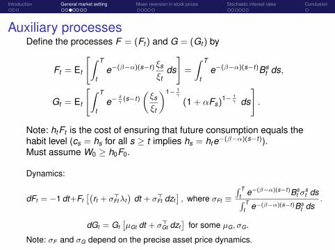
Auxiliary processesDefine the processes F = (Ft ) and G = (Gt ) by

Ft = Et

[∫ T

te−(β−α)(s−t) ξs

ξtds

]=

∫ T

te−(β−α)(s−t)Bs

t ds,

Gt = Et

[∫ T

te−

δγ (s−t)

(ξs

ξt

)1− 1γ

(1 + αFs)1− 1γ ds

].

Note: htFt is the cost of ensuring that future consumption equals thehabit level (cs = hs for all s ≥ t implies hs = hte−(β−α)(s−t)).Must assume W0 ≥ h0F0.

Dynamics:

dFt = −1 dt+Ft[(

rt + σ>Ftλt

)dt + σ>

Ft dzt], where σFt ≡

∫ Tt e−(β−α)(s−t)Bs

t σst ds∫ T

t e−(β−α)(s−t)Bst ds

.

dGt = Gt[µGt dt + σ>

Gt dzt]

for some µG, σG.

Note: σF and σG depend on the precise asset price dynamics.


Theorem 1

Under two regularity conditions, the solution is as follows.Optimal consumption: c∗t = h∗t + (1 + αFt )

− 1γ

W∗t −h∗

t FtGt

.

Indirect utility: Jt = 11−γGγ

t (W ∗t − h∗t Ft )

1−γ.

Optimal portfolio:

π∗t =W ∗

t − h∗t Ft

W ∗t

1γ

(σ>t )−1λt︸︷︷︸

speculative

+W ∗

t − h∗t Ft

W ∗t

(σ>t )−1σGt︸︷︷︸

hedge

+h∗t Ft

W ∗t

(σ>t )−1σFt︸︷︷︸

habit “insurance”

.

Note: Both the speculative term and the hedge term are dampeneddue to habit formation. Additional effect on hedge term via G andhence σG.Jointly allowing for habit and stochastic IO’s has effects beyond theirseparate effects! Quantitatively important?


Markovian asset pricesAssume rt = r(xt ) and λt = λ(xt ), where

dxt = m(xt ) dt + v(xt ) dzt .

Then Bst = Bs(xt , t), where Bs(x , t) solves

12

tr(∂2Bs

∂x2 v(x)v(x)>)

+ (m(x)− v(x)λ(x))>∂Bs

∂x+∂Bs

∂t− r(x)Bs = 0

with Bs(x , s) = 1, and σFt becomes

σFt =

∫ Tt e−(β−α)(s−t) ∂Bs

∂x (xt , t) ds∫ Tt e−(β−α)(s−t)Bs(xt , t) ds

.

Moreover, Gt = G(xt , t) and σGt = v(xt )> ∂G∂x (xt , t)/G(xt , t). G(x , t) will satisfy

∂G∂t

(x , t)+

(m(x)−

(1− 1

γ

)v(x)λ(x)

)>∂G∂x

(x , t)+12

tr(∂2G∂x2 (x , t)v(x)v(x)>

)+ (1 + αF (x , t))1− 1

γ =

(δ

γ+

(1− 1

γ

)r(x) +

‖λ(x)‖2

2γ

(1− 1

γ

))G(x , t)

with G(x ,T ) = 0.


Constant investment opportunities: solution

If both r and λ are constant, then

F (t) =

∫ T

te−(r+β−α)(s−t) ds =

1r + β − α

(1− e−(r+β−α)(T−t)

)G(t) =

∫ T

te−( δ

γ +[1− 1γ ]r+ 1

2γ [1− 1γ ]‖λ‖2)(s−t) (1 + αF (s))1−1/γ ds

and σF = σG = 0.

Optimal consumption: c∗t = h∗t + (1 + αF (t))−1/γ W∗t −h∗

t F (t)G(t) .

Optimal portfolio: π∗t = 1γ (σ>

t )−1λ

W∗t −h∗

t F (t)W∗

t.


Constant investment opportunities: example

Parameters: r = 0.03, σ = 0.2, λ = 0.3; T = 30, γ = 2, δ = 0.02, W = 100,h = 4.

habit formation dampens risky investment substantially

optimal stock weight decreases with length of investment horizon (forgiven W , h...): long horizon⇒ put more money aside to cover habit


The financial market

constant interest rate rstock index: dPt = Pt [(r + σλt ) dt + σ dzt ], constant σmarket price of risk: dλt = κ

[λ− λt

]dt − σλ dzt

Note: perfect negative correlation – empirically not thatunreasonableWachter (2002) derives an explicit solution for time-additivepower utility of consumptionKim & Omberg (1996) derives an explicit solution for power utilityof terminal wealth, allowing for non-perfect correlation(incomplete market)


Theorem 2Suppose that κ2 >

(1− 1

γ

)(σ2λ

(1− 1

γ

)+ 2κσλ

).

Indirect utility: J(W , h, λ, t) = 11−γG(λ, t)γ (W − hF (t))1−γ , where

F (t) =1

r + β − α

(1− e−(r+β−α)(T−t)

)G(λ, t) =

∫ T

t(1 + αF (s))1− 1

γ eg0(s−t)+g1(s−t)λ+ 12 g2(s−t)λ2

ds

and g0, g1, g2 are known in closed-form.Optimal strategies:

C(W , h, λ, t) = h + (1 + αF (t))−1γ

W − hF (t)G(λ, t)

,

Π(W , h, λ, t) =λ

γσ

W − hF (t)W

− σλσ

D(λ, t)W − hF (t)

W,

D(λ, t) =

∫ Tt (g1(s − t) + g2(s − t)λ) (1 + αF (s))1− 1

γ eg0(s−t)+g1(s−t)λ+ 12 g2(s−t)λ2

ds∫ Tt (1 + αF (s))1− 1

γ eg0(s−t)+g1(s−t)λ+ 12 g2(s−t)λ2 ds

.


Properties of the solution

Theorem 3: Suppose γ > 1 and λt > 0. Then1 the hedge demand for the stock is positive,2 both the average and the marginal consumption/wealth ratio

increase with λ,3 the optimal fraction of free wealth invested in the stock,π ≡ πW

W−hF , increases with the horizon T .

Results as in Wachter (with π = π in (iii)...).Since F is increasing in T , π = π(1− hF/W ) may be decreasingin T – contrary to common advice.Typically, middle-aged investors will start to dissave (reducewealth) and increase consumption growth and habit hF/Wwill tend to increase and π decrease over time. Younger investorstend to build up wealth π may increase over time in thebeginning of life.


Numerical experiment

Parameters: t = 0, T = 30, δ = 0.02, γ = 2, W = 100, r = 0.03,σ = 0.2, κ = 0.3, σλ = 0.1, λ = 0.3.State variables: λ = λ (expected excess return 6%), habit level h = 4.

α β F (t) D(λ, t) G(λ, t) πmyo πhedπhedπmyo

no habit — -0.2568 16.1 75.0% 12.8% 17.1%0.1 0.2 7.54 -0.2546 20.6 52.4% 8.9% 17.0%0.1 0.3 4.34 -0.2559 19.0 62.0% 10.6% 17.1%0.2 0.3 7.54 -0.2536 24.2 52.4% 8.9% 16.9%0.1 0.4 3.03 -0.2564 18.3 65.9% 11.3% 17.1%0.2 0.4 4.34 -0.2554 21.6 62.0% 10.6% 17.0%0.3 0.4 7.54 -0.2530 27.4 52.4% 8.8% 16.9%

NOTE: Hedge demand for stocks is dampened slightly more thanmyopic demand.


NOTE: π is decreasing in the horizon (at least up to T ≈ 35 yrs)⇒ Horizon-effect due to habit beats horizon-effect due to mean-reversion


The financial marketCIR model: drt = κ (r − rt ) dt − σr

√rt dz1t with λ1t = λ1

√rt/σr .

Zero-coupon bonds: Bst = Bs(rt , t) ≡ e−a(s−t)−b(s−t)rt

with κ = κ− λ1, ν =√κ2 + 2σ2

r , and

b(τ) =2(eντ − 1)

(ν + κ)(eντ − 1) + 2ν,

a(τ) = −2κrσ2

r

(12

(κ+ ν)τ + ln2ν

(ν + κ)(eντ − 1) + 2ν

),

WLOG assume trade in bank and T -zero (weight πB) withdynamics:

dBTt = BT

t[(rt + b(T − t)λ1rt ) dt + b(T − t)σr

√rt dz1t

].

Single stock (weight πS):

dSt = St

[(rt + σSψ(rt )) dt + σS

{ρdz1t +

√1− ρ2 dz2t

}]with ψ(r) = ρλ1

σr

√r +

√1− ρ2λ2.


Theorem 4Indirect utility: J(W , h, r , t) = 1

1−γG(r , t)γ (W − hF (r , t))1−γ with

F (r , t) =∫ T

t e−(β−α)(s−t)−a(s−t)−b(s−t)r ds and G(r , t) solves the PDE

∂G∂t

+

(κr −

[κ−

(1− 1

γ

)λ1

]r)∂G∂r

+12σ2

r r∂2G∂r 2

+ (1 + αF (r , t))1− 1γ =

(δ

γ+

12γ

(1− 1

γ

)(λ2

1

σ2r

r + λ22

)+

(1− 1

γ

)r)

G

with the terminal condition G(r ,T ) = 0. Optimal strategies:

C(W , h, r , t) = h + (1 + αF (r , t))−1γ

W − hF (r , t)G(r , t)

,

ΠB(W , h, r , t) =W − hF (r , t)

W1

b(T − t)

[1γσr

(λ1

σr− ρλ2√

1− ρ2√

r

)−

∂G∂r (r , t)G(r , t)

]

+hW

1b(T − t)

∫ T

tb(s − t)e−(β−α)(s−t)−a(s−t)−b(s−t)r ds

ΠS(W , h, r , t) =W − hF (r , t)

Wλ2

γσS

√1− ρ2

.


Properties

Hedge bond demand positive for γ > 1.Both myopic and hedge bond demand dampened due to habitformation.Additional habit effect on hedge demand through G.“Habit insurance” bond demand is positive – ensure c ≥ h by adynamic portfolio in the bond and the bank account.Bond/stock ratio different with habit formation than without.


Explicit solution with time-additive power utility

G(r , t) =

∫ T

te−a(s−t)−

(1− 1

γ

)b(s−t)r ds, b(τ) =

2(

1 +λ2

12γσ2

r

) (eντ − 1

)(ν + κ) (eντ − 1) + 2ν

,

a(τ) =δ

γτ +

12γ

(1− 1

γ

)λ2

2τ −2κrσ2

r

(12

(ν + κ) τ + ln2ν

(ν + κ) (eντ − 1) + 2ν

),

where κ = κ+ 1−γγλ1, ν =

√κ2 + 2σ2

r

(1− 1

γ

)(1 +

λ21

2γσ2r

).

Optimal investment strategy:

ΠB(r , t) =1γ

1σr b(T − t)

(λ1

σr− ρλ2√

1− ρ2√

r

)

+

(1− 1

γ

) ∫ Tt b(s − t)e−a(s−t)−(1− 1

γ)b(s−t)r ds

b(T − t)∫ T

t e−a(s−t)−(1− 1γ

)b(s−t)r ds,

ΠS =λ2

γσS

√1− ρ2

,

cf. Liu (1999,2007); Grasselli (2003) with utility of terminal wealth only.


Numerical experiment(applies a Crank-Nicholson finite difference scheme)Parameters: t = 0, T = 30, δ = 0.02, γ = 2, W = 100, σ = 0.2,κ = 0.3, r = 0.05, σr = 0.1, ρ = 0.25, λ1 = 0.05, λ2 = 0.3.State variables: r = r , h = 4.

α β F G πS πBmyo πB

hed πBins πB

no habit — 15.7 77.5% 20.6% 40.7% 0.0% 61.4%0.1 0.2 6.42 19.6 57.6% 15.3% 31.9% 16.4% 63.6%0.1 0.3 3.94 22.8 65.2% 17.4% 36.7% 8.2% 62.3%0.2 0.3 6.42 28.1 57.6% 15.3% 33.5% 16.4% 65.2%0.1 0.4 2.83 24.1 68.7% 18.3% 38.9% 4.9% 62.1%0.2 0.4 3.94 26.2 65.2% 17.4% 37.3% 8.2% 62.9%0.3 0.4 6.42 31.6 57.6% 15.3% 33.8% 16.4% 65.5%

Hedge demand for bond not dampened quite as much as myopicdemand.

Significant “habit insurance” bond demand.

Bond/stock ratio is very different with habit formation.


NOTE: Total bond demand relatively insensitive to T .


Summary

Exact characterization of optimal strategies in general setting.Detailed analysis in two important special settings (the paperalso considers a combination of the two).No quantitatively surprising and/or dramatic effects of combininghabit formation in preferences and stochastic investmentopportunities.Main effect of habits: some assets (bonds, cash) are better thanothers (stocks) at ensuring that future consumption will not fallbelow the habit level

Possible extensions:Other habit-type utility functions.Different habits for different consumption goods.

The set-up The case EIS equals 1 The case EIS different from 1 An example

Dynamic Asset AllocationEpstein-Zin recursive utility

Claus Munk

Aarhus University

August 2012


Motivation

Standard time-additive power utility imposes a close relationbetween the aversion against consumption gambles over statesand the aversion against substituting consumption over timeNo reason to believe in that relation?With Epstein-Zin preferences, the risk aversion and the elasticityof intertemporal substitution can be disentangledDiscrete-time portfolio application: Campbell & Viceira (QJE1999), Campbell et al. (EFR 2001)Continuous-time portfolio application: Chacko & Viceira (RFS2005)Often used for an infinite time horizonPlays an important role in the “long-run risk explanation” of theequity premium puzzle, cf. Bansal & Yaron (JF 2004)


Outline

1 The set-up

2 The case EIS equals 1

3 The case EIS different from 1

4 An example


Epstein-Zin utility in continuous timeThe utility index V c,π

t associated at time t with a given consumptionprocess c and portfolio process π over the remaining lifetime [t ,T ] isrecursively given by

V c,πt = Et

[∫ T

tf(cu,V

c,πu)

du + V c,πT

]. (*)

The so-called normalized aggregator f is defined by (γ > 1)

f (c,V ) =

{δ

1−1/ψc1−1/ψ([1− γ]V )1−1/θ − δθV , for ψ 6= 1δ(1− γ)V ln c − δV ln ([1− γ]V ) , for ψ = 1

where θ = (1− γ)/(1− 1ψ ).

δ: subjective time preference rate,γ: the degree of relative risk aversion towards atemporal bets,ψ > 0: the elasticity of intertemporal substitution (EIS) towardsdeterministic consumption plans.

Note: assume terminal utility V c,πT = α

1−γ (W c,πT )1−γ , where α ≥ 0 and

W c,πT is the terminal wealth induced by the strategies c,π.


Time-additive utility as special case

The special case ψ = 1/γ (so that θ = 1) corresponds to the classictime-additive power utility since the recursion (*) is then satisfied by

V c,πt = δ

(Et

[∫ T

te−δ(u−t) 1

1− γc1−γ

u du +1δ

e−δ(T−t) α

1− γ(W c,π

T

)1−γ])

,

which is a positive multiple of the traditional time-additive power utilityspecification.

Note that α = δ corresponds to the case where utility of a terminalwealth of W will count roughly as much as the utility of consuming Wover the final year.


Dynamic programming with recursive utilityIndirect utility is defined as Jt = sup(c,π)∈At

V c,πt .

Duffie and Epstein (1992) have demonstrated the validity of the dynamicprogramming solution technique with recursive utility.With a state variable xt and no income, wealth dynamics is

dWt =(

Wt

[r(xt ) + π>

t σ (xt , t)λ(xt )]− ct

)dt + Wtπ

>t σ (xt , t) dz t .

Assuming diffusion

dxt = m(xt ) dt + v(xt )> dz t + v(xt ) dzt ,

the indirect utility is of the form Jt = J(Wt , xt , t), and the HJB equation is

0 = LπJ(W , x , t) + supc≥0

{f(c, J(W , x , t)

)− cJW (W , x , t)

}+∂J∂t

(W , x , t)

+ JW (W , x , t)Wr(x) + Jx (W , x , t)m(x) +12

Jxx (W , x , t)(v(x)>v(x) + v(x)2),

where

LπJ = supπ∈Rd

{JW Wπ>σ (x , t)λ(x)+

12

JWW W 2π>σ (x , t)σ (x , t)>π+JWx Wπ>σ (x , t)v(x)}.

Terminal condition J(W , x ,T ) = α1−γW 1−γ .


Optimal portfolio

The maximization with respect to π is exactly as for the case withgeneral time-additive expected utility. The maximizer is

π∗ = − JW (W , x , t)WJWW (W , x , t)

(σ (x , t)>

)−1λ(x)− JWx (W , x , t)

WJWW (W , x , t)(σ (x , t)>

)−1 v(x),

which implies that

LπJ(W , x , t) = −12

JW (W , x , t)2

JWW (W , x , t)‖λ(x)‖2 − 1

2JWx (W , x , t)2

JWW (W , x , t)‖v(x)‖2

− JW (W , x , t)JWx (W , x , t)JWW (W , x , t)

v(x)>λ(x).

(Of course, J will be different with Epstein-Zin utility than withtime-additive utility.)


Optimal portfolio

We will study ψ = 1 and ψ 6= 1 separately, but in both cases theindirect utility will be of the form

J(W , x , t) =1

1− γG(x , t)γW 1−γ .

Hence, the optimal portfolio is

π∗t = − JW (W , x , t)WJWW (W , x , t)

(σ (x , t)>

)−1λ(x)− JWx (W , x , t)

WJWW (W , x , t)

(σ (x , t)>

)−1v(x)

=1γ

(σ (xt , t)>

)−1λ(xt ) +

Gx (xt , t)G(xt , t)

(σ (xt , t)>

)−1v(xt ).

speculative component the same as for time-additive power utilityhedge component may be differentwe have to determine G...


HJB with ψ = 1Recall that for ψ = 1,

f (c, J) = δ(1− γ)J ln c − δJ ln ([1− γ]J) .

Therefore HJB equation becomes

0 = LπJ(W , x , t) + LcJ(W , x , t)− δJ(W , x , t) ln ([1− γ]J(W , x , t)) +∂J∂t

(W , x , t)


Jxx (W , x , t)(v(x)>v(x) + v(x)2),

whereLcJ = sup

c≥0{δ(1− γ)J ln c − cJW} .

The first-order condition for the consumption choice is

δ(1− γ)J1c

= JW ⇔ c = δ(1− γ)JJ−1W ,

which implies that

LcJ = δ(1− γ)J (ln δ + ln ([1− γ]J)− ln JW )− δ(1− γ)J

= δ(1− γ)J {ln δ + ln ([1− γ]J)− ln JW − 1} .


Solving the HJBSubstituting LπJ and LcJ into HJB:

0 = −12

J2W

JWW‖λ(x)‖2 − 1

2J2

Wx

JWW‖v(x)‖2 − JW JWx

JWWv(x)>λ(x)

+ δ(1− γ)J {ln δ + ln ([1− γ]J)− ln JW − 1}

− δJ ln ([1− γ]J) +∂J∂t

+ JW Wr(x) + Jx m(x) +12

Jxx (v(x)>v(x) + v(x)2),

Conjecture J(W , x , t) = 11−γG(x , t)γW 1−γ .

Then optimal consumption is c∗t = δWt .

We need G(x ,T ) = α1/γ and

0 =12

(‖v(x)‖2 + v(x)2

)Gxx +

(m(x)− γ − 1

γλ(x)>v(x)

)Gx +

γ − 12

v(x)2 G2x

G

+∂G∂t−(δ ln G +

γ − 1γ

δ[ln δ − 1] +γ − 1γ

r(x) +γ − 12γ2 ‖λ(x)‖2

)G.


Solving for GIf ‖v(x)‖2, v(x)2, m(x), λ(x)>v(x), r(x), and ‖λ(x)‖2 are all affine functionsof x , the PDE for G has the solution

G(x , t) = α1/γe−γ−1γ

A0(T−t)− γ−1γ

A1(T−t)x,

where A0 and A1 solve ODE’s with A0(0) = A1(0) = 0.

A′1(τ) = r1 +Λ1

2γ+

(m1 −

γ − 1γ

K1 + δ

)A1(τ)− γ − 1

2γ(V1 + γv1) A1(τ)2.

Note: closed-form solution with utility of intermediate consumption andincomplete markets – contrasts the results for time-additive power utility.

Then Gx/G = − γ−1γ

A1(T − t) so the optimal portfolio becomes

π∗t =1γ

(σ (xt , t)>

)−1λ(xt )−

γ − 1γ

(σ (xt , t)>

)−1v(xt )A1(T − t).

Only difference to time-additive power utility is the δ-term in the ODE!


HJB with ψ 6= 1Recall that for ψ 6= 1,

f (c, J) =δ

1− 1/ψc1−1/ψ([1− γ]J)1−1/θ − δθJ.

Therefore HJB equation becomes

0 = LπJ(W , x , t) + LcJ(W , x , t)− δθJ(W , x , t) +∂J∂t

(W , x , t)


Jxx (W , x , t)(v(x)>v(x) + v(x)2),

where

LcJ = supc≥0

{δ

1− 1/ψc1−1/ψ([1− γ]J)1−1/θ − cJW

}.

The first-order condition for the consumption choice is

c = δψJ−ψW ([1− γ]J)ψ(1− 1θ) ,

which implies that

LcJ =1

ψ − 1δψJ1−ψ

W ([1− γ]J)ψ(1− 1θ) .


Solving the HJB

With conjecture J(W , x , t) = 11−γG(x , t)γW 1−γ we get the optimal

consumptionc∗t = δψG(xt , t)−ψγ/θWt

and G must solve

0 =12

(‖v(x)‖2 + v(x)2

)Gxx +

(m(x)− γ − 1

γλ(x)>v(x)

)Gx +

γ − 12

v(x)2 G2x

G

+∂G∂t

+θ

γψδψG

γψ−1γ−1 −

(δθ

γ+γ − 1γ

r(x) +γ − 12γ2 ‖λ(x)‖2

)G

with terminal condition G(x ,T ) = α1/γ .

Term with Gγψ−1γ−1 prevents explicit solution – unless ψ = 1/γ, then

time-additive CRRA utility as in earlier chapters.

Approximate closed-form solution (next!) or numerical solution (maybe set upthe problem in discrete time from the beginning)


Approximate closed-form solutionWith constant investment opportunities:

0 = G′(t) +θ

γψδψG(t)

γψ−1γ−1 − AG(t), A =

δθ

γ+γ − 1γ

r +γ − 12γ2 ‖λ‖

2.

A Taylor approximation of z 7→ ez around z gives ez ≈ ez(1 + z − z), so

G(t)γψ−1γ−1 = G(t)G(t)

γ(ψ−1)γ−1 = G(t)e

γ(ψ−1)γ−1 ln G(t)

≈ G(t)eγ(ψ−1)γ−1 ln G(t)

(1 +

γ(ψ − 1)

γ − 1[ln G(t)− ln G(t)]

)= G(t)G(t)

γ(ψ−1)γ−1

(1 +

γ(ψ − 1)

γ − 1[ln G(t)− ln G(t)]

).

Using that approximation in the ODE, we get

0 = G′(t)− a(t)G(t)− b(t)G(t) ln G(t),

a(t) = A− δψG(t)γ(ψ−1)γ−1

(θ

γψ+ ln G(t)

), b(t) = δψG(t)

γ(ψ−1)γ−1 .

Solution with G(T ) = α1/γ is

G(t) = α1/γe−D(t), D(t) =

∫ T

te−

∫ st b(u) du

(a(s) + b(s)

1γ

lnα)

ds.


Approximate closed-form solution, cont’dConsumption: c∗t = δψG(xt , t)−ψγ/θWt = δψα−

ψθ e

ψγθ

D(t)Wt

How to choose G(t)?

One possibility: presume that the optimal consumption/wealth ratioc∗t /Wt = δψG(xt , t)−ψγ/θ is close to δ which is the optimalconsumption/wealth ratio for ψ = 1:

δψG(t)−ψγ/θ ≈ δ ⇒ G(t) ≈ δ−γ−1γ ≡ G(t).

In that case, the functions a and b are simply constants,

b = δ, a = A− δ(θ

γψ− γ − 1

γln δ),

so that D(t) reduces to

D(t) =

(Aδ− θ

γψ+γ − 1γ

ln δ +1γ

lnα)(

1− e−δ(T−t)).

Precision of the approximation is not clear!


Approximate closed-form solution, cont’d

The approximation can be generalized to stochastic investmentopportunities, but will then involve recursive procedure

Not clear how the hedge portfolio with Epstein-Zin utility differs from thehedge portfolio with time-additive power utility – study on a case-by-casebasis?


The modelChacko & Viceira: Dynamic Consumption and Portfolio Choice withStochastic Volatility in Incomplete Markets, Review of FinancialStudies, 2005.

Constant interest rate rSingle risky asset with price dynamics

dPt

Pt= µdt +

√1yt

dzSt ,

with

dyt = κ[y − yt ] dt + σ√

yt

[ρdzSt +

√1− ρ2 dzyt

].

Note:

µ = r + σtλt = r +

√1ytλt ⇒ λt = (µ− r)

√yt

High y ∼ low volatility ∼ good state (in contrast to Liu-Pan model)ρ > 0 implies that high yt ∼ low volatility AND high stock priceEpstein-Zin utility with infinite time horizon


Exact solution for ψ = 1

J(W , y) =1

1− γeAy+BW 1−γ ,

c∗t = δWt ,

π∗t =1γ

(µ− r)yt︸︷︷︸λtσt

=λt√

yt

+γ − 1γ

(−ρ)σAyt︸︷︷︸negative hedge for ρ > 0

,

where A,B are constants, and A = A/(1− γ) > 0.


Approximate solution for ψ 6= 1

J(W , y) =1

1− γe−

1−γ1−ψ (A1y+B1)W 1−γ ,

c∗t = δψe−A1yt−B1Wt ,

π∗t =1γ

(µ− r)yt +γ − 1γ

(−ρ)σA1yt︸︷︷︸again negative for ρ > 0

,

where A1,B1 are constants, and A1 = A1/(1− γ) > 0.


Some quantitative results: portfolios

Table 2 from Chacko and Viceira (2005).Little action across EIS.


Some quantitative results: consumption

Table 4 from Chacko and Viceira (2005).Lots of action across EIS.

optimal housing, consumption, and investment decisions...

Documents