reordering columns for smaller indexes

Information Sciences 181 (2011) 2550–2570

Contents lists available at ScienceDirect

Information Sciences

journal homepage: www.elsevier .com/locate / ins

Reordering columns for smaller indexes

Daniel Lemire a,⇑, Owen Kaser b

a LICEF, Université du Québec à Montréal (UQAM), 100 Sherbrooke West, Montreal, QC, Canada H2X 3P2b Department of CSAS, University of New Brunswick, 100 Tucker Park Road, Saint John, NB, Canada

a r t i c l e i n f o a b s t r a c t

Article history:Received 6 September 2010Received in revised form 7 January 2011Accepted 3 February 2011Available online 16 February 2011

Keywords:Data warehousingIndexingCompressionGray codes

0020-0255/$ - see front matter � 2011 Elsevier Incdoi:10.1016/j.ins.2011.02.002

⇑ Corresponding author. Tel.: +1 514 987 3000x2E-mail addresses: [email protected] (D. Lemire), o

Column-oriented indexes—such as projection or bitmap indexes—are compressed by run-length encoding to reduce storage and increase speed. Sorting the tables improves com-pression. On realistic data sets, permuting the columns in the right order before sortingcan reduce the number of runs by a factor of two or more. Unfortunately, determiningthe best column order is NP-hard. For many cases, we prove that the number of runs intable columns is minimized if we sort columns by increasing cardinality. Experimentally,sorting based on Hilbert space-filling curves is poor at minimizing the number of runs.

� 2011 Elsevier Inc. All rights reserved.

1. Introduction

Many database queries have low selectivity. In these instances, we may need to load the content of entire columns. Toimprove performance and reduce memory usage, we compress columns with lightweight techniques such as run-lengthencoding (RLE). Yet RLE compression is better if there are long runs of identical values within columns.

Meanwhile, sorting reduces the number of these column runs. In fact, sorting the table before indexing can improve thespeed of an index by nearly a factor of ten [39], while reducing the memory usage in a comparable manner.

Yet there are many ways to sort a table, and we are motivated to sort the table in the best possible manner. Adabi et al.recommend lexicographic sorting with ‘‘low cardinality columns serv[ing] as the leftmost sort orders’’ [1]. We want to justifythis empirical recommendation.

For uniformly distributed tables, we show that sorting lexicographically with the columns in increasing cardinality isasymptotically optimal—for large column cardinalities. Furthermore, we show how to extend this result to all column car-dinalities. As an additional contribution, we bound the suboptimality of sorting lexicographically for the problem of mini-mizing the number of runs. With this analytical bound, we show that for several realistic tables, sorting is 3-optimal orbetter as long as the columns are ordered in increasing cardinality.

We present our results in four steps: modeling (Section 2), a priori bounds (Sections 3 and 4), analysis of synthetic cases(Section 5) and experiments (Section 6). Specifically, the paper is organized as follows:

� There are many possible RLE implementations. In Section 2, we propose to count column runs as a simplified cost model.� In Section 3, we prove that minimizing the number of runs by row reordering is NP-hard.� In Section 4, we review several orders used to sort tables in databases: the lexicographical order, the reflected Gray-code

order, and so on. We regroup many of these orders into a family: the recursive orders. In Section 4.1, we bound the

. All rights reserved.

835; fax: +1 514 843 [email protected] (O. Kaser).

http://dx.doi.org/10.1016/j.ins.2011.02.002

mailto:[email protected]

mailto:[email protected]

http://dx.doi.org/10.1016/j.ins.2011.02.002

http://www.sciencedirect.com/science/journal/00200255

http://www.elsevier.com/locate/ins

D. Lemire, O. Kaser / Information Sciences 181 (2011) 2550–2570 2551

suboptimality of sorting as a heuristic to minimize the number of runs. In Section 4.2, we prove that determining the bestcolumn order is NP-hard.� In Section 5, we analytically determine the best column order for some synthetic cases. Specifically, in Section 5.1, we

analyze tables where all possible tuples are present. In Section 5.2, we consider the more difficult problem of uniformlydistributed tables. We first prove that for high cardinality columns, organizing the columns in increasing cardinality isbest at minimizing the number of runs (see Theorem 2). In Sections 5.2.1 and 5.2.2, we show how to extend this resultto low cardinality columns for the lexicographical and reflected Gray-code orders.� Finally, we experimentally verify the importance of column ordering in Section 6, and assess other factors such as column

dependencies. We show that an order based on Hilbert space-filling curves [26] is not competitive to minimize the num-ber of runs.

2. Modeling RLE compression by the number of column runs

RLE compresses long runs of identical values: it replaces any run by the number of repetitions followed by the value beingrepeated. For example, the sequence 11111000 becomes 5–1, 3–0. In column-oriented databases, RLE makes many queriesfaster: sum, average, median, percentile, and arithmetic operations over several columns [46].

There are many variations on RLE:

� Counter values can be stored using fixed-length counters. In this case, any run whose length exceeds the capacity of thecounter is stored as multiple runs. For example, Adabi et al. [1] use a fixed number of bits for the tuple’s value, start posi-tion, and run length. We can also use variable-length counters [4,9,41,55,60,62–64] or quantized codes [31].� When values are represented using fewer bits than the counter values, we may add the following convention: a counter is

only present after the same value is repeated twice.� In the same spirit, we may use a single bit to indicate whether a counter follows the current value. This is convenient if we

are transmitting 7-bit ASCII characters using 8-bit words [8,32].� It might be inefficient to store short runs using value-counter pair. Hence, we may leave short runs uncompressed (BBC

[5], WAH [61] or EWAH [39]).� Both the values and the counters have some statistical distributions. If we know these distributions, more efficient enco-

dings are possible by combining statistical compression with RLE—such as Golomb coding [24], Lempel–Ziv, Huffman, orarithmetic encoding. Moreover, if we expect the values to appear in some specific order, we can store a delta instead ofthe value [30]. For example, the list of values 00011122, can be coded as the (diffed-values,counter) pairs (1,3) (1,3), (1,2).This can be used to enhance compression further.� To support binary search within an RLE array, we may store not only the value and the repetition count, but also the loca-

tion of the run [8,11,42], or we may use a B-tree [17].� Instead of compressing the values themselves, we may compress their bits. In bitmap indexes, for any given column, sev-

eral bitmaps can be individually compressed by RLE.

It would be futile to attempt to analyze mathematically all possible applications of RLE to database indexes. Instead, wecount runs of identical values. That is, if ri is the number of runs in column i and there are c columns, we compute

Pci¼1ri

1

(henceforth RUNCOUNT).

3. Minimizing the number of runs by row reordering is NP-hard

We want to minimize RUNCOUNT by row reordering. Consider a related problem over Boolean matrices [34]: minimizing thenumber of runs of ones in rows by column reordering. This ‘‘Consecutive Block Minimization’’ problem (CBMP) is NP-hard[23, SR17],[25].2 Yet, even if we transpose the matrix, CBMP is not equivalent to the RUNCOUNT minimization problem. Indeed,both sequences 001100 and 000011 have a single run of ones. Yet the sequence 001100 has three runs whereas the second se-quence (000011) has only two runs. Moreover, the RUNCOUNT minimization problem is not limited to binary data. To our knowl-edge, there is no published proof that minimizing RUNCOUNT by row reordering is NP-hard. Hence, we provide the following result.

Lemma 1. Minimizing RUNCOUNT by row reordering is NP-hard.

Proof. We prove the result by reduction from the Hamiltonian path problem, which remains NP-hard even if a starting andending vertex are specified [GT39][23]. Consider any connected graph G having n vertices and m edges, and let s and t berespectively the beginning and end of the required Hamiltonian path.

Consider the incidence matrix of such a graph. There is a row for each vertex, and a column for each edge. The value of thematrix is one if the edge connects with the vertex, and zero otherwise. Each column has only two ones; thus it has either

1 A table of notation can be found in Appendix A.2 Another NP-hardness proof was later given by Pinar and Heath [48].

2552 D. Lemire, O. Kaser / Information Sciences 181 (2011) 2550–2570

1. two runs (if the ones are consecutive, and either at the top or bottom of the column)2. three runs (if the ones are consecutive but not at the top or bottom of the column, or if there are ones at the top and

bottom)3. four runs (if the ones are not consecutive, but a one is at the top or at the bottom), or4. five runs (in all other cases).

Thus, the number of column runs in this incidence matrix is less than 5m.We modify the incidence matrix by adding 10m new columns. These columns contain only zeros, except that 5m columns

have the value one on the row corresponding to vertex s, and 5m other columns have the value one on the row correspondingto vertex t (see Fig. 1). These new columns have either 2 runs or 3 runs depending on whether the rows corresponding to sand t are first, last or neither.

Suppose that the row corresponding to s is not first or last. Then the number of runs in the newly added 10m columns is atleast 3 � 5m + 2 � 5m = 25m (or 30m if both s and t are neither first nor last). Meanwhile, the number of runs in the originalincidence matrix is less than 5m. Thus, any row order minimizing the number of runs will have the rows corresponding to sand t first and last. Without loss of generality, we assume s is first.

A minimum-run solution is obtained from a Hamiltonian path from s to t by putting rows into the order they appear alongthe path. Such a solution has two columns with two runs, n � 3 columns with three runs (or n � 2 columns with three runs, if(s, t) were an edge of G), and the columns for the other edges in G each have five runs. Finally, the 10m added columns havetwo runs each. Yet having so few runs implies that an s–t Hamiltonian path exists. Hence, we have reduced the s–tHamiltonian path problem to minimizing the RUNCOUNT by row reordering. h

4. Lexicographic and Gray-code sorting

While the row reordering problem is NP-hard, sorting is an effective heuristic to enhance column-oriented indexes[39,56]. Yet there are many ways to sort rows.

A total order over a set is such that it is transitive (a 6 b and b 6 c implies a 6 c), antisymmetric (a 6 b and b 6 a impliesa = b) and total (a 6 b or b 6 a). A list of tuples is discriminating [12] if all duplicates are listed consecutively. Orders arediscriminating.

We consider sorting functions over tuples. We say that an order over c-tuples generates an order over c � 1-tuples if andonly if the projection of all sorted lists of c-tuples on the first c � 1 components is discriminating. When this property appliesrecursively, we say that we have a recursive order:

Definition 1. A recursive order over c-tuples is such that it generates a recursive order over c � 1-tuples. All orders over1-tuples are recursive.

An example of an order that is not recursive is (1,0,0), (0,1,1), (1,0,1), since its projection on the first two components is notdiscriminating: (1,0), (0,1), (1,0). We consider several recursive orders, including lexicographic order and two Gray-code orders.

Lexicographic order. The lexicographic order is also commonly known as the dictionary order. When comparing two tuplesa and b, we use the first component where they differ (aj – bj but ai = bi for i < j) to decide which tuple is smaller (see Fig. 3a).

Let Ni be the cardinality of column i and n be the number of rows. Given all possible N1;c �Qc

i¼1Ni tuples, we have N1,c runsin the last column, N1,c�1 runs in the second last column and so on. Hence, we have a total of

Pcj¼1N1;j runs. If the Ni’s have the

same value Ni = N for all i’s, then we have Nc þ Nc�1 þ � � � þ N ¼ Ncþ1�1N�1 � 1 runs.

Gray-code orders. We are also interested in the more efficient Gray-code orders. A Gray code is a list of tuples such that theHamming distance—alternatively the Lee metric [3]—between successive tuples is one [14,20]. Knuth [37, pp. 18–20] de-scribes two types of decimal Gray codes.

� Reflected Gray decimal ordering is such that each digit goes from 0 to 9, up and down alternatively: 000, 001, . . . , 009,019, 018, . . . , 017, 018, 028, 029, . . . , 099, 090, . . .

Fig. 1. Matrix described in the proof of Lemma 1.


� Modular Gray decimal is such that digits always increase from 1 modulo 10: 000, 001, . . . , 009, 019, 010,. . . , 017, 018, 028,029, 020, . . .

The extension to the mixed-radix case [3,52] from the decimal codes is straight-forward [51] (see Fig. 3b and c).Because the Hamming distance between successive codes is one, if all possible N1,c tuples are represented, there are ex-

actly c � 1 + N1,c runs. If Ni = N for all i, then we have c � 1 + Nc runs (see Fig. 2). All recursive Gray-code orders have N1 runsin the first column, N1N2 � N1 + 1 runs in the second column, and the number of runs in column j is given by

Fig. 2.the tab

rj ¼ 1þ ðNj � 1ÞN1;j�1: ð1Þ

(Being a recursive order, the values from the first j � 1 columns form N1,j�1 blocks, where rows in each block agree on theirfirst j � 1 components. Being a Gray-code order, at any transition from one block to the next, values in column j must match.)If we assume Ni > 1 for all i 2 {1, . . . ,c}, then later columns always have more runs.

From a software-implementation point of view, the lexicographic order is more convenient than the reflected and mod-ular Gray codes. A common approach to sorting large files in external memory is divide the file into smaller files, sort them,and then merge the result. Yet, with these Gray codes, it is not possible to sort the smaller files independently: a completepass through the entire data set may be required before sorting. Indeed, consider the these two lists sorted in reflected Gray-code order:

� Anna Awkland, Anna Bibeau, Greg Bibeau, Greg Awkland;� Bob Awkland, Bob Bibeau.

Because we sorted the first list without knowing about the first name ‘‘Bob’’ a simple merging algorithm fails. For thisreason, it may be faster to sort data by the lexicographic order.

Similarly, while a binary search through a lexicographically sorted list only requires comparing individual values (such asBob and Anna), binary searches through a reflected or modular Gray-code ordered list may require the complete list of valuesin each column.

Non-recursive orders: There are balanced and nearly balanced Gray codes [21,22,37]. Unlike the other types of Gray codes,the number of runs in all columns is nearly the same when sorting all possible tuples for N1 = N2 = � � � = Nc. However, theycannot be recursive.

Some authors have used Hilbert space-filling curves to order data points [26,28,35] (see Fig. 3d). This order is not recur-sive. Indeed, the following 2-tuples are sorted in Hilbert order: (1,1), (2,1), (2,2), (1,2). Yet their projection on the first com-ponent is not discriminating: 1, 2, 2, 1. It is a balanced Gray code when all column cardinalities are the same power of two[26]. Beyond two dimensions, there are many possible orders based on Hilbert curves [2]. There are also many other alter-natives such as Sierpinski-Knopp order, Peano order [47], the Gray-coded curve [19], Z-order [38] and H-index [45]. They areoften selected for their locality properties [27].

If not balanced, non-recursive orders can be column-oblivious if the number of runs per column is independent of the or-der of the columns. As a trivial example, if you reorder the columns before sorting the table lexicographically, then the initialorder of the columns is irrelevant.

4.1. Significance of column order

Recursive orders depend on the column order. For lexicographic or reflected Gray-code orders, permuting the columnsgenerates a new row ordering. The next proposition shows that the effect of the column ordering grows linearly with thenumber of columns.

A table sorted in a (reflected) Gray-code order. Except for the first row, there is exactly one new run initiated in each of the N1,c rows (in bold). Thus,le has c � 1 + N1,c = 3 � 1 + 3 � 2 � 2 = 14 column runs.

Fig. 3. Various orderings of the points in a two-dimensional array.


Proposition 1. For tables with c columns, the number of column runs after the application of any recursive-order function canvary by a factor arbitrarily close to c under the permutation of the columns.

Proof. The proof is by construction. Given a recursive-order function, we find a c-column table that has many runs whenprocessed by that function. However, swapping any column with the first yields a table that—recursively sorted in anyway—has few runs.

Consider a column made of n distinct values, given in sorted order: A, B, C, D, . . . This column is the first column of a c-column table. For every odd row, fill all remaining columns with the value 0, and every even row with the value 1:

A 0 � � � 0B 1 � � � 1C 0 � � � 0D 1 � � � 1... ..

.� � � ..

.

This table has n c runs and is already sorted. But putting any other column first, any recursive order reduces the number ofruns to n + 2(c � 1). For n large, cn

nþ2ðc�1Þ ! c which proves the result. h

The construction in the proof uses a high cardinality column. However, we could replace this single high cardinality col-umn by dlogN ne columns having a cardinality of at most N, and the result would still hold.

Hence, recursive orders can generate almost c times more runs than an optimal order. Yet no row-reordering heuristic cangenerate more than c times the number of column runs than the optimal ordering solution: there are at least n column runsgiven n distinct rows, and no more than c n column runs in total. Hence—as row-reordering heuristics—recursive orders haveno useful worst-case guarantee over arbitrary tables. We shall show that the situation differs when column reordering ispermitted.

Suppose we consider a sorting algorithm that first applies a known reordering to columns, then applies some recursive-order function. The proposition’s bound still applies, because we can make an obvious modification to the construction, plac-ing the non-binary column in a possibly different position. The next refinement might be to consider a sorting algorithmthat—for a given table—tries out several different column orders. For the construction we have used in the proof, it alwaysfinds an optimal ordering.

Unfortunately, even allowing the enumeration of all possible column reorderings is insufficient to make recursive order-ing optimal. Indeed, consider the table in Fig. 4. The Hamming distance between any two consecutive tuples is one. Thuseach new row initiates exactly one new run, except for the first row. Yet, because all tuples are distinct, this is a minimum:a Hamming distance of zero is impossible. Thus, this row ordering has a minimal number of column runs. We prove that norecursive ordering can be similarly optimal.

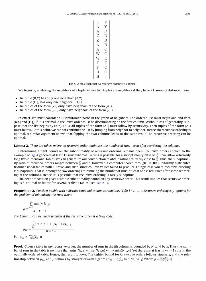
Fig. 4. A table such that no recursive ordering is optimal.


We begin by analyzing the neighbors of a tuple, where two tuples are neighbors if they have a Hamming distance of one:

� The tuple (K,Y) has only one neighbor: (A,Y).� The tuple (H,J) has only one neighbor: (H,C).� The tuples of the form (Z,�) only have neighbors of the form (A,�).� The tuples of the form (�, E) only have neighbors of the form (�,C).

In effect, we must consider all Hamiltonian paths in the graph of neighbors. The ordered list must begin and end with(K,Y) and (H,J), if it is optimal. A recursive order must be discriminating on the first column. Without loss of generality, sup-pose that the list begins by (K,Y). Thus, all tuples of the form (A,�) must follow by recursivity. Then tuples of the form (Z,�)must follow. At this point, we cannot continue the list by jumping from neighbor to neighbor. Hence, no recursive ordering isoptimal. A similar argument shows that flipping the two columns leads to the same result: no recursive ordering can beoptimal.

Lemma 2. There are tables where no recursive order minimizes the number of runs—even after reordering the columns.

Determining a tight bound on the suboptimality of recursive ordering remains open. Recursive orders applied to theexample of Fig. 4 generate at least 15 runs whereas 14 runs is possible, for a suboptimality ratio of 15

14. If we allow arbitrarilylong two-dimensional tables, we can generalize our construction to obtain ratios arbitrarily close to 13

12. Thus, the suboptimal-ity ratio of recursive orders ranges between 13

12 and c. However, a computer search through 100,000 uniformly distributedtridimensional tables with 10 rows and six distinct column values failed to produce a single case where recursive orderingis suboptimal. That is, among the row orderings minimizing the number of runs, at least one is recursive after some reorder-ing of the columns. Hence, it is possible that recursive ordering is rarely suboptimal.

The next proposition gives a simple suboptimality bound on any recursive order. This result implies that recursive order-ing is 3-optimal or better for several realistic tables (see Table 1).

Proposition 2. Consider a table with n distinct rows and column cardinalities Ni for i = 1, . . . , c. Recursive ordering is l-optimal forthe problem of minimizing the runs where

l ¼

Pcj¼1

minðn;N1;jÞ

nþ c � 1:

The bound l can be made stronger if the recursive order is a Gray code:

lGC ¼

Pcj¼1

minðn;1þ ðNj � 1ÞN1;j�1Þ

nþ c � 1:

but lGC >miniðNi�1Þ

miniðNiÞl

Proof. Given a table in any recursive order, the number of runs in the ith column is bounded by N1,iand by n. Thus the num-ber of runs in the table is no more than min (N1,n) + min(N1,2,n) + � � � + min(N1,c,n). Yet there are at least n + c � 1 runs in theoptimally-ordered table. Hence, the result follows. The tighter bound for Gray-code orders follows similarly, and the rela-tionship between lGC and l follows by straightforward algebra (lGC >

Pcj¼1 minðbn; bN1;jÞ where b ¼ miniðNiÞ�1

miniðNiÞ). h

Fig. 5. Table built from graph on the left. There are h copies of the column that begins 10 . . . and the column that begins with 11 . . .


As an example, consider the list of all dates (month, day, year) for a century (N1 = 12,N2 = 31,N3 = 100, n = 12 � 31 � 100):then l � 1.01 so that lexicographic sorting is within 1% of minimizing the number of runs. The optimality bound given byProposition 2 is tighter when the columns are ordered in non-decreasing cardinality (N1 6 N2 6 � � � 6 Nc). This fact alone canbe an argument for ordering the columns in increasing cardinality.

4.2. Determining the optimal column order is NP-hard

For lexicographic sorting, it is NP-hard to determine which column ordering will result in least cost under the RUNCOUNT

model, even when the tables have only two values. We consider the following decision problem:Column-Ordering-for-Lex-Runcount (COLR) Given table T with binary values and given integer K, is there a column ordering

such that the lexicographically sorted T has at most K runs?

Theorem 1. COLR is NP-complete.

Proof. Clearly the problem is in NP. Its NP-hardness is shown by reduction from the variant of Hamiltonian Path where thestarting vertex is given [23, GT39]. Given an instance (V,E) of Hamiltonian Path, without loss of generality let v1 2 V be thespecified starting vertex. We construct a table T as follows: first, start with the incidence matrix. Let V = {v1,v2, . . . ,vjVj} andE = {e1,e2, . . . ,em}. Recall that this matrix has a column for each edge and a row for each vertex; ai,j = 1 if edge ej has vertex vi

as an endpoint and otherwise ai,j = 0. Vertex v1 corresponds to the first row. We prepend and append a row of zeros to theincidence matrix. Next we prepend h columns with values 10jVj+1 (i.e., 100 . . .0) and h columns with 110jVj; see Fig. 5 for anexample. The value of h is ‘‘large’’; we compute the exact value later.

We show the resulting instance, with table T and bound K = 4h + 3(jVj � 1) + 5(m � jVj + 1), satisfies the requirements forCOLR if and only if (V,E) contains a Hamiltonian path starting at v1.

First, suppose that we have a suitable Hamiltonian path in (V,E). Let �i 2 E be the ith edge along this path. Edge �1 isincident upon v1.

Reorder the columns of T: leave the first 2h columns in their current order. Next, place the columns corresponding to �i inorder �1,�2, . . . ,�jVj�1. The remaining columns follow in an arbitrary order. See Fig. 6, where it is apparent that the constructedtable is already lexicographically sorted.3 Also, the first 2h columns have 2 runs each, and the jVj � 1 columns for �i havethree runs each (each has the value 0i110jVj�i). The remaining m � jVj + 1 columns have five runs each: all patterns withadjacent ones have been used (and there are no duplicates); hence, all remaining patterns are of the form 0+10+10+. Thus thebound is met.

Next, suppose T satisfies the requirements of COLR with the given bound K = 4h + 3(jVj � 1) + 5(m � jVj + 1). We show thisimplies (V,E) has a Hamiltonian path starting with v1.

If h is large enough, we can guarantee that the first two rows have not changed their initial order. This is enforced by the2h columns that were initially placed leftmost. Their column values must end with 0 (the row of zeros is always last afterlexicographic sorting ). If we analyze the RUNCOUNT cost of these columns, they cost 4h when the first two rows remain in theirinitial order, otherwise they cost 5h or 6h. If h is large enough, this penalty will outweigh any possible gain from having acolumn order that, when sorted, moves the first two rows.

Knowing the first row, we deduce that every column begins with a one if it is one of the 2h columns, but it begins with azero in every remaining column. We now focus on these remaining columns, which correspond to edges in E. Since eachcolumn value begins and ends with zero and has exactly two ones, its pattern is either 0+110+ (3 runs) or 0+10+10+ (5 runs).The specified RUNCOUNT bound implies that we must have jVj � 1 columns with 3 runs. The edges for these columns form thedesired Hamiltonian path that starts at v1.

3 We sort with 1 ordered before 0.

Fig. 6. A lexicographically sorted table with the required RUNCOUNT bound is obtained from the Hamiltonian path consisting of edges e1, e4, e2, e6.


To finish, we must choose h such that the penalty (for choosing a column ordering that disrupts the order of the first tworows after lexicographic sorting) exceeds any possible gain. The increased cost from 4h is at least 5h, a penalty of at least h.An upper bound on the gain from the other columns is 3m because the RUNCOUNT is no more than 5m and cannot be decreasedbelow 2m. Choose h = 3m + 1. h

This result can be extended to the reflected Gray-code order and, we conjecture, to all recursive orders. A related problemtries to minimize the maximum number of runs in any table column. This problem is also NP-hard (see Appendix D).

Moreover, given a very large number of rows, it might impractical to try more than one column order. Indeed, evaluatingeach new solution implies sorting the table, a potentially expensive step. Thus, heuristics which only consider a few easilycomputed statistics, such as cardinality, are preferable.

5. Increasing-cardinality-order minimizes runs

Consider a sorted table. The table might be sorted in lexicographic order or in reflected Gray-code order. Can we provethat sorting the columns in increasing cardinality is a sensible heuristic to minimize the number of runs? We consider ana-lytically two cases: (1) complete tables and (2) uniformly distributed tables.

5.1. Complete tables

Consider a c-column table with column cardinalities N1,N2, . . . ,Nc. A complete table is one where all N1,c possible tuples arepresent. In practice, even if a table is not complete, the projection on the first few columns might be complete.

Using a lexicographic order, a complete table hasPc

j¼1N1;j runs, hence the RUNCOUNT is minimized when the columns areordered in non-decreasing cardinality: Ni 6 Ni+1 for i = 1, . . . ,c � 1. Using Gray-code ordering, a complete table has onlyc � 1 + N1,c runs (the minimum possible) no matter how the columns are ordered. Hence, for Gray-code, the RUNCOUNT of com-plete tables is not sensitive to the column order.

Somewhat artificially, we can create a family of recursive orders for which the RUNCOUNT is not minimized over completetables when the columns are ordered in increasing cardinality. Consider the following family: ‘‘when N1 is odd, use reflectedGray code order. Otherwise, use lexicographic order.’’ For N1 = 2 and N2 = 3, we have 8 runs using lexicographic order. WithN1 = 3 and N2 = 2, we have 7 runs using any recursive Gray-code order. Hence, we cannot extend our analysis to all families ofrecursive orders from Gray-code and lexicographic orders. Nevertheless, if we assume that all column cardinalities are large,then the number of runs tends to N1,c and all column orders become equivalent.

The benefits of Gray-code orders—all Gray-code orders, not just recursive Gray-code orders—over lexicographic orders aresmall for complete tables having high cardinalities as the next proposition shows (see Fig. 7).

Proposition 3. Consider the number of runs in complete tables with columns having cardinality N. The relative benefit of Gray-code orders over lexicographic orders grows monotonically with c and is at most 1/N.

Proof. The relative benefits of Gray-code sorting for complete tables with all columns having cardinality N isNcþ1�1

N�1 �1�ðNcþc�1ÞNcþ1�1

N�1 �1.

As c grows, this quantity converges to 1/N from below. h

5.2. Uniformly distributed case

We consider tables with column cardinalities N1,N2, . . .Nc. Each of the N1,c possible tuples is present with probability p.When p = 1, we have complete tables.

For recursive orders over uniformly distributed tables, knowing how to compute the expected number of runs in the sec-ond column of a two-column table is almost sufficient to analyze the general case. Indeed, given a 3-column table, the secondcolumn behaves just like the second column in 2-column table with p 1� ð1� pÞN3 . Similarly, the third column behavesjust like the second column in a 2-column table with N1 N1N2 and N2 N3.

0

5

10

15

20

25

30

35

40

45

50

2 3 4 5 6 7 8 9 10

Rel

ativ

e be

nefi

ts o

f G

ray-

code

sor

ting

(%)

Number of columns (c)

N=2N=10

N=100

Fig. 7. Relative benefits of Gray-code sorting against lexicographic orders for complete c-column table where all column cardinalities are N.


This second column is divided into N1 blocks of N2 tuples, each tuple having a probability p of being present. The expectednumber of tuples present in the table is N1N2p. However, N1 N2p is an overestimate of the number of runs in the second col-umn. We need to subtract the expected number of seamless joins between blocks: two blocks have a seamless join if the firstone terminates with the first value of the second block. The expected number of seamless joins is no larger than the expectednumber of non-empty blocks minus one: N1qN2

� 1 where qN2� 1� ð1� pÞN2 . While for complete tables, all recursive Gray-

code orders agree on the number of runs and seamless joins per column, the same is not true for uniformly distributed tables.Different recursive Gray-code orders have different expected numbers of seamless joins.

Nevertheless, we wish to prove a generic result for tables having large column cardinalities (Ni� 1 for all i’s). Consider atwo-column table having uniform column cardinality N. For any recursive order, the expected number of seamless joins isless than NqN. However, the expected sum of the number of runs and seamless joins is NqN in the first column and N2p in thesecond, for a total of NqN + N2p. For a fixed table density, the ratio NqN/(NqN + N2p) goes to zero as 1/N since qN ? 1 expo-nentially. Hence, for tables having large column cardinalities, the expected number of seamless joins is negligible comparedto the expected number of runs. The following lemma makes this result precise.

Lemma 3. Let Si and Ri be the expected number of seamless joins and runs in column i. For all recursive orders, we have

Pci¼1

Si

Pci¼1

Si þPci¼1

Ri

61

mink2f1;2;...;cg

Nk

over uniformly distributed tables.

Proof. Column i + 1 has an expected total of runs and seamless joins of Siþ1 þ Riþ1 ¼ N1;iþ1qNiþ2 ...Nc. It has less than N1;iqNiþ1 ...Nc

seamless joins. We can verify that qNiþ1 ...Nc6 qNiþ2 ...Nc

for all p 2 [0,1]. Thus Si+1/(Si+1 + Ri+1) 6 1/Ni+1.Hence, we have NiSi 6 Si + Ri. This implies that mink2{1, 2, . . . , c}NkSi 6 Si + Ri. Therefore, we have mink2f1;2;...;cgNk

Pci¼1Si 6Pc

i¼1Si þPc

i¼1Ri which proves the result. h

Therefore, for large column cardinalities, we can either consider the number of runs, or the sum of the runs and seamlessjoins. In this context, the next proposition shows that it is best to order columns in increasing cardinality.

Proposition 4. The expected sum of runs and seamless joins is the same for all recursive orders. Moreover, it is minimized overuniformly distributed tables if the columns are sorted by increasing cardinality.

Proof. For all recursive orders, the expected number of runs and seamless joins for columns i and i + 1 is N1;iqNiþ1 ��Ncþ

N1;iþ1qNiþ2 ��Nc. The second term—corresponding to column i + 1—is invariant under a permutation of columns i and i + 1.

We focus our attention on the first term: N1;iqNiþ1 ��Nc. After permuting i and i + 1, it becomes N1;i�1Niþ1qNiNiþ2 ��Nc

.To simplify the notation, rewrite qNiþ1 ��Nc

and qNiNiþ2 ��Ncas qNiþ1

and qNiby substituting qNiþ2 ��Nc

for p and let i = 1. Thus, wecompare N1qN2

and N2qN1.

To prove the result, it is enough to show that N1qN2< N2qN1

implies N1 < N2 for p 2 (0,1]. Suppose that it is not the case: itis possible to have N1qN2

< N2qN1and N1 > N2. Pick such N1,N2. Let x = 1 � p, then N1qN2

� N2qN1is N1ð1� xN2 Þ � N2ð1� xN1 Þ.


The polynomial is positive for x = 0 since N1 > N2. Because N1qN2< N2qN1

is possible (for some value of x), the polynomialmust be negative at some point in (0,1), hence it must have a root in (0,1). However, the polynomial has only 3 terms so thatit cannot have more than 2 positive roots (e.g., by Descartes’ rule of signs). Yet it has a root of multiplicity two at x = 1: afterdividing by x � 1, we get N1ð1þ xþ � � � þ xN2�1Þ � N2ð1þ xþ � � � þ xN1�1Þwhich is again zero at x = 1. Thus, it has no such rootand, by contradiction, N1qN2

6 N2qN1implies N1 6 N2 for p 2 (0,1]. The proof is concluded. h

Theorem 2. Given

1. the expected number of runs R" in a table sorted using any recursive order with an ordering of the column in increasing car-dinality and

2. Roptimal, the smallest possible expected number of runs out of all possible recursive orders on the table (with the columns orderedin any way),

then

R" � Roptimal

R"6

1min

k2f1;2;...;cgNk

over uniformly distributed tables. That is, for large column cardinalities—mink 2 {1, 2, . . . , c}Nk is large— sorting a table recursivelywith the columns ordered in increasing cardinality is asymptotically optimal.

Proof. Whenever a P b, then 1 � a 6 1 � b. Applying this idea to the statement of Lemma 3, we have

1�

Pci¼1

Si

Pci¼1

Si þPci¼1

Ri

P 1� 1min

k2f1;2;...;cgNk

or

Xc

i¼1

Ri Pmin

k2f1;2;...;cgNk � 1

mink2f1;2;...;cg

Nk

Xc

i¼1

Si þXc

i¼1

Ri

!:

Let S" and Soptimal be the expected number of seamless joins corresponding to R" and Roptimal. We have

Roptimal Pmin

k2f1;2;...;cgNk � 1

mink2f1;2;...;cg

NkðRoptimal þ SoptimalÞP

mink2f1;2;...;cg

Nk � 1

mink2f1;2;...;cg

NkðR" þ S"Þ by Proposition 4

Pmin

k2f1;2;...;cgNk � 1

mink2f1;2;...;cg

NkR"

from which the result follows. h

From this theorem, we can conclude that—over uniformly distributed tables having large column cardinalities—sortinglexicographically with the column ordered in increasing cardinality is as good as any other recursive sorting.

The expected benefits of seamless joins are small, at least for uniformly distributed tables. Yet they cause runs from dif-ferent columns to partially overlap. Such partial overlaps might prevent some computational optimizations. For this reason,Bruno [10] avoids seamless joins in RLE-compressed columns: each seamless join becomes the start of a new run. In thismodel, Proposition 4 already shows that ordering the columns in increasing cardinality minimizes the expected numberof runs—for uniformly distributed tables.

5.2.1. Best column order for lexicographic sortingWhile Theorem 2 states that the best column ordering—for all recursive orders—is by increasing cardinality, the result is

only valid asymptotically (for large column cardinalities). For the lexicographic order, we want to prove that the best columnordering is by increasing cardinality, irrespective of the column cardinalities.

The N1 blocks in the second column of a lexicographically ordered are ordered from 1 to N2. Let P�N2 be the probabilitythat any two non-empty such blocks have a seamless join. The probability that the first x tuples in a block are not presentwhereas the x + 1th tuple is present is ð1� pÞxp=ð1� ð1� pÞN2 Þ. To obtain a seamless join, we need a run of precisely N2 � 1


missing tuples, and it can begin anywhere between the second possible tuple in the first block and the first possible tuple in

the second block. (See Fig. 8a.) Hence, we have P�N2 ¼N2p2ð1�pÞN2�1

ð1�ð1�pÞN2 Þ2¼ N2p2ð1�qN2

Þð1�pÞq2

N2

. Let P�N2 ;p0 and qN2 ;p0be P�N2 and qN2

with p0

substituted in place of p.To prove that ordering the columns by increasing cardinality minimizes the number of runs, it is enough to prove that

permuting the columns two-by-two, so as to put the column with lesser cardinality first, never increases the number of runs.To prove this result, we need the following technical lemma.

Lemma 4. For 1 6 N2 < N3 6 30 and 0 < p 6 1, we have

4 We

ð1� P�N3 ÞqN3N2 � P�N2 ;qN3

qN2 ;qN3< ð1� P�N2 ÞqN2

N3 � P�N3 ;qN2qN3 ;qN2

:

Proof. Observe that 1� qN3¼ ð1� pÞN3 and qN2 ;qN3

¼ 1� ð1� pÞN2N3 ¼ qN2N3. To prove the result, we show that

� For p sufficiently close to 1, the result holds.� We can turn the inequality into a polynomial in p with no root in (0,1).

The first item is easy: taking the limit as p ? 1 on both sides of the inequality, we get N2 < N3. To conclude the proof, wehave to show that ð1� P�N3 ÞqN3

N2 � P�N2 ;qN3qN2 ;qN3

� ð1� P�N2 ÞqN2N3 þ P�N3 ;qN2

qN3 ;qN2is never zero for p 2 (0,1). We

multiply this quantity by qN2N3. We proceed to show that the result is a polynomial.

Since 1 � zN = (1 � z)(1 + z + � � � + zN�1), we have that the polynomial qN2N3is divisible by both qN2

and qN3by respectively

setting z ¼ ð1� pÞN2 and z ¼ ð1� pÞN3 . Hence, ð1� P�N3 ÞqN3qN2N3

and ð1� P�N2 ÞqN2qN2N3

are polynomials.

We also have that P�N2 ;qN3qN2 ;qN3

¼N2q2

N3ð1�qN3

ÞN2�1

qN2N3and similarly for P�N3 ;qN2

qN3 ;qN2so that ðP�N2 ;qN3

qN2 ;qN3�

P�N3 ;qN2qN3;qN2

ÞqN2N3is a polynomial.

Hence, for any given N2 and N3, we can check that the result holds by applying Sturm’s method [7] to the polynomial overthe interval (0,1]. Because there is no root at p = 1, we have to check that the total root count over (0,1] is always zero. Weproved this result using a computer algebra system (see Appendix B) for values of N2 and N3 up to 30. This concludes theproof. h

There are N1 � 1 pairs of blocks immediately adjacent, N1 � 2 pairs of blocks separated by a single block, and so on. Hence,

the expected number of seamless joins in the second column is4 SlexicoN1 ;N2

¼ P�N2q2N2

PN1�2k¼0 ðN1 � 1� kÞð1� qN2

Þk or SlexicoN1 ;N2

¼P�N2 ðqN2

N1 þ ð1� qN2ÞN1 � 1Þ ¼ P�N2qN2

N1 þ � for j�j 6 1.

Proposition 5. Consider a table with c independent and uniformly distributed columns having cardinalities N1,N2, . . . ,Nc (let2 6 Ni 6 Ni+1 6 30 for i = 1, . . . , c � 1). We can sort the table by lexicographic order according to various column orders. The columnorder N1,N2, . . . ,Nc minimizes the number of column runs—up to a term no larger than c in absolute value.

Proof. Define T lexicoN1 ;N2 ;qN3

¼ N1N2qN3� P�N2 ;qN3

qN2 ;qN3N1 as the number of expected number of runs—up to a constant term no

larger than one in absolute value—in the second column of a 3-column table with cardinalities N1,N2,N3 and uniform distri-

bution. Define T lexicoN1N2 ;N3 ;p

; T lexicoN1 ;N3 ;qN2

and T lexicoN1N3 ;N2 ;p

similarly. It is sufficient to prove that T lexicoN1 ;N2 ;qN3

þ T lexicoN1N2 ;N3 ;p

6 T lexicoN1 ;N3 ;qN2

þ

T lexicoN1N3 ;N2 ;p

whenever N2 6 N3, irrespective of the value of N1 (allowing N1 > N3). We have

T lexicoN1 ;N2 ;qN3



qN2 ;qN3N1 þ N1N2N3p� P�N3qN3

N1N2

¼ ð1� P�N3 ÞqN3N1N2 � P�N2 ;qN3

qN2 ;qN3N1 þ N1N2N3p

6 ð1� P�N2 ÞqN2N1N3 � P�N3 ;qN2

qN3 ;qN2N1 þ N1N2N3p ðby Lemma 4Þ


qN3 ;qN2N1 þ N1N2N3p� P�N2qN2

N1N3 ¼ T lexicoN1 ;N3 ;qN2


:

This proves the result. h

We conjecture that a similar result would hold for all values of Ni larger than 30. Given arbitrary values of N1, N2, . . . ,Nc,we can quickly check whether the result holds using a computer algebra system.

5.2.2. Best column order for reflected Gray-code sortingFor the reflected Gray-code order, we want to prove that the best column ordering is by increasing cardinality, irrespec-

tive of the column cardinalities. Blocks in reflected Gray-code sort are either ordered from 1 to N2, or from N2 to 1. When two

use the identityPN�2

k¼0 ðN � 1� kÞxk ¼ ð1�xÞNþxN�1ð1�xÞ2

.


non-empty blocks of the same type are separated by empty blocks, the probability of having a seamless join is P�N2 . Other-

wise, the probability of seamless join is PlN2 ¼p2þð1�pÞ2p2þ��þð1�pÞ2N2�2p2

ð1�ð1�pÞN2 Þ2¼ p2ð1�ð1�pÞ2N2 Þð1�ð1�pÞN2 Þ2ð1�ð1�pÞ2Þ

for p 2 (0,1).

There are N1 � 1 pairs of blocks immediately adjacent and with opposite orientations (e.g., from 1 to N2 and then from N2

to 1; see Fig. 8b), N1 � 2 pairs of blocks separated by a single block and having identical orientations, and so on. Hence, the

expected number of seamless joins is PlN2q2N2

PbðN1�1Þ=2ck¼0 ðN1 � 1� 2kÞð1� qN2

Þ2k þ P�N2q2N2

PbðN1�3Þ=2ck¼0 ðN1 � 2� 2kÞ

ð1� qN2Þ2kþ1.

We want a simpler formula for the number of runs, at the expense of introducing an error of plus or minus one run. Soconsider the scenario where we have an infinitely long column, instead of just N1 blocks. However, we count only the num-ber of seamless joins between a block in the first N1 blocks and a block following it. Clearly, there can be at most one extraseamless join, compared to the number of seamless joins within the N1 blocks.

We have the formula xP1

k¼0ð1� xÞ2k ¼ x1�ð1�xÞ2

¼ 12�x. Hence, this new number of seamless joins is Sreflected

N1 ;N2¼

PlN2q2N2

P1k¼0N1ð1� qN2

Þ2k þ P�N2q2N2

P1k¼0N1ð1� qN2

Þ2kþ1 ¼ PlN2qN2

N1

2�qN2þ P�N2

qN2ð1�qN2

ÞN1

2�qN2.

Let kreflectedN2

¼ PlN2þð1�qN2

ÞP�N22�qN2

, then SreflectedN1 ;N2

¼ kreflectedN2

qN2N1.

Lemma 5. The function 1�xN2N3

1�xN3is a real polynomial in x for all positive integers N2,N3.

Lemma 6. If 2 6 N2 < N3 6 30, then

Fig. 8.empty

ð1� kreflectedN3

ÞqN3N2 � kreflected

N2 ;qN3qN2 ;qN3

< ð1� kreflectedN2


N3 ;qN2qN3 ;qN2

:

Proof. The proof is similar to the proof of Lemma 4. We want to show that

� For some value of p in (0,1), the result holds.� We can turn the inequality into a polynomial in p with no root in (0,1).

The first item follows by evaluating the derivative of both sides of the inequality at p = 1. (Formally, our formula is definedfor p 2 (0,1), so we let the values and derivatives of our functions at 1 be implicitly defined as their limit as p tends to 1.) For

all N P 2 and at p = 1, we have that dPlNdp ¼ 2, dP�N

dp ¼ 0; dqNdp ¼ 0, and dkreflected

Ndp ¼ 2; moreover, we have qN = 1 and kreflected

N ¼ 1 at

p = 1. The derivatives of PlN;qN0 ; P�N;qN0 and kreflectedN;qN0 are also zero for all N,N

0P 2 at p = 1. Hence, the derivative of the left-

hand-side of the inequality at p = 1 is �2N2 whereas the derivative of the right-hand-side is �2N3. Because N3 > N2 andequality holds at p = 1, we have that the left-hand-side must be smaller than the right-hand-side at p = 1 � n for somesufficiently small n > 0.

Two consecutive non-empty blocks and the number of missing tuples needed to form a seamless join. The last figure shows the pattern where y � 1blocks separate the two non-empty blocks, and the count sequence in the second block starts at s = 1 + (�ymodN2).


To conclude the proof, we have to show that the value ð1� kreflectedN3


N2 ;qN3qN2 ;qN3

� ð1� kreflectedN2

ÞqN2N3þ

kreflectedN3 ;qN2

qN3 ;qN2is never zero for p 2 (0,1). We multiply this quantity by ð2� qN2N3

ÞqN2N3and call the result !. We first show

that ! is a polynomial.

Because PlN3q2

N3and P�N3q2

N3are polynomials (respectively p2 þ ð1� pÞ2p2 þ � � � þ ð1� pÞ2N2�2p2 and N2p2ð1� pÞN2�1), we

have that kreflectedN3

can be written as a polynomial divided by ð2� qN3Þq2

N3. Hence, kreflected

N3qN3ð2� qN2N3

ÞqN2N3is a polynomial

timesð2�qN2N3

ÞqN2N3ð2�qN3

ÞqN3. In turn, this fraction is 1�ð1�pÞ2N2N3

1�ð1�pÞ2N3which is a polynomial by Lemma 5. Hence, kreflected

N3qN3ð2� qN2N3

ÞqN2N3is

a polynomial. By symmetrical arguments, kreflectedN2

qN2ð2� qN2N3

ÞqN2N3is also a polynomial.

Recall that qN2 ;qN3¼ qN2N3

. We have that kreflectedN2 ;qN3

is a polynomial divided by ð2� qN2N3Þq2

N2N3. Hence, it is immediate that

kreflectedN2 ;qN3

qN2 ;qN3multiplied by ð2� qN2N3

ÞqN2N3is polynomial, merely by canceling the terms in the denominator. A

symmetrical argument applies to kreflectedN3;qN2

qN3 ;qN2.

Hence, ! is a polynomial. As in Lemma 4, for any given N2 and N3, we can check that there are no roots by applyingSturm’s method to the polynomial over the interval (0,1]. Because there is a root at p = 1, it is sufficient to check that the totalroot count over (0,1] is always one. (Alternatively, we could first divide the polynomial by x � 1 and check that there is noroot.) We proved this result using a computer algebra system (see Appendix B). This concludes the proof. h

Proposition 6. Consider a table with c independent and uniformly distributed columns having cardinalities N1,N2, . . . ,Nc (let2 6 Ni 6 Ni+1 6 30 for i = 1, . . . , c � 1). We can sort the table by reflected Gray-code order according to various column orders.The column order N1,N2, . . . ,Nc minimizes the number of column runs—up to a term no larger than c in absolute value.

Proof. The proof is similar to Proposition 5, see Appendix C. h

6. Experiments

To complete the mathematical analysis, we ran experiments on realistic data sets. We are motivated by the followingquestions:

� For columns with few columns, is recursive sorting nearly optimal? (Section 6.3)� How likely is it that alternative column order are preferable to the increasing-cardinality order? (Section 6.4)� How significant can the effect of the column order be? Are reflected Gray-code orders better than lexicographical orders?

(Section 6.5)� How does an Hilbert order compare to lexicographical orders? (Section 6.6)� How large is the effect of skew and column dependency? (Section 6.8)� Do our results extend to other column-compression techniques? (Section 6.9)

6.1. Software

We implemented the various sorting techniques using Java and the Unix command sort. For all but lexicographic order-ing, hexadecimal values were prepended to each line in a preliminary pass over the data, before the command sort wascalled. (This approach is recommended by Richards [51].) Beside recursive orders, we also implemented sorting by CompactHilbert Indexes (henceforth Hilbert) [26]—also by prepending hexadecimal values. By default, we order values within col-umns alphabetically.

6.2. Realistic data sets

We used five data sets (see Table 1) representative of tables found in applications: Census-Income [29], Census1881 [50],DBGEN [57], Netflix [43] and KJV-4grams [39]. The Census-Income table has 4 columns: age, wage per hour, dividends fromstocks and a numerical value5 found in the 25th position of the original data set. The respective cardinalities are 91, 1240, 1478and 99800. The Census1881 came from a publicly available SPSS file 1881_sept2008_SPSS.rar [50] that we converted to a flatfile. In the process, we replaced the special values ‘‘ditto’’ and ‘‘do.’’ by the repeated value, and we deleted all commas withinvalues. The column cardinalities are 183, 2127, 2795, 8837, 24278, 152365, 152882. For DBGEN, we selected dimensions ofcardinality 7, 11, 2526 and 400000. The Netflix table has 4 dimensions: UserID, MovieID, Date and Rating, with cardinalities480189, 17770, 2182, and 5. Each of the four columns of KJV-4grams contains roughly 8 thousand distinct stemmed words:8246, 8387, 8416, and 8504.

5 The associated metadata says this column should be a 10-valued migration code.

Table 1Characteristics of data sets used.

Rows Distinct rows ColsP

ini Size l

Census-Income 199523 178867 4 102609 2.96 MB 2.63Census1881 4277807 4262238 7 343422 305 MB 5.09DBGEN 13977980 11996774 4 402544 297 MB 1.02Netflix 100480507 100 480507 4 500146 2.61 GB 2.00KJV-4grams 877020839 363412308 4 33553 21.6 GB 2.19


Table 1 also gives the suboptimality factor l from Proposition 2. For DBGEN, any recursive order minimizes the number ofruns optimally—up to a factor of 1%. For Netflix and KJV-4-grams, recursive ordering is 2-optimal. Only for Census1881 is thebound on optimality significantly weaker: in this instance, recursive ordering is 5-optimal.

6.3. Recursive sorting is ‘‘safe’’ for low dimensionality

Since our 7-dimensional data set yields a much looser bound than the 4-dimensional data sets, we investigate the rela-tionship between l and the number of dimensions. Rather than use our arbitrarily chosen low-dimensional projections, werandomly generated many projections (typically 1000) of each original data set, computed l for each projection, thenshowed the l values for each dimensionality (i.e., all l values for 3-dimensional projections were averaged and reported;likewise all l values for 4-dimensional projects were averaged and reported). One difficulty arose: computing l for a pro-jection required the number of distinct rows, and we projected from data sets that are at least a large fraction of ourmain-memory size. Gathering this data exactly appears too expensive. Instead, we computed the projection sizes in a fewpasses over our full data sets, using a probabilistic counting technique due to Cai et al. [13] that was shown by Aouicheand Lemire [6] to have a good performance. As an extra step, we corrected the distinct-row estimates so that they never ex-ceeded the product of column cardinalities. To validate our estimates, we computed exact l values for two smaller data sets(TWEED [18,59] with 52 dimensions and 11 k rows, and another with 13 dimensions and 581 k rows) and observed our aver-age l estimates changed by less than 2%. KJV-4grams and Netflix only had four dimensions, and thus we used TWEED to getanother high-dimensional data set.

Fig. 9a shows that, after about three dimensions, l grew roughly linearly with the number of dimensions: the l formula’smin (n,N1,i)/(n + c � 1) terms would typically approximate 1 for all but the first few dimensions. To illustrate this, we com-puted the expected value of l for projections of uniformly distributed tables with various densities p (see Fig. 9b).

This does not mean that any particular recursive sorting algorithm will be this far from optimal. Our l is an upper boundon suboptimality, so it merely means that we have not given evidence that recursive sorting is necessarily good for higher-dimension data sets. For high-dimensional data sets, there could still be a significant advantage in going beyond lexico-graphic sorting or other recursive sorting approaches. However, for 2 or 3 dimensions, our l values show that lexicographicsorting cannot be improved much. Of course, such projections may be nearly complete tables (cf. Section 5.1).

6.4. The column-reordering heuristic is reliable

We showed in Section 5 that reordering the columns in increasing cardinality minimized the expected number ofruns. To assess the reliability of this heuristic, consider a two-dimensional table model where the first column’s values

Fig. 9. Approximate l versus columns, when sampling projections of realistic data sets and synthetic data sets (10-dimensional uniformly distributed tablewith N1 = N2 = � � � = N10 = 10).


are selected uniformly at random from 1 to N1, and the second column’s values are selected uniformly from 1 to N1 + 1:we want the second column to have just barely a higher cardinality than the first. Using this model, we generated100000 100-row tables for each column cardinality N1 from 5 to 30. Of course, we can expect a few missing valueswhen selecting 100 items (with replacement) from N1. Some tables had more missing values in the second column,so we kept only the randomly generated tables where the second column had the higher actual cardinality. We thendetermined the percentage of tables where the increasing-cardinality column-reordering heuristic failed to be at leastas good as the alternative column order (see Fig. 10). The expected relative difference between the cardinalities rangesfrom �1/5 to �1/30. We see that the rate of failure increases as the relative difference between the column cardinalitiesgoes to zero. Even so, the rate of failure is relatively low in this test (less than 3%) despite the small relative difference incardinality.

Although our theoretical results assume uniformity, we have observed that ordering columns in ascending order alsotends to improve results with skewed data. To assess reliability, we repeated the same test for Zipfian-distributed columnsand found the rate of failure was larger. However, it still remained moderate (less than 9%). Moreover, even with Zipfiandistributions, the rate of failure is close to zero when the relative difference between the column cardinalities is large(0.05).

6.5. Column order matters, Gray codes do not

Results for realistic data sets are given in Table 2. For these data sets, there is no noticeable benefit (within 1%) to Graycodes as opposed to lexicographic orders. The only data set showing some benefit (�1%) is KJV-4grams.

Relative to the shuffled case, ordering the columns in increasing cardinality reduced the number of runs by a factor of two(Census and Census1881), three (DBGEN and Netflix) or nine (KJV-4grams). Except for Netflix and KJV-4grams, these gainsdrop to �50% when using the wrong column order (by decreasing cardinality). On Netflix, the difference between the twocolumn orders is a factor of two (2.5 � 108 versus 1.2 � 108).

The data set KJV-4grams appears oblivious to column reordering. We are not surprised given that columns have similarcardinalities and distributions.

Fig. 10. Percentage of failure of the increasing-cardinality column-reordering heuristic.

Table 2RUNCOUNT after sorting various tables using different orderings. The up and down arrows indicate whether the columns where ordered in increasing or decreasingcardinality before sorting. Best results for each data set are in bold.

Table Shuffled Order Lexico. Gray Hilbert

Census-Income 4.6 � 105 ; 3.2 � 105 3.2 � 105 3.4 � 105

" 1.9 � 105 1.9 � 105 3.4 � 105

Census1881 2.7 � 107 ; 1.8 � 107 1.8 � 107 2.0 � 107

" 1.3 � 107 1.3 � 107 2.0 � 107

DBGEN 4.5 � 107 ; 3.3 � 107 3.3 � 107 4.3 � 107

" 1.2 � 107 1.2 � 107 4.3 � 107

Netflix 3.8 � 108 ; 2.5 � 108 2.5 � 108 3.3 � 108

" 1.2 � 108 1.2 � 108 3.3 � 108

KJV-4grams 3.4 � 109 ; 3.9 � 108 3.8 � 108 8.2 � 108

" 3.9 � 108 3.8 � 108 8.2 � 108

Table 3Comparison of Compact Hilbert Indexes with other orderings for a uniformly distributed table (p = 0.01, c = 5) and various column cardinalities. The number ofruns is given in thousands.

Cardinalities Shuffled Lexico. Reflected Gray Modular Gray Hilbert

4,8,16,32,64 47.8 18.9 18.7 18.7 35.364,32,16,8,4 47.8 28.5 28.1 28.2 35.316,16,16,16,16 49.7 23.7 23.3 23.4 35.3


6.6. Compact Hilbert indexes are not competitive

Hilbert is effective at improving the compression of database tables [16,15] using tuple difference coding techniques [44].Moreover, for complete tables where the cardinality of all columns is the same power of two, sorting by Hilbert minimizesthe number of runs (being a Gray code Section 4). However, we are unaware of any application of Hilbert to column-orientedindexes.

To test Hilbert, we generated a small random table (see Table 3) with moderately low density (p = 0.01). The RUNCOUNT re-sult is far worse than recursive ordering, even when all column cardinalities are the same power of 2. In this test, Hilbert iscolumn-order oblivious. We have similar results over realistic data sets (see Table 2). In some instances, Hilbert is nearly asbad as a random shuffle of the table, and always inferior to a mere lexicographic sort. For KJV-4grams, Hilbert is relativelyeffective—reducing the number of runs by a factor of 4—but it is still half as effective as lexicographically sorting thedata.

6.7. The order of values is irrelevant

For several recursive orders (lexicographic and Gray codes), we reordered the attribute values by their frequency—puttingthe most frequent values first [36]. While the number of runs in sorted uniformly distributed tables is oblivious to the orderof attribute values, we may see some benefits with tables having skewed distributions. However, on the realistic data sets,the differences were small—less than 1% on all metrics for recursive ordering.

For Hilbert, reordering the attribute values had small and inconsistent effects. For Census, the number of runs went upfrom 3.4 � 105 to 3.6 � 105 (+6%), whereas for Netflix, it went down from 3.3 � 108 to 3.2 � 108 (�3%). The strongest effectwas observed with KJV-4grams where the number of runs went down from 8.2 � 108 to 7.6 � 108 (�7%). These differencesare never sufficient to make Hilbert competitive.

6.8. Skew and column dependencies reduce the number of runs

We can compute the expected number of runs for uniformly distributed tables sorted lexicographically by the proof ofProposition 5. For Census-Income, we compared this value with the number of runs for all possible column orders (seeFig. 11). Distribution skew and dependencies between columns make a substantial difference: the number of runs wouldbe twice as high were Census-Income uniformly distributed with independent columns.

150000 200000 250000 300000 350000 400000 450000 500000 550000 600000 650000 700000

1234

1243

1324

1342

1423

1432

2134

2143

2314

2341

2413

2431

3124

3142

3214

3241

3412

3421

4123

4132

4213

4231

4312

4321

Num

ber

of r

uns

actualtheory

Fig. 11. Number of runs for the Census-Income data set, including the expected number assuming that the table is uniformly distributed. The columns areindexed from 1 to 4 in increasing cardinality. Hence, the label 1234 means that the columns are in increasing cardinality.

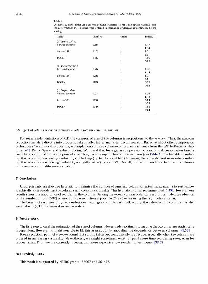
Table 4Compressed sizes under different compression schemes (in MB). The up and down arrowsindicate whether the columns were ordered in increasing or decreasing cardinality beforesorting.

Table Shuffled Order Lexico.

(a) Sparse codingCensus-Income 0.18 ; 0.17

" 0.14Census1881 11.2 ; 8.3

" 8.8DBGEN 14.6 ; 12.9

" 10.3

(b) Indirect codingCensus-Income 0.26 ; 0.20

" 0.15Census1881 12.6 ; 8.3

" 7.9DBGEN 18.9 ; 10.9

" 10.3

(c) Prefix codingCensus-Income 0.27 ; 0.26

" 0.12Census1881 12.6 ; 10.1

" 10.3DBGEN 13.9 ; 13.1

" 10.1


6.9. Effect of column order on alternative column-compression techniques

For some implementations of RLE, the compressed size of the columns is proportional to the RUNCOUNT. Thus, the RUNCOUNT

reduction translate directly into proportionally smaller tables and faster decompression. But what about other compressiontechniques? To answer this question, we implemented three column-compression schemes from the SAP NetWeaver plat-form [40]: Prefix, Sparse and Indirect Coding. We found that for a given compression scheme, the decompression time isroughly proportional to the compressed size. Thus, we only report the compressed sizes (see Table 4). The benefits of order-ing the columns in increasing cardinality can be large (up to a factor of two). However, there are also instances where order-ing the columns in decreasing cardinality is slightly better (by up to 5%). Overall, our recommendation to order the columnsin increasing cardinality remains valid.

7. Conclusion

Unsurprisingly, an effective heuristic to minimize the number of runs and column-oriented index sizes is to sort lexico-graphically after reordering the columns in increasing cardinality. This heuristic is often recommended [1,39]. However, ourresults stress the importance of reordering the columns. Picking the wrong column order can result in a moderate reductionof the number of runs (50%) whereas a large reduction is possible (2–3�) when using the right column order.

The benefit of recursive Gray-code orders over lexicographic orders is small. Sorting the values within columns has alsosmall effects (61%) for several recursive orders.

8. Future work

The first step toward the estimation of the size of column indexes under sorting is to assume that columns are statisticallyindependent. However, it might possible to lift this assumption by modeling the dependency between columns [49,58].

From a practical point of view, we found that sorting tables lexicographically is effective, especially when the columns areordered in increasing cardinality. Nevertheless, we might sometimes want to spend more time reordering rows, even formodest gains. Thus, we are currently investigating more expensive row reordering techniques [33,53].

Acknowledgments

This work is supported by NSERC grants 155967 and 261437.


Appendix A. Table of notation

Notation
Explanation Defined Used in
ri
runs in column i p. 3 Section 1 c number of columns p. 3 Throughout n number of rows p. 5 Throughout Ni Cardinality of column i p. 5 Throughout Ni,j
Qjk¼iNk

p. 5
Throughout
l
recursive sorting is l-optimal for the run minimization problem p. 10 Throughout qNi
Probability that a block of Ni tuples is nonempty
p. 14 Section 5.2 qNi ;p0 same except individual tuples present with probability p0 rather than default p Section 5.2 P�N2 with lexicographic sorting, probability that two nonempty blocks in column 2
seamlessly join
p. 17 Section 5.2
P�N2 ;p0
same except individual tuples present with probability p0 Section 5.2 PlN2
with reflected Gray sorting, probability that two nonempty blocks in column 2seamlessly join

p. 19
Section 5.2
PlN2 ;p0
same except individual tuples present with probability p0 Section 5.2
Appendix B. Maxima computer algebra system code

For completing some of the proofs, we used Maxima version 5.12.0 [54]. Scripts ran during about 49 h on a Mac Pro withtwo double-core Intel Xeon processors (2.66 GHz) and 2 GiB of RAM.

The proof of Lemma 4 uses the following code which ran for 185 min:

r (N2,p):=1-(1-p)⁄⁄N2;

Pdd (N2,p):=N2⁄p⁄⁄2⁄(1-r (N2,p))/((1-p)⁄r (N2,p)⁄⁄2);

P: (1-Pdd (N3,p))⁄r (N3,p)⁄N2- (1-Pdd (N2,p))⁄r (N2,p)⁄N3-Pdd (N2,r (N3,p))⁄r (N2⁄N3,p)+Pdd (N3,r (N2,p))⁄r (N2⁄N3,p);P2:P⁄r (N2⁄N3,p);for n2:2 unless n2 > 30 do

(display (n2),for n3:n2 + 1 unless n3 > 100 do

(nr: nroots (factor (subst ([N2 = n2,N3 = n3],P2)),0,1),if (not (nr = 0)) then display ("ERROR",n2,n3,nr)));

The proof of Lemma 6 uses this code which ran for 46 h:

r (N2,p):=1-(1-p)⁄⁄N2;

Pdd (N2,p):=N2⁄p⁄⁄2⁄(1-r (N2,p))/((1-p)⁄r (N2,p)⁄⁄2);

Pud (N2,p):=p⁄⁄2⁄(2-r (N2,p))/(r (N2,p)⁄(1-(1-p)⁄⁄2));

Lambda (N2,p):=(Pud (N2,p)+(1-r (N2,p))⁄Pdd (N2,p))/(2-r (N2,p));

P: (1-Lambda (N3,p))⁄r (N3,p)⁄N2- (1-Lambda (N2,p))⁄r (N2,p)⁄N3-Lambda (N2,r (N3,p))⁄r (N2⁄N3,p)+Lambda (N3,r (N2,p))⁄r (N2⁄N3,p);P2:P⁄(2-r (N2⁄N3,p))⁄r (N2⁄N3,p);for n2:2 unless n2 > 30 do

(display (n2),for n3:n2 + 1 unless n3 > 100 do

(nr: nroots (factor (subst ([N2 = n2,N3 = n3],P2)),0,1),if (not (nr = 1)) then display ("ERROR",n2,n3,nr)));


Appendix C. Proof of Proposition 6

Proof. Define TreflectedN1 ;N2 ;qN3

¼ N1N2qN3� Sreflected

N1 ;N2 ;qN3where Sreflected

N1 ;N2 ;qN3is defined as Sreflected

N1 ;N2after substituting qN3

for p. Define

kreflectedN2 ;qN3

, TreflectedN1N2 ;N3 ;p, Treflected

N1 ;N3 ;qN2and Treflected

N1N3 ;N2 ;p similarly. As in the proof of Proposition 5, it is sufficient to prove that TreflectedN1;N2 ;qN3

þ

TreflectedN1N2 ;N3 ;p 6 Treflected

N1 ;N3;qN2þ Treflected

N1N3 ;N2;p whenever N2 6 N3, irrespective of the value of N1 (allowing N1 > N3).We have

TreflectedN1 ;N2 ;qN3

þ TreflectedN1N2 ;N3 ;p

¼ N1N2qN3� k reflected

N2 ;qN3qN2 ;qN3

N1 þ N1N2N3p� kreflectedN3

qN3N1N2

¼ ð1� kreflectedN3

ÞqN3N1N2 � k reflected

N2 ;qN3qN2 ;qN3

N1 þ N1N2N3p

6 ð1� kreflectedN2

ÞqN2N1N3 � kreflected

N3 ;qN2qN3 ;qN2

N1 þ N1N2N3pþ kreflectedN2

ðby Lemma 6Þ

¼ N1N3qN2� k reflected

N3 ;qN2qN3 ;qN2

N1 þ N1N2N3p� kreflectedN2

qN2N1N3 ¼ Treflected

N1 ;N3 ;qN2þ Treflected

N1N3 ;N2 ;p:

This proves the result. h

Appendix D. A related NP-completeness result

In Section 4.2 we showed it is NP-hard to order columns so as to minimize the RUNCOUNT value after lexicographic sorting.We now show a related problem is NP-complete.

Column-Ordering-for-Minimax Lexicographic Runcount (COMLR) Given a table T, an ordering on the values found in eachcolumn, and an integer K, is it possible to reorder the columns of the table, such that when the reordered table is lexicograph-ically sorted, no column has more than K runs?

Proposition 7. COMLR is NP-complete.

Proof. Membership in NP is obvious. We show COMLR is NP-hard by reduction from 3SAT [23, LO2]. Suppose our 3SATinstance has variables v1 to vjVj and clauses C1 to Cm. We assume that no clause contains both a variable and its negationbecause such a clause can be removed without affecting satisfiability.

For every variable vi, the COMLR instance has three values that can appear in tables: wi, �wi and 0wi . They are ordered:wi < �wi < 0wi . Moreover, for a 2 fwi; �wi;0wig, b 2 fwj; �wj;0wjg and i – j, we have a < b if and only if i < j.

Two other values are used in the table, +1 and �1 whose orderings with respect to the other values are as expected.We construct a table T, with 3jVj + 2 rows, and with a column for each possible literal and a column for each clause. Hence

T has 2jVj + m columns. We describe the columns from left to right, beginning with the columns for �v1 and v1 (see Fig. 12).Consider the literal column associated with �v1. It begins with a run of length 3 � 1 � 2 with the �1 value. It then

contains �w1; �w1; 0w1 . The remainder of the column is composed of +1. The next column is for v1. It begins and endssimilarly, but in the middle it has w1; 0w1 ; w1. The pairs of columns for the remaining variables then follow. The column for

Fig. 12. Example construction for {c1,c2,c3,c4}, where c1 ¼ fv1; �v2;v3g, c2 ¼ f �v1; �v2; v3g, c3 ¼ f �v1; �v3; v4g, and c4 = {v1,v3,v4}.


�v i begins with a run containing 3i � 2 copies of the �1 value, then has �wi; �wi0wi , whereas the column for vi has wi;0wi ;wi

between the run of �1 and the run of +1. Thus, the left part of the table has blocks of size 3 � 2 arranged diagonally. Abovethe diagonal, we have �1; below the diagonal, we have +1. (Except that there is a row of �1 above everything and a row of+1 below everything.)

To complete the construction, we have one column per clause. Consider a clause {li, lj, lk} where li = vi or li ¼ �v i andsimilarly for lj and lk. Each column begins with �1 and ends with +1. Otherwise, the column copies the column for li withinthe zone of vi, where the zone of variable vi consists of rows 3i � 2, 3i � 1, 3i in the table. The construction is such that nomatter how columns are reordered, a lexicographic sort can rearrange rows only within their zones. Similarly, the columncopies the columns for lj and lk within the zones of vj and vk, respectively. Otherwise, the part of the column that is in thezone of wl (l R {i, j,k}), contains 0wl . See Fig. 12 for the table constructed for ffv1; �v2;v3g; f �v1; �v2;v3g; f �v1; �v3;v4g;fv1;v3;v4gg. Finally, we set the maximum-runs-per-column bound K = jVj + 7.

The construction creates literal columns that cannot have many runs no matter how we reorder columns andlexicographically sort the rows. Consequently these columns always meet the jVj + 7 bound. For clause columns: after anycolumn permutation and lexicographic sorting, a clause column can have at most jVj + 8 runs:

� 2 for the �1 and the +1,� (jVj � 3) for the variables that are not in the clause,� and at most 3 for each of the 3 variables that are in the clause.

Table T can have its columns reordered to have at most jVj + 7 runs per column (after lexicographic sorting), if and only ifthe given instance of 3SAT is satisfiable.

Suppose we have a satisfying truth assignment. If vi is true, permute the columns for �v i and vi. (Otherwise, leave themalone.) After permuting these columns, lexicographic sorting would swap the bottom two rows in the zone for vi. Any clausecontaining vi would find that this swap merges two runs of wi in its column, and thus we would meet the jVj + 7 bound forthat clause’s column. Likewise, if vi is false, leave the two columns in their original relationship. The table as constructed waslexicographically sorted, and any clause containing �v i would continue to have a run of �wi’s and meet the run bound. Since wehave a satisfying truth assignment, every clause column will contain at least one such run.

Conversely, suppose we have permuted table columns such that the lexicographically sorted table has no column withmore than jVj + 7 runs. Because lexicographic sorting is restricted to rearranging rows only within their zones, a clause’scolumn must contain a length-two run of wi or �wi, for some 1 6 i 6 jVj. The construction guarantees that if any clause columncontains a length-two run of wi, then no column contains a length-two run of �wi. Similarly, a length-two run of �wi precludes alength-two run of wi. Moreover, by construction we see that a column containing the length-two run of wi must contain vi.Hence, we set vi to true. Likewise, for any run of �wi we set vi to false. Clearly, this truth setting satisfies the original 3SATinstance. h

References

[1] D. Abadi, S. Madden, M. Ferreira, Integrating compression and execution in column-oriented database systems, in: Proceedings of the 2006 ACMSIGMOD International Conference on Management of Data, ACM, New York, NY, USA, 2006, pp. 671–682.

[2] J. Alber, R. Niedermeier, On multidimensional curves with Hilbert property, Theory of Computing Systems 33 (4) (2000) 295–312.[3] M. Anantha, B. Bose, B. AlBdaiwi, Mixed-radix Gray codes in Lee metric, IEEE Transactions on Computers 56 (10) (2007) 1297–1307.[4] V.N. Anh, A. Moffat, Inverted index compression using word-aligned binary codes, Information Retrieval 8 (1) (2005) 151–166.[5] G. Antoshenkov, Byte-aligned bitmap compression, in: Proceedings of the Conference on Data Compression, IEEE Computer Society, Washington, DC,

USA, 1995, p. 476.[6] K. Aouiche, D. Lemire, A comparison of five probabilistic view-size estimation techniques in OLAP, in: Proceedings of the ACM tenth international

workshop on Data warehousing and OLAP, ACM, New York, NY, USA, 2007, pp. 17–24.[7] S. Barnard, Higher Algebra, Barnard Press, 2008.[8] M. Bassiouni, Data compression in scientific and statistical databases, IEEE Transactions on Software Engineering 11 (10) (1985) 1047–1058.[9] B. Bhattacharjee, L. Lim, T. Malkemus, G. Mihaila, K. Ross, S. Lau, C. McArthur, Z. Toth, R. Sherkat, Efficient index compression in DB2 LUW, Proceedings

of the VLDB Endowment 2 (2009) 1462–1473.[10] N. Bruno, Teaching an old elephant new tricks, in: Conference on Innovative Data Systems Research, 2009.[11] S. Büttcher, C.L.A. Clarke, Index compression is good, especially for random access, in: Proceedings of the Sixteenth ACM Conference on Conference on

Information and Knowledge Management, 2007, pp. 761–770.[12] J. Cai, R. Paige, Using multiset discrimination to solve language processing problems without hashing, Theoretical Computer Science 145 (1–2) (1995)

189–228.[13] M. Cai, J. Pan, Y.-K. Kwok, K. Hwang, Fast and accurate traffic matrix measurement using adaptive cardinality counting, in: Proceedings of the 2005

ACM SIGCOMM Workshop on Mining Network Data, 2005, pp. 205–206.[14] J.-C. Chen, C.-H. Tsai, Conditional edge-fault-tolerant hamiltonicity of dual-cubes, Information Sciences 181 (3) (2011) 620–627.[15] F. Dehne, T. Eavis, B. Liang, Compressing data cube in parallel OLAP systems, Data Science Journal 6 (0) (2007) 184–197.[16] T. Eavis, D. Cueva, A Hilbert space compression architecture for data warehouse environments, Lecture Notes in Computer Science 4654 (2007) 1–12.[17] M.Y. Eltabakh, W.-K. Hon, R. Shah, W.G. Aref, J.S. Vitter, The SBC-tree: an index for run-length compressed sequences, in: Proceedings of the 11th

International Conference on Extending Database Technology: Advances in Database Technology, 2008, pp. 523–534.[18] J.O. Engene, Five decades of terrorism in Europe: The TWEED dataset, Journal of Peace Research 44 (1) (2007) 109–121.[19] C. Faloutsos, Multiattribute hashing using Gray codes, SIGMOD Record 15 (2) (1986) 227–238.[20] J.-F. Fang, The bipancycle-connectivity of the hypercube, Information Sciences 178 (24) (2008) 4679–4687.[21] M. Flahive, Balancing cyclic R-ary Gray codes II, Electronic Journal of Combinatorics 15 (R128) (2008) 1.[22] M. Flahive, B. Bose, Balancing cyclic R-ary Gray codes, Electronic Journal of Combinatorics 14 (R31) (2007) 1.


[23] M.R. Garey, D.S. Johnson, Computers and Intractability: A Guide to the Theory of NP-Completeness, W.H. Freeman, New York, 1979.[24] S.W. Golomb, Run-length encodings, IEEE Transactions on Information Theory 12 (1966) 399–401.[25] S. Haddadi, A note on the NP-hardness of the consecutive block minimization problem, International Transactions in Operational Research 9 (6) (2002)

775–777.[26] C.H. Hamilton, A. Rau-Chaplin, Compact Hilbert indices: Space-filling curves for domains with unequal side lengths, Information Processing Letters 105

(5) (2007) 155–163.[27] H. Haverkort, F. van Walderveen, Locality and bounding-box quality of two-dimensional space-filling curves, Computational Geometry: Theory and

Applications 43 (2010) 131–147.[28] H.J. Haverkort, F. van Walderveen, Four-dimensional Hilbert curves for R-trees, in: Proceedings of the Eleventh Workshop on Algorithm Engineering

and Experiments, 2009, pp. 63–73.[29] S. Hettich, S.D. Bay, The UCI KDD archive, http://kdd.ics.uci.edu (Last checked 01-04-2011) (2000).[30] A.L. Holloway, D.J. DeWitt, Read-optimized databases, in depth, Proceedings of the VLDB Endowment 1 (1) (2008) 502–513.[31] A.L. Holloway, V. Raman, G. Swart, D.J. DeWitt, How to barter bits for chronons: Compression and bandwidth trade offs for database scans, in:

Proceedings of the 2007 ACM SIGMOD International Conference on Management of Data, ACM, New York, NY, USA, 2007, pp. 389–400.[32] B.R. Iyer, D. Wilhite, Data compression support in databases, in: Proceedings of the 20th International Conference on Very Large Data Bases, 1994, pp.

695–704.[33] D. Johnson, S. Krishnan, J. Chhugani, S. Kumar, S. Venkatasubramanian, Compressing large boolean matrices using reordering techniques, in:

Proceedings of the Thirtieth international Conference on Very Large Data Bases, VLDB Endowment, 2004, pp. 13–23.[34] D.S. Johnson, S. Krishnan, J. Chhugani, S. Kumar, S. Venkatasubramanian, Compressing large boolean matrices using reordering techniques, in:

Proceedings of the Thirtieth international Conference on Very Large Data Bases, VLDB Endowment, San Jose, CA, USA, 2004, pp. 13–23.[35] I. Kamel, C. Faloutsos, Hilbert R-tree: An improved R-tree using fractals, in: Proceedings of the 20th International Conference on Very Large Data Bases,

Morgan Kaufmann Publishers Inc., San Francisco, CA, USA, 1994, pp. 500–509.[36] O. Kaser, D. Lemire, Attribute value reordering for efficient hybrid OLAP, Information Sciences 176 (16) (2006) 2304–2336.[37] D.E. Knuth, The Art of Computer Programming, vol. 4, chap. fascicle 2, Addison Wesley, Reading, MA, USA, 2005.[38] H. Lebesgue, Leçons sur l’intégration et la recherche des fonctions primitives: professées au Collège de France, Gauthier-Villars, 1904.[39] D. Lemire, O. Kaser, K. Aouiche, Sorting improves word-aligned bitmap indexes, Data & Knowledge Engineering 69 (1) (2010) 3–28.[40] C. Lemke, K.-U. Sattler, F. Faerber, A. Zeier, Speeding up queries in column stores, in: Data Warehousing and Knowledge Discovery, Lecture Notes in

Computer Science, vol. 6263, Springer, Berlin/Heidelberg, 2010, pp. 117–129.[41] A. Moffat, L. Stuiver, Binary interpolative coding for effective index compression, Information Retrieval 3 (1) (2000) 25–47.[42] A. Moffat, J. Zobel, Self-indexing inverted files for fast text retrieval, ACM Transactions on Information Systems 14 (4) (1996) 349–379.[43] Netflix, Inc., Nexflix Prize, http://www.netflixprize.com (Last checked 01-04-2011) (2007).[44] W. Ng, C. Ravishankar, Block-oriented compression techniques for large statistical databases, IEEE Transactions on Knowledge and Data Engineering 9

(2) (1997) 314–328.[45] R. Niedermeier, K. Reinhardt, P. Sanders, Towards optimal locality in mesh-indexings, Discrete Applied Mathematics 117 (1-3) (2002) 211–237.[46] P. O’Neil, D. Quass, Improved query performance with variant indexes, in: Proceedings of the 1997 ACM SIGMOD International Conference on

Management of Data, 1997, pp. 38–49.[47] G. Peano, Sur une courbe, qui remplit toute une aire plane, Mathematische Annalen 36 (1) (1890) 157–160.[48] A. Pinar, M.T. Heath, Improving performance of sparse matrix-vector multiplication, in: Proceedings of the 1999 ACM/IEEE Conference on

Supercomputing, ACM, New York, NY, USA, 1999. Article No. 30.[49] V. Poosala, Y.E. Ioannidis, Selectivity estimation without the attribute value independence assumption, in: Proceedings of the 23rd International

Conference on Very Large Data Bases, 1997, pp. 486–495.[50] Programme de recherche en démographie historique, PRDH 1881, http://www.prdh.umontreal.ca/census/en/main.aspx, last checked 01-04-2011

(2009).[51] D. Richards, Data compression and Gray-code sorting, Information Processing Letters 22 (4) (1986) 201–205.[52] C. Savage, A survey of combinatorial Gray codes, SIAM Review 39 (1997) 605–629.[53] M. Schaller, Reclustering of high energy physics data, in: Proceedings of the 11th International Conference on Scientific and Statistical Database

Management, IEEE Computer Society, Washington, DC, USA, 1999, pp. 194–203.[54] W. Schelter et al., Maxima, a computer algebra system, http://maxima.sourceforge.net/ (Last checked 01-04-2011) (1998).[55] F. Scholer, H. Williams, J. Yiannis, J. Zobel, Compression of inverted indexes for fast query evaluation, in: Proceedings of the 25th Annual International

ACM SIGIR Conference on Research and Development in Information Retrieval, ACM, New York, NY, USA, 2002, pp. 222–229.[56] M. Stonebraker, D.J. Abadi, A. Batkin, X. Chen, M. Cherniack, M. Ferreira, E. Lau, A. Lin, S. Madden, E. O’Neil, P. O’Neil, A. Rasin, N. Tran, S. Zdonik, C-Store:

a column-oriented DBMS, in: Proceedings of the 31st International Conference on Very Large Data Bases, VLDB Endowment, San Jose, CA, USA, 2005,pp. 553–564.

[57] Transaction Processing Performance Council, DBGEN 2.4.0, http://www.tpc.org/tpch/ (Last checked 01-04-2011) (2006).[58] B.D. Vo, K.-P. Vo, Compressing table data with column dependency, Theoretical Computer Science 387 (3) (2007) 273–283.[59] H. Webb, O. Kaser, D. Lemire, Pruning attribute values from data cubes with diamond dicing, in: Proceedings of the 2008 International Symposium on

Database Engineering & Applications, 2008, pp. 121–129.[60] I.H. Witten, A. Moffat, T.C. Bell, Managing Gigabytes (2nd ed.): Compressing and Indexing Documents and Images, Morgan Kaufmann Publishers Inc.,

San Francisco, CA, USA, 1999.[61] K. Wu, E.J. Otoo, A. Shoshani, Optimizing bitmap indices with efficient compression, ACM Transactions on Database Systems 31 (1) (2006) 1–38.[62] H. Yan, S. Ding, T. Suel, Inverted index compression and query processing with optimized document ordering, in: Proceedings of the 18th International

Conference on World Wide Web, 2009, pp. 401–410.[63] J. Zhang, X. Long, T. Suel, Performance of compressed inverted list caching in search engines, in: Proceeding of the 17th International Conference on

World Wide Web, 2008, pp. 387–396.[64] J. Zobel, A. Moffat, Inverted files for text search engines, ACM Computing Surveys 38 (2) (2006) 6.

http://kdd.ics.uci.edu

http://www.netflixprize.com

http://www.prdh.umontreal.ca/census/en/main.aspx

http://maxima.sourceforge.net/

http://www.tpc.org/tpch/