Renormalization of Discrete Models

without Background

Robert Oeckl∗

Centre de Physique Theorique, CNRS Luminy,13288 Marseille cedex 9, France

CPT-2002/P.446111 December 2002

Abstract

Conventional renormalization methods in statistical physics andlattice quantum field theory assume a flat metric background. Weoutline here a generalization of such methods to models on discretizedspaces without metric background. Cellular decompositions play therole of discretizations. The group of scale transformations is replacedby the groupoid of changes of cellular decompositions. We introducecellular moves which generate this groupoid and allow to define a renor-malization groupoid flow.

We proceed to test our approach on several models. Quantum BFtheory is the simplest example as it is almost topological and the renor-malization almost trivial. More interesting is generalized lattice gaugetheory for which a qualitative picture of the renormalization groupoidflow can be given. This is confirmed by the exact renormalization indimension two.

A main motivation for our approach are discrete models of quantumgravity. We investigate both the Reisenberger and the Barrett-Cranespin foam model in view of their amenability to a renormalization treat-ment. In the second case a lack of tunable local parameters promptsus to introduce a new model. For the Reisenberger and the new modelwe discuss qualitative aspects of the renormalization groupoid flow. Inboth cases quantum BF theory is the UV fixed point.

∗email: oeckl@cpt.univ-mrs.fr

1

Contents

1 Introduction 3

2 Cellular decompositions and moves 6

3 The renormalization groupoid 83.1 Changes of cellular decomposition . . . . . . . . . . . . . . . 83.2 Action of the renormalization groupoid . . . . . . . . . . . . . 9

4 Circuit diagrams 104.1 Basics . . . . . . . . . . . . . . . . . . . . . . . . . . . . . . . 104.2 Key identities . . . . . . . . . . . . . . . . . . . . . . . . . . . 13

5 Discrete gauge theory models 165.1 Quantum BF theory . . . . . . . . . . . . . . . . . . . . . . . 16

5.1.1 Discretization and quantization . . . . . . . . . . . . . 165.1.2 Exact renormalization . . . . . . . . . . . . . . . . . . 18

5.2 Generalized Yang-Mills theory . . . . . . . . . . . . . . . . . . 215.2.1 Discretization and quantization . . . . . . . . . . . . . 215.2.2 Renormalization in general . . . . . . . . . . . . . . . 23

5.3 Exact renormalization in dimension two . . . . . . . . . . . . 25

6 Spin foam models of quantum gravity 266.1 Motivation: BF theory plus constraint . . . . . . . . . . . . . 276.2 The Reisenberger model . . . . . . . . . . . . . . . . . . . . . 276.3 The Barrett-Crane model . . . . . . . . . . . . . . . . . . . . 296.4 An interpolating model . . . . . . . . . . . . . . . . . . . . . 32

7 Discussion and conclusions 34

2

1 Introduction

Renormalization is an essential tool both in condensed matter and high en-ergy physics. It is necessary to make sense of and understand the propertiesof physical models. In the first case and to some extent also in the second,models are often defined as state sums on discretizations of space-time (spinsystems, lattice gauge theory etc.). Renormalization consists then in un-derstanding and controlling the behaviour of a model under changes of thediscretization.

The discretizations of space (or space-time) employed in these models areusually hyper-cubic or other types of regular lattices. This is justified by thefact that the models are defined on a flat metric background. To describe achange in discretization it is thus sufficient to specify a scaling factor. Renor-malization means to tune the fundamental parameters (coupling constantsetc.) of a model in such a way depending on the lattice spacing that suitablephysical observables remain (approximately) unchanged. This is expressedthrough an action of the group of scale transformations (which is referred toas the renormalization group in this context) on the parameter space. Therenormalization group flows are the orbits of this action. A renormalizationgroup fixed point is a model (or a point in parameter space of a model) whichremains invariant under renormalization group (i.e. scale) transformations.This usually implies that it is invariant under all conformal transformations.

The question we investigate in this paper is what renormalization meansfor models defined on discretizations of space-time without any metric back-ground structure. Unsurprisingly, the prime example for such models arenon-perturbative models of quantum gravity. Indeed, after introducing ourgeneral approach such models will be the focus of our investigation.

The first thing to specify is to say what exactly we mean by a discretiza-tion of space-time. This is less trivial than in flat background models as wecan no longer resort to any sort of regular lattice. Furthermore, we wantto respect the global structure of a space-time manifold in an exact senseand allow the inclusion of boundaries (although the latter are not explicitlytreated in the present paper). We use the notion of cellular decomposition,i.e. decomposition as a CW-complex. This includes the notion of simpli-cial decomposition, which is employed in many popular models of quantumgravity. However, cellular decompositions are more general and appear muchbetter suited to handle the problem of renormalization as we shall explain.

Practically every discrete model on a compact topological manifold canbe defined using cellular decompositions. What is more relevant is thatmany models can be naturally defined on arbitrary cellular decompositions.It was shown in [?] that this includes a generalization of lattice gauge theoryand the topological quantum field theories of Turaev-Viro [?, ?] and Crane-Yetter [?].

The second step is to describe changes of discretization and identify a

3

suitable analogue of the renormalization group. In contrast to fixed back-ground models there is no notion of scale or scale transformation and in-deed no notion of global change of discretization at all. Instead, we considerall possible cellular decompositions of a manifold and all possible changesbetween them, i.e. any pair of decompositions. This leads to a groupoidstructure on (the category of) cellular decompositions. This renormaliza-tion groupoid is the analogue of the renormalization group of flat backgroundmodels. Attached to it are notions of refinement and coarsening of cellulardecompositions. The latter expresses the idea of integrating out degrees offreedom.

To get some control on the renormalization groupoid we introduce a setof coarsening moves which we call cellular moves. There are n types ofsuch moves in n dimensions. (One type of move was already introduced in[?] while for the case of dimension three the two others were introduced in[?].) In contrast to the fixed background case changes of discretization canoccur not only locally, but there are even different ways of making a change“at a given place”. We conjecture that any two cellular decompositions arerelated by a sequence of these moves and their inverses. (This was provenfor dimension three in a piecewise linear context in [?].) In particular, thismeans that the moves generate the groupoid.

To allow for a non-trivial renormalization a model in our context musthave local parameters that the renormalization groupoid will act on. Theseare parameters that are associated with certain cells in a cellular decom-position. We define what a local action of the renormalization groupoidmeans.

Note that our treatment of renormalization takes no prejudice as towhether a discrete structure of space-time is really a physical phenomenon(as in condensed matter physics) or a mathematical artifact (as in latticegauge theory). In both situations the methods developed here should beapplicable as is the case for the renormalization methods for flat backgroundmodels.

After setting up the general framework we proceed to discuss the renor-malization of specific models. In general, the identification of suitable ob-servables and the actual renormalization with respect to them is quite a hardproblem. It goes beyond the scope of the present paper where we only aimat demonstrating the workings of our renormalization framework in princi-ple. Instead, we contend ourselves with a renormalization of the partitionfunction. That is, renormalization is to keep the partition function fixedunder changes of cellular decomposition.

All the models we consider are state sum models and can be motivated aspath integral quantizations of field theories. The first two models are discretegauge theories, for which a fairly extensive discussion of renormalization canbe given. The simpler model, quantum BF theory, is almost topological, i.e.almost a renormalization groupoid fixed point. Indeed, we perform the exact

4

renormalization which involves a non-trivial (but rather simple) action of therenormalization groupoid on a global parameter. This non-trivial action canbe considered the origin of the well known anomaly. Removing the anomalyby inserting an appropriate factor leads to a true renormalization groupoidfixed point. The quantum group generalization of this model is the Turaev-Viro TQFT (in dimension three) or the Crane-Yetter TQFT (in dimensionfour), see [?].

The second model is discrete quantum Yang-Mills theory (or latticegauge theory) generalized to cellular decompositions [?]. This cellular gaugetheory can be viewed as arising from turning a metric background (of usualYang-Mills theory) into local parameters of a background-free model. In-deed, these local parameters are necessary ingredients of a theory that isnot at all topological. We discuss general features of the renormalizationgroupoid flow including the ultraviolet and infrared fixed points. For thetwo dimensional case we perform an exact renormalization (suggested bythe exact solvability of lattice gauge theory in two dimensions). It involvesa non-trivial action of the renormalization groupoid on the local parametersand confirms the qualitative picture of the general case.

The further models we consider are spin foam models of Euclidean quan-tum gravity, originally defined on simplicial decompositions. They also de-rive from discrete gauge theories and can be constructed as modificationsof quantum BF theory. For these models we contend ourselves with a dis-cussion of their amenability to a renormalization treatment in our sense.This implies firstly considering the models “as is”, and secondly proposingsuitable modifications.

Necessary requirements for renormalization are the presence of local pa-rameters (as the models are not topological) and their defineability on arbi-trary cellular decompositions. The first model considered in this context isthe Reisenberger model [?]. This has a global parameter which can be easilylocalized. On the other hand there appears to be no obvious generalizationof the model to cellular decomposition. Nevertheless, we are able to sketchsome properties of the renormalization groupoid flow.

The second model of quantum gravity we consider is the Barrett-Cranemodel [?]. While originally defined on simplicial decompositions only our for-mulation extends naturally to arbitrary cellular decompositions (as alreadysuggested by Reisenberger [?]). On the other hand, local tunable parametersare completely absent. This prompts us to propose a new model which in-terpolates between quantum BF theory and the Barrett-Crane model. Thismakes use of a heat kernel operator which in lattice gauge theory interpo-lates between a strong and weak coupling regime. Here the weak couplinglimit corresponds to quantum BF theory (as in lattice gauge theory) whilethe strong coupling limit corresponds to the Barrett-Crane model. Indeed,the renormalization groupoid flow is surprisingly similar to that of cellulargauge theory including an ultraviolet fixed point and an “almost” infrared

5

fixed point (which is the Barrett-Crane model).The formalism we use to express the discussed models is a diagrammatic

one. It is essentially the formalism introduced in [?] to represent morphismsin monoidal categories. We employ here a simplified form adapted to Liegroups and give a self-contained description of it. This diagrammatics isstrongly related to the connection formulation of discrete gauge models whileit also easily translates into the spin foam formalism (see Section 8.1 in [?]).Moreover, in its general form it includes the supergroup and the quantumgroup case. This implies that much of our treatment of concrete models inthis paper generalizes directly to supergroups and quantum groups as gaugegroups (see in particular Section 4.2 in [?]).

The first part of the paper presents our proposal of a framework forrenormalization. In Section 2 cellular decompositions and the cellular movesare introduced while Section 3 contains the basic notions of renormalizationgroupoid and its action. The second part of the paper is devoted to appli-cations. It starts with Section 4 which serves as a brief review of the dia-grammatic language employed in the following. Section 5 treats the renor-malization of quantum BF theory and of cellular gauge theory. Section 6deals with the question of renormalization for spin foam models of quantumgravity. Finally, Section 7 presents some conclusions.

2 Cellular decompositions and moves

In this section we give the necessary background on cellular decompositionsand introduce the cellular moves. The former serve as our definition of“discretization of a space”, while the latter serve to formalize and control“changes of discretization”.

Roughly speaking, a cellular decomposition is a division of a compactmanifold into open balls, called cells. For a manifold of dimension n thereare not only cells of dimension n but also cells of lower dimension, fillingthe gaps between the higher dimensional cells, down to dimension 0-cells(points). More precisely, a cellular decomposition is a presentation of amanifold as a CW-complex. This can also be formalized as in the followingdefinition.

Definition 2.1. Let M be a compact manifold of dimension n. A cellulardecomposition of M is a presentation of M as the disjoint union of finitelymany sets

M =⋃

k∈0,...,n,iCk

i

with the following properties: (a) Cki , called a k-cell, is homeomorphic to an

open ball of dimension k. (An open ball of dimension 0 is defined to be a

6

point.) (b) The boundary of each cell is contained in the union of the cellsof lower dimension. Here, the boundary ∂C of a cell C is defined to be theclosure of C in M with C removed.

Next, we introduce the concepts of refinement and its opposite, coars-ening. This is rather intuitive and the definition straightforward.

Definition 2.2. Let M be a compact manifold with cellular decompositionsC and D. If each cell in C is equal to some union of cells in D then D iscalled a refinement of C and C is called a coarsening of D.

We turn to the cellular moves. These are local changes of a cellulardecomposition and they occur in different types. In dimension n, there aren types of moves together with their inverses. All types of moves coarsena cellular decomposition, while their inverses refine it. The n-move can bethought of as removing a boundary (an n − 1 cell) between two n-cells sothat they “fuse” to one n-cell. The other moves can all be thought of asremoving lower dimensional cells from the “interior” of an n-cell.

Definition 2.3. Let M be a cellular manifold of dimension n and 1 ≤ k ≤n. Let σ, τ , µ be respectively a n, k, k − 1 cell such that µ is contained inthe boundary of only two cells: σ and τ . Now remove σ, τ and µ from thecellular decomposition and add the new n-cell σ ∪ τ ∪µ. This gives rise to anew cellular decomposition of M . This process is called a k-cell move, or amove of type k. The moves of type 1 to n are called the cellular moves indimension n.

This generalizes the definition of the three moves introduced for n = 3in [?]. (There, the 3-move was called “3-cell fusion”, the 2-cell move wascalled “2-cell retraction” and the 1-move was called “1-cell retraction”.) Then-move in any dimension was already introduced in [?].

The crucial point about the moves is that for any two cellular decompo-sitions of a compact manifold we conjecture that there exists a sequence ofcellular moves that converts one into the other.

Conjecture 2.4. Let M be a compact manifold of dimension n with cellulardecompositions C and D. Then, C and D are related, up to cellular homeo-morphism, by a sequence of cellular moves and their inverses in dimensionn.

While this is still a conjecture, it is true at least in dimension less thanfour for piecewise linear manifolds as was shown in [?].

Note that many popular models are definied on simplicial decompositionsof a manifold. A simplicial decomposition is a special case of a cellulardecomposition where each cell is a simplex. For simplicial decompositionsthere is a set of moves, called the Pachner moves which relates any two

7

decomposition of a given manifold [?]. Conjecture 2.4 above indeed can beconsidered an analog for cellular decompositions of Pachner’s result.

One advantage of the cellular moves over the Pachner moves is that theyare more elementary. That a Pachner move can be decomposed into cellularmoves is implied by Conjecture 2.4. More importantly, for BF theory (whichis the prototype for all models considered here) the cellular moves correspondto certain elementary identities of the partition function (see Section 5.1.2).Furthermore, it turns out to be crucial for renormalization that the cellularmoves are coarsening or (their inverses) refining, while most Pachner movesare neither (see the corresponding remark in Section 3.2). On the otherhand, it is usually not a big problem to generalize a model from simplicialto cellular decompositions.

In addition to a cellular decomposition itself it is often convenient for theformulation of certain models to consider its dual complex. This is obtainedby replacing (in dimension n) a k-cell by an n − k-cell. Usually, we onlyneed the 0, 1 and 2-cells of this dual complex. To distinguish them fromthe original cells we call them vertices, edges and faces. The subcomplexconsisting of these is also called the 2-skeleton of the dual complex.

3 The renormalization groupoid

In this section we consider the ensemble of all cellular decompositions ofa manifold. We equip it with a groupoid structure and explain how thisgroupoid plays a role in renormalization analogous to the group of scaletransformations in models with fixed backgrounds.

3.1 Changes of cellular decomposition

When renormalizing, we are interested in understanding the behaviour ofa model under a change of discretization. For fixed-background modelsa single parameter is sufficient to describe this, a scale factor. In contrast,there is no general way to compare arbitrary cellular decompositions withouta background. We thus resort to the most generic way of describing a changeof cellular decomposition, namely by simply specifying the initial and thefinal one.

Think of a change of cellular decomposition as an arrow. Arrows canbe composed if the final decomposition of the first one coincides with theinitial decomposition of the second one. Furthermore, there is an identityarrow from each cellular decomposition to itself. Also, for each arrow thereis an inverse arrow, just because we consider all possible changes of cellulardecomposition, and that includes each one’s inverse. So the arrows (changesof cellular decompositions) form a groupoid.

Definition 3.1. Let M be a compact manifold of dimension n. Consider

8

the set C of homeomorphism classes of cellular decompositions of M . Wemake this set into a category as follows. For any two objects A,B we defineexactly one arrow A→ B. It is inverse to the arrow B → A. This categoryis a groupoid which we call the cellular groupoid of M .

In terms of renormalization the cellular groupoid plays the role of therenormalization groupoid (replacing the renormalization group). The cellu-lar moves (and their inverses) appear as particular elements in the groupoid.What is more, Conjecture 2.4 implies that they generate this groupoid.Thus, in a sense these moves can be compared to infinitesimal generators ofa transformation group in a model defined on a background (although theyare not infinitesimal of course, indeed there is no concept of “infinitesimal”in our purely topological setting).

3.2 Action of the renormalization groupoid

In flat background models the action of the renormalization group is de-scribed by the action of the group of scale transformations G on the spaceof parameters (e.g. coupling constants) Λ of the model. These parametersare global in the sense that they are associated with the model as such andnot with particular places in space-time. The action is defined in such away that it leaves invariant (or in a suitable sense asymptotically invariant)relevant observables of the model. The orbits of G in Λ are the renormal-ization group flows. The renormalization group fixed points are the fixedpoints of this action. In the case of scale transformations they correspondto points in parameter space where the model becomes scale invariant. Thisthen usually implies conformal invariance.

The analogue of renormalization in our background independent contextis more involved. Again, we should have an action of the renormalizationgroupoid on the space of parameters of the model. However, to consider onlyglobal parameters now would be too restrictive. A local change in discretiza-tion changes the model locally. Thus, to counteract this by renormalizationa local tuning of the model must take place and we need local parameters.Indeed, even looking at a flat background model there is often a natural wayto localize its parameters. The usual global nature of the parameters arisesthen simply due to a degeneracy introduced by global space-time symme-tries. An example of this is lattice gauge theory (see Section 5.2).

Now the action of the cellular groupoid on the space of parameters of themodel should be local. That is, a change in cellular decomposition shouldonly act on parameters associated with the cells that are affected by thechange. To make this more precise, we consider the cellular moves andpropose the following working definition.

Definition 3.2. An action of the cellular groupoid on the space of localparameters of a model is called local iff the action of a k-cell move deter-

9

mines the parameters associated to σ′ and the cells in the boundary of τ as afunction of the parameters associated to σ, τ , µ, and the cells in the bound-ary of τ , while leaving other local parameters unchanged. (Terminology ofDefinition 2.3.)

Although we talked about an action of the cellular groupoid so far, whatone usually has is an action of a certain subcatgeory only. The situationis somewhat analogous to what happens in block spin transformations. Ifwe coarsen, the number of parameters decreases and thus information islost. At the same time the idea is that we integrate out degrees of freedom.(Note however, that the two effects are not the same. Parameters are notdynamical degrees of freedom.) We normally cannot recreate information ina canonical way. Consequently, it is often not possible to define an actionof certain refinements.

Indeed, the key deficiency of the Pachner moves as a suitable basis ofa renormalization program is that almost all the moves are not coarsen-ing in either direction. In other words, at least some moves would requirethe creation of information. In contrast, the cellular moves are all purelycoarsening and thus can only correspond to destruction of information.

As in statistical mechanics we define the direction of the renormaliza-tion groupoid flow to be in the direction of coarsening. The action of thecellular moves thus always points in the direction of the flow, i.e. from the“ultraviolet” to the “infrared”.

4 Circuit diagrams

In this section we recall a few facts about matrix elements of groups and in-troduce a convenient diagrammatic language for them. This diagrammaticsthen serves as an essential tool in Sections 5 and 6, where various modelsare discussed from the point of view of renormalization.

Related diagrammatic methods for calculations with “tensors” go backa long time. What is remarkable about the diagrammatics presented herehowever, is that it can be generalized to a category theoretic setting [?].This implies for example that much of the treatment in Sections 5 and 6generalizes straightforwardly to a setting where gauge groups are replacedby supergroups or quantum groups.

4.1 Basics

Let G be a compact Lie group. We write matrix elements of G as follows,

tVi,j(g) := 〈φi|ρV (g)vj〉.Here, vk is a basis of the representation space V , φk is a dual basis of thedual space V ∗ and ρV (g) is the representation matrix for the group elementg in the representation V .

10

i

j

HV

i

j

HHg

V

i

j

HV

k

l

HW

m

n

HXHg

(a) (b) (c)

Figure 1: Diagrams for matrix elements: (a) matrix element at identity (adelta function), (b) simple matrix element, (c) product of matrix elements.

Recall that a character χV of a representation V is the trace χV (g) =∑i t

Vi,i(g). Furthermore, any class function f of the group, i.e. function

such that f(g) = f(hgh−1) for all h, can be expanded into characters ofirreducible representations:

f(g) =∑V

fV χV (g).

Consider now diagrams consisting of lines, called wires, and boxes, calledcables. Each wire is oriented with an arrow and carries the label of a repre-sentation of G. Wires can have have free ends and go through cables. Eachcable carries an arrow and is labeled by a group element. The free ends ofwires are labeled by basis indices. Each diagram stands for a matrix elementor for a product of matrix elements as follows:

• A wire with free ends is a matrix elements evaluated at the unit elemente of the group. Figure 1.a represents the matrix element tVi,j(e) = δi,j.The convention is that the arrow points in the direction from the firstindex to the second.

• A wire going through a cable denotes a matrix element evaluated atthe group element written in the cable. Thus, Figure 1.b stands fortVi,j(g). If the arrows on wire and cable point in opposite directionsthe evaluation is instead to be performed at the inverse of the groupelement.

• Several wires going through a cable correspond to the product of ma-trix elements. Figure 1.c stands for the product tVi,j(g)tWk,l(g)tXm,n(g).

• More complicated diagrams are composed of simpler ones by connect-ing matching ends of wires and contracting the indices.

For obvious reasons we call these diagrams circuit diagrams.

11

Ω:=

∑V V

V

Figure 2: Definition of the formal label Ω as a sum over diagrams. The sumruns over all irreducible representations V and is weighted by the dimension.

We also use cables without group labels. Such a cable stands for theintegral over the group of the respective matrix element(s). Note that inthis case also the arrow on the cable can be unambiguously omitted as theintegral is invariant under inversion. However, the relative orientations ofthe wires going through are still important. Only this type of cable will beused in the following sections. As a side remark, it is only this type of cablethat makes sense in the generalized quantum group context.

If we consider a diagram that is closed then each wire loop corresponds toa character evaluated on the product of group elements labeling the cablestraversed by the wire. The simplest closed diagram consists just of oneclosed loop of wire. Its value is that of the dimension of the respectiverepresentation.

We also introduce closed wires with a formal label Ω. This means thatone has to perform a sum over diagrams, with Ω replaced in each sum-mand by an irreducible representation. The sum runs over all irreduciblerepresentations and each summand is weighted by the dimension of the rep-resentation, see Figure 2. This corresponds to a sum over characters whichis the delta function:

δ(g) =∑V

dimV χV (g).

For the closed wires marked with Ω we can leave out the arrow as thesummation automatically includes dual representations with equal weight.

Note that as the number of irreducible representations is infinite, a dia-gram containing Ω-loops need not represent a finite quantity. In particular,a single closed Ω-loop corresponds formally to the infinite quantity

κ :=∑V

(dim V )2.

Another useful type of diagram is a disc with an arbitrary number ofwires going through. This is the heat kernel operator. For a single wire thedisc represents the matrix element

〈φi|e−λCvj〉,

12

i

j

H

λ

V

Figure 3: Heat kernel operator.

· · · = · · ·

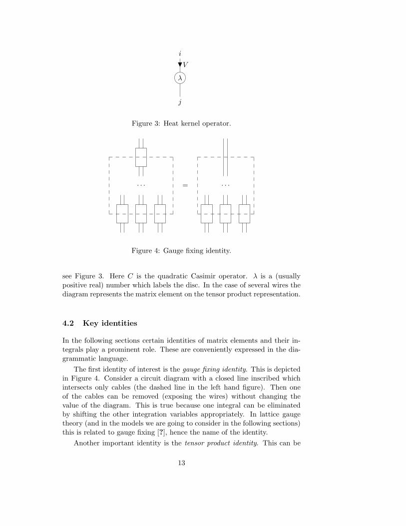
Figure 4: Gauge fixing identity.

see Figure 3. Here C is the quadratic Casimir operator. λ is a (usuallypositive real) number which labels the disc. In the case of several wires thediagram represents the matrix element on the tensor product representation.

4.2 Key identities

In the following sections certain identities of matrix elements and their in-tegrals play a prominent role. These are conveniently expressed in the dia-grammatic language.

The first identity of interest is the gauge fixing identity. This is depictedin Figure 4. Consider a circuit diagram with a closed line inscribed whichintersects only cables (the dashed line in the left hand figure). Then oneof the cables can be removed (exposing the wires) without changing thevalue of the diagram. This is true because one integral can be eliminatedby shifting the other integration variables appropriately. In lattice gaugetheory (and in the models we are going to consider in the following sections)this is related to gauge fixing [?], hence the name of the identity.

Another important identity is the tensor product identity. This can be

13

N H

N H

=I −1

N H

N H

Figure 5: Tensor product identity for irreducible representations. All wirescarry the same label.

Ω

=

Figure 6: Delta identity. The closed wire carries an Ω-label. Any numberof wires go through the cable.

expressed as ∫dg tVi,j(g)tVk,l(g

−1) =1

dimVδi,lδj,k,

where V is an irreducible representation. The diagrammatic form of theidentity is shown in Figure 5. Note also that for two inequivalent irreduciblerepresentations the result is zero.

Consider the identity defining the delta function, namely∫dg δ(g)f(g) = f(e).

Diagrammatically this is depicted in Figure 6. We refer to this for short asthe delta identity.

We also exhibit some useful identities involving the heat kernel oper-ator. The rather obvious fact that e−λCe−µC = e−(λ+µ)C translates intoFigure 7.a. Also important is the jump identity, Figure 7.b, where each wirecan stand for any number of wires. Furthermore, we can combine the jumpand the delta identity, see Figure 8.

What is remarkable is that all these identities (in their diagrammaticform) continue to hold in a rather general category theoretic context, in-cluding a quantum group setting [?, ?]. (The heat kernel operator is notmentioned there but one can take in general an appropriate natural trans-formation of the identity functor to obtain its properties.)

14

λ

µ= λ + µ

λ

=λ

(a) (b)

Figure 7: Identities involving the heat kernel factor: (a) addition, (b) jump.The labels on the wires are irrelevant.

λ

Ω

= λ

Figure 8: Modified delta identity with heat kernel factor inserted. It isobtained by combining the jump identity (Figure 7.b) and the usual deltaidentity (Figure 6).

15

5 Discrete gauge theory models

The background-free models we study in this paper are all (essentially) dis-crete quantum gauge theories. Prototypical and well suited to test ourapproach to renormalization are quantum BF theory and a generalization ofdiscrete quantum Yang-Mills theory (lattice gauge theory). Both are treatedin the present section.

Quantum BF theory is essentially topological and we show how thiscomes out in our approach. We then show how the anomaly that preventstrue topological invariance arises from a non-trivial action of the renormal-ization groupoid on a global parameter. From this the known change ofnormalization can be derived that leads to a topological theory, i.e. to arenormalization groupoid fixed point.

Discrete quantum Yang-Mills theory is more interesting from the point ofview of renormalization. Removing the background, the information aboutthe metric condenses into local parameters. One obtains a generalization oflattice gauge theory which might be called cellular gauge theory. It containsBF theory in its parameter space as a weak coupling limit. We discuss gen-eral features of the renormalization groupoid flow. While an open problem inhigher dimensions, an exact renormalization can be carried out in dimensiontwo. We show how this involves a non-trivial action of the renormalizationgroupoid on the local parameters.

We restrict ourselves in the following to considering no observables butpartition functions only. That is, renormalization is to be understood purelyas renormalization with respect to keeping the partition function fixed.

5.1 Quantum BF theory

5.1.1 Discretization and quantization

While really being interested in the discrete model (2) we start by brieflyrecalling its motivation as the quantization of continuum BF theory. Formore details on this subject we recommend [?].

Let M be a compact manifold of dimension n, G a compact Lie groupand P a principal G-bundle over M . We consider a connection A on P andan n − 2 form B with values in the vector bundle associated to P via theadjoint action. Define the action

S =∫

Mtr(B ∧ F ), (1)

where F is the curvature 2-form of A and tr is the trace in the fundamentalrepresentation.

We perform path integral quantization to obtain the partition function

Z =∫DADB eiS .

16

Formally integrating out the B-field leads to

Z =∫DAδ(F ),

i.e. we obtain the integral over all connections with vanishing curvature.To make sense of this expression we discretize M and proceed as in

lattice gauge theory, i.e. by assigning parallel transports to edges, curvatures(holonomies) to faces etc. However, not having any fixed background thereis no canonical or “regular” way of choosing a discretization. We needto consider arbitrary discretizations. That is, in the language introducedabove, cellular decomposition of M . Let C be such a cellular decompositionand K the 2-skeleton K of the dual complex (see the end of Section 2).As in lattice gauge theory we express the connection A through its paralleltransports along edges e of K. The curvature is then measured on each facef through the holonomy around the face, i.e. the product of the paralleltransports around the face. The measure over connections becomes theproduct of Haar measures per edge. That is, we obtain the discretizedpartition function

ZBF =∫ ∏

e

dge

∏f

δ(g1 · · · gk). (2)

Here δ is the delta function on the group and g1, . . . , gk are the group ele-ments associated with the edges that bound the face f . Note that in writingthis expression one chooses an orientation for each edge, an orientation foreach face and a starting vertex in the boundary of each face. However, allthese choices are irrelevant as the delta function is invariant under conjuga-tion and the Haar measure is invariant under inversion.

We proceed to express the partition function (2) in terms of circuit dia-grams [?, ?]: For each edge we obtain an unmarked cable representing theassociated group integral. For each face we obtain a wire going around theface through all the cables on the bounding edges. The wires represent thedelta functions and are marked Ω.

We can think of the obtained circuit diagram as embedded into themanifold. A piece of such an embedded diagram in three dimensions isshown in Figure 9. It is indeed this representation of the partition functionas a diagram embedded into the manifold which considerably simplifies thediscussion of renormalization.

Explicitly expanding the delta functions in the partition functions incharacters we obtain

ZBF =∑Vf

(∏f

dimVf)∫ ∏

e

dge

∏f

χVf(g1 · · · gk). (3)

17

Figure 9: Piece of embedded circuit diagram for quantum BF theory. Thepicture shows a three dimensional example. Labels and arrows on wires areomitted.

Here the sum runs over all assignments Vf of irreducible representations tofaces f . This corresponds diagrammatically to the expansion in Figure 2.One might consider this a more proper version of discrete BF theory than(2) as it contains explicit representation valued degrees of freedom whichcan be considered the discrete version of the B-field.

Reformulated in the spin foam formalism the partition function (3) yieldsin dimension three the Ponzano-Regge model [?] and in dimension four theOoguri model [?].

5.1.2 Exact renormalization

The proof of topological invariance of (anomaly corrected) quantum BFtheory in dimension three using the present formalism of circuit diagramsand certain cellular moves was already exhibited in [?]. We extend this hereto a full renormalization treatment and perform the (surprisingly simple)generalization to arbitrary dimensions.

The first step in understanding the renormalization of quantum BF the-ory is to investigate the change of the partition function ZBF under changeof cellular decomposition. Thanks to Conjecture 2.4 it is sufficient to regardthe change of ZBF under the cellular moves.

As ZBF is encoded in the embedded circuit diagram constructed abovewe need to compare the circuit diagrams before and after the application of

18

move initial configuration final configuration

n

n− 1

n− 2

Table 1: The effect of the cellular moves on the circuit diagrams. Therelevant cells as well as the embedded cables (boxes/cylinders) and wires(thicker lines) are shown.

19

the respective move. This is shown in Table 1. Only the parts of the circuitdiagrams affected by the moves are shown. Furthermore, only the moves oftype n, n − 1 and n − 2 are indicated. The other moves do not affect cellsof dimension ≥ n− 2 and thus leave the circuit diagram unchanged.

So, how does the value of ZBF change? Comparing Table 1 with Figures 4and 6 we find that both the n as well as the n−1 move leave ZBF invariant.This is due respectively to the gauge fixing and the delta identity. Bycontrast, the n− 2 move removes a factor corresponding to a closed Ω-loop,i.e. a factor of κ.1

Now we shall consider the renormalization of ZBF, i.e. we wish to con-struct an action of the cellular groupoid on parameters of the model suchthat ZBF becomes invariant. The model as defined by (2) has no parameters.We need to modify it by introducing parameters. However, as we have seenwe only have to compensate for factors of κ which carry no local informationof the model. It is sufficient to introduce a global integer parameter p whichcounts these factors. We define the partition function of the modified modelsimply as

ZBF := κpZBF. (4)

It remains to define the actions of the moves. We let the moves of typen, n−1, n−3, n−4, . . . act trivially while we let the move of type n−2 actby sending p 7→ p + 1 and its inverse by sending p 7→ p − 1. This preciselycancels the factor κ appearing in the circuit diagram for the n−2-move. Weobtain an exact renormalization.

The renormalized model has a free global parameter p. To specify it,one has to specify its value in a given cellular decomposition. This de-termines it, by the action of the renormalization groupoid, for all cellulardecompositions. From the point of view of the classical continuum modelthe discretization allows an exact quantization (i.e. not depending on it) upto the anomaly manifest in p.

Alternatively, we can fix the extra parameter p by making it explicitlydepend on the numbers ck of cells of given dimension k. For example wecan set2

p := −cn + cn−1 − cn−2.

It is easy to see that p defined in this way is changed only by moves of typen − 2, and exactly in the right way. Indeed we can make this part of thedefinition of the model instead of its renormalization. The action of the

1We shall not worry about the fact that this factor is divergent. Although we renor-malize here with respect to the partition function, what is finally relevant are physicalobservables which should be finite.

2Other choices are obtained for example by adding integer multiples of the Euler char-acteristic χ := cn − cn−1 + cn−2 − . . . of M .

20

renormalization groupoid is then trivial. The model is then independentof the cellular decomposition, it is a renormalization groupoid fixed point.3

When referring to quantum BF theory in the following we will usually meanthis version (4) where the anomaly has been fixed in some suitable way.

5.2 Generalized Yang-Mills theory

To talk about renormalization might seem somewhat artificial in the con-text of quantum BF theory. Indeed we saw that there is only one globalparameter involved which can be easily absorbed into a redefinition of thepartition function. As a less trivial example we discuss Yang Mills theoryin this section.

It might seem surprising that we apparently wish to consider a theorythat is defined on a metric background. However, we really consider ageneralization of Yang-Mills theory that naturally arises in a discretizedsetting [?]. This provides a nice example of how a background structure canbe turned into local parameters. These local parameters are then preciselywhat the renormalization groupoid acts on.

5.2.1 Discretization and quantization

We start again from a continuum formulation. Let M be a compact manifoldof dimension n, G a compact Lie group and P a principal G-bundle overM . Imagine we have some theory, determined through an action S whichdepends on a connection A on P . In order to define a quantum theory viaa path integral4

Z =∫DAe−S ,

we discretize the manifold M via a cellular decomposition C of M .We proceed as above, i.e. we discretize the connection by associating

parallel transports to edges e and holonomies to faces f of the 2-skeleton ofthe dual complex. The most general local5 gauge invariant action is thengiven by

S =∑

f

σf (g1 · · · gk),

3We suppose here as everywhere the validity of Conjecture 2.4. However, somethingweaker is sufficient for our reasoning to hold. Compare the respective remarks in Section 7.

4Note that we choose a Euclidean path integral. This is in accordance with standardpractice in lattice gauge theory. We are not interested in physical implications of suchchoices here.

5Local means here that interactions take place only within each face. In lattice gaugetheory terminology this is called “ultra-local”.

21

where g1, . . . , gk are the group elements associated to the edges that boundthe face f . σf is a choice of class function for each face f . This yields thepartition function

ZCGT =∫ ∏

e

dge

∏f

ρf (g1 · · · gk),

where we set ρf := e−σf .Indeed we see immediately that it is a generalization of the quantum BF

theory partition function (2). Decomposing ρf into characters

e−σf =∑V

αV,fχV ,

yields

ZCGT =∑Vf

(∏f

αVf ,f )∫ ∏

e

dge

∏f

χVf(g1 · · · gk). (5)

Here the sum over irreducible representations for each face is taken to thefront as a sum over assignments of an irreducible representation Vf to eachface f (compare (3)). As (5) is a generalization of lattice gauge theory tocellular decompositions we call it cellular gauge theory in the following.

From this expression we can read off the diagrammatic representation ofZCGT [?]. The circuit diagram is exactly the same embedded graph as for BFtheory (Figure 9). Only now the summation over irreducible representationsfor each closed wire (corresponding to each face) cannot be hidden in Ω labelsfor the wires. Instead the wires must carry explicit labels and the sum overdiagrams is performed with the weight factor (

∏f αVf ,f ).

Note that the partition function (5) has locally infinitely many parame-ters. For each face f there is a choice of parameter αV,f for each irreduciblerepresentation V (of which there are infinitely many). In the following werestrict ourselves to a more manageable situation. We set

αV,f := (dim V ) e−λf CV , (6)

where CV is the value of the quadratic Casimir operator on V and λf is apositive real parameter depending on the face.

We now turn to the relation with Yang-Mills theory. Assume that Mis equipped with a flat metric and that C is a cellular decomposition of Minto hypercubes of equal side length a. We set all λf equal to λ := an−4γ2.Then it can be shown that in the limit a→ 0 the action defined in this wayapproximates the continuum action of Yang-Mills theory (up to a constant)

SYM = − 1γ2

∫M

tr(F ∧ ?F ),

22

←−−−λ→0

λ −−−→λ→∞

Figure 10: The two limits of the heat kernel operator.

with coupling constant γ. Indeed, this is at the foundation of lattice gaugetheory (see e.g. [?]) and the discrete action we arrived at is nothing but theheat kernel action of lattice gauge theory. Note that that λ plays the roleof (the square of) a coupling constant.

Observe that the heat kernel operator e−λC has two interesting limits,λ → 0 and λ → ∞. In the first case it just becomes the identity. In viewof the above this implies that quantum BF theory can be considered theweak coupling limit (λ = 0) of lattice gauge theory, since we then recover(3) from (5). The opposite regime (λ → ∞) is that of strong coupling oflattice gauge theory. The low dimensional representations dominate moreand more in the partition function. At the extreme point λ = ∞, onlythe trivial representation contributes, onto which the heat kernel operatorbecomes a projector. Diagrammatically the limits can be expressed as inFigure 10.

Let us go back to the case of interest, that of a topological manifold Mwith arbitrary cellular decomposition C. Note that the above relation alsosuggests to view λf as a remnant of a local metric. As we shall see belowthis statement can be made precise in the case of dimension two.

Diagrammatically, the choice (6) means that we can put the heat ker-nel factor per face f into the circuit diagram as a disc with label λf . Thesummation over irreducible representations with the remaining factor of di-mension can then be indicated by Ω-labels for all the wires.

5.2.2 Renormalization in general

We start by investigating the change in ZCGT under the moves. Using thediagrammatic representation this step is almost identical to what we did forquantum BF theory. Indeed, again the relevant parts of the diagrams areas shown in Table 1. The difference is that we now sum over irreduciblerepresentations for each wire with a weight that is not the dimension, as canbe indicated by an extra disc diagram per wire.

This makes no difference for the n-move, as the gauge fixing identity(Figure 4) does not depend on attached labels. For the n−1-move, however,the delta identity (Figure 6) that ensured invariance in the BF case can nolonger be applied. The weight in the summation over representations for the

23

closed wire is no longer the dimension. For the n − 2-move there is againjust a mismatch of a factor, which is now

κf :=∑V

(dim V )αVf ,f =∑V

(dim V )2e−λf CV .

In summary, the most crucial difference to quantum BF theory is the break-ing of invariance under the n− 1-move.

Let us turn to the problem of renormalization. As before, the treatmentof the n− 2-move is relatively easy. Redefining the partition function to be

ZCGT := (∏f

κ−1f )ZCGT,

fixes the n−2-move, i.e. makes ZCGT invariant under it. On the other hand,this makes the non-invariance under the n− 1-move worse in the sense thatit would now be broken even in the limit λf = 0. To remedy this and obtainthe renormalization groupoid fixed point of quantum BF theory in this limitone could include a factor of κ−cn+cn−1 (compare Section 5.1.2).

The renormalization of the n − 1-move poses much deeper problems.Superficially it seems that instead of applying the delta identity, we haveto apply the modified delta identity (Figure 8). Indeed we can do this andperhaps this is really a first step towards tackling the general problem. How-ever, the circuit diagram we arrive at is not of the same kind as the originalcircuit diagram: The shifted heat kernel diagram extends over several wires.

Although no general solution to the problem is known, qualitative fea-tures of the renormalization groupoid flow are easily described. Firstly, theparameter space of cellular gauge theory contains two fixed points (we as-sume the anomaly has been fixed as described above). The first one, at λ = 0(weak coupling limit) is quantum BF theory while the second one at λ =∞(strong coupling limit) is a trivial theory. (In the latter all representationsare trivial and invariance under the moves is trivially satisfied.)

Secondly, we can say something about the direction of the renormaliza-tion groupoid flow. Consider a region of the manifold with some given pa-rameter values λf . Roughly speaking, we can perform a refinement withoutchanging the partition function by assigning to the newly created parametersthe topological value λf = 0. Now the partition function in the refined re-gion should be left unchanged if we average the parameters λf in this regionin some suitable way. That is, the average value of the parameters (of whichthere are now more) has decreased compared to the unrefined situation. Insummary, if we coarsen, the parameters λf must generally increase to keepthe partition function fixed. The renormalization groupoid flow goes in thedirection from lower values of λf in the ultraviolet to higher values in theinfrared.

This general behaviour applies in particular close to the renormalizationgroupoid fixed points. (Consider for example a situation where only a few

24

∗ ∗FP FP

λ = 0 λ =∞UV IR

Figure 11: Qualitative picture of the renormalization groupoid flow for cel-lular gauge theory (generalized discrete quantum Yang-Mills theory). Thetwo fixed-points are quantum BF theory in the weak coupling limit (λ = 0)and the trivial theory in the strong coupling limit (λ = ∞). The generaldirection of the flow is from the first (UV) fixed-point to the second (IR).

λf are non-zero or non-infinite.) Thus, quantum BF theory is a (repulsive)UV fixed point while the trivial theory is an (attractive) IR fixed point.6

This is schematically illustrated in Figure 11.

5.3 Exact renormalization in dimension two

In the case of dimension two an exact renormalization can be performedwhich confirms the qualitative picture. As lattice gauge theory is solvablethen [?] this is not at all surprising. That things can be made well in thiscase is rather obvious in our approach. As each cable has only two wires(because each edge bounds only two faces), the shifted heat kernel factoragain sits on a single wire.

As there is no n − 2-move in dimension n = 2 we consider the originalpartition function ZCGT (and not ZCGT). Now, after applying the modifieddelta identity, we can combine the shifted heat kernel factor with the onethat was attached to the wire before via addition (Figure 7.a). We simplyget the heat kernel factor for the sum of the parameters.

The solution of the renormalization problem in dimension two is thusas follows. The 2-move acts trivially. The 1-move acts by sending the pairof parameters (λf1 , λf2) to λ′f2

= λf1 + λf2 . Here, f1 denotes the 0-cell (orface) that is removed, f2 denotes the other 0-cell (or face) with which f1 wasconnected through a 1-cell (edge). The new parameter value λ′f2

replacesthe old one for f2. The so defined action leaves ZCGT invariant and is localin the sense of Definition 3.2.

6Note a subtle difference to the conventional situation with continuous scale trans-formations. There, one would get arbitrarily close to the IR fixed point by further andfurther coarsening (increasing the scale). In our case the manifold is compact and thereare maximally coarse decompositions. Consequently, for any given starting point (whichis not the IR fixed point) the renormalization groupoid flow stops at a finite distance fromthe IR fixed point.

25

Note that the action is not defined for the whole cellular groupoid, butonly in the direction of coarsening. (An action of the inverse 1-move is notdefined.) This is due to the impossibility of unambiguously recreating localparameters and goes hand in hand with the idea of integrating out degreesof freedom (see the discussion at the end of Section 3.2).

Coming back to the interpretation of cellular gauge theory as Yang-Millstheory we can give the local parameters indeed a simple meaning in terms ofmetric information. We can think of λf as (proportional to) the area of theface f . The 1-move might then be thought of as the merging of two faces,thus giving the new face the sum of the areas.

It is sometimes said that 2-dimensional Yang-Mills theory is topological.This is not true in our terminology, i.e. it is not a renormalization groupoidfixed point. However, its renormalization is exact and rather simple. Ofcourse, it is even simpler in the context of lattice gauge theory where alllocal parameters are identical and thus only one parameter changes underchange of scale.

As a side remark, we observe that it is very easy to solve the two dimen-sional theory using the diagrammatics [?]. Just apply the tensor productidentity (Figure 5) to all cables. Only closed loops of wire without any ca-bles are left. Counting the loops and taking care of the heat kernel factorsone obtains immediately

ZCGT =∑V

(dim V )χ e−CV∑

f λf ,

where χ = c2 − c1 + c0 is the Euler characteristic of M and the sum runs asusual over the irreducible representations of G. This agrees of course withthe well known solution of lattice gauge theory [?]. Moreover, the diagram-matic solution carries over directly to the quantum group case, yielding thesame expression [?]. (Then “dim” denotes the quantum dimension and CV

some suitable quantum Casimir operator.)

6 Spin foam models of quantum gravity

In this section we consider certain spin foam models of Euclidean quan-tum gravity in the light of our approach to renormalization. These arethe Reisenberger model [?], the Barrett-Crane model [?], and a new modelinterpolating between the latter and quantum BF theory.

For all considered models the problem of renormalization is nontrivial asthey depend on the discretization of space-time in a nontrivial way. Findinga solution to the renormalization problem being far beyond the scope ofthis paper we limit ourselves to a first step. That is, we investigate thequestion of amenability of these models to a renormalization treatment.This implies identifying suitable local degrees of freedom that can be acted

26

upon by the renormalization groupoid. Since these degrees of freedom arepresent neither in the Reisenberger model nor in the Barrett-Crane modelwe propose modifications of both models that carry such degrees of freedom.

6.1 Motivation: BF theory plus constraint

For the reader’s convenience we review very briefly the motivation of thepresent models as quantizations of general relativity (see [?] for more de-tails).

Let M be a compact four dimensional manifold (space-time) with aSpin(4) principal bundle. Consider a 1-form e (the vierbein) with valuesin the Lie algebra of Spin(4) and a spin connection A. Let F be the curva-ture 2-form of A and consider the action

S =∫

Mtr(e ∧ e ∧ F ).

This describes Euclidean general relativity (assuming e to be non-degenerate).While this is difficult to quantize one can observe a certain similarity

with BF theory (1). Indeed we can take the BF action if we introduce theadditional constraint that the B-field arises from an e-field, i.e.

B = e ∧ e. (7)

The idea is now to quantize BF theory, which we know how to do (seeSection 5.1) and impose the constraint (7) afterwards. The latter step israther nontrivial and various proposals for its implementation have beenmade. Perhaps the best known ones are the model due to Reisenbergerand the one due to Barrett and Crane. These are the ones we are going todiscuss.

6.2 The Reisenberger model

Since the spin group in four dimensions is Spin(4) = SU(2)× SU(2) we candecompose the spin bundle into two “chiral” components, one for each copyof SU(2). One can then observe that one chiral component is enough toformulate classical general relativity. This carries over to the above contextof obtaining general relativity by constraining BF theory.

The Reisenberger model [?] thus starts with quantum BF theory (2)with gauge group SU(2). It is formulated on a simplicial decomposition ofspace-time. The partition function is given by

ZRei =∫ ∏

e

dge

∏v

(z√

2π)−5[e−1

2z2 ΩijΩij

]∏f

δ(g1 · · · gk). (8)

27

∗ ×FP

λ = 0 λ =∞

Figure 12: Qualitative picture of the renormalization groupoid flow for boththe Reisenberger and the interpolating model. There is one ultraviolet fixed-point at λ = 0 which is quantum BF theory. There is another special pointat λ = ∞ (or z = 0) which for the interpolating model corresponds to theBarrett-Crane model.

What is different as compared to quantum BF theory is the factor

(z√

2π)−5[e−1

2z2 ΩijΩij

] (9)

inserted for each vertex. z is a real parameter of the model while Ωij denotesa certain operator. Ωij is a sum of operators each of which acts on a pair ofdelta functions associated with the given vertex. Diagrammatically speakingit acts on all pairs of wires (belonging to pairs of faces or 2-simplices) whichare associated with the vertex (i.e. which belong to the 4-simplex). We willnot give the full definition here as this is irrelevant for our considerations.

The model as defined is not immediately amenable to a treatment in ourapproach. A serious problem is the fact that it is only defined for simpli-cial decompositions. Thus, although the cellular moves can be applied inprinciple the resulting configurations are not simplicial and thus not com-parable to the original model. An interesting alternative would be to try todefine the model for cellular decompositions through the moves. Howeverthis would presumably involve solving the renormalization problem and isthus beyond the scope of our current investigation.

Another prerequisite to a renormalization in our sense are tunable localparameters. These are easily introduced into the partition function. Onecan simply let the real parameter z depend on the vertex, i.e. introduceone zv per vertex. What is more, for zv → ∞ we (essentially, i.e. up tonormalization) recover quantum BF theory. That is, our parameter spacecontains a renormalization groupoid fixed point (up to an anomaly whichcan be easily eliminated, see Section 5.1).

Assuming the difficulties can be overcome we can nevertheless make some

28

qualitative remark on the the renormalization groupoid flow. For bettercomparability with the other models we consider inverted parameters λ ∼=z−1. We also disregard the first factor in (9) which should not be relevantfor the qualitative picture. The model is rather similar to cellular gaugetheory in the vicinity of the quantum BF theory fixed point. Indeed, in thisregion the arguments concerning the flow put forward in Section 5.2.2 apply.That is, the flow points away from the “weak coupling limit” λ = 0 which isa repulsive ultraviolet fixed-point. On the other hand, the point λ = ∞ isnot a fixed point and it is not clear how the flow behaves near it. Figure 12shows a diagrammatic illustration of the situation.

6.3 The Barrett-Crane model

While different versions of the Euclidean Barrett-Crane model have beenproposed [?, ?, ?, ?, ?] we consider a version which appears to be the mostnatural one in our framework. For ease of terminology we refer to it in thefollowing as “the” Barrett-Crane model.

While originally defined for simplicial complexes only it was shown byReisenberger that the Barrett-Crane model naturally extends to more gen-eral complexes [?]. Our treatment in the following directly applies to generalcellular decompositions. It is closely related to the connection formulationof which an extensive treatment can be found in [?].

We start with the full Spin(4) BF theory in four dimensions. To describethe crucial step of implementing the constraint (7) it will be convenient toexplicitly perform the decomposition into chiral components. Writing eachgroup element and matrix element as a product of left-handed and right-handed chiral SU(2) component the partition function (2) decomposes intothe product of two BF partition functions

ZBF =∫ ∏

e

dgLe dgR

e

∏f

δ(gL1 · · · gL

k )δ(gR1 · · · gR

k ). (10)

Here the superscripts L and R denote the chiral components.This step finds its diagrammatic expression in the splitting of the circuit

diagram for the partition function (Figure 9) into two identical diagramsfor SU(2), one for each chiral component. Note that the representationlabels for the diagrams are now SU(2) representation labels, summed overindependently.

We stick in the following to a purely diagrammatic representation ofthe partition function. This avoids on the one hand writing complicatedformulas and on the other hand facilitates understanding the structure ofthe model in view of the renormalization problem. It also avoids extracomplications arising for non-simplicial decompositions in the spin foamformulation.

29

L

L R

R

Figure 13: In going from BF theory to the Barrett-Crane model one insertsthe cables between the dotted lines. There is one such cable for each chiralpair of wires. Here is shown an edge with four wires, the only case occurringin a simplicial decomposition in dimension four. Labels and arrows on wiresare omitted.

As a second step we replace each cable by a sequence of two cables. Thisis a special case of the (inverse) gauge fixing identity (Figure 4) and thusdoes not change the partition function. It implies algebraically another (re-dundant) doubling of the group variables, so that for each chiral componentthere is now one group variable attached to each end of each edge.

So far we have only rewritten the partition function without changingit. The Barrett-Crane model is now obtained by inserting further cables oneach edge between the cables present. This is depicted in Figure 13. Onecable is inserted for each chiral pair of wires, so that the pair of wires goesthrough the cable. This has the effect of projecting onto “simple” irreduciblerepresentations of Spin(4), i.e. those where both chiral components are thesame representation of SU(2). It is designed to implement the constraint(7). The partition function ZBC of the Barrett-Crane model is defined bythis circuit diagram. The conversion of the diagram into a closed formula isagain straightforward, by inserting a group integral for each cable etc.

Although the circuit diagram appears to be quite complicated at thispoint it can be simplified considerably. As the Barrett-Crane cables justcarry two wires with irreducible representations we can apply the tensorproduct identity (Figure 5). This forces the two chiral components to liein the same representation and and leads to a decomposition of the circuitdiagram. Indeed we obtain a separate circuit diagram for each vertex (or n-

30

Figure 14: The circuit diagram for a 4-simplex in the Barrett-Crane model.Labels and arrows on wires are omitted.

cell). After repeated application of the gauge fixing identity (Figure 4) thisconsists of one cable per edge (n− 1-cell) and one wire per face (n− 2-cell)that meet the vertex (n-cell). An easy way to construct this diagram is asfollows: Consider the part of the circuit diagram for BF theory that lies inan n-cell. Cut it out (this cuts cables in halves) and produce a mirror image.Now connect the diagram and its mirror image in the obvious way to obtaina closed diagram. The two parts correspond exactly to what were before thetwo chiral components. For a 4-cell which is a simplex the diagram obtainedin this way is drawn in Figure 14.

The whole partition function can be reexpressed as

ZBC =∑Vf

(∏f

(dim Vf )2−|∂f |)∏v

Av(Vf ). (11)

Here the summation is over labelings Vf of faces with irreducible representa-tions of SU(2), |∂f | denotes the number of edges of face f and Av(Vf ) is thevalue of the circuit diagram for the vertex v (with the appropriate labels).The origin of the exponent |∂f | lies in the fact that each application of thetensor product identity (Figure 5) produces a factor of inverse dimension.7

Other versions of the Barrett-Crane model agree with the present one inthe vertex amplitude Av(Vf ), while differing in the choice of weights for edges

7Note that there is a subtlety associated with certain cellular decompositions whichdoes not arise for simplicial ones. Namely, there can be 2-cells which are not in theboundary of any 3-cell. In the dual language, these are faces which have no edge. In thiscase the associated wires (which are just loops) would not carry any projecting Barrett-Crane cable. That is, for those particular wires one still has to sum over chiral SU(2)representations separately. This would give a modification to (11). On the other hand onecould by definition restrict the chiral components to be equal also for those wires so as toarrive at (11).

31

and faces. For example, the Perez-Rovelli version [?] is obtained if insteadof inserting one layer of Barrett-Crane cables as in Figure 13 two such layersare inserted with another “LR layer” inbetween. We explain below why thepresent choice stands out in view of a renormalization treatment.

As a first step in investigating renormalization properties of the Barrett-Crane model we apply the moves to the model “as is”. One quickly sees thatneither the n- nor the n− 1-move preserve the partition function in any ob-vious way. Indeed, for the n-move one removes a subdivision between n-cells(i.e. merges two vertices) so that before the move one has two disconnecteddiagrams while afterwards there is one connected diagram. Except for triv-ial cases there seems to be no way how they could be equal. This is not asurprise. The relevant identity for quantum BF theory was the gauge fixingidentity. It reflects the possibility of fixing a gauge and is based on gaugeinvariance (see [?]). However, the Spin(4) gauge invariance is precisely bro-ken in the Barrett-Crane model (to a SU(2) subgroup) by the introductionof the extra cables which act as projectors.

For the n−2-move the situation is similar to quantum BF theory. Beforethe move one has factors of dimension which are not present after the move.See footnote 7 however.

6.4 An interpolating model

As the Barrett-Crane model is not invariant under the cellular moves, i.e. nottopological, a renormalization treatment in our sense would require local pa-rameters. On top of that one would like to have a renormalization groupoidfixed point in the ultraviolet analogous to the weak coupling regime in cel-lular gauge theory (Section 5.2) and the large z regime in the Reisenbergermodel (Section 6.2).

Based on these requirements we propose a new model as follows: TheBarrett-Crane model is defined as a modification of quantum BF theory(which is topological). It is thus natural to tune the way this modificationis performed. More precisely, as above, we start with BF theory of Spin(4),rewriting it in terms of the chiral decomposition and the extra doubling ofthe cables for each edge. Then, instead of proceeding to insert cables as inFigure 13 we insert heat kernel factors as appearing in lattice gauge theory(see Section 5.2). Instead of arriving at the diagram of Figure 13 we arriveat the diagram of Figure 15 per edge. This defines the partition functionZInt of the model.

The present definition uses the two limits of the heat kernel operatore−λC (Figure 10). For λ → 0 we recover quantum BF theory while forλ → ∞ we get the usual Barrett-Crane model. The local parameters wehave introduced are one positive real number per edge and face. If desiredone could decrease the number of parameters by requiring them to be thesame within a face or within an edge.

32

L

L R

R

λ1 λ λ λ2 3 4

Figure 15: Edge diagrams for the interpolating model. λi are positive realparameters. There is one such parameter per edge and face. Labels andarrows on wires are omitted.

Considering qualitative aspects of the renormalization groupoid flow wehave now the same scenario as for the Reisenberger model (Figure 12). At“weak coupling” (small λ) the arguments of Section 5.2.2 again apply. Therenormalization groupoid flow is directed away from the ultraviolet fixedpoint given by quantum BF theory at λ = 0. On the other hand, much lessis known about the point λ = ∞ which corresponds to the Barrett-Cranemodel.

However, a numerical study of different versions of the Barrett-Cranemodel was conducted by Baez et al. [?]. This includes in particular the Perez-Rovelli version [?]. It turns out that the partition function in this case isstrongly dominated by contributions with almost all representations trivial.It should be expected that our version of the Barrett-Crane model behavessomewhat similar, although not quite as extreme. This would suggest thatat the point λ = ∞ of the interpolating model (where the Barrett-Cranemodel resides) we have “almost” a trivial theory, to be compared with theIR fixed point in cellular gauge theory.

In retrospect we have now an additional argument for our choice ofweights for edges and faces for the Barrett-Crane model (manifest in (11)).We see now that it is not only natural in the way the model is constructedfrom quantum BF theory but essential in obtaining an ultraviolet fixed pointin the parameter space of the interpolating model.

33

7 Discussion and conclusions

A crucial issue that we have not addressed in the present paper is the roleof observables. Indeed, for a sensible physical interpretation what we needis not a renormalization that keeps the partition function fixed but onethat preserves physical observables. Nevertheless, the two might be closelyrelated. Indeed, for quantum BF theory the two notions coincide if we takeobservables to be Wilson loops. This is why (quantum group versions) of thismodel give rise both to invariants of manifolds and knots (the knots beingWilson loops), see [?]. The same is true for cellular gauge theory (quantumYang-Mills theory) in dimension two. If we keep the “area” (the sum of thelocal parameters) inside a Wilson loop fixed, the expectation value of thelatter is exactly preserved by the renormalization that we presented.

The situation is rather different for the models of quantum gravity thatwe have considered. Here, even the question of what the correct physicalobservables are is unresolved. Indeed, our qualitative statements concerningthe renormalization groupoid flow could be (and probably will be) sub-stantially altered if renormalization is performed with respect to relevantobservables. A further point is that while we have considered these modelsfor given topology and cellular decomposition it has been proposed to sumthem over discretizations (usually simplicial ones) of space-time and evenover topologies. However, to get control of such a sum it is presumably stillnecessary to understand and relate the individual terms (discretizations)and perform a renormalization in our sense.

One proposal for performing such a sum is that of a generating field the-ory [?, ?, ?, ?]. This is usually a field theory on the gauge group which gen-erates discretized space-times as its Feynman diagrams. This is particularlyeasy to see when using our diagrammatic language. Expressing propagatorsand vertices in terms of the diagrams of Section 4, a closed Feynman diagrambecomes exactly the circuit diagram representing the partition function ofthe respective model for the corresponding discretization.8

In general, a renormalization with respect to observables is a weakerproblem than a local renormalization with respect to the partition function.Namely, the latter implies the former but not the other way round. Forexample, in the quantum BF theory case, the anomaly cancels in expectationvalues. A related issue is that asking for an exact renormalization is often toomuch. A coarse discretization is not supposed to reproduce all the physicsof a finer one. Thus, one usually requires a renormalization to preserveobservables only in some approximate sense, for example have them convergein an “infinite refinement limit” as in lattice gauge theory.

While we have limited ourselves here to closed manifolds our frame-8Strictly speaking, one has to view Feynman diagrams as intertwiners in the represen-

tation category of the group. This is explained (among other things) in [?, ?]. Then oneuses the circuit diagrams to represent these intertwiners [?].

34

work extends straightforwardly to manifolds with boundary. Indeed, ourdefinitions in Sections 2 and 3 carry over practically unchanged. In addi-tion, gluing along boundaries is essentially straightforward for the models weconsider. For quantum BF theory and cellular gauge theory this is alreadyexplained in [?]. In a setting with boundaries renormalization groupoid fixedpoints correspond to topological quantum field theories (at least if an exactrenormalization of the partition function is required).

One could also envisage a special treatment of boundaries where theycarry extra parameters. This might be desirable if a fixed background isattached to a boundary. Such a situation could occur for example if inquantum gravity one wishes to put quasi-classical or coherent states on theboundary.

As we have emphasized it is rather important for renormalization inour sense to work to allow for cellular decompositions and not restrict tosimplicial ones. This is a problem in the Reisenberger model (considered inSection 6.2) whose definition strongly uses the fact that cells are simplices.A generalization of the model in this direction is thus desirable. In contrast,the formulation of the Barrett-Crane model (considered in Section 6.3) interms of cellular decompositions is straightforward. In this case however,local parameters allowing for a renormalization groupoid flow are absent.This prompted us to define an interpolating model that contains both theBarrett-Crane model and quantum BF theory in its (local) parameter space.To define this we “imported” the idea of heat kernel factors from latticegauge theory. This allows a continuous switching between a “weak couplinglimit” of quantum BF theory and the “strong coupling limit” of the Barrett-Crane model.

We suggested that the renormalization groupoid flow both in the Reisen-berger and in the interpolating model should behave similarly as for cellulargauge theory in the region of “weak coupling” (small λ). All these modelsshare the same renormalization groupoid fixed point of quantum BF theoryin the ultraviolet. On the other hand, while having a special point in the“strong coupling limit” of λ =∞ this is an infrared fixed point only for cel-lular gauge theory. Nevertheless, both for the Reisenberger model and forthe interpolating model one should expect behaviour somewhat similar tocellular gauge theory also in this region. In both cases, there are projectionoperators which are “maximally turned on” at λ = ∞ comparable to theheat kernel operators in cellular gauge theory. In contrast to the latter theydo not lead to a complete restriction to trivial representations. Nevertheless,they should have an effect approaching this.

For the Barrett-Crane model numerical investigations by Baez et al.seem to indicate indeed that the partition function is strongly dominatedby terms where almost all representations are trivial [?]. Baez et al. suggestthat such a situation might indicate a bad choice of weights for edges andfaces. Our conclusion is rather different. We propose that the Barrett-Crane

35

model should be considered as just a point in the parameter space of a moregeneral model (the interpolating model) which is rather more amenable toa renormalization. From this point of view it is even a welcome feature ifthe Barrett-Crane partition function is strongly dominated by terms withalmost all representations trivial. This would give the interpolating modelat “strong coupling” a region in parameter space which “almost” containsan infrared fixed point of the renormalization groupoid.

Markopoulou has made the interesting proposal [?, ?] to apply the renor-malization methods of perturbative quantum field theory to spin foam mod-els. Based on the structural similarity of spin foams with Feynman diagrams(which becomes a strict correspondence in the generating field theory ap-proach mentioned above) she suggests a Bogoliubov type recursion equationfor spin foams (formulated in a Hopf algebraic language). Her concept ofcoarsening is strictly based on spin foams but essentially coincides with theone coming from cellular decompositions in this context. Thus, one mighthope that her approach can fruitfully complement the one presented here.In particular, Markopoulou’s approach might be useful in eliminating cer-tain infinities (as the corresponding techniques in perturbative quantum fieldtheory do). Such infinities arise for example from summing over infinitelymany irreducible representations, as in quantum BF theory, compare (3).

The basic ideas on renormalization introduced in Sections 2 and 3 arenot specific to the gauge type models that we have considered in the latersections. Indeed they should be applicable to a wide range of models (includ-ing spin systems for example). Furthermore, while we have emphasized therole of background independence, this is not a requirement. Indeed, the pro-posed methods might be applicable to situations where a metric backgroundis present, but the discretization of space-time is nevertheless irregular (as in“random geometry” models). In such a situation metric information mightbe converted into local parameters. Indeed, we saw that this was a possiblepoint of view in our cellular gauge theory example of Section 5.2.

Much of our treatment seems to depend on Conjecture 2.4 and indeed itwould be important to establish its validity (or non-validity). However, thesituation is rather less serious. Firstly, even if the conjecture was false in itspresent form, it is very likely to hold under some mild technical assumptionsabout the manifold or cellular decomposition (such as piecewise linearity).Such assumptions very likely would have little or no physical relevance.Secondly, for the application to a given model it is usually not necessarythat the conjecture holds in all its aspects. For example, for all the modelsconsidered in this paper only the cells of dimension n, n − 1, and n − 2are relevant. Thus, a much weaker form of the conjecture suffices. Thirdly,considering a certain subclass of refinements or coarsenings might be enoughfor a sensible renormalization in a given context. Again, this would requireonly a weaker form of the conjecture.

While we worked throughout with a topological manifold it should be

36

possible to do away even with this “background”. A suitable setting in thepresent context would probably be that of (finite) CW-complexes. Conjec-ture 2.4 is definitely false if “n-dimensional manifold” is replaced by “n-dimensional CW-complex”. This is not surprising as the complex can con-tain “pieces” of lower dimension. On the other hand one could consider allcellular moves for all dimensions up to n (the dimension of the cell of maxi-mal dimension). This would give n(n+1)/2 moves. The analogue of Conjec-ture 2.4 would then state something like that any two finite decompositionsas CW-complexes (if they exist) of the same topological space are related bya sequence of these moves. The basic considerations of Section 3 concern-ing renormalization could then be carried over practically unchanged. Onecould be even more general by considering combinatorial complexes. How-ever, a quantum group generalization of models as considered here would bedefinitely lost in this case as it depends on certain topological information[?].

Acknowledgements

I would like to thank Hendryk Pfeiffer and Carlo Rovelli for valuable com-ments on the manuscript. Furthermore, I would like to thank Thomas Kra-jewski and Valentin Zagrebnov for discussions. This research was supportedby the European Union through a Marie Curie Fellowship grant.

37